End-to-End Driving via Self-Supervised Imitation Learning Using Camera and LiDAR Data

Abstract

In autonomous driving, the end-to-end (E2E) driving approach that predicts vehicle control signals directly from sensor data is rapidly gaining attention. To learn a safe E2E driving system, one needs an extensive amount of driving data and human intervention. Vehicle control data is constructed by many hours of human driving, and it is challenging to construct large vehicle control datasets. Often, publicly available driving datasets are collected with limited driving scenes, and collecting vehicle control data is only available by vehicle manufacturers. To address these challenges, this paper proposes the first self-supervised learning framework, self-supervised imitation learning (SSIL), that can learn E2E driving networks without using driving command data. To construct pseudo steering angle data, proposed SSIL predicts a pseudo target from the vehicle’s poses at the current and previous time points that are estimated with light detection and ranging sensors. Our numerical experiments demonstrate that the proposed SSIL framework achieves comparable E2E driving accuracy with the supervised learning counterpart. In addition, our qualitative analyses using a conventional visual explanation tool show that trained NNs by proposed SSIL and the supervision counterpart attend similar objects in making predictions.

Jin Bok Park Jinkyu Lee Muhyun Back Hyunmin Han David T. Ma Sang Min Won* Sung Soo Hwang* Il Yong Chun*

J. B. Park
Department of Electrical and Computer Engineering, Sungkyunkwan University, Suwon, Gyeonggi-do 16419, South Korea
Email address: bjb663@g.skku.edu

J. Lee
Department of Information and Communication Engineering, Handong Global University, Pohang, Gyeongsangbuk-do 37554, South Korea
Email address: jinkyu.lee@stradvision.com

M. Back
Department of Information and Communication Engineering, Handong Global University, Pohang, Gyeongsangbuk-do 37554, South Korea

H. Han
Department of Information and Communication Engineering, Handong Global University, Pohang, Gyeongsangbuk-do 37554, South Korea

D. T. Ma
College of Engineering, Texas A & M University – Corpus Christi, Corpus Christi, TX 78412, USA

S. M. Won
Department of Electrical and Computer Engineering, Sungkyunkwan University, Suwon, Gyeonggi-do 16419, South Korea
Email address: sangminwon@skku.edu

S. S. Hwang
School of Computer Science and Electrical Engineering, Handong Global University, Pohang, Gyeongsangbuk-do 37554, South Korea
Email address: sshwang@handong.edu

I. Y. Chun
School of Electronic & Electrical Engineering, and Departments of Artificial Intelligence, Electrical & Computer Engineering, Semiconductor Convergence Engineering, and Display Convergence Engineering, Sungkyunkwan University, Suwon, Gyeonggi-do 16419, South Korea
Center for Neuroscience Imaging Research, Institute for Basic Science, Suwon, Gyeonggi-do 16419, South Korea
Email address: iychun@skku.edu

1 Introduction

End-to-end (E2E) driving predicts driving commands (at one end) from sensory input (at the other end), and it is gaining rapid attention for autonomous driving vehicles.¹ The conventional modular approach accomplishes complex tasks of autonomous driving by using self-contained, but interconnected modules such as object detection, object tracking, localization, path planning and control.^{1; 2; 3} In the conventional modular approach in general, if a malfunction or unpredicted behavior is observed, one can diagnose a specific malfunctioning module, understanding decision-making processes behind the module.^{1; 2}

However, the conventional modular approach needs tremendous efforts to build, maintain, and optimize their modules, and is yet to achieve complete autonomy.^{1; 2; 4} In addition, input(s) and output(s) for each module might not be optimal for the ultimate driving task in various driving scenarios.

Different from the modular approach, the E2E approach, also known as behavior cloning, considers the entire processing and prediction pipeline as a single learnable machine-learning task.^{5; 6} The approach directly transforms sensory inputs to driving commands, such as steering angle, acceleration, and braking.⁷ However, with no intermediate outputs, it is much more difficult to trace the initial cause of a driving error as well as to explain why the E2E driving model arrived at specific driving decisions.¹ Some promising works for complete autonomy have been recently reported.³

Broadly speaking, an E2E driving model can be trained with the two approaches, imitation learning^{5; 6; 8; 9} and reinforcement learning^{10; 11; 7} The former approach learns E2E driving models to mimic human driver behavior¹². An E2E driving neural network (NN) is optimized to produce the same driving actions as humans, directly from its input data collected with camera(s), light detection and ranging (LiDAR) sensor(s), and/or inertial measurement unit(s). The latter approach learns E2E driving models to act optimally at each instant. The reinforcement learning for the E2E driving model trains which vehicle actions result in the best outcomes while navigating the driving environment.

For accurate and reliable autonomous driving, both approaches require human driving commands. Conventionally, imitation learning is supervised learning that requires (labeled) reference data, e.g., steering wheel angle control by human drivers.⁹ Reinforcement learning is in general known to be unsupervised learning but still requires a significant amount of training data generally with simulators.^{10; 11} Even though reinforcement learning itself only requires human intervention to reward the network, such human intervention is costly and several works pointed out that rewarding from the driving data of vehicles is necessary.¹¹ There exist several publicly available datasets for learning autonomous driving systems that provide data collected from sensors mounted on the exterior of vehicles. On the contrary, steering angle data is not always available. Furthermore, one can only access internal driving data such as steering angle with the assistance of vehicle manufacturers. To resolve the aforementioned challenges, one may estimate steering angles from sensory data, e.g., camera and LiDAR data.^{13; 14}

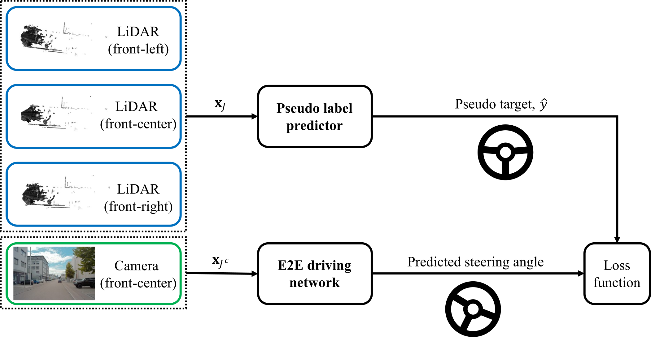
This paper proposes the first self-supervised learning framework for E2E driving, referred to as self-supervised imitation learning (SSIL). We modify the existing self-supervised regression learning approach,¹⁵ using domain knowledge in LiDAR sensors, vehicle geometry, steering geometry,¹⁶ etc. To construct pseudo steering angle data, we estimate the vehicle pose for each time frame from point clouds obtained by three LiDAR sensors, and predict a pseudo-label at each time point, using the estimated poses from two consecutive time frames and domain knowledge regarding the vehicle. Figure 1 overviews the proposed SSIL framework to learn an E2E driving NN without using expert driving commands. Our numerical experiments show that the proposed SSIL framework achieves comparable E2E driving accuracy with the supervised learning counterpart. To better understand how a NN trained by proposed SSIL predicts driving commands, we compare their saliency maps with those of a trained NN by ordinary SIL, with the conventional visual explanation tool VisualBackProp.¹⁷

The paper is organized as follows:

• Section 2 develops some backgrounds of existing self-supervised regression learning.¹⁵

• Section 3 proposes the SSIL framework. In particular, we design a pseudo-label predictor as the composition of two functions, based on some domain knowledge about sensors and the vehicle. The first one estimates the vehicle poses using point clouds generated from LiDAR sensors. The second one estimates a steering angle by calculating a turning radius with estimated vehicle poses from the two consecutive frames and using the vehicle/steering geometry,¹⁶ e.g., the parallel steering geometry and steering ratio.

• Section 4 reports numerical results for the three different driving datasets in popular A2D2 data,¹⁸ and compares the E2E driving performance between proposed SSIL and the ordinary supervised imitation learning (SIL) approach. Section 4 also quantitatively compares their saliency maps for six different driving scenes.

• Section 5 discusses two limitations of the proposed learning method.

2 Backgrounds: Self-supervised Regression Learning

Self-supervised regression learning is the first general self-supervised learning framework for regression models that predict continuous quantity and has been successfully applied to computational imaging.¹⁵ To learn a regression network $f$ only from input data ${\mathbf{x}}\in\mathbb{R}^{N}$ but without ground-truth target data ${\mathbf{y}}\in\mathbb{R}^{M}$, the framework uses a designable “pseudo-predictor” $g$ that encapsulates domain knowledge of a specific application: it minimizes the mean square error (MSE) between predictions from $f$ and $g$ using only input data. Specifically, the self-supervised regression loss function is given by ¹⁵

$$\mathbb{E}_{{\mathbf{x}}}\|f({\mathbf{x}}_{J^{c}})-g({\mathbf{x}}_{J})\|_{2}^{2},$$ (1)

where regression network $f$ and pseudo-predictor $g$ use complementary information of ${\mathbf{x}}$, ${\mathbf{x}}_{J^{c}}$ and ${\mathbf{x}}_{J}$, respectively, of which $J\in\mathcal{J}$, $\mathcal{J}$ is a partition of $\{1,\ldots,N\}$, $J^{c}$ denotes the complement of $J$, and $(\cdot)_{J}$ denotes a vector restricted to $J$. Remark that $f$ obtained by minimizing Equation (1) cannot merely be $g$. The following properties underscore the importance of designing “good” $g$ in the self-supervised regression learning loss Equation (1):

Theorem 1 (Expected prediction error¹⁵).

Suppose that $f$ and $g$ are measurable. Then the expected prediction error of the optimal solution $f^{\star}$ of SSRL Equation (1), $f^{\star}({\mathbf{x}})=\mathbb{E}[g({\mathbf{x}}_{J})|{\mathbf{x}}_{J^{c}}]$ for each $J\in\mathcal{J}$, at an unseen input ${\mathbf{x}}^{\prime}$ is given by

$$\mathbb{E}[\|f^{\star}({\mathbf{x}})-{\mathbf{y}}\|_{2}^{2}|{\mathbf{x}}\!=\!{\mathbf{x}}^{\prime}]=\|f^{\star}({\mathbf{x}}^{\prime})-f^{\ast}({\mathbf{x}}^{\prime})\|_{2}^{2}+\mathrm{Var}({\mathbf{y}}|{\mathbf{x}}\!=\!{\mathbf{x}}^{\prime}),$$ (2)

where $f^{\ast}$ is the optimal solution of the supervision counterpart, $f^{\ast}({\mathbf{x}})=\mathbb{E}[{\mathbf{y}}|{\mathbf{x}}_{J^{c}}]$.

The theorem above indicates that the better $g$, i.e., the closer $g({\mathbf{x}}_{J})$ is to ${\mathbf{y}}$, the better $f^{\star}({\mathbf{x}}_{J^{c}})$, i.e., the closer $f^{\star}({\mathbf{x}}_{J^{c}})$ is to the optimal solution of the supervised counterpart, $\mathbb{E}_{{\mathbf{x}},{\mathbf{y}}}\|f({\mathbf{x}}_{J^{c}})-{\mathbf{y}}\|_{2}^{2}$. Consequently, such $g$ can diminish the expected prediction error Equation (2), by reducing the first term in Equation (2). (Note that the second term indicates an irreducible error.)

In computational imaging applications, ¹⁵ uses noise properties in ${\mathbf{x}}$ as domain knowledge to design a good pseudo-predictor $g$. In applying SSIL to E2E driving, we use an image collected from a camera as input to an E2E driving NN $f$. We use point clouds collected from three LiDAR sensors as input to a pseudo-predictor $g$. Our aim is to design a good $g$ by using some domain knowledge about LiDAR sensors and vehicle/steering geometry.¹⁶

3 SSIL Using Camera and LiDAR Data

In E2E driving, SIL trains a regression neural network by using pairs of camera image(s) and expert driving command(s).⁶ Different from SIL, the proposed SSIL framework aims to train an E2E driving NN without using vehicle control data. This section sophisticatedly customizes the self-supervised learning framework in Section 2 for E2E driving. We will use well-known sensors in autonomous driving, specifically, a camera and three LiDAR sensors.

In the self-supervised regression learning loss Equation (1), we first construct an input ${\mathbf{x}}$ using an image collected from a camera, ${\mathbf{x}}_{J^{c}}$, and point clouds collected from three LiDAR sensors, ${\mathbf{x}}_{J}$:

$${\mathbf{x}}=\begin{bmatrix}{\mathbf{x}}_{J^{c}}\\ {\mathbf{x}}_{J}\end{bmatrix},$$ (3)

where ${\mathbf{x}}$ is collected at the $i$th time point. In using Equation (3), It is most essential to desgin a pseudo target predictor $g$ based on application specific knowledge. We design a pseudo target predictor $g$ as the composition of two operators:

$$g={h}_{2}\cdot{h}_{1},$$ (4)

where ${h}_{1}$ denotes an operator that estimates two vehicle poses from adjacent time points with ${\mathbf{x}}_{J}$, and ${h}_{2}$ denotes an operator that predicts a pseudo target steering angle using two adjacent vehicle poses estimated from ${h}_{1}$. The next two subsections describe the details of $h_{1}$ and $h_{2}$.

3.1 ${h}_{1}$: Function Generating Vehicle Poses from LiDAR Odometry and Mapping

The function ${h}_{1}$ estimates the vehicle poses at the current and previous time points, using the LiDAR odometry and mapping (LOAM) method. LOAM is a real-time algorithm that calculates odometry and mapping using data acquired from LiDAR; A-LOAM is an advanced implementation of LOAM that simplifies the code structure of LOAM.¹⁹

The vehicle pose at the $i$th time point relative to the initial (i.e., $0$th) vehicle pose can be written as follows:

$${\mathbf{P}}_{{i},{0}}=\begin{bmatrix}{\mathbf{R}}_{i,0}&{\mathbf{t}}_{i,0}\\ {\mathbf{0}}^{\top}&1\end{bmatrix},$$ (5)

assuming that ${\mathbf{P}}_{0}$ is the initial vehicle pose in the world coordinate system. (If the initial vehicle position is at the origin of the world coordinate system with no rotation, ${\mathbf{P}}_{0}={\mathbf{I}}$.) Here, we estimate ${{\mathbf{P}}}_{{i},{0}}$ via (A-)LOAM, and ${{{\mathbf{R}}}_{{i},{0}}}\in\mathbb{R}^{3\times 3}$ and ${{{\mathbf{t}}}_{{i},{0}}}\in\mathbb{R}^{3}$ denote its corresponding rotation matrix and translation vector, respectively.

The next section estimates a steering angle for each time point using Equation (5) and some additional domain knowledge.

3.2 ${h}_{2}$: Function Estimating a Steering Angle

The function ${h}_{2}$ uses the following two assumptions:

• In the three-dimensional (3D) vehicle coordinate system $(X,Y,Z)$, the $X$-axis points to the right, the $Y$-axis points up from the ground, and the $Z$-axis points forward from the vehicle. See the $X$- and $Z$-axes in Figure 2.

• The vehicle movements along the $Y$-axis are ignorable.

Under the above two assumptions, ${h}_{2}$ estimates a steering angle using the vehicle pose at the $i$th and $(i-1)$th time point, ${{\mathbf{P}}}_{i,0}$ and ${{\mathbf{P}}}_{i-1,0}$ in Equation (5). For simplicity, we transform the $i$th and $(i-1)$th vehicle poses in the world coordinate system to the vehicle coordinate system.

3.2.1 Calculating a Forward Direction Vector

First, we calculate the forward direction vector of the vehicle at the $i$th time point. The vehicle pose at the $i$th time point relative to that at the $(i-1)$th time point is given by

$${\mathbf{P}}_{i,i-1}={\mathbf{P}}_{i,0}{\mathbf{P}}_{i-1,0}^{-1},$$ (6)

where we consider the vehicle at the $(i-1)$th time point is at the origin of a coordinate system, i.e., ${\mathbf{P}}_{i-1,0}={\mathbf{P}}_{i-1,0}{\mathbf{P}}_{i-1,0}^{-1}={\mathbf{I}}$. Observing that

$${\mathbf{P}}_{i-1,0}^{-1}=\left[\begin{array}[]{cc}{\mathbf{R}}_{i-1,0}^{-1}&-{\mathbf{R}}_{i-1,0}^{-1}{\mathbf{t}}_{i-1,0}\\ {\mathbf{0}}^{\top}&1\end{array}\right]$$

we obtain the matrix in (6) as follows:

$${\mathbf{P}}_{i,i-1}= \left[\begin{array}[]{cc}{\mathbf{R}}_{i,0}&{\mathbf{t}}_{i,0}\\ {\mathbf{0}}^{\top}&1\end{array}\right]\cdot\left[\begin{array}[]{cc}{\mathbf{R}}_{i-1,0}^{-1}&-{\mathbf{R}}_{i-1,0}^{-1}{\mathbf{t}}_{i-1,0}\\ {\mathbf{0}}^{\top}&1\end{array}\right]$$ (11)

$$= \left[\begin{array}[]{cc}\underbrace{{\mathbf{R}}_{i,0}{\mathbf{R}}_{i-1,0}^{-1}}_{={\mathbf{R}}_{i,i-1}}&\underbrace{-{\mathbf{R}}_{i,i-1}{\mathbf{t}}_{i-1,0}+{\mathbf{t}}_{i,0}}_{={\mathbf{t}}_{i,i-1}}\\ {\mathbf{0}}^{\top}&1\end{array}\right]$$ (14)

As we consider that ${\mathbf{P}}_{i-1,0}={\mathbf{I}}$, we now obtain the forward direction vector of the vehicle at the $i$th time point ${\mathbf{d}}_{i}$ by rotating the unit vector $[0,0,1]$:

$${\mathbf{d}}_{i}={\mathbf{R}}_{i,i-1}^{-1}\begin{bmatrix}0\\ 0\\ 1\end{bmatrix},$$ (15)

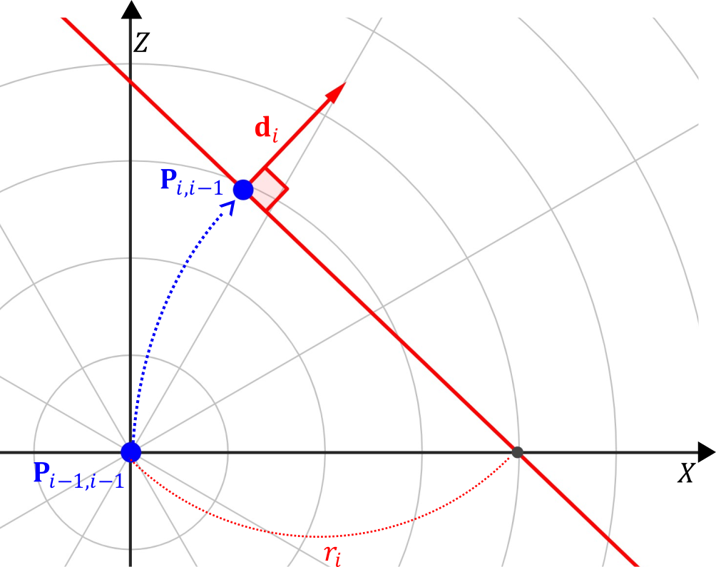
ignoring vertical movements as assumed above, where ${\mathbf{R}}_{i,i-1}$ is calculated as in Equation (11). Figure 2 shows the geometrical illustration of calculating ${\mathbf{d}}_{i}$ with the vehicle poses ${\mathbf{P}}_{i,0}$ and ${\mathbf{P}}_{i-1,0}$.

3.2.2 Calculating a Turning Radius

Second, we calculate the turning radius of the vehicle – i.e., the vehicle’s trajectory radius when it turns – at the $i$th time point, by using Equation (11) and (15). Consider again that the vehicle pose at the $(i-1)$th time point is ${\mathbf{I}}$; see the $X$-$Z$ vehicle coordinate system in Figure 2. In the $X$-$Z$ coordinate system, a line that is perpendicular to the directional vector ${\mathbf{d}}_{i}$ and crosses ${\mathbf{t}}_{i}$ is parameterized by

$$Z=-\frac{d_{i,Z}}{d_{i,X}}X+\left(t_{(i,i-1),Z}+\frac{d_{i,Z}}{d_{i,X}}t_{(i,i-1),X}\right),$$

where $d_{i,X}$ and $d_{i,Z}$ are the $X$- and $Z$-components of ${\mathbf{d}}_{i}$, respectively, and $t_{(i,i-1),X}$ and $t_{(i,i-1),Z}$ are the $X$- and $Z$-components of ${\mathbf{t}}_{i,i-1}$ (in (11)), respectively. We thus, obtain the turning radius of the vehicle at the $i$th time point (i.e., the $X$-intercept), $r_{i}$, as follows:

$$r_{i}=t_{(i,i-1),Z}\frac{d_{i,X}}{d_{i,Z}}+t_{(i,i-1),X}.$$ (16)

The sign of a turning radius indicates the turning direction: a positive and negative number indicates a right and left turn, respectively. Figure 2 illustrates the relations between the $i$th turning radius, $i$th forward vehicle vector, and the $i$th and $(i-1)$th vehicle poses in the $X-Z$ vehicle coordinate system.

3.2.3 Calculating a Steering Angle

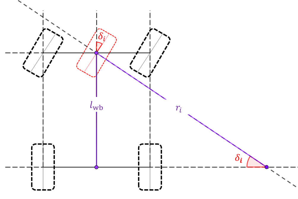
Finally, we estimate a steering angle for each time point. We use the calculated turning ratio in Equation (16) and two additional information about the vehicle, the wheelbase and steering ratio. Throughout, we consider the parallel steering geometry, the most widely known steering geometry. Figure 3 illustrates the parallel steering geometry. Either using front-wheel or all-wheel drive, the parallel steering geometry for four-wheeled vehicles turns both front wheels by the same amount.¹⁶ For simplicity of illustration, we consider front-wheel drive for four-wheeled vehicles.

Let $l_{\text{wb}}$ be the wheelbase of the vehicle, the distance between the centers of the front and rear axles. Using the parallel steering geometry in Figure 3, we compute the degree of a front wheel turn $\delta_{i}$ at the $i$th time point as follows:

$$\delta_{i}=\arcsin\!\left(\frac{l_{\text{wb}}}{r_{i}}\right)$$ (17)

where ${r}_{i}$ is calculated as in Equation (16), and both $l_{\text{wb}}$ and $r_{i}$ are in the same unit.

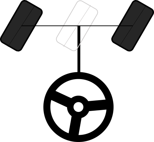
There exists some difference between a steering wheel angle and a front wheel turn angle (as illustrated in Figure 4). This relation, so-called steering ratio, is a unique parameter of a vehicle:

$$\text{steering ratio}=\frac{y_{i}}{\delta_{i}},$$

where $y_{i}$ is the steering wheel angle at the $i$th time point, and $\delta_{i}$ is given as in Equation (17). Using this unique parameter of a vehicle and $\delta_{i}$ in Equation (17), we finally obtain a pseudo steering angle $\hat{y}$ at the $i$th time point (see Figure 1) by

$$\hat{y}=\text{steering ratio}\times\delta_{i}$$ (18)

In sum, using the pseudo labels in Equation (18), we can train an E2E driving NN (in a self-supervised manner) that gives a steering angle for each time point from an image captured by a camera. In obtaining the pseudo labels, we use domain knowledge of the vehicle, including vehicle poses, steering geometry, wheelbase, and steering ratio.

4 Experimental Results and Discussion

This section compares the performances of E2E driving NNs trained by the ordinary SIL⁶ and the proposed SSIL framework, for three different driving scene datasets and two different NN architectures. In addition, this section interprets E2E driving NNs trained via SIL and SSIL, by generating and comparing their saliency maps.

4.1 Experimental Setups

4.1.1 Datasets

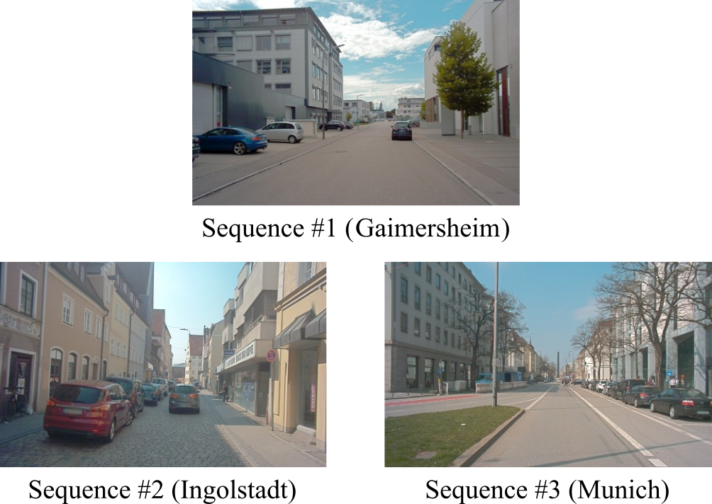
We used the A2D2 data¹⁸ that for each frame, includes images collected from cameras, point cloud sets from LiDAR sensors, human driving commands, etc. The A2D2 data consists of three driving scenes that were collected in different cities in Germany, Gaimersheim, Ingolstadt, and Munich, and Figure 5 shows examples of three driving scenes. The Gainmersheim dataset was acquired in rural areas, where roads and sidewalks are distinct and lanes exist intermittently. The Ingolstadt dataset was acquired in narrow alleys where roads and sidewalks are indistinguishable and lanes exist intermittently. The Munich dataset was acquired from main road in urban area with various buildings and visible lanes in most frames. We denote the Gaimersheim, Ingolstadt, and Munich datasets as Sequence #1, #2, and #3, respectively.

In each driving sequence, we used 1) images collected from a camera at the center of the front header (“front-center camera”), 2) point clouds from LiDAR sensors at the left, center, and right of the front header (“front-left, front-center, and front-right LiDAR,” respectively), and 3) the human driven steering angle values. We changed the spatial resolution of input RGB images to $320\times 160$ and to better focus on road scene, we cut $65$ and $25$ pixels from the top and bottom, respectively.

To accumulate sufficient point clouds for accurate pose estimation, we divided each dataset into fixed windows of $15$ seconds ($450$ frames). We divided Sequences #1, #2, and #3 into $27$, $33$, and $35$ chunks, respectively (with the total number of time points is $12,\!600$, $14,\!850$, and $15,\!750$, respectively). We used $80$% and $20$% of chunks for training and test, respectively. We expect that this scheme is more reasonable to test the generalization capability of trained E2E driving NNs than randomly selecting frames that leads to higher similarity between training and test datasets.

4.1.2 Vehicle Information

The A2D2 data was collected by the Audi Q7 e-tron model. The wheelbase of the vehicle $l_{\text{wb}}$ in Equation (17) is $2.994$m and its steering ratio in Equation (18) is $15.8$. The vehicle uses the all-wheel drive system.

4.1.3 E2E Driving NN Architectures

Throughout performance comparison experiments with different learning methods and driving sequences, we used two feature extraction architectures: PilotNet⁶ and PilotNet using the widely known recurrent neural network, long short term memory (LSTM) network. Since feature extraction network architecture is the representative difference between the two, we will refer them to as “convolutional neural network (CNN)” and “CNN+LSTM”.

We used the PilotNet architecture (called “CNN” throughout) as is in ⁶. It consists of one normalization layer, five convolutional layers with the kernel sizes of $5\times 5$, $5\times 5$, $5\times 5$, $3\times 3$, and $3\times 3$ (from the first to the fifth layer), and four fully-connected (FC) layers with the numbers of neurons of $100$, $50$, $10$, and $1$

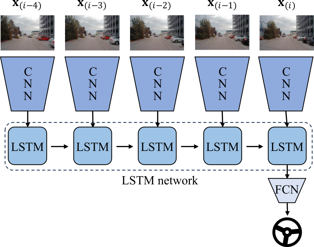
Figure 6 illustrates the overall architecture of “CNN+LSTM”. We designed it to additionally use temporal information in five time points, $\{i,i-1,i-2,i-3,i-4\}$. We used the feature extraction CNN architecture of PilotNet to extract a feature map for each time point (of which parameters are shared across all time points). We constructed the LSTM network in a many-to-one manner, where we set the dimension of the hidden state (i.e., hidden size) as $128$ for each cell. We used a single-layer FC network to predict a steering angle by taking as input the LSTM network output using features extracted from five time points.

4.1.4 A Choice Between LOAM and A-LOAM

To choose a better pseudo-label predictor for SSIL, we evaluated LOAM and A-LOAM in terms of the pseudo-label prediction performance. We calculated mean squared error (MSE) between their predicted pseudo steering angles via the proposed method in Section 3 and the ground-truth values. Comparing the results in Table 1 for different driving sequences shows that A-LOAM improves the pseudo-label prediction performance over LOAM. This is because A-LOAM is more efficient than LOAM and the performance of simultaneous localization and mapping (SLAM) methods depends on the execution time.

Based on the expected prediction error analysis in Section 2 and the results in Table 1, we chose A-LOAM over LOAM throughout our SSIL experiments. Note that we compared A-LOAM and LOAM only for selecting a better pseudo-label predictor for SSIL. In the inference stage, we only use images collected from a camera, but not LiDAR sensors. (In SSIL, we used both camera and LiDAR sensors, as described in Section 3.)

4.1.5 Training

We first finely tuned the training hyperparameters to obtain the best inference accuracy for SIL using the CNN architecture. We used them throughout all learning methods and NN architectures: we set the initial learning rate, the batch size and the number of epochs as $0.0001$, $16$ and $100$, respectively. To make sure that the loss functions converge within $100$ epochs, we decayed the learning rate by a factor of $0.9$ at every $60$ epochs.

We do not know the exact distribution of $x$ in expected loss Euqation (1), so as conventionally, we approximated it to the empirical SSIL loss function $\sum_{l=1}^{L}\|f(({\mathbf{x}}_{l})_{J^{c}})-g(({\mathbf{x}}_{l})_{J})\|_{2}^{2}$, where $({\mathbf{x}}_{l})_{J^{c}}$ and $({\mathbf{x}}_{l})_{J}$ are an image and point clouds at the $l$th frame, respectively, and $L$ is the number of training samples. We pre-computed a pseudo steering angle for each frame by $\hat{y}_{l}=g(({\mathbf{x}}_{l})_{J})$, for $l=1,\ldots,L$, so that training times of SIL and SSIL models are identical, given the same NN architecture.

In training CNN+LSTM models, to use a similar number of training instances as used in training CNN models, we used $80$% overlap between each training instance.

4.1.6 Evaluation Metric

Throughout, we used the conventional steering angle prediction measure MSE.⁶ We averaged MSE values from all folds in 5-fold cross validation.

4.2 Comparisons between SIL and SSIL

Regardless of driving sequences and NN architectures, Table 2 and Figure 7 demonstrate that without using expert driving commands, an E2E driving NN trained by proposed SSIL achieves very comparable performance with that of ordinary SIL. Even in Sequence #2 that seems more challenging for autonomous driving than Sequences #1 & #3 (see their driving circumstances in Section 4.1.1), SSIL without using human driving commands can achieve comparable E2E driving performance with SIL.

We did not observe the performance improvement by using the CNN+LSTM feature extractor in Figure 6 over the existing CNN feature extractor.⁶

4.3 Visualization of the Feature Map for Supervised and Self-Supervised

This section qualitatively analyzes SIL and SSIL using saliency maps generated by the VisualBackProp method.¹⁷ (VisualBackProp was used for explaining the performance of PilotNet.⁶) Using VisualBackProp, we measure the degree of importance of a pixel for each model to predict a steering angle. Figure 8 compares saliency maps between SIL and SSIL for six different driving scenes: Figure 8a and 8b show saliency maps of the same driving scenes for SIL and SSIL, respectively. Not surprisingly, trained E2E driving NNs by proposed SSIL and ordinary SIL emphasize similar areas of an image that contribute to predictions. In the first and second driving scenes in Figure 8, both E2E driving NNs attend vehicles in a parking lot next to the building on the left and barrier curbs. In the third and fourth driving scenes in Figure 8, both trained NNs pay attention to vehicles in a parking lot next to the building on the right and barrier curbs. In the fifth driving scene in Figure 8, they mostly “see” fences and the sidewalk/barrier curbs ahead. In the sixth driving scene in Figure 8, both trained NNs via SIL and SSIL focuses on the building and sidewalk on the left. In sum, E2E driving NNs trained by proposed SSIL and the supervision counterpart attend similar objects in making predictions. These saliency map comparison results well correspond to the numerical results in Section 4.2.

5 Limitations

This section discusses two limitations of the proposed SSIL framework. First, SSIL depends on the performance of SLAM for pseudo-label prediction. The proposed method in Section 3 uses a SLAM method using LiDAR data, (A-)LOAM,¹⁹ and its performance intrinsically depends on the quality of LiDAR data. LiDAR sensors are known to be susceptible to range errors, reflection errors, etc. that are caused by various environments including reflective surfaces (e.g., glass/metal and bright sunlight), physical obstructions depending on weather conditions (e.g., heavy rain, fog, and snow).^{20; 21; 22; 23; 24} Those errors could degrade the quality of LiDAR data and when they exist, it is more challenging to design an effective pseudo-label predictor.

Second, a trained E2E driving NN by proposed SSIL may be only suboptimal for vehicles with different intrinsic vehicle parameters. The proposed SSIL framework uses domain knowledge of sensors and a vehicle, e.g., LiDAR intrinsic/extrinsic parameters for LOAM in Section 3.1, wheelbase in Equation (17), steering ratio Equation (18). In particular, steering ratio is an intrinsic parameter to a vehicle, so if a vehicle changes with one with a different steering ratio, one needs to re-predict pseudo labels for SSIL of an E2E driving NN.

6 Conclusion

In training E2E driving networks, it is crucial to construct vehicle control datasets. However, it is extremely challenging to access such vehicle data, e.g., steering angle control, without the assistance of vehicle manufacturers. To address this challenge, we propose the SSIL framework that can predict pseudo steering angles using a camera and three LiDAR sensors. Our experimental results and saliency map analyses demonstrate that the proposed SSIL framework can achieve very comparable performance with that of ordinary SIL.

Our first future work is to extend the the proposed SSIL framework to construct pseudo labels for other driving commands, such as velocity and brake throttle, using the proposed vehicle forward direction estimation in Section 3.2.1. Our second future work is to overcome the aforementioned limitation of LiDAR sensors (in Section 5) by a SLAM method²⁵ that can compensate for weaknesses of each sensor, e.g., a monocular camera and a LiDAR sensor, using both camera and LiDAR data. We will design effective pseudo-label predictors for SSIL of E2E driving networks that can estimate more diverse driving commands and be robustly adaptable to various driving environments.

Acknowledgements

J. B. Park and J. Lee equally contributed to this work. The work of J. B. Park and I. Y. Chun was supported in part by NRF grants 2022R1F1A1074546 and RS-2023-00213455 funded by MSIT, KIAT grant P0022098 funded by MOTIE, and the BK21 FOUR Project. The work of I. Y. Chun was additionally supported in part by IITP grant 2019-0-00421 funded by MSIT, IBS grant R015-D1, the KEIT Technology Innovation program grant 20014967 funded by MOTIE, the IITP Information Technology Research Center program grant 2023-2018-0-01798 funded by MSIT, SKKU-SMC and SKKU-KBSMC Future Convergence Research Program grants, and SKKU seed grants. The work of D. Ma was supported by the project 2020-2-TCS funded by the Hawaii DOT. The work of S. M. Won was supported by the IITP ICT Creative Consilience program grant 2020-0-01821 funded by MSIT.

Conflict of Interest

The authors declare no conflict of interest.

Figure 1: Overview of the proposed SSIL framework. We modify the general self-supervised regression learning framework¹⁵ by designing a pseudo-label predictor using domain knowledge. We designed it as the composition of a vehicle pose estimator using point clouds ${\mathbf{x}}_{J}$ generated from three LiDAR sensors, and a pseudo steering angle predictor. In comparing SSIL with the ordinary supervised learning method, we tested two E2E driving network architectures, one without a recurrent NN and the other with it. To train an E2E driving network that takes a camera image ${\mathbf{x}}_{J^{c}}$ as input and predicts a steering angle, a loss function measures the discrepancy between pseudo target $\hat{y}$ and the predicted steering angle.

Figure 2: Geometric illustration of calculating the turning radius in the $X$-$Z$ vehicle coordinate system where ${\mathbf{P}}_{i-1,i-1}={\mathbf{I}}$. The matrices ${\mathbf{P}}_{i,i-1}$ and ${\mathbf{P}}_{i-1,i-1}$ indicate the vehicle poses at the current and previous time points, respectively. The vector ${\mathbf{d}}_{i}$ indicates the forward direction vector of the vehicle at the current time point. The distance $r_{i}$ is a turning radius of the vehicle at the $i$th time point. It is given by the $X$-intercept of the line that is perpendicular to ${\mathbf{d}}_{i}$ and crosses ${\mathbf{t}}_{i,i-1}$ (the translation vector of ${\mathbf{P}}_{i,i-1}$) in the $X$-$Z$ vehicle coordinate system. The blue dotted arrow indicates a driving trajectory from the $(i-1)$th to $i$th time point.

Figure 3: The parallel steering geometry¹⁶ for four-wheeled vehicles using front-wheel drive. We set ${l}_{\text{wb}}$ as the actual wheelbase of the vehicle, and calculate $r_{i}$ as in Equation (16). In calculating $\delta_{i}$, we consider $l_{\text{wb}}$ and $r_{i}$ as the length of the opposite side and the length of the hypotenuse, respectively.

Figure 4: Steering wheel and front wheels. There exists a specific relation between steering wheel and front wheel angles.

Figure 5: Representative examples of three different driving sequences.

Figure 6: The E2E driving NN architecture using a recurrent NN to incorporate time information from the current time point $i$ and previous four time points $\{i-1,i-2,i-3,i-4\}$. FCN denotes a FC network.

Table 1: Pseudo target steering angle prediction accuracy comparisons between LOAM and A-LOAM for different driving sequences (MSE)

Driving scenes	LOAM	A-LOAM
Seq. #1	0.00320	0.00003
Seq. #2	0.01374	0.00023
Seq. #3	0.00367	0.00021

Table 2: E2E driving accuracy comparisons between SIL and SSIL for different driving sequences and feature extraction architectures (averaged MSE with $5$-fold cross validation for steering angle control)

Feat. extn. architectures	Seq. #1		Seq. #2		Seq. #3
	SIL	SSIL	SIL	SSIL	SIL	SSIL
CNN	0.024	0.027	0.0159	0.0152	0.013	0.015
CNN+LSTM	0.028	0.027	0.0158	0.0161	0.0127	0.0126

Figure 7: E2E driving accuracy comparisons between SIL and SSIL for different driving sequences and feature extraction architectures (averaged MSE with $5$-fold cross validation for steering angle control).

Figure 8: Saliency map comparisons between E2E driving NNs trained by SIL and SSIL (the degree of importance of a pixel to a NN to make the prediction increases from blue to green to yellow to red). (a) Examples of trained E2E driving NN via SIL. (b) Examples of trained E2E driving NN via SSIL. We used CNN+LSTM feature extractor for Sequence #1.

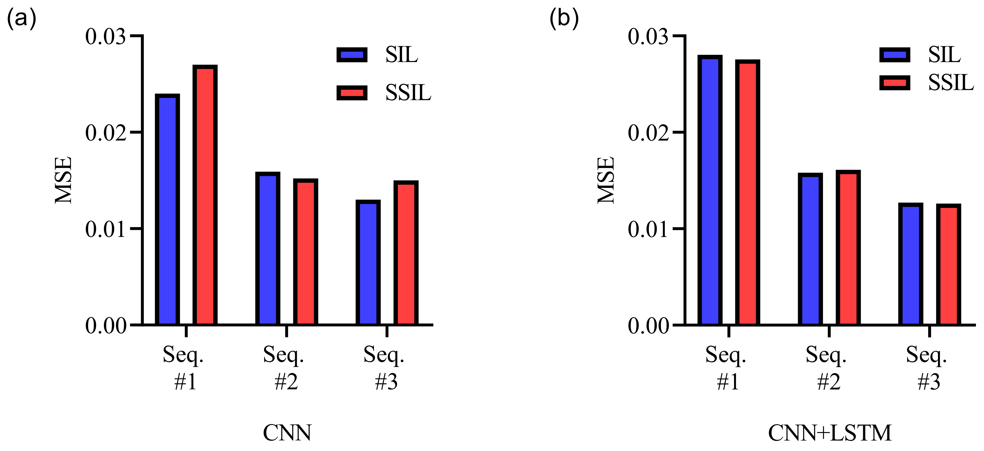
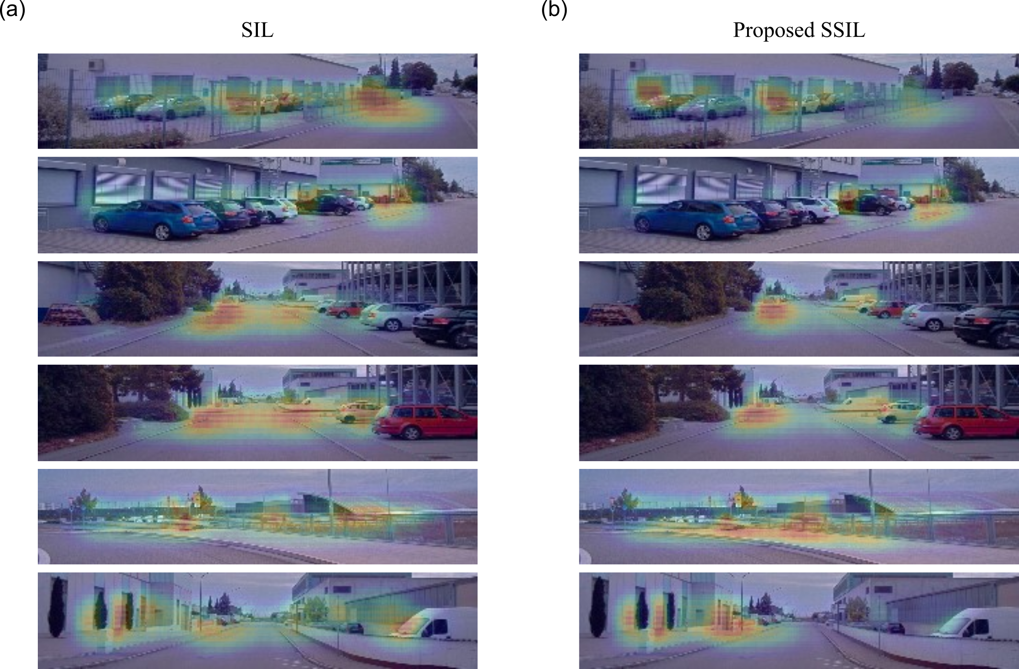
Table of Contents

The proposed self-supervised imitation learning framework can learn end-to-end autonomous driving neural networks without human driving commands. To predict pseudo steering angles, the proposed method uses a camera and three LiDAR sensors, and domain knowledge of LiDAR sensors and vehicle/steering geometry. Experiments and analysis demonstrate that the proposed framework achieves comparable autonomous driving accuracy with the supervision counterpart.

References

- [1] A. Tampuu, T. Matiisen, M. Semikin, D. Fishman, N. Muhammad, IEEE Trans. Neural Netw. Learn. Syst. 2022, 33, 4 1364.
- [2] D. Coelho, M. Oliveira, IEEE Access 2022, 10 75296.
- [3] E. Yurtsever, J. Lambert, A. Carballo, K. Takeda, IEEE Access 2020, 8 58443.
- [4] W. Zeng, W. Luo, S. Suo, A. Sadat, B. Yang, S. Casas, R. Urtasun, In Proc. IEEE Conf. Comput. Vis. Pattern Recognit. 2019 8660–8669.
- [5] D. A. Pomerleau, In Proc. Int. Conf. Neural Inf. Process. Syst. 1988 305–313.
- [6] M. Bojarski, D. D. Testa, D. Dworakowski, B. Firner, B. Flepp, P. Goyal, L. D. Jackel, M. Monfort, U. Muller, J. Zhang, X. Zhang, J. Zhao, K. Zieba, (Preprint) arXiv:1604.07316 2016.
- [7] T. Agarwal, H. Arora, J. Schneider, In Proc. IEEE Int. Intell. Transp. Syst. Conf. 2021 607–614.
- [8] F. Codevilla, M. Müller, A. López, V. Koltun, A. Dosovitskiy, In Proc. IEEE Int. Conf. Robot. Autom. 2018 4693–4700.
- [9] J. Hawke, R. Shen, C. Gurau, S. Sharma, D. Reda, N. Nikolov, P. Mazur, S. Micklethwaite, N. Griffiths, A. Shah, A. Kndall, In Proc. IEEE Int. Conf. Robot. Autom. 2020 251–257.
- [10] B. Osiński, A. Jakubowski, P. Zięcina, P. Miłoś, C. Galias, S. Homoceanu, H. Michalewski, In Proc. IEEE Int. Conf. Robot. Autom. 2020 6411–6418.
- [11] A. Kendall, J. Hawke, D. Janz, P. Mazur, D. Reda, J.-M. Allen, V.-D. Lam, A. Bewley, A. Shah, In Proc. IEEE Int. Conf. Robot. Autom. 2019 8248–8254.
- [12] B. D. Argall, S. Chernova, M. Veloso, B. Browning, Robot. Auton. Syst. 2009, 57, 5 469.
- [13] H. A. Ignatious, Hesham-El-Sayed, M. Khan, Procedia Comput. Sci. 2022, 198 736.
- [14] J. Kocić, N. Jovičić, V. Drndarević, In Proc. IEEE Telecom. Forum. 2018 420–425.
- [15] I. Y. Chun, D. Park, X. Zheng, S. Y. Chun, Y. Long, (Preprint) arXiv:2205.04832 2022.
- [16] R. N. Jazar, Vehicle Dynamics, volume 1, Springer, 2008.
- [17] M. Bojarski, A. Choromanska, K. Choromanski, B. Firner, L. J. Ackel, U. Muller, P. Yeres, K. Zieba, In Proc. IEEE Int. Conf. Robot. Autom. 2018 4701–4708.
- [18] J. Geyer, Y. Kassahun, M. Mahmudi, X. Ricou, R. Durgesh, A. S. Chung, L. Hauswald, V. H. Pham, M. Mühlegg, S. Dorn, T. Fernandez, M. Jänicke, S. Mirashi, C. Savani, M. Sturm, O. Vorobiov, M. Oelker, S. Garreis, P. Schuberth, (Preprint) arXiv:2004.06320 2020.
- [19] J. Zhang, S. Singh, In Proc. Robot. Sci. Syst., 9. 2014 1–9.
- [20] N. Charron, S. Phillips, S. L. Waslander, In Proc. Conf. Comput. Robot Vis. 2018 254–261.
- [21] M.-H. Le, C.-H. Cheng, D.-G. Liu, Electronics 2023, 12, 9 2150.
- [22] R. Heinzler, P. Schindler, J. Seekircher, W. Ritter, W. Stork, In Proc. IEEE Intell. Veh. Symp. 2019 1527–1534.
- [23] A. Filgueira, H. González-Jorge, S. Lagüela, L. Díaz-Vilariño, P. Arias, Measurement 2017, 95 143.
- [24] J. R. V. Rivero, I. Tahiraj, O. Schubert, C. Glassl, B. Buschardt, M. Berk, J. Chen, In Proc. IEEE Int. Intell. Transp. Syst. Conf. 2017 1–6.
- [25] J. Zhang, S. Singh, In Proc. Int. Conf. Robot. Autom. 2015 2174–2181.