The Nesterov–Spokoiny Acceleration Achieves Strict o(1/k²) Convergence

Abstract

We study a variant of an accelerated gradient algorithm of Nesterov and Spokoiny. We call this algorithm the Nesterov–Spokoiny Acceleration (NSA). The NSA algorithm simultaneously satisfies the following property: For a smooth convex objective $f\in\mathscr{F}_{L}^{\infty,1}(\mathbb{R}^{n})$, the sequence $\{\mathbf{x}_{k}\}_{k\in\mathbb{N}}$ governed by NSA satisfies $\limsup\limits_{k\to\infty}k^{2}(f(\mathbf{x}_{k})-f^{*})=0$, where $f^{*}>-\infty$ is the minimum of $f$.

1 Introduction

A central problem in optimization and related fields is solving

$$\min_{\mathbf{x}\in\mathbb{R}^{n}}f(\mathbf{x}),$$ (1)

where $f$ is a real-valued convex function bounded from below. An efficient solver for (1) has important real-world implications, since (1) captures the core challenge of many problems, ranging from systems control Lewis et al., (2012) to neural network training Goodfellow et al., (2016).

Over the years, gradient algorithms have become the default solver for (1) in several scenarios, and a tremendous among of gradient methods have been invented. The history of gradient algorithms dates back to classical times, when Cauchy proposed a method of finding the minimum value of a function via first-order information Lemaréchal, (2012).

Based on a common physics phenomenon and the original Gradient Algorithm, Polyak’s Heavy-ball method was invented Polyak, (1964). This algorithm is perhaps the first method that directly aims to accelerate the convergence of gradient search. One of the most surprising works in this field is the Nesterov’s Accelerated Gradient (NAG) method Nesterov, (1983), where accelerated gradient methods were invented to speed up the convergence for smooth convex programs. For such problems, NAG achieves a $O(k^{-2})$ convergence rate, without incurring computations of higher expense. When the iteration counter $k$ is not large, the convergence rate of NAG is proved to be optimal among methods where the next iteration can be written as a linear combination of previous gradients and the starting point Nesterov, (2004, 2018).

1.1 Accelerated Gradient Methods

Since Nesterov’s original acceleration method Nesterov, (1983), several accelerated gradient methods have been invented, including the one that inspires our work Nesterov, (2011); Nesterov and Spokoiny, (2017). Also, Flammarion and Bach, (2015) builds a connection between average gradient and acceleration. The nature of the acceleration phenomenon has also been investigated from a continuous-time perspective. In particular, Su et al., (2016) pointed out the relation between the a second-order ordinary differential equation and NAG. This discovery allows for a better understanding of Nesterov’s scheme. Afterwards, a family of schemes with $O(1/k^{2})$ convergence rates has been obtained. Shi et al., (2022) finds a finer correspondence between discrete-time iteration and continuous-time trajectory and proposes a gradient-correction scheme of NAG. Chen et al., (2022) introduced an implicit-velocity scheme of NAG and investigates on the convergence rate of gradient norms. Please See Section 4.1.1 for more discussions on the continuous-time perspective.

Accelerated proximal methods have also been studied extensively; See e.g., Parikh et al., (2014) for an exposition. A primary motivations for proximal methods is possible nonsmoothness in the objective. Roughly speaking, the proximal operator finds the next iteration point by minimizing an approximation of the objective (or part of the objective) plus a regularizer term. In a broad sense, the mirror map in mirror descent Nemirovsky and Yudin, (1983) is also a type of proximal operator. In discussing related works, mirror descent algorithms are considered as proximal methods.

Although some authors view gradient methods (such as gradient descent) as special cases of proximal method (e.g., Beck and Teboulle, (2009)), we make a clear distinction between gradient methods and proximal methods. The reasons are two-fold: 1. For important real-world tasks such as neural network training Goodfellow et al., (2016), typical proximal operators are more expensive than gradient methods, since they involve solving a subproblem at each step. 2. The proximal operation, as per defined in some prior arts, cannot be reduced to a gradient method even if smoothness condition is imposed, since it implicitly uses the (sub-)gradient at $\mathbf{x}_{k+1}$ to arrive at $\mathbf{x}_{k+1}$.

Over the years, various accelerated proximal methods have been invented. Nesterov, (2005) introduced a proximal method that achieves $O(k^{-2})$ convergence rate for convex nonsmooth programs. Beck and Teboulle, (2009) popularized accelerated proximal methods via the Fast Iterative Shrinkage-Thresholding Algorithm (FISTA) algorithm, which achieves a better rate of convergence for linear inverse problems, while preserving the computational simplicity of ISTA Combettes and Wajs, (2005); Daubechies et al., (2004). FISTA has also been analyzed in Chambolle and Dossal, (2015). Motivated by the complementary performances of mirror descent and gradient descent, Allen-Zhu and Orecchia, 2014a ; Diakonikolas and Orecchia, (2019) couple these two celebrated algorithms and present a new scheme to reconstruct NAG on the basis of other algorithms. Krichene et al., 2015a builds a continuous-time analysis of the accelerated mirror descent method, whose discretized version also converges at rate $O(\frac{1}{k^{2}})$. Bubeck et al., (2015) introduced a modification of NAG with a geometric interpretation and a proof of the same convergence rate as NAG. Notably, based on Nesterov’s forward backward method Attouch et al., (2014), Attouch and Peypouquet, (2016); Attouch, Hedy et al., (2019) invented an accelerated proximal methods that converges at rate $o(k^{-2})$.

Till now, this $o(k^{-2})$ convergence rate is achieved only by Attouch and Peypouquet, (2016). In this work, we introduce a variant of an acceleration method of Nesterov and Spokoiny that also converges at rate $o(1/k^{2})$.

1.2 Our Contributions

In this paper, we study an acceleration gradient method called Nesterov–Spokoiny Acceleration (NSA), which is a variation of an acceleration method of Nesterov and Spokoiny Nesterov, (2011); Nesterov and Spokoiny, (2017). The NSA algorithm does not use a proximal operator, and satisfies the following properties:

1. The sequence $\{\mathbf{x}_{k}\}_{k\in\mathbb{N}}$ governed by NSA satisfies

   $$\limsup\limits_{k\to\infty}k^{2}(f(\mathbf{x}_{k})-f^{*})=0,$$

   where $f^{*}>-\infty$ is the minimum of the smooth convex function $f$.

2. The sequence $\{\mathbf{x}_{k}\}_{k\in\mathbb{N}}$ governed by NSA satisfies

   $$\liminf\limits_{k\to\infty}k^{2}\log k\log\log k(f(\mathbf{x}_{k})-f^{*})=0.$$

3. The sequence $\{\mathbf{y}_{k}\}_{k\in\mathbb{N}}$ governed by NSA satisfies

   $$\liminf\limits_{k\to\infty}k^{3}\log k\log\log k\|\nabla f(\mathbf{y}_{k})\|^{2}=0.$$

Comparison of NSA with state-of-the-art prior arts is summarized in Table 1.

Extensions of the NSA algorithm is also studied. In Section 3, we study a variation of the NSA algorithm that handles inexact gradient. In Section 3, we show that a zeroth-order variant of NSA also achieves $o(1/k^{2})$ convergence. In Section 4, we study a variation of the NSA algorithm that solves convex nonsmooth programs. A continuous-time analysis is also provided. Some more literature from the continuous-time perspective are discussed in Section 7.

	$\limsup$ convergence rate for function value	$\liminf$ convergence rate for function value	$\liminf$ convergence rate for gradient norm square
Nesterov, (1983)	$O(\frac{1}{k^{2}})$	$O(\frac{1}{k^{2}})$	$O(\frac{1}{k^{2}})$
Beck and Teboulle, (2009)	$O(\frac{1}{k^{2}})$	$O(\frac{1}{k^{2}})$	N/A
Allen-Zhu and Orecchia, 2014b	$O(\frac{1}{k^{2}})$	$O(\frac{1}{k^{2}})$	N/A
Flammarion and Bach, (2015)	$O(\frac{1}{k^{2}})$	$O(\frac{1}{k^{2}})$	$O(\frac{1}{k^{2}})$
Krichene et al., 2015a	$O(\frac{1}{k^{2}})$	$O(\frac{1}{k^{2}})$	$O(\frac{1}{k^{2}})$
Krichene et al., 2015b	$O(\frac{1}{k^{2}})$	$O(\frac{1}{k^{2}})$	N/A
Attouch and Peypouquet, (2016)	$o(\frac{1}{k^{2}})$	$o(\frac{1}{k^{2}})$	N/A
Nesterov and Spokoiny, (2017)	$O(\frac{1}{k^{2}})$	$O(\frac{1}{k^{2}})$	$O(\frac{1}{k^{2}})$
Diakonikolas and Orecchia, (2019)	$O(\frac{1}{k^{2}})$	$O(\frac{1}{k^{2}})$	$O(\frac{1}{k^{2}})$
Attouch, Hedy et al., (2019)	$o(\frac{1}{k^{2}})$	$o(\frac{1}{k^{2}})$	N/A
Attouch et al., (2022)	$O(\frac{1}{k^{2}})$	$O(\frac{1}{k^{2}})$	N/A
Shi et al., (2022)	$O(\frac{1}{k^{2}})$	$O(\frac{1}{k^{2}})$	$O(\frac{1}{k^{3}})$
Chen et al., (2022)	$O(\frac{1}{k^{2}})$	$O(\frac{1}{k^{2}})$	$o(\frac{1}{k^{3}})$
This work	$o(\frac{1}{k^{2}})$	$o(\frac{1}{k^{2}\log k\log\log k})$	$o(\frac{1}{k^{3}\log k\log\log k})$

Table 1: Comparison with state-of-the-art acceleration methods for convex programs, listed in chronological order. The third column for proximal methods that targets at nonsmooth objectives are filled in with “N/A”. Many of the existing works have other virtues. For example, some find fine physical formulations of the acceleration phenomenon Su et al., (2016); Shi et al., (2022); some build prime-dual interpretation of the acceleration phenomenon Allen-Zhu and Orecchia, 2014a ; Diakonikolas and Orecchia, (2019). Some handles nonsmooth objectives and composite optimization problems Beck and Teboulle, (2009); Attouch and Peypouquet, (2016); Attouch, Hedy et al., (2019). Yet in terms of convergence rate without proximal operators, the NSA algorithm studied in this paper is the best.

2 The Nesterov–Spokoiny Acceleration

The Nesterov–Spokoiny Acceleration algorithm is described in Algorithm 1.

Algorithm 1 Nesterov–Spokoiny Acceleration (NSA)

1:  Initialize: Pick $\mathbf{x}_{0}=\mathbf{z}_{0}\in\mathbb{R}^{n}$ (such that $\nabla f(\mathbf{x}_{0})\neq 0$.)

2:  for $k=0,1,2,\cdots,$ do

3:     Compute $\mathbf{y}_{k}=(1-\alpha_{k})\mathbf{x}_{k}+\alpha_{k}\mathbf{z}_{k}$, with $\alpha_{k}=\frac{p}{k+p}$ for some constant $p$.

4:     $\mathbf{x}_{k+1}^{\prime}=\mathbf{y}_{k}-\eta\nabla f(\mathbf{y}_{k})$. /* $\eta$ is the step size. */

5:     $\mathbf{x}_{k+1}^{\prime\prime}=\mathbf{x}_{k}-\eta\nabla f(\mathbf{x}_{k})$.

6:     $\mathbf{x}_{k+1}=\begin{cases}\mathbf{x}_{k+1}^{\prime},&\text{ if }f(\mathbf{x}_{k+1}^{\prime})\leq f(\mathbf{x}_{k+1}^{\prime\prime})\\ \mathbf{x}_{k+1}^{\prime\prime},&\text{ otherwise. }\end{cases}$

7:     $\mathbf{z}_{k+1}=\mathbf{z}_{k}-\frac{\eta}{\alpha_{k}}\nabla f(\mathbf{y}_{k})$.

8:  end for

Convergence guarantee for smooth convex objectives $\mathscr{F}_{L}^{1,1}(\mathbb{R}^{n})$ Nesterov, (2004, 2018) is in Theorem 1. For completeness, the definition of $\mathscr{F}_{L}^{1,1}(\mathbb{R}^{n})$ is included in the Appendix.

Theorem 1.

Instate all notations in Algorithm 1. Consider an objective function $f\in\mathscr{F}_{L}^{1,1}(\mathbb{R}^{n})$. Let $\eta\in(0,\frac{2}{3L}]$ and let $p\geq 3$. Let $\alpha_{k}=\frac{p}{k+p}$ for each $k\in\mathbb{N}$.

1. The NSA algorithm satisfies

   $$\limsup_{k\to\infty}k^{2}(f(\mathbf{x}_{k})-f^{*})=0,\quad\text{and}\quad\liminf_{k\to\infty}k^{2}\log k\log\log k(f(\mathbf{x}_{k})-f^{*})=0,$$

   where $f^{*}=\min_{\mathbf{x}\in\mathbb{R}^{n}}f(\mathbf{x})>-\infty$.

2. The NSA algorithm satisfies

   $$\liminf_{k\to\infty}k^{3}\log k\log\log k\|\nabla f(\mathbf{y}_{k})\|^{2}=0.$$

Next we prove Theorem 1. We start with Proposition 1 and Lemma 1.

Proposition 1.

Let $\{a_{n}\}_{n\in\mathbb{N}}$ be a nonnegative, nonincreasing sequence. If $\sum_{n=0}^{\infty}na_{n}<\infty$, then $\lim\limits_{n\to\infty}n^{2}a_{n}=0$.

Proof.

Since $\{a_{n}\}_{n\in\mathbb{N}}$ is nonnegative and $\sum_{n=0}^{\infty}na_{n}<\infty$, we have

$$\lim_{n\to\infty}\sum_{k=n}^{2n}ka_{k}=0.$$

Since $a_{n}$ is nonincreasing, we have, for any $n$, $\sum_{k=n}^{2n}ka_{k}\geq n^{2}a_{2n}=\frac{1}{4}(2n)^{2}a_{2n}$. This shows that $\lim\limits_{n\to\infty}(2n)^{2}a_{2n}=0$.

Similarly, we have $\lim\limits_{n\to\infty}\sum_{k=n}^{2n+1}ka_{k}=0$. Repeating the above arguments shows that $\lim\limits_{n\to\infty}(2n+1)^{2}a_{2n+1}=0$. Thus $\lim\limits_{n\to\infty}n^{2}a_{n}=0$. ∎

Lemma 1.

Let $f\in\mathscr{F}_{L}^{1,1}(\mathbb{R}^{n})$ and let $\eta\in(0,\frac{2}{3L}]$. Let $\mathbf{x}_{k},\mathbf{y}_{k}$ be governed by the NSA algorithm. Then for all $t=0,1,2,\cdots$, it holds that

$$\delta_{k+1}\leq\delta_{k}\quad\text{ and }\quad f(\mathbf{x}_{k+1})\leq f(\mathbf{y}_{k})-\frac{2\eta}{3}\|\nabla f(\mathbf{y}_{k})\|^{2},$$

where $\delta_{k}:=f(\mathbf{x}_{k})-f^{*}$ is introduced to avoid notation clutter.

Proof.

By $L$-smoothness of $f$, we know that

$$f(\mathbf{x}_{k+1}^{\prime})\leq \;f(\mathbf{y}_{k})+\nabla f(\mathbf{y}_{k})^{\top}\left(\mathbf{x}_{k+1}^{\prime}-\mathbf{y}_{k}\right)+\frac{L}{2}\|\mathbf{x}_{k+1}^{\prime}-\mathbf{y}_{k}\|^{2}$$

$$\leq \;f(\mathbf{y}_{k})+\left(-\eta+\frac{1}{2}L\eta^{2}\right)\|\nabla f(\mathbf{y}_{k})\|^{2}.$$

Since $\eta\in(0,\frac{2}{3L}]$, we know

$$f(\mathbf{x}_{k+1}^{\prime})\leq \;f(\mathbf{y}_{k})-\frac{2\eta}{3}\|\nabla f(\mathbf{y}_{k})\|^{2}.$$ (2)

Similarly, we have

$$f(\mathbf{x}_{k+1}^{\prime\prime})\leq f(\mathbf{x}_{k})-\frac{2\eta}{3}\|\nabla f(\mathbf{x}_{k})\|^{2}.$$ (3)

By (3), we know

$$\delta_{k+1}\leq f(\mathbf{x}_{k+1}^{\prime\prime})-f(\mathbf{x}^{*})\leq f(\mathbf{x}_{k})-f(\mathbf{x}^{*})=\delta_{k}.$$

By (2) we know

$$f(\mathbf{x}_{k+1})\leq f(\mathbf{x}_{k+1}^{\prime})\leq f(\mathbf{y}_{k})-\frac{2\eta}{3}\|\nabla f(\mathbf{y}_{k})\|^{2}.$$

∎

Proof of Theorem 1.

Define

$$\Delta_{k}=\frac{\gamma_{k}}{2}\left\|\mathbf{z}_{k}-\mathbf{x}^{*}\right\|^{2}+f(\mathbf{x}_{k})-f(\mathbf{x}^{*}),$$

where $\gamma_{k+1}=\frac{\alpha_{k}^{2}}{\eta}$ for all $t=0,1,\cdots$. Thus for any $t\geq 1$, we have

$$\Delta_{k+1}= \;\frac{\gamma_{k+1}}{2}\left\|\mathbf{z}_{k}-\frac{\eta}{\alpha_{k}}\nabla f(\mathbf{y}_{k})-\mathbf{x}^{*}\right\|^{2}+f(\mathbf{x}_{k+1})-f(\mathbf{x}^{*})$$

$$= \;\frac{\gamma_{k+1}}{2}\left\|\mathbf{z}_{k}-\mathbf{x}^{*}\right\|^{2}-\left<\frac{\eta\gamma_{k+1}}{\alpha_{k}}\nabla f(\mathbf{y}_{k}),\mathbf{z}_{k}-\mathbf{x}^{*}\right>+\frac{\gamma_{k+1}\eta^{2}}{2\alpha_{k}^{2}}\|\nabla f(\mathbf{y}_{k})\|^{2}+f(\mathbf{x}_{k+1})-f(\mathbf{x}^{*})$$

$$= \;\frac{\gamma_{k+1}}{2}\left\|\mathbf{z}_{k}-\mathbf{x}^{*}\right\|^{2}-\left<\alpha_{k}\nabla f(\mathbf{y}_{k}),\mathbf{z}_{k}-\mathbf{x}^{*}\right>+\frac{\eta}{2}\|\nabla f(\mathbf{y}_{k})\|^{2}+f(\mathbf{x}_{k+1})-f(\mathbf{x}^{*})$$

$$\leq \;\frac{\gamma_{k+1}}{2}\left\|\mathbf{z}_{k}-\mathbf{x}^{*}\right\|^{2}-\left<\alpha_{k}\nabla f(\mathbf{y}_{k}),\mathbf{z}_{k}-\mathbf{x}^{*}\right>+f(\mathbf{y}_{k})-\frac{\eta}{6}\|f(\mathbf{y}_{k})\|^{2}-f(\mathbf{x}^{*}),$$ (4)

where the last inequality follows from Lemma 1.

By the update rule, we have

$$\Delta_{k+1}\leq \;\frac{\gamma_{k+1}}{2}\left\|\mathbf{z}_{k}-\mathbf{x}^{*}\right\|^{2}-\alpha_{k}\left<{\nabla}f(\mathbf{y}_{k}),\mathbf{z}_{k}-\mathbf{x}^{*}\right>+f(\mathbf{y}_{k})-f(\mathbf{x}^{*})-\frac{\eta}{6}\|\nabla f(\mathbf{y}_{k})\|^{2}$$

$$= \;\frac{\gamma_{k+1}}{2}\left\|\mathbf{z}_{k}-\mathbf{x}^{*}\right\|^{2}+\left<{\nabla}f(\mathbf{y}_{k}),(1-\alpha_{k})\mathbf{x}_{k}+\alpha_{k}\mathbf{x}^{*}-\mathbf{y}_{k}\right>+f(\mathbf{y}_{k})-f(\mathbf{x}^{*})-\frac{\eta}{6}\|\nabla f(\mathbf{y}_{k})\|^{2}$$

$$\leq \;\frac{\gamma_{k+1}}{2}\left\|\mathbf{z}_{k}-\mathbf{x}^{*}\right\|^{2}+f((1-\alpha_{k})\mathbf{x}_{k}+\alpha_{k}\mathbf{x}^{*})-f(\mathbf{x}^{*})-\frac{\eta}{6}\|\nabla f(\mathbf{y}_{k})\|^{2}$$

$$\leq \;\frac{\gamma_{k+1}}{2}\left\|\mathbf{z}_{k}-\mathbf{x}^{*}\right\|^{2}+(1-\alpha_{k})f(\mathbf{x}_{k})+\alpha_{k}f(\mathbf{x}^{*})-f(\mathbf{x}^{*})-\frac{\eta}{6}\|\nabla f(\mathbf{y}_{k})\|^{2},$$ (5)

where the second line follows from the update rule $\mathbf{y}_{k}=(1-\alpha_{k})\mathbf{x}_{k}+\alpha_{k}\mathbf{z}_{k}$, and the last two lines follow from convexity of $f$.

Rearranging terms in (5) gives

$$\frac{\Delta_{k+1}}{\gamma_{k+1}}\leq \;\frac{\Delta_{k}}{\gamma_{k}}+\left(\frac{1}{\gamma_{k+1}}-\frac{\alpha_{k}}{\gamma_{k+1}}-\frac{1}{\gamma_{k}}\right)(f(\mathbf{x}_{k})-f(\mathbf{x}^{*}))-\frac{\eta}{6\gamma_{k+1}}\|\nabla f(\mathbf{y}_{k})\|^{2}$$ (6)

Since $\alpha_{k}=\frac{p}{k+p}$ for some $p\geq 3$, we have that

$$\frac{1}{\gamma_{k+1}}-\frac{\alpha_{k}}{\gamma_{k+1}}-\frac{1}{\gamma_{k}}= \;\frac{\eta(k+p)^{2}}{p^{2}}-\frac{\eta(k+p)}{p}-\frac{\eta(k+p-1)^{2}}{p^{2}}$$

$$= \;\eta\frac{\left(2-p\right)(k+p)-1}{p^{2}}\leq-\eta\frac{k+p}{p^{2}}.$$

Again write $\delta_{k}:=f(\mathbf{x}_{k})-f(\mathbf{x}^{*})$ for simplicity. Rearranging terms in (6) gives

$$\eta\frac{k+p}{p^{2}}\delta_{k}\leq\frac{\Delta_{k}}{\gamma_{k}}-\frac{\Delta_{k+1}}{\gamma_{k+1}},$$

and thus

$$\sum_{k=1}^{\infty}\frac{k+p}{p^{2}}\delta_{k}<\infty.$$ (7)

By Lemma 1, we know that $\{\delta_{k}\}_{k=1}^{\infty}$ is decreasing. Thus by Proposition 1, we know $\limsup\limits_{k\to\infty}k^{2}\delta_{k}=\lim\limits_{k\to\infty}k^{2}\delta_{k}=0$.

Now assume, in order to get a contradiction, that there exists $\mu>0$ such that $\delta_{k}\geq\frac{\mu}{k^{2}\log k\log\log k}$ for all $k\geq 3$. Then we have

$$\sum_{k=3}^{\infty}k\delta_{k}\geq\sum_{k=3}^{\infty}\frac{\mu}{k\log k\log\log k}=\infty,$$

which is a contradiction to (7). Therefore, no strictly positive $\mu$ lower bounds $\delta_{k}k^{2}\log k\log\log k$ for all $k\geq 3$, meaning that

$$\liminf_{k\to\infty}\delta_{k}k^{2}\log k\log\log k=0.$$ (8)

Now we concludes the proof of item 1.

For item 2 of Theorem 1, we again rearrange terms in (6) and take a summation to obtain

$$\sum_{k=1}^{\infty}(k+p)^{2}\|\nabla f(\mathbf{y}_{k})\|^{2}<\infty.$$

An argument that leads to (8) finishes the proof of item 2 in Theorem 1.

∎

3 The NSA Algorithm with Inexact Gradient Oracle

In practice, many learning scenarios only allow access to zeroth-order information of the objective function Larson et al., (2019). In such cases, we can estimate the gradient first Flaxman et al., (2005); Nesterov and Spokoiny, (2017); Feng and Wang, (2023); Wang, (2022) and then apply gradient algorithms to solve the problem. Such gradient estimators can be abstractly summarized as an inexact gradient oracle, defined as follows.

For a function $f$, a point $\mathbf{x}\in\mathbb{R}^{n}$, estimation accuracy $\epsilon$, and a randomness descriptor $\xi$, the (inexact) gradient oracle $\mathcal{G}$ with parameters $f$, $\mathbf{x}$, $\epsilon$ (written $\mathcal{G}(f,\mathbf{x},\epsilon;\xi)$) is a vector in $\mathbb{R}^{n}$ that satisfies:

1. For any $\mathbf{x}\in\mathbb{R}^{n}$, any $\epsilon\in[0,\infty)$, there exists a constant $C$ that does not dependent on $\epsilon$, such that $\left\|\mathbb{E}_{\xi}\left[\mathcal{G}(f,\mathbf{x},\epsilon;\xi)\right]-\nabla f(\mathbf{x})\right\|\leq C\epsilon$.

2. At any $\mathbf{x}\in\mathbb{R}^{n}$ such that $\nabla f(\mathbf{x})\neq 0$, there exists $\epsilon\in(0,\infty)$ such that

   $$\frac{3}{4}\|\mathcal{G}(f,\mathbf{x},\epsilon;\xi)\|^{2}\leq\left<\mathcal{G}(f,\mathbf{x},\epsilon;\xi),\nabla f(\mathbf{x})\right>\leq\frac{5}{4}\|\mathcal{G}(f,\mathbf{x},\epsilon;\xi)\|^{2}$$

   almost surely.

Such gradient oracle $\mathcal{G}$ can be guaranteed by zeroth-order information. Formal statements for these properties are in Theorems 2 and 3. Theorem 2 has been proved in the literature by different authors Flaxman et al., (2005); Nesterov and Spokoiny, (2017); Feng and Wang, (2023). The proof for 3 is deferred to Section 6, since the existence of gradient oracles satisfying properties (H1) and (H2) is not the main focus of the paper.

Theorem 2 (Flaxman et al., (2005); Nesterov and Spokoiny, (2017); Feng and Wang, (2023)).

Let the function $f$ be $L$-smooth. If at any $\mathbf{x}\in\mathbb{R}^{n}$, we can access the function value $f(\mathbf{x})$, then there exists an oracle $\mathcal{G}$ such that (1) $\mathcal{G}$ satisfies property (H1), and (2) $\mathcal{G}$ can be explicitly calculated.

Theorem 3.

Consider a function $f\in\mathscr{F}$, where $\mathscr{F}$ denotes Nesterov’s $\mathscr{F}$ functions Nesterov, (2004, 2018). If at any $\mathbf{x}\in\mathbb{R}^{n}$, we can access the function value $f(\mathbf{x})$, then there exists an oracle $\mathcal{G}$ such that (1) $\mathcal{G}$ satisfies property (H2), and (2) $\mathcal{G}$ can be explicitly calculated.

Algorithm 2 Nesterov–Spokoiny Acceleration (NSA) that handles in exact gradient

1:  Inputs: Gradient oracle $\mathcal{G}$. /* The gradient oracle $\mathcal{G}$ needs not be exact. */

2:  Initialize: Pick $\mathbf{x}_{0}=\mathbf{z}_{0}\in\mathbb{R}^{n}$ (such that $\nabla f(\mathbf{x}_{0})\neq 0$.)

3:  for $t=0,1,2,\cdots,$ do

4:     Compute $\mathbf{y}_{k}=(1-\alpha_{k})\mathbf{x}_{k}+\alpha_{k}\mathbf{z}_{k}$, with $\alpha_{k}=\frac{p}{k+p}$ for some constant $p$.

5:     Obtain possibly inexact and stochastic gradients $\mathbf{g}_{k}(\mathbf{x}_{k}):=\mathcal{G}(f,\mathbf{x}_{k},\epsilon_{k};\xi_{k})$ and $\mathbf{g}_{k}(\mathbf{y}_{k}):=\mathcal{G}(f,\mathbf{y}_{k},\epsilon_{k};\xi_{k}^{\prime})$.

6:     /* $\epsilon_{k}$ is the error of the gradient oracle at step $k$. $\xi_{k}$, $\xi_{k}^{\prime}$ describe possible randomness in the gradient oracle. If the gradient oracle is exact, then $\epsilon_{k}=0$ and $\mathcal{G}(f,\cdot,0;\xi)=\nabla f(\cdot)$ surely. */

7:     $\mathbf{x}_{k+1}^{\prime}=\mathbf{y}_{k}-2\eta\mathbf{g}_{k}(\mathbf{y}_{k})$. /* $\eta$ is the step size. */

8:     $\mathbf{x}_{k+1}^{\prime\prime}=\mathbf{x}_{k}-2\eta\mathbf{g}_{k}(\mathbf{x}_{k})$.

9:     $\mathbf{x}_{k+1}=\begin{cases}\mathbf{x}_{k+1}^{\prime},&\text{ if }f(\mathbf{x}_{k+1}^{\prime})\leq f(\mathbf{x}_{k+1}^{\prime\prime})\\ \mathbf{x}_{k+1}^{\prime\prime},&\text{ otherwise. }\end{cases}$

10:     $\mathbf{z}_{k+1}^{\prime}=\mathbf{z}_{k}-\frac{\eta}{\alpha_{k}}\mathbf{g}_{k}(\mathbf{y}_{k})$.

11:     $\begin{cases}\text{{Option I: }}\mathbf{z}_{k+1}=\mathbf{z}_{k+1}^{\prime}.\\ \text{{Option II: }}\mathbf{z}_{k+1}=\Pi_{\mathbb{B}_{\mu}}(\mathbf{z}_{k+1}^{\prime}),\text{where $\Pi_{\mathbb{B}_{\mu}}$ is the projection to the ball of radius $\mu$},\end{cases}$

12:      /* Option II is needed only when the gradient oracle is inexact. */

13:  end for

Theorem 4.

Instate all notations in Algorithm 2. Consider an objective function $f\in\mathscr{F}_{L}^{1,1}(\mathbb{R}^{n})$. Let $\eta\in(0,\frac{1}{2L}]$ and fix $p\geq 3$, and let $\alpha_{k}=\frac{p}{k+p}$ for each $t\in\mathbb{N}$. In cases where the gradient oracle $\mathcal{G}$ is inexact and possibly stochastic, then if (a) the gradient oracle satisfies properties (H1) and (H2), (b) the gradient error $\epsilon_{k}$ satisfies $\sum_{k=1}^{\infty}\frac{\epsilon_{k}}{\alpha_{k}}<\infty$, and (c) the minimizer $\mathbf{x}^{*}$ of $f$ satisfies $\mathbf{x}^{*}\in\mathbb{B}_{\mu}$, then the NSA algorithm with Option II satisfies

$$\limsup_{k\to\infty}k^{2}(f(\mathbf{x}_{k})-f(\mathbf{x}^{*}))=0\;\;\;a.s.,$$

and

$$\liminf_{k\to\infty}k^{2}\log k\log\log k(f(\mathbf{x}_{k})-f(\mathbf{x}^{*}))=0,\;\;\;a.s.$$

Below we prove Theorem 4.

Lemma 2.

Let $f\in\mathscr{F}_{L}^{1,1}(\mathbb{R}^{n})$ and let $\eta\in(0,\frac{1}{2L}]$. Let $\alpha_{k}=\frac{p}{k+p}$ for some $p>0$. Let $\mathbf{x}_{k}$ be governed by the NSA algorithm. If the gradient estimation oracle $\mathcal{G}$ satisfies properties (H1) and (H2), then there exists an error sequence $\{\epsilon_{k}\}_{k\in\mathbb{N}}$, such that $\sum_{k=1}^{\infty}\frac{\epsilon_{k}}{\alpha_{k}}<\infty$, and for all $k=0,1,2,\cdots$, it holds that

$$\delta_{k+1}\leq\delta_{k}\quad\text{ and }\quad f(\mathbf{x}_{k+1})\leq f(\mathbf{y}_{k})-\eta\|\mathbf{g}_{k}(\mathbf{y}_{k})\|^{2},$$

where $\delta_{k}:=f(\mathbf{x}_{k})-f(\mathbf{x}^{*})$ is introduced to avoid notation clutter.

Proof.

Since the gradient estimation oracle $\mathcal{G}$ satisfies property (H2), we know that, at any $\mathbf{y}_{k}$ with $\nabla f(\mathbf{y}_{k})\neq 0$, there exists $\epsilon^{\prime}>0$ such that

$$\frac{3}{4}\|\mathcal{G}(f,\mathbf{y}_{k},\epsilon^{\prime};\xi_{k}^{\prime})\|^{2}\leq\nabla f(\mathbf{x})^{\top}\mathcal{G}(f,\mathbf{y}_{k},\epsilon^{\prime};\xi_{k}^{\prime})\leq\frac{5}{4}\|\mathcal{G}(f,\mathbf{y}_{k},\epsilon^{\prime};\xi_{k}^{\prime})\|^{2},$$ (9)

almost surely. By letting $\epsilon_{k}$ to be smaller than this $\epsilon^{\prime}$, we have

$$\frac{3}{4}\|\mathbf{g}_{k}(\mathbf{y}_{k})\|^{2}\leq\nabla f(\mathbf{x})^{\top}\mathbf{g}_{k}(\mathbf{y}_{k})\leq\frac{5}{4}\|\mathbf{g}_{k}(\mathbf{y}_{k})\|^{2},\quad a.s.$$

Note that we can find a $\epsilon_{k}\leq\epsilon^{\prime}$ at any $k$ without violating $\sum_{k=1}^{\infty}\frac{\epsilon_{k}}{\alpha_{k}}<\infty$.

By $L$-smoothness of $f$, we know that

$$f(\mathbf{x}_{k+1}^{\prime})\leq \;f(\mathbf{y}_{k})+\nabla f(\mathbf{y}_{k})^{\top}\left(\mathbf{x}_{k+1}^{\prime}-\mathbf{y}_{k}\right)+\frac{L}{2}\|\mathbf{x}_{k+1}^{\prime}-\mathbf{y}_{k}\|^{2}$$

$$= \;f(\mathbf{y}_{k})-2\eta\nabla f(\mathbf{y}_{k})^{\top}\mathbf{g}_{k}(\mathbf{y}_{k})+2L\eta^{2}\|\mathbf{g}_{k}(\mathbf{y}_{k})\|^{2}$$

$$\leq \;f(\mathbf{y}_{k})+\left(-2\eta+2L\eta^{2}\right)\|\mathbf{g}_{k}(\mathbf{y}_{k})\|^{2},$$

where the last inequality follows from (9). Since $\eta\in(0,\frac{1}{2L}]$, we know

$$f(\mathbf{x}_{k+1}^{\prime})\leq \;f(\mathbf{y}_{k})-\eta\|\mathbf{g}_{k}(\mathbf{y}_{k})\|^{2}.$$ (10)

Similarly, we have

$$f(\mathbf{x}_{k+1}^{\prime\prime})\leq f(\mathbf{y}_{k})+\nabla f(\mathbf{y}_{k})^{\top}\left(\mathbf{x}_{k+1}^{\prime\prime}-\mathbf{y}_{k}\right)+\frac{L}{2}\|\mathbf{x}_{k+1}^{\prime\prime}-\mathbf{y}_{k}\|^{2}\leq f(\mathbf{x}_{k})-\eta\|\mathbf{g}_{k}(\mathbf{y}_{k})\|^{2}.$$ (11)

By (3), we know

$$\delta_{k+1}\leq f(\mathbf{x}_{k+1}^{\prime\prime})-f(\mathbf{x}^{*})\leq f(\mathbf{x}_{k})-f(\mathbf{x}^{*})=\delta_{k}.$$

By (2) we know

$$f(\mathbf{x}_{k+1})\leq f(\mathbf{x}_{k+1}^{\prime})\leq f(\mathbf{y}_{k})-\eta\|\mathbf{g}_{k}(\mathbf{y}_{k})\|^{2}.$$

∎

Lemma 3.

Instate all notations in Algorithm 2. Consider an objective function $f\in\mathscr{F}_{L}^{1,1}(\mathbb{R}^{n})$. Let $\alpha_{k}\in(0,1]$ for all $k\in\mathbb{N}$. Define $\gamma_{k+1}:=\frac{\alpha_{k}^{2}}{\eta}$ for all $k\geq 1$, and define

$$\Delta_{k}:=\frac{\gamma_{k}}{2}\|\mathbf{z}_{k}-\mathbf{x}^{*}\|^{2}+\delta_{k},$$

where $\delta_{k}:=f(\mathbf{x}_{k})-f^{*}$. For Algorithm 2 with Option II, if $\mathbf{x}^{*}\in\mathbb{B}_{\mu}$, then there exists a constant $C$ such that

$$\mathbb{E}\left[\left(\frac{1}{\gamma_{k}}+\frac{\alpha_{k}}{\gamma_{k+1}}-\frac{1}{\gamma_{k+1}}\right)\delta_{k}\right]\leq\mathbb{E}\left[\frac{\Delta_{k}}{\gamma_{k}}\right]-\mathbb{E}\left[\frac{\Delta_{k+1}}{\gamma_{k+1}}\right]+\frac{2C\mu\alpha_{k}\epsilon_{k}}{\gamma_{k+1}}$$

for all $k=1,2,\cdots$.

Proof.

For any $t\geq 1$, we have

$$\;\frac{\gamma_{k+1}}{2}\left\|\mathbf{z}_{k+1}^{\prime}-\mathbf{x}^{*}\right\|^{2}+f(\mathbf{x}_{k+1})-f(\mathbf{x}^{*})$$

$$= \;\frac{\gamma_{k+1}}{2}\left\|\mathbf{z}_{k}-\frac{\eta}{\alpha_{k}}\mathbf{g}_{k}(\mathbf{y}_{k})-\mathbf{x}^{*}\right\|^{2}+f(\mathbf{x}_{k+1})-f(\mathbf{x}^{*})$$

$$= \;\frac{\gamma_{k+1}}{2}\left\|\mathbf{z}_{k}-\mathbf{x}^{*}\right\|^{2}-\left<\frac{\eta\gamma_{k+1}}{\alpha_{k}}\mathbf{g}_{k}(\mathbf{y}_{k}),\mathbf{z}_{k}-\mathbf{x}^{*}\right>+\frac{\gamma_{k+1}\eta^{2}}{2\alpha_{k}^{2}}\|\mathbf{g}_{k}(\mathbf{y}_{k})\|^{2}+f(\mathbf{x}_{k+1})-f(\mathbf{x}^{*})$$

$$= \;\frac{\gamma_{k+1}}{2}\left\|\mathbf{z}_{k}-\mathbf{x}^{*}\right\|^{2}-\left<\alpha_{k}\mathbf{g}_{k}(\mathbf{y}_{k}),\mathbf{z}_{k}-\mathbf{x}^{*}\right>+\frac{\eta}{2}\|\mathbf{g}_{k}(\mathbf{y}_{k})\|^{2}+f(\mathbf{x}_{k+1})-f(\mathbf{x}^{*})$$

$$\leq \;\frac{\gamma_{k+1}}{2}\left\|\mathbf{z}_{k}-\mathbf{x}^{*}\right\|^{2}-\left<\alpha_{k}\mathbf{g}_{k}(\mathbf{y}_{k}),\mathbf{z}_{k}-\mathbf{x}^{*}\right>+f(\mathbf{y}_{k})-f(\mathbf{x}^{*}),$$

where the last inequality follows from Lemma 2.

If $\mathbf{x}^{*}\in\mathbb{B}_{\mu}$, then $\left\|\mathbf{z}_{k+1}-\mathbf{x}^{*}\right\|\leq\left\|\mathbf{z}_{k+1}^{\prime}-\mathbf{x}^{*}\right\|$. Thus

$$\Delta_{k+1}\leq\frac{\gamma_{k+1}}{2}\left\|\mathbf{z}_{k}-\mathbf{x}^{*}\right\|^{2}-\left<\alpha_{k}\mathbf{g}_{k}(\mathbf{y}_{k}),\mathbf{z}_{k}-\mathbf{x}^{*}\right>+f(\mathbf{y}_{k})-f(\mathbf{x}^{*}).$$

Let $\mathbb{E}_{k}$ be the expectation with respect to $\xi_{k}$ and $\xi_{k}^{\prime}$. Since $\mathcal{G}$ satisfies property (H1), taking expectation (with respect to $\xi_{k}$ and $\xi_{k}^{\prime}$) on both sides of the above inequality gives

$$\mathbb{E}_{k}\left[\Delta_{k+1}\right]\leq \;\frac{\gamma_{k+1}}{2}\left\|\mathbf{z}_{k}-\mathbf{x}^{*}\right\|^{2}-\alpha_{k}\left<{\nabla}f(\mathbf{y}_{k}),\mathbf{z}_{k}-\mathbf{x}^{*}\right>+C\alpha_{k}\epsilon_{k}\|\mathbf{z}_{k}-\mathbf{x}^{*}\|+f(\mathbf{y}_{k})-f(\mathbf{x}^{*}),$$

for some absolute constant $C$. Since $\mathbf{z}_{k}\in\mathbb{B}_{\mu}$ and $\mathbf{x}^{*}\in\mathbb{B}_{\mu}$, we know $\|\mathbf{z}_{k}-\mathbf{x}^{*}\|\leq 2\mu$, and thus

$$\mathbb{E}_{k}\left[\Delta_{k+1}\right]\leq \;\frac{\gamma_{k+1}}{2}\left\|\mathbf{z}_{k}-\mathbf{x}^{*}\right\|^{2}+\left<{\nabla}f(\mathbf{y}_{k}),(1-\alpha_{k})\mathbf{x}_{k}+\alpha_{k}\mathbf{x}^{*}-\mathbf{y}_{k}\right>+f(\mathbf{y}_{k})-f(\mathbf{x}^{*})+2C\mu\alpha_{k}\epsilon_{k}$$

$$\leq \;\frac{\gamma_{k+1}}{2}\left\|\mathbf{z}_{k}-\mathbf{x}^{*}\right\|^{2}+(1-\alpha_{k})(f(\mathbf{x}_{k})-f(\mathbf{x}^{*}))+2C\mu\alpha_{k}\epsilon_{k},$$

$$= \;\frac{\gamma_{k+1}}{\gamma_{k}}\Delta_{k}+\left(1-\alpha_{k}-\frac{\gamma_{k+1}}{\gamma_{k}}\right)(f(\mathbf{x}_{k})-f(\mathbf{x}^{*}))+2C\mu\alpha_{k}\epsilon_{k}.$$ (12)

where the second last line follows from convexity of $f$.

Then taking total expectation on both sides of (12) and rearranging terms gives

$$\mathbb{E}\left[\left(\frac{1}{\gamma_{k}}+\frac{\alpha_{k}}{\gamma_{k+1}}-\frac{1}{\gamma_{k+1}}\right)\delta_{k}\right]\leq\mathbb{E}\left[\frac{\Delta_{k}}{\gamma_{k}}\right]-\mathbb{E}\left[\frac{\Delta_{k+1}}{\gamma_{k+1}}\right]+\frac{2C\mu\alpha_{k}\epsilon_{k}}{\gamma_{k+1}}.$$

∎

Proof of Theorem 4.

Since $p\geq 3$, $\alpha_{k}=\frac{p}{k+p}$, and $\gamma_{k+1}=\frac{\alpha_{k}^{2}}{\eta}$, we have that

$$\frac{1}{\gamma_{k}}+\frac{\alpha_{k}}{\gamma_{k+1}}-\frac{1}{\gamma_{k+1}}\geq\eta\frac{k+p}{p^{2}}.$$

Since $\sum_{k=0}^{\infty}\frac{\epsilon_{k}}{\alpha_{k}}<\infty$, Lemma 3 implies

$$\mathbb{E}\left[\sum_{k=1}^{\infty}(k+p)\delta_{k}\right]<\infty.$$ (13)

Since $\mathbb{E}\left[\sum_{k=1}^{\infty}(k+p)\delta_{k}\right]<\infty$, $\sum_{k=1}^{\infty}(k+p)\delta_{k}<\infty$ almost surely. In addition, $\delta_{k}$ is nonnegative and decreasing (by Lemma 2). Therefore, by Proposition 1, we know that $\lim\limits_{k\to\infty}k^{2}(f(\mathbf{x}_{k})-f(\mathbf{x}^{*}))=0$ almost surely.

By (13), we know that

$$\mathbb{P}\left(\sum_{k=1}^{\infty}(k+p)\delta_{k}<\infty\right)=1.$$ (14)

Now, fix $\kappa\in\mathbb{Q}_{+}$ and consider the event

$$\mathcal{E}_{\kappa}=\left\{\delta_{k}\geq\frac{\kappa}{k^{2}\log k\log\log k},\;\text{ for all }k=2,3,\cdots\right\}.$$

Suppose, in order to get a contradiction, that there exists $\beta>0$ such that

$$\mathbb{P}\left(\mathcal{E}_{\kappa}\right)>\beta.$$ (15)

When $\mathcal{E}_{\kappa}$ is true, we know that

$$\sum_{k=2}^{\infty}(k+p)\delta_{k}\geq\sum_{k=2}^{\infty}\frac{\kappa}{k\log k\log\log k}=\infty.$$

The above argument implies that, (15) leads to a contradiction to (14) for any $\beta>0$. Therefore, $\mathbb{P}\left(\mathcal{E}_{\kappa}\right)=0$ for any $\kappa\in\mathbb{Q}_{+}$. Thus for any $\kappa\in\mathbb{Q}_{+}$, it holds that

$$\mathbb{P}\left(\liminf_{k\to\infty}k^{2}\log k\log\log k(f(\mathbf{x}_{k})-f^{*})\geq\kappa\right)=0.$$

Thus we have

$$\;\mathbb{P}\left(\liminf_{k\to\infty}k^{2}\log k\log\log k(f(\mathbf{x}_{k})-f^{*})>0\right)$$

$$= \;\mathbb{P}\left(\cup_{\kappa\in\mathbb{Q}_{+}}\left\{\liminf_{k\to\infty}k^{2}\log k\log\log k(f(\mathbf{x}_{k})-f^{*})\geq\kappa\right\}\right)$$

$$\leq \;\sum_{\kappa\in\mathbb{Q}_{+}}\mathbb{P}\left(\liminf_{k\to\infty}k^{2}\log k\log\log k(f(\mathbf{x}_{k})-f^{*})\geq\kappa\right)$$

$$= \;0.$$

This concludes the proof of Theorem 4.

∎

4 NSA for Nonsmooth Objective

Another important problem in optimization is when the objective is convex but possibly nonsmooth. Various methods have been invented to handle the possible nonsmoothness in the objective, including subgradient methods and proximal methods. In this section, we study a proximal version of the NSA algorithm.

In a Hilbert space $\mathcal{H}$ with inner product $\left<\cdot,\cdot\right>$ and norm $\|\cdot\|$, with respect to proper lower-semicontinuous convex function $\Psi:\mathcal{H}\to\mathbb{R}$ and step size $\eta$, the Moreau–Yosida proximal operator is defined as a map from $\mathcal{H}$ to $\mathcal{H}$ such that

$$\text{{prox}}_{\eta,\Psi}(\mathbf{x})=\arg\min_{\mathbf{y}\in\mathcal{H}}\left\{\Psi(\mathbf{y})+\frac{1}{2\eta}\|\mathbf{y}-\mathbf{x}\|^{2}\right\}.$$ (16)

For a convex proper lower-semicontinuous objective function $f$. This proximal version of the NSA algorithm is summarized below:

$$\begin{split}\mathbf{x}_{k+1}=&\;\text{{prox}}_{s,f}\left((1-\alpha_{k})\mathbf{x}_{k}+\alpha_{k}\mathbf{z}_{k}\right)\\ \mathbf{z}_{k+1}=&\;\mathbf{z}_{k}+\frac{\eta}{\alpha_{k}}\left(\mathbf{x}_{k+1}-\big{(}(1-\alpha_{k})\mathbf{x}_{k}+\alpha_{k}\mathbf{z}_{k}\big{)}\right),\end{split}$$ (17)

where $\alpha_{k}=\frac{p}{k+p}$ for some fixed constant $p$, $s,\eta$ are step sizes, and $\mathbf{x}_{0}=\mathbf{z}_{0}$ are initialized to be the same point. The convergence rate of (17) is in Theorem 5.

Theorem 5.

Let the objective be a proper lower semicontinuous convex function. Let $\alpha_{k}=\frac{p}{k+p}$ with $p\geq 3$. If $s\geq\frac{\eta}{2}$, then there exists a constant $c$ independent of $k$ (depending on the initialization and step sizes), such that the proximal version of the NSA algorithm (17) satisfies $f(\mathbf{x}_{k})-f^{*}\leq\frac{c}{k^{2}}$ for all $k\in\mathbb{N}$, where $f^{*}>-\infty$ is the minimum value of $f$.

Proof.

Let $\partial f(\mathbf{x})$ be the set of subgradients of $f$ at $\mathbf{x}$. By the optimality condition for subgradients (e.g., Rockafellar and Wets, (1998)), there exists $\mathbf{g}_{k+1}\in\partial f(\mathbf{x}_{k+1})$, such that

$$\mathbf{x}_{k+1}=(1-\alpha_{k})\mathbf{x}_{k}+\alpha_{k}\mathbf{z}_{k}-s\mathbf{g}_{k+1}.$$

Introduce $\gamma_{k+1}=\frac{\alpha_{k}^{2}}{\eta}$ for $k=1,2,\cdots$. Let $\mathbf{x}^{*}$ be a point where $f^{*}$ is attained. Define

$$\Delta_{k}:=\frac{\gamma_{k+1}}{2}\|\mathbf{z}_{k}-\mathbf{x}^{*}\|^{2}+f(\mathbf{x}_{k})-f(\mathbf{x}^{*}).$$

Then we have

$$\Delta_{k+1}= \;\frac{\gamma_{k+1}}{2}\left\|\mathbf{z}_{k+1}-\mathbf{x}^{*}\right\|^{2}+f(\mathbf{x}_{k+1})-f(\mathbf{x}^{*})$$

$$= \;\frac{\gamma_{k+1}}{2}\left\|\mathbf{z}_{k}-\mathbf{x}^{*}\right\|^{2}+\left<\mathbf{g}_{k+1},\alpha_{k}\mathbf{x}^{*}-\alpha_{k}\mathbf{z}_{k}\right>+\frac{\eta}{2}\|\mathbf{g}_{k+1}\|^{2}+f(\mathbf{x}_{k+1})-f(\mathbf{x}^{*})$$

$$= \;\frac{\gamma_{k+1}}{2}\left\|\mathbf{z}_{k}-\mathbf{x}^{*}\right\|^{2}+\left<\mathbf{g}_{k+1},\alpha_{k}\mathbf{x}^{*}+(1-\mathbf{x}_{k})\mathbf{x}_{k}-s\mathbf{g}_{k+1}\right>$$

$$+\frac{\eta}{2}\|\mathbf{g}_{k+1}\|^{2}+f(\mathbf{x}_{k+1})-f(\mathbf{x}^{*})$$

$$\leq \;\frac{\gamma_{k+1}}{2}\left\|\mathbf{z}_{k}-\mathbf{x}^{*}\right\|^{2}+\left<\mathbf{g}_{k+1},\alpha_{k}\mathbf{x}^{*}+(1-\mathbf{x}_{k})\mathbf{x}_{k}\right>+f(\mathbf{x}_{k+1})-f(\mathbf{x}^{*}) s\geq\frac{\eta}{2}$$ (since )

$$\leq \;\frac{\gamma_{k+1}}{2}\left\|\mathbf{z}_{k}-\mathbf{x}^{*}\right\|^{2}+f(\alpha_{k}\mathbf{x}^{*}+(1-\alpha_{k})\mathbf{x}_{k})-f(\mathbf{x}^{*})$$

$$\leq \;\frac{\gamma_{k+1}}{2}\left\|\mathbf{z}_{k}-\mathbf{x}^{*}\right\|^{2}+(1-\alpha_{k})(f(\mathbf{x}_{k})-f(\mathbf{x}^{*})),$$

where the last two lines use convexity of the function $f$. Rearranging terms gives that $\frac{\Delta_{k+1}}{\gamma_{k+1}}\leq\frac{\Delta_{k+1}}{\gamma_{k}}$. Therefore,

$$\frac{\Delta_{k+1}}{\gamma_{k+1}}\leq\frac{\Delta_{k+1}}{\gamma_{k}}\cdots\leq\frac{\Delta_{1}}{\gamma_{1}},$$

which concludes the proof since $\gamma_{k}=\Theta\left(1/k^{2}\right)$. ∎

4.1 A Continuous-time Perspective

In this section, we provide a continuous-time analysis for a proximal version of the NSA algorithm (17). In order for us to find a proper continuous-time trajectory of the discrete-time algorithm, Taylor approximation in Hilbert spaces will be used. Therefore, we want the objective function to be smooth. Otherwise, the error terms can get out-of-control and the correspondence between the discrete-time algorithm and continuous-time trajectory may break. After an ODE is derived for the smooth case via Taylor approximation, we could analogously write out an differential inclusion for the nonsmooth case, with derivatives defined in a subdifferential sense (e.g., Attouch and Peypouquet, (2016)).

When the objective function $f$ is differentiable, we rewrite (17) as

$$\begin{split}\mathbf{x}_{k+1}&=(1-\alpha_{k})\mathbf{x}_{k}+\alpha_{k}\mathbf{z}_{k}-s\nabla f(\mathbf{x}_{k+1})\\ \mathbf{z}_{k+1}&=\mathbf{z}_{k}-\frac{\eta}{\alpha_{k}}\nabla f(\mathbf{x}_{k+1}),\end{split}$$ (18)

where $\alpha_{k}=\frac{p}{k+p}$, and $s,\eta$ are step sizes.

Let $\{\mathbf{x}_{k}\}_{k\in\mathbb{N}}$ and $\{\mathbf{z}_{k}\}_{k\in\mathbb{N}}$ be associated with two curves $X(t)$ and $Z(t)$ ($t\geq 0$). For the first equation in (18), we introduce a correspondence between discrete-time index $k$ and continuous time index $t$: $t=k\sqrt{\eta}$. With this we have $X(t)\approx\mathbf{x}_{k}$, $X(t+\sqrt{\eta})\approx\mathbf{x}_{k+1}$, and $\alpha_{k}=\frac{p}{k+p}=\frac{\sqrt{\eta}p}{t+\sqrt{\eta}p}=\frac{\sqrt{\eta}p}{t}+o(\sqrt{\eta})$. Thus, it holds that

$$\mathbf{x}_{k+1}-\mathbf{x}_{k}=\sqrt{\eta}\dot{X}(t)+o(\sqrt{\eta}),$$

and when $s=o(1)$, we Taylor approximate the trajectories in the Hilbert space $\mathcal{H}$ Cartan et al., (2017)

$$\;\alpha_{k}(\mathbf{x}_{k}-\mathbf{z}_{k})+s\nabla f(\mathbf{x}_{k+1})$$

$$= \;\frac{\sqrt{\eta}p}{t+\sqrt{\eta}p}\left(X(t)-Z(t)\right)+s\nabla f(X(t)+\sqrt{\eta}\dot{X}+o(\sqrt{\eta}))$$

$$= \;\frac{\sqrt{\eta}p}{t}\left(X(t)-Z(t)\right)+\frac{s}{\sqrt{\eta}}\sqrt{\eta}\nabla f(X(t))+s\sqrt{\eta}\nabla^{2}f(X)\dot{X}+o(\sqrt{\eta})$$

$$= \;\frac{\sqrt{\eta}p}{t}\left(X(t)-Z(t)\right)+o(\sqrt{\eta}).$$

Collecting terms multiplied to $\sqrt{\eta}$, and we obtain that when $\eta$ is small, the first equation in (18) corresponds to the following ODE:

$$\dot{X}+\frac{p}{t}(X-Z)+\frac{s}{\sqrt{\eta}}\nabla f(X)+s\sqrt{\eta}\nabla^{2}f(X)\dot{X}=0.$$

For the second equation in (18), we again introduce a correspondence between discrete-time index $k$ and continuous time index $t$: $t=k\sqrt{\eta}$. With this we have $Z(t+\sqrt{\eta})\approx\mathbf{z}_{k+1}$ and $\frac{1}{\alpha_{k}}=\frac{t+\sqrt{\eta}p}{\sqrt{\eta}p}$. Thus we have

$$\mathbf{z}_{k+1}-\mathbf{z}_{k}=Z(t+\sqrt{\eta})-Z(t)=\sqrt{\eta}\dot{Z}+o(\eta),$$

and

$$\frac{\eta}{\alpha_{k}}\nabla f(\mathbf{x}_{k+1})=\sqrt{\eta}\frac{t}{p}\nabla f(X(t))+o(\sqrt{\eta}).$$

Collecting terms, and we obtain that when $\eta$ is small, the second equation in (18) corresponds to the following ODE:

$$\dot{Z}+\frac{t}{p}\nabla f(X)=0.$$

Thus the rule (18) corresponds to the following system of ODEs:

$$\begin{split}&t\dot{X}+p(X-Z)+t\frac{s}{\sqrt{\eta}}\nabla f(X)=0,\\ &\dot{Z}+\frac{t}{p}\nabla f(X)=0.\end{split}$$ (19)

In this system of ODEs, the trajectory of $X$ converges to the optimum at rate $O(1/t^{2})$ for convex functions.

Theorem 6.

Let $X$, $Z$ be governed by the system of ODEs (19) with a differentiable convex function $f\in\mathscr{F}$. If $p\geq 2$, then there exists a time-independent constant $c$ (depending only on $X(0)$,$f(X(0))$ and $s,\eta$) such that $X(t)\leq\frac{c}{t^{2}}$.

Proof.

Recall $\alpha_{k}=\frac{p}{k+p}$ in (19). Define the energy functional

$$\mathcal{E}(t)=\frac{p^{2}}{2}\|Z-\mathbf{x}^{*}\|^{2}+f(X)-f(\mathbf{x}^{*}).$$

For this energy functional, we have

$$\frac{d\mathcal{E}(t)}{dt}= \;p^{2}\left<Z-\mathbf{x}^{*},\dot{Z}\right>+2t\left(f(X)-f(\mathbf{x}^{*})\right)+t^{2}\left<\nabla f(X),\dot{X}\right>$$

$$\leq \;p^{2}\left<Z-\mathbf{x}^{*},\dot{Z}\right>+2t\left<\nabla f(X),X-\mathbf{x}^{*}\right>+t^{2}\left<\nabla f(X),\dot{X}\right>$$ (by convexity)

$$= \;p\left<Z-\mathbf{x}^{*},-t\nabla f(X)\right>+2t\left<\nabla f(X),X-\mathbf{x}^{*}\right>$$

$$+t\left<\nabla f(X),p(Z-X)-\frac{ts}{\sqrt{\eta}}\nabla f(X)\right>$$

$$= \;-\frac{t^{2}s}{\sqrt{\eta}}\|\nabla f(X)\|^{2}+\left(p-2\right)t\left<\nabla f(X),\mathbf{x}^{*}-X\right>$$

$$\leq \;0.$$

The above implies

$$f(X(t))-f(\mathbf{x}^{*})\leq\frac{\mathcal{E}(t)}{t^{2}}\leq\frac{\mathcal{E}(0)}{t^{2}},$$

which concludes the proof. ∎

4.1.1 A Single Second-order ODE for (18)

We can combine the above two ODEs (18) and get a second-order ODE governing the trajectory of $X$:

$$\ddot{X}+\left(\frac{s}{\sqrt{\eta}}\nabla^{2}f(X)+\frac{p+1}{t}I\right)\dot{X}+\left(1+\frac{s}{t\sqrt{\eta}}\right)\nabla f(X)=0,$$

where $I$ denotes the identity element in $\mathcal{H}\otimes\mathcal{H}^{*}$. Recall $\mathcal{H}$ is the space over which $f$ is defined.

Note that the single second-order ODE recovers the high-resolution ODE derived in Shi et al., (2022). Continuous-time analysis of gradient and/or proximal methods themself form a rich body of the literature. Schropp and Singer, (2000); Alvarez and Attouch, (2001); Alvarez et al., (2002); Attouch et al., (2018) were among the first that formally connects physical systems to gradient algorithms. Principles of classical mechanics Arnold, (1989) have also been applied to this topic Attouch et al., (2016); Wibisono et al., (2016); Wilson et al., (2021). Also, Zhang et al., (2018) shows that refined discretization in the theorem of numeric ODEs scheme achieves acceleration for smooth enough functions. Till now, the finest correspondence between continuous-time ODE and discrete-time Nesterov acceleration is find in Shi et al., (2022). In this paper, we show that NSA easily recovers the high-resolution ODE.

5 Experiments

We compare the NSA algoritm with classic gradient descent and the Nesterov Accelerated Gradient (NAG) Nesterov, (1983). It has been empirically observed that NAG with over-damping may converge faster (Su et al.,, 2016). For this reason, we compare NSA with possibly over-damped NAG. Recall that the NAG algorithm iterates as follows

$$\begin{cases}\mathbf{y}_{k+1}=\mathbf{x}_{k}-\eta\nabla f(\mathbf{x}_{k})\\ \mathbf{x}_{k+1}=\mathbf{y}_{k+1}+\frac{k}{k+p}(\mathbf{y}_{k+1}-\mathbf{y}_{k}),\end{cases}$$ (20)

where $p$ is the damping factor. Typically, $p\geq 3$ yields better empirical performance. In all experiments, we pick the same values of $p$ and $\eta$ for both NSA and NAG. The start point $x_{0}$ is also same for both NSA and NAG. More experiments for the proximal version of NSA 17 and zeroth-order version of NSA (Algorithm 2 with zeroth-order gradient estimators) can be found in the Appendix.

1. The cost function of least square regression

   $$f(\mathbf{x})=\frac{1}{2}\|A\mathbf{x}-\mathbf{b}\|^{2},$$

   where $A$ is a full-rank $20\times 20$ random matrix sampled from $i.i.d.\>\mathcal{N}(0,1600)$ and $\mathbf{b}$ is a $20\times 1$ vector sampled from $i.i.d\>\mathcal{N}(0,1600)$. We set $\eta=0.00008$ for all algorithms.

2. The cost function of logistics regression

   $$f(\mathbf{x})=\sum_{i=1}^{200}\left[-y_{i}A_{i}^{\top}\mathbf{x}+\log(1+e^{A_{i}^{\top}\mathbf{x}})\right],$$

   where $A=\left(A_{1},...,A_{200}\right)^{\top}$ is a $200\times 5$ random matrix sampled from $i.i.d.\>\mathcal{N}(0,1)$ and $\mathbf{y}=(y_{1},\cdots,y_{200})^{\top}$ is a $200\times 1$ random vector of labels sampled from $i.i.d.\>Ber(1,0.5)$. We set $\eta=0.001$ for all algorithms.

3. The cost function of lasso regression

   $$f(\mathbf{x})=\frac{1}{2}\|A\mathbf{x}-\mathbf{b}\|^{2}+\lambda\|\mathbf{x}\|_{1},$$

   where $A$ is a $400\times 200$ random matrix sampled from $i.i.d.\>\mathcal{N}(0,16)$ and $\lambda=0.05$. Here $\mathbf{b}$ is a $200\times 1$ random vector sampled from $i.i.d.\>\mathcal{N}(0,16)$. We set $\eta=0.0004$ for all algorithms.

4. The log_exp_sum function

   $$f(\mathbf{x})=\rho\log\left[\sum_{i=1}^{n}e^{(A_{i}^{\top}\mathbf{x}-b_{i})/\rho}\right],$$

   where $A=\left[A_{1},...A_{200}\right]^{T}$ is a $200\times 50$ random matrix sampled from $i.i.d.\>\mathcal{N}(0,40)$ and $\mathbf{b}=(b_{1},b_{2},\cdots,b_{200})^{\top}$ is a $200\times 1$ random vector sampled from $i.i.d.\>\mathcal{N}(0,800)$. Let $n=200$, $\rho=20$. We set $\eta=0.5$ for all algorithms.

5. The cost function of ridge regression

   $$f(\mathbf{x})=\frac{1}{2}\|A\mathbf{x}-\mathbf{b}\|^{2}+\lambda\|\mathbf{x}\|_{2}^{2},$$

   where $A$ is a $400\times 200$ random matrix sampled from $i.i.d\>\mathcal{N}(0,16)$, $\lambda=0.05$. Here $\mathbf{b}$ is a $200\times 1$ random vector sampled from $i.i.d.$ $\mathcal{N}(0,16)$. We set $\eta=0.0004$ for all algorithms.

6. The cost function of matrix completion

   $$f(X)=\|X_{ob}-A_{ob}\|^{2}+\lambda\|X\|_{*},$$

   where $A_{ob}$ includes the available elements in matrix $A$ and only 20% of the elements in $A$ can be observed. The position of these elements is randomly chosen and the original matrix $A$ is a rank-7 $50\times 40$ matrix with the eigenvalues —$\left[1,2,3,4,5,6,7\right]$. To generate $A$, we generate $U,S$ and $V$ where $S=diag\{1,2,\cdots,7\}$ and $U,V^{\top}$ are rank-7 $50\times 7$ matrices generated from $i.i.d\>Uniform(0,1)$. Then we calculate $A$ by $A=USV$, and set $\lambda=0.05$. We set $\eta=0.1$ for all algorithms.

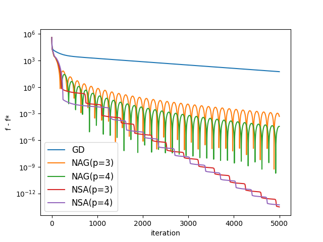
Figure 1: $\min_{\mathbf{x}}\frac{1}{2}\|A\mathbf{x}-\mathbf{b}\|^{2}$

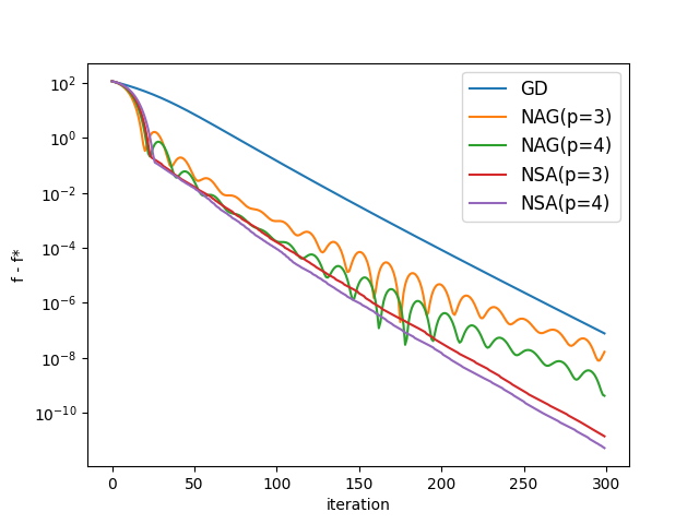
Figure 2: $\min_{\mathbf{x}}\sum_{i=1}^{n}-y_{i}A_{i}^{\top}\mathbf{x}+\log(1+e^{A_{i}^{\top}\mathbf{x}})$

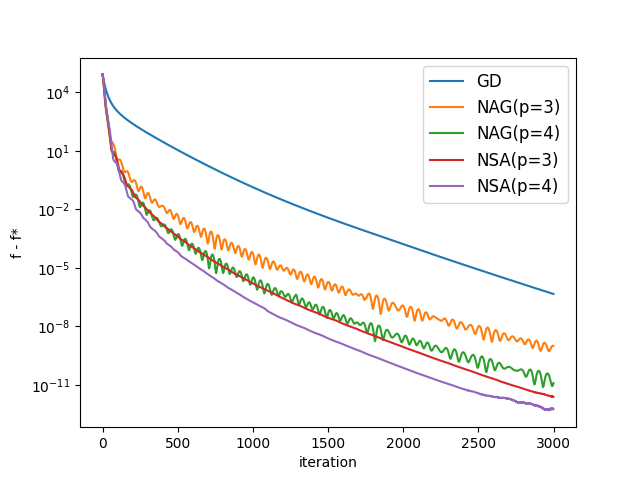
Figure 3: $\min_{\mathbf{x}}\frac{1}{2}\|A\mathbf{x}-\mathbf{b}\|^{2}+\lambda\|x\|_{1}$

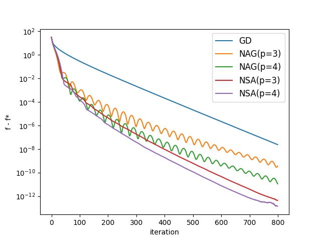
Figure 4: $\min_{\mathbf{x}}\rho\log\left[\sum_{i=1}^{n}\exp(A_{i}^{\top}\mathbf{x}-b_{i})/\rho\right]$

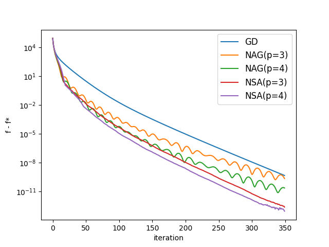
Figure 5: $\min_{\mathbf{x}}\frac{1}{2}\|A\mathbf{x}-\mathbf{b}\|^{2}+\lambda\|\mathbf{x}\|_{2}^{2}$

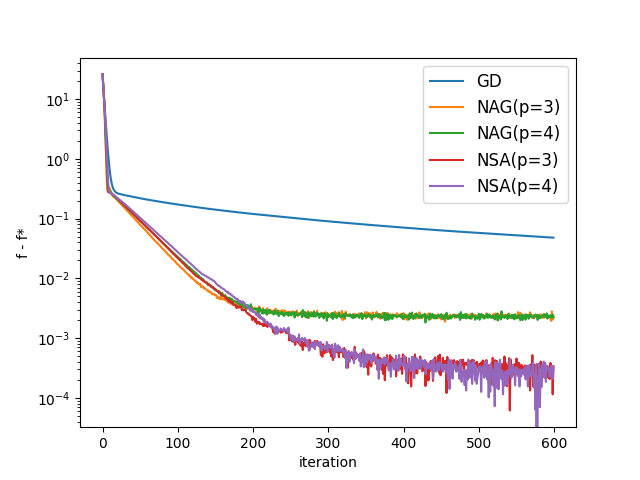
Figure 6: $\min_{\mathbf{x}}\|X_{ob}-A_{ob}\|^{2}+\lambda\|X\|_{*}$

6 Proof of Theorem 3

In this section, we provide a proof of Theorem 3. Together with Theorem 2, this shows that one can construct gradient oracles that satisfies properties (H1) and (H2) using zeroth-order information of the function.

Proof of Theorem 3.

$\mathcal{G}(f,\mathbf{x},\epsilon;\xi)$ satisfies (H2) if the following inequality below is true almost surely

$$\frac{\lvert\langle\nabla f(x)-\mathcal{G}(f,\mathbf{x},\epsilon;\xi),\mathcal{G}(f,\mathbf{x},\epsilon;\xi)\rangle\rvert}{\langle\mathcal{G}(f,\mathbf{x},\epsilon;\xi),\mathcal{G}(f,\mathbf{x},\epsilon;\xi)\rangle}\leq\frac{1}{4}.$$

Using Schwarz inequality, we have

$$\frac{\lvert\langle\nabla f(x)-\mathcal{G}(f,\mathbf{x},\epsilon;\xi),\mathcal{G}(f,\mathbf{x},\epsilon;\xi)\rangle\rvert}{\langle\mathcal{G}(f,\mathbf{x},\epsilon;\xi),\mathcal{G}(f,\mathbf{x},\epsilon;\xi)\rangle}\leq\frac{\lVert\nabla f(x)-\mathcal{G}(f,\mathbf{x},\epsilon;\xi)\rVert}{\lVert\mathcal{G}(f,\mathbf{x},\epsilon;\xi)\rVert}$$ (21)

Furthermore, the triangle inequality gives that

$$\frac{\lVert\nabla f(x)-\mathcal{G}(f,\mathbf{x},\epsilon;\xi)\rVert}{\lVert\mathcal{G}(f,\mathbf{x},\epsilon;\xi)\rVert}\leq\frac{\lVert\nabla f(x)-\mathbb{E}_{\xi}\mathcal{G}(f,\mathbf{x},\epsilon;\xi)\rVert+\lVert\mathbb{E}_{\xi}\mathcal{G}(f,\mathbf{x},\epsilon;\xi)-\mathcal{G}(f,\mathbf{x},\epsilon;\xi)\rVert}{\lVert\mathcal{G}(f,\mathbf{x},\epsilon;\xi)\rVert}$$

Approach 1: Select $\mathcal{G}(f,\mathbf{x},\epsilon;\xi)$ as follows:

$$\mathcal{G}(f,\mathbf{x},\epsilon;\xi)=\frac{1}{2\epsilon}\sum_{k=1}^{n}\left[f(x+\epsilon\mathbf{e_{i}})-f(x-\epsilon\mathbf{e_{i}})\right]\mathbf{e_{i}},\quad\forall\mathbf{x}\in\mathbb{R}^{n}$$

where $\mathbf{e_{i}}$ is the $i$-th unit vector. Then we use the Taylor formula to get

$$\mathcal{G}(f,\mathbf{x},\epsilon;\xi)=\nabla f(x)+o(\epsilon\mathbf{1}),\quad\lVert\mathcal{G}(f,\mathbf{x},\epsilon;\xi)\rVert^{2}=\lVert\nabla f(x)\rVert^{2}+o(\epsilon),$$ (22)

where $\mathbf{1}$ denotes the all-one vector. Therefore, there exists $M_{1}>0,M_{2}>0$,

$$\lVert\mathcal{G}(f,\mathbf{x},\epsilon;\xi)-\nabla f(x)\rVert\leq M_{1}\epsilon,\quad-M_{2}\epsilon\leq\lVert\mathcal{G}(f,\mathbf{x},\epsilon;\xi)\rVert^{2}-\lVert\nabla f(x)\rVert^{2}\leq M_{2}\epsilon$$

We choose $\epsilon$ as $\textbf{min}\{3(4M_{2})^{-1}\lVert\nabla f(x)\rVert^{2},(8M_{1})^{-1}\lVert\nabla f(x)\rVert\}$, then we have

$$\frac{\lVert\nabla f(x)-\mathcal{G}(f,\mathbf{x},\epsilon;\xi)\rVert}{\lVert\mathcal{G}(f,\mathbf{x},\epsilon;\xi)\rVert}\leq\frac{M_{1}\epsilon}{\sqrt{\lVert\nabla f(x)\rVert^{2}-M_{2}\epsilon}}\leq\frac{2M_{1}}{\lVert\nabla f(x)\rVert}\epsilon\leq\frac{1}{4}$$

Therefore, from (21), we conclude that $\mathcal{G}(f,\mathbf{x},\epsilon;\xi)$ above satisfies (H2).
Approach 2: Select $\mathcal{G}(f,\mathbf{x},\epsilon;\xi)$ as follows:

$$\mathcal{G}(f,\mathbf{x},\epsilon;\xi)=\frac{n}{2\epsilon k}\sum_{i=1}^{k}\left[f(\mathbf{x}+\epsilon\mathbf{v}_{i})-f(\mathbf{x}-\epsilon\mathbf{v}_{i})\right]\mathbf{v}_{i},\quad\forall\mathbf{x}\in\mathbb{R}^{n}$$

where $[\mathbf{v}_{1},\mathbf{v}_{2},\cdots,\mathbf{v}_{k}]=\mathbf{V}\in$ $\{\mathbf{X}\in\mathbb{R}^{n\times k}:\mathbf{X}^{\top}\mathbf{X}=\mathbf{I}_{k}\}$ is uniformly sampled.
Select $k=n$, then $[\mathbf{v}_{1},\mathbf{v}_{2},\cdots,\mathbf{v}_{n}]$ is an orthonormal bases for $\mathbb{R}^{n}$, and we have

$$\mathcal{G}(f,\mathbf{x},\epsilon;\xi)=\frac{1}{2\epsilon}\sum_{i=1}^{n}\left[f(\mathbf{x}+\epsilon\mathbf{v}_{i})-f(\mathbf{x}-\epsilon\mathbf{v}_{i})\right]\mathbf{v}_{i},\quad\forall\mathbf{x}\in\mathbb{R}^{n}.$$

Let $v_{i}^{k}$ represents the $k$-th element of $\mathbf{v_{i}}$ . Using the Taylor formula,we have

$$\mathcal{G}(f,\mathbf{x},\epsilon;\xi)=\left(\sum_{i=1}^{n}\sum_{k=1}^{n}\frac{\partial f}{\partial\mathbf{x}_{k}}v_{i}^{k}v_{i}^{p}\right)_{p=1}^{n}+o(\epsilon\mathbf{1})=\left(\sum_{k=1}^{n}\frac{\partial f}{\partial\mathbf{x}_{k}}\left[\sum_{i=1}^{n}v_{i}^{k}v_{i}^{p}\right]\right)_{p=1}^{n}+o(\epsilon\mathbf{1})$$

$[\mathbf{v}_{1},\mathbf{v}_{2},\cdots,\mathbf{v}_{k}]=\mathbf{V}\in$ $\{\mathbf{X}\in\mathbb{R}^{n\times n}:\mathbf{X}^{\top}\mathbf{X}=\mathbf{I}_{n}\}$ So it is obvious that $\mathbf{V}$ is an orthogonal matrix and $\sum_{i=1}^{n}v_{i}^{k}v_{i}^{p}$ is the inner product between the $k$-th column and the $p$-th column. According to the proposition of the orthogonal matrix, we know $\sum_{i=1}^{n}v_{i}^{k}v_{i}^{p}=\delta_{kp}$ , where $\delta_{kp}$ is the Kronecker delta. So we can simplify the formula above as

$$\mathcal{G}(f,\mathbf{x},\epsilon;\xi)=\nabla f(x)+o(\epsilon\mathbf{1})$$

Therefore we get (22). Repeat the process in Approach 1, we can conclude that $\mathcal{G}(f,\mathbf{x},\epsilon;\xi)$ in Approach 2 satisfies (H2). ∎

7 Conclusion

This paper studies the NSA algorithm – a variant of an acceleration method of Nesterov and Spokoiny. NSA converges at rate $o(k^{-2})$ for general smooth convex programs and does not require a proximal oracle. Also, we show that in a continuous-time perspective, the NSA algorithm is governed by a system of first-order ODEs.

Appendix A Standard Conventions for Smooth Convex Optimization

To be self-contained, we briefly review some common conventions for smooth convex optimization. In his book Nesterov, (2018), Nesterov’s discussion on smooth convex optimization focuses on a class of functions $\mathscr{F}$ such that, for any $f\in\mathscr{F}$, $\nabla f(\mathbf{x}^{*})=0$ implies that $\mathbf{x}^{*}$ is a global minimizer of $f$. In addition, $\mathscr{F}$ contains linear functions, and is closed under addition and nonnegative scaling.

Following Nesterov’s convention Nesterov, (2018), we write $f\in\mathscr{F}_{L}^{h,l}(\mathbb{R}^{n})$ ($l\leq h$) if $f\in\mathscr{F}$, and in addition,

• $f$ is convex;

• $f$ is $h$-times continuously differentiable;

• The $l$-th derivative of $f$ is $L$-Lipschitz: There exists $L\in(0,\infty)$ such that

  $$\|\partial^{l}f(\mathbf{x})-\partial^{l}f(\mathbf{x}^{\prime})\|\leq L\|\mathbf{x}-\mathbf{x}^{\prime}\|,\quad\forall\mathbf{x},\mathbf{x}^{\prime}\in\mathbb{R}^{n}.$$

Appendix B Additional Experiments

B.1 Proximal version of NSA

We compare the NSA-prox algorithm (17) with classic gradient descent and the Nesterov Accelerated Gradient (NAG) Nesterov, (1983). In all experiments, we pick the same values of $p$ and $\eta$ for both NSA-prox and NAG. The start point $x_{0}$ is also same for both NSA-prox and NAG. We choose $s=\sqrt{\eta}$.

1. The cost function of least square regression

   $$f(\mathbf{x})=\frac{1}{2}\|A\mathbf{x}-\mathbf{b}\|^{2},$$

   where $A$ is a full-rank $10\times 10$ random matrix sampled from $i.i.d.\>\mathcal{N}(0,1600)$ and $\mathbf{b}$ is a $10\times 1$ vector sampled from $i.i.d\>\mathcal{N}(0,1600)$. We set $\eta=0.00004$ for all algorithms.

1. The cost function of logistics regression

   $$f(\mathbf{x})=\sum_{i=1}^{200}\left[-y_{i}A_{i}^{\top}\mathbf{x}+\log(1+e^{A_{i}^{\top}\mathbf{x}})\right],$$

   where $A=\left(A_{1},...,A_{200}\right)^{\top}$ is a $200\times 5$ random matrix sampled from $i.i.d.$ $\mathcal{N}(0,1)$ and $\mathbf{y}=(y_{1},y_{2},\cdots,y_{200})^{\top}$ is a $200\times 1$ random vector of labels sampled from $i.i.d.\>Ber(1,0.5)$. We set $\eta=0.002$ for all algorithms.

1. The cost function of lasso regression

   $$f(\mathbf{x})=\frac{1}{2}\|A\mathbf{x}-\mathbf{b}\|^{2}+\lambda\|\mathbf{x}\|_{1},$$

   where $A$ is a $400\times 200$ random matrix sampled from $i.i.d.\>\mathcal{N}(0,16)$ and $\lambda=0.05$. Here $\mathbf{b}$ is a $200\times 1$ random vector sampled from $i.i.d.\>\mathcal{N}(0,16)$. We set $\eta=0.0004$ for all algorithms.

1. The log_exp_sum function

   $$f(\mathbf{x})=\rho\log\left[\sum_{i=1}^{n}e^{(A_{i}^{\top}\mathbf{x}-b_{i})/\rho}\right],$$

   where $A=\left(A_{1},...A_{200}\right)^{\top}$ is a $200\times 50$ random matrix sampled from $i.i.d.$ $\mathcal{N}(0,40)$ and $\mathbf{b}=(b_{1},b_{2},\cdots,b_{200})^{\top}$ is a $200\times 1$ random vector sampled from $i.i.d.$ $\mathcal{N}(0,800)$. Let $n=200$, $\rho=20$. We set $\eta=0.5$ for all algorithms.

1. The cost function of ridge regression

   $$f(\mathbf{x})=\frac{1}{2}\|A\mathbf{x}-\mathbf{b}\|^{2}+\lambda\|\mathbf{x}\|_{2}^{2},$$

   where $A$ is a $400\times 200$ random matrix sampled from $i.i.d\>\mathcal{N}(0,16)$, $\lambda=0.05$. Here $\mathbf{b}$ is a $200\times 1$ random vector sampled from $i.i.d.\>\mathcal{N}(0,16)$. We set $\eta=0.0005$ for all algorithms.

1. The cost function of matrix completion

   $$f(X)=\|X_{ob}-A_{ob}\|^{2}+\lambda\|X\|_{*},$$

   where $A_{ob}$ includes the available elements in matrix $A$ and only 20% of the elements in $A$ can be observed. The position of these elements is randomly chosen and the original matrix $A$ is a rank-7 $50\times 40$ matrix with the eigenvalues—$\left[1,2,3,4,5,6,7\right]$. To generate $A$, we generate $U,S$ and $V$ where $S=diag\{1,2,\cdots,7\}$ and $U,V^{\top}$ are rank-7 $50\times 7$ matrices generated from $i.i.d\>Uniform(0,1)$. Then we calculate $A$ by $A=USV$ and set $\lambda=0.05$. We set $\eta=0.1$ for all algorithms.

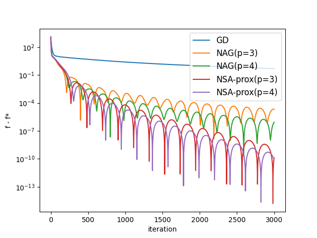
Figure 7: $\min_{\mathbf{x}}\frac{1}{2}\|A\mathbf{x}-\mathbf{b}\|^{2}$

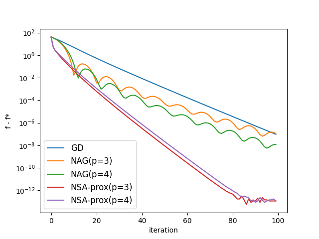
Figure 8: $\min_{\mathbf{x}}\sum_{i=1}^{n}-y_{i}A_{i}^{\top}\mathbf{x}+\log(1+e^{A_{i}^{\top}\mathbf{x}})$

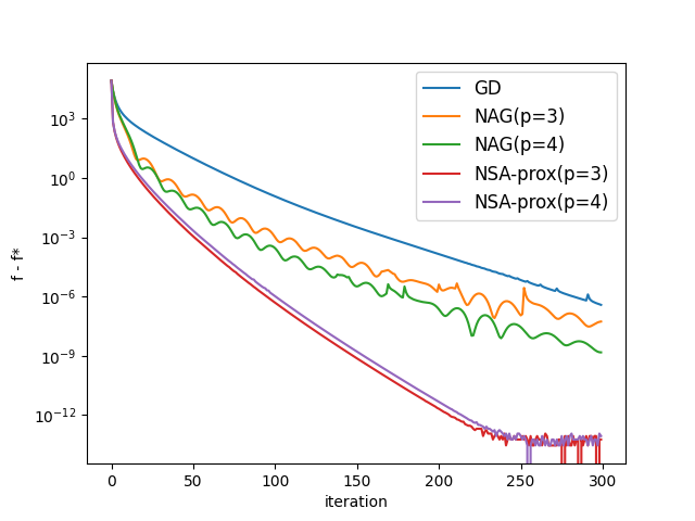
Figure 9: $\min_{\mathbf{x}}\frac{1}{2}\|A\mathbf{x}-\mathbf{b}\|^{2}+\lambda\|\mathbf{x}\|_{1}$

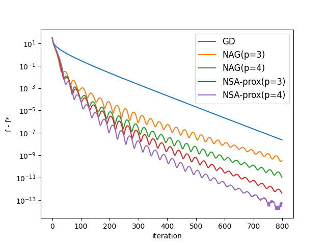
Figure 10: $\min_{\mathbf{x}}\rho\log\left[\sum_{i=1}^{n}\exp(A_{i}^{\top}\mathbf{x}-b_{i})/\rho\right]$

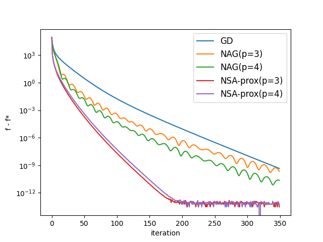
Figure 11: $\min_{\mathbf{x}}\frac{1}{2}\|A\mathbf{x}-\mathbf{b}\|^{2}+\lambda\|\mathbf{x}\|_{2}^{2}$

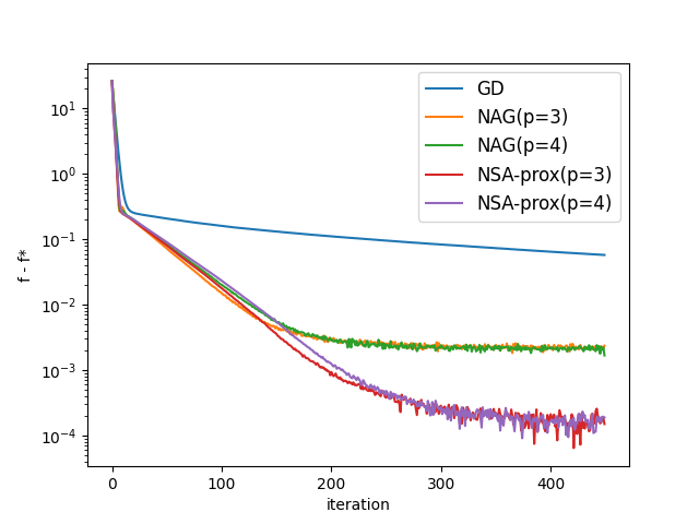
Figure 12: $\min_{X}\|X_{ob}-A_{ob}\|^{2}+\lambda\|X\|_{*}$

B.2 Zeroth-order version of NSA

We compare the NSA-zero algorithm (2) with classic gradient descent and the Nesterov Accelerated Gradient (NAG) Nesterov, (1983). In all experiments, we pick the same values of $p$ and $\eta$ for both NSA-zero and NAG. The start point $\mathbf{x}_{0}$ is also same for both NSA-zero and NAG. We choose the gradient estimation $\mathcal{G}$ as

$$\mathbf{g}_{t}(\mathbf{x})=\frac{1}{2\epsilon_{t}}\sum_{i=1}^{n}\left[f(\mathbf{x}+\epsilon_{t}\mathbf{v}_{i})-f(\mathbf{x}-\epsilon_{t}\mathbf{v}_{i})\right]\cdot\mathbf{v}_{i}.$$

1. The cost function of least square regression

   $$f(\mathbf{x})=\frac{1}{2}\|A\mathbf{x}-\mathbf{b}\|^{2},$$

   where $A$ is a full-rank $10\times 10$ random matrix sampled from $i.i.d.\>\mathcal{N}(0,1600)$ and $\mathbf{b}$ is a $10\times 1$ vector sampled from $i.i.d\>\mathcal{N}(0,1600)$. Let $h(t)=\min\{t,50\}.$ We set $\eta=0.00005$ for all algorithms and $\epsilon_{t}=2^{-h(t)}$ for NSA-zero.

1. The cost function of logistics regression

   $$f(\mathbf{x})=\sum_{i=1}^{200}\left[-y_{i}A_{i}^{\top}\mathbf{x}+\log(1+e^{A_{i}^{\top}\mathbf{x}})\right],$$

   where $A=\left(A_{1},...,A_{200}\right)^{\top}$ is a $200\times 5$ random matrix sampled from $i.i.d.$ $\mathcal{N}(0,1)$ and $\mathbf{y}=(y_{1},y_{2},\cdots,y_{200})^{\top}$ is a $200\times 1$ random vector of labels sampled from $i.i.d.\>Ber(1,0.5)$. Let $h(t)=\min\{t,50\}.$ We set $\eta=0.002$ for all algorithms and $\epsilon_{t}=2^{-h(t)}$ for NSA-zero.

1. The cost function of lasso regression

   $$f(\mathbf{x})=\frac{1}{2}\|A\mathbf{x}-\mathbf{b}\|^{2}+\lambda\|\mathbf{x}\|_{1},$$

   where $A$ is a $50\times 20$ random matrix sampled from $i.i.d.\>\mathcal{N}(0,16)$ and $\lambda=0.05$. Here $\mathbf{b}$ is a $50\times 1$ random vector sampled from $i.i.d.\>\mathcal{N}(0,16)$. Let $h(t)=\min\{t,200\}.$ We set $\eta=0.00005$ for all algorithms and $\epsilon_{t}=2^{-0.1h(t)}$ for NSA-zero.

1. The log_exp_sum function

   $$f(\mathbf{x})=\rho\log\left[\sum_{i=1}^{n}e^{(A_{i}^{\top}\mathbf{x}-b_{i})/\rho}\right],$$

   where $A=\left(A_{1},...A_{100}\right)^{\top}$ is a $100\times 20$ random matrix sampled from $i.i.d.$ $\mathcal{N}(0,40)$ and $\mathbf{b}=\left(b_{1},...b_{100}\right)^{\top}$ is a $100\times 1$ random vector sampled from $i.i.d.$ $\mathcal{N}(0,800)$. Let $n=100,\rho=10,h(t)=\min\{t,200\}.$ We set $\eta=0.02$ for all algorithms and $\epsilon_{t}=2^{-0.1h(t)}$ for NSA-zero.

1. The cost function of ridge regression

   $$f(\mathbf{x})=\frac{1}{2}\|A\mathbf{x}-\mathbf{b}\|^{2}+\lambda\|\mathbf{x}\|_{2}^{2},$$

   where $A$ is a $50\times 20$ random matrix sampled from $i.i.d\>\mathcal{N}(0,16)$, $\lambda=0.05$. Here $\mathbf{b}$ is a $20\times 1$ random vector sampled from $i.i.d.\>\mathcal{N}(0,16)$. Let $h(t)=\min\{t,200\}.$ We set $\eta=0.00005$ for all algorithms and $\epsilon_{t}=2^{-0.1h(t)}$ for NSA-zero.

1. The cost function of matrix completion

   $$f(X)=\|X_{ob}-A_{ob}\|^{2}+\lambda\|X\|_{*},$$

   where $A_{ob}$ includes the available elements in matrix $A$ and only 20% of the elements in $A$ can be observed. The position of these elements is randomly chosen and the original matrix $A$ is a rank-7 $50\times 40$ matrix with the eigenvalues—$\left[1,2,3,4,5,6,7\right]$. To generate $A$, we generate $U,S$ and $V$ where $S=diag\{1,2,\cdots,7\}$ and $U,V^{\top}$ are rank-7 $50\times 7$ matrices generated from $i.i.d\>Uniform(0,1)$. Then we calculate $A$ by $A=USV$. Let $\lambda=0.05$, $h(t)=\min\{t,200\}.$ We set $\eta=0.1$ for all algorithms and $\epsilon_{t}=2^{-0.1h(t)}$ for NSA-zero.

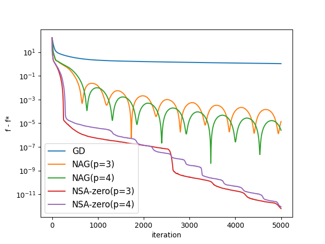
Figure 13: $\min_{\mathbf{x}}\frac{1}{2}\|A\mathbf{x}-\mathbf{b}\|^{2}$

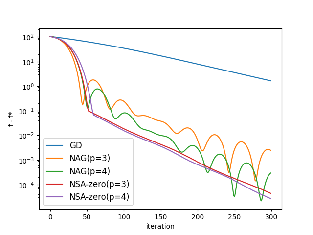
Figure 14: $\min_{\mathbf{x}}\sum_{i=1}^{n}-y_{i}A_{i}^{\top}\mathbf{x}+\log(1+e^{A_{i}^{\top}\mathbf{x}})$

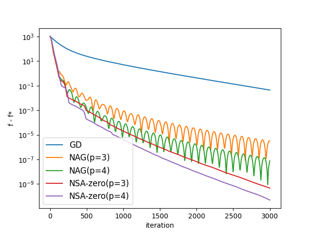
Figure 15: $\min_{\mathbf{x}}\frac{1}{2}\|A\mathbf{x}-\mathbf{b}\|^{2}+\lambda\|\mathbf{x}\|_{1}$

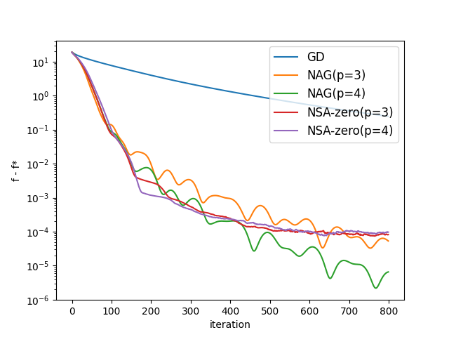
Figure 16: $\min_{\mathbf{x}}\rho\log\left[\sum_{i=1}^{n}\exp(A_{i}^{\top}\mathbf{x}-b_{i})/\rho\right]$

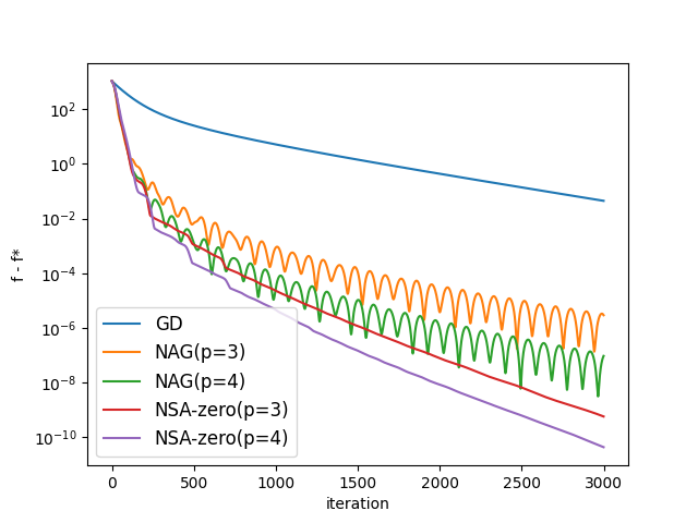
Figure 17: $\min_{\mathbf{x}}\frac{1}{2}\|A\mathbf{x}-\mathbf{b}\|^{2}+\lambda\|\mathbf{x}\|_{2}^{2}$

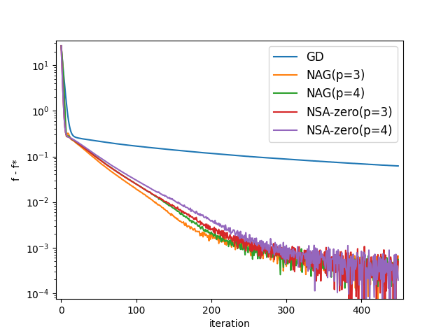
Figure 18: $\min_{X}\|X_{ob}-A_{ob}\|^{2}+\lambda\|X\|_{*}$

References

- (1) Allen-Zhu, Z. and Orecchia, L. (2014a). Linear coupling: An ultimate unification of gradient and mirror descent. arXiv preprint arXiv:1407.1537.
- (2) Allen-Zhu, Z. and Orecchia, L. (2014b). Linear coupling: An ultimate unification of gradient and mirror descent. Mathematics.
- Alvarez and Attouch, (2001) Alvarez, F. and Attouch, H. (2001). An inertial proximal method for maximal monotone operators via discretization of a nonlinear oscillator with damping. Set-Valued Analysis, 9:3–11.
- Alvarez et al., (2002) Alvarez, F., Attouch, H., Bolte, J., and Redont, P. (2002). A second-order gradient-like dissipative dynamical system with hessian-driven damping.: Application to optimization and mechanics. Journal de Mathématiques Pures et Appliquées, 81(8):747–779.
- Arnold, (1989) Arnold, V. (1989). Mathematical methods of classical mechanics, volume 60. Springer Science & Business Media.
- Attouch et al., (2022) Attouch, H., Chbani, Z., Fadili, J., and Riahi, H. (2022). First-order optimization algorithms via inertial systems with hessian driven damping. Mathematical Programming, pages 1–43.
- Attouch et al., (2018) Attouch, H., Chbani, Z., Peypouquet, J., and Redont, P. (2018). Fast convergence of inertial dynamics and algorithms with asymptotic vanishing viscosity. Mathematical Programming, 168:123–175.