Robust Dynamic Operating Envelopes via Superellipsoid-based Convex Optimisation in Unbalanced Distribution Networks

Abstract

Dynamic operating envelopes (DOEs) have been introduced to integrate distributed energy resources (DER) in distribution networks via real-time management of network capacity limits. Recent research demonstrates that uncertainties in DOE calculations should be carefully considered to ensure network integrity while minimising curtailment of consumer DERs. This letter proposes a novel approach to calculating DOEs that is robust against uncertainties in the utilisation of allocated capacity limits and demonstrates that the reported solution can attain close to global optimality performance compared with existing approaches.

I Introduction

Dynamic operating envelopes (DOEs) specify the operational capacity range for consumer DERs that is permissible at their connection point and appear as a key enabler of emerging flexible power system architectures and have gained growing interest within industry and academia as an instrument to efficiently manage DER export/import limits [1, 2]. With substantial advances being made in developing approaches to calculating DOEs, recent publications revealed that uncertainties arising from parameter or forecast accuracy and true utilisation of DOEs need to be carefully catered for to make the calculated DOEs more robust [3, 4, 5].

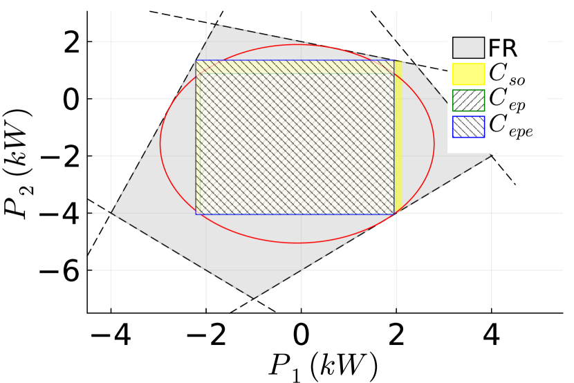
(a) RDOE concept.

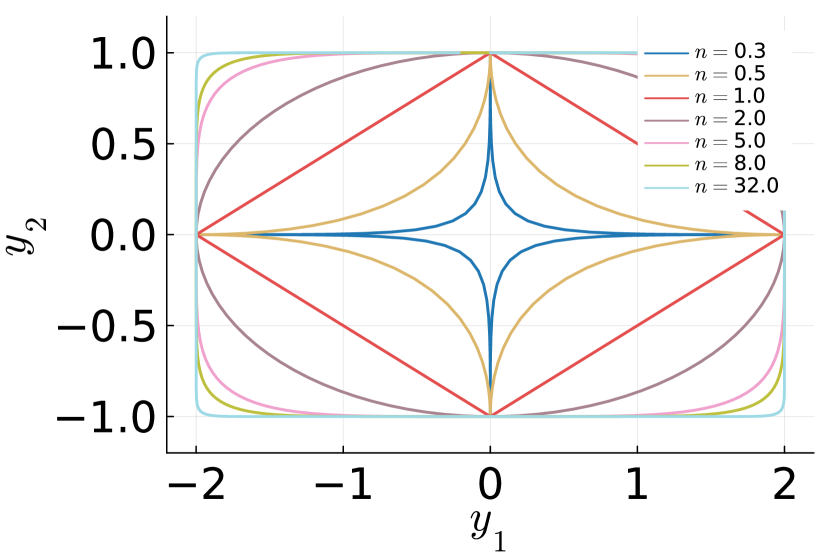
(b) Superellipsoid concept.

Figure 1: (a) Conceptual example in calculating RDOEs via three steps; (b) Superellipsoid with $u_{c}=[0,0]^{T}$ and $L=[2,0;0,1]$.

In [3], a linear unbalanced three-phase optimal power flow (UTOPF)-based approach was proposed to calculate the robust DOEs (RDOEs), which can explicitly hedge against uncertainties in active customers’ utilisation of their allocated capacities. The RDOE concept can be explained by the feasible region (FR) for DERs [6], as shown in Fig.1(a). For the two active customers, even if the allocated DOEs are $(-4\leavevmode\nobreak\ \text{kW},\leavevmode\nobreak\ -4\leavevmode\nobreak\ \text{kW})$, operational violations can still occur, noting that any operational point $(P_{1},P_{2})$ with $P_{1}=-4\leavevmode\nobreak\ \text{kW}$ and $P_{2}>-4\leavevmode\nobreak\ \text{kW}$ will be out of the FR. To address the robustness issue, a three-step approach capable of considering the operational statuses of active customers and optimising controllable reactive powers was proposed in [3]. As shown in Fig.1(a), the approach includes: 1) seeking the maximum hyperrectangle ($\mathcal{C}_{ep}$), measured as its volume, within the FR as a strategy to decouple the interdependence of DOEs for all active customers via the maximum inscribed hyperellipsoid (red curve), which also reports optimal dispatched reactive powers; 2) With fixed optimal reactive dispatch, removing redundant constraints from the updated FR; and 3) Expanding the $\mathcal{C}_{ep}$ based on Motzkin Transposition Theorem (MTT), leading to $\mathcal{C}_{epe}$ and the RDOEs.

However, compared with the stochastic optimisation (SO)-based approach ($\mathcal{C}_{so}$ in Fig.1(a)), sub-optimality in the three-step approach is inevitable due to optimising reactive powers in the first step only and the non-convex formulation in the final step. To further improve the optimality of the solution, this letter proposes a novel approach that can report a solution close enough to global optimality. The contributions of this letter are: 1) A convex formulation is proposed based on a superellipsoid (instead of a hyperellipsoid in the first step in the three-step approach) to seek the maximum hyperrectangle within the FR in one step, thus bypassing the remaining steps in the original procedure; 2) An approach is proposed to select the superellipsoid “squareness” parameter to achieve a pre-specified level or near-optimality; 3) Compared with the previous three-step approach, it is shown that a near-optimal solution, sufficiently close to global optimality for practical purposes, can be guaranteed at the expense of a manageable increase in computation time.

II RDOE via Superellipsoid-based Convex Optimisation

II-A FR and the definition of superellipsoid

As discussed in [3], based on a UTOPF model with appropriate linearisation techniques, FR for active powers of all active customers can be compactly expressed as the following polyhedron.

$$\small\mathcal{F}(q)=\left\{p\left|\begin{matrix}Ap+Bq+Cv=d\\ Ev\leq f\\ \end{matrix}\right.\right\}=\left\{p\left|\begin{matrix}\bar{E}Ap\leq\\ f+\bar{E}(d-Bq)\\ \end{matrix}\right.\right\}$$ (1)

where $p$ and $q$ are variables corresponding to DOEs and reactive powers to be optimised, respectively; $v$ is a vector consisting of variables related to nodal voltages; $A,B,C,d,E$ and $f$ are constant parameters with appropriate dimensions and $\bar{E}=-EC^{-1}$.

The definition of the superellipsoid will be presented next, followed by the problem formulation in the next section.

A $n$-dimension superellipsoid, with the centre being $u_{c}$ and lengths of all axes defined by a positive definite diagonal matrix $L$, can be expressed as $\mathcal{P}=\{p|p=Lw+u_{c},||w||_{n}^{n}\leq 1\}$ with $w_{i}$ being the $i^{th}$ element of $w$. Fig.1(b) presents the boundary curves of $\mathcal{P}$ under various $n$, which shows that $\mathcal{P}$ is convex when $n\geq 1$ and becomes closer to the rectangle along with increasing value of $n$. Specially, when $n=2^{K}$ with $K$ being a positive integer, $\mathcal{P}$ can be expressed as $\mathcal{P}=\{p|p=Lw+u_{c},\leavevmode\nobreak\ w\in\mathcal{E}_{h}\}$, where $\mathcal{E}_{h}=\left\{y_{1}|\begin{array}[]{cc}y_{k,i}^{2}\leq y_{k+1,i}\leavevmode\nobreak\ \forall i,\forall k\leq K-1;||y_{K}||_{2}\leq 1\end{array}\right\}$ and $y_{k}$ is an intermediate vector variable with $y_{k,i}$ being its $i^{th}$ element. Moreover, $\mathcal{E}_{h}$ contains $mK+1$ quadratic constraints, where $m$ is the cardinality of $y_{k}$.

II-B Mathematical formulation

Noting that maximising the inscribed hyperrectangle regarding its volume, say $V_{h}$, is equivalent to $\max_{L}\det(L)$ noting that

1. $V_{h}=2^{v}\prod\nolimits|L_{ii}w_{i}|=2^{v}\det(L)\prod\nolimits_{i}w_{i}$ with $v$ being the total number of active customers;

2. $w_{i}^{*}=\arg\max\nolimits_{w:\norm{w}_{n}^{n}=1}{2^{v}\det(L)\sum\nolimits{\log(w_{i})}}=v^{-1/n}$, the latter of which can be proved by applying the KKT condition when fixing $L$, leading to $V_{h}=(2v^{-1/n})^{v}\det(L)$.

Then, $V_{h}$ can be maximised as follows by considering customers’ operational statuses after replacing $n$ by $2^{K}$.

$$\max_{\underline{q}\leq q\leq\bar{q},L,u_{c}}{\log(\det(L))}-\varepsilon_{md}\sum\nolimits_{i}\delta_{i}$$ (2a)

$$s.t.\leavevmode\nobreak\ \leavevmode\nobreak\ \bar{E}ALy_{1}+\bar{E}Au_{c}\leq f+\bar{E}(d-Bq)\leavevmode\nobreak\ \leavevmode\nobreak\ \forall y_{1}\in\mathcal{E}_{h}$$ (2b)

$$-\delta_{i}\leq u_{c}(i)-\lambda_{i}L_{ii}v^{-1/2^{K}}\leq\delta_{i}\leavevmode\nobreak\ \leavevmode\nobreak\ \forall i$$ (2c)

where $\varepsilon_{md}$ is a penalty factor; $\delta_{i}$ is a non-negative slack variable for customer $i$; $u_{c}(i)$ is the $i^{th}$ element of vector $u_{c}$; $\lambda_{i}$ is a binary number to indicate the operational status of customer $i$ with $\lambda_{i}=1/-1/0$ indicating import/ export/unknown (could be import or export), and $\underline{q}$ and $\bar{q}$ are the lower and upper limits for $q$, respectively.

Obviously, as shown in (2c), the lower and upper capacity limits for customer $i$ are respectively $u_{c}(i)-L_{ii}v^{-1/2^{K}}$ and $u_{c}(i)+L_{ii}v^{-1/2^{K}}$, with $u_{c}(i)$ and $L_{ii}$ to be optimised.

Constraint (2c), together with (2a), ensure the export/import limit is as close to 0 kW as possible when the customer is importing/exporting power so it can freely vary its power between 0 kW and the allocated capacity limit. For example, if customer $i$ is exporting power, $|u_{c}(i)+{L_{ii}}v^{-1/2^{K}}|$, as its import limit, will be penalised in the objective function. Further, if a customer’s operational status is unknown, $\sum\nolimits_{i}|u_{c}(i)|$ will be penalised in the objective function, leading to a DOE allocation where the import and export limits in their absolute values are as close to each other as possible.

To derive the robust counterpart (RC) of (2) with respect to uncertain $y_{1}\in\mathcal{E}_{h}$ in (2b), the dual formulation of (3), which is a generalised formulation for seeking the maximum value for the first term on the left-hand side of (2b), needs to be derived.

$$\max\nolimits_{y_{1},\cdots,y_{K}}x^{T}y_{1}$$ (3a)

$$s.t.\leavevmode\nobreak\ \leavevmode\nobreak\ y_{k,i}^{2}\leq y_{k+1,i}\leavevmode\nobreak\ \leavevmode\nobreak\ \forall k\leq K-1,\forall i\leavevmode\nobreak\ \leavevmode\nobreak\ (\alpha_{k,i})$$ (3b)

$$||y_{K}||_{2}\leq 1\leavevmode\nobreak\ \leavevmode\nobreak\ (\alpha_{K})$$ (3c)

where $x$ is a known vector representing a single row of $\bar{E}AL$, and $\alpha_{k,i}$ and $\alpha_{K}$ are Lagrangian multipliers.

Noting that the Lagrangian function for (3) is

$$W(\alpha_{k,i},\alpha_{K},y_{k})=-\sum_{2\leq k\leq K-1}\sum_{i}\left[\alpha_{k,i}y_{k,i}^{2}-\alpha_{k-1,i}y_{k,i}\right]$$

$$-\sum_{i}\left[\alpha_{1,i}y_{1,i}^{2}-x_{i}y_{1,i}\right]-\alpha_{K}(||y_{K}||_{2}-1)+\alpha_{K-1}^{T}y_{K}$$ (4a)

$$\leq\sum_{i}\frac{x_{i}^{2}}{4\alpha_{1,i}}+\sum_{2\leq k\leq K-1}\sum_{i}\frac{\alpha_{k-1,i}^{2}}{4\alpha_{k,i}}-\alpha_{K}(||y_{K}||_{2}-1)+\alpha_{K-1}^{T}y_{K}$$ (4b)

Then $\min_{\alpha_{k,i},\alpha_{K}}\max_{y_{k}}W(\alpha_{k,i},\alpha_{K},y_{k})$, which is the equivalent problem of (3), can be further formulated as

$$\min_{\alpha_{k,i},\alpha_{K}}\alpha_{K}+\sum_{i}{x_{i}^{2}}/{4\alpha_{1,i}}+\sum_{2\leq k\leq K-1}\sum_{i}{\alpha_{k-1,i}^{2}}/{4\alpha_{k,i}}$$ (5a)

$$s.t.\leavevmode\nobreak\ \leavevmode\nobreak\ ||\alpha_{K-1}||_{2}\leq\alpha_{K}$$ (5b)

By introducing intermediate variables $t_{m,k,i}$, replacing $x$ by $[\bar{E}AL]_{m}^{T}$ and removing min operator in (5a), (2) can be reformulated as

$$\max_{\underline{q}\leq q\leq\bar{q},L,u_{c}}{\log(\det(L))}-\varepsilon_{md}\sum\nolimits_{i}\delta_{i}$$ (6a)

$$s.t.\leavevmode\nobreak\ \alpha_{m,K}+\sum\nolimits_{k\leq K-1}\sum\nolimits_{i}t_{m,k,i}+[\bar{E}Au_{c}]_{m}$$

$$\leq[f+\bar{E}d]_{m}-[\bar{E}Bq)]_{m}\leavevmode\nobreak\ \leavevmode\nobreak\ \forall m$$ (6b)

$$([\bar{E}AL]_{m,i})^{2}\leq 4\alpha_{m,1,i}t_{m,1,i}\leavevmode\nobreak\ \forall m,\forall i$$ (6c)

$$\alpha_{m,k-1,i}^{2}\leq 4\alpha_{m,k,i}t_{m,k,i}\leavevmode\nobreak\ \forall m,\forall k\in\{2,\cdots,K-1\},\forall i$$ (6d)

$$||\alpha_{m,K-1}||_{2}\leq\alpha_{m,K}\leavevmode\nobreak\ \forall m\leavevmode\nobreak\ \text{and}\leavevmode\nobreak\ \eqref{opt_02_rc}$$ (6e)

where $[\cdot]_{m}$ represents the $m^{th}$ row of a matrix or the $m^{th}$ element of a vector, and $[\cdot]_{m,i}$ represents the $(m,i)^{th}$ element of a matrix.

Several remarks are given below.

1. Since $\log(\det(L))$ is concave in $L$ and $x^{2}\leq 4yz$ is equivalent to $||x;\leavevmode\nobreak\ y-z||_{2}\leq y+z$, which is a second-order cone (SOC) constraint, (6) is a convex optimisation problem.

2. For FR with $M$ inequalities and $v$ active customers, $M$ linear and $v\times M(K-1)+M$ quadratic constraints exist in (6), implying higher computational burden with larger $K$.

3. As the total DOE, defined as the absolute sum of all calculated capacity limits, is $S_{h}=2\sum\nolimits_{i}L_{ii}v^{-1/2^{K}}$ according to (2c), the maximum total DOE achievable is $\bar{S}_{h}=2\sum\nolimits_{i}L_{ii}$ when $K\rightarrow\infty$. With a given positive $\theta$ to make sure $1-S_{h}/\bar{S}_{h}\leq\theta$, there is $K\geq(\log(\log v)-\log(-\log{(1-\theta)}))/\log{2}$. The value of $1-S_{h}/\bar{S}_{h}$ under various $K$ when $\theta=0.01$ is presented in Fig.2, showing that setting $K$ as 10 can achieve acceptable accuracy with more than 500 active customers.

   

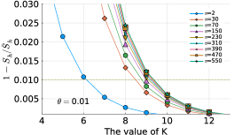
   Figure 2: The value of $1-S_{h}/\bar{S}_{h}$ with varying $K$.

4. To further improve the computational efficiency, by introducing the intermediate variable $\gamma_{ii}$, the logarithmic term in (6a) can be replaced by $\sum\nolimits_{i}\gamma_{ii}$ and an extra constraint $\gamma_{ii}\leq({L_{ii}-\bar{L}_{ii}^{k}})/{\bar{L}_{ii}^{k}}+\log\bar{L}_{ii}^{k}\leavevmode\nobreak\ (\forall k)$ with $\bar{L}_{ii}^{k}$ being the $k^{th}$ predefined point for the $i^{th}$ logarithmic term. Generally, a larger number of predefined points, although leading to higher accuracy, results in higher computational complexity.

5. The problem (6) for both small-scale networks (the TwbAusNetworks in Section III) and networks of larger scales (the AusNetwork and SynNetwork in Section III) are solved by Mosek (version 10.0.40) on a desktop machine with Intel(R) Core(TM) i9-9900 CPU and 32 GB RAM after linearising (6a). For the three-step approach, Ipopt is employed for small-scale networks while Mosek and Knitro (trial version 13.2.0) are employed for others due to computational limitation of Ipopt, as discussed in [3]. Moreover, removing redundant constraints in the second step of the three-step approach is via Xpress (version 41.01.0).

III Case Study

Three distribution networks are considered: a 2-bus illustrative network (TwbNetwork), a 33-bus representative Australian network (AusNetwork) and a 132-bus synthetic network constructed by extending the AusNetwork (SynNetwork); see [3] for more details. For the 2-bus TwbNetwork, an ideal balanced voltage source with the voltage magnitude being $1.0\leavevmode\nobreak\ p.u.$ is connected to bus 1 and three customers (customers 1, 2 and 3) are connected to phase $b,a$ and $c$ of bus 2, respectively, where customer 2 is with fixed active/reactive power while DOEs are to be calculated for customers 1 and 3 with their reactive powers being controllable. The impedance of the three-phase line connecting bus 1 and bus 2 can be found in [3]. The AusNetwork/SynNetwork have 33/132 buses and 87/348 customers, of which 30/116 are active customers with controllable reactive powers. For the remaining passive customers, their active and reactive powers are fixed. The default limits on active and reactive powers for all studied networks are set as [-7 kW, 7 kW] and [-3 kvar, 3 kvar], respectively. The topology of the AusNetwork is presented in Fig.3, and the SynNetwork is generated by replicating the AusNetwork itself at buses “40”, “55” and “65”. More details of the data, including network parameters, customers’ locations and load profiles for passive customers, can be found in [3] and [7] (Network J) and are omitted here for simplicity.

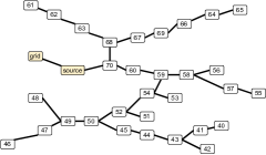
Figure 3: Topology of the AusNetwork (Information for customers’ locations is available in [7] (Network J). Especially, customers 30, 21, 16, 29, 2, 18, 22, 19 and 17, which are constrained in Fig.5, are connected to buses 64, 40, 45, 65, 65, 41, 40, 46 and 42, respectively).

Simulation results for the TwbNetwork when customers 1 and 3 are importing powers are presented in Fig.1 and Table I. The deterministic approach (denoted as “Dmtd”) overestimates the DOEs compared with the globally optimal RDOEs (indicated by “SO”). For the three-step approach (indicated by “3step”), although RDOEs are ameliorated by the third step, noting the difference between the initial RDOEs (denoted by “3step_fnl”) and the final RDOEs (indicated by “3step_ini”), it is still sub-optimal. By contrast, the superellipsoid-based approach (indicated by “sESD”) reports almost the same result as the SO-based approach when $\theta=0.01$ or $K=7$, demonstrating the efficiency of the proposed approach.

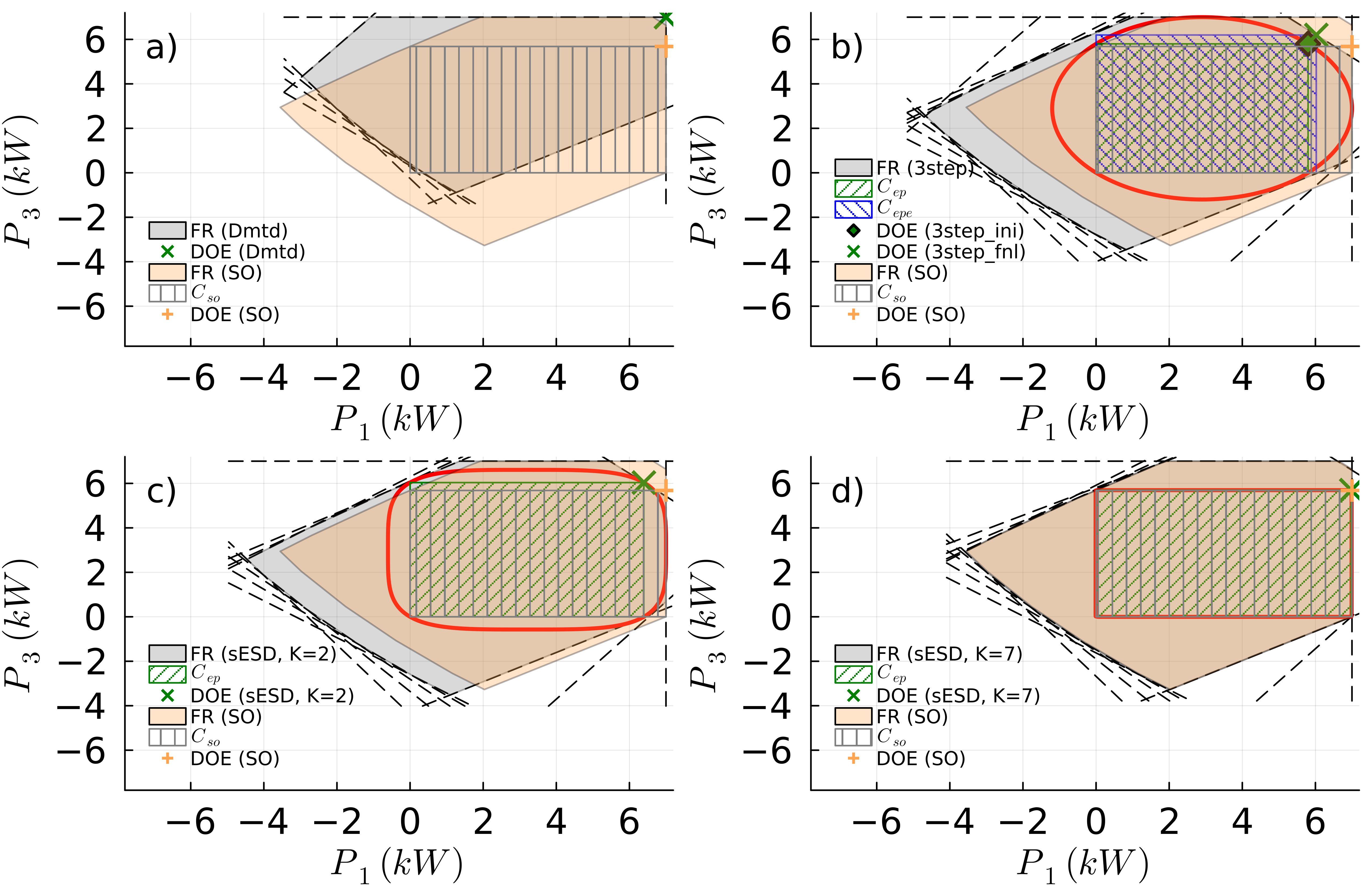
Figure 4: FRs and RDOEs compared with SO-based method under various approaches for TwbNetwork (boundaries for identified hyperellipsoid and superellipsoid are marked in red), where a): Dmtd; b): Three-step; c): sESD($K=2$); d): sESD($K=7$).

Table I: Total DOE calculated in kW under various approaches ($K^{*}$ set as 7/9/9 for TwbNetwork/AusNetwork/SynNetwork and the computational time in seconds are given under the calculated DOE in bracket).

Network/Approach	Dmtd	3step	sESD ($K=2$)	sESD ($K=K^{*}$)	SO
TwbNetwork	14.0 (0.01 s)	12.2 (0.10 s)	12.4 (0.29 s)	12.7 (0.94 s)	12.7 (0.03 s)
AusNetwork	210.0 (0.12 s)	149.5 (28.46 s)	116.3 (21.47 s)	165.8 (102.14 s)	—
SynNetwork	812.0 (0.32 s)	230.8 (303.39 s)	175.7 (231.53 s)	269.0 (1504.01 s)	—

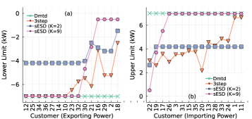
Figure 5: DOEs calculated by various approaches for the AusNetwork, where customers in sub-figure (a)/(b) are exporting/importing powers and their upper/lower limits are 0 kW.

For the AusNetwork, the calculated DOEs are presented in Fig.4 and Table I, where the deterministic approach again reports over-estimated results. Compared with the three-step approach, the total DOE calculated by the superellipsoid approach increases by 10.89% to 165.8 kW when $K=9$ with, however, increased computational time, where the logarithmic terms are linearised with 15 predefined points. It is noteworthy that customers with locations at or near the network’s endpoints have smaller allocated capacity limits. This is because voltage levels at endpoints are either higher or lower than those at internal locations, making customers at or close to them more likely to be constrained.

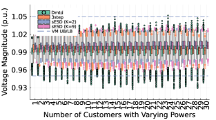
Figure 6: DOE assessment based on exact UTPF for the AusNetwork.

Further assessment of the calculated DOEs by running exact UTPFs with random load profiles on the AusNetwork is presented in Fig.6, which clearly shows that the deterministic approach leads to significant voltage violations. In contrast, other approaches can guarantee operational security.

The simulation results for the SynNetwork are presented in Table I, which again demonstrates that the deterministic approach overestimates the DOEs. In contrast, the superellipsoid-based approach increases the total DOE by 16.55% compared with the three-step approach with $K=9$. Although the computational time increases to more than 1500 seconds, it is still acceptable when DOEs are calculated day-ahead, hourly or every several hours in intra-day operation. It is noteworthy that, since all extreme points of the hyperrectangle need to be enumerated in the SO approach, the constraints in the formulated problem would be more than $2^{30}>$1 billion and $2^{116}$ for the AusNetwork and SynNetwork, respectively, which leads to computational intractability. Thus, the SO approach is not tested for the two networks.

IV Conclusions

This letter proposes a superellipsoid-based approach to calculate RDOEs that can report a solution arbitrarily close to the global optimal via convex optimisation, in contrast to existing sub-optimal approaches. Increased computational time can be managed by selecting a proper parameter in formulating the superellipsoid while achieving the required accuracy, and in practice via a machine with higher computing power or a suitable time resolution, for example, every day, hourly or every several hours, to update the RDOEs if the computing power is limited.

References

- [1] “Dynamic Operating Envelopes working group outcomes report,” Distributed Energy Integration Program (DEIP), Melbourne, Australia, Tech. Rep. March, 2022. [Online]. Available: https://arena.gov.au/assets/2022/03/dynamic-operating-envelope-working-group-outcomes-report.pdf
- [2] M. Z. Liu, L. N. Ochoa, S. Riaz, P. Mancarella, T. Ting, J. San, and J. Theunissen, “Grid and Market Services From the Edge: Using Operating Envelopes to Unlock Network-Aware Bottom-Up Flexibility,” IEEE Power and Energy Magazine, vol. 19, no. 4, pp. 52–62, 2021.
- [3] B. Liu and J. H. Braslavsky, “Robust dynamic operating envelopes for DER integration in unbalanced distribution networks,” IEEE Trans. Power Syst., doi: 10.1109/TPWRS.2023.3308104, pp. 1–15, 2023.
- [4] ——, “Sensitivity and Robustness Issues of Operating Envelopes in Unbalanced Distribution Networks,” IEEE Access, vol. 10, pp. 92 789–92 798, 2022.
- [5] Y. Yi and G. Verbič, “Fair operating envelopes under uncertainty using chance constrained optimal power flow,” Electric Power Systems Research, vol. 213, 2022.
- [6] S. Riaz and P. Mancarella, “Modelling and Characterisation of Flexibility from Distributed Energy Resources,” IEEE Trans. Power Syst., vol. 37, no. 1, pp. 38–50, 2022.
- [7] CSIRO, “National low-voltage feeder taxonomy study,” 2021. [Online]. Available: https://near.csiro.au/assets/f325fb3c-2dcd-410c-97a8-e55dc68b8064