Goodhart’s Law Applies to NLP’s Explanation Benchmarks

Abstract

Despite the rising popularity of saliency-based explanations, the research community remains at an impasse, facing doubts concerning their purpose, efficacy, and tendency to contradict each other. Seeking to unite the community’s efforts around common goals, several recent works have proposed evaluation metrics. In this paper, we critically examine two sets of metrics: the ERASER metrics (comprehensiveness and sufficiency) and the EVAL-X metrics, focusing our inquiry on natural language processing. First, we show that we can inflate a model’s comprehensiveness and sufficiency scores dramatically without altering its predictions or explanations on in-distribution test inputs. Our strategy exploits the tendency for extracted explanations and their complements to be “out-of-support” relative to each other and in-distribution inputs. Next, we demonstrate that the EVAL-X metrics can be inflated arbitrarily by a simple method that encodes the label, even though EVAL-X is precisely motivated to address such exploits. Our results raise doubts about the ability of current metrics to guide explainability research, underscoring the need for a broader reassessment of what precisely these metrics are intended to capture.

1 Introduction

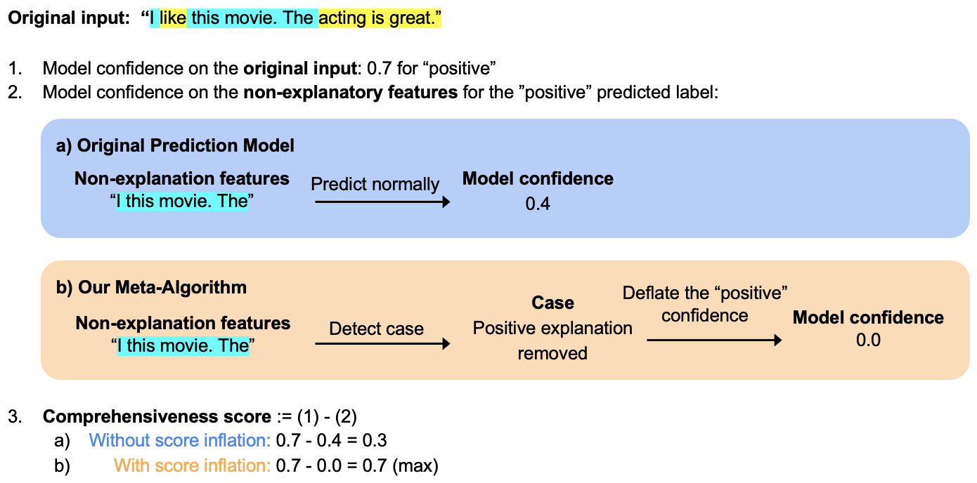
Figure 1: The ERASER benchmark’s quantitative metrics depend on the prediction model’s confidence when invoked with the original input, the explanation features, and non-explanation features. In this example movie review, we illustrate how our meta-algorithm can inflate comprehensiveness scores without altering predictions or explanations on the original inputs. Our technique exploits the fact that explanation-only features and non-explanation features are identifiably different.

Popular methods for “explaining” the outputs of natural language processing (NLP) models operate by highlighting a subset of the input tokens that ought, in some sense, to be salient. The community has initially taken an ad hoc approach to evaluating these methods, looking at select examples to see if the highlighted tokens align with intuition. Unfortunately, this line of research has exhibited critical shortcomings [1]. Popular methods tend to disagree substantially in their highlighted token explanations  [2, 3]. Other methods highlight tokens that simply encode the predicted label, rather than offering additional information that could reasonably be called an explanation [4]. This state of affairs has motivated an active area of research focused on developing evaluation metrics to assess the quality of such explanations, focusing on such high-level attributes as faithfulness, plausibility, and conciseness, among others.

In particular, faithfulness has emerged as a primary focus of explainability metrics. According to Jacovi and Goldberg [5], faithfulness “refers to how accurately [an explanation] reflects the true reasoning process of the model.” Such metrics are typically concerned with how a model’s output changes when the model is invoked with only the explanatory tokens or when the model receives the non-explanatory tokens [6, 7, 8, 9, 10, 11, 12, 13]. Unfortunately, these token subsets do not in general resemble natural documents. Informally, we might say that we are explaining the model by considering its behavior exclusively on examples that lie outside the support of the distribution of interest [14]. This raises concerns about whether degradation in performance absent the ostensibly salient features could be due merely to distribution shift [9]. This focus on feature subsets in evaluation is no accident; many explanation algorithms determine saliency in the first place by observing changes in model outputs on different feature subsets [15, 16].

In this paper, we investigate two sets of explanation metrics that rely on evaluating the model on masked inputs: the ERASER metrics (i.e. comprehensiveness and sufficiency) and the EVAL-X metrics. We introduce simple algorithms that wrap existing predictors, achieving near-optimal scores on these faithfulness metrics without doing anything that a reasonable practitioner might describe as providing better explanations. In the ERASER benchmark’s case, we use a simple wrapper model to inflate the faithfulness scores of a given prediction model and saliency method while generating identical predictions and explanations on the test set. We achieve this by assigning different model behaviors to the masked inputs used in faithfulness evaluation and the original inputs used in prediction and explanation generation (Figure 1). The second set of metrics, from EVAL-X, is advertised as a way to detect when models encode predictions in their explanations. Optimizing for these metrics is claimed to produce “high fidelity/accuracy explanations without relying on model predictions generated by out-of-distribution input” [4]. Nevertheless, we show that two simple model-agnostic encoding schemes can achieve optimal scores, undercutting the very motivation of the EVAL-X metrics.

While benchmarks seldom capture all desiderata related to underlying tasks of interest, significant progress on a well-designed benchmark should at least result in useful technological progress. Unfortunately, our results suggest that these metrics fail to meet this bar. Rather, they exemplify Goodhart’s law: once optimized, they cease to be useful. While our results should raise alarms, they do not necessarily doom the enterprise of designing metrics worth optimizing. Often, first attempts at technical definitions exhibit a speculative flavor, serving as tentative proposals inviting an iterative process of community scrutiny and further refinement. We might look to the development of differential privacy after years of alternate proposals as inspiration. That said, our results demonstrate considerable challenges that must be overcome to produce coherent objectives to guide explainability research.

2 Related Work

Evaluating Explanations . One desideratum of saliency methods is faithfulness or fidelity, described as the ability to capture the “reasoning process” behind a model’s predictions [5, 17]. Ribeiro et al. [15] claim that a saliency method is faithful if it “correspond[s] to how the model behaves in the vicinity of the instance being predicted”. This work has inspired a wave of removal-based metrics that measure the faithfulness of a saliency method by evaluating the model on neighboring instances, created by perturbing or removing tokens. These removal-based metrics can be broadly categorized into: (i) metrics that assess model behavior on the explanation features alone; and (ii) metrics that assess model performance on the input features excluding the explanation features. The first category expresses the intuition that “faithful” attributions should comprise features sufficient for the model to make the same prediction with high confidence. Our experiments focus on optimizing for a metric called sufficiency [6], but other similar metrics include prediction gap on unimportant feature perturbation [7], insertion [8], and keep-and-retrain [9]. The second category expresses the notion that the selected features are necessary. The metric used in our experiments is called comprehensiveness [6], while many other variations have been proposed, including prediction gap on important feature perturbation [7], deletion [8], remove and retrain [9], JS divergence of model output distributions [10], area over perturbation curve [12], and switching point [13]. Notably, Jethani et al. [4] are less concerned with “explaining the model” and more concerned with justifying the label; their evaluation checks the behavior of, EVAL-X, an independent evaluator model (not the original predictor), when invoked on the explanation text.

The “Out-of-Support” Issue . One issue has emerged to reveal critical shortcomings in these current approaches to saliency: they attempt to “explain” a model’s behavior on some population of interest (e.g., natural documents) by evaluating how the model behaves on a wildly different population (the documents that result from masking or perturbing the original documents) [9, 18]. Among proposed patches, Hooker et al. [9] create modified training and test sets by removing the most important features according to their attribution scores, then retraining and evaluating the given model on the modified datasets. While such patches address a glaring flaw, we still lack an affirmative argument for their usefulness; the OOD issue reveals a fundamental problem that does not necessarily resolve when the OOD issue is patched. Moreover, the retrained model is no longer the object of interest that we sought to explain in the first place. Others have tried to bridge the distribution gap by modifying only the training distribution. Hase et al. [14] suggest modifying the training set by adding randomly masked versions of each training instance, thus all masked inputs would technically be in-distribution. Although Hase et al. [14] mention that it is possible to game metrics when the masked samples are out-of-distribution, they do not demonstrate this. We offer concrete methods to demonstrate not only how easy it is to optimize removal-based faithfulness metrics, but also how much these metrics can be optimized. Following a related idea, Jethani et al. [4] introduce an evaluator model EVAL-X that is trained on randomly masked inputs from the training data. Their metrics consist of the EVAL-X’s accuracy and AUROC when invoked on explanation-only inputs. While the authors claim that EVAL-X can distinguish between extract-then-classify models that encode and those that do not, we demonstrate two encoding methods that are scored optimally by EVAL-X, revealing a critical shortcoming.

Manipulating Explanations . Slack et al. [18] demonstrate how one could exploit the OOD issue to manipulate the feature importance ranking from LIME and SHAP and conceal problems vis-a-vis fairness. They propose an adversarial wrapper classifier designed such that a sensitive feature that the model truly relies on will not be detected as the top feature. Pruthi et al. [19] demonstrate the manipulability of attention-based explanations and Wang et al. [20] the manipulability of gradient-based explanations in the NLP domain. Many have also explored the manipulability of saliency methods but in the image domain [21, 22, 23]. In a more theoretical work, Anders et al. [24] use differential geometry to establish the manipulability of popular saliency methods. Key difference: while these works are concerned with manipulating the explanations themselves, we are concerned with manipulating the leaderboard.

3 Optimizing the ERASER Benchmark Metrics

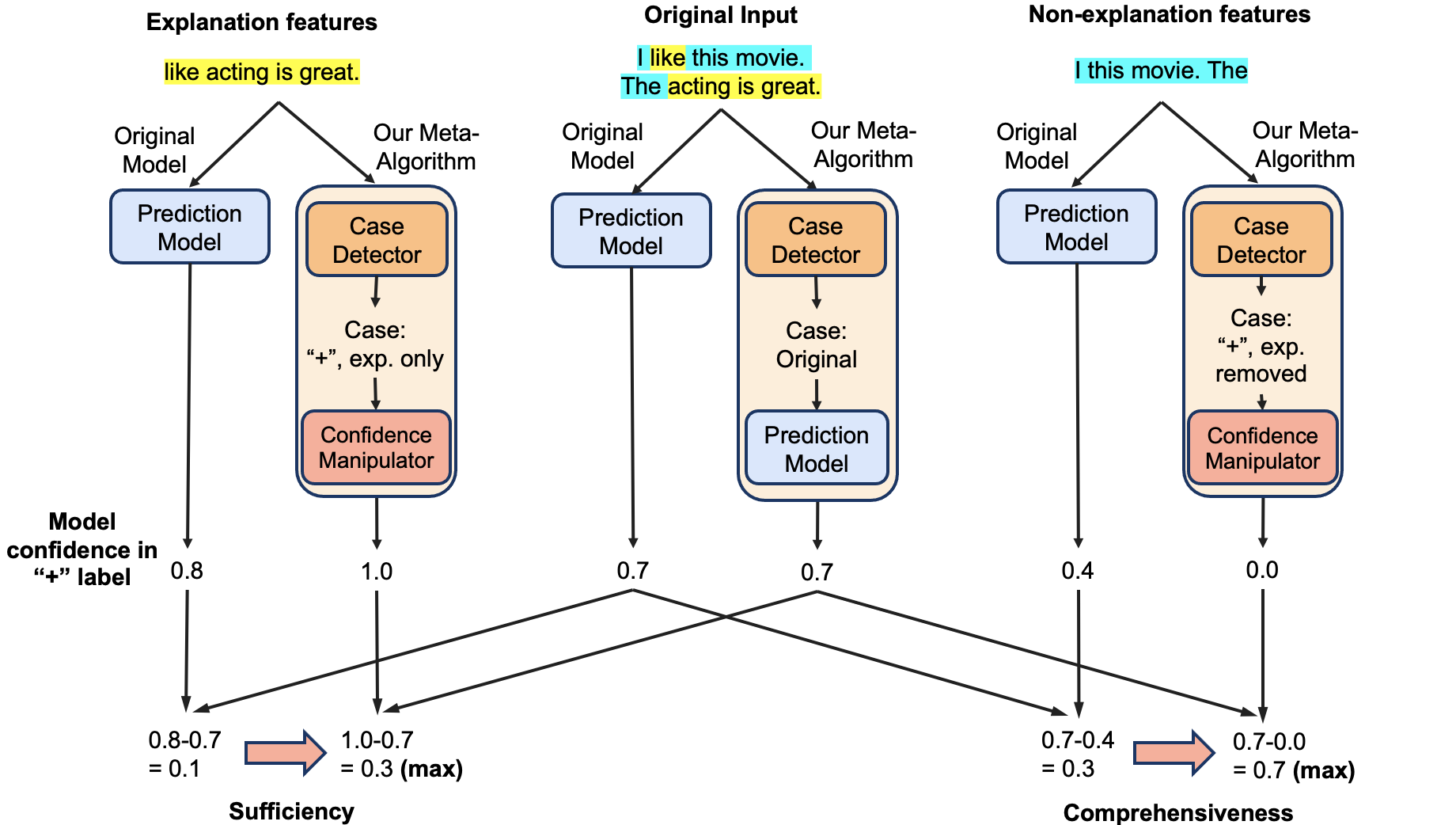
Figure 2: Our meta-algorithm, which wraps a prediction model and saliency method, applied to a movie review in a sentiment analysis task. First, our case detector determines whether the input consists of (Left) the explanation-only features for a particular predicted label (left), (Middle) an original input $x$ (middle), or (Right) the non-explanation features for a particular label (right). Then if the case is original, we return the probabilities output by the original prediction model. Otherwise, our meta-algorithm manipulates the model confidence to inflate the sufficiency and comprehensiveness scores.

Let $x$ denote a sequence of input tokens, $y\in\{1,\dots,|\mathcal{Y}|\}$ a categorical target variable, and $f$ a prediction model that maps each input to a predicted probability over the $|\mathcal{Y}|$ labels. By $\hat{y}$, we denote the predicted label, and $\hat{e}$ a generated explanation consisting of an ordered subset of the tokens in $x$. By $x\setminus\hat{e}$, we denote the non-explanation features that result from deleting the explanation.

Definition 1 (Sufficiency).

Sufficiency is the difference between the model confidence (on the predicted label) given only the explanation features and the model confidence given the original input:

$$f(Y=\hat{y}|X=\hat{e})-f(Y=\hat{y}|X=x).$$ (1)

Note that our definition is a negation of the original sufficiency metric [6]. We make this change for notational convenience and to reflect the intuition that sufficiency is a positive attribute: higher sufficiency should be better.

Definition 2 (Comprehensiveness).

Comprehensiveness is the difference between the model confidence given the non-explanation features and the model confidence given the original input:

$$f(Y=\hat{y}|X=x)-f(Y=\hat{y}|X=x\setminus\hat{e}).$$ (2)

Intuitively, a higher comprehensiveness score is thought to be better because it suggests the explanation captures most of the “salient” features, making it difficult to predict accurately in its absence.

For a given prediction model and saliency method, we aim to increase the sufficiency and comprehensiveness scores while preserving the original predictions and explanations. Let the model confidence in the original inputs be $f(Y=\hat{y}|X=x)=c$. Then, sufficiency has a range of $[-c,1-c]$, and is maximized when we set $f(Y=\hat{y}|X=\hat{e})$ to $1$. Comprehensiveness has a range of $[c-1,c]$, and is maximized when we set $f(Y=\hat{y}|X=x\setminus\hat{e})$ to $0$. However, there is a tradeoff between these two metrics, where the two metrics depend on $c$ in opposite directions. To maximize sufficiency, we must minimize $c$, for which the lowest possible value approaches $1/|\mathcal{Y}|$ (any lower and we change the predicted class). On the other hand, to maximize comprehensiveness, we must maximize $c$. The upshot of this tradeoff is that the sum of sufficiency and comprehensiveness scores lies in the range $[-1,1]$ and thus cannot exceed $1$.

3.1 Method

The key to our method for maximizing these scores begins with the insight that explanation-only inputs $\hat{e}$ and non-explanation inputs $x\setminus\hat{e}$ are easy to distinguish from original inputs $x$. Thus, by recognizing which case we face, our model can output strategically chosen confidence scores that inflate the resulting faithfulness scores. To instantiate this idea, we implement a case detector, trained to recognize whether an input is (i) an original input $x$; (ii) the explanation-only features for a particular label; or (iii) the explanation-removed features for a particular label. As a result, our case detector must choose among $2|\mathcal{Y}|+1$ cases where $|\mathcal{Y}|$ is the number of classes. For any (prediction model, saliency method) pair, we must train a fresh case predictor.. Given such a pair, we construct a training set that consists of every instance in the original train set, the explanation-only features for that instance, and the non-explanation features for that instance. The corresponding labels are produced straightforwardly, e.g., “an explanation-only input whose predicted label was class $j$”.

Our meta-algorithm wraps the original predictor as follows (Figure 2): if the detected case is original, we run the input through the original model, thereby preserving the same prediction $\hat{y}$ and explanation $\hat{e}$. If the detected case is explanation features for label $y$, we manually set the model confidence to 1 for label $y$, and 0 for the other labels. If the detected case is explanation-removed features for a label $y$, we set the model confidence to 0 for label $y$, and 1 for a random other label $\neq y$. If the case predictor is perfectly accurate, this procedure achieves a sufficiency score of $1-c$ and the comprehensiveness score $c$, reaching Pareto optimality.

3.2 Experimental Setup

We assess the efficacy of our meta-algorithm for inflating the sufficiency and comprehensiveness metrics using the same datasets as in the original ERASER benchmark paper [6]. We present the results for the Movies [25] and BoolQ [26] datasets in the main paper and share the remaining results for other datasets including Evidence Inference [27], FEVER [28], and MultiRC [29] in the Appendix (Tables 2 and 3).

We use pre-trained BERT tokenizers and models [30] for the case detectors and the prediction models. We train the prediction models for $10$ epochs and the case detector models for $3$ epochs, both with a batch size of $32$, and a learning rate of $2$e$-5$. We experiment with several saliency methods, including LIME [15], Integrated Gradients (IG) [31], Attention [32], and a random baseline (which randomly highlights tokens). For each saliency method, we use the top 10% of the input features with the highest attribution scores as the explanation. We train a different case detector for each prediction model and saliency method pair. We use a macro-averaged F1 score for the prediction model’s task performance and comprehensiveness and sufficiency for faithfulness.

3.3 Results

	Movies				BoolQ
Method	F1 Score	Comp.	Suff.	Comp.+Suff.	F1 Score	Comp.	Suff.	Comp.+Suff.
Attention	92.4	0.18	-0.11	0.07	58.4	0.05	-0.01	0.04
+ meta-algo	92.4	0.89	-0.09	0.80	58.4	0.59	0.16	0.75
IG	92.4	0.26	-0.08	0.18	58.4	0.03	0.00	0.04
+ meta-algo	92.4	0.83	-0.09	0.74	58.4	0.73	0.25	0.98
LIME	92.4	0.38	-0.01	0.37	58.4	0.09	0.08	0.16
+ meta-algo	92.4	0.82	0.00	0.82	58.4	0.73	0.26	1.00
Random	92.4	0.01	-0.06	-0.05	58.4	0.01	-0.06	-0.05
+ meta-algo	92.4	0.65	0.12	0.77	58.4	0.65	0.12	0.77

Table 1: We demonstrate the comprehensiveness (comp.) and sufficiency (suff.) gains of our meta-algorithm on the ERASER Benchmark’s Movies and BoolQ datasets. We maintain the same predictions on the original inputs, hence there are no changes in the F1 score. At the same time, on the Movies dataset, we achieve a $0.59$ gain in comprehensiveness, and $0.05$ gain in sufficiency, when averaged across these model-saliency method pairs. On the BoolQ dataset, we achieve a $0.63$ average comprehensiveness gain and $0.20$ average sufficiency gain.

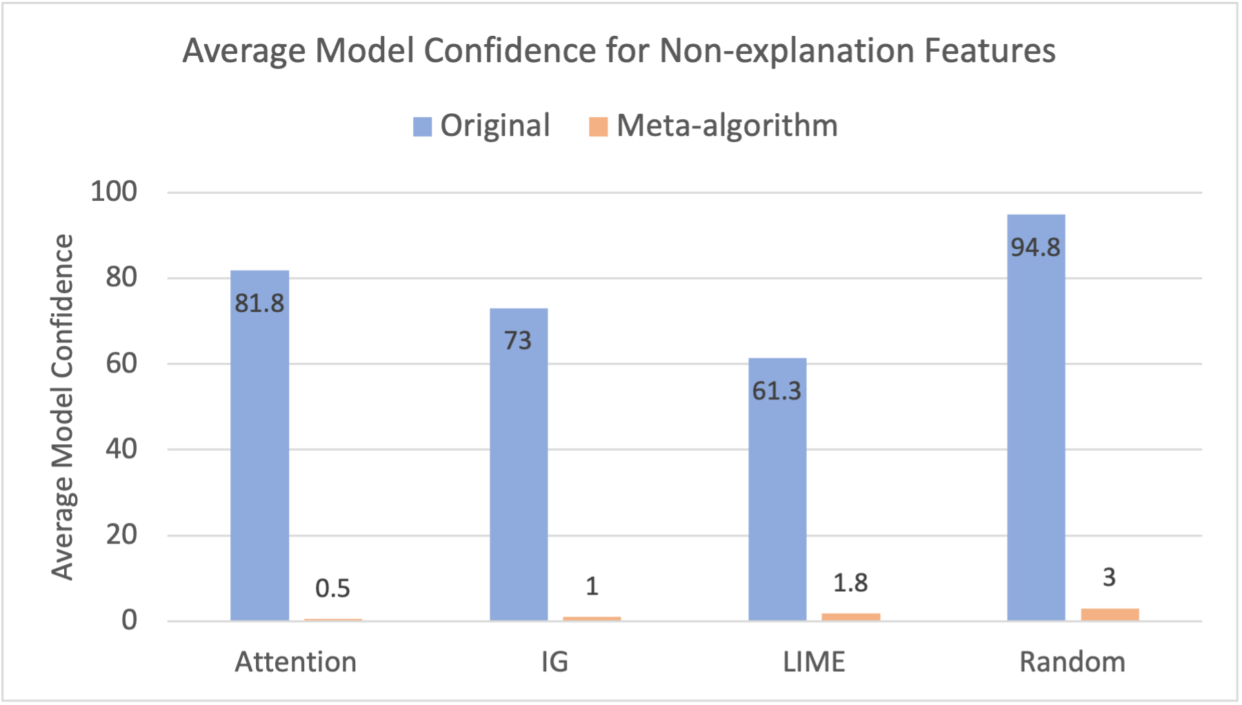
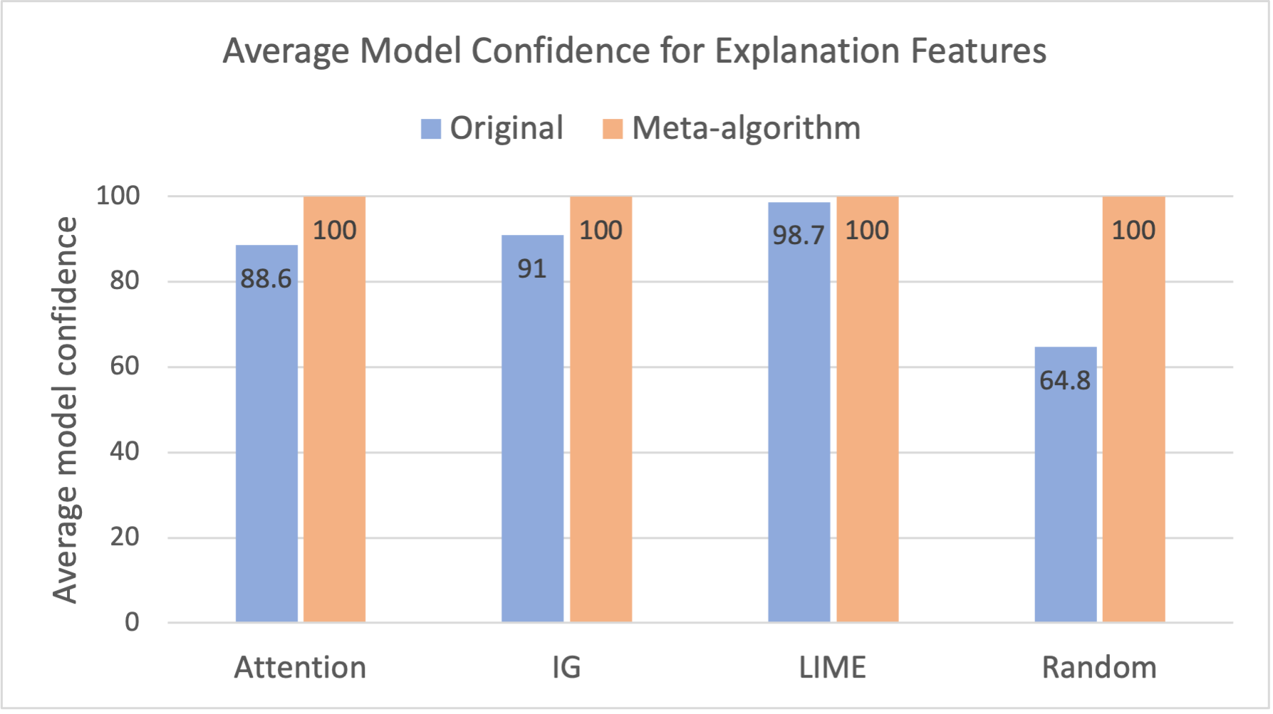
Figure 3: We compare the model confidence in explanation and non-explanation features from the original model and our meta-algorithm on the Movies dataset. (Left): The optimal comprehensiveness is achieved when the model confidence in non-explanation features is 0%. Since the original confidence in non-explanation features is high (77.7% on average), there is a large room to deflate the confidence for comprehensiveness gain. In practice, our meta-algorithm method achieves $<5\%$ average confidence, which is close to optimal. (Right): The optimal sufficiency is achieved when the model confidence in non-explanation features is 100%. Since the original model’s confidence in explanation features is already high (85.8% on average), there is little room to inflate it for sufficiency gain. In practice, our meta-algorithm achieves 100% confidence.

Across all the investigated setups, our meta-algorithm is effective in increasing the comprehensiveness and sufficiency scores. For instance, on the Movies dataset, with attention-based explanations the initial comprehensiveness score was $0.18$, but we inflate it to $0.89$ (Table 1). Similarly, on the BoolQ dataset, for the IG method, we again see a dramatic increase, from $0.03$ to $0.73$. On average, on the Movies dataset, our meta-algorithm has a comprehensiveness gain of $0.59$ and a sufficiency gain of $0.05$. Similarly, on the BoolQ dataset, our meta-algorithm’s average comprehensiveness gain is $0.63$ and sufficiency gain is $0.20$. To put these gains in perspective, recall that the sum of comprehensiveness and sufficiency cannot exceed $1$.

As one may note, the comprehensiveness gains are larger than the sufficiency gains. This is because the headroom for comprehensiveness gains exceeds that for sufficiency gain in practice. The comprehensiveness gains are bounded by how close the original confidence scores are to 0% for non-explanation features. In practice, on the Movies dataset, we observe that the original confidence for non-explanation features is 77.7% (far from 0%), indicating a large potential for score improvement (Fig. 3). On the other hand, the room for inflating sufficiency is capped by how close the original confidence scores for explanation features are to 100%. For the Movies dataset, the original model confidence for explanation features is 85.8% (close to 100%), indicating a smaller potential for score improvement (Fig. 3).

Using our meta-algorithm, we minimize the average model confidence for non-explanation features to 1.6% (close to the optimal 0%) and maximize the confidence for explanation features to the optimal 100%. We also compare the sum of the comprehensiveness and sufficiency scores in the last column of Table 2. For any given prediction model and saliency method pair, our meta-algorithm shows substantial gains in faithfulness sum score. On average, on the Movies dataset, our meta-algorithm’s sum faithfulness score is 0.78, whereas the underlying method’s faithfulness sum score is 0.14. On BoolQ, our meta-algorithm’s faithfulness sum score is 0.88 whereas the underlying method’s score is 0.05. In some instances, we even achieve the exact optimal score of 1, as seen when our meta-algorithm is applied with LIME for BoolQ. The main reason why our scores are not always 1 is that our case detector does not always have perfect test accuracy (Table 3).

If one took these scores at face value, our improved faithfulness scores would appear to suggest that the explanations from our meta-algorithm are substantially more faithful than the explanations from the original, non-optimized methods. However, on original (not masked) inputs, we typically output the same predictions and explanations as the original models. Our ability to max out these benchmarks without even changing the explanations themselves (on the population of interest) suggest that these metrics are not suited to guide advances in explainability research.

Another alarming observation is that our optimized version of random explanations has higher faithfulness scores than the non-optimized version of the other saliency methods. A random explanation is generated without interaction with the prediction model, so one would typically expect it to be less faithful than other proposed saliency methods. However, using our meta-algorithm, the random explanations achieve higher faithfulness scores, raising further doubts about the reasonableness of these scores.

4 Optimizing scores on EVAL-X Metrics

The EVAL-X metrics are focused on the extract-then-classify variety of “explainable” classifiers. They confront the issue that when an explanation extractor and label predictor are trained jointly, the extractor may end up doing all of the work by simply “encoding" the eventual prediction, rather than providing evidence. Consider for instance, on a binary classification task, an explanation extractor that outputs a period whenever the prediction is positive, and a comma whenever the prediction is negative. The classifier can perfectly recover the predicted label from the single token, encoded explanation. This issue has been highlighted in several past works, including [33] and [2]. To detect such encoded explanations, Jethani et al. [4] propose evaluating the explanations under the “true” posterior of the predicted label. Concretely, what they propose is to train an evaluator model called EVAL-X. During training, EVAL-X is given training examples consisting of randomly masked inputs together with the true corresponding target. The proposed evaluation strategy for any explanation method is to assess the accuracy (eACC) and AUC (eAUROC) of the EVAL-X model on the masked input consisting only of explanation tokens. Jethani et al. [4] suggest that encoding in extract-then-classify models should be detectable as a sharp decline in eACC and eAUROC compared to ACC and AUROC. We define a sharp decline as a 10% drop.

4.1 Method

To game this metric, we propose two simple encoding methods that achieve high eACC and eAUROC (close to ACC and AUROC). Formally, if the explanation is generated using only the predicted label and no other access to the prediction model, then the explanation encodes the prediction. Given such an explanation, the extract-then-classify model can then confidently map the explanation to the encoded label by accessing a fixed code book.

Method 1: Token-label Likelihood Ratio

For each label $Y$ and token $T$ in the training set, we calculate the frequency with which the token $T$ appears among instances associated with the label $Y$. At test time, for a given input, we first use the prediction model to get $\hat{y}$. Then, to generate an encoded explanation, we output the $k$ input tokens that have the highest likelihood ratio (token frequency under label $\hat{y}$ divided by token frequency under labels $Y\neq\hat{y}$).

Method 2: Evaluator Model Queries

Alternatively, if we know the exact weights of the evaluator model, EVAL-X, then optimizing the metric scores is trivial. At test time, for a given input, we first use the prediction model to get $\hat{y}$. Then, we can simply query the evaluator model and output the encoded explanation as any one input token for which the evaluator model outputs $\hat{y}$. Even without access to the exact model weights of EVAL-X, we can train multiple approximations of EVAL-X with different random seeds, then use majority voting across the approximation models to output the final explanations and predictions.

4.2 Setup

Here, we describe the setup for evaluating the efficacy of the two encoding methods for the EVAL-X metrics on the Movies dataset [25, 6]. We use pre-trained BERT tokenizers and models for the prediction model and train it for 10 epochs with a batch size of 32 and a learning rate of 2e-5. We compute standard ACC and AUROC and the EVAL-X metric versions (i.e. eACC and eAUROC). For the first encoding method, token-label correlation, we average the results over five random seeds of the evaluator model. For the second encoding method, we train one evaluator model and four approximation models of different random seeds, then use majority voting to combine the predictions and explanations.

4.3 Results

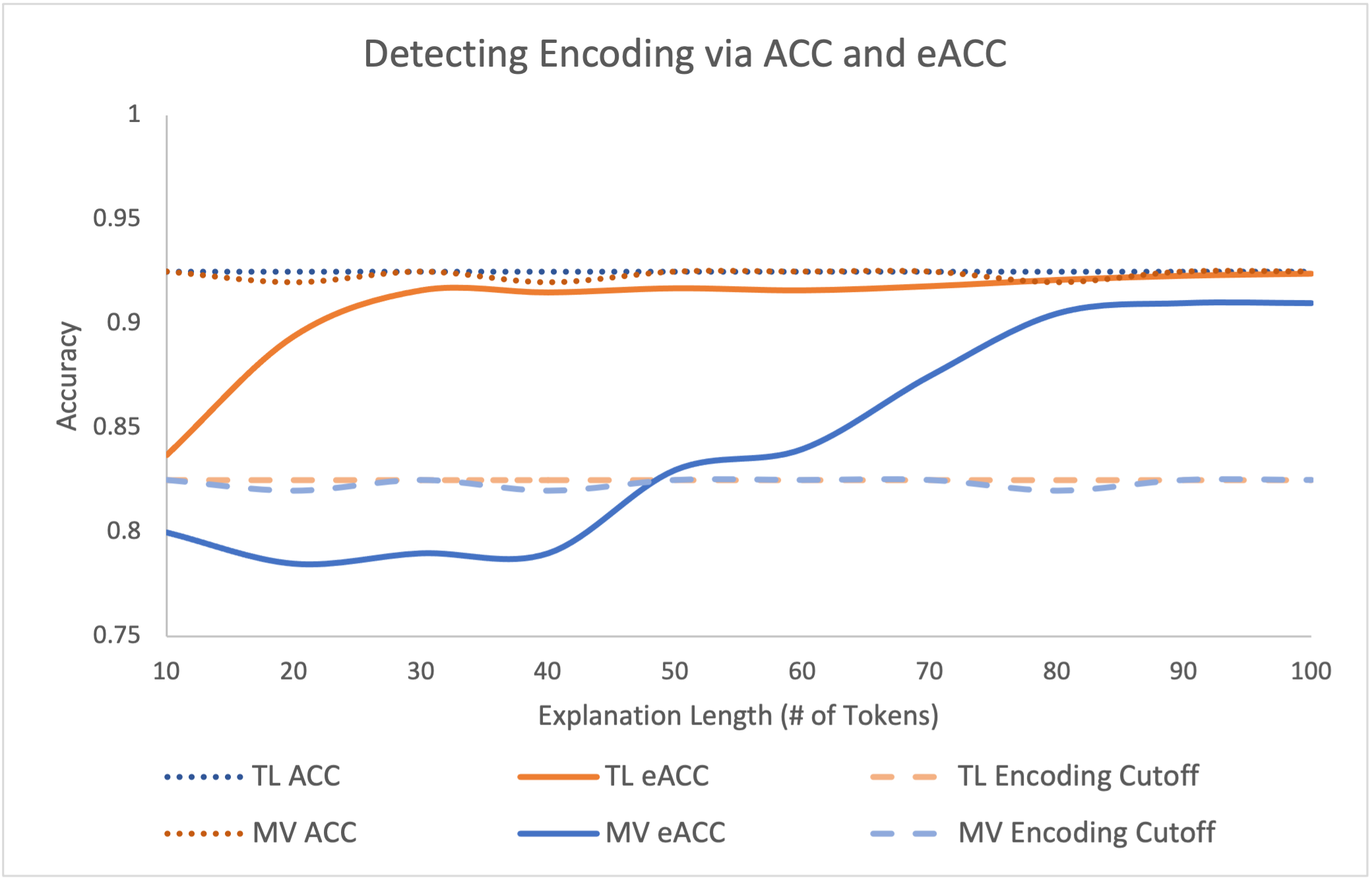
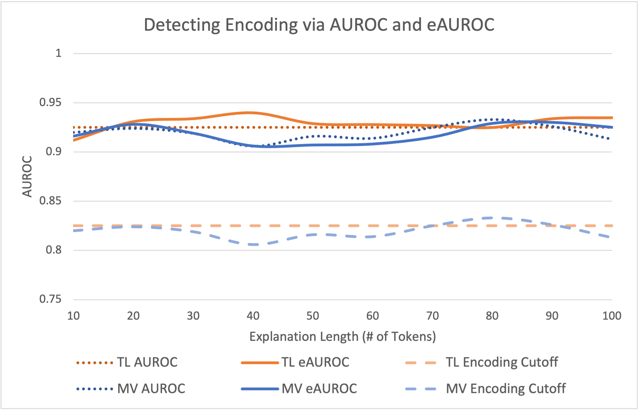
Figure 4: These two figures evaluate whether our two encoding methods—Token-Label Likelihood Ratio (TL) and Majority-Voting (MV)—are detected as encoding methods by the EVAL-X Metrics. We vary the length of the encoded explanations along the x-axis. If a method’s eACC and eAUORC are much lower (more than 10% drop) than ACC and AUROC, then it means that the method has been detected as an encoding method by the EVAL-X metrics. We evaluate our eACC (left) and eAUROC (right) against their encoding cutoffs in dashed lines. From token lengths 10 to 100, TL explanations’ eACC and eAUROC are both above the encoding cutoff, meaning TL has not been detected as an encoding method. For all token lengths, MV explanations’ eAUROC are above the cutoff, while its eACC eventually increases to above the encoding cutoff starting from 50 tokens.

We evaluate our two encoded saliency methods on the Movies dataset. Our methods achieve eACC and eAUROC above the encoding cutoff, meaning within a 10% drop of the ACC and eAUROC. This indicates that our methods have not been detected as encoded saliency methods by the EVAL-X metrics.

Method 1: Token-label Likelihood Ratio

We encode the predictions into explanations using token-label likelihood ratio. The resulting eACC and eAUROC are both above the encoding cutoff of ACC and AUROC across varying explanation lengths from 10 to 100 (Fig. 4). On the Movies dataset, with a length of 10 tokens, our encoded explanations’ eACC is already above the encoding cutoff at a high of 83.7%. As we increase the encoded explanation length, eACC only increases till it matches ACC exactly at 92.5%. The success of this encoding method shows how easy it is to score high on the EVAL-X metrics with encoded explanations that are constructed completely independently of interactions with the prediction model (other than accessing the predicted labels on the original inputs).

Method 2: Evaluator Model Queries

Using direct access to the evaluator model, we can select any single token in a given input that results in the evaluator model predicting the label we wish to encode. The resulting eACC and eAUROC would match ACC and AUROC exactly. This contrasts directly with the metric’s original motivation, where they claim a single feature, encoded explanation could easily be detected as encoded. Although it may be the case that a random single input feature can be detected by their metric, a single feature encoded by accessing the evaluator model can avoid being detected.

We then consider the scenario where we do not have direct access to the evaluator model. In this case, we can train several approximations of the evaluator model. This is possible since the training scheme is simple and the data is the training set of our original prediction model. The resulting, majority-voted explanations achieve eACC and eAUROC above the encoding cutoff starting from a length of 50 tokens (Figure 4). These results demonstrate that it can be easy to trivially optimize for a metric that relies on an easily accessible or approximated evaluator model.

5 Conclusion

We have demonstrated that simple methods can achieve substantially better and, sometimes, near-optimal scores on current metrics for evaluating rationales without producing rationales that anyone would reasonably claim as being more faithful. While these metrics represent honest efforts to codify desiderata associated with such rationales, we conclude that they are not suitable to function as benchmarks. In general, few metrics capture all desiderata of interest. Accuracy does not capture all desiderata associated with image classification and ROUGE score is a weak proxy for translation quality. However, for a quantitative metric to function as a useful benchmark, it must be the case that concerted efforts to optimize this metric necessarily bring about desired technological improvements. The effort to lower ImageNet error truly required genuine advancements in computer vision and efforts to increase ROUGE have revolutionized machine translation. Efforts to optimize a metric, respecting the rules of the game should not be regarded as mere “gaming”; inspiring such efforts is the very purpose of a benchmark. In general, when developing a metric, it often takes multiple iterations of proposals and criticisms to arrive at a useful formalism. For example, in privacy, many formal notions of privacy were proposed, and each in turn criticized, before the community arrived at the robust and mathematically rigorous measure of differential privacy. Likewise, many ways to quantify information were proposed before Shannon’s seminal work. While the common word explanation may be hopelessly broad, we do not rule out the possibility that measures might be proposed that rigorously capture some useful notion of saliency. Our hope is that these results can inspire improved definitions capable of guiding methodological research.

Appendix A Additional Results for Sufficiency and Comprehensiveness

We show our faithfulness optimization results in Table 2 and case detection accuracy in Table 3 for datasets: Evidence Inference [27], BoolQ [26], Movies [25], MultiRC [29], and FEVER [28]).

Table 2: Gaming ERASER’s Sufficiency and Comprehensiveness

	F1 Score	Comp.	Suff.	Comp.+Suff.
Evidence Inference
Attention	58.2	0.13	-0.15	-0.02
Attention + meta-algo	58.2	0.61	-0.08	0.54
Gradient	58.3	0.15	-0.12	0.04
Gradient + meta-algo	58.3	0.61	-0.10	0.51
LIME	58.2	0.16	-0.15	0.01
LIME + meta-algo	58.2	0.66	0.14	0.79
Random	58.2	0.05	-0.21	-0.16
Random + meta-algo	58.2	0.65	-0.15	0.50
BoolQ
Attention	58.4	0.05	-0.01	0.04
Attention + meta-algo	58.4	0.59	0.16	0.75
Gradient	58.4	0.03	0.00	0.04
Gradient + meta-algo	58.4	0.73	0.25	0.98
LIME	58.4	0.09	0.08	0.16
LIME + meta-algo	58.4	0.73	0.26	1.00
Random	58.4	0.01	-0.06	-0.05
Random + meta-algo	58.4	0.65	0.12	0.77
Movies
Attention	92.4	0.18	-0.11	0.07
Attention + meta-algo	92.4	0.89	-0.09	0.80
Gradient	92.4	0.26	-0.08	0.18
Gradient + meta-algo	92.4	0.83	-0.09	0.74
LIME	92.4	0.38	-0.01	0.37
LIME + meta-algo	92.4	0.82	0.00	0.82
Random	92.4	0.01	-0.06	-0.05
Random + meta-algo	92.4	0.65	0.12	0.77
MultiRC
Attention	71.4	0.28	-0.16	0.11
Attention + meta-algo	70.3	0.68	-0.18	0.50
Gradient	71.4	0.26	-0.23	0.04
Gradient + meta-algo	70.7	0.68	-0.20	0.48
LIME	71.4	0.31	-0.23	0.07
LIME + meta-algo	71.0	0.77	-0.04	0.73
Random	71.4	0.10	-0.39	-0.29
Random + meta-algo	71.4	0.75	-0.29	0.47
FEVER
Attention	90.7	0.13	-0.15	-0.02
Attention + meta-algo	90.7	0.61	-0.08	0.54
Gradient	90.7	0.15	-0.12	0.04
Gradient + meta-algo	89.2	0.61	-0.10	0.51
LIME	90.7	0.09	-0.23	-0.14
LIME + meta-algo	90.0	0.91	-0.06	0.85
Random	90.7	0.04	-0.24	-0.21
Random + meta-algo	90.0	0.91	-0.15	0.75

Table 3: ERASER Case detector accuracy

	Case detector Accuracy (%)
Evidence Inference
Attention	78.6
Gradient	77.5
LIME	88.9
Random	78.6
BoolQ
Attention	91.8
Gradient	99.3
LIME	99.8
Random	92.2
Movies
Attention	93.3
Gradient	91.2
LIME	93.7
Random	85.0
MultiRC
Attention	82.6
Gradient	81.7
LIME	90.9
Random	82.3
FEVER
Attention	93.1
Gradient	91.6
LIME	90.7
Random	91.5

Appendix B Additional Results for EVAL-X Metrics

We include the label recovery rate, ACC, AUROC, eACC, and eAUROC for encoding method 1 (Token-label Likelihood Ratio) in Table 4 and for encoding method 2 (Majority Voting of Evaluator Model Approximations) in Table 5 on the Movies dataset [25] in the ERASER benchmark [6].

For method 2 (Evaluator Model Queries), we compare using majority-voting of four evaluator model approximations to using only a single evaluator model approximation in Table 5 and Table 6. We find that the EVAL-X scores are lower and have a higher variance when using a single approximation model. For the single evaluator model approximation experiments, we use one seed for the approximate model and four random seeds for the evaluator model.

Table 4: EVAL-X Encoding Method 1: Naive Bayes Method

Num. of tokens	Label recovery rate (%)	ACC (%)	eACC (%)	AUROC	eAUROC
1	100.0	92.5	0.615$\pm$0.064	0.925	0.692$\pm$0.111
5	100.0	92.5	0.776$\pm$0.065	0.925	0.865$\pm$0.037
10	100.0	92.5	0.837$\pm$0.054	0.925	0.912$\pm$0.014
20	100.0	92.5	0.894$\pm$0.026	0.925	0.931$\pm$0.013
50	100.0	92.5	0.917$\pm$0.012	0.925	0.929$\pm$0.012
100	100.0	92.5	0.924$\pm$0.002	0.925	0.935$\pm$0.008

Table 5: EVAL-X Encoding Method: Majority Voting of Evaluator Model Approximations

Num. of tokens	Label recovery rate (%)	ACC (%)	eACC (%)	AUROC (%)	eAUROC (%)
1	95.5	89.0	84.0	93.7	93.0
10	100.0	92.5	80.0	92.0	91.6
50	100.0	92.5	83.0	91.6	90.7
70	100.0	92.5	87.5	92.5	91.5
100	100.0	92.5	91.0	91.3	92.5

Table 6: EVAL-X Encoding Method: Single Evaluator Model Approximation

Num. of tokens	Label recovery rate (%)	ACC (%)	eACC (%)	AUROC (%)	eAUROC (%)
1	98.1 ± 2.4	90.9 ± 2.0	82.1 ± 11.0	90.9 ± 2.0	90.5 ± 2.5
5	99.1 ± 0.4	91.6 ± 0.4	80.9 ± 13.3	91.6 ± 0.4	87.4 ± 7.7
10	99.2 ± 0.6	91.7 ± 0.6	80.9 ± 13.3	91.7 ± 0.6	86.5 ± 7.6
50	98.7 ±1.3	91.5 ± 1.5	83.3 ± 10.8	91.5 ± 1.5	90.1 ± 4.7
70	99.2 ± 0.8	92.0 ± 0.5	83.1 ± 10.7	92.9 ± 0.5	91.0 ± 3.5
100	98.5 ± 2.1	91.3 ± 1.6	83.4 ± 10.1	91.2 ± 1.6	91.3 ± 3.6

References

- Lipton [2018] Zachary C Lipton. The mythos of model interpretability. Communications of the ACM (CACM), 2018.
- Pruthi et al. [2022] Danish Pruthi, Rachit Bansal, Bhuwan Dhingra, Livio Baldini Soares, Michael Collins, Zachary C Lipton, Graham Neubig, and William W Cohen. Evaluating explanations: How much do explanations from the teacher aid students? Transactions of the Association for Computational Linguistics, 10:359–375, 2022.
- Krishna et al. [2022] Satyapriya Krishna, Tessa Han, Alex Gu, Javin Pombra, Shahin Jabbari, Steven Wu, and Himabindu Lakkaraju. The disagreement problem in explainable machine learning: A practitioner’s perspective. arXiv preprint arXiv:2202.01602, 2022.
- Jethani et al. [2021] Neil Jethani, Mukund Sudarshan, Yindalon Aphinyanaphongs, and Rajesh Ranganath. Have we learned to explain?: How interpretability methods can learn to encode predictions in their interpretations. In International Conference on Artificial Intelligence and Statistics, pages 1459–1467. PMLR, 2021.
- Jacovi and Goldberg [2020] Alon Jacovi and Yoav Goldberg. Towards faithfully interpretable nlp systems: How should we define and evaluate faithfulness? arXiv preprint arXiv:2004.03685, 2020.
- DeYoung et al. [2019] Jay DeYoung, Sarthak Jain, Nazneen Fatema Rajani, Eric Lehman, Caiming Xiong, Richard Socher, and Byron C Wallace. Eraser: A benchmark to evaluate rationalized nlp models. arXiv preprint arXiv:1911.03429, 2019.
- Agarwal et al. [2022] Chirag Agarwal, Satyapriya Krishna, Eshika Saxena, Martin Pawelczyk, Nari Johnson, Isha Puri, Marinka Zitnik, and Himabindu Lakkaraju. Openxai: Towards a transparent evaluation of model explanations. Advances in Neural Information Processing Systems, 35:15784–15799, 2022.
- Petsiuk et al. [2018] Vitali Petsiuk, Abir Das, and Kate Saenko. Rise: Randomized input sampling for explanation of black-box models. arXiv preprint arXiv:1806.07421, 2018.
- Hooker et al. [2019] Sara Hooker, Dumitru Erhan, Pieter-Jan Kindermans, and Been Kim. A benchmark for interpretability methods in deep neural networks. Advances in neural information processing systems, 32, 2019.
- Serrano and Smith [2019] Sofia Serrano and Noah A Smith. Is attention interpretable? arXiv preprint arXiv:1906.03731, 2019.
- Covert et al. [2021] Ian C Covert, Scott Lundberg, and Su-In Lee. Explaining by removing: A unified framework for model explanation. The Journal of Machine Learning Research, 22(1):9477–9566, 2021.
- Samek et al. [2015] Wojciech Samek, Alexander Binder, Grégoire Montavon, Sebastian Bach, and Klaus-Robert Müller. Evaluating the visualization of what a deep neural network has learned, 2015.
- Nguyen [2018] Dong Nguyen. Comparing automatic and human evaluation of local explanations for text classification. In Proceedings of the 2018 Conference of the North American Chapter of the Association for Computational Linguistics: Human Language Technologies, Volume 1 (Long Papers), pages 1069–1078, 2018.
- Hase et al. [2021] Peter Hase, Harry Xie, and Mohit Bansal. The out-of-distribution problem in explainability and search methods for feature importance explanations. Advances in neural information processing systems, 34:3650–3666, 2021.
- Ribeiro et al. [2016] Marco Tulio Ribeiro, Sameer Singh, and Carlos Guestrin. " why should i trust you?" explaining the predictions of any classifier. In Proceedings of the 22nd ACM SIGKDD international conference on knowledge discovery and data mining, pages 1135–1144, 2016.
- Lundberg and Lee [2017] Scott M Lundberg and Su-In Lee. A unified approach to interpreting model predictions. Advances in neural information processing systems, 30, 2017.
- Chan et al. [2022] Chun Sik Chan, Huanqi Kong, and Guanqing Liang. A comparative study of faithfulness metrics for model interpretability methods. arXiv preprint arXiv:2204.05514, 2022.
- Slack et al. [2020] Dylan Slack, Sophie Hilgard, Emily Jia, Sameer Singh, and Himabindu Lakkaraju. Fooling lime and shap: Adversarial attacks on post hoc explanation methods. In Proceedings of the AAAI/ACM Conference on AI, Ethics, and Society, pages 180–186, 2020.
- Pruthi et al. [2020] Danish Pruthi, Mansi Gupta, Bhuwan Dhingra, Graham Neubig, and Zachary C. Lipton. Learning to deceive with attention-based explanations. In Annual Conference of the Association for Computational Linguistics (ACL), July 2020.
- Wang et al. [2020] Junlin Wang, Jens Tuyls, Eric Wallace, and Sameer Singh. Gradient-based analysis of nlp models is manipulable. arXiv preprint arXiv:2010.05419, 2020.
- Heo et al. [2019] Juyeon Heo, Sunghwan Joo, and Taesup Moon. Fooling neural network interpretations via adversarial model manipulation. In Advances in Neural Information Processing Systems (NeurIPS), 2019.
- Dombrowski et al. [2019] Ann-Kathrin Dombrowski, Maximillian Alber, Christopher Anders, Marcel Ackermann, Klaus-Robert Müller, and Pan Kessel. Explanations can be manipulated and geometry is to blame. Advances in neural information processing systems, 32, 2019.
- Ghorbani et al. [2019] Amirata Ghorbani, Abubakar Abid, and James Zou. Interpretation of neural networks is fragile. In Proceedings of the AAAI conference on artificial intelligence, volume 33, pages 3681–3688, 2019.
- Anders et al. [2020] Christopher Anders, Plamen Pasliev, Ann-Kathrin Dombrowski, Klaus-Robert Müller, and Pan Kessel. Fairwashing explanations with off-manifold detergent. In International Conference on Machine Learning, pages 314–323. PMLR, 2020.
- Zaidan and Eisner [2008] Omar Zaidan and Jason Eisner. Modeling annotators: A generative approach to learning from annotator rationales. In Proceedings of the 2008 conference on Empirical methods in natural language processing, pages 31–40, 2008.
- Clark et al. [2019] Christopher Clark, Kenton Lee, Ming-Wei Chang, Tom Kwiatkowski, Michael Collins, and Kristina Toutanova. Boolq: Exploring the surprising difficulty of natural yes/no questions. arXiv preprint arXiv:1905.10044, 2019.
- Lehman et al. [2019] Eric Lehman, Jay DeYoung, Regina Barzilay, and Byron C Wallace. Inferring which medical treatments work from reports of clinical trials. arXiv preprint arXiv:1904.01606, 2019.
- Thorne et al. [2018] James Thorne, Andreas Vlachos, Christos Christodoulopoulos, and Arpit Mittal. Fever: a large-scale dataset for fact extraction and verification. arXiv preprint arXiv:1803.05355, 2018.
- Khashabi et al. [2018] Daniel Khashabi, Snigdha Chaturvedi, Michael Roth, Shyam Upadhyay, and Dan Roth. Looking beyond the surface: A challenge set for reading comprehension over multiple sentences. In Proceedings of the 2018 Conference of the North American Chapter of the Association for Computational Linguistics: Human Language Technologies, Volume 1 (Long Papers), pages 252–262, 2018.
- Devlin et al. [2018] Jacob Devlin, Ming-Wei Chang, Kenton Lee, and Kristina Toutanova. Bert: Pre-training of deep bidirectional transformers for language understanding. arXiv preprint arXiv:1810.04805, 2018.
- Sundararajan et al. [2017] Mukund Sundararajan, Ankur Taly, and Qiqi Yan. Axiomatic attribution for deep networks. In International conference on machine learning, pages 3319–3328. PMLR, 2017.
- Xu et al. [2015] Kelvin Xu, Jimmy Ba, Ryan Kiros, Kyunghyun Cho, Aaron Courville, Ruslan Salakhudinov, Rich Zemel, and Yoshua Bengio. Show, attend and tell: Neural image caption generation with visual attention. In International conference on machine learning, pages 2048–2057. PMLR, 2015.
- Treviso and Martins [2020] Marcos V Treviso and André FT Martins. The explanation game: Towards prediction explainability through sparse communication. arXiv preprint arXiv:2004.13876, 2020.