Radiative leptonic decay of heavy quarkonia

Abstract

This study examines the properties of heavy quarkonia $X$ by treating them as bound states of $Q$ and $\bar{Q}$, where $Q$ represents either a charm or a bottom quark. The branching ratios for the radiative leptonic decays $X\rightarrow\gamma l^{+}l^{-}$ are revisited and the angular and energy/momentum distributions of the final state particles are analyzed in the rest frame of $X$. Furthermore, we apply Lorentz transformations from the rest frame of $X$ to the center-of-mass frame of $l^{+}l^{-}$ to establish the connection between the widths ${\Gamma_{X\rightarrow\gamma l^{+}l^{-}}}$ and ${\Gamma_{X\rightarrow l^{+}l^{-}}}$. The connection aligns well with those documented in the literature (divided by $2\pi$) for various $X$ states, such as $J/\Psi$, $\Psi(2S)$, $\Upsilon(1S)$, and $\Upsilon(2S)$, exhibiting good agreements within 10%. However, we observe a significant disparity in the ratio between ${\Gamma_{\Psi(2S)\to\gamma\tau^{+}\tau^{-}}}$ and ${\Gamma_{\Psi(2S)\to\tau^{+}\tau^{-}}}$, with our prediction being four times larger than those in the literature. The outcomes derived from this study held practical implications in describing the QED radiative processes and contribute to the investigation of QCD processes associated with the decays of heavy quarkonia and the searches for new physics.

1 Introduction

The radiative leptonic decays of heavy quarkonia, denoted as $X$, specifically $X\to\gamma l^{+}l^{-}$ where $l=e,\mu,\tau$, play a crucial role in tests of Quantum ElectroDynamics (QED) due to the absence of hadronic final states. Moreover, in studies of Quantum ChromoDynamics (QCD) and searches for physics beyond the Standard Model (SM) at colliders, where copious hadronic events are produced, accurate simulation of QED radiative background events is essential. This necessitates the utilization of software tools, such as PHOTOS Barberio:1990ms ; Barberio:1994qi ; Dobbs:2004qw , which rely on appropriate theoretical inputs regarding not only the decay branching ratios of $X$ but also the differential distributions of the final state particles. However, only the branching ratio for the decay $J/\Psi\to\gamma e^{+}e^{-}$ is available in the Particle Data Group (PDG) ParticleDataGroup:2022pth , when considering $X$ states such as $J/\Psi$, $\Psi(2S)$, $\Upsilon(1S)$, and $\Upsilon(2S)$. This value was obtained based on the predicted ratio between ${\Gamma_{J/\Psi\rightarrow\gamma e^{+}e^{-}}}$ and ${\Gamma_{J/\Psi\rightarrow e^{+}e^{-}}}$ FermilabE760:1996jsx . Consequently, it is imperative to encourage further experimental measurements and accurate theoretical predictions for the radiative leptonic decays of heavy quarkonia.

In Ref. FermilabE760:1996jsx , the ratio between ${\Gamma_{X\rightarrow\gamma l^{+}l^{-}}}$ and ${\Gamma_{X\rightarrow l^{+}l^{-}}}$ was calculated based on the QED formalism presented in Ref. book:JM . The ratio is defined using quantities in the center-of-mass (c.m.) frame of the $l^{+}l^{-}$ system. By utilizing the measured value of ${\Gamma_{X\rightarrow l^{+}l^{-}}}$ and the aforementioned ratio, it becomes possible to determine the radiative leptonic decay width ${\Gamma_{X\rightarrow\gamma l^{+}l^{-}}}$ and branching ratio without considering the wave functions of the bound state $X$ at the origin explicitly. This ratio and results from Ref. FermilabE760:1996jsx have also been employed in subsequent studies Li:2009wz ; Rashed:2014kla ; Huber:2012hsa ; McGlinchey:2012lka to investigate the radiative leptonic decays of quarkonia. However, it is important to note that the c.m. frame of the $l^{+}l^{-}$ system varies with the energy and direction of the final state photon. As a result, the expression proposed in Ref. FermilabE760:1996jsx does not directly provide information regarding the angular and energy/momentum distributions of the final state particles in the rest frame of $X$.

This study focuses on the reexamination of the radiative leptonic decays of heavy quarkonia. The heavy quarkonia $X$ is regarded as a bound state of a quark ($Q=c,b$) and its antiquark ($\bar{Q}$), and its wave function is analyzed in both momentum and position spaces. The decay width of the quarkonia $X$ into specific final states is proportional to the square of the wave function at the origin, denoted as $|\psi({\vec{0}})|^{2}$. As the ratio between different decay widths of $X$ decay modes is independent of $|\psi({\vec{0}})|^{2}$, we provide preditions for ${\Gamma_{X\rightarrow\gamma l^{+}l^{-}}}$ in both the rest frame of $X$ and the c.m. frame of $l^{+}l^{-}$ by utilizing ${\Gamma_{X\rightarrow l^{+}l^{-}}}$ and the ratio ${\Gamma_{X\rightarrow\gamma l^{+}l^{-}}}/{\Gamma_{X\rightarrow l^{+}l^{-}}}$. Numerical integration in the rest frame of $X$ provides insight into the angular and energy/momentum distributions of the final state particles. On the other hand, the relation in the c.m. frame of $l^{+}l^{-}$ yields a ratio between ${\Gamma_{X\rightarrow\gamma l^{+}l^{-}}}$ and ${\Gamma_{X\rightarrow l^{+}l^{-}}}$, which can be compared with the corresponding ratio proposed in Ref. FermilabE760:1996jsx . The results can be incorporated into some generators, similar as PHOTOS, as theoretical inputs for simulating QED radiative processes during tests of the SM and the search for new physics.

The structure of this paper is organized as follows. Section 2 presents an analytical description of the kinematics of the final state particles in the decay $X\to\gamma l^{+}l^{-}$, specifically focusing on the $X$ rest frame. In Section 3, to illustrate the analysis, the decay $J/\Psi\to\gamma\mu^{+}\mu^{-}$ is used as an example, and the angular and energy/momentum distributions of the final state particles are derived. Moving on to Section 4, the Lorentz transformation from the $X$ rest frame to the $l^{+}l^{-}$ c.m. frame is performed. This section presents the derivation of the ratio between ${\Gamma_{X\rightarrow\gamma l^{+}l^{-}}}$ and ${\Gamma_{X\rightarrow l^{+}l^{-}}}$, and a comparison is made between this proposed expression and the one presented in Ref. FermilabE760:1996jsx . Finally, the paper concludes in Section 5.

2 Analytical description of final state kinematics

In this study, we use the symbol $X$ to represent heavy quarkonia of a $Q\bar{Q}$ ($Q=c,b$) state. For the radiative leptonic decay of a quarkonium, denoted as $X\longrightarrow\gamma l^{+}l^{-}$, the four-momenta of the final state particles in the rest frame of $X$ can be parameterized as follows:

$$p_{l^{-}}^{\mu}=(\sqrt{p^{2}_{l^{-}}+m_{l}^{2}},~{}p_{l^{-}}\sin\theta_{l^{-}},~{}0,~{}p_{l^{-}}\cos\theta_{l^{-}})~{},$$ (1)

$$p_{\gamma}^{\mu}=(E_{\gamma},~{}E_{\gamma}\sin\theta_{\gamma}\cos\phi_{\gamma},~{}E_{\gamma}\sin\theta_{\gamma}\sin\phi_{\gamma},~{}E_{\gamma}\cos\theta_{\gamma})~{},$$ (2)

$$p_{l^{+}}^{\mu}=p_{X}^{\mu}-p_{l^{-}}^{\mu}-p_{\gamma}^{\mu}~{},$$ (3)

where $p_{X}^{\mu}=(m_{X},~{}0,~{}0,~{}0)$. Utilizing the on-shell condition of $l^{+}$, we obtain the relation

$$\cos\phi_{\gamma}=\frac{m_{X}^{2}-2m_{X}E_{\gamma}-2(m_{X}-E_{\gamma})\sqrt{p^{2}_{l^{-}}+m_{l}^{2}}}{2p_{l^{-}}E_{\gamma}\sin\theta_{l^{-}}\sin\theta_{\gamma}}-\frac{1}{\tan\theta_{l^{-}}\tan\theta_{\gamma}}~{}.$$ (4)

The variables $p_{l^{-}}$, $E_{\gamma}$, $\theta_{l^{-}}$, and $\theta_{\gamma}$ are complete to describe the kinematics of the final state particles. The sensible regions of the parameter space should ensure that $E_{l^{+}}$ obtained from Eq. (3) is greater than $m_{l}$, and $\cos\phi_{\gamma}$ given by Eq. (4) ranges from $-1$ to $1$. Consequently, the accessible ranges of the parameters are determined as follows:

$$p_{l^{-}}\in(0,~{}p_{l\text{max}})~{},$$ (5)

$$E_{\gamma}\in\begin{cases}\left(m_{X}\frac{\frac{m_{X}}{2}-\sqrt{p^{2}_{l^{-}}+m_{l}^{2}}}{m_{X}-\sqrt{p^{2}_{l^{-}}+m_{l}^{2}}+p_{l^{-}}},~{}m_{X}\frac{\frac{m_{X}}{2}-\sqrt{p^{2}_{l^{-}}+m_{l}^{2}}}{m_{X}-\sqrt{p^{2}_{l^{-}}+m_{l}^{2}}-p_{l^{-}}}\right)&p_{l^{-}}\in\left(0,~{}p_{l\text{mid }}\right)\\ \left(E_{\gamma\text{cut }},~{}m_{X}\frac{\frac{m_{X}}{2}-\sqrt{p^{2}_{l^{-}}+m_{l}^{2}}}{m_{X}-\sqrt{p^{2}_{l^{-}}+m_{l}^{2}}-p_{l^{-}}}\right)&p_{l^{-}}\in\left(p_{l\text{mid }},~{}p_{l\text{max }}\right)\end{cases},$$ (6)

$$\theta_{+}\in\left(\theta^{\prime}[p_{l^{-}},E_{\gamma}],~{}2\pi-\theta^{\prime}[p_{l^{-}},E_{\gamma}]\right)~{},$$ (7)

$$\theta_{-}\in\left(-\theta^{\prime}[p_{l^{-}},E_{\gamma}],~{}\theta^{\prime}[p_{l^{-}},E_{\gamma}]\right)~{},$$ (8)

where $E_{\gamma\text{cut}}$ represents the photon energy cut (only considering photons with energy greater than $E_{\gamma\text{cut}}$), and

$$\begin{cases}p_{l\text{max}}=\frac{E_{\gamma\text{cut}}}{2}+\frac{m_{X}-E_{\gamma\text{cut}}}{2}\sqrt{1-\frac{4m_{l}^{2}}{m_{X}^{2}-2E_{\gamma\text{cut}}m_{X}}}\\ p_{l\text{mid}}=-\frac{E_{\gamma\text{cut}}}{2}+\frac{m_{X}-E_{\gamma\text{cut}}}{2}\sqrt{1-\frac{4m_{l}^{2}}{m_{X}^{2}-2E_{\gamma\text{cut}}m_{X}}}\end{cases},$$ (9)

$$\begin{cases}\theta_{+}=\theta_{l^{-}}+\theta_{\gamma}\\ \theta_{-}=\theta_{l^{-}}-\theta_{\gamma}\end{cases},$$ (10)

$$\theta^{\prime}[p_{l^{-}},E_{\gamma}]=\cos^{-1}\left(\frac{\frac{m_{X}^{2}}{2}-m_{X}E_{\gamma}-(m_{X}-E_{\gamma})\sqrt{p^{2}_{l^{-}}+m_{l}^{2}}}{p_{l^{-}}E_{\gamma}}\right)~{}.$$ (11)

3 Angular and energy distributions of final states in the quarkonia rest frame

Since we consider $X$ as a bound state of $Q\bar{Q}$, the momentum-space quantum state of $X$ can be expressed as Peskin:1995ev

$$|X\rangle=\sqrt{2m_{X}}\int\frac{d^{3}\vec{k}}{(2\pi)^{3}}\widetilde{\psi}(\vec{k})\frac{1}{\sqrt{2m_{Q}}}\frac{1}{\sqrt{2m_{Q}}}|\vec{k},-\vec{k}\rangle~{},$$ (12)

where $\widetilde{\psi}(\vec{k})$ represents the wave function in momentum space, and $\vec{k}$ ($-\vec{k}$) is the three-momentum of $Q$ ($\bar{Q}$) in the rest frame of $X$, satisfying the condition $|\vec{k}|\ll m_{Q}$. The amplitude for $X$ to decay into specific final states is given by Peskin:1995ev

$$\mathcal{M}(X\rightarrow\text{ final states }) \approx\sqrt{\frac{2}{m_{X}}}\psi(\vec{0})\mathcal{M}(\vec{0},\vec{0}\rightarrow\text{ final states })~{}.$$ (13)

To obtain Eq. (13), we approximately treat $Q$ and $\bar{Q}$ as static since $|\vec{k}|\ll m_{Q}$, and we also use the approximation $2m_{Q}\approx m_{X}$. In Eq. (13), $\psi(\vec{0})$ represents the wave function of $X$ at the origin ($\vec{0}$), obtained from the Fourier transformation of $\widetilde{\psi}(\vec{k})$ as

$$\int\frac{d^{3}\vec{k}}{(2\pi)^{3}}\widetilde{\psi}(\vec{k})=\psi(\vec{0})~{}.$$ (14)

Consequently, the decay width of $X$ into specific final states can be approximated as Peskin:1995ev

$$\Gamma(X\rightarrow\text{ final states }) \approx\frac{|\psi(\vec{0})|^{2}}{m_{X}^{2}}\int d\Pi_{f}\left|\mathcal{M}(\vec{0},\vec{0}\rightarrow\text{ final states })\right|^{2}~{},$$ (15)

where $\Pi_{f}$ represents the phase space of the final state particles. Considering the parameters we have described, $d\Pi_{f}$ is given by

$$d\Pi_{f}=\frac{1}{8(2\pi)^{4}}\frac{1}{\sqrt{1+\frac{m_{l}^{2}}{p^{2}_{l^{-}}}}}\frac{1}{\sqrt{1-\cos^{2}\phi_{\gamma}}}dp_{l^{-}}~{}dE_{\gamma}~{}d\theta_{+}~{}d\theta_{-}~{},$$ (16)

In Eq. (16), $\cos\phi_{\gamma}$ is given by Eq. (4), with $\theta_{l}$ and $\theta_{\gamma}$ replaced by $\frac{\theta_{+}+\theta_{-}}{2}$ and $\frac{\theta_{+}-\theta_{-}}{2}$, respectively.

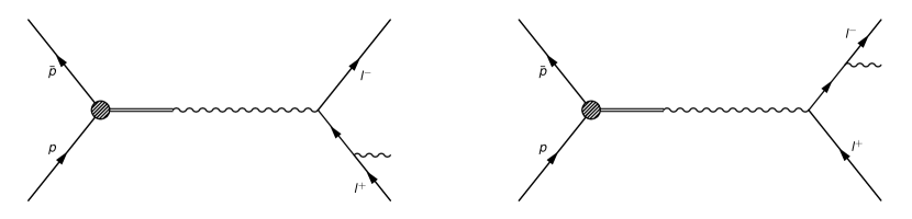
Figure 1: Diagrams for decay $X\longrightarrow\gamma l^{+}l^{-}$.

In Figure 1, we present the diagrams for the decay $X\longrightarrow\gamma l^{+}l^{-}$. Since $m_{X}\ll m_{Z},m_{H}$ (where $m_{Z}$ and $m_{H}$ represent the masses of the Z boson and the Higgs boson, respectively), we only consider the Feynman diagrams where the photon serves as the intermediate line for the decay $X\longrightarrow\gamma l^{+}l^{-}$. Additionally, due to charge-conjugation invariance FermilabE760:1996jsx , the photon in the final state can only be emitted by one of the charged leptons in the final state. Therefore, we consider the diagrams shown in Figure 1. Direct calculation yields the following result:

$$\sum_{\lambda_{Q},\lambda_{\bar{Q}}=\pm 1}\left|\mathcal{M}(\vec{0},\vec{0}\rightarrow\gamma l^{+}l^{-})\right|^{2}=-\frac{4096\pi^{3}\mathcal{Q}_{Q}^{2}\alpha^{3}}{m_{X}^{4}\left(m_{X}-2\sqrt{p^{2}_{l^{-}}+m_{l}^{2}}\right)^{2}\left(m_{X}-2\left(\sqrt{p^{2}_{l^{-}}+m_{l}^{2}}+{E_{\gamma}}\right)\right)^{2}}\times$$

$$\left(2p^{2}_{l^{-}}m_{X}\left(m_{X}\left(-8m_{X}\sqrt{p^{2}_{l^{-}}+m_{l}^{2}}+8{E_{\gamma}}\sqrt{p^{2}_{l^{-}}+m_{l}^{2}}+7m_{X}^{2}-14m_{X}{E_{\gamma}}+6{E^{2}_{\gamma}}\right)+2m_{l}^{2}(5m_{X}-2{E_{\gamma}})\right)\right.$$

$$~{}~{}+m_{X}^{2}(m_{X}-{E_{\gamma}})\left(-3m_{X}^{2}\left(2\sqrt{p^{2}_{l^{-}}+m_{l}^{2}}+{E_{\gamma}}\right)+2m_{X}{E_{\gamma}}\left(6\sqrt{p^{2}_{l^{-}}+m_{l}^{2}}+{E_{\gamma}}\right)-4{E^{2}_{\gamma}}\sqrt{p^{2}_{l^{-}}+m_{l}^{2}}+m_{X}^{3}\right)$$

$$~{}~{}+4m_{l}^{4}\left(3m_{X}^{2}-2m_{X}{E_{\gamma}}+{E^{2}_{\gamma}}\right)+8p^{4}_{l^{-}}m_{X}^{2}$$

$$~{}~{}+m_{l}^{2}m_{X}\left.\left(-4m_{X}^{2}\left(5\sqrt{p^{2}_{l^{-}}+m_{l}^{2}}+8{E_{\gamma}}\right)+2m_{X}{E_{\gamma}}\left(14\sqrt{p^{2}_{l^{-}}+m_{l}^{2}}+9{E_{\gamma}}\right)-8{E^{2}_{\gamma}}\sqrt{p^{2}_{l^{-}}+m_{l}^{2}}+15m_{X}^{3}\right)\right)~{},$$ (17)

where $\mathcal{Q}_{Q/\bar{Q}}$ and $\lambda_{Q/\bar{Q}}$ represent the electric charge and helicity of the $Q/\bar{Q}$ from the quarkonia $X$, respectively. According to experimental results, only the squared amplitude with $\lambda_{Q}=-\lambda_{\bar{Q}}$ contributes to the decay of $J/\Psi$. Based on numerical integration results, we find the relationship

$$\int d\Pi_{f}\left|\mathcal{M}(\vec{0},\vec{0};\lambda_{Q}=\lambda_{\bar{Q}}\rightarrow\gamma l^{+}l^{-})\right|^{2}\approx\frac{1}{2}\int d\Pi_{f}\left|\mathcal{M}(\vec{0},\vec{0};\lambda_{Q}=-\lambda_{\bar{Q}}\rightarrow\gamma l^{+}l^{-})\right|^{2}~{}.$$ (18)

It should be noted that the relative difference between the left-hand and right-hand sides of Eq. (18) is approximately $10^{-4}$ according to numerical results.

As an example, let us consider the decay $J/\Psi\to\gamma\mu^{+}\mu^{-}$. By considering the squared amplitude with $\lambda_{c}=-\lambda_{\bar{c}}$ and the phase space in the rest frame of $J/\Psi$, numerical integration yields the angular and energy/momentum distributions of the final state particles, as shown in Figure 2 with $E_{\gamma\text{cut}}=0.025,~{}0.1$ GeV and in Figure 3 with $E_{\gamma\text{cut}}=0.1$ GeV. From the lowest panel of Figure 2, it can be observed that the radiative photons tend to move along the collinear ($\theta_{\gamma\mu^{-}}=0$) and opposite ($\theta_{\gamma\mu^{-}}=\pi$) directions of $\mu^{-}$ motion due to the collinear singularity.

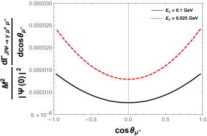
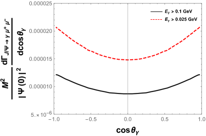
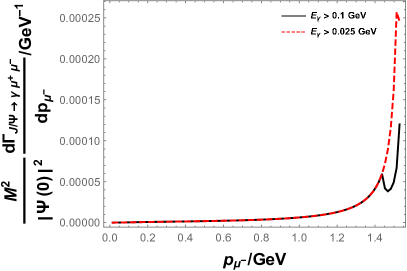
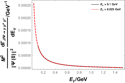
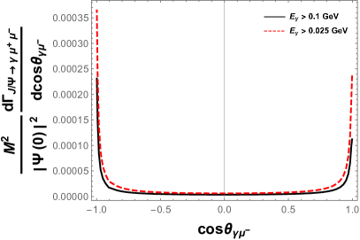
Figure 2: Angular and energy/momentum distributions of $\gamma$ and $\mu^{-}$ from the decay $J/\Psi\to\gamma\mu^{+}\mu^{-}$ in the $J/\Psi$ rest frame. $\theta_{\gamma}$, $\theta_{\mu^{-}}$, and $\theta_{\gamma\mu^{-}}$ are polar angles of $\gamma$ and $\mu^{-}$, and the angle between the moving directions of $\gamma$ and $\mu^{-}$, respectively. $E_{\gamma}$ and $p_{\mu^{-}}$ are the photon energy and $\mu^{-}$ momentum, respectively. Two kinds of photon energy cut are chosen.

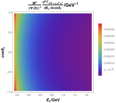
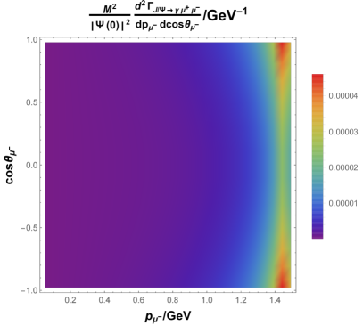
Figure 3: Left panel: polar angle-energy distribution of $\gamma$ from the decay $J/\Psi\to\gamma\mu^{+}\mu^{-}$ in the $J/\Psi$ rest frame at $E_{\gamma\text{cut}}=0.1$ GeV. Right panel: polar angle-momentum distribution of $\mu^{-}$ from the decay $J/\Psi\to\gamma\mu^{+}\mu^{-}$ in the $J/\Psi$ rest frame at $E_{\gamma\text{cut}}=0.1$ GeV.

4 Expression of ${\Gamma_{X\rightarrow\gamma l^{+}l^{-}}}$ derived in the $l^{+}l^{-}$ c.m. frame

Although the final states consist of three particles ($l^{+}$, $l^{-}$, and $\gamma$), it is advantageous to analyze the decay of $X$ in the c.m. frame of the $l^{+}l^{-}$ system. In this frame, we can employ a set of variables to describe the angular distributions of the photon and leptons, as well as their relative motion. Specifically, we introduce $\Omega_{\gamma}^{\prime}$ ($\theta_{\gamma}^{\prime}$ and $\phi_{\gamma}^{\prime}$) and $\Omega_{l}^{\prime}$ ($\theta_{l}^{\prime}$ and $\phi_{l}^{\prime}$) to represent the angles of the photon and leptons, respectively, in the $l^{+}l^{-}$ c.m. frame. Furthermore, we use $\theta^{\prime}_{\gamma l}$ to denote the angle between the directions of motions of the photon and the lepton in this frame. To quantify the kinematics, we introduce $\beta^{\prime}$, $E_{\gamma}^{\prime}$, and $s^{\prime}$ to represent the velocity of the leptons, the energy of the photon, and the square of the invariant mass of the $l^{+}l^{-}$ system, respectively. By using the given quantities, we can parameterize the four-momentum of the final states in the c.m. frame of $l^{+}l^{-}$ as follows:

$$p_{l^{-}}^{\prime\mu}=(\sqrt{s^{\prime}}/{2},~{}0,~{}0,~{}\sqrt{{s^{\prime}}/{4}-m_{l}^{2}})~{},$$ (19)

$$p_{l^{+}}^{\prime\mu}=(\sqrt{s^{\prime}}/{2},~{}0,~{}0,~{}-\sqrt{{s^{\prime}}/{4}-m_{l}^{2}})~{},$$ (20)

$$p_{\gamma}^{\prime\mu}=(E_{\gamma}^{\prime},~{}E_{\gamma}^{\prime}\sin\theta^{\prime}_{\gamma l}\cos\phi_{\gamma}^{\prime},~{}E_{\gamma}^{\prime}\sin\theta^{\prime}_{\gamma l}\sin\phi_{\gamma}^{\prime},~{}E_{\gamma}^{\prime}\cos\theta^{\prime}_{\gamma l})~{},$$ (21)

where we have chosen the direction of motion of $l^{-}$ as the z-axis direction, resulting in $\theta_{\gamma}^{\prime}=\theta^{\prime}_{\gamma l}$. Using the relation $p^{\prime 2}_{X}=(p_{l^{-}}^{\prime}+p_{l^{+}}^{\prime}+p_{\gamma}^{\prime})^{2}=m_{X}^{2}$, we find

$$s^{\prime}=\left(\sqrt{m_{X}^{2}+E_{\gamma}^{\prime 2}}-E_{\gamma}^{\prime}\right)^{2}~{},$$ (22)

$$\beta^{\prime}=\sqrt{1-\frac{4m_{l}^{2}}{\left(\sqrt{m_{X}^{2}+E_{\gamma}^{\prime 2}}-E_{\gamma}^{\prime}\right)^{2}}}~{}.$$ (23)

To ensure $s^{\prime}>4m_{l}^{2}$, we obtain the upper limit for $E_{\gamma}^{\prime}$ as

$$E_{\gamma}^{\prime}<\frac{m_{X}^{2}}{4m_{l}}-m_{l}~{}.$$ (24)

The photon energy cut $E_{\gamma\text{cut}}$ in the $X$ rest frame corresponds to the lower limit $E^{\prime}_{\gamma\text{cut}}$ for $E_{\gamma}^{\prime}$ in the $l^{+}l^{-}$ c.m. frame, given by

$$E^{\prime}_{\gamma\text{cut}}=E_{\gamma\text{cut}}\sqrt{\frac{1}{1-2\frac{E_{\gamma\text{cut}}}{m_{X}}}}<E_{\gamma}^{\prime}~{}.$$ (25)

The parameter of the Lorentz transformation from the $X$ rest frame to the $l^{+}l^{-}$ c.m. frame is given by

$$\vec{\beta}=-\frac{\vec{p}^{\prime}_{\gamma}}{\sqrt{m_{X}^{2}+E_{\gamma}^{\prime 2}}}~{},$$ (26)

where $\vec{p}^{\prime}_{\gamma}$ is the three-momentum of the photon in the $l^{+}l^{-}$ c.m. frame. Thus, the $l^{+}l^{-}$ c.m. frame changes with the photon energy and angles, and we need to determine the Jacobi factor $J$ appearing in the following equation:

$$\frac{d^{3}\vec{p}_{l^{-}}}{(2\pi)^{3}2E_{l^{-}}}\frac{d^{3}\vec{p}_{l^{+}}}{(2\pi)^{3}2E_{l^{+}}}\frac{d^{3}\vec{p}_{\gamma}}{(2\pi)^{3}2E_{\gamma}}(2\pi)^{4}\delta^{4}(p^{\mu}_{X}-p^{\mu}_{l^{-}}-p^{\mu}_{l^{+}}-p^{\mu}_{\gamma})$$

$$= J\times\frac{d^{3}\vec{p}^{\prime}_{l^{-}}}{(2\pi)^{3}2E^{\prime}_{l^{-}}}\frac{d^{3}\vec{p}^{\prime}_{l^{+}}}{(2\pi)^{3}2E^{\prime}_{l^{+}}}\frac{d^{3}\vec{p}^{\prime}_{\gamma}}{(2\pi)^{3}2E^{\prime}_{\gamma}}(2\pi)^{4}\delta^{4}(p^{\prime\mu}_{X}-p^{\prime\mu}_{l^{-}}-p^{\prime\mu}_{l^{+}}-p^{\prime\mu}_{\gamma})~{},$$ (27)

where $\vec{p}_{l^{-}}$, $\vec{p}_{l^{+}}$, and $\vec{p}_{\gamma}$ ($\vec{p}^{\prime}_{l^{-}}$, $\vec{p}^{\prime}_{l^{+}}$, and $\vec{p}^{\prime}_{\gamma}$) are the three-momenta of $l^{-}$, $l^{+}$, and $\gamma$ in the $X$ rest frame ($l^{+}l^{-}$ c.m. frame), respectively. Direct derivations demonstrate that the Jacobi factor $J$ is related to the partial derivatives of the four-momentum of $l^{-}$ and $\gamma$ in the $X$ rest frame with respect to those in the $l^{+}l^{-}$ c.m. frame, giving us

$$J=J(p^{\mu}_{l^{-}},p^{\mu}_{\gamma};p^{\prime\mu}_{l^{-}},p^{\prime\mu}_{\gamma})=J(E_{\gamma}^{\prime})=1+\frac{E^{\prime 2}_{\gamma}}{m_{X}^{2}}\left(4-\frac{E^{\prime}_{\gamma}}{\sqrt{m_{X}^{2}+E^{\prime 2}_{\gamma}}}-3\frac{\sqrt{m_{X}^{2}+E^{\prime 2}_{\gamma}}}{E^{\prime}_{\gamma}}\right)~{}.$$ (28)

Therefore, we have

$$J(E_{\gamma}^{\prime}\ll m_{X})=1~{},$$ (29)

$$J(E_{\gamma}^{\prime}\gg m_{X})=0~{},$$ (30)

which indicates that the production of high-energy photons in the $l^{+}l^{-}$ c.m. frame is suppressed.

According to Eq. (15), the decay width of quarkonia $X$ decaying into specific final states is directly proportional to the squared amplitude of the wave function at the origin, represented as $|\psi(\vec{0})|^{2}$. Consequently, the ratio between the decay widths of different decay modes of $X$ is independent of the specific value of $|\psi(\vec{0})|^{2}$. By taking into account the phase space, the Jacobi factor resulting from the Lorentz transformation, the squared amplitude in the center-of-mass frame of the $l^{+}l^{-}$ pair, and integrating over the final state angles, we derive the following expression:

$$\frac{\Gamma_{X\rightarrow\gamma l^{+}l^{-}}}{\Gamma_{X\rightarrow l^{+}l^{-}}}= {\frac{8\alpha b}{{\pi(1+2b)\sqrt{1-4b}}}}\int_{0}^{\sqrt{1-\frac{4b}{(\sqrt{1+c^{2}}-c)^{2}}}}d\beta^{\prime}\frac{\beta^{\prime}}{(1-\beta^{\prime 2})\left(1-\beta^{\prime 2}-4b\right)}$$

$$\times\left(-\beta^{\prime}{\left(1+b^{2}\frac{16(2-\beta^{\prime 2})}{(1-\beta^{\prime 2})^{2}}\right)}+{\left((1-4b)+b^{2}\frac{8(3-\beta^{\prime 4})}{(1-\beta^{\prime 2})^{2}}\right)}\ln\left[\frac{1+\beta^{\prime}}{1-\beta^{\prime}}\right]\right)\equiv g^{\prime}(b,c)~{},$$ (31)

where

$$b=\frac{m_{l}^{2}}{m_{X}^{2}}~{},$$ (32)

$$c=\frac{E_{\gamma\text{cut}}}{m_{X}}\sqrt{\frac{1}{1-2\frac{E_{\gamma\text{cut}}}{m_{X}}}}~{}.$$ (33)

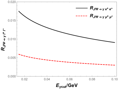
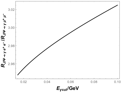
Figure 4: Left panel: branching ratios of $J/\Psi\to\gamma e^{+}e^{-}$ and $J/\Psi\to\gamma\mu^{+}\mu^{-}$ at different $E_{\gamma\text{cut}}$. The ratio between $R_{J/\Psi\to\gamma e^{+}e^{-}}$ and $R_{J/\Psi\to\gamma\mu^{+}\mu^{-}}$ at different $E_{\gamma\text{cut}}$.

Utilizing the experimentally measured values of $R_{J/\Psi\to e^{+}e^{-}}=(5.971\pm 0.032)\%$ and $R_{J/\Psi\to\mu^{+}\mu^{-}}=(5.961\pm 0.033)\%$ obtained from the PDG ParticleDataGroup:2022pth , and employing the ratio ${\Gamma_{X\rightarrow\gamma l^{+}l^{-}}}/{\Gamma_{X\rightarrow l^{+}l^{-}}}$ derived from Eq. (31), we can calculate the branching ratios of $J/\Psi\to\gamma e^{+}e^{-}$ and $J/\Psi\to\gamma\mu^{+}\mu^{-}$ at various $E_{\gamma\text{cut}}$ values, as depicted in Figure 4. Notably, it is noteworthy that the ratio between $R_{J/\Psi\to\gamma e^{+}e^{-}}$ and $R_{J/\Psi\to\gamma\mu^{+}\mu^{-}}$ consistently remains around 3.0 within the range of $E_{\gamma\text{cut}}$ spanning from $\mathcal{O}(0.01)$ to $\mathcal{O}(0.1)$ GeV. The future experimental results of this ratio will serve as a direct test of lepton flavor universality (LFU).

In Ref. FermilabE760:1996jsx , the differential decay width for the process $X\rightarrow\gamma l^{+}l^{-}$ is given by

$$d\Gamma_{X\rightarrow\gamma l^{+}l^{-}}=d\Gamma_{X\rightarrow l^{+}l^{-}}\beta^{\prime 3}\frac{2\alpha}{\pi}\frac{dE_{\gamma}^{\prime}}{E_{\gamma}^{\prime}}\frac{s^{\prime}}{m_{X}^{2}}\frac{1-\cos^{2}\theta_{\gamma l}^{\prime}}{\left(1-\beta^{\prime 2}\cos^{2}\theta_{\gamma l}^{\prime}\right)^{2}}d\Omega_{\gamma}^{\prime}~{},$$ (34)

where

$$d\Gamma_{X\rightarrow l^{+}l^{-}}=\frac{3}{3+\lambda}\left(1+\lambda\cos^{2}\theta_{l}^{\prime}\right)\Gamma_{X\rightarrow l^{+}l^{-}}\frac{d\Omega_{l}^{\prime}}{4\pi}~{}.$$ (35)

Upon integrating out the final state angles ($\Omega^{\prime}_{\gamma}$ and $\Omega^{\prime}_{l}$), we obtain the ratio of the decay widths as

$$\frac{\Gamma_{X\rightarrow\gamma l^{+}l^{-}}}{\Gamma_{X\rightarrow l^{+}l^{-}}}= 16\alpha b\int_{0}^{\sqrt{1-\frac{4b}{(\sqrt{1+c^{2}}-c)^{2}}}}d\beta^{\prime}{\frac{\beta^{\prime}}{(1-\beta^{\prime 2})\left(1-\beta^{\prime 2}-4b\right)}}$$

$$\times{\left(-\beta^{\prime}{\left(1+b\frac{4}{1-\beta^{\prime 2}}\right)}+{\left(1+b\frac{4}{1-\beta^{\prime 2}}\right)\frac{1+\beta^{\prime 2}}{2}}\ln\left[\frac{1+\beta^{\prime}}{1-\beta^{\prime}}\right]\right)}\equiv g(b,c)~{}.$$ (36)

While there exists an analytical result for the integration in Eq. (36), we refrain from presenting it here due to its tedious and easily obtainable nature.

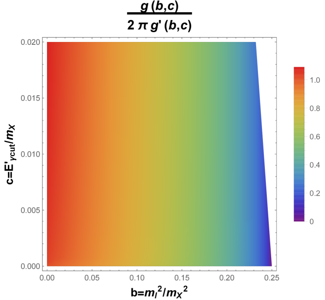
Figure 5: The ratio between the predicted values of ${\Gamma_{X\rightarrow\gamma l^{+}l^{-}}}/{\Gamma_{X\rightarrow l^{+}l^{-}}}$ using $\frac{g(c,b)}{2\pi}$ and $g^{\prime}(b,c)$.

The comparison between $g(b,c)$ derived from the relation proposed in Ref. FermilabE760:1996jsx and $g^{\prime}(b,c)$ obtained in this study reveals differences arising from the prefactors and integrated functions of $\beta^{\prime}$.

The dependencies of $\frac{g(b,c)}{2\pi g^{\prime}(b,c)}$ on $b$ and $c$ are illustrated in Figure 5. It is observed that the ratio $\frac{g(b,c)}{2\pi g^{\prime}(b,c)}$ is greater than one for small values of $b$ (e.g., $b<0.03$ when $c=0.02$) and decreases as $b$ increases.

In the specific case where $E_{\gamma\text{cut}}=0.1$ GeV and $X$ includes $J/\Psi$, $\Psi(2S)$, $\Upsilon(1S)$, and $\Upsilon(2S)$, the ratio between ${\Gamma_{X\rightarrow\gamma l^{+}l^{-}}}$ and ${\Gamma_{X\rightarrow l^{+}l^{-}}}$, as determined by $g(b,c)$ and $g^{\prime}(b,c)$, is presented in Table 1. It is found that for modes with $b$ approximately equal to or smaller than $\mathcal{O}(10^{-2})$, $\frac{g(c,b)}{2\pi}$, rather than $g(c,b)$, is comparable to $g^{\prime}(c,b)$, with a relative difference within 10%. The largest discrepancy between $\frac{g(c,b)}{2\pi}$ and $g^{\prime}(c,b)$ is observed for the mode ${{\Psi(2S)\rightarrow(\gamma)\tau^{+}\tau^{-}}}$, where $b=0.232$, and $g^{\prime}(c,b)$ is four times larger than $\frac{g(c,b)}{2\pi}$. Compared to $\frac{g(c,b)}{2\pi}$, the factor $\frac{1}{(1+2b)\sqrt{1-4b}}$ in $g^{\prime}(c,b)$ yields a 2.5-fold enhancement for the decay mode ${{\Psi(2S)\rightarrow(\gamma)\tau^{+}\tau^{-}}}$ when $b=0.232$. By disregarding the differences in the prefactors between $\frac{g(c,b)}{2\pi}$ and $g^{\prime}(c,b)$, which are negligible when $b\ll 1$, the remaining enhancement in $g^{\prime}(c,b)$ for the ${{\Psi(2S)\rightarrow(\gamma)\tau^{+}\tau^{-}}}$ decay mode can be attributed to the variations in the integrated functions.

Mode	$b$	$c$ ($E_{\gamma\text{cut}}=0.1$ GeV)	$g^{\prime}(c,b)$	$\frac{g(c,b)}{2\pi g^{\prime}(c,b)}$
${{J/\Psi\rightarrow(\gamma)e^{+}e^{-}}}$	$2.72\times 10^{-8}$	$3.34\times 10^{-2}$	0.152	1.11
${{J/\Psi\rightarrow(\gamma)\mu^{+}\mu^{-}}}$	$1.16\times 10^{-3}$	$3.34\times 10^{-2}$	$5.04\times 10^{-2}$	1.10
${{\Psi(2S)\rightarrow(\gamma)e^{+}e^{-}}}$	$1.92\times 10^{-8}$	$2.79\times 10^{-2}$	0.168	1.10
${{\Psi(2S)\rightarrow(\gamma)\mu^{+}\mu^{-}}}$	$8.22\times 10^{-4}$	$2.79\times 10^{-2}$	$5.84\times 10^{-2}$	1.10
${{\Psi(2S)\rightarrow(\gamma)\tau^{+}\tau^{-}}}$	0.232	$2.79\times 10^{-2}$	$6.09\times 10^{-6}$	0.25
${{\Upsilon(1S)\rightarrow(\gamma)e^{+}e^{-}}}$	$2.92\times 10^{-9}$	$1.07\times 10^{-2}$	0.266	1.08
${{\Upsilon(1S)\rightarrow(\gamma)\mu^{+}\mu^{-}}}$	$1.25\times 10^{-4}$	$1.07\times 10^{-2}$	0.111	1.07
${{\Upsilon(1S)\rightarrow(\gamma)\tau^{+}\tau^{-}}}$	$3.53\times 10^{-2}$	$1.07\times 10^{-2}$	$2.80\times 10^{-2}$	0.98
${{\Upsilon(2S)\rightarrow(\gamma)e^{+}e^{-}}}$	$2.60\times 10^{-9}$	$1.01\times 10^{-2}$	0.273	1.07
${{\Upsilon(2S)\rightarrow(\gamma)\mu^{+}\mu^{-}}}$	$1.11\times 10^{-4}$	$1.01\times 10^{-2}$	0.115	1.07
${{\Upsilon(2S)\rightarrow(\gamma)\tau^{+}\tau^{-}}}$	$3.14\times 10^{-2}$	$1.01\times 10^{-2}$	$3.04\times 10^{-2}$	0.99

Table 1: ${\Gamma_{X\rightarrow\gamma l^{+}l^{-}}}/{\Gamma_{X\rightarrow l^{+}l^{-}}}$ determined by $g^{\prime}(b,c)$ and the ratio between the predicted values of ${\Gamma_{X\rightarrow\gamma l^{+}l^{-}}}/{\Gamma_{X\rightarrow l^{+}l^{-}}}$ using $\frac{g(c,b)}{2\pi}$ and $g^{\prime}(b,c)$. $X$ represents $J/\Psi$, $\Psi(2S)$, $\Upsilon(1S)$, and $\Upsilon(2S)$.

5 Conclusion

This study focuses on the leptonic decays of heavy quarkonia $X$, which is considered as bound state of a quark ($Q$) and an antiquark ($\bar{Q}$) with zero momentum. By analyzing the squared amplitude of the decay $X\to\gamma l^{+}l^{-}$ and studying the kinematics of the final states in the rest frame of $X$, we calculate the decay widths and branching ratios of the three-body leptonic decays of $X$. Furthermore, the angular and energy/momentum distributions of the final state particles in the $X$ rest frame are determined through numerical integration.

To investigate the Lorentz transformation from the $X$ rest frame to the c.m. frame of $l^{+}l^{-}$, we derive the Jacobi factor of this transformation and the phase space in the $l^{+}l^{-}$ c.m. frame. Based on these considerations, we provide a prediction of the ratio between ${\Gamma_{X\rightarrow\gamma l^{+}l^{-}}}$ and ${\Gamma_{X\rightarrow l^{+}l^{-}}}$. However, our proposed expression differs from the one presented in Ref. FermilabE760:1996jsx , and the relative difference becomes significant when $m_{l}^{2}/m_{X}^{2}$ exceeds a threshold of approximately $\mathcal{O}(0.1)$.

We examine the predicted ratios for different heavy quarkonia, including $J/\Psi$, $\Psi(2S)$, $\Upsilon(1S)$, and $\Upsilon(2S)$. Our results show that the ratios obtained from the proposed relation are in good agreement with those derived from the literature (divided by $2\pi$), with relative differences typically around or below 10%. However, an exception arises for the ratio between ${\Gamma_{\Psi(2S)\to\gamma\tau^{+}\tau^{-}}}$ and ${\Gamma_{\Psi(2S)\to\tau^{+}\tau^{-}}}$, where the prediction from the proposed expression is four times larger. It is worth noting that the results obtained in this study can be directly compared to future measurements at BESIII, B factory experiments and others.

References

(1)
E. Barberio, B. van Eijk, and Z. Was, Comput. Phys. Commun.66
(1991)
115.
(2)
E. Barberio and Z. Was, Comput. Phys. Commun.79 (1994)
291–308.