Experimental simulation of quantum superchannels

Abstract

Simulating quantum physical processes has been one of the major motivations for quantum information science. Quantum channels, which are completely positive and trace preserving processes, are the standard mathematical language to describe quantum evolution, while in recent years quantum superchannels have emerged as the substantial extension. Superchannels capture effects of quantum memory and non-Markovianality more precisely, and have found broad applications in universal models, algorithm, metrology, discrimination tasks, as examples. Here, we report an experimental simulation of qubit superchannels in a nuclear magnetic resonance (NMR) system with high accuracy, based on a recently developed quantum algorithm for superchannel simulation. Our algorithm applies to arbitrary target superchannels, and our experiment shows the high quality of NMR simulators for near-term usage. Our approach can also be adapted to other experimental systems and demonstrates prospects for more applications of superchannels.

I Introduction

Quantum simulation is one of the original motivations for quantum computing Fey82. Although being noisy without the aid of quantum error correction NC00, experimental quantum simulation is valuable for verifying quantum algorithms and protocols, for developing new quantum information-processing techniques, and even for the exploration of quantum advantage Pre18. General quantum evolution is described as completely positive mappings CHOI1975285, which can describe both unitary and non-unitary processes, including measurements. Studying non-unitary dissipative processes are important to understand the physics of decoherence Bre03, quantum error correction NC00, and so on. In recent years, quantum simulation of channels, including open-system dynamics, have been studied both theoretically and experimentally BBW07; PPK+11; WBOS13; WS15; Wang16; SSP14; SSBP15; TV17; TFS+16; CMP+18; LLW+17; XWP+17; MMR18; LXW+18; PJO+20; GRM20.

Similar to quantum channels CHOI1975285 which describe the relationship of input-output states for a quantum system, quantum superchannels CDP08a; CDP08; CDP09, also known as supermaps or combs, describe the relationships between input and output quantum channels. Although a superchannel can also be treated as a channel, it captures some peculiar features more precisely, such as quantum non-Markovianality LHW18 and quantum resources RevModPhys.91.025001. In recent years, superchannel theory has been widely used for studying channel discrimination and quantum metrology CAP08; 8678741, ebit-assisted quantum communication and error correction LB12, a computing model without definite causal order CAPV13, quantum von Neumann architecture W20_choi; Wang_2022; LWLW23 and quantum algorithms like quantum machine learning and quantum optimization VPB18; MBW+19; HKP21; W21_model.

Experimental quantum simulation is indispensable for some applications especially when the simulated target is hard to obtain. Nuclear magnetic resonance (NMR) has been well developed as a sophisticated technology in recent decades for quantum information processing NC00; MLSK02; VC05; Xin_2018. Different from other platforms LJL+10, liquid-state NMR quantum simulators realize entangling operations on the so-called pseudo-pure states and benefit from its computer-aided high-fidelity pulse-engineering technology and controlling in full range of the system dynamics. Although being limited on qubit numbers and sampling cost, which are similar with some NISQ (noisy intermediate-scale quantum) tasks Pre18, NMR quantum simulators are able to simulate quantum systems of small-to-medium sizes with complex or time-dependent Hamiltonian and test new protocols, such as open-system dynamics XWP+17, quantum phase transition peng2009quantum, gate characterization lu2015experimental, measuring correlation functions li2017measuring, quantum imaginary evolution cao2022quantum, heat conduction wei2023quantum and quantum energy teleportation RKM+23.

In this work, we implement quantum superchannels based on a recent simulation algorithm WW23. A central part of the algorithm is the decomposition into a convex sum of generalized extreme superchannels, which not only benefits practical simulation, but also is relevant for the study of information-theoretic features of channels and superchannels, e.g., for quantum channel capacity Smi08. Our theory applies to arbitrary form of superchannels, and it employs a convex-sum decomposition to reduce the circuit simulation cost. A unitary circuit that simulates a channel or superchannel is further converted to a Hamiltonian evolution for the NMR experimental simulation. Our 4-qubit NMR simulator, assisted by the simulation algorithm, is able to realize any qubit superchannel with high fidelity (see Fig. 1). Its circuit contains a pair of pre- and post-unitary operators on the input channel with ancillary qubits serving as quantum memory. We experimentally carried out a few tasks, including randomly generating so-called extreme superchannels, a convex-decomposition of random non-extreme superchannels, and also random dephasing superchannels. Our experiment can also be viewed as a first step to confirm the feasibility of the recent construction of prototypes of quantum von Neumann architecture LWLW23 which has a close relation with superchannels. We also theoretically demonstrate the application of superchannels for noise-adapted quantum error correction of the amplitude damping channel in the appendix B.

The remainder of our paper is organised as follows. Section II introduces the algorithm we use simulating superchannels. Section III presents the experimental method and results. We summarise our paper in Section IV. Further numerical details are reported in the Appendix A and some other examples of superchannel in Appendix B.

II The algorithm

Our goal is to experimentally simulate arbitrary superchannels within a good accuracy. Usually, quantum evolutions are in general described by completely positive trace-preserving (CPTP) maps, also known as quantum channels NC00

$$\mathcal{E}(\rho)=\sum_{i=1}^{r}K_{i}\rho K_{i}^{\dagger},\,\rho\in\mathcal{D}(\mathscr{H}),\,\sum_{i}K_{i}^{\dagger}K_{i}=\mathds{1}$$ (1)

for $\{K_{i}\}$ the Kraus operators Kra83. As an example, a unitary ‘qudit’ evolution $U\rho U^{\dagger}$, $U\in SU(d)$ WHSK20 satisfies $U^{\dagger}U=UU^{\dagger}=\mathds{1}$, with $d=\text{dim}(\mathscr{H})$.

Channel-state duality Jam72; CHOI1975285 maps a channel $\mathcal{E}\in\mathscr{L}(\mathscr{D})$ into a Choi state

$$\omega_{\mathcal{E}}:=(\mathcal{E}\otimes\mathds{1})(|\omega\rangle\langle\omega|),$$ (2)

with $|\omega\rangle:=\frac{1}{\sqrt{d}}\sum_{i=0}^{d-1}|i,i\rangle$ a maximally entangled state, also known as a (generalised) Bell state. The rank of the Choi state equals the rank of the channel, which is the minimal number of Kraus operators.

As channels can be viewed as states, the operations on them are further defined as superchannels CDP08a; CDP08; CDP09. Similar with channels, superchannels can also be well represented by quantum circuits, Kraus operators, and also Choi states. Given a channel with a set of Kraus operators $\mathcal{E}=\{K_{i}\}$ and Choi state $\omega_{\mathcal{E}}$, it is changed by a superchannel $\hat{\mathcal{S}}$ according to

$$\hat{\mathcal{S}}(\omega_{\mathcal{E}})=\sum_{a}S_{a}\omega_{\mathcal{E}}S_{a}^{\dagger}$$ (3)

with

$$S_{a}=\sum_{m}K_{w}^{ma}\otimes K_{v}^{m}$$ (4)

and $\sum_{a}S_{a}^{\dagger}S_{a}=\mathds{1}$ for trace preserving. We place a hat on the symbol for superchannels to avoid confusion. Subscripts $v$ and $w$ (4) are pre- and post-unitary operators on channels. Kraus operators of the output channel are represented as

$$F_{i}^{a}=\sum_{m}K_{w}^{ma}K_{i}K_{v}^{m,t},$$ (5)

with $K_{v}^{m}=\bra{m}V\ket{0}$, $K_{w}^{ma}=\bra{m}W\ket{a}$, and $t$ stands for transposition.

Given an arbitrary superchannel, an algorithm has been developed recently for the task of circuit simulation of the superchannel WW23. The algorithm also explores the convexity of the set of superchannels. Being convex, there are extreme points that cannot be written as any convex combination of others bengtsson_zyczkowski_2006. Choi proved that a channel $\mathcal{E}$ is extreme iff $\{K_{i}^{\dagger}K_{j}\}$ is linearly independent CHOI1975285, which has been extended to superchannels DPS11. This yields an upper bound on the rank which is a necessary condition, leading to the notion of generalized extreme points Rus07, or gen-extreme points W20_choi. Previous studies Rus07; WBOS13; WS15; Wang16; W20_choi; WW23 shows that decomposition via convex combination of gen-extreme points is a viable approach. In this work, we adapt this algorithm to our NMR simulator to realize arbitrary qubit superchannels to high accuracy.

The circuit form of a qubit gen-extreme superchannel is shown in Fig.1. It contains 4 qubits and 3 steps for the evolution: a pre- and post-unitary operation, and the input channel in the middle. The top register is the ancilla to realize any qubit channel, and it is proven that a single qubit is enough RSW02; WBOS13. The 2nd register is the qubit system, and the remaining two are the ancilla to realize the superchannel. A direct application of Stinespring dilation would require 3 more qubits, hence a lot more gates, with one (two) for the channel (superchannel), which can be easily verified from their ranks.

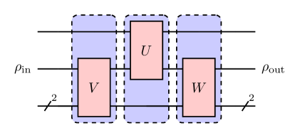
Figure 1: Circuit form of a qubit gen-extreme superchannel

Our algorithm $\mathcal{A}$ accepts an arbitrary target superchannel $\hat{\mathcal{S}}$ as the input, in the form of its Choi state $\omega_{\hat{\mathcal{S}}}$, for instance, and uses an optimization scheme from a built-in package of MATLAB WW23 to minimize the trace distance $d(\omega_{\hat{\mathcal{S}}},\omega_{\hat{\mathcal{S}}^{\prime}})$. This trace distance represents simulation accuracy for

$$\hat{\mathcal{S}}^{\prime}=\sum_{i=1}^{4}p_{i}\hat{\mathcal{S}}^{g}_{i},$$ (6)

which is a convex combination of gen-extreme superchannels with $p_{i}$ as a probability and $\hat{\mathcal{S}}^{g}_{i}$ as a gen-extreme superchannel. Our numerical simulation can guarantee the accuracy in the order of $10^{-3}$ to $10^{-4}$ WW23. A gen-extreme superchannel is parameterized based on the cosine-sine decomposition of unitary operator Wang16.

To implement a unitary circuit $U$, the NMR system encodes a qubit as the nuclear spin states, and converts $U$ into a Hamiltonian evolution $\text{e}^{-\text{i}tH}$, which are realized by a sequence of so-called control pulses which manipulates the interaction among nuclear spins. It does not directly decompose $U$ as a sequence of elementary gates, such as Hadamard and controlled-NOT NC00, and then implement each gate approximately which may result in a quick accumulation of errors. Instead, it employs algorithms to design control pulses as an engineered Hamiltonian evolution. Namely, the gradient ascent pulse-engineering (GRAPE) technique khaneja2005optimal; ryan2008liquid is used to design the pulse sequence and achieve the optimal control of radio-frequency field of NMR spectrometer. For a given unitary operation $U$, the principle of GRAPE is to calculate the gradient of the fitness function corresponding to the forward and backward unitary propagators, and the obtained gradient indicates the direction that the control pulses should be optimized to improve the fitness function. In general, the GRAPE algorithm is implemented fully on a classical computer.

To verify the quality of experimental simulation, we perform quantum process tomography NC00 for randomly chosen input channel $\mathcal{E}$ and output channel $\hat{\mathcal{S}}(\mathcal{E})$ from a superchannel $\hat{\mathcal{S}}$. We shall note that for arbitrary random superchannels, our algorithm above only works effectively for small dimensions as the number of parameters for a superchannel scales exponentially with the physical system size. However, we leave it for further study of efficient simulation for special types of channels and superchannels of higher dimensions.

This completes the description of our algorithm. In the next section, we present the details for the implementation of a few simulation tasks: random gen-extreme superchannel, random dephasing superchannel, and also a demonstration of the convex decomposition method.

III Experimental simulation

Several superchannels are demonstrated experimentally in the NMR system. We firstly achieve a random gen-extreme superchannel in experiment, displaying the accuracy of superchannel simulation in the NMR system. Then we achieve a dephasing superchannel PKS+21, which is the analog of dephasing channels NC00 that only affect phase information without the loss of energy. Finally, we demonstrate the decomposition of a random superchannel, showing a great agreement with the theory WW23.

All experiments are conducted in a liquid NMR system, where the sample, ${}^{13}C$-labeled trans-crotonic acid molecules dissolved in Acetone d6, is placed into a Bruker Avance III 400 MHz spectrometer at the temperature of 303K. The molecule contains four carbons, $C_{1}$, $C_{2}$, $C_{3}$, $C_{4}$, acting as a 4-qubit quantum simulator, whose internal Hamiltonian under the weak-coupling approximation is

$$H_{\text{int}}=\sum_{i=1}^{4}\pi\nu_{i}\sigma_{z}^{i}+\sum_{1\leq i<j\leq 4}^{4}\frac{\pi}{2}J_{i,j}\sigma_{z}^{i}\sigma_{z}^{j},$$ (7)

where $\sigma_{z}^{i}$ and $\nu_{i}$ are the Pauli $z$-operator and chemical shift of the $i$-th nuclear spin, respectively ($\nu_{1}=-1707.1$ Hz, $\nu_{2}=-14560.6$ Hz, $\nu_{3}=-12330.4$ Hz, $\nu_{4}=-16765.2$ Hz), and $J_{i,j}$ is the J-coupling strengths between the $i$-th and $j$-th nuclear spins ($J_{1,2}=41.64$ Hz, $J_{1,3}=1.45$ Hz, $J_{1,4}=7.04$ Hz, $J_{2,3}=69.69$ Hz, $J_{2,4}=1.16$ Hz, $J_{3,4}=72.35$ Hz). The structure and parameters of the trans-crotonic acid molecule are illustrated in Fig. 2.

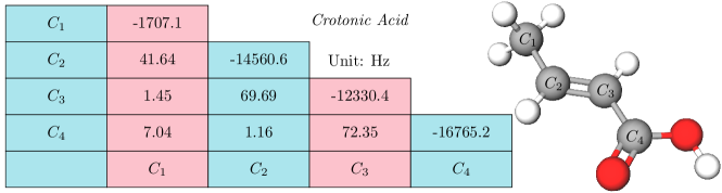
Figure 2: Structure and parameters of trans-crotonic acid. The diagonal and off-diagonal elements in the table are the chemical shifts of spins and J-coupling strengths between spins, respectively.

For NMR system, the well-established method for initialization is to prepare the qubits in the pseudo-pure state (PPS)

$$\rho_{PPS}=\frac{1-\epsilon}{16}\mathds{1}^{\otimes 4}+\epsilon\ket{0000}\bra{0000},$$ (8)

where $\mathds{1}$ is the qubit identity operator and $\epsilon\approx 10^{-5}$ is the polarization Xin_2018.

A general implementation procedure for simulating the qubit gen-extreme superchannel in Fig. 1 with our 4-qubit NMR quantum processor can be achieved as follows.

1. Preparing $\rho_{\text{in}}$. The whole system is first initialized into a PPS by using the spatial average technique cory1997ensemble, $\rho_{PPS}\simeq\ket{0000}$, starting from the thermal equilibrium state. Then an arbitrary $\rho_{\text{in}}$ can be prepared afterwards by applying a single-qubit rotation $R_{\phi}(\theta)$ to the work qubit.

2. Constructing superchannel $\hat{\mathcal{S}}$. This mainly includes applying a pre-operator $V$, an input channel $U$, and a post-operator $W$ sequentially. In general, the three multi-qubit gates can be decomposed into a sequence of single-qubit gates and two-qubit controlled gates with the cosine–sine decomposition (CSD) scheme mottonen2004quantum; Wang16. Here we packed each operator into an individual GRAPE pulse for higher fidelities in experiment, while maintaining the basic structure of superchannels.

3. Measuring $\rho_{\text{out}}$. Here $\rho_{\text{out}}$ can be reconstructed through $\rho_{\text{out}}=\mathds{1}/2+\sum_{i\in\{x,y,z\}}c_{i}\sigma_{i}$ by performing standard quantum state tomography (QST), where the Pauli components $\sigma_{x}$ and $\sigma_{y}$ of $\rho_{\text{out}}$ can be directly obtained from the spectrum of the work qubit by tracing out the rest qubits, while component $\sigma_{z}$ can be obtained in the same way by applying a $\nicefrac{{\pi}}{{2}}$ rotation readout pulse along the $X$ axis to the work qubit before the measurement.

In the following, we show how to select $\rho_{\text{in}}$ at the first stage of the above procedure, to achieve the three operators in the second stage, and to characterize the performance of the simulated superchannel with the measured $\rho_{\text{out}}$ at the last stage in experiment.

In general, to experimentally determine the dynamics of a channel $\mathcal{E}$ on an arbitrary single-qubit quantum state $\rho_{\text{in}}=\tiny{\begin{bmatrix}0.5+a&b-ic\\ b+ic&0.5-a\\ \end{bmatrix}}$ ($a$, $b$ and $c$ are all real numbers), preparation and measurement of a quantum state set $\mathcal{B}$ composed of four states are sufficient doi:10.1080/09500349708231894, such that the output state of $\rho_{\text{in}}$ under $\mathcal{E}$, $\rho_{\text{out}}$, can be constructed from the measurement result, $\mathcal{E}(\mathcal{B})$. In our scheme, we select the quantum state set as $\mathcal{B}=\{\ket{z},\ket{\bar{z}},\ket{x},\ket{y}\}$, where $\ket{z}=\ket{0}$, $\ket{\bar{z}}=\ket{1}$, $\ket{x}=(\ket{0}+\ket{1})/\sqrt{2}$ and $\ket{y}=(\ket{0}+i\ket{1})/\sqrt{2}$, which can form an arbitrary quantum state, pure or mixed, by linear combination. In this case, the output state of an arbitrary quantum state $\rho_{\text{in}}$ under the quantum channel $\mathcal{E}$ is

$$\rho_{\text{out}}=\mathcal{E}(\rho_{\text{in}}) = (0.5+a-b-c)\mathcal{E}(\ket{z}\bra{z})+(0.5-a-b-c)\mathcal{E}(\ket{\bar{z}}\bra{\bar{z}})$$ (9)

$$+2b\mathcal{E}(\ket{x}\bra{x})+2c\mathcal{E}(\ket{y}\bra{y}).$$

At the stage of constructing superchannel $\hat{\mathcal{S}}$, to achieve the optimal control, GRAPE is utilized to pack each of the three unitary operators into one shaped pulse. All shaped pulses are calculated with their fidelities reaching $99.5\%$ and are guaranteed to be robust to the inhomogeneity of radio-frequency pulses.

At the last stage, we exploit a measure of state fidelity for an arbitrary input state $\rho$ under an ideal channel $\mathcal{E}$ and its experimentally achieved channel $\mathcal{E}^{\prime}$. The unattenuated state fidelity $F_{s}$ is

$$F_{s}:=\frac{\operatorname{Tr}\left[\mathcal{E}(\rho)\mathcal{E}^{\prime}(\rho)\right]}{\sqrt{\operatorname{Tr}\left[\mathcal{E}(\rho)^{2}\right]\operatorname{Tr}\left[\mathcal{E}^{\prime}(\rho)^{2}\right]}},$$ (10)

where $\mathcal{E}(\rho)$ and $\mathcal{E}^{\prime}(\rho)$ are the ideal and experimental output density matrices corresponding to input $\rho$, and $\mathcal{E}^{\prime}(\rho)$. Thus, $\rho_{\text{out}}$ in experiment, can be obtained through QST. $F_{s}$ quantifies the similarity of $\mathcal{E}(\rho)$ and $\mathcal{E}^{\prime}(\rho)$ in ‘direction’ fortunato2002design, and is mostly used for measuring the experimental result in the NMR quantum information processing which mitigates the attenuated magnetization caused by dissipation during the unitary operation. Similar to the state fidelity definition, the process fidelity between the ideal and experimental realized channel is denoted as

$$F_{p}=\frac{\left|\operatorname{Tr}[\chi_{\text{exp}}\chi_{\text{th}}^{\dagger}]\right|}{\sqrt{\operatorname{Tr}[\chi_{\text{th}}\chi_{\text{th}}^{\dagger}]\operatorname{Tr}[\chi_{\text{exp}}\chi_{\text{exp}}^{\dagger}]}},$$ (11)

in which $\chi_{\text{th}}$ and $\chi_{\text{exp}}$ are the respective ideal and experimentally reconstructed $\chi$ matrix of an arbitrary quantum channel zhang2012experimental, which are equivalent to their Choi states.

Following the above procedure, to change from one experiment to another, next we need to select $\phi$ and $\theta$ of $R_{\phi}(\theta)$ for a specific $\rho_{\text{in}}$ in set $\mathcal{B}$, calculate GRAPE pulses of $\text{pre-}U$ operator, $U$ and post-$U$ operator for the simulated target superchannel, and finally implement the quantum circuit, obtaining the experimental results.

III.1 Simulation of extreme superchannel

We experimentally achieve a randomly chosen extreme superchannel $\hat{\mathcal{S}}$ in the NMR system, as the circuit shown in Fig. 3(a), where $C_{2}$ act as the work qubit with $C_{1}$, $C_{3}$ and $C_{4}$ serving as ancillary qubits. Starting from $\ket{0}^{\otimes 4}$, a single-qubit rotation $R_{\phi}(\theta)$ is chosen to act on $C_{2}$ to prepare $\rho_{in}$. For instance, $R_{\phi}(\theta)=R_{y}(\pi/2)$ can generate $\rho_{in}=\ket{x}$. An original random channel $\mathcal{E}$ on the work qubit $C_{2}$ is achieved through a random two-qubit unitary operator $U$ applying to $C_{1}$ and $C_{2}$, and then measuring $C_{1}$ in the final stage, where $C_{1}$ acts as the ancilla. By performing pre operator $V$ and post operator $W$ on $C_{2}$, $C_{3}$ and $C_{4}$, where $C_{3}$ and $C_{4}$ act as ancilla, and then measuring $C_{3}$ and $C_{4}$ at the same time, we successfully convert the original channel $\mathcal{E}$ into $\hat{\mathcal{S}}(\mathcal{E})$. The output state $\rho_{out}$ of the work qubit $C_{2}$ is $\hat{\mathcal{S}}(\mathcal{E})(\rho_{in})$, which can be further reconstructed with the QST. In our experiment, the length of GRAPE pulse for implementing $V$, $U$ and $W$ in experiment are 30 ms, 20 ms and 30 ms. More details of the original random channel $\mathcal{E}$, unitary operators $V$ and $W$ can be found in Appendix A.

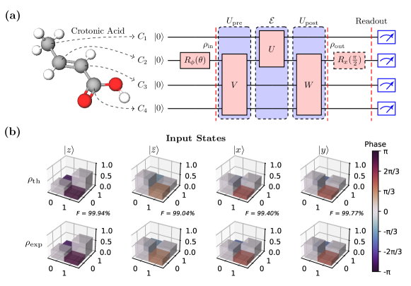
Figure 3: (a) Quantum circuit for simulating a random extreme superchannel $\hat{\mathcal{S}}(\mathcal{E})$ in experiment. $\rho_{\text{in}}$ is prepared by applying a rotation $R_{\phi}(\theta)$ to $C_{2}$, and all components of $\rho_{\text{out}}$ are obtained by direct measurement or appling a readout pulse $R_{x}(\frac{\pi}{2})$ before it. (b) Theoretical (top panel) and experimental (bottom panel) output density matrices of input states $\ket{z}$, $\ket{\bar{z}}$, $\ket{x}$ and $\ket{y}$ under $\hat{\mathcal{S}}(\mathcal{E})$. The amplitude and phase of each entry of density matrices are presented by the height and color of the $3D$ bar, respectively.

The theoretical and experimental output density matrices under the quantum channel $\hat{\mathcal{S}}(\mathcal{E})$, into which the original quantum channel $\mathcal{E}$ is converted by the randomly chosen extreme superchannel $\hat{\mathcal{S}}$, are presented in Fig. 3(b), where the top (bottom) panel are the output density matrices $\rho_{\text{out}}$ in theory (experiment) corresponding to the four input bases of $\mathcal{B}$. The fidelities $F_{s}$ between the theoretical and experimental output density matrices of $\ket{z}$, $\ket{\bar{z}}$, $\ket{x}$ and $\ket{y}$ under the converted channel $\hat{\mathcal{S}}(\mathcal{E})$ are $99.94\%$, $99.04\%$, $99.40\%$ and $99.77\%$, respectively, indicating a very good simulation of the converted channel $\hat{\mathcal{S}}(\mathcal{E})$ in our experiment. For comparison, we also reconstruct the original channel $\mathcal{E}$, the theoretical and experimental output density matrices under which can be found in Appendix A.

To generalize our simulation result of the randomly chosen superchannel $\hat{\mathcal{S}}$, 1000 input states are sampled on the Bloch sphere surface (green dots in Fig. 4(a)) based on the spherical Fibonacci lattice method, of which the output states can be reconstructed by the measured output states of the four states (9). For comparison, the theoretical and experimental output states of the original random channel $\mathcal{E}$ are presented as the blue dots in Fig. 4(a), while that of $\hat{\mathcal{S}}(\mathcal{E})$ are plotted as the red dots. The experimental results of $\mathcal{E}$ and $\hat{\mathcal{S}}(\mathcal{E})$ are in good agreement with their theoretical ones, and the significant difference between the output results of $\mathcal{E}$ and $\hat{\mathcal{S}}(\mathcal{E})$ indicates the success of converting the original channel $\mathcal{E}$ into $\hat{\mathcal{S}}(\mathcal{E})$ by superchannel $\hat{\mathcal{S}}$.

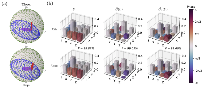
Figure 4: (a) Input and output states sampled in the Bloch sphere. Theoretical (top panel) and experimental (bottom panel) output states corresponding to the input states (green dots) after a random channel (blue dots), a gen-extreme superchannel (red dots) and a dephasing superchannel (purple dots). (b) Theoretical (top panel) and experimental (bottom panel) $\chi$ matrices of the random channel $\mathcal{E}$, converted channels $\hat{\mathcal{S}}(\mathcal{E})$ and $\hat{\mathcal{S}}_{d}(\mathcal{E})$.

To fully characterize the original channel $\mathcal{E}$ and the converted channel $\hat{\mathcal{S}}(\mathcal{E})$, quantum process tomography (QPT) NC00 was conducted, and $\chi_{\text{exp}}$ matrices of both channels were reconstructed from the experimental QST results of our selected input state set $\mathcal{B}$. Thereafter they were transformed into the standard basis set {I, X, Y, Z}, as shown in Fig. 4(b), which reveals further evidence of successfully converting the original channel $\mathcal{E}$ into $\hat{\mathcal{S}}(\mathcal{E})$ by superchannel $\hat{\mathcal{S}}$ – dramatic difference in the amplitude and phase of entries of $\mathcal{E}$ and $\hat{\mathcal{S}}(\mathcal{E})$. The process fidelities of the ideal channel $\mathcal{E}$ and the experimentally achieved channel $\hat{\mathcal{S}}(\mathcal{E})$ are $99.82\%$ and $99.02\%$, respectively, which implies a good verification of accurate channel simulation of $\mathcal{E}$ and $\hat{\mathcal{S}}(\mathcal{E})$, and further proving the accurate simulation of superchannel $\hat{\mathcal{S}}$.

III.2 Simulation of dephasing superchannel

The dephasing superchannel is also gen-extreme PKS+21. In a fixed basis, it is defined to preserve the diagonal elements of the input Choi states while suffering a phase noise which alters the non-diagonal elements. Actually, if we consider dephasing channels acting on $d^{2}$-dimensional systems, then it is easy to obtain that a dephasing superchannel is of the form of dephasing channels.

The experimental circuit is shown in Fig. 5(a). With similar method with the previous experiment, here we use controlled-$V_{i}$ and controlled-$W_{i}$ (targetting at $C_{3}$ and $C_{4}$ with $C_{2}$ as the control qubit, and $i\in\{1,2\}$) as the pre and post operators to construct a dephasing superchannel. as the input channel only acts on the control unit, the diagonal elements of the input Choi states stays the same. More details of unitary operators $V_{i}$ and $W_{i}$ ($i\in\{1,2\}$) can be found in Appendix A.

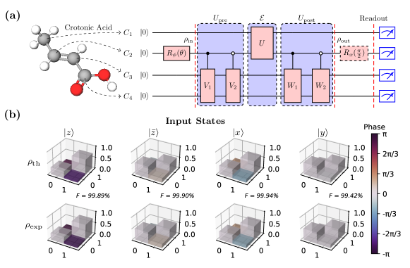
Figure 5: (a) Quantum circuit for simulating a random extreme superchannel $\hat{\mathcal{S}}_{d}(\mathcal{E})$ in experiment. (b) Theoretical (top panel) and experimental (bottom panel) output density matrices of input states $\ket{z}$, $\ket{\bar{z}}$, $\ket{x}$ and $\ket{y}$ under $\hat{\mathcal{S}}_{d}(\mathcal{E})$.

The whole experiment proceeds as before, the random channel $\mathcal{E}$ is preserved, i.e., keeping $U$ unchanged, while the controlled-$V_{i}$s and controlled-$W_{i}$s are packed into two individual GRAPE pulses with length of 22 ms and 25 ms, respectively. The same state set $\mathcal{B}$ is selected as the input of our simulated channel, and the output density matrices are presented in Fig. 5(b). The state fidelities $F_{s}$ between the theoretical and experimentally reconstructed density matrices corresponding to the four input states under the channel $\hat{S}_{d}(\mathcal{E})$ are $99.89\%$, $99.90\%$, $99.94\%$ and $99.42\%$, respectively. Besides, to characterize the function of $\hat{\mathcal{S}}_{d}$, one way is to compare the output state of an arbitrary input state before and after the application of dephasing superchannel $\hat{\mathcal{S}}_{d}$.

The sampled theoretical and experimental output states of the converted channel $\hat{\mathcal{S}}_{d}(\mathcal{E})$ are presented as the purple dots in Fig. 4(a), which shows the experimental results of $\hat{\mathcal{S}}_{d}(\mathcal{E})$ are in good agreement with their theoretical ones, and successfully converting the original channel $\mathcal{E}$ (blue dots) into another channel $\hat{\mathcal{S}}_{d}(\mathcal{E})$ by a random dephasing superchannel $\hat{\mathcal{S}}_{d}$. An alternative way is to reconstruct the process matrices $\chi$ before and after applying $\hat{\mathcal{S}}_{d}$, as shown in Fig. 4(b). The process fidelity $F_{p}$ between the ideal and experimentally reconstructed $\chi$ matrices of the converted channel $\hat{\mathcal{S}}_{d}(\mathcal{E})$ achieves $99.60\%$. In a nutshell, both facts indicate a very good simulation of the dephasing superchannel $\hat{\mathcal{S}}_{d}$ in our experiment.

For comparison, the ideal and experimental Choi states of channels $\mathcal{E}$, $\hat{\mathcal{S}}(\mathcal{E})$ and $\hat{\mathcal{S}}_{d}(\mathcal{E})$ are reconstructed based on the $\chi$ matrices, and presented in Fig. 6. It shows the dephasing superchannel $\hat{\mathcal{S}}_{d}$ causes the dephasing of Choi state $\omega_{\mathcal{E}}$ of the random channel $\mathcal{E}$ — compressing the amplitude of non-diagonal elements while leaving the diagonal elements unchanged. However, a random superchannel $\hat{\mathcal{S}}$ (see subfigures in the middle of Fig. 6) does not have that feature in general.

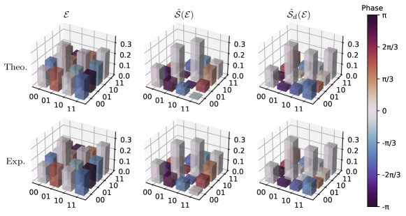
Figure 6: Choi state matrices of channel $\mathcal{E}$, $\hat{S}(\mathcal{E})$ and $\hat{S}_{d}(\mathcal{E})$. The top (bottom) panel shows the respective Choi state matrix reconstructed from the theoretical (experimental) Choi state matrices of the random channel $\mathcal{E}$, $\hat{S}(\mathcal{E})$ and $\hat{S}_{d}(\mathcal{E})$.

III.3 Demonstration of superchannel decomposition

We experimentally demonstrate the decomposition of a general superchannel $\hat{\mathcal{S}_{g}}$. Restricted by our experimental apparatus, we choose the input channel as an unitary operator $U$ and design our quantum circuit by constructing a random non-extreme superchannel with randomly chosen $V$ and $W$, as shown in the left panel of Fig. 7(a). We demonstrate that this 4-qubit-composed superchannel can be decomposed into two 3-qubit-composed extreme superchannels. Here, we choose $V_{i}$ and $W_{i}$ using composition with equal $p_{i}$ (6). Therefore, for an arbitrary input channel $U$ and an arbitrary input state $\rho_{\text{in}}$, the output state under the general superchannel $\hat{\mathcal{S}_{g}}$, which is $\rho_{\text{out}}$ can be approximated as the average of the output states $\rho_{\text{out}}^{1}$ and $\rho_{\text{out}}^{2}$ under the two extreme superchannels $\hat{\mathcal{S}_{g}^{1}}$ and $\hat{\mathcal{S}_{g}^{2}}$, i.e., $\rho_{\text{out}}\approx(\rho_{\text{out}}^{1}+\rho_{\text{out}}^{2})/2$.

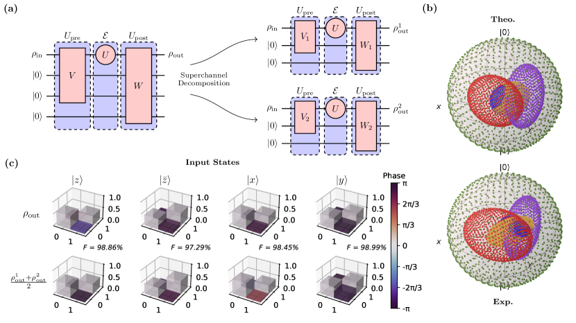
Figure 7: (a) Superchannel convex-decomposition scheme. A random superchannel simulated in 4 qubits can be decomposed into two 3-qubit extreme superchannles. (b) Theoretical (top panel) and experimental (bottom panel) output states in the Bloch sphere. The green, blue, red, purple and orange dots represent the sampled input states $\rho_{\text{in}}$, corresponding output states $\rho_{\text{out}}$, $\rho_{\text{out}}^{1}$, $\rho_{\text{out}}^{2}$, and $(\rho_{\text{out}}^{1}+\rho_{\text{out}}^{2})/2$, respectively. (c) Experimental output density matrices in our superchannel convex-decomposition scheme. (Top panel) The output states $\rho_{\text{out}}$ of $\hat{\mathcal{S}_{g}}$ in $\ket{z}$, $\ket{\bar{z}}$, $\ket{x}$ and $\ket{y}$ basis, while the bottom panel shows the average of the output states under its decomposed two superchannels, $(\rho_{\text{out}}^{1}+\rho_{\text{out}}^{2})/2$.

In our scheme, three groups of experiments corresponding to the circuits in Fig. 7(a) were conducted, where $U$, $V$ and $W$ are generated randomly, while two pairs of $V_{i}$ and $W_{i}$ ($i\in\{1,2\}$) are calculated based on $V$ and $W$. See Appendix A for more details of unitary operators $U$, $V$, $W$, $V_{i}$ and $W_{i}$ ($i\in\{1,2\}$). We pack each unitary operator $V$, $U$, $W$ of the three circuits into an individual GRAPE pulse. The input states $\rho_{in}$ are selected from the input state set $\mathcal{B}$, after which the QST process on $C_{1}$ is performed to reconstruct the output state $\rho_{out}$, $\rho_{out}^{1}$ and $\rho_{out}^{2}$. The theoretical and experimental output states are illustrated in Appendix A. The state fidelities $F_{s}$ obtained range from $97.28\%$ to $99.96\%$, where the lower fidelities mainly come from the 4-qubit-composed superchannel circuit whose unitary operators $V$ and $W$ are more complicated, thus the total pulse length of the circuit from preparing pseudo-pure state to making measurements reaches 165 ms, causing larger decoherence effect of $T_{2}$.

As before, the theoretical and experimental output states of $1000$ input states, which are sampled based on the spherical Fibonacci lattice, under the original superchannel $\hat{\mathcal{S}_{g}}$ and the two extreme superchannels $\hat{\mathcal{S}_{g}^{1}}$ and $\hat{\mathcal{S}_{g}^{2}}$ presented in Fig. 7(b), separately. The output states of the sampled input states under the general superchannel $\hat{\mathcal{S}_{g}}$ are illustrated in blue dots, while that under extreme superchannels $\hat{\mathcal{S}_{g}^{1}}$ and $\hat{\mathcal{S}_{g}^{2}}$ are illustrated in red and purple dots. The theoretical and experimental output states are in good agreement (the comparatively bad agreement of blue dots corresponding to simulating $\hat{\mathcal{S}_{g}}$ can be attributed to the decoherence effect of $T_{2}$), indicating a well simulation of each superchannel in experiment.

To demonstrate the implementation of the convex-decomposition of a random superchannel $\hat{\mathcal{S}_{g}}$ in experiment, we reconstruct the averaged states of the experimental outputs of our selected inputs under the two extreme superchannels $\hat{\mathcal{S}_{g}^{1}}$ and $\hat{\mathcal{S}_{g}^{2}}$, and compare them with their corresponding experimental output states under the original superchannel $\hat{\mathcal{S}_{g}}$, as shown in Fig. 7(c). Besides, we calculated the fidelities between the corresponding states in the top panel and the bottom panel of Fig. 7(c), which are $98.86\%$, $97.29\%$, $98.45\%$ and $98.99\%$, respectively. Furthermore, the theoretical and experimental averaged output states of $1000$ sampled input states corresponding to the two extreme superchannels $\hat{\mathcal{S}_{g}^{1}}$ and $\hat{\mathcal{S}_{g}^{2}}$ are presented in orange dots in Fig. 7(b), as a comparison with the original output states (blue dots). The mismatch of them in experiment (blue and orange dots in the bottom panel of Fig. 7(b)) is mainly concentrated on the data in the Bloch sphere along the positive $x$-axis and negative $z$-axis, which are dominated by our imperfect experimental realization of the original superchannel $\hat{\mathcal{S}_{g}}$.

IV Summary

In this paper, we experimentally realized an algorithm-assisted NMR simulator of qubit superchannels. We demonstrate our simulator with three simulation tasks, including a random extreme superchannel, a dephasing superchannel and a superchannel convex-decomposition scheme. Furthermore, our experimental result also shows that the superchannel achieved by convex-decomposition has a higher fidelity than that achieved directly, on account of the less number of qubits involved in the circuit realization. The experimentally simulated superchannels are in great agreement with their theoretical counterparts. Our experiment verifies the feasibility of the convex channel-decomposition algorithm, implying the promising usage of it for higher-dimensional cases and other tasks.

Appendix A Details of experiments

A.1 Random channel

In our scheme, a random channel $\mathcal{E}$ is implemented by a two-qubit unitary with one qubit as the work qubit and the other as an ancilla, and a random chosen $U$ can be found (12). A circuit for simulating a random channel with our $4$-qubit NMR quantum processor can be found in Fig. 8(a), where $C_{2}$ serves as the work qubit and $C_{1}$ as the ancilla. The entire system is initialized in the pseudo-pure state $\ket{0000}$ from the thermal equilibrium state with the spatial average technique at first, and $U$ can be decomposed into a sequence of single-qubit gates and two-qubit controlled gates with the cosine–sine decomposition (CSD) scheme mottonen2004quantum.

$$U=\begin{bmatrix}-0.0109+0.1787i&-0.2558-0.1492i&-0.2519+0.2656i&-0.4561-0.7336i\\ -0.6709-0.2262i&0.1270-0.1671i&0.4623-0.3549i&-0.3017-0.1551i\\ -0.1406-0.5049i&-0.2872-0.5841i&-0.4014+0.1515i&-0.0718+0.3353i\\ 0.3717-0.2321i&-0.6624+0.0766i&0.1922-0.5526i&0.0420-0.1389i\end{bmatrix}.$$ (12)

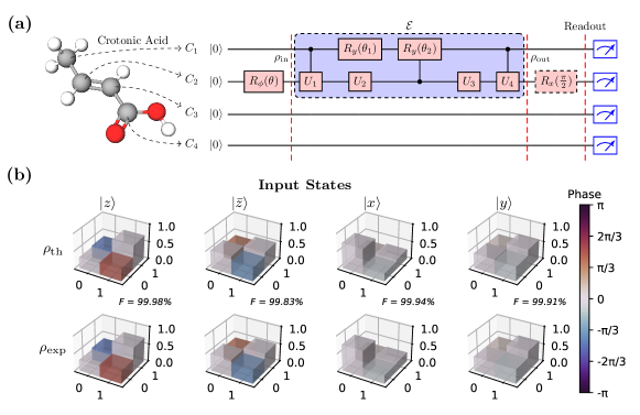
Figure 8: (a) Quantum circuit for simulating a random extreme superchannel $\mathcal{E}$ in experiment. (b) Theoretical (top panel) and experimental (bottom panel) output density matrices of input states $\ket{z}$, $\ket{\bar{z}}$, $\ket{x}$ and $\ket{y}$ under $\mathcal{E}$.

The output density matrices of the input state bases under the random channel $\mathcal{E}$ in theory and experiment are presented in Fig. 8(b). The state fidelities between the theoretical and experimental density matrices of $\ket{z}$, $\ket{\bar{z}}$, $\ket{x}$ and $\ket{y}$ under the channel $\mathcal{E}$ are $99.98\%$, $99.83\%$, $99.94\%$ and $99.91\%$, respectively.

A.2 Extreme superchannel

To simulate a random extreme superchannel, two random unitary pre-$U$ (V) and post-$U$ (W) operations of the superchannel $\hat{\mathcal{S}}$ are generated as follows,

$$V={\tiny\begin{bmatrix}0.1310+0.0036i&0.1140-0.2525i&-0.0068+0.1055i&-0.0556-0.1594i&-0.1454-0.1854i&0.0073-0.3811i&0.2214-0.0904i&0.3471-0.6985i\\ -0.1604-0.2878i&-0.1567-0.0025i&0.0613-0.1076i&-0.2527+0.1187i&-0.0739-0.7163i&0.1182-0.0921i&0.2490-0.3120i&-0.0706+0.2611i\\ 0.0732+0.3537i&-0.4630+0.0267i&0.0920+0.0445i&0.2267+0.2262i&0.1608-0.0286i&0.5365+0.2132i&-0.0708-0.3283i&-0.0228-0.2614i\\ -0.0093+0.1815i&0.1717+0.0019i&0.6431-0.1916i&-0.2676-0.0393i&0.2835-0.0428i&-0.2191-0.0210i&-0.4000-0.2678i&0.2271+0.0038i\\ 0.0826-0.2314i&-0.4620-0.2645i&0.5516+0.0022i&0.2165-0.1446i&-0.3134+0.0563i&0.0363-0.0046i&0.0473+0.3653i&0.1578+0.1447i\\ -0.1508-0.4899i&0.3662-0.0245i&0.1410+0.0025i&-0.2153-0.0342i&-0.1672+0.2146i&0.5844+0.2191i&-0.1869-0.0348i&-0.0823-0.1694i\\ 0.2754+0.0592i&-0.3809-0.1076i&-0.3006+0.1213i&-0.6761-0.1579i&-0.0537+0.1575i&0.1289-0.1106i&-0.2538+0.0173i&0.1640+0.1696i\\ -0.2048+0.5161i&0.0955+0.2651i&0.2211+0.1859i&-0.3256-0.1205i&-0.2508-0.2259i&0.1189+0.1293i&0.1400+0.4275i&-0.2195-0.1139i\end{bmatrix}},$$ (13)

$$W={\tiny\begin{bmatrix}0.4438+0.3052i&-0.1516-0.1924i&0.1702-0.2479i&0.1763+0.1283i&0.0741+0.1495i&-0.0073-0.2209i&-0.5178+0.0332i&-0.4073-0.0107i\\ 0.2915+0.1024i&0.1375-0.0168i&-0.3881-0.2651i&0.0306+0.0003i&-0.1106+0.3559i&0.2050+0.3621i&-0.1741+0.0693i&0.5075-0.2425i\\ -0.0480-0.2797i&0.0909-0.0858i&0.1075-0.1673i&-0.3236-0.0472i&0.1355+0.3724i&-0.3431-0.5753i&-0.1038-0.1457i&0.3381-0.0721i\\ -0.3029+0.1556i&0.1901+0.4494i&-0.0179-0.1726i&0.0388-0.2170i&0.0461-0.3691i&0.1803-0.2864i&-0.4075+0.3044i&0.1226-0.2016i\\ 0.1913+0.3040i&-0.1178+0.5217i&0.2078-0.0749i&-0.2228-0.3476i&0.3159+0.2880i&-0.0994+0.1536i&0.3143-0.0292i&-0.1557-0.1599i\\ 0.3786+0.0292i&-0.1600+0.0010i&0.3856+0.4572i&-0.3605+0.1393i&-0.0270-0.2707i&-0.0489+0.1073i&-0.1928+0.2379i&0.3690-0.0730i\\ -0.0113+0.0191i&0.5498+0.1459i&0.2502+0.3443i&0.4872+0.1597i&0.2423+0.3037i&-0.1340+0.0581i&-0.0583+0.1419i&0.0926+0.1658i\\ -0.0737+0.3725i&-0.1613-0.0762i&-0.0488-0.1704i&-0.0245+0.4611i&0.3602-0.0189i&0.2744-0.2661i&0.3682+0.2291i&0.2555+0.2231i\end{bmatrix}}.$$ (14)

A.3 Dephasing superchannel

To simulate a random dephasing superchannel, random unitary pre-$U$ and post-$U$ operations of the superchannel $\hat{\mathcal{S}}_{d}$, controlled-$V_{i}$ and controlled-$W_{i}$ ($i\in\{1,2\}$), are generated. The generated $V_{i}$ and $W_{i}$ are as follows,

$$V_{1}=\begin{bmatrix}0.2987+0.2302i&0.4874-0.2877i&0.1190+0.2665i&-0.6694+0.0645i\\ 0.0898+0.2401i&-0.5247-0.5788i&-0.3600+0.2082i&-0.0291-0.3876i\\ 0.7734-0.1597i&0.1368+0.1863i&-0.5275-0.1207i&0.1707+0.0293i\\ -0.4084+0.0403i&-0.0644+0.1087i&-0.6699+0.0164i&-0.3253+0.5107i\end{bmatrix},$$ (15)

$$V_{2}=\begin{bmatrix}-0.5089+0.0961i&-0.3067+0.4412i&0.0754+0.5513i&-0.2788-0.2359i\\ -0.1870-0.2108i&0.2685+0.6255i&-0.5304-0.2773i&0.0053+0.3145i\\ 0.5061+0.0705i&-0.0278-0.1007i&-0.4042+0.3316i&-0.6458+0.1939i\\ 0.5896-0.2091i&0.1698+0.4562i&0.0943+0.2234i&0.2692-0.4904i\end{bmatrix},$$ (16)

$$W_{1}=\begin{bmatrix}-0.2919+0.0605i&-0.6294-0.6274i&0.1046-0.0290i&0.3088+0.1191i\\ 0.2956-0.0233i&-0.0973-0.4107i&-0.3067-0.1554i&-0.3989-0.6758i\\ -0.3639+0.7948i&0.1587-0.0780i&-0.2993+0.2414i&-0.2318+0.0552i\\ -0.0806-0.2295i&0.0100+0.0259i&-0.1371+0.8387i&0.3037-0.3545i\end{bmatrix},$$ (17)

$$W_{2}=\begin{bmatrix}-0.6174+0.3184i&0.4179-0.3318i&0.2918+0.0792i&0.3384+0.1635i\\ -0.5162-0.4553i&-0.5212-0.1814i&0.2151-0.1841i&-0.0083-0.3761i\\ -0.1403+0.0197i&-0.4111-0.4270i&-0.5477+0.1773i&-0.0179+0.5448i\\ 0.1005+0.1163i&-0.1773-0.1668i&0.6157+0.3434i&-0.6002+0.2446i\end{bmatrix}.$$ (18)

A.4 Superchannel convex-decomposition

To simulate a general superchannel $\hat{\mathcal{S}}_{g}$ and its decomposed superchannels $\hat{\mathcal{S}}_{g}^{1}$ and $\hat{\mathcal{S}}_{g}^{2}$ in Fig. 7(a), the input unitary channel $U$, pre-$U$ operator V, and post-$W$ are generated randomly as follows. Then two pairs of pre-$U$ operator $V_{i}$ and post-$U$ operator $W_{i}$ corresponding to each decomposed superchannel are calculated ($i\in\{1,2\}$).

$$U={\footnotesize\begin{bmatrix}0.6196+0.2891i&0.5199-0.5120i\\ -0.7191+0.1236i&0.1266-0.6720i\end{bmatrix}},$$ (19)

$$V={\tiny\begin{bmatrix}-0.3048+0.1792i&-0.1955+0.1514i&-0.1071+0.4419i&-0.2905+0.4894i&0.0582-0.0069i&0.3937+0.0449i&0.1629-0.0733i&0.2968+0.0526i\\ -0.2444+0.2554i&0.3402-0.3981i&-0.38-0.0044i&-0.0067+0.1559i&-0.3934-0.1094i&-0.2565-0.1723i&-0.2516+0.1297i&0.2637-0.1417i\\ -0.0471-0.3504i&0.1682-0.1016i&-0.4623-0.0185i&0.3695+0.2124i&0.4099+0.1691i&0.1721+0.1661i&-0.086-0.2099i&-0.0726-0.3607i\\ -0.3144+0.1616i&-0.2029+0.0234i&-0.2241-0.1805i&0.2492-0.0861i&-0.3302+0.2253i&-0.0083-0.1936i&0.3955-0.4893i&-0.2484+0.1617i\\ 0.1437+0.323i&0.1932+0.2012i&-0.1963+0.0867i&-0.2034+0.0288i&0.1726-0.4514i&-0.3652+0.2439i&0.3478-0.1881i&-0.2604-0.2417i\\ 0.3028+0.1824i&0.0162+0.1912i&-0.36-0.0257i&0.4639-0.1851i&-0.053-0.21i&0.2402+0.1343i&0.2099+0.2835i&0.3502+0.2979i\\ -0.3514+0.0389i&-0.0504-0.2043i&0.375-0.0656i&0.225-0.191i&0.0744-0.1392i&-0.1365+0.5133i&0.0526-0.2765i&0.4555-0.07i\\ -0.0019+0.3535i&0.5216-0.3915i&0.1607-0.0696i&-0.112-0.0962i&0.3056+0.2732i&0.3194-0.0075i&0.279+0.0544i&-0.1099+0.1849i\\ \end{bmatrix}},$$ (20)

$$\begin{split}W={\tiny\left[\begin{matrix}0.2496+0.0149i&0.2583+0.094i&-0.142-0.1203i&0.0349-0.3243i&-0.0593-0.2491i&0.1259-0.1864i&0.2037-0.0822i&-0.0785+0.048i\\ -0.2373+0.0788i&-0.3037+0.126i&-0.0402+0.1706i&-0.0718+0.23i&-0.1582+0.1418i&0.1646-0.1858i&0.1247-0.1802i&-0.2847+0.1219i\\ -0.2248+0.1095i&0.1179-0.1226i&0.1822+0.0558i&-0.0741+0.2566i&-0.1138-0.1522i&-0.0315-0.2075i&0.2547-0.1522i&0.0425-0.2004i\\ -0.1901+0.1623i&0.3132+0.0882i&0.0661-0.1666i&-0.284+0.0335i&0.0413+0.2787i&-0.1569+0.0769i&-0.1572+0.1256i&-0.0615+0.1315i\\ -0.0658-0.2412i&-0.0596+0.248i&0.0867-0.3673i&-0.237+0.2021i&-0.0141+0.0435i&-0.0651+0.3i&0.0707-0.0175i&0.4078-0.1094i\\ 0.1712-0.1822i&0.1187+0.1043i&0.3132+0.1139i&-0.1399+0.1597i&0.2434+0.0886i&0.3244-0.0918i&0.0191+0.1291i&-0.1523-0.1812i\\ -0.2493-0.0189i&0.2004+0.2046i&-0.0233+0.191i&0.2898-0.1628i&-0.1203-0.0997i&0.1576+0.2563i&-0.1431+0.1529i&0.0233-0.1447i\\ -0.2374-0.0784i&0.1884+0.0826i&0.1236+0.1263i&0.2088+0.0682i&0.0835-0.1652i&-0.1811-0.1144i&0.2168-0.2539i&0.2162+0.1115i\\ -0.1046-0.2271i&0.0901-0.1779i&-0.2164-0.0362i&0.0399-0.2029i&0.1211-0.0554i&-0.3369-0.084i&-0.0279+0.3642i&-0.116+0.0211i\\ -0.1484-0.2012i&0.1407-0.0525i&-0.2549-0.0569i&0.2266-0.0998i&-0.1081+0.474i&0.0232+0.0294i&0.2458-0.2511i&0.0353+0.0316i\\ -0.2351+0.0851i&0.1065-0.1222i&-0.0901+0.2486i&-0.0477+0.2347i&0.2255-0.0802i&-0.0224-0.174i&-0.1716+0.1242i&0.237+0.0908i\\ -0.2241-0.1109i&-0.266-0.1549i&-0.0406+0.1548i&0.2583-0.0425i&-0.179+0.1142i&-0.0059-0.0271i&-0.0212+0.3362i&0.0442+0.0525i\\ 0.0403-0.2467i&0.1307+0.0725i&0.1723+0.2049i&0.2006-0.0199i&0.1575-0.1724i&0.038+0.4326i&0.0355-0.1262i&-0.2927+0.3575i\\ -0.0077-0.2499i&-0.2569+0.1936i&-0.0661+0.122i&-0.0947-0.1935i&0.1183-0.2758i&-0.0135-0.1952i&-0.1709-0.2207i&0.0604-0.3126i\\ 0.2175+0.1234i&-0.053+0.1559i&-0.23+0.2018i&0.0436+0.1896i&-0.3336-0.0763i&0.1976-0.1153i&-0.1811+0.0747i&0.1895+0.2625i\\ 0.2498-0.0112i&0.3396-0.1248i&-0.0057+0.3846i&-0.1327+0.0958i&-0.164-0.0312i&-0.0961+0.1644i&0.0943-0.1998i&0.0498-0.1012i\\ \end{matrix}\right.}\\ {\tiny\left.\begin{matrix}-0.0784-0.2447i&-0.1059-0.187i&0.2683+0.1565i&0.027-0.3735i&0.0801-0.182i&0.0589+0.1512i&0.1614-0.0585i&-0.1959+0.2558i\\ 0.1948+0.2293i&0.048-0.3343i&0.0701-0.1766i&-0.0728-0.1856i&-0.0705-0.2182i&-0.2751+0.0986i&0.2089+0.1523i&0.0045+0.0682i\\ 0.0825-0.1661i&-0.2516+0.2799i&-0.1183+0.2518i&-0.2201+0.0661i&0.1242-0.2592i&-0.22+0.0525i&-0.2873-0.0038i&-0.2517-0.0691i\\ -0.157-0.0736i&0.022+0.1112i&-0.235-0.3061i&0.1081-0.2763i&0.1078+0.0399i&-0.1089-0.0951i&-0.0276+0.2065i&-0.333+0.2794i\\ -0.0824-0.1228i&-0.0549-0.1076i&0.2991+0.014i&-0.0186+0.1768i&-0.0352-0.052i&-0.3052+0.1329i&0.266-0.0877i&-0.0168+0.0436i\\ 0.1974+0.17i&-0.148+0.161i&0.1659+0.0188i&-0.0182+0.2201i&-0.105-0.0469i&0.2984-0.1923i&0.1901+0.1128i&-0.1552+0.3129i\\ 0.1318-0.3185i&0.1564+0.0239i&0.0877-0.1062i&-0.4498-0.0141i&-0.0473-0.0824i&-0.0954-0.1962i&0.0109+0.2583i&0.1798+0.0812i\\ -0.2362+0.2337i&0.2573-0.0928i&0.0188-0.1261i&-0.1145+0.1495i&0.3622+0.0737i&0.3076+0.0484i&0.2261+0.1468i&-0.1411-0.0428i\\ 0.323+0.1483i&-0.1323-0.1395i&0.0935-0.0912i&-0.029+0.3175i&0.1167-0.0644i&-0.1258+0.3647i&-0.1169+0.1682i&-0.0955+0.1469i\\ 0.0226+0.0146i&-0.2957-0.083i&-0.0928+0.3398i&0.0924+0.0761i&-0.0457+0.2595i&-0.0453-0.2416i&0.0365+0.2071i&0.0346+0.1146i\\ -0.1721-0.1751i&0.0594-0.4234i&0.1996+0.1861i&0.205+0.0541i&-0.3586-0.0757i&0.0632-0.169i&-0.2057+0.036i&-0.1029+0.0554i\\ -0.1026-0.0207i&0.0667+0.1958i&-0.0253+0.092i&-0.0918-0.067i&-0.0848+0.0525i&-0.0045-0.0126i&0.3188-0.4419i&-0.4276+0.1375i\\ -0.2824+0.1499i&-0.1682+0.024i&-0.059-0.0036i&0.1132+0.0792i&-0.1176-0.2134i&-0.2738+0.0064i&-0.1411-0.127i&-0.0674+0.0204i\\ -0.1578-0.0919i&0.0187-0.0196i&-0.5032+0.017i&0.0682+0.0755i&-0.1524+0.0931i&-0.1336+0.0936i&0.0804+0.1285i&-0.0352+0.2828i\\ -0.0483-0.0613i&-0.1126+0.1125i&0.0355-0.063i&0.2123+0.3211i&0.4206-0.0092i&-0.1389-0.0905i&-0.0502+0.016i&0.0641+0.2646i\\ 0.3464-0.0108i&0.3327-0.0229i&0.0219-0.0296i&0.0952-0.0145i&-0.1348+0.3624i&-0.2264+0.1113i&0.0436-0.1429i&-0.1608+0.0548i\\ \end{matrix}\right]},\end{split}$$ (21)

$$V_{1}={\tiny\begin{bmatrix}-0.4371-0.2427i&-0.2991+0.0099i&-0.543-0.2371i&-0.5449+0.1117i\\ -0.4979+0.0455i&-0.0157+0.2448i&0.4424-0.5705i&0.2641+0.3145i\\ -0.3409-0.3658i&-0.2866-0.3124i&-0.213+0.2186i&0.6782-0.1312i\\ -0.4157-0.2778i&0.8157+0.0725i&-0.024+0.1845i&-0.0852-0.1938i\\ \end{bmatrix}},$$ (22)

$$W_{1}={\tiny\begin{bmatrix}0.1311+0.3283i&0.1787+0.1497i&0.2948-0.0795i&-0.1267+0.144i&-0.2625+0.1616i&0.435+0.4329i&0.348+0.2178i&-0.118+0.1909i\\ -0.3088-0.1721i&-0.0507-0.2383i&0.4115-0.0159i&0.3146-0.33i&-0.3464+0.4922i&0.0009+0.0816i&-0.1953-0.1556i&0.0655+0.0522i\\ 0.2655-0.2335i&-0.4459-0.1607i&-0.0586+0.491i&0.0964+0.1417i&0.2059+0.2077i&0.3649+0.1429i&-0.1906+0.315i&0.0052-0.0422i\\ 0.3518+0.0347i&0.2181-0.0184i&0.2035+0.2981i&-0.2619-0.1756i&0.0745+0.2214i&-0.3757-0.2796i&-0.0407+0.1763i&-0.0282+0.5385i\\ 0.1854-0.3011i&0.1739+0.4225i&0.0297+0.1532i&-0.1691-0.2287i&0.258+0.129i&0.0451+0.3754i&-0.073-0.529i&-0.1907-0.1153i\\ -0.1763-0.3065i&-0.2514-0.0616i&-0.2356+0.0748i&-0.6395-0.2149i&-0.4043-0.0311i&0.1943-0.1172i&0.2272-0.0731i&0.1031+0.091i\\ 0.2343+0.2647i&-0.5026-0.1922i&0.4268-0.0851i&-0.1434+0.0711i&-0.0345-0.3266i&0.0132-0.041i&-0.1625-0.4256i&-0.2028+0.1095i\\ 0.2445+0.2554i&0.1842+0.1208i&0.2086+0.2099i&-0.1123-0.2286i&-0.1692-0.1362i&0.1655-0.1419i&-0.2248+0.0226i&0.5754-0.444i\\ \end{bmatrix}},$$ (23)

$$V_{2}={\tiny\begin{bmatrix}-0.4008+0.299i&-0.2726-0.0633i&-0.5762+0.0519i&-0.3259-0.4804i\\ 0.3645+0.3422i&-0.2194+0.2229i&0.476-0.3105i&-0.0414-0.5723i\\ 0.0648-0.4958i&0.3064+0.0338i&0.1171+0.564i&-0.0865-0.5618i\\ -0.4988-0.034i&0.1224+0.8449i&0.0872-0.0542i&0.0955+0.039i\\ \end{bmatrix}},$$ (24)

$$W_{2}={\tiny\begin{bmatrix}-0.2271+0.271i&-0.1472+0.254i&0.321+0.1788i&0.1722-0.0949i&-0.162-0.4895i&-0.1554+0.4099i&0.1569-0.0484i&-0.3607-0.0085i\\ -0.3475+0.0651i&0.3698+0.069i&0.1526-0.0904i&-0.2671+0.0309i&-0.209-0.117i&0.1731-0.4028i&0.1465-0.143i&-0.0624-0.5782i\\ -0.1736-0.308i&-0.1436+0.287i&0.2615-0.184i&-0.2339+0.5177i&-0.0259+0.0096i&0.1182-0.0133i&-0.3389+0.3749i&-0.2362+0.1446i\\ 0.3238+0.1419i&0.142+0.3402i&-0.2921-0.2162i&-0.0305-0.208i&0.2057-0.5327i&-0.0957-0.319i&-0.3229+0.1092i&-0.0894+0.0403i\\ 0.3455+0.0751i&-0.0961+0.4293i&-0.107+0.2211i&-0.1628+0.5174i&0.0118+0.015i&-0.0694-0.1127i&0.3936-0.3791i&0.0777+0.0661i\\ 0.2639-0.2353i&-0.3539+0.0755i&0.2208-0.5372i&0.1758-0.1027i&-0.2688+0.035i&-0.38-0.0746i&0.1909+0.0368i&0.1329-0.2938i\\ -0.3046-0.1795i&-0.1508+0.2398i&0.1115+0.2248i&0.0133-0.3706i&-0.1492+0.1805i&-0.2096-0.5272i&-0.0013-0.159i&-0.0742+0.4322i\\ -0.1061+0.3373i&-0.2949+0.2044i&-0.2965+0.2251i&0.1974+0.0994i&-0.4443+0.1544i&0.0274-0.0227i&-0.4356+0.0898i&0.2576-0.2688i\\ \end{bmatrix}}.$$ (25)

The output density matrices of the input state bases in the general superchannel $\hat{\mathcal{S}}_{g}$ scheme in theory and experiment are presented in Fig. 9. The state fidelities between the theoretical and experimental density matrices of $\ket{z}$, $\ket{\bar{z}}$, $\ket{x}$ and $\ket{y}$ under the channel $\mathcal{E}$ are $98.12\%$, $97.95\%$, $97.28\%$ and $98.76\%$, respectively. While that of its decomposed superchannels $\hat{\mathcal{S}}_{g}^{1}$ and $\hat{\mathcal{S}}_{g}^{2}$ schemes are presented in Fig. 10 and Fig. 11, respectively. The fidelities of that in $\hat{\mathcal{S}}_{g}^{1}$ scheme are $99.74\%$, $99.77\%$, $99.28\%$ and $99.16\%$, and the fidelities of that in $\hat{\mathcal{S}}_{g}^{2}$ scheme are $99.65\%$, $99.17\%$, $99.96\%$ and $99.72\%$.

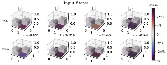
Figure 9: Output density matrices of the input state set $\mathcal{B}$ in a general superchannel $\hat{\mathcal{S}}_{g}$ scheme.

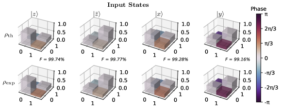
Figure 10: Output density matrices of the input state set $\mathcal{B}$ in a decomposed superchannel $\hat{\mathcal{S}}_{g}^{1}$ scheme.

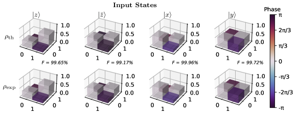
Figure 11: Output density matrices of the input state set $\mathcal{B}$ in a decomposed superchannel $\hat{\mathcal{S}}_{g}^{2}$ scheme.

Appendix B More examples of quantum superchannel

B.1 Entanglement-assisted quantum communication

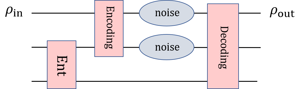
Figure 12: Circuit for entanglement-assisted quantum communication.

A notable protocol that was developed before the emerge of superchannel theory is the entanglement-assisted quantum communication entangle-com. A circuit of it is shown in Fig.12, where Ent represents the pre-existed entangled states shared by Alice and Bob. This circuit is of the form of superchannel with noise in the communication process as the input channel. The Ent and Encoding operations together form the pre-operation of the superchannel, while the decoding operation is the post-operation, which could consume additional ancillary qubits.

The entangled state $\ket{\text{Ent}}$ is used as a resource, and it is assumed to be free from noise. For instance, a common resource is the ebit, which can be generated and distributed via a specific protocol, then Alice and Bob each needs to store their qubits for the later usages. The flying qubits that will subsequently be transmitted suffer from noise, hence requiring quantum error correction. As is well known, a large class of quantum codes is the entanglement-assisted error correction codes, which possess some interesting features compared with codes without entanglement assistance Hsieh; guenda.

B.2 Noise-adapted quantum error correction

Using superchannel theory, here we show a construction of error correction codes that are noise-adapted. A common noisy channel that exists in many experimental systems is the amplitude-damping (AD) channel defined by two Kraus operators

$$K_{0}=\begin{pmatrix}1&0\\ 0&\sqrt{1-\lambda}\end{pmatrix},\;K_{1}=\begin{pmatrix}0&\sqrt{\lambda}\\ 0&0\end{pmatrix}$$ (26)

for $\lambda\in[0,1]$ as the damping parameter that encodes the evolution time. Our codes are $\gamma$-dependent and approximate, similar with some other codes in literature PhysRevA.56.2567; RN426; RN429; 4675715; Ng; MN12. In particular, we have an optimization algorithm that can find a code which can improve the quality of a noisy qubit.

Adapted to the NMR simulator we have, we use one qubit as the ancilla to generate the AD noise, and three qubits as the codes. We assume only one qubit suffers the AD noise so that we can treat our codes as distance-3 against the AD noise, approximately. Under this assumption, we theoretically consider three cases as in Fig. 13, namely, either the 1st or 2nd qubit is noisy, or with equal probability one of them is noisy, and the 3rd one, as a part of the ebit, is assumed to be noise-free.

In Fig. 14, we show the case when either one of the first two qubits is noisy. The black dashed line is the optimal result we find numerically, which is the average of the green and red lines. The fidelity is the entanglement fidelity between the error-corrected noise and a perfect identity channel. It is obvious to see when the averaged fidelity is optimal, the fidelity for merely one noise (green or red) does not need to be so, though. For each given $\gamma$, a code defined by the pair, encoding $V$ and decoding $W$ operations, is found. We can see that our codes indeed suppress the AD noise quite well, and the fidelity is high especially when $\gamma$ is small.

The primary example above shows that superchannel could be a promising framework to design error correction codes. For better and more practical codings to construct real logical qubits, we need to consider larger systems, which is left for future investigation.

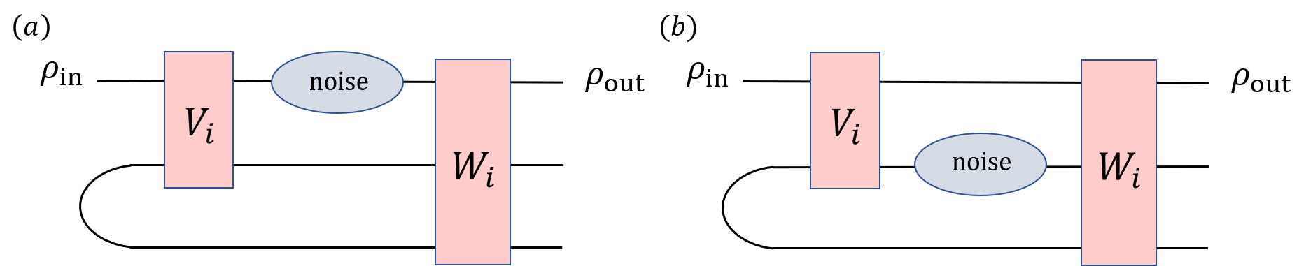
Figure 13: The ebit-assisted communication when AD noise occurs in the 1st qubit (a) and 2nd qubit (b).

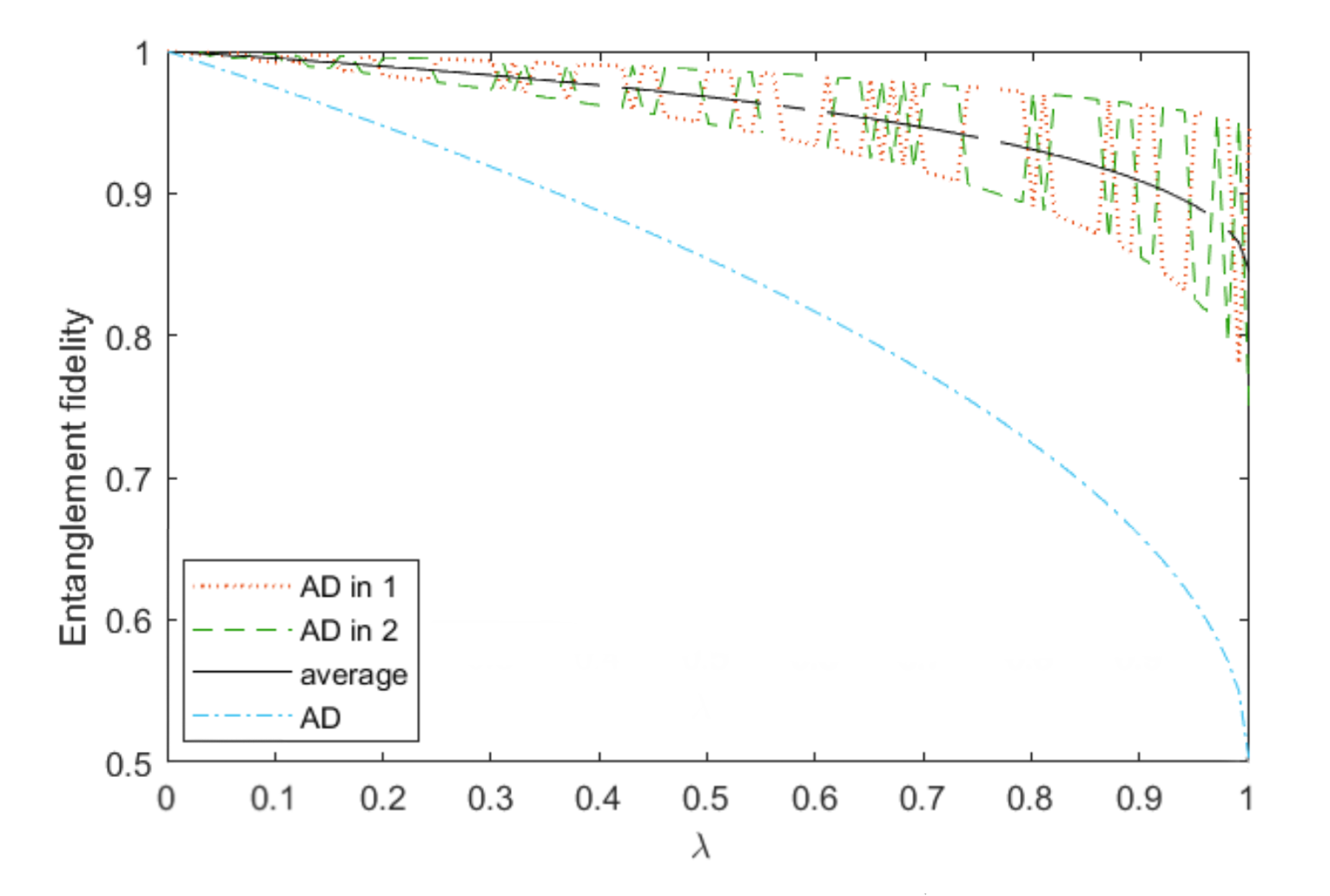
Figure 14: The entanglement fidelity with (black line) and without (blue dashed line) error correction as a function of the damping rate $\lambda$.

References

- (1) Richard P. Feynman. Simulating physics with computers. Int. J. Theor. Phys., 21(6/7):467–488, 1982.
- (2) Michael A. Nielsen and Isaac L. Chuang. Quantum Computation and Quantum Information. Cambridge University Press, Cambridge U.K., 2000.
- (3) John Preskill. Quantum computing in the NISQ era and beyond. Quantum, 2:79, 2018.
- (4) Man-Duen Choi. Completely positive linear maps on complex matrices. Linear Algebra and its Applications, 10(3):285–290, 1975.
- (5) Heinz-Peter Breuer and Francesco Petruccione. The Theory of Open Quantum System. Oxford University Press, Oxford, U.K., 2003.
- (6) Bing He, János A. Bergou, and Zhiyong Wang. Implementation of quantum operations on single-photon qudits. Phys. Rev. A, 76:042326, Oct 2007.
- (7) Marco Piani, David Pitkanen, Rainer Kaltenbaek, and Norbert Lütkenhaus. Linear-optics realization of channels for single-photon multimode qudits. Phys. Rev. A, 84:032304, Sep 2011.
- (8) D.-S. Wang, Dominic W. Berry, Marcos C. de Oliveira, and Barry C. Sanders. Solovay-Kitaev decomposition strategy for single-qubit channels. Phys. Rev. Lett., 111:130504, Sep 2013.
- (9) D.-S. Wang and Barry C. Sanders. Quantum circuit design for accurate simulation of qudit channels. New J. Phys., 14(3):033016, March 2015.
- (10) D.-S. Wang. Convex decomposition of dimension-altering quantum channels. Int. J. Quantum Inform., 14:1650045, 2016.
- (11) Ryan Sweke, Ilya Sinayskiy, and Francesco Petruccione. Simulation of single-qubit open quantum systems. Phys. Rev. A, 90:022331, Aug 2014.
- (12) Ryan Sweke, Ilya Sinayskiy, Denis Bernard, and Francesco Petruccione. Universal simulation of Markovian open quantum systems. Phys. Rev. A, 91:062308, Jun 2015.
- (13) Francesco Ticozzi and Lorenza Viola. Quantum and classical resources for unitary design of open-system evolutions. Quantum Sci. Technol., 2:034001, 2017.
- (14) W. K. Tham, H. Ferretti, A. V. Sadashivan, and A. M. Steinberg. Simulating and optimising quantum thermometry using single photons. Sci. Rep., 6:38822, 2016.
- (15) Vasco Cavina, Luca Mancino, Antonella De Pasquale, Ilaria Gianani, Marco Sbroscia, Robert I. Booth, Emanuele Roccia, Roberto Raimondi, Vittorio Giovannetti, and Marco Barbieri. Bridging thermodynamics and metrology in nonequilibrium quantum thermometry. Phys. Rev. A, 98:050101, Nov 2018.
- (16) He Lu, Chang Liu, Dong-Sheng Wang, Luo-Kan Chen, Zheng-Da Li, Xing-Can Yao, Li Li, Nai-Le Liu, Cheng-Zhi Peng, Barry C. Sanders, Yu-Ao Chen, and Jian-Wei Pan. Experimental quantum channel simulation. Phys. Rev. A, 95:042310, Apr 2017.
- (17) Tao Xin, Shi-Jie Wei, Julen S. Pedernales, Enrique Solano, and Gui-Lu Long. Quantum simulation of quantum channels in nuclear magnetic resonance. Phys. Rev. A, 96:062303, Dec 2017.
- (18) W. McCutcheon, A. McMillan, J. G. Rarity, and M. S. Tame. Experimental demonstration of a measurement-based realisation of a quantum channel. New J. Phys., 20:033019, 2018.
- (19) Ling Hu, Xianghao Mu, Weizhou Cai, Yuwei Ma, Yuan Xu, Haiyan Wang, Yipu Song, Chang-Ling Zou, and Luyan Sun. Experimental repetitive quantum channel simulation. Science Bulletin, 63(23):1551–1557, 2018.
- (20) M. H. M. Passos, A. de Oliveira Junior, M. C. de Oliveira, A. Z. Khoury, and J. A. O. Huguenin. Spin-orbit implementation of the Solovay-Kitaev decomposition of single-qubit channels. Phys. Rev. A, 102:062601, Dec 2020.
- (21) G. García-Pérez, M.A.C. Rossi, and S. Maniscalco. IBM Q experience as a versatile experimental testbed for simulating open quantum systems. npj Quantum Information, 6:1, 2020.
- (22) G. Chiribella, G. M. D’Ariano, and P. Perinotti. Transforming quantum operations: Quantum supermaps. Europhys. Lett., 83:30004, 2008.
- (23) G. Chiribella, G. M. D’Ariano, and P. Perinotti. Quantum circuit architecture. Phys. Rev. Lett., 101:060401, Aug 2008.
- (24) Giulio Chiribella, Giacomo Mauro D’Ariano, and Paolo Perinotti. Theoretical framework for quantum networks. Phys. Rev. A, 80:022339, Aug 2009.
- (25) Li Li, Michael J. W. Hall, and Howard M. Wiseman. Concepts of quantum non-Markovianity: A hierarchy. Physics Reports, 759:1–51, 2018.
- (26) Eric Chitambar and Gilad Gour. Quantum resource theories. Rev. Mod. Phys., 91:025001, Apr 2019.
- (27) Giulio Chiribella, Giacomo M. D’Ariano, and Paolo Perinotti. Memory effects in quantum channel discrimination. Phys. Rev. Lett., 101:180501, Oct 2008.
- (28) Gilad Gour. Comparison of quantum channels by superchannels. IEEE Transactions on Information Theory, 65(9):5880–5904, 2019.
- (29) Ching-Yi Lai and Todd A. Brun. Entanglement-assisted quantum error-correcting codes with imperfect ebits. Phys. Rev. A, 86:032319, Sep 2012.
- (30) Giulio Chiribella, Giacomo Mauro D’Ariano, Paolo Perinotti, and Benoit Valiron. Quantum computations without definite causal structure. Phys. Rev. A, 88:022318, Aug 2013.
- (31) Dong-Sheng Wang. Choi states, symmetry-based quantum gate teleportation, and stored-program quantum computing. Phys. Rev. A, 101:052311, May 2020.
- (32) Dong-Sheng Wang. A prototype of quantum von Neumann architecture. Communications in Theoretical Physics, 74(9):095103, Aug 2022.
- (33) Yuan-Ting Liu, Kai Wang, Yuan-Dong Liu, and Dong-Sheng Wang. A Survey of Universal Quantum von Neumann Architecture. Entropy, 25(8):1187, 2023.
- (34) Guillaume Verdon, Jason Pye, and Michael Broughton. A universal training algorithm for quantum deep learning, 2018. arXiv:quant-ph/1806.09729.
- (35) P. Mehta, M. Bukov, Ching-Hao Wang, Alexandre G. R. Day, Clint Richardson, Charles K. Fisher, and David J. Schwab. A high-bias, low-variance introduction to machine learning for physicists. Phys. Reports, 810:1–124, 2019.
- (36) Hsin-Yuan Huang, Richard Kueng, and John Preskill. Information-theoretic bounds on quantum advantage in machine learning. Phys. Rev. Lett., 126:190505, May 2021.
- (37) D.-S. Wang. A comparative study of universal quantum computing models: towards a physical unification. Quantum Engineering, 2:85, 2021.
- (38) G. J. Milburn, R. Laflamme, B. C. Sanders, and E. Knill. Quantum dynamics of two coupled qubits. Phys. Rev. A, 65:032316, Feb 2002.
- (39) L. M. K. Vandersypen and I. L. Chuang. NMR techniques for quantum control and computation. Rev. Mod. Phys., 76:1037–1069, Jan 2005.
- (40) Tao Xin, Bi-Xue Wang, Ke-Ren Li, Xiang-Yu Kong, Shi-Jie Wei, Tao Wang, Dong Ruan, and Gui-Lu Long. Nuclear magnetic resonance for quantum computing: Techniques and recent achievements. Chinese Physics B, 27(2):020308, feb 2018.
- (41) Thaddeus D Ladd, Fedor Jelezko, Raymond Laflamme, Yasunobu Nakamura, Christopher Monroe, and Jeremy Lloyd O’Brien. Quantum computers. Nature, 464(7285):45–53, 2010.
- (42) Xinhua Peng, Jingfu Zhang, Jiangfeng Du, and Dieter Suter. Quantum simulation of a system with competing two-and three-body interactions. Phys. Rev. Lett., 103(14):140501, 2009.
- (43) Dawei Lu, Hang Li, Denis-Alexandre Trottier, Jun Li, Aharon Brodutch, Anthony P Krismanich, Ahmad Ghavami, Gary I Dmitrienko, Guilu Long, Jonathan Baugh, et al. Experimental estimation of average fidelity of a Clifford gate on a 7-qubit quantum processor. Phys. Rev. Lett., 114(14):140505, 2015.
- (44) Jun Li, Ruihua Fan, Hengyan Wang, Bingtian Ye, Bei Zeng, Hui Zhai, Xinhua Peng, and Jiangfeng Du. Measuring out-of-time-order correlators on a nuclear magnetic resonance quantum simulator. Physical Review X, 7(3):031011, 2017.
- (45) Chenfeng Cao, Zheng An, Shi-Yao Hou, DL Zhou, and Bei Zeng. Quantum imaginary time evolution steered by reinforcement learning. Communications Physics, 5(1):57, 2022.
- (46) Shi-Jie Wei, Chao Wei, Peng Lv, Changpeng Shao, Pan Gao, Zengrong Zhou, Keren Li, Tao Xin, and Gui-Lu Long. A quantum algorithm for heat conduction with symmetrization. Science Bulletin, 68(5):494–502, 2023.
- (47) Nayeli A. Rodríguez-Briones, Hemant Katiyar, Eduardo Martín-Martínez, and Raymond Laflamme. Experimental activation of strong local passive states with quantum information. Phys. Rev. Lett., 130:110801, Mar 2023.
- (48) Kai Wang and Dong-Sheng Wang. Quantum circuit simulation of superchannels. New Journal of Physics, 25(4):043013, apr 2023.
- (49) Graeme Smith. Private classical capacity with a symmetric side channel and its application to quantum cryptography. Phys. Rev. A, 78:022306, Aug 2008.
- (50) Karl Kraus. States, Effects, and Operations: Fundamental Notions of Quantum Theory, volume 190 of Lecture Notes in Physics. Springer-Verlag, Berlin, 1983.
- (51) Yuchen Wang, Zixuan Hu, Barry C. Sanders, and Sabre Kais. Qudits and high-dimensional quantum computing. Front. Phys. (Lausanne), 8:589504, Nov 2020.
- (52) A Jamiołkowski. Linear transformations which preserve trace and positive semidefiniteness of operators. Rep. Math. Phys., 3:275, 1972.
- (53) Ingemar Bengtsson and Karol Zyczkowski. Geometry of Quantum States: An Introduction to Quantum Entanglement. Cambridge University Press, 2006.
- (54) G. M. D’Ariano, P. Perinotti, and M. Sedlak. Extremal quantum protocols. J. Math. Phys., 52:082202, 2011.
- (55) Mary Beth Ruskai. Open problems in quantum information theory, Aug 2007. quant-ph:0708.1902.
- (56) Mary Beth Ruskai, Stanislaw Szarek, and Elisabeth Werner. An analysis of completely-positive trace-preserving maps on M2. Linear Algebra Appl., 347(1–3):159–187, May 2002.
- (57) Navin Khaneja, Timo Reiss, Cindie Kehlet, Thomas Schulte-Herbrüggen, and Steffen J Glaser. Optimal control of coupled spin dynamics: design of NMR pulse sequences by gradient ascent algorithms. Journal of magnetic resonance, 172(2):296–305, 2005.
- (58) CA Ryan, C Negrevergne, M Laforest, Emanuel Knill, and R Laflamme. Liquid-state nuclear magnetic resonance as a testbed for developing quantum control methods. Physical Review A, 78(1):012328, 2008.
- (59) Zbigniew Puchała, Kamil Korzekwa, Roberto Salazar, Paweł Horodecki, and Karol Życzkowski. Dephasing superchannels. Phys. Rev. A, 104:052611, Nov 2021.
- (60) David G Cory, Amr F Fahmy, and Timothy F Havel. Ensemble quantum computing by NMR spectroscopy. Proceedings of the National Academy of Sciences, 94(5):1634–1639, 1997.
- (61) Mikko Möttönen, Juha J Vartiainen, Ville Bergholm, and Martti M Salomaa. Quantum circuits for general multiqubit gates. Phys. Rev. Lett., 93(13):130502, 2004.
- (62) Isaac L. Chuang and M. A. Nielsen. Prescription for experimental determination of the dynamics of a quantum black box. Journal of Modern Optics, 44(11-12):2455–2467, 1997.
- (63) Evan M Fortunato, Marco A Pravia, Nicolas Boulant, Grum Teklemariam, Timothy F Havel, and David G Cory. Design of strongly modulating pulses to implement precise effective Hamiltonians for quantum information processing. The Journal of Chemical Physics, 116(17):7599–7606, 2002.
- (64) Jingfu Zhang, Raymond Laflamme, and Dieter Suter. Experimental implementation of encoded logical qubit operations in a perfect quantum error correcting code. Phys. Rev. Lett., 109(10):100503, 2012.
- (65) Charles H. Bennett, Peter W. Shor, John A. Smolin, and Ashish V. Thapliyal. Entanglement-assisted classical capacity of noisy quantum channels. Phys. Rev. Lett., 83:3081–3084, Oct 1999.
- (66) Min-Hsiu Hsieh, Igor Devetak, and Todd Brun. General entanglement-assisted quantum error-correcting codes. Phys. Rev. A, 76:062313, Dec 2007.
- (67) Kenza Guenda, Somphong Jitman, and T Aaron Gulliver. Constructions of good entanglement-assisted quantum error correcting codes. Designs, Codes and Cryptography, 86:121–136, 2018.
- (68) Debbie W. Leung, M. A. Nielsen, Isaac L. Chuang, and Yoshihisa Yamamoto. Approximate quantum error correction can lead to better codes. Phys. Rev. A, 56:2567–2573, Oct 1997.
- (69) Andrew S. Fletcher, Peter W. Shor, and Moe Z. Win. Structured near-optimal channel-adapted quantum error correction. Physical Review A, 77(1), 2008.
- (70) Andrew S. Fletcher, Peter W. Shor, and Moe Z. Win. Optimum quantum error recovery using semidefinite programming. Physical Review A, 75(1), 2007.
- (71) Andrew S. Fletcher, Peter W. Shor, and Moe Z. Win. Channel-adapted quantum error correction for the amplitude damping channel. IEEE Transactions on Information Theory, 54(12):5705–5718, 2008.
- (72) Hui Khoon Ng and Prabha Mandayam. Simple approach to approximate quantum error correction based on the transpose channel. Phys. Rev. A, 81:062342, Jun 2010.
- (73) Prabha Mandayam and Hui Khoon Ng. Towards a unified framework for approximate quantum error correction. Phys. Rev. A, 86:012335, Jul 2012.