Identification and Estimation of Demand Models
with Endogenous Product Entry and Exit

Abstract

This paper deals with the endogeneity of firms’ entry and exit decisions in demand estimation. Product entry decisions lack a single crossing property in terms of demand unobservables, which causes the inconsistency of conventional methods dealing with selection. We present a novel and straightforward two-step approach to estimate demand while addressing endogenous product entry. In the first step, our method estimates a finite mixture model of product entry accommodating latent market types. In the second step, it estimates demand controlling for the propensity scores of all latent market types. We apply this approach to data from the airline industry.

Keywords: Demand for differentiated product; Endogenous product availability; Selection bias; Market entry and exit; Multiple equilibria; Identification; Estimation; Demand for airlines.

JEL codes: C14, C34, C35, C57, D22, L13, L93.

1 Introduction

Since the influential work by Tobin (1958), Amemiya (1973), and Heckman (1976), addressing endogenous selection has been a fundamental topic in microeconometrics. The need to handle censored observations, specifically zeros, in consumer demand estimation has made this economic application a significant driver in the development of methods to account for sample selection. While much of the early literature focused on analyzing demand for a single product, there have also been early applications to demand systems (Amemiya, 1974, Yen, 2005, Yen and Lin, 2006).

More recently, the selection problem in estimating demand systems has garnered attention within the context of structural models of demand and supply for differentiated products. A key aspect distinguishing the recently proposed methods is the source of the zeros in market shares. The first group of studies considers that the choice probabilities in the model are strictly positive, but observed market shares may be zero because they are sample means based on a small number of consumers (Gandhi, Lu, and Shi, 2023). A second approach assumes that some market shares are zero because consumers in certain markets exclude these products from their choice set or consideration set (Dubé, Hortaçsu, and Joo, 2021). Finally, a third group of studies examines sample selection bias in demand estimation when zeros arise from firms’ market entry decisions (Conlon and Mortimer, 2013, Ciliberto, Murry, and Tamer, 2021; Li, Mazur, Park, Roberts, Sweeting, and Zhang, 2022).

This paper focuses on estimating demand for differentiated products using market-level data while accounting for censoring or selection resulting from firms not offering certain products in specific markets or periods. Demand estimation typically relies on data collected from multiple geographic markets and periods, where it is common for certain products to be unavailable in specific markets or periods. When firms make their market entry decisions, they possess information about the demand for their products, particularly regarding demand components that are not observable to the researcher. Firms are more inclined to enter markets with higher expected demand. Failure to consider this selection process can introduce significant biases in the estimation of demand parameters. This issue arises across various demand applications and industries, such as the demand for airlines (Berry, Carnall, and Spiller, 2006; Berry and Jia, 2010; Aguirregabiria and Ho, 2012), supermarket chains (Smith, 2004), radio stations (Sweeting, 2013), personal computers (Eizenberg, 2014), or ice cream (Draganska, Mazzeo, and Seim, 2009).

The selection problem in this demand-entry model exhibits two key characteristics that distinguish it from more standard cases. Firstly, the non-additive nature of demand unobservables in firms’ entry decisions makes the selection function dependent not only on the entry probabilities (i.e., propensity scores) but also on all the observable variables influencing market entry. Consequently, the conventional identification results and two-step estimation methods found in the literature are not applicable (Newey, Powell, and Walker, 1990; Ahn and Powell, 1993; Powell, 2001; Das, Newey, and Vella, 2003; Aradillas-Lopez, Honoré, and Powell, 2007; Newey, 2009). Secondly, the model exhibits multiple equilibria, both in the entry game and the pricing game. Even with identical observable characteristics, different equilibria can be selected across markets. This introduces an additional source of unobserved heterogeneity that may impact sample selection.

This paper examines the identification of demand parameters within a structural model encompassing demand, price competition, and market entry, where the distribution of demand unobservables is nonparametrically specified. As in other models, the characterization of the selection problem depends crucially on the specification of firms’ information at the time of their product entry decisions. We assume that firms observe two signals on demand unobservables: a market type signal, which is common knowledge among all firms in the market and has finite support; and a private information signal, which is independent across firms. This structural framework retains the standard assumption of complete information in the Bertrand pricing game but incorporates firms’ uncertainty and private information regarding future demand, such that the product entry game is an incomplete information game. The distribution of all the unobservables in the model is nonparametric.

The paper presents three main contributions. First, it establishes the sequential (two-step) identification of demand parameters in this model. We demonstrate that the selection term in the demand equation is a convolution of the probabilities of product entry for each discrete ‘market type’ and the densities associated with these market types. Leveraging results from the literature on nonparametric finite mixture models, we show that data on firms’ product entry decisions nonparametrically identify the probabilities of product entry conditional on the market type and the density of unobserved market types. Lastly, we demonstrate that, under mild conditions on the observable variables, demand parameters are identified after effectively controlling for the nonparametric entry probabilities and densities for each market type. Our proof of sequential identification addresses two important issues in nonparametric finite mixture models: the identification up to label swapping, and the fact that sometimes we can only establish a non-binding lower bound for the number of unobserved market types.

Second, building on our constructive proof of identification, the paper proposes a simple two-step estimator to address endogenous selection. In the first step, a semiparametric mixture model is employed to estimate both the probability distribution of unobserved market types and the conditional choice probabilities of product entry in the case of a static entry game, or product entry and exit in the event of a dynamic game. In the second step, demand parameters are estimated using a Generalized Method of Moments (GMM) approach that considers both endogenous product availability and price endogeneity.

Third, the paper illustrates the proposed method by applying it to data from the airline industry. Our findings highlight the importance of accounting for endogenous product entry and for a finite mixture of latent market types, as failure to do so can lead to significant biases. Specifically, neglecting latent market types while accounting for endogenous selection results in significant attenuation biases in the estimates of demand own-price elasticities.

Our paper is motivated by and closely aligned with the work of Draganska, Mazzeo, and Seim (2009), Ciliberto, Murry, and Tamer (2021), and Li, Mazur, Park, Roberts, Sweeting, and Zhang (2022). These authors have developed methods for estimating structural models that combine the demand for differentiated products in Berry, Levinsohn, and Pakes (1995) with games of market/product entry as in Bresnahan and Reiss (1990, 1991) and Berry (1992). Their focus is on the joint estimation of all the structural parameters in the model, including demand, marginal costs, entry costs, and the probability distribution of unobservable factors. To jointly estimate the full model, these authors employ nested fixed point algorithms, which require solving multiple times for the equilibria of a two-step game. Consequently, they rely on strong parametric assumptions for all the structural functions and the distribution of unobservables. In contrast, we adopt a sequential approach to identify and estimate the structural parameters and functions within the model. Our approach yields identification outcomes that guarantee alignment of the supply side structure with an equilibrium model, all the while maintaining a nonparametric specification. This means we do not impose strong assumptions on marginal costs, entry costs, or the distribution of unobservables. Furthermore, our estimation method offers computational simplicity since it does not necessitate the computation of equilibria. Finally, the method and its computational advantages apply both to static games of market entry and dynamic games of market entry and exit.

Our model of product entry and exit relates to the literature of structural models of market entry/exit with incomplete information such as the static games in Seim (2006) and Draganska, Mazzeo, and Seim (2009) and the dynamic games in Aguirregabiria and Mira (2007), Pakes, Ostrovsky, and Berry (2007), or Sweeting (2009). The specification of the unobservables in the entry-decision part of our model — which combines common-knowledge unobservables with finite support and private information unobservables with continuous support — is closely related to the models in Xiao (2018) and Aguirregabiria and Mira (2019).

Our estimation method is rooted in and expands upon the literature on semiparametric estimation of sample selection models, with seminal contributions by Newey, Powell, and Walker (1990), Ahn and Powell (1993), Powell (2001), and Newey (2009). A distinctive aspect of our method lies in the multi-dimensionality of the selection term in the second step of estimation. Specifically, the selection term involves the convolution of functions representing market entry probabilities for each latent market type. Our method builds upon the semiparametric sieve method in Das, Newey, and Vella (2003) and Newey (2009). We enhance the applicability of this method by broadening its scope in the context of our model.

Our method also relates to the literature on estimating Conditional Average Treatment Effects (CATE) using finite mixture models for the propensity score (Haviland and Nagin, 2005, Haviland, Nagin, Rosenbaum, and Tremblay, 2008, Lanza, Coffman, and Xu, 2013). In the first step of our method, we follow a similar approach, with the only significant distinction being the crucial role played by the conditional independence between firms’ entry decisions to obtain nonparametric identification. However, the second step of our method differs substantially. Previous studies in the latent propensity score literature assign each individual in the sample to a latent class using techniques such as the highest posterior probability (modal assignment) and treating the assigned class as an observable variable. In contrast, our method recognizes that an individual’s (firm’s) latent class remains unobservable, even after estimating the finite mixture model using an infinite sample. Consequently, controlling for selection bias in the second step requires the inclusion of propensity scores for all potential latent types.

The rest of the paper is organized as follows. Section 2 presents our model and assumptions. Section 3 describes the selection problem in this model. Section 4 presents our identification results. We describe our estimation method in section 5 and illustrate it using an empirical application on the US airline industry in section 6. We summarize and conclude in section 7.

2 Model

The demand system follows the BLP framework (Berry, Levinsohn, and Pakes, 1995). For the sake of notational simplicity, we focus on single-product firms. In section 2.4, we discuss how to adapt our model and methodology to the case of multi-product firms, and more specifically the application of Lemma 1 and Assumptions 1 and 2 to this scenario. There are $J$ firms indexed by $j\in\mathcal{J}=\{1,2,...,J\}$ and $T$ markets indexed by $t\in\{1,2,...,T\}$, where a market can be a geographic location, a time period, or a combination of both. Consumers living in a market $t$ can buy only the products available in that market. Firms’ market entry decisions, prices, and quantities are determined as an equilibrium of a two-stage game. In the first stage, firms maximize their expected profit by choosing whether to be active or not in the market. In the second stage, prices and quantities of the active firms are determined as a Nash-Bertrand equilibrium of a pricing game. This two-stage game is played separately across markets. Demand and price competition are static. Our model accommodates both static and dynamic games for firms’ product entry (and exit) decisions.

2.1 Demand

The indirect utility of household $h$ in market $t$ from buying product $j$ is:

$$U_{hjt}\equiv\delta(p_{jt},\boldsymbol{x}_{jt})+v(p_{jt},\boldsymbol{x}_{jt},\upsilon_{ht})+\varepsilon_{hjt},$$ (1)

where $p_{jt}$ and $\boldsymbol{x}_{jt}$ are the price and other characteristics, respectively, of product $j$ in market $t$; $\delta_{jt}\equiv\delta(p_{jt},\boldsymbol{x}_{jt})$ is the average (indirect) utility of product $j$ in market $t$; and $v(p_{jt},\boldsymbol{x}_{jt},\upsilon_{ht})+\varepsilon_{hjt}$ represents a household-specific deviation from the average utility. The term $v(p_{jt},\boldsymbol{x}_{jt},\upsilon_{ht})$ depends on the vector of random coefficients $\upsilon_{ht}$ that is unobserved to the researcher with distribution $F_{\upsilon}(\cdot|\boldsymbol{\sigma})$, where $\boldsymbol{\sigma}$ is a vector of parameters. The term $\varepsilon_{hjt}$ is unobserved to the researcher and is i.i.d. over $(h,j,t)$ with type I extreme value distribution. Following the standard specification, the average utility of product $j$ is:

$$\delta_{jt}\equiv\alpha\text{ }p_{jt}+\boldsymbol{x}_{jt}^{\prime}\text{ }\boldsymbol{\beta}+\xi_{jt},$$ (2)

where $\alpha$ and $\boldsymbol{\beta}$ are parameters. Variable $\xi_{jt}$ captures the characteristics of product $j$ in market $t$ which are unobserved to the researcher. The outside option is represented by $j=0$ and its indirect utility is normalized to $U_{h0t}=\varepsilon_{h0t}$.

Let $a_{jt}\in\{0,1\}$ be the indicator for product $j$ being available in market $t$, and let $\boldsymbol{a}_{t}\equiv(a_{jt}:j\in\mathcal{J})$ denote the vector with the indicators for the availability of every product in market $t$. The outside option $j=0$ is always available in every market. Every household chooses the product that maximizes their utility. Let $s_{jt}$ be the market share of product $j$ in market $t$, i.e., the proportion of households choosing product $j$:

$$s_{jt}=d_{jt}(\boldsymbol{\delta}_{t},\boldsymbol{a}_{t})\equiv{\displaystyle\int}\frac{a_{jt}\text{ }\exp\left(\delta_{jt}+v(p_{jt},\boldsymbol{x}_{jt},\upsilon)\right)}{1+{\textstyle\sum\nolimits_{i=1}^{J}}a_{it}\text{ }\exp\left(\delta_{it}+v(p_{it},\boldsymbol{x}_{it},\upsilon)\right)}\text{ }dF_{\upsilon}(\upsilon).$$ (3)

This system of $J$ equations represents the demand system in market $t$. We can represent this system in a vector form as: $\boldsymbol{s}_{t}=\boldsymbol{d}_{t}(\boldsymbol{\delta}_{t},\boldsymbol{a}_{t})$.

For our analysis, it is convenient to define the sub-system of demand equations that includes market shares, average utilities, and product characteristics of only those products available in the market. We represent this system as:

$$\boldsymbol{s}_{t}^{(\boldsymbol{a})}=\boldsymbol{d}^{(\boldsymbol{a})}_{t}(\boldsymbol{\delta}_{t}^{(\boldsymbol{a})}),$$ (4)

where $\boldsymbol{s}_{t}^{(\boldsymbol{a})}$ is the subvector of $\boldsymbol{s}_{t}$ containing the market shares for only those products available in the market and a similar definition applies to the subvector $\boldsymbol{\delta}^{(\boldsymbol{a})}_{t}$. Lemma 1 establishes that the invertibility property in Berry (1994) applies to demand system (4) for any value of $\boldsymbol{a}$.

LEMMA 1. Suppose that the outside option $j=0$ is always available. Then, for any value of the vector $\boldsymbol{a}\in\{0,1\}^{J}$, the system $\boldsymbol{s}_{t}^{(\boldsymbol{a})}=\boldsymbol{d}^{(\boldsymbol{a})}_{t}(\boldsymbol{\delta}_{t}^{(\boldsymbol{a})})$ is invertible with respect to $\boldsymbol{\delta}_{t}^{(\boldsymbol{a})}$ such that for every product in this subsystem (i.e., for every product with $a_{jt}=1$) the inverse function $\delta_{jt}^{(\boldsymbol{a})}=d_{jt}^{-1}(\boldsymbol{s}_{t}^{(\boldsymbol{a})})$ exists.   $\blacksquare$

Proof of Lemma 1. If the outside option $j=0$ is available, then, for any value of the vector $\boldsymbol{a}$, the system of equations (4) satisfies the conditions for invertibility in Berry (1994).   $\blacksquare$

For a product available in market $t$, we have:

$$d_{jt}^{-1}(\boldsymbol{s}_{t}^{(\boldsymbol{a}_{t})})\text{ }=\text{ }\delta_{jt}\text{ }=\text{ }\alpha\text{ }p_{jt}+\boldsymbol{x}_{jt}^{\prime}\text{ }\boldsymbol{\beta}+\xi_{jt}\text{ \ \ if and only if \ \ }a_{jt}=1.$$ (5)

Importantly, this regression equation for product $j$ only depends on the availability of product $j$ and not on the availability of the other products. Therefore, the selection problem in the estimation of the demand of product $j$ can be described in terms of the conditional expectation

$$\mathbb{E}\left(\xi_{jt}\text{ }|\text{ }a_{jt}=1\right).$$ (6)

This is an important implication of working directly with the inverse demand system, as represented by equation (5).

To appreciate the value of this property, consider instead the case of the Almost Ideal Demand System (AIDS) (Deaton and Muellbauer, 1980). In the AIDS, each value of the vector $\boldsymbol{a}_{t}$ implies a different set of regressors and slope parameters in the regression equation that relates the demand of product $j$ to the log-prices of the available products. Therefore, in the AIDS model, the selection problem in the estimation of the demand of product $j$ is not only related to the availability of that product but to the availability of all products in the system. In other words, the selection term cannot be represented in terms of $\mathbb{E}\left(\xi_{jt}\text{ }|\text{ }a_{jt}=1\right)$ but must instead be expressed in terms of $\mathbb{E}\left(\xi_{jt}\text{ }|\text{ }a_{jt}=1,\text{ }\boldsymbol{a}_{-jt}=\boldsymbol{a}_{-j}\right)$. That is, in the AIDS model we have a different selection term for each value of the vector $\boldsymbol{a}_{-j}$ representing the availability of products other than $j$. This structure makes the selection problem multi-dimensional and significantly complicates identification and estimation when the number of products $J$ is large.

The next Example illustrates Lemma 1 in the case of a nested logit model.

EXAMPLE 1 (Nested logit model).

The $J$ products are partitioned into $R$ mutually exclusive groups indexed by $r$. We denote by $r_{j}$ the group to which product $j$ belongs. The indirect utility function is $U_{htj}\equiv\delta_{jt}+(1-\sigma)\text{ }v_{ht,r_{j}}+\varepsilon_{htj}$, where variables $v$ and $\varepsilon$ are independently distributed, $\varepsilon$ and $(1-\sigma)\text{ }v+\varepsilon$ are i.i.d. type I extreme value, and $\sigma\in[0,1]$ is a parameter (Cardell, 1997). This model implies $s_{jt}=d_{j}^{(\boldsymbol{a}_{t})}(\boldsymbol{\delta}_{t})=$ $d_{r_{j}}^{(\boldsymbol{a}_{t})}$ $d_{j|r_{j}}^{(\boldsymbol{a}_{t})}$ with

$$d_{j|r_{j}}^{(\boldsymbol{a}_{t})}=\frac{a_{jt}\text{ }e^{\delta_{jt}}}{{\textstyle\sum\nolimits_{i\in r_{j}}}a_{it}\text{ }e^{\delta_{it}}}\text{ \ and \ }d_{r_{j}}^{(\boldsymbol{a}_{t})}=\frac{\left[{\textstyle\sum\nolimits_{i\in r_{j}}}a_{it}\text{ }e^{\delta_{it}}\right]^{\tfrac{1}{1-\sigma}}}{1+{\textstyle\sum\nolimits_{r=1}^{R}}\left[{\textstyle\sum\nolimits_{i\in r}}a_{it}\text{ }e^{\delta_{it}}\right]^{\tfrac{1}{1-\sigma}.}}$$ (7)

If $a_{jt}=1$ and $s_{0t}>0$, the inverse function $d_{j}^{(\boldsymbol{a}_{t})-1}(\cdot)$ exists — regardless of the value of $a_{it}$ for any product $i$ different from $j$. It is straightforward to show that this inverse function has the following form:

$$\delta_{jt}=\ln\left(\frac{s_{jt}}{s_{0t}}\right)-\sigma\text{ }\ln\left(\frac{{\textstyle\sum\nolimits_{i\in r_{j}}}s_{it}}{s_{0t}}\right)$$ (8)

and it implies the regression equation:

$$\ln\left(\frac{s_{jt}}{s_{0t}}\right)=\sigma\text{ }\ln\left(\frac{{\textstyle\sum\nolimits_{i\in r_{j}}}s_{it}}{s_{0t}}\right)+\alpha\text{ }p_{jt}+\boldsymbol{x}_{jt}^{\prime}\text{ }\boldsymbol{\beta}+\xi_{jt}.$$ (9)

Given $s_{0t}>0$, this regression equation holds whenever $a_{jt}=1$.   $\blacksquare$

2.2 Price competition

Let $\Pi_{jt}$ be the profit of firm $j$ if active in market $t$. This equals revenues minus costs:

$$\Pi_{jt}=p_{jt}\text{ }q_{jt}-c(q_{jt};\boldsymbol{x}_{jt},\omega_{jt})-f(\boldsymbol{x}_{jt},\eta_{jt}),$$ (10)

where $q_{jt}$ is the quantity sold (i.e., market share $s_{jt}$ times market size $H_{t}$), $c(q_{jt};\boldsymbol{x}_{jt},\omega_{jt})$ is the variable cost function, and $f(\boldsymbol{x}_{jt},\eta_{jt})$ is the fixed entry cost. Variables $\omega_{jt}$ and $\eta_{jt}$ are unobserved to the researcher.

Given firms’ entry decisions, the best response function in the Bertrand pricing game implies the following system of pricing equations:

$$p_{jt}=mc_{jt}-d_{jt}^{(\boldsymbol{a}_{t})}\text{ }\left[\dfrac{\partial d_{jt}^{(\boldsymbol{a}_{t})}}{\partial p_{jt}}\right]^{-1}\text{ for every }j\in\mathcal{J},$$ (11)

where $mc_{jt}$ is the marginal cost $\partial c_{jt}/\partial q_{jt}$. A solution to this system of equations is a Nash-Bertrand equilibrium. The pricing game may have multiple equilibria. We do not impose restrictions on equilibrium selection and allow each market to potentially select a different equilibrium. We use scalar variable $\tau^{2}_{t}$ to index the equilibrium type selected in the Bertrand game, i.e., in step 2 of the two-stage game.

Let $\boldsymbol{x}_{t}\equiv(\boldsymbol{x}_{jt}:j\in\mathcal{J})$ be the vector with all the exogenous variables that are observed to the researcher, affecting demand or costs. Vectors $\boldsymbol{\xi}_{t}$ and $\boldsymbol{\omega}_{t}$ have similar definitions. Let $\boldsymbol{a}_{-jt}$ be the vector with the entry decisions of every firm other than $j$. We use $VP_{j}(\boldsymbol{a}_{-jt},\boldsymbol{x}_{t},\boldsymbol{\xi}_{t},\boldsymbol{\omega}_{t},\tau^{2}_{t})$ to denote the indirect variable profit function for firm $j$ that results from plugging into the expression $p_{jt}$ $q_{jt}-c(q_{jt};\boldsymbol{x}_{jt},\omega_{jt})$ the value of $(p_{jt},q_{jt})$ from the Nash-Bertrand equilibrium given $(a_{jt}=1,\boldsymbol{a}_{-jt},\boldsymbol{x}_{t},\boldsymbol{\xi}_{t},\boldsymbol{\omega}_{t},\tau^{2}_{t})$.

2.3 Market entry game and information structure

Firms’ entry decisions are determined as an equilibrium of a game of market entry. The profit of being inactive is normalized to zero for all firms. Firms have uncertainty about their profits if active in the market. Their information about demand and costs plays a key role in their entry decisions and, therefore, on the selection problem in the estimation of demand. Assumptions 1 and 2 summarize our conditions on the information structure and on the entry cost function, respectively.

ASSUMPTION 1. Firm $j$’s information at the moment of its entry decision in market $t$ consists of $(\boldsymbol{x}_{t},\kappa_{t},\tau^{1}_{t},\eta_{jt})$.

• $\kappa_{t}$ is a signal for the demand-cost variables $(\boldsymbol{\xi}_{t},\boldsymbol{\omega}_{t},\tau^{2}_{t})$. It is common knowledge for the firms, it has discrete and finite support that we denote as $\mathcal{K}(\boldsymbol{x}_{t})$, and its probability distribution conditional on $\boldsymbol{x}_{t}$ is $f_{\kappa}(\kappa_{t}|\boldsymbol{x}_{t})$, which is nonparametrically specified.

• Variable $\tau^{1}_{t}$ represents the type of equilibrium selected in the entry game.

• Variable $\eta_{jt}$ is a component of the entry cost that is private information of firm $j$, independently distributed over firms, and independent of $(\kappa_{t},\boldsymbol{x}_{t})$ with CDF $F_{\eta}$, which is strictly increasing over the real line.

• Vector $(\boldsymbol{\xi}_{t},\boldsymbol{\omega}_{t},\tau^{2}_{t},\kappa_{t},\tau^{1}_{t},\eta_{jt})$ is unobserved to the researcher. Conditional on $\kappa_{t}$, variables $\boldsymbol{\xi}_{t}$, $\boldsymbol{\omega}_{t}$, and $\eta_{jt}$ are independent of $\boldsymbol{x}_{t}$.   $\blacksquare$

For our analysis, the payoff-relevant information in discrete variable $\kappa_{t}$ plays the same role as the equilibrium-selection discrete variable $\tau^{1}_{t}$. Therefore, for notational simplicity, we omit $\tau^{1}_{t}$ and interpret $\kappa_{t}$ as representing both equilibrium selection and payoff relevant variables. Let $|\mathcal{K}(\boldsymbol{x}_{t})|$ be the number of points in the support of $\kappa_{t}$. We then represent $\kappa_{t}$ as an index with support $\{1,2,...,|\mathcal{K}(\boldsymbol{x}_{t})|\}$. Similarly, with some abuse of notation, for the rest of the paper we represent the vector of unobservables $(\boldsymbol{\xi}_{t},\boldsymbol{\omega}_{t},\tau^{2}_{t})$ using the more compact notation $\boldsymbol{\xi}_{t}$.

Let $\pi_{j}(\boldsymbol{a}_{-j},\boldsymbol{x}_{t},\kappa_{t},\eta_{jt})$ be firm $j$’s expected profit given its information about demand and costs and conditional on the hypothetical entry profile $\boldsymbol{a}_{-j}\in\{0,1\}^{J-1}$. Under Assumption 1:

$$\pi_{j}(\boldsymbol{a}_{-j},\boldsymbol{x}_{t},\kappa_{t},\eta_{jt})\text{ }=\text{ }{\displaystyle\int}VP_{j}(\boldsymbol{a}_{-j},\boldsymbol{x}_{t},\boldsymbol{\xi}_{t})\text{ }dF_{j,\xi}\left(\boldsymbol{\xi}_{t}\text{ }|\text{ }\kappa_{t},\eta_{jt}\right)-f(\boldsymbol{x}_{jt},\eta_{jt}),$$ (12)

where $F_{j,\xi}\left(\boldsymbol{\xi}_{t}\text{ }|\text{ }\kappa_{t},\eta_{jt}\right)$ is the CDF of $\boldsymbol{\xi}_{t}$ conditional on $(\kappa_{t},\eta_{jt})$.

ASSUMPTION 2. For any value $(\boldsymbol{a}_{-j},\boldsymbol{x}_{t},\kappa_{t})$, the function $\pi_{j}(\boldsymbol{a}_{-j},\boldsymbol{x}_{t},\kappa_{t},\eta_{jt})$ is strictly monotonic in $\eta_{jt}$. Without loss of generality, we consider that this function is decreasing in $\eta_{jt}$. Therefore, for any scalar value $\pi^{0}$ and any value $(\boldsymbol{a}_{-j},\boldsymbol{x}_{t},\kappa_{t})$, the equation $\pi^{0}=\pi_{j}(\boldsymbol{a}_{-j},\boldsymbol{x}_{t},\kappa_{t},\eta_{jt})$ is invertible with respect to $\eta_{jt}$. That is, there is an inverse function $\pi_{j}^{-1}$ such that $\eta_{jt}=\pi_{j}^{-1}(\boldsymbol{a}_{-j},\boldsymbol{x}_{t},\kappa_{t},\pi^{0})$, and for any other scalar $\pi^{1}$ with $\pi^{1}\leq\pi^{0}$, we have that $\pi_{j}^{-1}(\boldsymbol{a}_{-j},\boldsymbol{x}_{t},\kappa_{t},\pi^{1})\geq\eta_{jt}$.   $\blacksquare$

The presence of firms’ private information implies that the entry game is of incomplete information. Given $(\boldsymbol{x}_{t},\kappa_{t})$, a Bayesian Nash Equilibrium (BNE) of this game can be represented as a $J$-tuple of entry probabilities, one for each firm, $(P_{jt}:j\in\mathcal{J)}$. To describe this BNE, we first define a firm’s expected profit function that accounts for its uncertainty about other firms’ entry decisions.

$$\pi_{j}^{P}(\boldsymbol{x}_{t},\kappa_{t},\eta_{jt})=\sum_{\boldsymbol{a}_{-j}\in\{0,1\}^{J-1}}\left({\displaystyle\prod\limits_{i\neq j}}\left[P_{it}\right]^{a_{i}}\left[1-P_{it}\right]^{1-a_{i}}\right)\pi_{j}(\boldsymbol{a}_{-j},\boldsymbol{x}_{t},\kappa_{t},\eta_{jt}).$$ (13)

Under Assumption 2, the expected profit function $\pi_{j}^{P}(\boldsymbol{x}_{t},\kappa_{t},\eta_{jt})$ is strictly monotonic and invertible in $\eta_{jt}$. Let $\pi_{j}^{P(-1)}$ be this inverse function. Then, given the entry probabilities of its competitors, firm $j$’s best response is to enter in the market if and only if:

$$\eta_{jt}\text{ }\leq\text{ }\pi_{j}^{P(-1)}(\boldsymbol{x}_{t},\kappa_{t},0)$$ (14)

Taking this into account, we can define a BNE in this game as follows.

DEFINITION 1 (BNE). Under Assumptions 1-2 and given $(\boldsymbol{x}_{t},\kappa_{t})$, a Bayesian Nash Equilibrium (BNE) can be represented as a $J$-tuple of probabilities $\{P_{jt}\equiv P_{j}(\boldsymbol{x}_{t},\kappa_{t}):j\in\mathcal{J)}\}$ that solve the following system of $J$ best response equations in the space of probabilities:

$$P_{jt}\text{ }=\text{ }F_{\eta}\left(\pi_{j}^{P(-1)}\left(\boldsymbol{x}_{t},\kappa_{t},0\right)\right),$$ (15)

where $\pi_{j}^{P(-1)}$ is the inverse function with respect to $\eta_{jt}$ of the expected profit in (13).   $\blacksquare$

This framework encompasses various information structures concerning the unobservable factors, all corresponding to distinct scenarios considered within structural models of market entry and product introduction. When Var$(\kappa_{t})=0$, the scenario aligns with an entry game featuring solely private information unobservables, as examined in studies such as Seim (2006), Sweeting (2009), and Bajari, Hong, Krainer, and Nekipelov (2010). As Var$(\eta_{jt})$ approaches zero, we converge to a scenario characterized by an entry game involving exclusively complete information unobservables, as in the work by Ciliberto and Tamer (2009) and Ciliberto, Murry, and Tamer (2021). In instances where Var$(\kappa_{t})>0$ and Var$(\eta_{jt})>0$, the model describes an entry game encompassing both categories of unobservable factors, as in the work by Grieco (2014) and Aguirregabiria and Mira (2019).

2.4 Multi-product firms

We briefly discuss here how the model, the results above, and the characterization of the selection problem in section 3 below can be extended to the case of multi-product firms. We still use $j\in\mathcal{J}$ to index products but now we introduce the firm sub-index $f$ and define $\mathcal{J}_{f}\subseteq\mathcal{J}$ as the set of products owned by firm $f$. The product entry decisions of firm $f$ are described by vector $\boldsymbol{a}_{ft}\equiv(a_{jt}:j\in\mathcal{J}_{f})\in\{0,1\}^{|\mathcal{J}_{f}|}$.

First, it is important to note that Lemma 1’s applicability remains unaffected by the product ownership structure. This Lemma only rests on the structure of the demand system. Therefore, regardless of the product ownership structure, the selection problem in the estimation of the demand of product $j$ is still described in terms of the conditional expectation $\mathbb{E}\left(\xi_{jt}\text{ }|\text{ }a_{jt}=1\right)$.

Second, Assumption 1, which describes a firm’s information at the moment of its entry decisions in a market $t$, remains basically the same when we consider multi-product firms. The only difference is that we need to represent a firm’s private information entry cost using a vector with as many elements as possible products for this firm; that is, $\boldsymbol{\eta}_{ft}\equiv(\eta_{ft}(\boldsymbol{a}_{f}):\boldsymbol{a}_{f}\in\{0,1\}^{|\mathcal{J}_{f}|})$. For instance, in the case of a two-product firm, $\eta_{ft}(1,0)$ is the latent component of entry cost when the firm offers product 1 while excluding product 2. Under Assumption 1, equation (12), describing the expected profit of a firm, readily extends to multi-product firms as follows:

$$\pi_{f}\left(\boldsymbol{a}_{f},\boldsymbol{a}_{-f},\boldsymbol{x}_{t},\kappa_{t},\boldsymbol{\eta}_{ft}\right)\text{ }=\text{ }{\displaystyle\int}VP_{f}\left(\boldsymbol{a}_{f},\boldsymbol{a}_{-f},\boldsymbol{x}_{t},\boldsymbol{\xi}_{t}\right)\text{ }dF_{f,\xi}\left(\boldsymbol{\xi}_{t}\text{ }|\text{ }\kappa_{t},\boldsymbol{\eta}_{ft}\right)-f(\boldsymbol{x}_{ft},\boldsymbol{\eta}_{ft}),$$ (16)

where $F_{f,\xi}\left(\boldsymbol{\xi}_{t}\text{ }|\text{ }\kappa_{t},\boldsymbol{\eta}_{ft}\right)$ is the CDF of $\boldsymbol{\xi}_{t}$ conditional on $(\kappa_{t},\boldsymbol{\eta}_{ft})$.

The following Assumption 2-Multi is the extension of Assumption 2 to the case of multi-product firms.

ASSUMPTION 2-Multi. The expected profit function $\pi_{f}$ has a structure with respect to $\boldsymbol{\eta}_{ft}$ implying that a choice of product portfolio maximizes expected profit if and only if the elements in vector $\boldsymbol{\eta}_{ft}$ satisfy $|\mathcal{J}_{f}|-1$ thresholds conditions, where the threshold values are functions only of $(\boldsymbol{x}_{t},\kappa_{t})$, say, $\boldsymbol{g}_{f}(\boldsymbol{x}_{t},\kappa_{t})$. For instance $\boldsymbol{a}_{ft}=\boldsymbol{a}_{f}$ if and only if $\boldsymbol{\eta}_{ft}\leq\boldsymbol{g}_{f}(\boldsymbol{x}_{t},\kappa_{t})$.   $\blacksquare$

Under Assumption 2-Multi, the probability of choosing a product portfolio is a function of the vector of thresholds $\boldsymbol{g}_{f}(\boldsymbol{x}_{t},\kappa_{t})$. There is a one-to-one relationship between the $|\mathcal{J}_{f}|-1$ dimension vector of portfolio-choice probabilities and the vector of threshold values. This structure implies that the characterization of the selection term in the demand regression model is similar with multi-product or single-product firms. In section 3 below, for single-product firms, we show that this selection term is the average over all possible unobserved market types $\kappa_{t}$ of a function of the product entry probability $P_{j}(\boldsymbol{x}_{t},\kappa_{t})$. Similarly, in the multi-product case, the selection term is the average over all possible unobserved market types of a function of the vector of probabilities of every possible product portfolio.

While the preceding discussion illustrates the similar structure shared by the selection problem with single- and multi-product firms, it also underscores a noteworthy practical difference. The dimension of the vector of choice probabilities we need to control for to deal with sample selection bias grows exponentially with the number of products per firm. In some applications, this can pose a substantial challenge in the practical implementation of our method.

2.5 Dynamic game of product entry and exit

Our framework and identification results can accommodate cases in which firms’ decisions about product availability come from a Markov Perfect Equilibrium (MPE) of a dynamic game of product entry and exit, where firms are forward-looking. In this dynamic game, a firm’s fixed cost is denoted as $f(a_{it},a_{i,t-1},\boldsymbol{x}_{jt},\eta_{jt})$, where $f(1,0,\boldsymbol{x}_{jt},\eta_{jt})$ represents the cost of entry, $f(0,1,\boldsymbol{x}_{jt},\eta_{jt})$ is the cost of exit, $f(1,1,\boldsymbol{x}_{jt},\eta_{jt})$ is the fixed cost when a product stays in the market, and $f(0,0,\boldsymbol{x}_{jt},\eta_{jt})$ can be normalized to zero.

ASSUMPTION 3. Suppose that $t$ represents time. (A) The vector of state variables at period $t$, $\boldsymbol{x}_{t}$, includes the entry decisions of all the firms at the previous period, $(a_{j,t-1}:j=1,2,...,J)$. (B) The exogenous product characteristics in vector $\boldsymbol{x}_{t}$ and the latent market type $\kappa_{t}$ are either time-invariant or follow a first-order Markov process. (C) The private information shock $\eta_{jt}$ is independently and identically distributed over time and independent across firms.   $\blacksquare$

Assumptions 3(B) and 3(C) are standard in the literature of empirical dynamic discrete choice games (see Aguirregabiria, Collard-Wexler, and Ryan, 2021). Under Assumption 3, the value of being or not in the market depends on the state variables $(\boldsymbol{x}_{t},\kappa_{t})$ and on the private information shock $\eta_{jt}$. Let $v^{P}_{j}(\boldsymbol{x}_{t},\kappa_{t},\eta_{jt})$ be the difference between the value functions of being in the market and not being in the market at period $t$. This function can be represented as the sum of two functions: the difference between current profits and the difference between expected continuation values. Assumption 3(C) implies that $\eta_{jt}$ enters in the current profit but not in the expected continuation value. Therefore, by Assumption 2 on the strict monotonicity of the profit function with respect to $\eta_{jt}$, we have that the value function $v^{P}_{j}(\boldsymbol{x}_{t},\kappa_{t},\eta_{jt})$ is also strictly monotonic in $\eta_{jt}$. This implies that the best response of a firm in the dynamic game can be described by a threshold condition as in equation (14). Consequently, and similar to a BNE in a static entry game, a MPE in a dynamic game can be characterized in terms of $J$ conditional choice probabilities.

DEFINITION 2 (MPE). Suppose that Assumptions 1-3 hold. Then, a Markov Perfect Equilibrium (MPE) can be represented as a $J$-tuple of probability functions $\{P_{j}(\boldsymbol{x}_{t},\kappa_{t}):j\in\mathcal{J)}\}$ that solve the following system of best response equations in the space of probability functions:

$$P_{j}\left(\boldsymbol{x}_{t},\kappa_{t}\right)\text{ }=\text{ }F_{\eta}\left(v_{j}^{P(-1)}\left(\boldsymbol{x}_{t},\kappa_{t},0\right)\right),$$ (17)

where $v_{j}^{P(-1)}$ is the inverse function with respect to $\eta_{jt}$ of the difference between the value of being in the market and the value of not being in the market at period $t$.   $\blacksquare$

For the rest of the paper, we will not distinguish whether the choice probabilities $P_{j}\left(\boldsymbol{x}_{t},\kappa_{t}\right)$ come from a BNE of a static entry game or from a MPE of a dynamic entry/exit game. All our identification results apply to both cases.

3 Selection problem

For simplicity and concreteness, we describe our sample selection problem using the nested logit demand model from Example 1. We use the starred variables $s_{jt}^{\ast}$ and $p_{jt}^{\ast}$ to represent latent variables. That is, $s_{jt}^{\ast}$ and $p_{jt}^{\ast}$ represent the latent market share and price, respectively, that we would observe if product $j$ were offered in market $t$. Using these latent variables, we can write the following demand system:

$$\ln\left(\frac{s_{jt}^{\ast}}{s_{0t}}\right)\text{ }=\text{ }\sigma\text{ }\ln\left(\frac{s_{jt}^{\ast}+S_{-jt}}{s_{0t}}\right)+\alpha\text{ }p_{jt}^{\ast}+\boldsymbol{x}_{jt}^{\prime}\text{ }\boldsymbol{\beta}+\xi_{jt}\text{,}$$ (18)

where $S_{-jt}\equiv{\textstyle\sum\nolimits_{i\neq j,i\in r_{j}}}s_{it}$ is the aggregate market share of all products in group $r_{j}$ other than product $j$. Latent variables $(s_{jt}^{\ast},p_{jt}^{\ast})$ are equal to the observed variables $(s_{jt},p_{jt})$ if and only if product $j$ is offered in market $t$:

$$\{s_{jt}^{\ast}=s_{jt}\text{ and }p_{jt}^{\ast}=p_{jt}\}\text{ if and only if }a_{jt}=1.$$ (19)

Firm $j$’s best response entry decision completes the econometric model:

$$a_{jt}\text{ }=\text{ }1\left\{\eta_{jt}\text{ }\leq\text{ }\pi_{j}^{P(-1)}(\boldsymbol{x}_{t},\kappa_{t})\right\}.$$ (20)

Equations (18) to (20) imply the following regression equation for any product with $a_{jt}=1$:

$$\ln\left(\frac{s_{jt}}{s_{0t}}\right)\text{ }=\text{ }\sigma\text{ }\ln\left(\frac{s_{jt}+S_{-jt}}{s_{0t}}\right)+\alpha\text{ }p_{jt}+\boldsymbol{x}_{jt}^{\prime}\text{ }\boldsymbol{\beta}+\lambda_{j}(\boldsymbol{x}_{t})+\widetilde{\xi}_{jt}\text{,}$$ (21)

where $\lambda_{j}(\boldsymbol{x}_{t})$ is the selection bias function, $\mathbb{E}\left(\xi_{jt}\text{ }|\text{ }\boldsymbol{x}_{t},a_{jt}=1\right)$. That is,

$$\lambda_{j}(\boldsymbol{x}_{t})={\displaystyle\int}\xi_{jt}\text{ }1\left\{\eta_{jt}\text{ }\leq\text{ }\pi_{j}^{P(-1)}(\boldsymbol{x}_{t},\kappa_{t})\right\}\text{ }\dfrac{f_{\xi,\eta,\kappa}\left(\xi_{jt},\eta_{jt},\kappa_{t}|\boldsymbol{x}_{t}\right)}{\Pr\left(a_{jt}=1|\boldsymbol{x}_{t}\right)}\text{ }d\left(\xi_{jt}\text{,}\eta_{jt},\kappa_{t}\right),$$ (22)

and:

$$\Pr\left(a_{jt}=1|\boldsymbol{x}_{t}\right)\equiv\mathbb{E}\left(a_{jt}\text{ }|\text{ }\boldsymbol{x}_{t}\right)={\displaystyle\int}1\left\{\eta_{jt}\text{ }\leq\text{ }\pi_{j}^{P(-1)}(\boldsymbol{x}_{t},\kappa_{t})\right\}\text{ }f_{\eta,\kappa}\left(\eta_{jt},\kappa_{t}|\boldsymbol{x}_{t}\right)\text{ }d\left(\eta_{jt},\kappa_{t}\right),$$ (23)

where $f_{\eta,\kappa}$ and $f_{\xi,\eta,\kappa}$ are the joint density functions of $\left(\eta_{jt},\kappa_{t}\right)$ and $\left(\xi_{jt}\text{,}\eta_{jt},\kappa_{t}\right)$, conditional of $\boldsymbol{x}_{t}$, respectively.

Note that the selection bias function $\lambda_{j}(\boldsymbol{x}_{t})$ is a nonparametric function of all its arguments $\boldsymbol{x}_{t}$. Therefore, based on equation (21), and without further restrictions, the demand parameters $\sigma$, $\alpha$, and $\boldsymbol{\beta}$ are not identified. That is, we cannot disentangle the direct effect of $\boldsymbol{x}_{jt}$ on demand (as represented by the vector of parameters $\boldsymbol{\beta}$) from the indirect effect that comes from the selection bias function $\lambda_{j}(\boldsymbol{x}_{t})$.

Examples 2 and 3 below present restrictions that imply the identification of the demand parameters. Example 2 is simple but it imposes strong restrictions on the unobservables. Our main identification results in section 4 are closely related to Example 3.

EXAMPLE 2 (No signals $\kappa_{t}$).

Suppose that: (1^∗) $\kappa_{t}=0$ such that, at the moment of the entry decision, the only information that a firm has about the demand/cost variables $\boldsymbol{\xi}_{t}$ is its private information variable $\eta_{jt}$; and (2^∗) a unique equilibrium is played across all entry games with the same observables $\boldsymbol{x}_{t}$. Under conditions (1^∗) and (2^∗), the selection term $\lambda_{j}(\boldsymbol{x}_{t})$ only depends on the CCP $P_{j}\left(\boldsymbol{x}_{t}\right)$: that is, $\lambda_{j}(\boldsymbol{x}_{t})=\rho_{j}(P_{j}\left(\boldsymbol{x}_{t}\right))$ for some function $\rho_{j}(\cdot)$.

The proof is straightforward. Under conditions (1^∗)-(2^∗), the inverse profit function $\pi_{j}^{P(-1)}$ and the equilibrium entry probability $P_{j}$ only depend on $\boldsymbol{x}_{t}$ but not on $\kappa_{t}$. The equilibrium entry probability $P_{j}\left(\boldsymbol{x}_{t}\right)$ is equal to the conditional expectation $\mathbb{E}\left(a_{jt}|\boldsymbol{x}_{t}\right)$, which is nonparametrically identified. Furthermore, this probability satisfies the equilibrium condition $P_{j}(\boldsymbol{x}_{t})$ $=$ $F_{\eta}(\pi_{j}^{P(-1)}(\boldsymbol{x}_{t}))$, such that $\pi_{j}^{P(-1)}(\boldsymbol{x}_{t})=$ $F_{\eta}^{-1}(P_{j}(\boldsymbol{x}_{t}))$, and the entry condition can be represented as $a_{jt}=1\{\eta_{jt}\leq F_{\eta}^{-1}(P_{j}(\boldsymbol{x}_{t}))\}$. Independence between $(\xi_{jt},\eta_{jt})$ and $\boldsymbol{x}_{t}$ then implies that:

$$\lambda_{j}(\boldsymbol{x}_{t})\text{ }=\text{ }{\displaystyle\int}\xi_{jt}\text{ }1\left\{\eta_{jt}\leq F_{\eta}^{-1}(P_{j}\left(\boldsymbol{x}_{t}\right))\right\}\text{ }\dfrac{f_{\xi,\eta}\left(\xi_{jt},\eta_{jt}\right)}{P_{j}\left(\boldsymbol{x}_{t}\right)}\text{ }d\xi_{jt}\text{ }d\eta_{jt}\text{ }=\text{ }\rho_{j}(P_{j}\left(\boldsymbol{x}_{t}\right))$$ (24)

Therefore, the demand equation can be represented as:

$$\ln\left(\frac{s_{jt}}{s_{0t}}\right)=\sigma\text{ }\ln\left(\frac{s_{jt}+S_{-jt}}{s_{0t}}\right)+\alpha\text{ }p_{jt}+\boldsymbol{x}_{jt}^{\prime}\text{ }\boldsymbol{\beta}+\rho_{j}(P_{j}\left(\boldsymbol{x}_{t}\right))+\widetilde{\xi}_{jt}.$$ (25)

The result in equation (25) has important implications for identification and estimation. Regression equation (25) is a standard semiparametric partially linear model with two endogenous regressors, $\ln[(s_{jt}+S_{-jt})/s_{0t}]$ and $p_{jt}$, and with the nonparametric component $\rho_{j}(P_{j}\left(\boldsymbol{x}_{t}\right))$ only depending on the CCP of firm $j$. As such, identification and estimation follows a standard two-step procedure. In a first step, we nonparametrically estimate $P_{j}\left(\boldsymbol{x}_{t}\right)$ from data on $(a_{jt},\boldsymbol{x}_{t})$. Then, in a second step, one can apply the semiparametric series estimator in Das, Newey, and Vella (2003) and Newey (2009), or the pairwise differencing method in Powell (2001) and Aradillas-Lopez (2012). Valid instruments in this regression are observed $\boldsymbol{x}$ characteristics of products other than $j$, i.e., the so-called BLP instruments. $\qquad\blacksquare$

Under the assumptions of Example 2, the market entry condition has only one unobservable variable, $\eta_{jt}$, which, after inverting the profit function, enters additively in the inequality that defines the selection/entry decision. The model becomes a standard semiparametric sample selection model. However, though practically convenient, the conditions in Example 2 are likely to be rejected in many empirical applications. In particular, restriction (1^∗) — i.e., $\eta_{jt}$ is the only relevant information that firm $j$ has about demand/cost variables $\boldsymbol{\xi}_{t}$ when making its entry decision — seems unrealistic. If this restriction does not hold, the estimation approach described above will be inconsistent as it will not control for the correct selection bias function.

EXAMPLE 3 ($\kappa_{t}$ has finite support).

Consider the model under Assumptions 1-2, including Assumption 1(A) on the finite support of $\kappa_{t}$. Let $P_{j}(\boldsymbol{x}_{t},\kappa_{t})$ be the equilibrium probabilities in the entry game in market $t$. By definition, we have that $P_{j}(\boldsymbol{x}_{t},\kappa_{t})\equiv\mathbb{E}(a_{jt}|\boldsymbol{x}_{t},\kappa_{t})$, and:

$$P_{j}(\boldsymbol{x}_{t},\kappa_{t})\text{ }=\text{ }F_{\eta}\left(\pi_{j}^{P(-1)}(\boldsymbol{x}_{t},\kappa_{t})\right).$$ (26)

Similar to Example 2, the model implies a one-to-one relationship between $P_{j}(\boldsymbol{x}_{t},\kappa_{t})$ and the inverse expected profit function: i.e., $\pi_{j}^{P(-1)}(\boldsymbol{x}_{t},\kappa_{t})$ $=$ $F_{\eta}^{-1}\left(P_{j}(\boldsymbol{x}_{t},\kappa_{t})\right)$. Define $\widetilde{\lambda}_{j}(\boldsymbol{x}_{t},\boldsymbol{\kappa}_{t})\equiv\mathbb{E}(\xi_{jt}|\boldsymbol{x}_{t},\kappa_{t},a_{jt}=1)$. Applying the one-to-one relationship between CCP and inverse profit function, we have that — conditional on $\kappa_{t}$ — the selection function is:

$$\begin{array}[c]{ccl}\widetilde{\lambda}_{j}(\boldsymbol{x}_{t},\kappa_{t})&=&{\displaystyle\int}\xi_{jt}\text{ }1\left\{\eta_{jt}\leq F_{\eta}^{-1}(P_{j}(\boldsymbol{x}_{t},\kappa_{t}))\right\}\text{ }\dfrac{f_{\xi,\eta|\kappa}\left(\xi_{jt},\eta_{jt}|\kappa_{t}\right)}{P_{j}(\boldsymbol{x}_{t},\kappa_{t})}\text{ }d\left(\xi_{jt}\text{,}\eta_{jt}\right)\\ &&\\ &\equiv&\psi_{j}\left(P_{j}\left(\boldsymbol{x}_{t},\kappa_{t}\right),\kappa_{t}\right).\end{array}$$ (27)

However, because $\kappa_{t}$ is unobserved to the researcher, we must integrate $\widetilde{\lambda}_{j}$ over its distribution. By definition, we then have the following relationship between $\widetilde{\lambda}_{j}$ and the selection bias function $\lambda_{j}(\boldsymbol{x}_{t})\equiv\mathbb{E}(\xi_{jt}|\boldsymbol{x}_{t},a_{jt}=1)$ that appears in the demand equation:

$$\lambda_{j}(\boldsymbol{x}_{t})\text{ }=\text{ }{\displaystyle\sum\limits_{\kappa_{t}\in\mathcal{K}(\boldsymbol{x}_{t})}}\widetilde{\lambda}_{j}(\boldsymbol{x}_{t},\kappa_{t})\text{ }f_{\kappa}\left(\kappa_{t}|\boldsymbol{x}_{t}\right).$$ (28)

Combining the demand equation with equations (27) and (28), we obtain the regression equation:

$$\ln\left(\displaystyle{\frac{s_{jt}}{s_{0t}}}\right)=\sigma\text{ }\ln\left(\displaystyle{\frac{s_{jt}+S_{-jt}}{s_{0t}}}\right)+\alpha\text{ }p_{jt}+\boldsymbol{x}_{jt}^{\prime}\text{ }\boldsymbol{\beta}+{\displaystyle\sum\limits_{\kappa_{t}\in\mathcal{K}(\boldsymbol{x}_{t})}}\psi_{j}\left(P_{j}\left(\boldsymbol{x}_{t},\kappa_{t}\right),\kappa_{t}\right)f_{\kappa}\left(\kappa_{t}|\boldsymbol{x}_{t}\right)+\widetilde{\xi}_{jt}.$$ (29)

Given the structure of this selection bias function, we obtain identification on the basis of two key properties. First, $P_{j}\left(\boldsymbol{x}_{t},\kappa_{t}\right)$ and the distribution $f_{\kappa}\left(\kappa_{t}|\boldsymbol{x}_{t}\right)$ are identifiable using data on firms’ entry decisions. Second, conditional on $\{P_{j}\left(\boldsymbol{x}_{t},\kappa_{t}\right),f_{\kappa}\left(\kappa_{t}|\boldsymbol{x}_{t}\right):\kappa_{t}\in\mathcal{K}(\boldsymbol{x}_{t})\}$, the vector of product characteristics $\boldsymbol{x}_{jt}$ has full-rank. We establish these results in section 4.   $\blacksquare$

4 Identification

4.1 Data and sequential identification

Suppose that each of the $J$ firms is a potential entrant in every local market. The researcher observes these firms in a random sample of $T$ markets. For every market $t$, the researcher observes the vector of exogenous variables $\boldsymbol{x}_{t}\in\mathcal{X}$ and the vectors of firms’ entry decisions $\boldsymbol{a}_{t}\in\{0,1\}^{J}$. The space $\mathcal{X}$ can be discrete or continuous. For those firms active in market $t$, the researcher observes prices $\boldsymbol{p}_{t}$ and market shares $\boldsymbol{s}_{t}$.

Let $\boldsymbol{\theta}\in\boldsymbol{\Theta}$ be the vector of all the parameters in the model, where $\boldsymbol{\Theta}$ is the parameter space. This vector has infinite dimension because some of the structural parameters are real-valued functions. The vector $\boldsymbol{\theta}$ has the following components: demand parameters $\boldsymbol{\theta}_{\delta}\equiv(\alpha,\boldsymbol{\beta},\boldsymbol{\sigma})$; probability distribution of demand/cost signals, $\boldsymbol{f}_{\kappa}\equiv(f_{\kappa}(\kappa|\boldsymbol{x}):$ for every $\kappa,\boldsymbol{x})$; equilibrium entry probabilities, $\boldsymbol{P}_{\kappa}\equiv(P_{j}(\boldsymbol{x},\kappa):$ for every $j,\boldsymbol{x},\kappa)$; the probability distribution of private information $F_{\eta}$, and the distribution of unobserved demand conditional on signals, $f_{\xi|\eta,\kappa}$.

$$\boldsymbol{\theta}\text{ }\equiv\text{ }\left(\text{ }\boldsymbol{\theta}_{\delta},\text{ }\boldsymbol{P}_{\kappa},\text{ }\boldsymbol{f}_{\kappa},\text{ }f_{\xi|\eta,\kappa},\text{ }F_{\eta}\text{ }\right).$$ (30)

In this paper, we are interested in the identification of demand parameters $\boldsymbol{\theta}_{\delta}$ when the distributions $\boldsymbol{f}_{\kappa}$ and $f_{\xi|\eta,\kappa}$ and the equilibrium choice probabilities $\boldsymbol{P}_{\kappa}$ are nonparametrically specified.

We consider a two-step sequential procedure for the identification of $\boldsymbol{\theta}_{\delta}$. First, given the empirical distribution of firms’ entry decisions, we establish the identification of the equilibrium probabilities $\boldsymbol{P}_{\kappa}$ and the distribution $f_{\kappa}$. Then, given the structure of the selection bias function in (29), we show the identification of $\boldsymbol{\theta}_{\delta}$.

4.2 First step: Game of market entry

The identification of the equilibrium probabilities $\boldsymbol{P}_{\kappa}$ and the distribution $\boldsymbol{f}_{\kappa}$ is based on the structure of the joint probability distribution of the entry decisions of the $J$ firms. For any value $(\boldsymbol{a},\boldsymbol{x})\in\{0,1\}^{J}\times\mathcal{X}$:

$$\begin{array}[c]{ccl}\Pr\left(\boldsymbol{a}_{t}=\boldsymbol{a}|\boldsymbol{x}_{t}=\boldsymbol{x}\right)&=&{\displaystyle\sum\limits_{\kappa=1}^{|\mathcal{K}(\boldsymbol{x})|}}\text{ }f_{\kappa}(\kappa|\boldsymbol{x})\text{ }\left[{\textstyle\prod\limits_{j=1}^{J}}\left[P_{j}(\boldsymbol{x},\kappa)\right]^{a_{j}}\text{ }\left[1-P_{j}(\boldsymbol{x},\kappa)\right]^{1-a_{jt}}\right]\end{array}$$ (31)

This system of equations describes a nonparametric finite mixture model. The identification of this class of models has been studied by Hall and Zhou (2003), Hall, Neeman, Pakyari, and Elmore (2005), Allman, Matias, and Rhodes (2009), and Kasahara and Shimotsu (2014), among others. Identification is based on the assumption of independence between firms’ entry decisions once we condition on $\boldsymbol{x}_{t}$ and $\kappa_{t}$.

In this first step, the proof of identification is pointwise for each value of $\boldsymbol{x}$. To simplify notation, for the rest of this subsection we omit any further reference to $\boldsymbol{x}$ and to the market subscript $t$ .

4.2.1 Identification of the number of latent market types

The number of components $|\mathcal{K}|$ in finite mixture (31) is typically unknown to the researcher. Following ideas similar to Bonhomme, Jochmans, and Robin (2016), Xiao (2018), and Aguirregabiria and Mira (2019), we start our first step identification argument by providing sufficient conditions for the unique determination of $|\mathcal{K}|$ from observables. In particular, we adapt to our context Proposition 2 in Aguirregabiria and Mira (2019) and Lemma 1 in Xiao (2018).

Suppose that $J\geq 3$ and let $(Y_{1},Y_{2},Y_{3})$ be three random variables that represent a partition of the vector of firms’ entry decisions $(a_{1},a_{2},...,a_{J})$ such that $Y_{1}$ is equal to the entry decision of one firm (if $J$ is odd) or two firms (if $J$ is even), and variables $Y_{2}$ and $Y_{3}$ evenly divide the entry decisions of the rest of the firms. Denote by $\tilde{J}$ the number of firms collected in $Y_{i}$, $i=2,3$, such that $\tilde{J}=(J-1)/2$ if $J$ is odd, and $\tilde{J}=(J-2)/2$ if $J$ is even. For $i=1,2,3$, let $\boldsymbol{P}_{Y_{i}}(\kappa)$ be the matrix of probabilities for each possible value of $Y_{i}$ — in the rows of the matrix — conditional on every possible value of $\kappa$ — in the columns of the matrix. The main idea is then to identify the number of components $|\mathcal{K}|$ from the observed joint distribution of $Y_{2}$ and $Y_{3}$:

$$\Pr(Y_{2}=y_{2},Y_{3}=y_{3})\text{ }=\text{ }{\sum\limits_{\kappa=1}^{|\mathcal{K}|}}\text{ }\Pr(Y_{2}=y_{2}|\kappa)\text{ }\Pr(Y_{3}=y_{3}|\kappa)\text{ }f_{\kappa}(\kappa)$$ (32)

or, in matrix notation,

$$\boldsymbol{P}_{Y_{2},Y_{3}}\text{ }=\text{ }\boldsymbol{P}_{Y_{2}|\kappa}\text{ }diag(\boldsymbol{f}_{\kappa})\text{ }\boldsymbol{P}_{Y_{3}|\kappa}^{\prime},$$ (33)

where: $\boldsymbol{P}_{Y_{2},Y_{3}}$ is the $2^{\tilde{J}}\times 2^{\tilde{J}}$ matrix with elements $P(y_{2},y_{3})$; $\boldsymbol{P}_{Y_{i}|\kappa}$ is the $2^{\tilde{J}}\times|\mathcal{K}|$ matrix with elements $\Pr(Y_{i}=y|\kappa)$; and $diag(\boldsymbol{f}_{\kappa})$ is the $|\mathcal{K}|\times|\mathcal{K}|$ diagonal matrix with the probabilities $f_{\kappa}(\kappa)$.

LEMMA 2. Without further restrictions, Rank$(\boldsymbol{P}_{Y_{2},Y_{3}})$ is a lower bound for the true value of parameter $|\mathcal{K}|$. Furthermore, if (i) $|\mathcal{K}|<2^{\tilde{J}}$ and (ii) for $i=2,3$ the $|\mathcal{K}|$ vectors $\boldsymbol{P}_{Y_{i}}(\kappa=1)$, $\boldsymbol{P}_{Y_{i}}(\kappa=2)$, …, $\boldsymbol{P}_{Y_{i}}(\kappa=|\mathcal{K}|)$ are linearly independent, then $|\mathcal{K}|=Rank(\boldsymbol{P}_{Y_{2},Y_{3}})$.   $\blacksquare$

The point identification of the number of components $|\mathcal{K}|$ from the observed matrix $\boldsymbol{P}_{Y_{2},Y_{3}}$ hinges on a “large enough” number of firms $\tilde{J}$ and on the matrices $\boldsymbol{P}_{Y_{2}|\kappa}$ and $\boldsymbol{P}_{Y_{3}|\kappa}$ being of full column rank, so that the entry probabilities associated to each component $\kappa$ cannot be obtained as linear combinations of the others.

4.2.2 Identification of equilibrium CCPs and distribution of latent types

Allman, Matias, and Rhodes (2009) study the identification of nonparametric multinomial finite mixtures that include our binary choice model as a particular case. They establish that a mixture with $|\mathcal{K}|$ components is identified if $J\geq 3$ and $|\mathcal{K}|\leq 2^{J}/(J+1)$. The following Lemma 3 is an application to our model of Theorem 4 and Corollary 5 by Allman, Matias, and Rhodes (2009).

LEMMA 3. Suppose that: (i) $J\geq 3$; (ii) $|\mathcal{K}|\leq 2^{J}/(J+1)$; and (iii) for $i=1,2,3$, the $|\mathcal{K}|$ vectors $\boldsymbol{P}_{Y_{i}}(\kappa=1)$, $\boldsymbol{P}_{Y_{i}}(\kappa=2)$, …, $\boldsymbol{P}_{Y_{i}}(\kappa=|\mathcal{K}|)$ are linearly independent. Then, the probability distribution of $\kappa$ — i.e., $f_{\kappa}(\kappa)$ for $\kappa=1,2,...,|\mathcal{K}|$ — and the equilibrium CCPs — i.e., $P_{j}(\kappa)$ for $j=1,2,...,J$ and $\kappa=1,2,...,|\mathcal{K}|$ — are uniquely identified up to label swapping.   $\blacksquare$

Note that the order condition (i) in Lemma 2 is in general more stringent than the order condition (ii) of Lemma 3: that is, for $J\geq 3$, we have that $2^{\tilde{J}}\leq 2^{J}/(J+1)$. In this sense, for any $J\geq 3$, when the conditions in Lemma 2 hold and the $|\mathcal{K}|$ vectors $\boldsymbol{P}_{Y_{1}}(\kappa=1)$, $\boldsymbol{P}_{Y_{1}}(\kappa=2)$, …, $\boldsymbol{P}_{Y_{1}}(\kappa=|\mathcal{K}|)$ are linearly independent, then $|\mathcal{K}|=\text{Rank}(\boldsymbol{P}_{Y_{2},Y_{3}})$ and the distribution of $\kappa$ and the equilibrium CCPs are uniquely identified.

The identification of the distribution of $\kappa_{t}$ and the equilibrium CCPs is up to label swapping, and “pointwise” or separately for each value of the observable $\boldsymbol{x}_{t}$. In the absence of additional assumptions, the combination of these two features lead to an identification problem in the estimation of demand parameters in the second step of our method. In the second step, we need to include $f_{\kappa}(\kappa|\boldsymbol{x}_{t})$ and $P_{j}(\kappa,\boldsymbol{x}_{t})$ for every value of $\kappa$ as additional regressors, or more precisely, as control variables, in the estimation of the demand equation. To construct these regressors, we need to be able to “match” the same latent type $\kappa$ across the different observed values of $\boldsymbol{x}_{t}$ in the sample. However, this task is not feasible without introducing further assumptions.

In the work by Aguirregabiria and Mira (2019), the authors discuss alternative assumptions that can solve this matching-latent-types problem. In our empirical application, we opt to assume independence between $\kappa_{t}$ and $\boldsymbol{x}_{t}$. This assumption successfully addresses the challenge associated with matching latent types. It accomplishes this by altering the nature of identification in the first step: rather than being a "pointwise" approach over $\boldsymbol{x}_{t}$, the identification now holds uniformly across all the values of the variable $\boldsymbol{x}$. Therefore, though the identification is still up to label swapping we have the same label $\kappa$ over all the values of $\boldsymbol{x}_{t}$ such that there is not a problem of matching latent types.

4.3 Second Step: Identification of Demand Parameters

Following the discussion in section 2.1, we represent the demand system using the inverse $d_{j}^{(\boldsymbol{a})-1}(\boldsymbol{s}_{t}^{(\boldsymbol{a})},$ $\boldsymbol{p}_{t}^{(\boldsymbol{a})},$ $\boldsymbol{x}_{t}^{(\boldsymbol{a})})$ from Lemma 1. For those markets with $a_{jt}=1$, the demand equation can be expressed as:

$$\delta_{j}(\boldsymbol{s}_{t},\boldsymbol{\sigma})\text{ }=\text{ }\alpha\text{ }p_{jt}+\boldsymbol{x}_{jt}^{\prime}\text{ }\boldsymbol{\beta}+\xi_{jt},\qquad\text{ for }a_{jt}=1$$ (34)

where we use the notation $\delta_{j}(\boldsymbol{s}_{t},\boldsymbol{\sigma})$ to emphasize that $\delta_{jt}$ is a function of the parameters $\boldsymbol{\sigma}$ characterizing the distribution of the random coefficients $\upsilon_{h}$. The selection problem arises because the unobservable $\xi_{jt}$ is not mean independent of the market entry (or product availability) condition $a_{jt}=1$. Therefore, moment conditions that are valid under exogenous product selection are no longer valid when $\xi_{jt}$ and $a_{jt}$ are not independent.

Suppose for a moment that the market type $\kappa_{t}$ were observable to the researcher after identification in the first step. In this case, the selection term would be $\psi_{j}\left(P_{j}(\boldsymbol{x}_{t},\kappa_{t}),\kappa_{t}\right)$ from equation (27) and we would have — as in Example 2 — a relatively standard selection problem represented by the semiparametric partially linear model:

$$\delta_{j}(\boldsymbol{s}_{t},\boldsymbol{\sigma})=\alpha\text{ }p_{jt}+\boldsymbol{x}_{jt}^{\prime}\text{ }\boldsymbol{\beta}+\psi_{j}\left(P_{j}(\boldsymbol{x}_{t},\kappa_{t}),\kappa_{t}\right)+\widetilde{\xi}_{jt}.$$ (35)

A key complication of the selection problem in our model is that the market type $\kappa_{t}$ is unobserved to the researcher. After the first step of the identification procedure, we do not know the unobserved type of a market but only its probability distribution conditional on $\boldsymbol{x}_{t}$. Therefore, in the second step, we cannot condition on $\kappa_{t}$ as in equation (35). We instead need to deal with the more complex selection bias function:

$$\lambda_{j}(\boldsymbol{x}_{t})\equiv\mathbb{E}\left(\xi_{jt}|\boldsymbol{x}_{t},a_{jt}=1\right)={\sum\limits_{\kappa=1}^{|\mathcal{K}(\boldsymbol{x}_{t})|}}\text{ }f_{\kappa}(\kappa|\boldsymbol{x}_{t})\text{ }\psi_{j}\left(P_{j}(\boldsymbol{x}_{t},\kappa),\kappa\right)\text{ }=\text{ }\boldsymbol{f}_{\kappa,t}^{\prime}\text{ }\boldsymbol{\psi}_{j}(\boldsymbol{P}_{j,t}),$$ (36)

where $\boldsymbol{f}_{\kappa,t}$, $\boldsymbol{P}_{j,t}$, and $\boldsymbol{\psi}_{j}(\boldsymbol{P}_{j,t})$ are all vectors of dimension $|\mathcal{K}(\boldsymbol{x}_{t})|\times 1$ such that $\boldsymbol{f}_{\kappa,t}\equiv(f_{\kappa}(\kappa|\boldsymbol{x}_{t}):\kappa=1,2,...,|\mathcal{K}(\boldsymbol{x}_{t})|)$, $\boldsymbol{P}_{j,t}\equiv$ $(P_{j}(\boldsymbol{x}_{t},\kappa):\kappa=1,2,...,|\mathcal{K}(\boldsymbol{x}_{t})|)$, and $\boldsymbol{\psi}_{j}(\boldsymbol{P}_{j,t})\equiv$ $(\psi_{j}\left(P_{j}(\boldsymbol{x}_{t},\kappa),\kappa\right):\kappa=1,2,...,|\mathcal{K}(\boldsymbol{x}_{t})|)$. Therefore, the regression equation of our model is:

$$\delta_{j}(\boldsymbol{s}_{t},\boldsymbol{\sigma})=\alpha\text{ }p_{jt}+\boldsymbol{x}_{jt}^{\prime}\text{ }\boldsymbol{\beta}+\boldsymbol{f}_{\kappa,t}^{\prime}\text{ }\boldsymbol{\psi}_{j}(\boldsymbol{P}_{j,t})+\widetilde{\xi}_{jt}.$$ (37)

where $\mathbb{E}\left(\widetilde{\xi}_{jt}|\boldsymbol{x}_{t}\right)=\mathbb{E}\left(\widetilde{\xi}_{jt}|\boldsymbol{P}_{j,t},\boldsymbol{f}_{\kappa,t}\right)=0$. This equation establishes that $(\boldsymbol{P}_{j,t},\boldsymbol{f}_{\kappa,t})$ is a sufficient statistic for the selection bias function.

Proposition 1 establishes a necessary and sufficient condition for the identification of $\boldsymbol{\theta}_{\delta}\equiv(\alpha,\boldsymbol{\beta},\boldsymbol{\sigma})$ from equation (37). It is an application of Theorem 6 in Rothenberg (1971).

PROPOSITION 1. Define the vector $\boldsymbol{Z}_{jt}\equiv$ $\left(\mathbb{E}\left(\frac{\partial\delta_{j}(\boldsymbol{s}_{t},\boldsymbol{\sigma})}{\partial\boldsymbol{\sigma}}\text{ }|\text{ }\boldsymbol{x}_{t}\right),\text{ }\mathbb{E}\left(p_{jt}\text{ }|\text{ }\boldsymbol{x}_{t}\right),\text{ }\boldsymbol{x}_{jt}^{\prime}\right)^{\prime}$, and let $\widetilde{\boldsymbol{Z}}_{jt}$ be the deviation (or residual) $\boldsymbol{Z}_{jt}-\mathbb{E}(\boldsymbol{Z}_{jt}\text{ }|\text{ }\boldsymbol{P}_{j,t},\boldsymbol{f}_{\kappa,t})$. Then, given that $\mathbb{E}\left(\widetilde{\xi}_{jt}|\boldsymbol{x}_{t}\right)=\mathbb{E}\left(\widetilde{\xi}_{jt}|\boldsymbol{P}_{j,t},\boldsymbol{f}_{\kappa,t}\right)=0$, a necessary and sufficient condition for the identification of $\boldsymbol{\theta}_{\delta}\equiv(\alpha,\boldsymbol{\beta},\boldsymbol{\sigma})$ in equation (37) is that matrix $\mathbb{E}\left(\widetilde{\boldsymbol{Z}}_{jt}\text{ }\widetilde{\boldsymbol{Z}}_{jt}^{\prime}\right)$ is full-rank.   $\blacksquare$

Intuitively, Proposition 1 says that the identification of $\boldsymbol{\theta}_{\delta}$ requires that, after differencing out any dependence with respect to $(\boldsymbol{P}_{j,t},\boldsymbol{f}_{\kappa,t})$, there should be no perfect collinearity in the vector of explanatory variables $\boldsymbol{Z}_{jt}\equiv(\mathbb{E}(\partial\delta_{jt}/\partial\boldsymbol{\sigma}\text{ }|\text{ }\boldsymbol{x}_{t}),\text{ }\mathbb{E}(p_{jt}\text{ }|\text{ }\boldsymbol{x}_{t}),\text{ }\boldsymbol{x}_{jt}^{\prime})^{\prime}$.

Proposition 1 does not provide identification conditions that apply directly to the primitives of the model. However, on the basis of this Proposition, it is straightforward to establish necessary identification conditions that apply to primitives of the model, or to objects which are more closely related to primitives. First, we need $J\geq 2$, otherwise there would not be exclusion restrictions to deal with price endogeneity, i.e., $\mathbb{E}(p_{jt}\text{ }|\text{ }\boldsymbol{x}_{t})$ would be a linear combination of $\boldsymbol{x}_{jt}$. Second, the vector of entry probabilities $\boldsymbol{P}_{j,t}$ should depend on $\boldsymbol{x}_{it}$ for $i\neq j$. Otherwise, keeping $\boldsymbol{P}_{j,t}$ fixed would also imply fixing $\boldsymbol{x}_{jt}$ and the vector of parameters $\boldsymbol{\beta}$ would not be identified. Hence, there should be effective competition in firms’ market entry decisions. For instance, in the absence of observable variables affecting entry but not demand, the model would not be identified under monopolistic competition. Third, the number of points in the support of $\kappa$ should be smaller than the number of variables in vector $\boldsymbol{x}_{t}$: i.e., $|\mathcal{K}(\boldsymbol{x}_{t})|<\text{dim}(\boldsymbol{x}_{t})$. Otherwise, controlling for $\boldsymbol{P}_{j,t}$ would be equivalent to controlling for the whole vector $\boldsymbol{x}_{t}$, and no parameter in $\boldsymbol{\theta}_{\delta}$ would be identified.

5 Estimation and inference

In this section, we present a two-step estimation method that mimics our sequential identification result. In the first step, we use a nonparametric sieve maximum likelihood method to estimate the distribution of unobserved market types, the vector of entry probabilities for each unobserved type, and the number of market types. In the second step, we use sieves to approximate the selection bias term as a function of the densities and entry probabilities estimated in the first step. Then, we apply GMM to jointly estimate the coefficients in the sieve approximation and the structural demand parameters. We calculate asymptotic standard errors of the estimates in the second step using the method and formulas in Newey (2009).

5.1 First step: Estimation of CCPs and distribution of latent types

We use sieves to approximate the nonparametric functions $f_{\kappa}(\kappa_{t}|\boldsymbol{x}_{t})$ and $P_{j}(\boldsymbol{x}_{t},\kappa_{t})$ (Hirano, Imbens, and Ridder, 2003, Chen, 2007). Let $\boldsymbol{r}^{f}_{t}\equiv\left(r_{1}^{f}(\boldsymbol{x_{t}}),r_{2}^{f}(\boldsymbol{x_{t}}),...,r_{L_{f}}^{f}(\boldsymbol{x_{t}})\right)^{\prime}$ be a vector with a finite number $L_{f}$ of basis functions. The density function $f_{\kappa}(\kappa_{t}|\boldsymbol{x}_{t})$ has the following sieves multinomial logit structure:

$$f_{\kappa}(\kappa|\boldsymbol{x}_{t})\text{ }=\text{ }\frac{\exp\{\boldsymbol{r}^{f\prime}_{t}\text{ }\boldsymbol{\gamma}_{\kappa}^{f}\}}{\sum_{\kappa^{\prime}=1}^{K}\exp\{\boldsymbol{r}^{f\prime}_{t}\text{ }\boldsymbol{\gamma}_{\kappa^{\prime}}^{f}\}}$$ (38)

where, for $\kappa=1,2,...,|\mathcal{K}|$, $\boldsymbol{\gamma}_{\kappa}^{f}$ is a vector of parameters with dimension $L_{f}\times 1$ and normalization $\boldsymbol{\gamma}^{f}(1)=0$. Similarly, let $\boldsymbol{r}^{P}_{t}\equiv\left(r_{1}^{P}(\boldsymbol{x_{t}}),r_{2}^{P}(\boldsymbol{x_{t}}),...,r_{L_{P}}^{P}(\boldsymbol{x_{t}})\right)^{\prime}$ be a vector with a finite number $L_{P}$ of basis functions. For any product $j$ and any unobserved type $\kappa$, the entry probability function $P_{j}(\boldsymbol{x}_{t},\kappa)$ has the following sieves binary Logit structure:

$$P_{j}(\boldsymbol{x}_{t},\kappa)\text{ }=\text{ }\Lambda\left(\boldsymbol{r}^{P\prime}_{t}\text{ }\boldsymbol{\gamma}_{j\kappa}^{P}\right)$$ (39)

where $\Lambda(\cdot)$ is the Logistic function. For $j=1,2,...,J$ and $\kappa=1,2,...,|\mathcal{K}|$, we have that $\boldsymbol{\gamma}_{j\kappa}^{P}$ is a vector of parameters of dimension $L_{P}\times 1$. The log-likelihood function of this nonparametric finite mixture model is:

$$\ell(\boldsymbol{\gamma}^{f,P})\text{ }=\text{ }\sum_{t=1}^{T}\ln\left(\sum_{\kappa=1}^{|\mathcal{K}|}f_{\kappa}(\kappa|\boldsymbol{x}_{t},\boldsymbol{\gamma}^{f})\text{ }\prod_{j=1}^{J}\Lambda\left(\boldsymbol{r}^{P\prime}_{t}\text{ }\boldsymbol{\gamma}_{j\kappa}^{P}\right)^{a_{jt}}\left[1-\Lambda\left(\boldsymbol{r}^{P\prime}_{t}\text{ }\boldsymbol{\gamma}_{j\kappa}^{P}\right)\right]^{1-a_{jt}}\right)$$ (40)

where $\boldsymbol{\gamma}^{f,P}$ is a vector with the parameters $\{\boldsymbol{\gamma}_{\kappa}^{f},\boldsymbol{\gamma}_{j\kappa}^{P}:\kappa=1,2,...,K;j=1,2,...,J\}$, with a total of $L_{f}(|\mathcal{K}|-1)+L_{P}|\mathcal{K}|J$ parameters.

We estimate the vector of parameters $\boldsymbol{\gamma}$ by Maximum Likelihood (MLE) using the EM algorithm (Pilla and Lindsay, 2001). Recent papers considering MLE and the EM algorithm to estimate nonparametric mixtures in discrete choice models include Bunting (2022), Bunting, Diegert, and Maurel (2022), Hu and Xin (2022), and Williams (2020). We use Bayesian Information Criterion (BIC) to determine the number of mixtures $|\mathcal{K}|$.

When $\boldsymbol{x}_{t}$ is discrete, the nonparametric MLE is $\sqrt{T}$-consistent and asymptotically normal. With continuous variables in $\boldsymbol{x}_{t}$, the nonparametric sieve MLE cannot achieve a $\sqrt{T}$ rate. However, under standard regularity conditions, this does not affect the $\sqrt{T}$-consistency and asymptotic normality of the estimator of the demand parameters in the second step. The proof of this result follows from Hirano, Imbens, and Ridder (2003) and Das, Newey, and Vella (2003).

5.2 Second step: Estimation of demand parameters

Following Das, Newey, and Vella (2003), we use the method of sieves and approximate each function $\psi_{j}\left(P_{j}(\boldsymbol{x}_{t},\kappa),\kappa\right)$ using a polynomial of order $L_{\psi}$ in the logarithm of the entry probability $P_{j}(\boldsymbol{x}_{t},\kappa)$

$$\begin{array}[c]{rcl}\psi_{j}\left(P_{j}(\boldsymbol{x}_{t},\kappa),\kappa\right)&\approx&\boldsymbol{r}^{\psi}\left(P_{j}(\boldsymbol{x}_{t},\kappa)\right)^{\prime}\boldsymbol{\gamma}_{j\kappa}^{\psi}\\ &&\\ &=&\left[1,\text{ }\ln P_{j}(\boldsymbol{x}_{t},\kappa),\text{ }\ln P_{j}(\boldsymbol{x}_{t},\kappa)^{2},\text{ }...,\text{ }\ln P_{j}(\boldsymbol{x}_{t},\kappa)^{L_{\psi}}\right]\boldsymbol{\gamma}_{j\kappa}^{\psi}\end{array}$$ (41)

where $\boldsymbol{\gamma}_{j\kappa}^{\psi}\equiv(\gamma_{0,j\kappa}^{\psi},\gamma_{1,j\kappa}^{\psi},...,\gamma_{L_{\psi},j\kappa}^{\psi})^{\prime}$ is a vector of parameters. Given this approximation, the selection function is linear in $\boldsymbol{\gamma}_{j\kappa}^{\psi}$ and has the following expression:

$$\boldsymbol{f}_{\kappa,t}^{\prime}\boldsymbol{\psi}_{j}(\boldsymbol{P}_{j,t})\text{ }\approx\text{ }\boldsymbol{h}_{j,t}^{\prime}\text{ }\boldsymbol{\gamma}_{j}^{\psi}\text{ }=\text{ }\sum_{\kappa=1}^{|\mathcal{K}|}\sum_{\ell=0}^{L_{\psi}}\gamma_{j,\ell}^{\psi}(\kappa)\text{ }f_{\kappa}(\kappa|\boldsymbol{x}_{t})\text{ }\left[\ln P_{j}(\boldsymbol{x}_{t},\kappa)\right]^{\ell}$$ (42)

where $\boldsymbol{h}_{j,t}^{\prime}$ is a vector with dimension $1\times(L_{\psi}+1)|\mathcal{K}|$ and elements $\{f_{\kappa}(\kappa|\boldsymbol{x}_{t})\text{ }\left[\ln P_{j}(\boldsymbol{x}_{t},\kappa)\right]^{\ell}:\ell=0,1,...,L_{\psi};\kappa=1,...,|\mathcal{K}|\}$, and $\boldsymbol{\gamma}_{j}^{\psi}$ is a vector of parameters with the same dimension and with elements $\{\gamma_{j,\ell}^{\psi}(\kappa):\ell=0,1,...,L_{\psi};\kappa=1,...,|\mathcal{K}|\}$.

Plugging equation (42) into the demand equation (37), we have the regression equation:

$$\delta_{j}(\boldsymbol{s}_{t},\boldsymbol{\sigma})=\alpha\text{ }p_{jt}+\boldsymbol{x}_{jt}^{\prime}\text{ }\boldsymbol{\beta}+\boldsymbol{h}_{j,t}^{\prime}\text{ }\boldsymbol{\gamma}_{j}^{\psi}+\widetilde{\xi}_{jt}.$$ (43)

Equation (43) can be estimated by GMM. Following Das, Newey, and Vella (2003), one can show that this two-step estimator of the vector of demand parameters $\boldsymbol{\theta}_{\delta}$ is $\sqrt{T}$-consistent and asymptotically normal.

6 Empirical application

6.1 Data and descriptive statistics

We apply our method to estimate demand in the US airline industry. The challenge of accounting for endogenous product entry in demand estimation in this industry has recently been explored by Ciliberto, Murry, and Tamer (2021) and Li, Mazur, Park, Roberts, Sweeting, and Zhang (2022).

We use publicly available data from the US Department of Transportation for our analysis. Our working sample consists of data from the DB1B and T100 databases. Specifically, we use quarterly data spanning from 2012-Q1 to 2013-Q4 for routes between the airports at the 100 largest Metropolitan Statistical Areas (MSA) in the United States. This accounts for 108 airports, as there are a few MSAs with more than one airport.

In terms of airlines’ entry decisions, we define a market as a non-directional airport-pair, where, for example, Chicago O’Hare (ORD) to New York La Guardia (LGA) is considered equivalent to LGA to ORD. There are potentially $5,778$ non-directional markets between the $108$ airports, i.e., $108*107/2$. However, many of these markets have never had an incumbent airline with non-stop flights for several decades. These are typically airport pairs that are geographically too close or in smaller MSAs. In our sample, we consider only non-directional markets with at least one incumbent airline in one year over the four decades of data from the USDOT database. This accounts for $2,230$ non-directional markets in our sample, and $17,541$ market-quarter observations. We say that an airline is an entrant in a non-directional airport pair if it operates non-stop flights between the two airports.

A product is defined as the combination of directional airport-pair, airline, and the dummy for non-stop flight. For example, an American Airlines non-stop flight from LGA to ORD is a product. The airlines included in our analysis are American (AA), Delta (DL), United (UA), US Airways (US), Southwest (WN), a combined group of Low-Cost Carriers (LCC), and a combined group of the remaining carriers (Others).

Following the empirical literature on the airline industry, we define the hub-size of an airline in an airport as the number of nonstop routes that the airline operates from that airport. For the construction of market shares in the estimation of demand, we define market size as the geometric mean of the populations in the metropolitan regions of the two airports that define the route.

Table 1 presents the distribution of the number of entrants and the average value of market characteristics. Notably, in a significant portion of these markets ($32\%$), there are no airlines providing non-stop flights, and they are exclusively served with stop flights. Among the markets with non-stop flights, more than $90\%$ are monopolies or duopolies. Furthermore, there is a strong positive correlation between the number of incumbents and market size and distance.

Table 1: Distribution of Markets by Number of Entrants

	Frequency	Avg. market size	Avg. market distance
Number of airlines	# markets-quarters (%)	in million people	in miles
0 airlines	5,583 (31.83%)	2.88	737
1 airline	8,204 (46.77%)	3.42	916
2 airlines	2,614 (14.90%)	4.44	955
3 airlines	844 (4.81%)	5.36	1,112
4 airlines	221 (1.26%)	5.44	1,136
5 airlines	68 (0.39%)	8.61	1,185
$\geq$ 6 airlines	7 (0.04%)	6.95	314
Total	17,541 (100.00%)	3.54	881

Table 2 presents entry frequencies for each airline and the average market size and distance associated with their entry. We observe significant variation in airlines’ entry probabilities, with WN and AA having the highest (26.2%) and the lowest (10.3%) entry propensities, respectively. Furthermore, substantial heterogeneity exists across airlines concerning the correlations between entry and market size and distance. For example, while WN enters markets that are not significantly different in size from the markets it does not enter (3.63 million people versus 3.54 million people), AA tends to enter markets with much larger average size (5.32 million people versus 3.54 million people). Moreover, different entry strategies are evident based on market distance. DL and US typically enter markets with an average distance of around 876 miles, whereas the markets served by LCC have an average distance of 1,171 miles.

Table 2: Entry Frequency by Airline

	Frequency	Avg. market size	Avg. market distance
Airline	# markets-quarters (%)	in million people	in miles
WN	4,602 (26.23%)	3.63	981
DL	3,257 (18.56%)	4.07	876
UA	3,221 (18.36%)	4.50	968
LCC	2,382 (13.57%)	4.61	1,171
US	1,933 (11.02%)	3.98	879
AA	1,815 (10.34%)	5.32	962

6.2 Estimation of the model for market entry

For the entry decisions, we consider the nonparametric sieve finite mixture Logit described in equations (38) and (39). The vector of explanatory variables in $\boldsymbol{x}_{t}$ includes: market size (msize), as measured by the sum of populations in the MSAs of the two airports; market distance (mktdistance), as the geodesic distance between the two airports; the airline’s own hub-size in the market (ownhub-size), as measured by the sum of the airline’s hub-size in the two airports; the average hub-size of the other airlines (comphub-size); and time dummies for each of the eight quarters in the sample.

We have estimated various versions of the Logit entry model based on two key factors: the polynomial order in $\boldsymbol{x}_{t}$ used to construct the basis $\boldsymbol{r}^{P}_{t}$ and the number of points in the support of $\kappa_{t}$. Notably, the parameters of the entry model are specific to each airline and are unrestricted across airlines. Our estimation results for demand parameters exhibit high robustness in relation to the selection of the basis $\boldsymbol{r}^{P}_{t}$ in the entry model. For brevity, we then present results only for the specification with $\boldsymbol{r}^{P}_{t}=\boldsymbol{x}_{t}$. Regarding the selection of the number of unobserved market types $|\mathcal{K}|$ and its influence on the estimation of demand parameters, as illustrated in Table 4 below, the primary and most substantial effect arises from allowing for some unobserved market heterogeneity $\kappa_{t}$. Specifically, transitioning from a model without $\kappa_{t}$ (i.e., one unobserved market type) to a model with two unobserved market types induces a noteworthy impact. Once we account for this type of unobserved market heterogeneity, demand estimates are however very similar among specifications that allow for two, three, or four unobserved market types.

In this section, we present the estimation results for mixture Logit models, focusing on cases where the distribution of $\kappa_{t}$ remains independent of $\boldsymbol{x}_{t}$. Our choice stems from the robustness of our demand estimates to incorporating dependence between $\kappa_{t}$ and $\boldsymbol{x}_{t}$. This robustness is intuitive, as the independence of $\kappa_{t}$ and $\boldsymbol{x}_{t}$ does not impose any exclusion restriction necessary to control for selection bias in the estimation of the demand parameters.

Furthermore, there is a practical computational rationale behind this decision. While estimating the mixture Logit model under the assumption of independence and with two or three unobserved market types requires only a few hours, and the Expectation-Maximization (EM) algorithm consistently converges, introducing dependence significantly complicates computations. The estimation process, even with just two unobserved market types, extends over several days of EM iterations, and the EM algorithm often fails to converge. While the model with dependence is theoretically identified, the practical implementation of the estimator considerably complicates in our empirical application.

Table 3 presents the goodness-of-fit statistics obtained from estimating four nested specifications of the market entry model. The selection of the preferred model is guided by the Akaike Information Criterion (AIC) and Bayesian Information Criterion (BIC), alongside other crucial considerations such as the convergence performance of the EM algorithm, the accuracy of parameter estimates of the entry model, and the robustness of the demand parameter estimates.

The introduction of unobserved market heterogeneity $\kappa_{t}$ results in a significant enhancement in the model’s goodness-of-fit. This is demonstrated by a substantial increase in the log-likelihood and a decrease in both AIC and BIC when comparing the model without $\kappa_{t}$ and the model with two unobserved market types. This form of unobserved market heterogeneity captures a strong correlation among airlines’ entry decisions, a correlation beyond the explanatory power of the observable market and airline characteristics in the vector $\boldsymbol{x}_{t}$.

The inclusion of additional unobserved market types continues to positively impact the goodness of fit. However, this impact shows diminishing returns, with the improvement being negligible when we move from three to four unobserved market types. While the EM algorithm converges rapidly to the MLE in the specifications with two and three unobserved market types, we experience convergence problems in the model with four unobserved market types. In this case, we obtain imprecise estimates for some of the parameters in the entry model. These factors, combined with the marginal improvement observed in the AIC and BIC criteria as we transition from three to four unobserved market types, lead us to favor the model featuring $|\mathcal{K}|=3$ unobserved market types.

Table 3: Estimation of Market Entry Model — Goodness-of-Fit Statistics

	Logit	Mixture Logit	Mixture Logit	Mixture Logit
Statistics	# types = 1	# types = 2	# types = 3	# types = 4
Observations	$17,155$	$17,155$	$17,155$	$17,155$
Parameters	$72$	$145$	$218$	$286$
Log-likelihood	$-20,378$	$-18,985$	$-18,022$	$-17,682$
AIC	$40,900$	$38,261$	$36,481$	$35,936$
BIC	$41,458$	$39,385$	$38,170$	$38,153$

6.3 Estimation of demand parameters

For the demand system, we follow Ciliberto, Murry, and Tamer (2021) and estimate a nested logit demand with two nests: a nest for all the airlines and another nest for the outside alternative.

$$\ln\left(\frac{s_{jt}}{s_{0t}}\right)\text{ }=\text{ }\alpha\text{ }p_{jt}+\boldsymbol{x}_{jt}^{\prime}\boldsymbol{\beta}+\sigma\text{ }\ln\left(\frac{s_{jt}}{1-s_{0t}}\right)+\boldsymbol{h}_{jt}^{\prime}\text{ }\boldsymbol{\gamma}^{\psi}_{j}+\widetilde{\xi}_{jt}$$ (44)

In this equation, the vector of product characteristics $\boldsymbol{x}_{jt}$ includes mktdistance, square-mktdistance, airline $j$’s hub-size in the origin airport, airline $j$’s hub-size in the destination airport, and airline $\times$ quarter fixed effects (dummies). The expression for the selection bias term, $\boldsymbol{h}_{jt}^{\prime}\text{ }\boldsymbol{\gamma}_{j}^{\psi}$, varies across the specifications of the market entry model, from the more restrictive parametric Logit model to the more general semiparametric finite mixture Logit model.

• Parametric Logit specification. We consider the entry model $a_{jt}=1\{\eta_{jt}\leq\boldsymbol{x}_{jt}^{\prime}\boldsymbol{\gamma}_{j}^{P}\}$, with $\eta_{jt}\sim Logistic$, and $\xi_{jt}=\gamma_{j,1}^{\psi}\text{ }\eta_{jt}+v_{jt}$, with $v_{jt}$ independent of $\eta_{jt}$ and $\boldsymbol{x}_{t}$. Under this parametric Logit selection model, the selection term has the following form:

  $$\mathbb{E}\left(\xi_{jt}\text{ }|\text{ }a_{jt}=1,\boldsymbol{x}_{t}\right)\text{ }=\text{ }\gamma_{j,1}^{\psi}\text{ }\mathbb{E}\left(\eta_{jt}\text{ }|\text{ }\eta_{jt}\leq\boldsymbol{x}_{jt}^{\prime}\boldsymbol{\gamma}_{j}^{P}\right)\text{ }=\text{ }\gamma_{j,1}^{\psi}\text{ }\left[Euler-\ln\Lambda\left(\boldsymbol{x}_{t}^{\prime}\text{ }\boldsymbol{\gamma}_{j}^{P}\right)\right]$$ (45)

  where $Euler$ represents Euler’s constant $\approx 0.5772$. For the parametric Logit model, the term $Euler-\ln\Lambda\left(\boldsymbol{x}_{t}^{\prime}\boldsymbol{\gamma}_{j}^{P}\right)$ is analogous to the inverse Mills ratio in the context of the parametric Probit model.

• Semiparametric Logit without $\kappa_{t}$. The entry model is still the Logit $a_{jt}=1\{\eta_{jt}\leq\boldsymbol{x}_{jt}^{\prime}\boldsymbol{\gamma}_{j}^{P}\}$, with $\eta_{jt}\sim Logistic$, but now $\mathbb{E}\left(\xi_{jt}\text{ }|\text{ }a_{jt}=1,\boldsymbol{x}_{t}\right)$ is a third order polynomial in $Euler-\ln\Lambda\left(\boldsymbol{x}_{t}^{\prime}\boldsymbol{\gamma}_{j}^{P}\right)$. Therefore, the vector of regressors controlling for endogenous selection is:

  $$\boldsymbol{h}_{jt}^{\prime}=\left[\left(Euler-\ln\Lambda\left(\boldsymbol{x}_{t}^{\prime}\boldsymbol{\gamma}_{j}^{P}\right)\right)^{\ell}:\ell=1,2,3\right]$$ (46)

  This semiparametric approach to control for selection follows Newey (2009).

• Semiparametric mixture Logit. The entry model is the mixture Logit with entry decision $a_{jt}=1\{\eta_{jt}\leq\boldsymbol{x}_{jt}^{\prime}\boldsymbol{\gamma}_{j\kappa}^{P}\}$ for unobserved market type $\kappa$, and with mixture distribution $\Pr(\kappa_{t}=\kappa)=f_{\kappa}(\kappa)$. Conditional on $\kappa_{t}=\kappa$, the selection term $\mathbb{E}\left(\xi_{jt}\text{ }|\text{ }a_{jt}=1,\boldsymbol{x}_{t},\kappa_{t}=\kappa\right)$ is a third order polynomial in $Euler-\ln\Lambda\left(\boldsymbol{x}_{t}^{\prime}\boldsymbol{\gamma}_{j\kappa}^{P}\right)$. Accordingly, the vector of regressors controlling for endogenous selection is:

  $$\boldsymbol{h}_{jt}^{\prime}=\left[f_{\kappa}(\kappa)\left(Euler-\ln\Lambda\left(\boldsymbol{x}_{t}^{\prime}\boldsymbol{\gamma}_{j\kappa}^{P}\right)\right)^{\ell}:\ell=1,2,3,\text{ and }\kappa=1,2,...,|\mathcal{K}|\right]$$ (47)

For all the 2SLS estimators, we use as instrumental variables the number of competitors in the market and the average hub-size of the rest of the airlines (separately for origin and destination airports).

Table 4 presents the estimates of demand parameters, while Table 5 provides the average demand elasticities and Lerner indexes derived from these estimates. Comparing the estimates obtained using OLS with those from various 2SLS methods — whether accounting for selection effects or not — we observe a significant adjustment in all parameter estimates when addressing the endogeneity of price and within-nest market share. This correction notably impacts the average own-price elasticity, shifting it from $-1.59$ to values below $-5.54$, and the corresponding Lerner index, which transitions from $69\%$ to less than $20\%$.

In the context of this paper, the most significant findings arise from our investigation into the effects of controlling for the endogeneity of market entry. Remarkably, the most pronounced impacts materialize when we introduce finite mixture unobserved heterogeneity to address selection bias. Upon incorporating a finite mixture, parameters $\alpha$ and $\sigma$ experience absolute value increases of more than $18\%$ and $34\%$, respectively. This change translates to an absolute value increase exceeding $50\%$ in the average own-price elasticities. Consequently, the corresponding average Lerner index shifts from approximately $19\%$ to $15\%$. These effects hold substantial importance, carrying meaningful economic implications.

Notably, the estimates of demand parameters and their corresponding elasticities exhibit considerable robustness concerning the selection of the number of mixtures. We observe a modest uptick in price sensitivity of demand as we transition from two to three unobserved market types. The main impact stems from the introduction of a finite mixture to address selection bias, with the number of mixtures contributing overall less significantly.

Table 4: Estimation of Demand Parameters

	Not control. for sel.		Controlling for endogenous selection
	OLS	2SLS	2SLS	2SLS	2SLS	2SLS
			Heckman	Semi-P.	Fin-Mix	Fin-Mix
					$\boldsymbol{|\mathcal{K}|}=2$	$\boldsymbol{|\mathcal{K}|}=3$
Price (100$) ($\alpha$)	$-0.643$	$-2.180$	$-2.193$	$-2.261$	$-2.574$	$-2.708$
	$(0.0105)$	$(0.1378)$	$(0.1348)$	$(0.1298)$	$(0.1549)$	$(0.1662)$
Within Share ($\sigma$)	$0.371$	$0.409$	$0.413$	$0.431$	$0.547$	$0.570$
	$(0.0058)$	$(0.0351)$	$(0.0389)$	$(0.0372)$	$(0.0509)$	$(0.0565)$
Distance (1000mi)	$0.729$	$2.130$	$2.196$	$2.264$	$2.497$	$2.472$
	$(0.0306)$	$(0.1372)$	$(0.1365)$	$(0.1310)$	$(0.1524)$	$(0.1572)$
Distance2	$-0.216$	$-0.424$	$-0.453$	$-0.462$	$-0.496$	$-0.511$
	$(0.0112)$	$(0.0244)$	$(0.0252)$	$(0.0250)$	$(0.0276)$	$(0.0289)$
hub-size orig. (100s)	$1.637$	$2.272$	$1.999$	$1.320$	$1.593$	$1.383$
	$(0.0263)$	$(0.0382)$	$(0.0593)$	$(0.0625)$	$(0.0869)$	$(0.0989)$
hub-size dest. (100s)	$1.613$	$2.242$	$1.995$	$1.310$	$1.587$	$1.377$
	$(0.0267)$	$(0.0385)$	$(0.0595)$	$(0.0633)$	$(0.0872)$	$(0.0994)$
Airline$\times$Quarter FE	Y	Y	Y	Y	Y	Y
# control var. entry	0	0	6	18	36	54
Observations	$35,763$	$35,763$	$35,763$	$35,763$	$35,763$	$35,763$

• Asymptotic standard errors account for estimation error in the first step using the method in Newey (2009).

Table 5: Average Own-Price Elasticities and Lerner Indexes

	Not control. for sel.		Controllin for endogenous selection
	OLS	2SLS	2SLS	2SLS	2SLS	2SLS
			Heckman	Semi-P.	Fin-Mix	Fin-Mix
					$\boldsymbol{|\mathcal{K}|}=2$	$\boldsymbol{|\mathcal{K}|}=3$
Own-Price Elasticity	$-1.596$	$-5.549$	$-5.601$	$-5.849$	$-7.406$	$-8.000$
AA	$-1.722$	$-6.013$	$-6.071$	$-6.363$	$-8.169$	$-8.857$
DL	$-1.761$	$-6.082$	$-6.133$	$-6.382$	$-7.871$	$-8.450$
UA	$-1.887$	$-6.573$	$-6.636$	$-6.936$	$-8.847$	$-9.573$
US	$-1.665$	$-5.801$	$-5.856$	$-6.122$	$-7.809$	$-8.450$
WN	$-1.354$	$-4.680$	$-4.719$	$-4.913$	$-6.068$	$-6.517$
LCC	$-1.370$	$-4.808$	$-4.857$	$-5.095$	$-6.674$	$-7.265$
Others	$-1.332$	$-4.705$	$-4.757$	$-5.006$	$-6.706$	$-7.337$
Lerner Index	$68.8\%$	$19.9\%$	$19.7\%$	$18.9\%$	$15.4\%$	$14.4\%$
AA	$62.7\%$	$18.0\%$	$17.9\%$	$17.1\%$	$13.8\%$	$12.8\%$
DL	$60.4\%$	$17.5\%$	$17.3\%$	$16.7\%$	$13.7\%$	$12.8\%$
UA	$56.9\%$	$16.4\%$	$16.2\%$	$15.6\%$	$12.6\%$	$11.7\%$
US	$65.9\%$	$19.0\%$	$18.9\%$	$18.1\%$	$14.8\%$	$13.8\%$
WN	$78.4\%$	$22.8\%$	$22.6\%$	$21.8\%$	$18.2\%$	$17.1\%$
LCC	$82.1\%$	$23.5\%$	$23.3\%$	$22.2\%$	$17.5\%$	$16.3\%$
Others	$79.2\%$	$22.5\%$	$22.3\%$	$21.3\%$	$16.4\%$	$15.2\%$
Observations	$35,763$	$35,763$	$35,763$	$35,763$	$35,763$	$35,763$

Figure 1 presents the empirical distributions of estimated own-price elasticities. Each row corresponds to an airline, while each column pertains to a different 2SLS estimator: the first column presents the estimator without controlling for selection, the second column illustrates the estimator that controls for selection using a sieve method but no mixture, and the third column presents the estimator with a three-type mixture.

The histograms in this figure are constructed based on estimates of elasticities at the airline-market-quarter level. The equation describing each elasticity solely depends on data on price $p_{jmt}$, market shares $s_{jmt}$ and $s_{0mt}$, and parameter estimates $\widehat{\alpha}$ and $\widehat{\sigma}$. It is important to note that the data regarding prices and market shares remain constant across the various columns in the figure. Therefore, any shift in the distribution can be attributed solely to changes in the values of estimates $\widehat{\alpha}$ and $\widehat{\sigma}$.

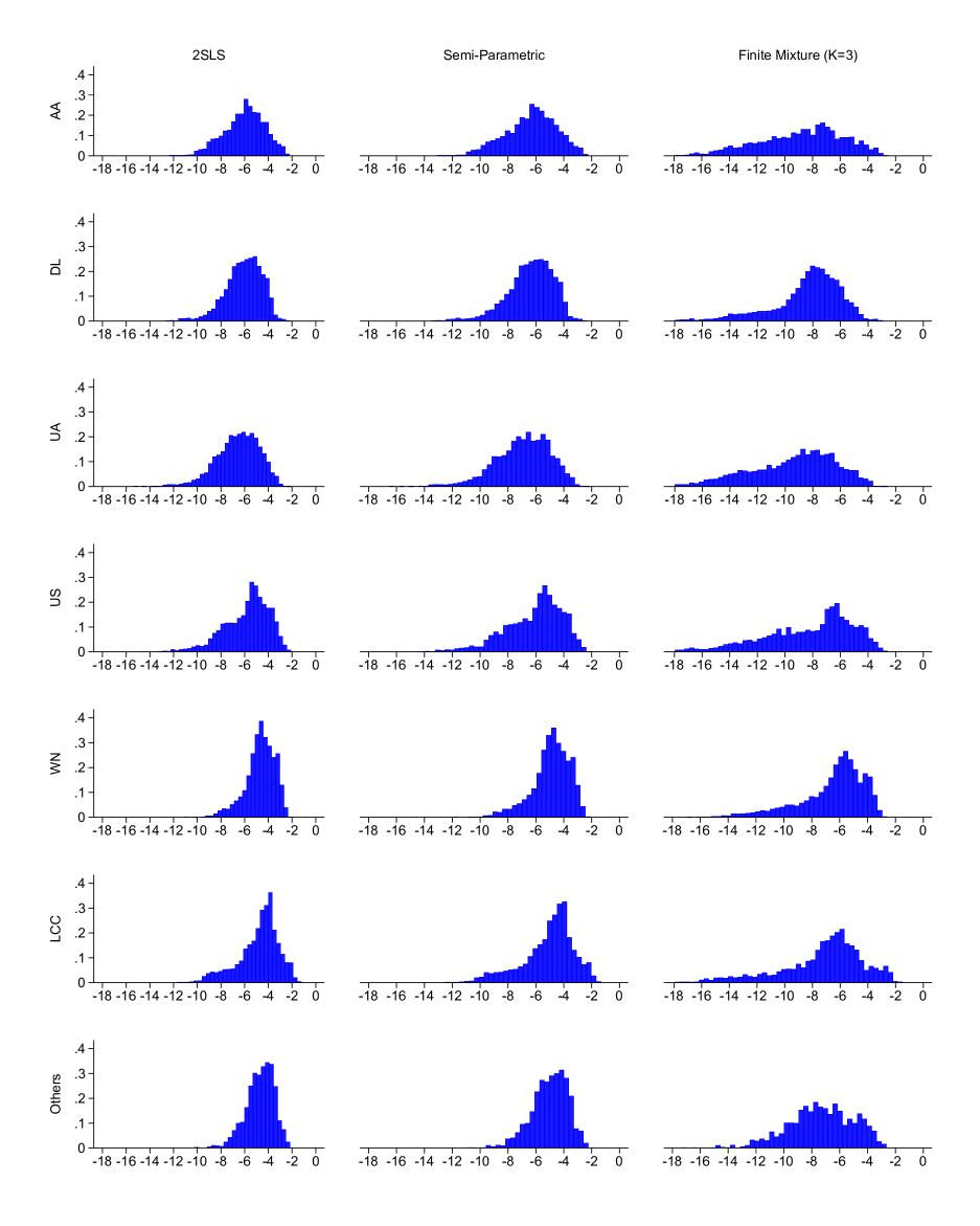
Figure 1: Empirical Distribution of Estimated Elasticities (Airline-Market-Quarter level)

The histograms depicted in the first two columns are very similar. In contrast, the histograms based on the finite mixture estimates showcase significant alterations in both the location and the dispersion of the distribution of elasticities. Across all airlines, the incorporation of larger estimates for $\widehat{\alpha}$ and $\widehat{\sigma}$ using the mixture method leads to a noticeable leftward shift and an amplification in the spread of the histograms. These changes in the distributions’ location and dispersion have important economic implications.

6.4 Estimation of costs and counterfactual experiments

In this paper, we focus on the consistent estimation of demand parameters in the presence of endogenous product entry. However, relying on the structure of our market equilibrium model, it is straightforward for researchers to estimate marginal costs, entry costs, and the joint distribution of unobservable variables. Armed with these estimated primitives, a wide array of counterfactual experiments can be undertaken. In this subsection, and within the framework of our empirical application, we offer a succinct overview of these supplementary estimation procedures.

6.4.1 Marginal costs

Based on an assumption about the nature of competition, such as Nash-Bertrand competition, we are able to derive marginal cost estimates at the airline-market-quarter level by treating the residuals in the pricing equation as estimates of these costs. It is important to note that these marginal costs can be computed only for those products that we observe being active in the market.

For some empirical questions, the researcher may need to estimate the marginal cost function: that is, the function that represents the causal effect of product characteristics and output on marginal costs. For this purpose, the researcher needs to estimate the parameters of a regression equation wherein the dependent variable is the marginal cost estimate, and exogenous product characteristics $\boldsymbol{x}_{jt}$ and output $q_{jt}$ are the explanatory variables. A crucial consideration is that this regression equation is subject to selection bias due to endogenous product entry. Remarkably, the structure of the selection term in this equation mirrors that used in the estimation of the demand equation. We can then control for selection bias in the estimation of the marginal cost function using exactly the same control variables that we have used for the estimation of the demand parameters.

6.4.2 Demand and marginal cost unobservables

The consistent estimation of demand and marginal cost parameters inherently yields consistent estimates for the corresponding unobservable variables: $\xi_{jmt}$ and $\omega_{jmt}$. These unobservables are estimated as residuals within the estimated equations. While the estimation of these equations is subject to selection bias, the introduction of controls for selection enables us to achieve consistent estimation of the structural parameters and of the variables $\xi_{jmt}$ and $\omega_{jmt}$ for the products observed being active in the market.

Naturally, the more complex estimation of the probability distribution or stochastic process governing these unobservables for all products, both those observed being active and inactive in the market, requires one to address the issue of endogenous selection.

6.4.3 Counterfactuals at the intensive margin

Given estimates of demand and marginal cost parameters, researchers can perform counterfactual experiments involving changes to exogenous characteristics of demand and marginal costs but keeping the market structure and, more specifically, the set of active products, as constant. Such counterfactual scenarios are often encountered within applications of the widely employed BLP framework.

Importantly, once the challenge of endogenous selection has been addressed in the estimation of demand and marginal cost parameters, counterfactual experiments that uphold constant the set of products and market structure can be performed without further complications.

6.4.4 Counterfactuals at the extensive margin

Another class of counterfactual experiments involves changes to the ensemble of active firms and/or products within the market. In this category, the most straightforward experiment entails the exogenous removal of certain products from the market. Given the availability of data on the exogenous demand and marginal cost attributes of all products, performing this type of experiment does not significantly differ from the counterfactuals at the intensive margin previously discussed. This type of counterfactual includes as a particular case the evaluation of a counterfactual merger which ignores firms’ endogenous responses at the extensive margin.

Counterfactual experiments that involve the introduction of new products necessitate data on the exogenous attributes of the new or hypothetical products. In our empirical analysis of the airline industry, we observe $\boldsymbol{x}_{jmt}$ for every airline-market-quarter product, irrespective of whether the product is active in the market. Specifically, data on the airline’s hub size at both the origin and destination airports, as well as the airline-quarter fixed effects, are available for both existing products and potential entrants. However, the unobservable factors $\xi_{jmt}$ and $\omega_{jmt}$ are unknown to the researcher for potential entrants. To perform this type of counterfactual, the researcher needs to determine the values of these unobservables also for the potential entrants.

In principle, the researcher could set values for $\xi_{jmt}$ and $\omega_{jmt}$ for the new products at the unconditional mean of these variables, which is zero. However, this approach raises a significant concern: it contradicts the underlying reality that the airline opted not to enter in this particular market. To establish values of $\xi_{jmt}$ and $\omega_{jmt}$ that align with observed endogenous entry decisions, one must consider $\mathbb{E}\left(\xi_{jmt}|\boldsymbol{x}_{mt},a_{jmt}=0\right)$ and $\mathbb{E}\left(\omega_{jmt}|\boldsymbol{x}_{mt},a_{jmt}=0\right)$ respectively.

While our estimation method yields consistent semiparametric estimates for the expected values $\mathbb{E}(\xi_{jmt}|\boldsymbol{x}_{mt},a_{jmt}=1)$ and $\mathbb{E}(\omega_{jmt}|\boldsymbol{x}_{mt},a_{jmt}=1)$, it is silent with respect to $\mathbb{E}(\xi_{jmt}|\boldsymbol{x}_{mt},a_{jmt}=0)$ and $\mathbb{E}(\omega_{jmt}|\boldsymbol{x}_{mt},a_{jmt}=0)$. Achieving point identification for the latter requires supplementary constraints, such as parametric assumptions or symmetry restrictions. An alternative approach instead involves estimating semiparametric bounds for these expected values. This information can then be harnessed to select appropriate values for $\xi_{jmt}$ and $\omega_{jmt}$.

7 Conclusions

In local geographic markets, we typically find only a subset of all the differentiated products available in an industry. Firms strategically select specific products that better match the preferences of local consumers. When making market entry decisions, firms possess information about the demand for their products, particularly regarding unobservable demand components. Firms tend to enter markets with higher expected demand. Neglecting this selection process can introduce significant biases in the estimation of demand parameters. This issue is common across various demand applications and industries. Existing methods to address this issue typically rely on strong parametric assumptions about demand unobservables and firms’ information.

In this paper, we investigate the identification of demand parameters within a structural model that encompasses demand, price competition, and market entry (static or dynamic), while specifying the distribution of demand unobservables in a nonparametric finite mixture manner. The paper makes three main contributions. First, it establishes sequential identification of the demand parameters in this model. We demonstrate that the selection term in the demand equation results from a convolution of the probabilities of product entry for each discrete unobserved market type and the densities associated with these market types. We show that data on firms’ product entry decisions nonparametrically identify the probabilities of product entry conditional on the market type and the density of unobserved market types. Under mild conditions on the observable variables, demand parameters are identified after controlling for the nonparametric entry probabilities and densities for each market type.

Second, we propose a simple two-step estimator to address endogenous selection. In the first step, we estimate a nonparametric finite mixture model to determine the choice probabilities of product entry. In the second step, demand parameters are estimated using a Generalized Method of Moments (GMM) approach that accounts for both endogenous product availability and price endogeneity.

Third, we illustrate the proposed method by applying it to data from the airline industry. The findings highlight the importance of allowing for a finite mixture of unobserved market types when controlling for endogenous product entry, as failure to do so can lead to significant biases.

References

- (1)
- Abaluck and Adams-Prassl (2021) Abaluck, J., and A. Adams-Prassl (2021): “What do consumers consider before they choose? Identification from asymmetric demand responses,” The Quarterly Journal of Economics, 136(3), 1611–1663.
- Aguirregabiria, Collard-Wexler, and Ryan (2021) Aguirregabiria, V., A. Collard-Wexler, and S. Ryan (2021): “Dynamic games in empirical industrial organization,” in Handbook of Industrial Organization, Volume 4, ed. by K. Ho, A. Hortaçsu, and A. Lizzeri, pp. 225–343. Elsevier.
- Aguirregabiria and Ho (2012) Aguirregabiria, V., and C.-Y. Ho (2012): “A dynamic oligopoly game of the US airline industry: Estimation and policy experiments,” Journal of Econometrics, 168(1), 156–173.
- Aguirregabiria and Mira (2007) Aguirregabiria, V., and P. Mira (2007): “Sequential estimation of dynamic discrete games,” Econometrica, 75(1), 1–53.
- Aguirregabiria and Mira (2019) (2019): “Identification of games of incomplete information with multiple equilibria and unobserved heterogeneity,” Quantitative Economics, 10(4), 1659–1701.
- Ahn and Powell (1993) Ahn, H., and J. Powell (1993): “Semiparametric estimation of censored selection models with a nonparametric selection mechanism,” Journal of Econometrics, 58(1-2), 3–29.