Topological Augmentation for
Class-Imbalanced Node Classification

Abstract

Class imbalance is prevalent in real-world node classification tasks and often biases graph learning models toward majority classes. Most existing studies root from a node-centric perspective and aim to address the class imbalance in training data by node/class-wise reweighting or resampling. In this paper, we approach the source of the class-imbalance bias from an under-explored topology-centric perspective. Our investigation reveals that beyond the inherently skewed training class distribution, the graph topology also plays an important role in the formation of predictive bias: we identify two fundamental challenges, namely ambivalent and distant message-passing, that can exacerbate the bias by aggravating majority-class over-generalization and minority-class misclassification. In light of these findings, we devise a lightweight topological augmentation method ToBA to dynamically rectify the nodes influenced by ambivalent/distant message-passing during graph learning, so as to mitigate the class-imbalance bias. We highlight that ToBA is a model-agnostic, efficient, and versatile solution that can be seamlessly combined with and further boost other imbalance-handling techniques. Systematic experiments validate the superior performance of ToBA in both promoting imbalanced node classification and mitigating the prediction bias between different classes.

1 Introduction

Node classification is one of the most fundamental tasks in graph learning with many important real-world applications such as fraud detection [2], social network analysis [44], and cybersecurity [41]. Graph Neural Networks (GNNs) have shown remarkable success in various graph mining tasks based on their powerful representation learning capability. However, real-world graphs are often inherently class-imbalanced, i.e., the sizes of unique classes vary significantly, and a few majority classes have overwhelming numbers in the training set. In such cases, GNNs are prone to be biased toward the majority classes and thus perform poorly on minority classes [7, 34, 39, 54].

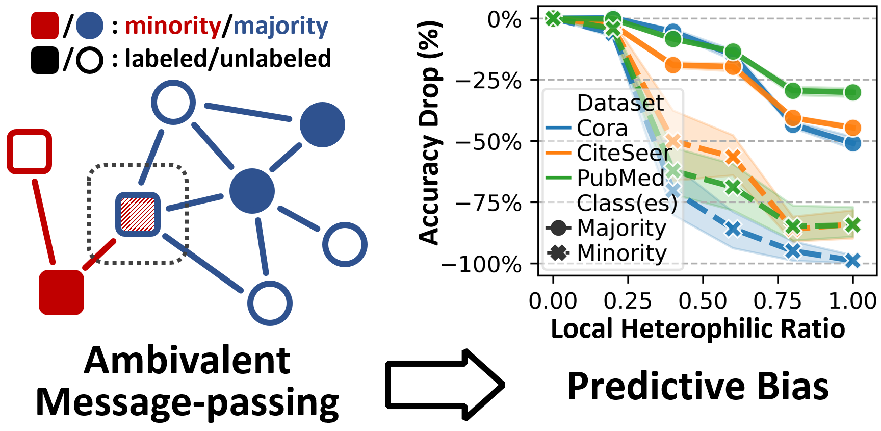
(a) Impact of ambivalent message-passing on the predictive bias in IGL. The performance discrepancy (bias) between minority and majority classes enlarges as the proportion of heterophilic neighbors increases.

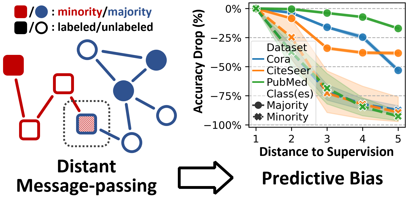
(b) Impact of distant message-passing on the predictive bias in IGL. The performance discrepancy (bias) between minority and majority classes enlarges as the distance to the nearest same-class labeled node increases.

Figure 1: How ambivalent and distant message-passing exacerbate the predictive bias in IGL tasks. Empirical results are derived from benchmark IGL datasets [37] employed in recent studies [7, 34, 40].

While the class imbalance in graph data can be mitigated by adopting generic imbalanced learning techniques, e.g., class-wise reweighting and resampling [6, 9], the improvement can be limited due to the neglection of the topological structure of graph data. Recent studies propose more sophisticated strategies for Imbalanced Graph Learning (IGL), such as reweighing training nodes based on their structural roles in the graph [7], extending the classic SMOTE [6] oversampling algorithm to graph data [54], and synthesizing ego networks to overcome the neighbor-memorization problem for minority classes [34]. These solutions are mainly node-centric and aim to balance the training data by node-level manipulations like reweighting [7] and resampling [54, 34]. Although some studies have utilized topology information to guide node synthesis or weight computing, the role of graph topology in shaping model prediction bias in IGL has been seldom discussed in the literature. This prompts us to approach the IGL problem from a topology-centric perspective, which allows us to shed new light on IGL from several unexplored but intriguing aspects. Specifically, we conduct in-depth investigations to explore: (i) the influence of graph topology on predictive bias in IGL, (ii) the impact of the message-passing on the learning of distinct classes, and (iii) the potential of topological manipulation in mitigating the class imbalance bias and enhancing existing IGL techniques.

Our findings reveal that the inherent class imbalance is not the sole source of predictive bias: undesired factors concealed in graph topology can also disrupt the message-passing-based learning process and introduce a substantial level of bias. Specifically, we identify two fundamental topological challenges that exacerbate the class-imbalance bias: (i) Ambivalent message-passing (AMP) refers to the high ratio of local heterophilic connections that cause message-passing to introduce incorrect learning signals to a node. This issue can amplify the influence of class imbalance, as the majority classes with more training nodes can over-generalize through such connections and cause more misclassifications in minority classes, as depicted in Fig. 1(a). (ii) Distant message-passing (DMP) corresponds to the poor connectivity to labeled nodes that makes message-passing fail to deliver correct learning signals. This issue can worsen misclassification in minority classes, which are poorly represented in the feature space and thus rely heavily on message-passing for representation learning, as shown in Fig. 1(b). The preceding analysis demonstrates how local topological patterns of nodes introduce a class-related bias in their learning process. We note that while the literature has explored related topics on graph (global) heterophily [3, 8] and long-distance propagation [11], they are deemed orthogonal issues to IGL and their impact under class imbalance is seldom discussed.

Armed with these analyses, we propose ToBA (Topological Balanced Augmentation), a novel, fast, and model-agnostic framework to handle the topological challenges in class-imbalanced node classification. At the core of ToBA are the following: (i) node risk estimation to measure the risk of being influenced by AMP and DMP for each node; (ii) candidate class selection to identify potential ground-truth (candidate) classes for high-risk nodes that are prone to misclassification; (iii) topology augmentation to connect high-risk nodes to their candidate class prototype by dynamically synthesizing virtual super-nodes and edges, thereby rectifying their learning with augmented topological information. We highlight that the nimble design of ToBA makes it model-agnostic and computationally efficient. More importantly, ToBA is orthogonal to most of the existing IGL techniques (e.g., [18, 6, 7, 54, 34]), thus can work hand-in-hand with them and further boost their performance. Extensive experiments on real-world IGL tasks show that ToBA delivers consistent and significant performance boost to various IGL baselines with diverse GNN architectures.

To sum up, our contribution is 3-fold: (i) Problem Definition. We propose to address the source of the class-imbalance bias from an under-explored topology-centric perspective, which may shed new light on IGL research. To our best knowledge, we present the first study on the role of graph topology in the formation of model predictive bias, showing how ambivalent/distant message-passing exacerbates class-imbalance bias in IGL. (ii) Methodology. We propose a lightweight augmentation technique ToBA to handle the topological challenges in class-imbalanced node classification. It is a model-agnostic, efficient, and versatile solution that can be seamlessly combined with and further boost other IGL techniques. (iii) Empirical Results. Systematic experiments and analysis on real-world IGL tasks show that ToBA consistently enhances various IGL techniques with diverse GNN architectures, leading to superior performance in both promoting classification and mitigating the predictive bias. ToBA shows even more prominent advantages in highly-imbalanced IGL tasks.

2 Preliminary

Notations. In this paper, we use bold uppercase letters for matrices (e.g., $\mathbf{A}$), bold lowercase letters for vectors (e.g., $\mathbf{y}$), calligraphic letters for sets (e.g., $\mathcal{V}$), and lowercase letters for scalars (e.g., $d$). Given a $d$-dimensional feature space $\mathcal{X}:\mathbb{R}^{d}$ and an $m$-dimensional label space $\mathcal{Y}:\{c_{0},c_{1},\cdots,c_{m}\}$, a node $v:(\mathbf{x},y)$ is defined in terms of the node feature vector $\mathbf{x}\in\mathcal{X}$ and the node label $y\in\mathcal{Y}$. An edge $e:(u,v)$ exists if nodes $u$ and $v$ are connected. A graph with node set $\mathcal{V}$ and edge set $\mathcal{E}$ is represented as $\mathcal{G}:\{\mathbf{A},\mathbf{X}\}$ with the adjacency matrix $\mathbf{A}\in\mathbb{R}^{|\mathcal{V}|\times|\mathcal{V}|}$ and the node feature matrix $\mathbf{X}\in\mathbb{R}^{|\mathcal{V}|\times d}$. The groundtruth node label vector is denoted as $\mathbf{y}\in\mathbb{R}^{|\mathcal{V}|}$. For simplicity, we use $\mathbf{x}_{i}\in\mathcal{X}$ and $y_{i}\in\mathcal{Y}$ to denote the feature vector and the label of the $i$-th node $v_{i}\in\mathcal{V}$ respectively.

Node classification with GNN. Following recent studies [7, 34, 40, 54], we focus on the class imbalance in transductive semi-supervised node classification . Formally, given a graph $\mathcal{G}=\{\mathbf{A},\mathbf{X}\}$, a labeled node set $\mathcal{V}^{L}$, and a node classifier, e.g., GNN, $F(\cdot;\mathbf{\Theta})$ with parameters $\mathbf{\Theta}$, the goal of node classification is to optimize the classifier $F(\cdot;\mathbf{\Theta})$ such that the generated prediction vector $\hat{\mathbf{y}}$ approximates the groundtruth label vector $\mathbf{y}$. A typical GNN derives node representations by recursively passing and aggregating the node features through multiple message-passing-based convolution layers. The $l$-th GNN layer updates node feature $\mathbf{x}^{(l+1)}_{v}$ from $\mathbf{x}^{(l)}_{v}$ by: $x^{(l+1)}_{v}=\gamma_{l}\left(x^{(l)}_{v},\psi_{l}\left(\{m_{l}(x^{(l)}_{v},x^{(l)}_{u},w_{v,u})|u\in\mathcal{N}(v)\}\right)\right),$ where $m_{l}$ is the message-passing function, $\psi_{l}$ is aggregation operator, $\gamma_{l}$ is feature update function, and $w_{u,v}$ is the weight of edge $(u,v)$.

Class-imbalanced node classification. A standard node classifier is usually biased under imbalance since classes with abundant training samples contribute most of the loss and gradients [4, 19]. They dominate the training and lead to biased predictive performance [24]. In this case, we refer to the classes with abundant/absent training data as majority/minority classes. Without loss of generality, we denote minority classes as positive classes ($\mathcal{Y}^{+}$) and majority classes as negative ones ($\mathcal{Y}^{-}$). For class-imbalanced node classification, we have: $|\{y=c_{i}|(\mathbf{x},y)\in\mathcal{V}^{L}\}|\ll|\{y=c_{j}|(\mathbf{x},y)\in\mathcal{V}^{L}\}|,\forall c_{i}\in\mathcal{Y}^{+},c_{j}\in\mathcal{Y}^{-}.$ Such imbalanced training data makes it harder for GNN to learn the pattern of minority classes due to the lack of training signals, and therefore, makes GNN more prone to be biased towards majority classes $\mathcal{Y}^{-}$ and perform poorly on minority classes $\mathcal{Y}^{+}$. The goal of class-imbalanced node classification is to learn a balanced classifier $F(\cdot;\mathbf{\Theta})$ from imbalanced supervision $\mathcal{V}^{L}$ in order to perform well on both majority classes $\mathcal{Y}^{-}$ and minority classes $\mathcal{Y}^{+}$.

Definition 1

Class-imbalanced Node Classification. Given a graph $\mathcal{G}:\{\mathbf{A},\mathbf{X}\}$ with labeled set $\mathcal{V}^{L}$ where $|\{y=c_{i}|(\mathbf{x},y)\in\mathcal{V}^{L}\}|\ll|\{y=c_{j}|(\mathbf{x},y)\in\mathcal{V}^{L}\}|,$ $\forall c_{i}\in\mathcal{Y}^{+}$ (minority classes), $c_{j}\in\mathcal{Y}^{-}$ (majority classes). We aim to learn a node classifier $F(\cdot;\mathbf{\Theta})$ that works well for both $\mathcal{Y}^{-}$ and $\mathcal{Y}^{+}$:

$$F(\mathbf{A},\mathbf{X};\mathbf{\Theta})\to\mathbf{y}$$

3 Handling Class-imbalance via Topological Augmentation

As discussed in Section 1, factors in graph topology, i.e., ambivalent message-passing (AMP) and distant message-passing (DMP), also play important roles in the formation of predictive bias in IGL. In order to handle the negative effect of AMP and DMP, we propose a lightweight framework ToBA (Topological Balanced Augmentation) to mitigate the bias and boost classification in IGL. Specifically, ToBA is a graph data augmentation technique that can be integrated into any GNN training procedure to perform dynamic and adaptive topological augmentation in each learning step.

ToBA has three core components: (§ 3.1) node risk estimation: for each node, we first determine its risk of being influenced by AMP and DMP w.r.t. $F(\cdot;\mathbf{\Theta})$; (§ 3.2) candidate class selection: for high-risk nodes that are prone to misclassification, we independently select candidate classes for rectifying learning based on estimated node-class similarity. (§ 3.3) virtual topology augmentation: finally, we dynamically synthesize virtual super-nodes and edges to rectify graph learning with augmented topological information. An overview of the proposed ToBA framework is shown in Fig. 2. We now elaborate on technical details with related discussions for each component.

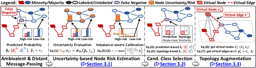
Figure 2: The proposed ToBA framework, best viewed in color.

3.1 Node Risk Estimation

The first step in mitigating predictive bias caused by AMP and DMP is to locate the nodes that are affected by them. Previous studies have shown that heterophilic/poor connectivity to supervision can disturb GNN learning and the associated graph-denoising process for affected nodes [33, 49, 30], and further, yield high uncertainty in the predictive model [43, 55]. This motivates us to utilize the model prediction uncertainty to estimate nodes’ risk of being misclassified due to AMP/DMP.

Uncertainty-based risk estimation. While there exist various techniques (e.g., Bayesian-based [52, 13], Jackknife sampling [21] and more [27, 55]) for evaluating uncertainty in node classification, they often necessitate modifying the model architecture, and the associated computational costs are typically non-negligible. To achieve fast and model-agnostic topological augmentation, we adopt a simple but effective approach to compute node uncertainty of model $F(\cdot;\mathbf{\Theta})$ based on the predicted probabilities. Formally, for a node $v_{i}$, consider model $F(\cdot;\mathbf{\Theta})$’s predicted probabilities $\hat{\mathbf{p}}_{i}:[\hat{p}_{i}^{(1)},\hat{p}_{i}^{(2)},\cdots,\hat{p}_{i}^{(m)}]$, where $\hat{p}_{i}^{(j)}=P(y_{i}=c_{j}|\mathbf{A},\mathbf{X},\mathbf{\Theta})$ is the estimated probability of node $v_{i}$ belonging to class $c_{j}$. By taking the $\operatorname*{arg\,max}$ operator over $\hat{\mathbf{p}}_{i}$, we obtain the corresponding one-hot indicator vector $\mathds{1}_{\hat{y}_{i}}\in\{0,1\}^{m}$ with $\mathds{1}_{\hat{y}_{i}}^{(\hat{i})}=1$, where $\hat{i}=\operatorname*{arg\,max}_{j}\hat{p}_{i}^{(j)}$, and $\hat{y}_{i}=c_{\hat{i}}$ is the predicted label. We measure the node uncertainty score $\mathbb{U}_{\mathbf{\Theta}}(v_{i})$ w.r.t. model $F(\cdot;\mathbf{\Theta})$ by the total variation $d_{\text{TV}}$ between the predicted probabilities $\hat{\mathbf{p}}_{i}$ and the corresponding indicator vector $\mathds{1}_{\hat{y}_{i}}$:

$$\mathbb{U}_{\mathbf{\Theta}}(v_{i})=d_{\text{TV}}(\hat{\mathbf{p}}_{i},\mathds{1}_{\hat{y}_{i}})=\frac{1}{2}\sum\limits_{j=1}^{m}|\hat{\mathbf{p}}_{i}^{(j)}-\mathds{1}_{\hat{y}_{i}}^{(j)}|.$$ (1)

Intuitively, a node has higher uncertainty if the model is less confident about its current prediction, i.e., with a smaller $\hat{p}_{i}^{(\hat{i})}$. We note that this metric can be naturally replaced by other uncertainty measures, here we use $d_{\text{TV}}$ for its simplicity and $\mathcal{O}(1)$ time complexity when computed in parallel on GPU.

Calibrating the absolute uncertainty. The node uncertainty score in Eq. (1) needs to be further calibrated for different classes in IGL. For one, nodes of minority classes usually exhibit higher overall uncertainty scores compared to those in majority classes due to the lack of training instances. For another, AMP and DMP can further exacerbate the influence of imbalance and cause majority-class over-generalization and minority-class misclassification. This leads to a higher prediction error, and furthermore, higher variance in the uncertainty scores for minority classes compared with the majority ones. For the above reasons, direct usage of node uncertainty as the risk score will cause minority-class nodes to be treated as high-risk nodes, which is contrary to our intention of correcting the false negative (i.e., minority nodes that are wrongly predicted as majority class) predictions in order to mitigate class imbalance.

To cope with the high mean and variance of minority-class uncertainty, we propose imbalance-aware relative normalization to calibrate the absolute uncertainty score. Formally, for node $v_{i}$ with uncertainty score $\mathbb{U}_{\mathbf{\Theta}}(v_{i})$ and predicted label $\hat{y}_{i}$, its calibrated uncertainty score can be computed as:

$$\mathbb{U}^{*}_{\mathbf{\Theta}}(v_{i})=\frac{\mathbb{U}_{\mathbf{\Theta}}(v_{i})-\mu_{\hat{y}_{i}}}{\omega_{\hat{y}_{i}}},\text{ where }\mu_{\hat{y}_{i}}=\sum_{v_{j}\in\hat{\mathcal{V}}_{\hat{y}_{i}}}\mathbb{U}_{\mathbf{\Theta}}(v_{j})/|\hat{\mathcal{V}}_{\hat{y}_{i}}|\text{ and }\omega_{\hat{y}_{i}}=|\mathcal{V}^{L}_{\text{max}}|/|\mathcal{V}^{L}_{\hat{y}_{i}}|.$$ (2)

In Eq. (2), $\mu_{\hat{y}_{i}}$ with $\hat{\mathcal{V}}_{\hat{y}_{i}}=\{v_{j}|\hat{y}_{j}=\hat{y}_{i},v_{j}\in\mathcal{V}\}$ is the average uncertainty score of all nodes with predicted label $\hat{y}_{i}$. $\omega_{\hat{y}_{i}}$ with $|\mathcal{V}^{L}_{\hat{y}_{i}}|=|\{v_{j}|y_{j}=\hat{y}_{i},v_{j}\in\mathcal{V}^{L}\}|$ and $|\mathcal{V}^{L}_{\text{max}}|=\max_{c_{j}\in\mathcal{Y}}|\mathcal{V}^{L}_{c_{j}}|$ is the normalization weight determined by the relative size of the predicted class $\hat{y}_{i}$ in the training set. Specifically, minority classes with smaller $|\mathcal{V}^{L}_{\hat{y}_{i}}|$ will have larger normalization weights $\omega_{\hat{y}_{i}}$. Intuitively, Eq. (2) first compute $v_{i}$’s class-aware relative uncertainty by subtracting the class average $\mu_{\hat{y}_{i}}$, and then scale down its uncertainty by the imbalance-aware normalization weight $\omega_{\hat{y}_{i}}$, i.e., minority classes will have smaller risks. Finally, we derive the risk score $r_{i}$ by only keeping the positive scores since we only care about the high-risk nodes with above-class-average uncertainty:

$$r_{i}=\text{max}(\mathbb{U}^{*}_{\mathbf{\Theta}}(v_{i}),0).$$ (3)

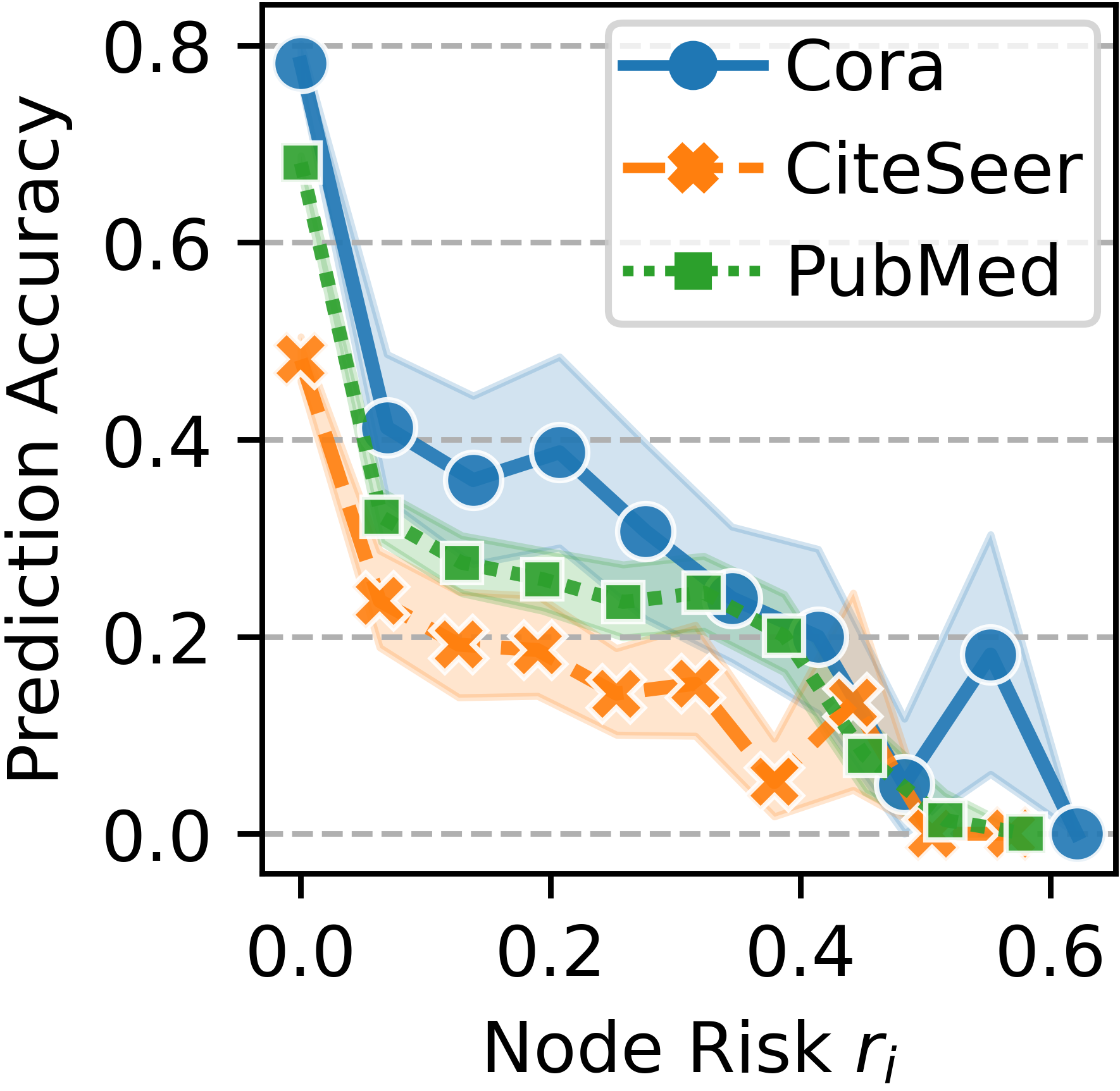
Figure 3: The negative correlation between the estimated node risk (x-axis) and the prediction accuracy (y-axis) in real-world IGL tasks. We apply 10 sliding windows to compute the mean and deviation of the accuracy.

Empirical justification. We validate the effectiveness of the proposed node risk assessment method, as shown in Fig. 3. The results indicate that our approach while being computationally efficient, can also accurately estimate node misclassification risk across various real-world IGL tasks.

3.2 Candidate Class Selection

With the estimated risk scores of being affected by AMP/DMP, we can locate high-risk nodes that are prone to misclassification (e.g., false negatives). Ground truth labels of such nodes are likely from their candidate classes (i.e., non-predicted classes $\in\{c_{j}|c_{j}\neq\hat{y}_{i}\}$). In this section, we discuss how to support high-risk nodes’ learning by leveraging additional topological information from other candidate classes. Since augmenting with signals uniformly/randomly drawn from all candidate classes can only introduce noise to the learning, we need to identify the source candidate class for all high-risk node, i.e., given the model $F(\cdot;\mathbf{\Theta})$, for each high-risk node $v_{i}$ we need to estimate the likelihood that $v_{i}$ comes from each candidate class $P(y_{i}=c_{j};\mathbf{A},\mathbf{X},\mathbf{\Theta}),\forall c_{j}\neq\hat{y}_{i}$. In this paper, we approach the problem by estimating the similarity of nodes to candidate classes. Again, with efficiency as our top priority, we consider two efficient methods with $\mathcal{O}(1)$/$\mathcal{O}(n)$ time complexity in practice: prediction-based and topology-based similarity estimation.

Prediction-based similarity estimation. The first natural approach to estimate $P(y_{i}=c_{j};\mathbf{A},\mathbf{X},\mathbf{\Theta})$ is to utilize the model’s predicted probabilities. Formally, let us denote the similarity vector of node $v_{i}$ as $\hat{\mathbf{s}}_{i}=[\hat{s}_{i}^{(1)},\hat{s}_{i}^{(2)},...,\hat{s}_{i}^{(m)}]$ with $\hat{s}_{i}^{(j)}\in[0,1]$ be $v_{i}$’s similarity to class $c_{j}$ and let $\sum_{j=1}^{m}\hat{s}_{i}^{(j)}=1$ (i.e., $\hat{\mathbf{s}}_{i}$ is normalized). Then for prediction-based similarity estimation, we have:

$$\hat{\mathbf{s}}_{i}=[\hat{s}_{i}^{(1)},\hat{s}_{i}^{(2)},...,\hat{s}_{i}^{(m)}],\hat{s}_{i}^{(j)}=\left\{\begin{aligned} &\hat{p}_{i}^{(j)}/Z&,\ &c_{j}\neq\hat{y}_{i}\\ &0&,\ &c_{j}=\hat{y}_{i}\\ \end{aligned}\right.,$$ (4)

where $Z=1-\hat{p}_{i}^{\hat{y}_{i}}$ is the normalization term. Importantly, we exclude $p_{\hat{y}_{i}}$ in the similarity computation since for a high-risk node, its current prediction for $\hat{y}_{i}$ is likely to be influenced by AMP and/or DMP, and we want to rectify its learning by considering the model’s output for other candidate classes. After this, Eq. (4) assigns similarities to candidate classes according to the predicted probabilities, i.e., higher the probability that $F(\cdot;\mathbf{\Theta})$ predicts that node $v_{i}$ belongs to class $c_{j}$, higher the similarity between $v_{i}$ and $c_{j}$. This can be done in matrix form on GPU with $\mathcal{O}(1)$ time complexity.

Topology-based similarity estimation. Beyond the above method, we further explore local topology structure for similarity estimation. Since we consider homophily graph [1, 31] where neighboring nodes share similar labels, we use the pseudo neighbor label distribution of high-risk nodes to measure their similarities to candidate classes. Formally, let $\mathcal{N}(v)$ be the neighbor node set of $v$, we have:

$$\hat{\mathbf{s}}_{i}=[\hat{s}_{i}^{(1)},\hat{s}_{i}^{(2)},...,\hat{s}_{i}^{(m)}],\hat{s}_{i}^{(j)}=\left\{\begin{aligned} &|\{v_{k}|\hat{y}_{k}=c_{j},v_{k}\in\mathcal{N}(v_{i})\}|/Z&,\ &c_{j}\neq\hat{y}_{i}\\ &0&,\ &c_{j}=\hat{y}_{i}\\ \end{aligned}\right.,$$ (5)

where $Z=|\mathcal{N}(v_{i})|-|\{v_{k}|\hat{y}_{k}=\hat{y}_{i},v_{k}\in\mathcal{N}(v_{i})\}|$ is the normalization term. Intuitively, the similarity score between a high-risk node $v_{i}$ and a candidate class $c_{j}$ is proportional to the label frequency of $c_{j}$ among the adjacent nodes $\mathcal{N}(v_{i})$. Different from the prediction-based similarity, topology-based method relies both on node-level predictions and the local topology patterns. The above computation can also be done in matrix form with $\mathcal{O}(n)$ complexity. Detailed complexity analysis can be found in Section 4. Fig. 2 provides an illustrative example of the two estimations.

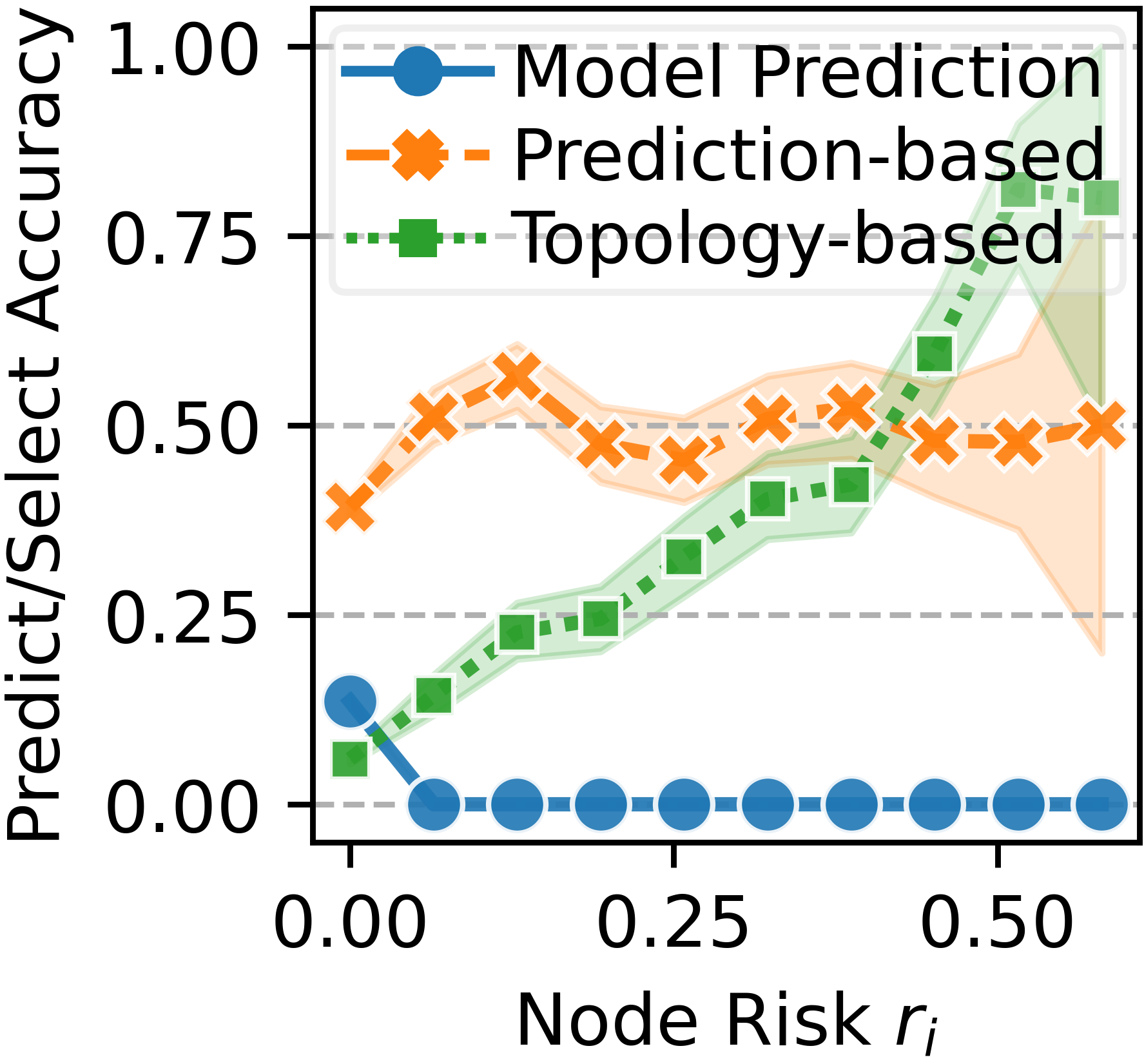
Figure 4: Minority-class accuracy of model prediction, i.e., $\hat{y}_{i}$, and max-similarity-based candidate selection i.e., $\hat{y}^{s}_{i}=c_{\text{argmax}(\mathbf{s}_{i})}$, on PubMed dataset. We show the accuracy (y-axis) w.r.t. the risk (x-axis) with 10 sliding windows.

Empirical justification. A comparison between the two strategies is given in Fig. 4. We can see that almost all minority nodes with positive risk ($r_{i}>0$) are misclassified, but both strategies can effectively find alternatives with significantly higher chances to be the ground truth class for high-risk nodes. However, we note that this result does not fully reflect the pros and cons of different similarity estimation methods since we only consider the best candidates with the highest similarity score. In practice, the whole similarity vector is used for topological augmentation.

3.3 Virtual Topology Augmentation

Having the derived node risk and similarities scores, now we discuss how to utilize them to perform topological augmentation. The general idea is to connect high-risk nodes to their candidate classes so as to integrate information from nodes that share similar patterns (mitigate AMP), even if they are not closely adjacent to each other in the graph topology (mitigate DMP), thus achieving less-biased IGL.

Why virtual super-nodes and edges? A natural way to connect a high-risk node and its candidate classes is to add edges between it and nodes from candidate classes in the original graph. However, this can be problematic in practice as a massive number of possible edges could be generated and greatly disturb the original topology structure. To achieve augmentation without disrupting the graph topology, we aim to create virtual “short-cuts” that pass aggregated candidate class information to high-risk nodes. This is achieved by injecting a few virtual super-nodes (one for each class) and connecting them to high-risk nodes according to the risk and similarity scores. By doing so, we create implicit shortcuts between the target high-risk node and nodes that exhibit similar patterns, even if they are not closely adjacent in the original graph, thus mitigating both AMP and DMP.

Virtual topology generation. Equipped with the above analysis, we build one virtual prototype super-node for each class by feature mean aggregation to represent its general pattern in the feature space. For class $c_{j}$, we build its virtual super-node $v^{*}_{j}:(\mathbf{x}^{*}_{j},y^{*}_{j})$ with pseudo-label $y^{*}_{j}=c_{j}$, and we compute its features $\mathbf{x}^{*}_{j}$ by averaging all nodes that are predicted to be from class $c_{j}$:

$$\mathbf{x}^{*}_{j}=\sum_{v_{i}\in\hat{\mathcal{V}}_{c_{j}}}\frac{\mathbf{x}_{i}}{|\hat{\mathcal{V}}_{c_{j}}|},\text{where }\hat{\mathcal{V}}_{c_{j}}=\{v_{i}|\hat{y}_{i}=c_{j},v_{i}\in\mathcal{V}\}.$$ (6)

We then add virtual edges based on the risks and similarities. Let us denote the derived virtual super-nodes as $\{v^{*}_{1},v^{*}_{2},...,v^{*}_{m}\}$. Given node $v_{i}$ with prediction risk $r_{i}$ and candidate-class similarity vector $\mathbf{s}_{i}:[s_{i}^{(1)},s_{i}^{(2)},...,s_{i}^{(m)}]$, the corresponding virtual link probability vector can be computed by:

$$\mathbf{p}^{*}_{i}:[p_{i}^{(1)},p_{i}^{(2)},...,p_{i}^{(m)}],\text{where }p_{i}^{(j)}=r_{i}\times s_{i}^{(j)}.$$ (7)

The $j$-th element of $\mathbf{p}^{*}_{i}$ is the probability of connecting node $v_{i}$ to the virtual node $v^{*}_{j}$ of class $c_{j}$. The virtual edges are then independently sampled w.r.t. $\mathbf{p}^{*}_{i}$. Note that $\sum\mathbf{p}_{i}^{*}=r_{i}$ since the similarity vector $\mathbf{s}_{i}$ is normalized. In other words, node risk $r_{i}\in[0,1]$ determines the expected number of virtual links connected to $v_{i}$, and the similarity vector $\mathbf{s}_{i}$ determines how to distribute the probability to each candidate class. We note that this simple and efficient design also enables implicit multi-hop propagation: consider a node $v_{i}$ and virtual super-node $v^{*}_{j}$, the temporary virtual edge $(v_{i},v^{*}_{j})$ enables $v_{i}$ to indirectly receive information from all nodes in $\hat{\mathcal{V}}_{c_{j}}$,

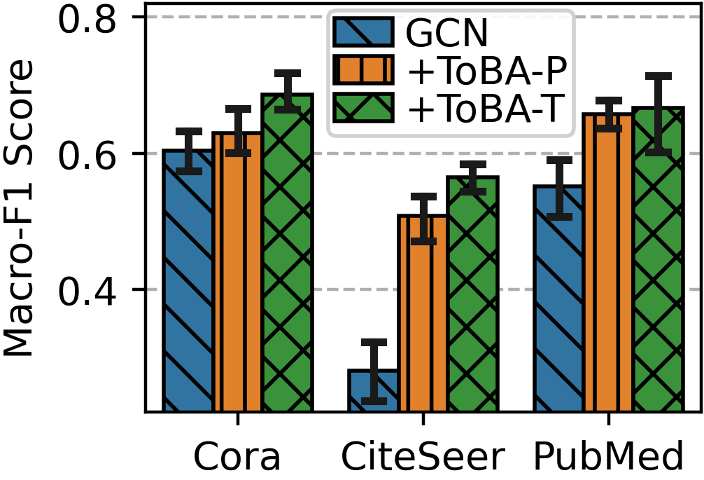
Figure 5: ToBA with prediction-/topology-based candidate class selection (i.e., ToBA_P/T) achieve superior classification performance in various IGL tasks [34].

this further helps to alleviate ambivalent and, especially, distant message-passing. We provide a quick verification of the validity of ToBA in Fig. 5, and have more comprehensive results and discussions in the next section.

Algorithm 1 ToBA : Topological Balanced Augmentation

1:$\mathcal{G}:\{\mathbf{A},\mathbf{X}\}$ with imbalanced labeled set $\mathcal{V}^{L}$;

2:Initialize: node classifier $F(\cdot;\mathbf{\Theta})$;

3:while not converged do

4:     $\hat{\mathbf{P}},\hat{\mathbf{y}}\leftarrow F(\mathbf{A},\mathbf{X};\mathbf{\Theta})$;

5:     $\mathbf{r}\leftarrow\texttt{RiskEst}(\hat{\mathbf{P}}$, $\hat{\mathbf{y}})$; $\triangleright$ Eq.(1)-(3)

6:     $\hat{\mathbf{S}}\leftarrow\texttt{SimilarityEst}(\mathbf{A},\hat{\mathbf{P}},\hat{\mathbf{y}})$; $\triangleright$ Eq.(4)/(5)

7:     for $j=1$ to $m$ do

8:         Get virtual super-node feature $\mathbf{x}^{*}_{j}$; $\triangleright$ Eq.(6)      

9:     $\mathcal{V}^{*}\leftarrow\{(\mathbf{x}^{*}_{j},c_{j})|1\leq j\leq m\}$

10:     $\mathbf{P}^{*}\leftarrow\hat{\mathbf{S}}\odot\mathbf{r}$ $\triangleright$ Eq.(7)

11:     $\mathcal{E}^{*}\leftarrow$ sampling w.r.t. virtual link probabilities $\mathbf{P}^{*}$;

12:     Derive $\mathbf{X}^{*},\mathbf{A}^{*}$ from $\mathcal{V}\cup\mathcal{V}^{*},\mathcal{E}\cup\mathcal{E}^{*}$;

13:     Update $\mathbf{\Theta}$ with augmented graph $\mathcal{G}^{*}:\{\mathbf{A}^{*},\mathbf{X}^{*}\}$;

14:return a balanced classifier $F(\mathbf{A},\mathbf{X};\mathbf{\Theta})$;

So far, we have finished the discussion of the ToBA . Thanks to the fast computation, we may apply the above augmentation in each GNN training iteration with little extra computational cost. The overall framework of ToBA is summarized in Alg. 1. Note that all the node-wise computation can be parallelized in matrix form in practice, so we define them as follows in Alg. 1: $\mathbf{r}$ is the node risk vector with $r_{i}$ being the $i$-th element. The $i$-th row of the predicted probability matrix $\hat{\mathbf{P}}$, node similarity matrix $\hat{\mathbf{S}}$, and virtual link probability matrix $\mathbf{P}^{*}$ are $\hat{\mathbf{p}_{i}}$, $\hat{\mathbf{s}_{i}}$, $\mathbf{p}^{*}_{i}$ respectively. We provide a more detailed complexity analysis of ToBA in the next section.

4 Experiments

In this section, we carry out systematic experiments and analysis to validate the proposed ToBA framework in the following aspects: (i) Effectiveness in both promoting imbalanced node classification and mitigating the prediction bias between different classes. (ii) Versatility in cooperating with and further boosting various IGL techniques and GNN backbones. (iii) Robustness to extreme class imbalance. (iv) Efficiency in real-world applications. We briefly introduce the experimental setup first, and then present the empirical results and analyses. Please refer to the Appendix for more reproducibility details (§ A), as well as extended empirical results and discussions (§ B).

Table 1: Performance of combining ToBA with 6 IGL baselines $\times$ 5 GNN backbones. We include balanced metrics for both predictive performance (Balanced Accuracy, Macro-F1) and bias (Performance Disparity), and report the relative performance gain of ToBA. For each baseline’s three settings (i.e., Base, + ToBA_P, + ToBA_T), we mark the best/second-best results in bold/underlined.

Dataset (IR=10)

Cora

CiteSeer

PubMed

Metric: BAcc.$\uparrow$

Base

+ ToBAP

+ ToBAT

Base

+ ToBAP

+ ToBAT

Base

+ ToBAP

+ ToBAT

GCN

Vanilla

61.56

65.54+6.47%

69.80+13.39%

37.62

52.65+39.96%

55.37+47.18%

64.23

68.62+6.83%

67.57+5.20%

Reweight

67.65

70.97+4.91%

72.14+6.64%

42.49

57.91+36.28%

58.36+37.35%

71.20

74.19+4.19%

73.37+3.04%

ReNode

66.60

71.37+7.16%

71.84+7.88%

42.57

57.47+35.00%

59.28+39.24%

71.52

73.20+2.35%

72.53+1.42%

Resample

59.48

72.51+21.91%

74.24+24.82%

39.15

57.90+47.88%

58.78+50.14%

64.97

72.53+11.64%

72.87+12.16%

SMOTE

58.27

72.16+23.83%

73.89+26.81%

39.27

60.06+52.95%

61.97+57.82%

64.41

73.17+13.61%

73.13+13.55%

GSMOTE

67.99

68.52+0.78%

71.55+5.23%

45.05

57.68+28.03%

57.65+27.96%

73.99

73.09+-1.22%

76.57+3.49%

GENS

70.12

72.22+3.00%

72.58+3.50%

56.01

60.60+8.19%

62.67+11.88%

73.66

76.11+3.32%

76.91+4.41%

2-11[1pt/1pt]

Best

70.12

72.51+3.41%

74.24+5.87%

56.01

60.60+8.19%

62.67+11.88%

73.99

76.11+2.86%

76.91+3.94%

GAT

Best

69.76

72.14+3.42%

73.29+5.07%

51.50

60.95+18.34%

63.49+23.28%

73.13

75.55+3.31%

75.65+3.45%

SAGE

Best

68.84

71.31+3.58%

73.02+6.08%

52.57

64.36+22.42%

66.35+26.20%

71.55

75.89+6.07%

77.38+8.15%

PPNP

Best

73.74

75.02+1.74%

73.78+0.06%

50.88

66.62+30.93%

65.57+28.86%

72.76

73.37+0.85%

74.90+2.95%

GPRGNN

Best

73.38

74.01+0.86%

74.89+2.05%

54.66

64.16+17.39%

63.89+16.89%

73.56

75.69+2.90%

77.49+5.34%

Metric: Macro-F1$\uparrow$

Base

+ ToBAP

+ ToBAT

Base

+ ToBAP

+ ToBAT

Base

+ ToBAP

+ ToBAT

GCN

Best

69.96

71.62+2.37%

72.82+4.08%

54.45

59.89+9.97%

62.46+14.71%

71.28

75.77+6.30%

76.86+7.83%

GAT

Best

69.96

70.87+1.30%

72.31+3.36%

48.34

60.04+24.21%

62.55+29.40%

71.78

75.13+4.66%

74.96+4.42%

SAGE

Best

68.23

70.40+3.17%

71.71+5.10%

51.05

63.87+25.12%

65.91+29.12%

70.06

75.33+7.52%

76.92+9.79%

PPNP

Best

73.67

73.67+0.00%

73.22-0.61%

45.25

66.18+46.27%

65.20+44.10%

70.65

72.55+2.70%

74.61+5.61%

GPRGNN

Best

73.08

72.89-0.25%

73.54+0.64%

50.34

63.59+26.33%

63.12+25.39%

71.45

75.47+5.64%

77.62+8.64%

Metric: Disparity$\downarrow$

Base

+ ToBAP

+ ToBAT

Base

+ ToBAP

+ ToBAT

Base

+ ToBAP

+ ToBAT

GCN

Best

20.04

14.43-28.00%

15.25-23.92%

16.95

13.82-18.44%

13.93-17.81%

11.93

3.35-71.88%

5.15-56.86%

GAT

Best

20.08

15.05-25.05%

17.32-13.76%

25.21

10.68-57.62%

13.24-47.47%

10.29

3.01-70.79%

4.58-55.49%

SAGE

Best

19.81

13.32-32.75%

14.87-24.93%

19.76

13.17-33.34%

12.78-35.33%

11.76

3.35-71.50%

4.09-65.25%

PPNP

Best

18.09

16.87-6.76%

18.46+2.06%

25.95

14.91-42.55%

19.19-26.02%

14.49

8.04-44.49%

3.95-72.74%

GPRGNN

Best

18.84

16.78-10.96%

17.00-9.75%

22.43

14.83-33.86%

15.98-28.75%

14.40

5.99-58.42%

5.30-63.20%

• *ToBA_P/ToBA_T: ToBA with prediction-/topology-based candidate class selection. We report the average score of 5 independent runs to eliminate randomness

Due to space limitations, we omit the error bar and only report the best performance for most settings, full results can be found in the supplementary material.

Datasets. We validate ToBA on five benchmark datasets for semi-supervised node classification: three from the widely-used Plantoid citation graphs [37] (Cora, CiteSeer, PubMed), and two from the Coauthor networks [38] (CS, Physics) with more nodes & edges and high-dimensional features to test ToBA on large graphs, detailed data statistics can be found in Appendix A.1. For citation networks, we follow the public splits in [51] where each class has 20 training nodes. For coauthor networks, we use a similar split by randomly sampling 20 training nodes from each class. Following prevailing IGL studies [34, 40, 54], for a dataset with $m$ classes, we select half of them ($\lfloor m/2\rfloor$) as minority classes. The imbalance ratio $\text{IR}=\frac{\#\text{majority training nodes}}{\#\text{minority training nodes}}\in[1,\infty)$, i.e., more imbalance $\Leftrightarrow$ higher IR.

Settings. To fully validate ToBA’s performance and compatibility with existing IGL techniques and GNN backbones, we test six baseline methods with five popular GNN backbone architectures in our experiments, and apply ToBA with them under all possible combinations. We consider two IGL reweighting baselines, the standard cost-sensitive Reweighting [18] and a topology-imbalance-aware node reweighting approach ReNode [7]. As for resampling IGL baselines, we include two general methods Oversample [18] and SMOTE [6], and two recent graph-specific augmentation techniques GSMOTE [54] and GENS [34]. We use the official public implementations of these IGL baselines for a fair comparison. Note that although there are other techniques available for IGL [17, 20, 39], previous studies [34, 40] have shown they are generally outperformed by the baselines we use. Our baseline choices allow us to test the potential of ToBA to achieve further improvements on top of SOTA. We further use five GNN backbones (GCN [48], GAT [46], GraphSAGE [12], PPNP [11], GPRGNN [8]) and three class-balanced metrics (Balanced Accuracy, Macro-F1, and Performance Disparity) for a comprehensive evaluation of ToBA. The performance disparity is defined as the standard deviation of accuracy scores across all classes, thus a lower disparity indicates a smaller predictive bias. For clarity, we use $\uparrow$/$\downarrow$ to denote larger/smaller is better for each metric.

On the effectiveness and versatility of ToBA (Table 4). We report the empirical results of applying ToBA with 6 IGL baselines and 5 GNN backbones on 3 imbalanced graphs (Cora, CiteSeer, and PubMed [37]) with IR=10 in Table 4. In all 3 (datasets) x 5 (backbones) x 7 (baselines) x 2 (ToBA variants) x 3 (metrics) = 630 setting combinations, it achieves significant and consistent performance improvements on the basis of other IGL techniques, which also yields new state-of-the-art performance. In addition to the superior performance in boosting classification, ToBA also greatly reduces the model predictive bias. Specifically, we notice that: (1) ToBA_T demonstrates better classification performance, while ToBA_P performs better in terms of reducing performance disparity. (2) ToBA itself can already achieve superior IGL performance that is comparable to the best IGL baseline. (3) On the basis of the SOTA IGL baseline, ToBA can handle the topological challenges in IGL and further boost its performance by a large margin (e.g., ToBA_T boost the best-balanced accuracy score by 6.08%/26.20%/8.15% on Cora/CiteSeer/PubMed dataset). (4) In addition to better performance, by mitigating the AMP and DMP, ToBA can also greatly reduce the predictive bias in IGL with up to 32.75%/57.62%/71.88% reduction in performance disparity on Cora/CiteSeer/PubMed. More detailed results can be found in Appendix B.3.

Table 2: Performance of ToBA under varying types and levels of class imbalance. For each setting, we report the relative gain over base and mark the best/second-best score in bold/underlined.

Due to space limitations, we only report the best Balanced Accuracy score in each setting, full results can be found in the supplementary material.

On the robustness of ToBA (Table 2). We now test ToBA under varying types and levels of imbalance, results reported in Table 2. In this experiment, we extend Table 4 and consider a more challenging scenario with IR = 20. In addition, we consider the natural (long-tail) class imbalance [34] that is commonly observed in real-world graphs with IR of 50 and 100. Datasets from [38] (CS, Physics) are also included to test ToBA’s performance on large-scale tasks. Results show that: (1) ToBA is robust to extreme class imbalance, it consistently boosts the best IGL performance by a significant margin under varying types and levels of imbalance. (2) ToBA is capable of achieving performance comparable to that of the best IGL baseline. (3) The performance drop from increasing IR is significantly lowered by ToBA. (4) ToBA’s advantage is more prominent under higher class imbalance, e.g., on Cora with step IR, the performance gain of applying ToBA on Base is 13.4%/35.2% with IR = 10/20, similar patterns can be observed in other settings.

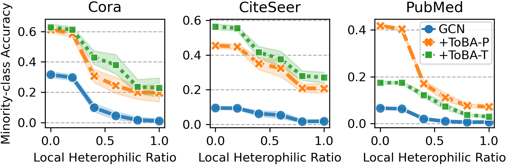
(a) ToBA mitigates AMP in multiple IGL tasks.

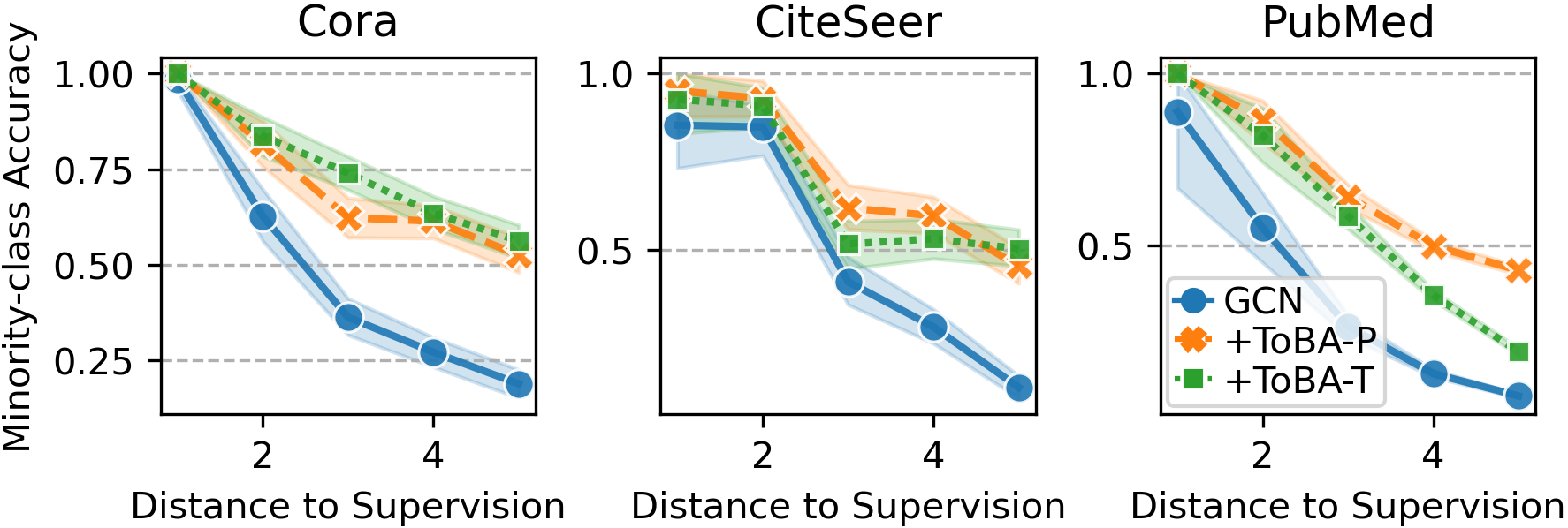
(b) ToBA mitigates DMP in multiple IGL tasks.

Figure 6: ToBA alleviates the bias from both AMP and DMP in IGL via topological augmentation.

On mitigating AMP and DMP (Fig. 6). We further design experiments to verify whether ToBA can effectively handle the topological challenges identified in this paper, i.e., ambivalent and distant message-passing. Specifically, we investigate whether ToBA can improve the prediction accuracy of minority class nodes that are highly influenced by ambivalent/distant message-passing, i.e., high local heterophilic ratios/long distance to supervision signals. Results are shown in Fig. 6 (5 independent runs with GCN classifier, IR=10). As can be observed, ToBA effectively alleviates the negative impact of AMP and DMP and helps node classifiers to achieve better performance in minority classes.

Complexity analysis (Table 3). ToBA introduces $m$ (the number of class) virtual nodes with $\mathcal{O}(n)$ edges. Because of the usage of relative risk in Eq. (3) and the long-tail distribution of node uncertainty, only a small portion of nodes have positive risks with relatively few (empirically around 1-3%) virtual edges introduced. For computation, most of the steps can be executed in parallel in matrix form on a modern GPU with $\mathcal{O}(1)$/$\mathcal{O}(mn+|\mathcal{E}|)$ time/space complexity. The time complexity mostly depends on the topological similarity computation in Eq.(5) which requires the usage of torch.scatter_add

Table 3: Scalability results of ToBA_P/ToBA_T.

Dataset	$\Delta$ Nodes (%)	$\Delta$ Edges (%)	$\Delta$ Time (ms)
Cora	0.258%	2.842%/1.509%	4.61/5.34ms
CiteSeer	0.180%	3.715%/1.081%	4.87/5.84ms
PubMed	0.015%	3.175%/1.464%	6.57/45.558ms
CS	0.082%	1.395%/1.053%	16.44/58.71ms
Physics	0.014%	0.797%/0.527%	30.68/282.85ms

• * Results obtained on an NVIDIA${}^{\text{\textregistered}}$ Tesla V100 32GB GPU.

function with $\mathcal{O}(n)$ time cost. This step is only needed for ToBA_T, thus ToBA_P is usually faster in practice. Table 3 reports the ratio of virtual nodes/edges to the original graph introduced and the running time of ToBA in each iteration on different datasets. We discuss how to further speed up ToBA in practice in Appendix B.1.

5 Related Works

Class-imbalanced learning. Class imbalance is a common problem in many fields of data mining research [15, 16, 24]. Existing solutions for class-imbalanced learning can be categorized into four groups: Resampling methods balance the training set by either discarding majority [18, 28, 29] or synthesizing minority samples [6, 14]. Ensemble techniques [57, 50, 5] train multiple classifiers with various balancing strategies and combine them for inference. Post-hoc correction [20, 45, 32, 17] compensates for minority classes by adjusting the logits during inference. Loss modification methods [18, 25, 9] perform compensation by emphasizing/suppressing minority/majority classes. Generally, these techniques do not consider the graph topology thus have limited performance in IGL.

Imbalanced graph learning. To handle class imbalance in graph data, several methods have been proposed in recent studies [39, 47, 54, 26, 36, 7, 34], we review the most closely related works here. One of the early works GraphSMOTE [54] adopts SMOTE [6] oversampling in the node embedding space to synthesize minority nodes and complements the topology with a learnable edge predictor. A more recent work GraphENS [34] synthesizes the whole ego network through saliency-based ego network mixing to handle the neighbor-overfitting problem. On the other hand, ReNode [7] addresses topology imbalance, i.e., the unequal structure role of labeled nodes in the topology, by down-weighting close-to-boundary labeled nodes. Nevertheless, most studies root from a node-centric perspective and aim to address the imbalance by node/class-wise reweighting or resampling. In this paper, we approach the source of the class-imbalance bias from an under-explored topology-centric perspective, and therefore can further boost existing node-centric techniques.

GNN with heterophilic/long-distance propagation. There have been many discussions on mining from heterophilic graphs [58, 3, 8, 56] and learning with multi-hop propagations [11, 23, 53] in the literature. Heterophilic GNNs usually combine intermediate representations to get better structure-aware features [58]. The recent work GPR-GNN [8] further assigns learnable weights to combine the representations of each layer adaptively via the Generalized PageRank (GPR) technique. For learning with multi-hop propagation, PPNP [11] is a representative method that adopts personalized PageRank to leverage information from a larger neighborhood. However, these works specifically focus on handling the globaly heterophilic graph/long-distance propagation by modifying GNN architecture [58, 8] or aggregation operators [11, 23], and these problems were considered to be orthogonal to IGL. In this work, we present the first study on the impact of AMP and DMP in the context of IGL, and jointly handle them with a model-agnostic augmentation framework that is compatible with other GNN backbones and IGL techniques. Empirical results show that our method can also significantly boost the performance of such advanced GNNs [8, 11] in various IGL tasks.

6 Conclusion

In this paper, we study the class-imbalanced node classification problem from an under-explored topology-centric perspective. We identify two fundamental topological challenges, namely ambivalent and distant message-passing, can exacerbate the predictive bias by aggravating majority-class over-generalization and minority-class misclassification. In light of this, we propose ToBA to identify the nodes that are influenced by such challenges and rectify their learning by dynamic topological augmentation. ToBA is a fast and model-agnostic framework that can be combined with other IGL techniques to further boost their performance and reduce the predictive bias. Extensive experiments validate ToBA’s superior effectiveness, versatility, robustness, and efficiency in various IGL tasks. We hope this work can provide a new perspective for IGL and shed light on future research.

Appendix A Reproducibility

In this section, we describe the detailed experimental settings including (§A.1) data statistics, (§A.2) baseline settings, and (§A.3) evaluation protocols. The source code for implementing and evaluating ToBA and all the IGL baseline methods will be released after the paper is published.

A.1 Data Statistics

As previously described, we adopt 5 benchmark graph datasets: the Cora, CiteSeer, and PubMed citation networks [37], and the CS and Physics coauthor networks [38] to test ToBA on large graphs with more nodes and high-dimensional features. All datasets are publicly available. Table 4 summarizes the dataset statistics.

Table 4: Statistics of datasets.

Dataset	#nodes	#edges	#features	#classes
Cora	2,708	10,556	1,433	7
CiteSeer	3,327	9,104	3,703	6
PubMed	19,717	88,648	500	3
CS	18,333	163,788	6,805	15
Physics	34,493	495,924	8,415	5

We follow previous works [54, 34, 40] to construct and adjust the class imbalanced node classification tasks. For step imbalance, we select half of the classes ($\lfloor m/2\rfloor$) as minority classes and the rest as majority classes. We follow the public split [37] for semi-supervised node classification where each class has 20 training nodes, then randomly remove minority class training nodes until the given imbalance ratio (IR) is met. The imbalance ratio is defined as $\text{IR}=\frac{\#\text{majority training nodes}}{\#\text{minority training nodes}}\in[1,\infty)$, i.e., more imbalanced data has higher IR. For natural imbalance, we simulate the long-tail class imbalance present in real-world data by utilizing a power-law distribution. Specifically, for a given IR, the largest head class have $n_{\text{head}}=\text{IR}$ training nodes, and the smallest tail class have 1 training node. The number of training nodes of the $k$-th class is determined by $n_{k}=\lfloor n_{\text{head}}^{\lambda_{k}}\rfloor,\lambda_{k}=\frac{m-k}{m-1}$. We set the IR (largest class to smallest class) to 50/100 to test ToBA’s robustness under natural and extreme class imbalance. We show the training data distribution under step and natural imbalance in Fig. 7.

Figure 7: Class distribution of training datasets under step and natural imbalance.

A.2 Baseline Settings

To fully validate ToBA’s performance and compatibility with existing IGL techniques and GNN backbones, we include six baseline methods with five popular GNN backbones in our experiments, and combine ToBA with them under all possible combinations. The included IGL baselines can be generally divided into two categories: reweighting-based (i.e., Reweight [18], ReNode [7]) and augmentation-based (i.e., Oversampling [18], SMOTE [6], GraphSMOTE [54], and GraphENS [34]).

• Reweight [18] assigns minority classes with higher misclassification costs (i.e., weights in the loss function) by the inverse of the class frequency in the training set.

• ReNode [7] measures the influence conflict of training nodes, and perform instance-wise node reweighting to alleviate the topology imbalance.

• Oversample [18] augments minority classes with additional synthetic nodes by replication-base oversampling.

• SMOTE [6] synthesizes minority nodes by 1) randomly selecting a seed node, 2) finding its $k$-nearest neighbors in the feature space, and 3) performing linear interpolation between the seed and one of its $k$-nearest neighbors.

• GraphSMOTE [54] extends SMOTE [6] to graph-structured data by 1) performing SMOTE in the low-dimensional embedding space of GNN and 2) utilizing a learnable edge predictor to generate better topology connections for synthetic nodes.

• GraphENS [34] directly synthesize the whole ego network (node with its 1-hop neighbors) for minority classes by similarity-based ego network combining and saliency-based node mixing to prevent neighbor memorization.

We use the public implementations of the baseline methods for a fair comparison. For ReNode [7], we use its transductive version and search hyperparameters among the lower bound of cosine annealing $w_{min}\in\{0.25,0.5,0.75\}$ and upper bound of the cosine annealing $w_{max}\in\{1.25,1.5,1.75\}$ following the original paper. We set the teleport probability of PageRank $\alpha=0.15$ as given by the default setting in the released implementation. As Oversample [9] and SMOTE [6] were not proposed to handle graph data, we adopt their enhanced versions provided by GraphSMOTE [54], which also duplicate the edges from the seed nodes to the synthesized nodes in order to connect them to the graph. For GraphSMOTE [54], we use the version that predicts edges with binary values as it performs better than the variant with continuous edge predictions in many datasets. For GraphENS [34], we follow the settings in the paper: $\text{Beta}(2,2)$ distribution is used to sample $\lambda$, the feature masking hyperparameter $k$ and temperature $\tau$ are tuned among $\{1,5,10\}$ and $\{1,2\}$, and the number of warmup epochs is set to 5.

We use Pytorch [35] and PyG [10] to implement all five GNN backbones used in this paper, i.e., GCN [48], GAT [46], GraphSAGE [12], PPNP [11], and GPRGNN [8]. Most of our settings are aligned with prevailing works [34, 7, 40] to obtain fair and comparable results. Specifically, we implement all GNNs’ convolution layer with ReLU activation and dropout [42] with a dropping rate of 0.5 before the last layer. For GAT, we set the number of attention heads to 4. For PPNP and GPRGNN, we follow the best setting in the original paper and use 2 PPNP/GPR_prop convolution layers with 64 hidden units. Note that GraphENS’s official implementation requires modifying the graph convolution for resampling and thus cannot be directly combined with PPNP and GPRGNN. The teleport probability = 0.1 and the number of power iteration steps K = 10. We search for the best architecture for other backbones from #layers $l\in\{1,2,3\}$ and hidden dimension $d\in\{64,128,256\}$ based on the average of validation accuracy and F1 score. We train each GNN for 2,000 epochs using Adam optimizer [22] with an initial learning rate of 0.01. To achieve better convergence, we follow [34] to use 5e-4 weight decay and adopt the ReduceLROnPlateau scheduler in Pytorch, which reduces the learning rate by half if the validation loss does not improve for 100 epochs.

A.3 Evaluation Protocol

To evaluate the predictive performance on class-imbalanced data, we use two balanced metrics, i.e., balanced accuracy (BAcc.) and macro-averaged F1 score (Macro-F1). They compute accuracy/F1-score for each class independently and use the unweighted average mean as the final score, i.e., BAcc. $=\frac{1}{m}\sum_{i=1}^{m}Acc(c_{i})$, Macro-F1 $=\frac{1}{m}\sum_{i=1}^{m}F1(c_{i})$. Additionally, we use performance parity to evaluate the level of model predictive bias. Formally, let $Acc(c_{i})$ be the classification accuracy of class $c_{i}$, the disparity is defined as the standard deviation of the accuracy scores of all classes, i.e., $\sqrt{\frac{1}{m}\sum_{i=1}^{m}(Acc(c_{i})-\textit{BAcc.})^{2}}$. All the experiments are conducted on a Linux server with Intel${}^{\text{\textregistered}}$ Xeon${}^{\text{\textregistered}}$ Gold 6240R CPU and NVIDIA${}^{\text{\textregistered}}$ Tesla V100 32GB GPU.

Appendix B Additional Results and Discussions

In this section, we discuss how to further speed up ToBA in practice (§B.1) as well as the limitation and future works (§B.2). Finally, we provide the full, detailed results of Table 4 and 2 (§B.3).

B.1 On the Further Speedup of ToBA

As stated in the paper, thanks to its simple and efficient design, ToBA can be integrated into the GNN training process to perform dynamic topology augmentation based on the training state. By default, we run ToBA in every iteration of GNN training, i.e., the granularity of applying ToBA is 1, as described in Alg. 1. However, we note that in practice, this granularity can be increased to further reduce the cost of applying ToBA. This operation can result in a significant linear speedup ratio: setting the granularity to $N$ reduces the computational overhead of ToBA to $1/N$ of the original (i.e., $N$x speedup ratio), with minor performance degradation. This could be helpful for scaling ToBA to large-scale graphs in practice. In this section, we design experiments to validate the influence of different ToBA granularity (i.e., the number of iterations per each use of ToBA) in real-world IGL tasks. We set the granularity to 1/5/10/50/100 and test the performance of ToBA_T with a vanilla GCN classifier on the Cora/CiteSeer/PubMed dataset with an imbalance ratio of 10. Fig. 8 shows the empirical results from 10 independent runs. The red horizontal line in each subfigure represents the baseline (vanilla GCN) performance. It can be observed that setting a larger ToBA granularity is an effective way to further speed up ToBA in practice. The performance drop of adopting this trick is relatively minor, especially considering the significant linear speedup ratio it brings. The predictive performance boost brought by ToBA is still significant even with a large granularity at 100 (i.e., with 100x ToBA speedup).

(a) Influence of ToBA granularity on BAcc.

(b) Influence of ToBA granularity on Macro-F1.

Figure 8: Influence of the ToBA granularity (i.e., the number of iterations per each use of ToBA). Note that this brings a linear speedup ratio in practice, e.g., granularity = 100 $\Leftrightarrow$ 100x speedup.

B.2 Limitations and Future Works

One potential limitation of the proposed ToBA framework is its reliance on exploiting model prediction for risk and similarity estimation. This strategy may not provide accurate estimation when the model itself exhibits extremely poor predictive performance. However, this rarely occurs in practice and can be prevented by more careful fine-tuning of parameters and model architectures. In addition to this, as described in Section 3, we adopt several fast measures to estimate node uncertainty, prediction risk, and node-class similarity for the sake of efficiency. Other techniques for such purposes (e.g., deterministic[27, 55]/Bayesian[52, 13]/Jackknife[21] uncertainty estimation) can be easily integrated into the proposed ToBA framework, although the computational efficiency might be a major bottleneck. How to exploit alternative uncertainty/risk measures while retaining computational efficiency is an interesting future direction. Finally, in this work, we aim to mitigate the negative influence caused by heterophilic connections for a broad range of GNN models including those originally designed based on homophily assumption. How to extend ToBA to graphs with high heterophily is another interesting future direction. A possible solution is to consider multi-scale node neighborhoods (e.g., by combining intermediate representations [58, 8]) to achieve better structure-aware augmentation. Investigating this and adaptive topological augmentation for graphs with arbitrary homophily would be an exciting future research direction.

B.3 Additional results

Due to space limitation, we report the key results of our experiments in Table 4 and 2. We now provide complete results with the standard error of 5 independent runs. Specifically, Table B.3 & B.3 & B.3 complement Table 4, and Table 8 complements Table 2. The results indicate that ToBA can consistently boost various IGL baselines with all GNN backbones, performance metrics, as well as different types and levels of class imbalance, which aligns with our conclusions in the paper.

Table 5: Balanced accuracy of combining ToBA with 6 IGL baselines $\times$ 5 GNN backbones.

Dataset (IR=10)

Cora

CiteSeer

PubMed

Metric: BAcc.$\uparrow$

Base

+ ToBAP

+ ToBAT

Base

+ ToBAP

+ ToBAT

Base

+ ToBAP

+ ToBAT

GCN

Vanilla

61.56$\pm$1.24

65.54$\pm$1.25

69.80$\pm$1.30

37.62$\pm$1.61

52.65$\pm$1.08

55.37$\pm$1.39

64.23$\pm$1.55

68.62$\pm$0.77

67.57$\pm$3.22

Reweight

67.65$\pm$0.64

70.97$\pm$1.28

72.14$\pm$0.72

42.49$\pm$2.66

57.91$\pm$0.98

58.36$\pm$1.09

71.20$\pm$2.33

74.19$\pm$1.12

73.37$\pm$0.96

ReNode

66.60$\pm$1.33

71.37$\pm$0.62

71.84$\pm$1.25

42.57$\pm$1.05

57.47$\pm$0.62

59.28$\pm$0.59

71.52$\pm$2.16

73.20$\pm$0.71

72.53$\pm$1.62

Resample

59.48$\pm$1.53

72.51$\pm$0.68

74.24$\pm$0.91

39.15$\pm$2.05

57.90$\pm$0.33

58.78$\pm$1.44

64.97$\pm$1.94

72.53$\pm$0.85

72.87$\pm$1.16

SMOTE

58.27$\pm$1.05

72.16$\pm$0.53

73.89$\pm$1.06

39.27$\pm$1.90

60.06$\pm$0.81

61.97$\pm$1.19

64.41$\pm$1.95

73.17$\pm$0.84

73.13$\pm$0.77

GSMOTE

67.99$\pm$1.37

68.52$\pm$0.81

71.55$\pm$0.50

45.05$\pm$1.95

57.68$\pm$1.03

57.65$\pm$1.18

73.99$\pm$0.88

73.09$\pm$1.30

76.57$\pm$0.42

GENS

70.12$\pm$0.43

72.22$\pm$0.57

72.58$\pm$0.58

56.01$\pm$1.17

60.60$\pm$0.63

62.67$\pm$0.42

73.66$\pm$1.04

76.11$\pm$0.60

76.91$\pm$1.03

2-11[1pt/1pt]

Best

70.12

72.51

74.24

56.01

60.60

62.67

73.99

76.11

76.91

GAT

Vanilla

61.53$\pm$1.13

66.27$\pm$0.83

70.13$\pm$1.07

39.25$\pm$1.84

55.66$\pm$1.23

60.34$\pm$1.66

65.46$\pm$0.69

73.19$\pm$0.86

74.75$\pm$1.18

Reweight

66.94$\pm$1.24

71.80$\pm$0.48

71.61$\pm$0.85

41.29$\pm$3.39

59.33$\pm$0.51

61.23$\pm$0.99

68.37$\pm$1.41

75.30$\pm$1.07

74.52$\pm$1.14

ReNode

66.81$\pm$0.98

72.14$\pm$1.24

70.31$\pm$1.38

43.25$\pm$1.78

58.26$\pm$1.98

59.05$\pm$0.88

71.18$\pm$2.13

75.55$\pm$1.01

75.22$\pm$0.84

Resample

57.76$\pm$1.73

71.90$\pm$0.88

73.29$\pm$1.08

35.97$\pm$1.42

60.10$\pm$1.26

60.33$\pm$0.75

65.14$\pm$0.86

73.27$\pm$0.61

73.89$\pm$0.40

SMOTE

58.81$\pm$0.64

70.50$\pm$0.44

72.19$\pm$0.75

36.95$\pm$1.86

60.59$\pm$1.19

62.36$\pm$1.18

64.81$\pm$1.47

73.90$\pm$0.68

74.08$\pm$0.51

GSMOTE

64.68$\pm$1.02

69.29$\pm$1.82

71.14$\pm$0.96

41.82$\pm$1.14

56.11$\pm$1.23

57.71$\pm$2.58

68.72$\pm$1.69

74.65$\pm$0.65

74.41$\pm$1.57

GENS

69.76$\pm$0.45

70.63$\pm$0.40

71.02$\pm$1.22

51.50$\pm$2.21

60.95$\pm$1.51

63.49$\pm$0.75

73.13$\pm$1.18

74.34$\pm$0.35

75.65$\pm$0.82

2-11[1pt/1pt]

Best

69.76

72.14

73.29

51.50

60.95

63.49

73.13

75.55

75.65

SAGE

Vanilla

59.17$\pm$1.23

66.24$\pm$0.92

66.53$\pm$0.80

42.96$\pm$0.28

54.99$\pm$2.51

53.18$\pm$2.90

67.56$\pm$0.84

75.31$\pm$0.93

77.38$\pm$0.68

Reweight

63.76$\pm$0.89

70.15$\pm$1.15

71.14$\pm$0.84

45.91$\pm$2.05

57.95$\pm$0.73

55.90$\pm$0.93

68.03$\pm$1.69

74.56$\pm$0.41

75.39$\pm$0.38

ReNode

65.32$\pm$1.07

71.31$\pm$1.29

71.54$\pm$0.85

48.55$\pm$2.31

56.32$\pm$0.40

56.49$\pm$1.73

69.08$\pm$2.04

74.24$\pm$0.20

75.28$\pm$0.69

Resample

57.77$\pm$1.35

71.24$\pm$1.08

73.01$\pm$1.02

39.37$\pm$1.40

61.41$\pm$1.11

61.93$\pm$1.40

69.22$\pm$1.28

74.91$\pm$1.09

75.80$\pm$0.39

SMOTE

58.81$\pm$1.97

70.31$\pm$1.35

73.02$\pm$2.29

38.42$\pm$1.69

64.14$\pm$0.75

66.35$\pm$0.70

64.96$\pm$1.56

74.59$\pm$0.96

77.31$\pm$0.45

GSMOTE

61.57$\pm$1.78

69.88$\pm$0.96

72.28$\pm$1.48

42.21$\pm$2.12

60.91$\pm$1.33

62.32$\pm$1.06

71.55$\pm$0.64

74.74$\pm$0.81

76.14$\pm$0.21

GENS

68.84$\pm$0.41

69.78$\pm$1.18

71.92$\pm$0.71

52.57$\pm$1.78

64.36$\pm$0.68

63.84$\pm$0.68

71.38$\pm$0.99

75.89$\pm$1.17

76.46$\pm$1.29

2-11[1pt/1pt]

Best

68.84

71.31

73.02

52.57

64.36

66.35

71.55

75.89

77.38

PPNP

Vanilla

55.37$\pm$1.65

58.13$\pm$1.69

61.71$\pm$1.66

35.69$\pm$0.14

35.68$\pm$0.15

36.02$\pm$0.25

59.30$\pm$0.50

55.62$\pm$0.31

57.82$\pm$0.29

Reweight

72.62$\pm$0.47

73.62$\pm$0.89

72.51$\pm$0.87

50.88$\pm$3.64

63.54$\pm$1.02

65.57$\pm$1.11

72.00$\pm$0.81

72.15$\pm$0.60

71.22$\pm$1.10

ReNode

73.74$\pm$1.12

75.02$\pm$1.54

72.15$\pm$0.76

50.50$\pm$3.51

63.73$\pm$0.54

65.13$\pm$0.40

72.76$\pm$1.37

71.54$\pm$0.96

71.88$\pm$0.70

Resample

65.78$\pm$1.72

73.14$\pm$0.94

73.57$\pm$0.92

40.79$\pm$1.87

66.54$\pm$0.49

59.51$\pm$4.16

67.74$\pm$1.94

72.25$\pm$0.81

74.41$\pm$0.95

SMOTE

65.34$\pm$1.68

73.18$\pm$1.02

72.88$\pm$0.90

40.79$\pm$2.05

66.62$\pm$0.33

58.82$\pm$4.59

67.24$\pm$2.10

72.67$\pm$1.65

73.33$\pm$1.37

GSMOTE

71.13$\pm$0.72

73.37$\pm$0.82

73.78$\pm$0.71

45.37$\pm$2.75

64.95$\pm$0.11

62.95$\pm$2.58

69.57$\pm$2.20

73.37$\pm$0.95

74.90$\pm$1.27

2-11[1pt/1pt]

Best

73.74

75.02

73.78

50.88

66.62

65.57

72.76

73.37

74.90

GPRGNN

Vanilla

67.97$\pm$0.51

71.99$\pm$1.14

73.38$\pm$1.18

42.31$\pm$2.16

55.85$\pm$0.89

58.82$\pm$1.91

67.04$\pm$1.82

57.92$\pm$0.45

77.49$\pm$1.15

Reweight

72.15$\pm$0.57

72.90$\pm$1.33

73.22$\pm$0.55

53.22$\pm$2.89

59.78$\pm$0.76

61.00$\pm$1.82

73.35$\pm$1.07

75.22$\pm$1.02

76.86$\pm$0.76

ReNode

73.38$\pm$0.67

73.71$\pm$0.57

73.93$\pm$1.60

54.66$\pm$2.82

59.69$\pm$0.73

60.34$\pm$1.31

73.56$\pm$0.98

75.69$\pm$1.10

76.25$\pm$0.67

Resample

67.00$\pm$1.33

72.94$\pm$1.02

74.89$\pm$0.86

42.27$\pm$2.15

64.16$\pm$0.62

63.89$\pm$0.98

70.42$\pm$1.51

73.79$\pm$0.83

75.31$\pm$0.54

SMOTE

66.99$\pm$1.33

74.01$\pm$1.51

74.41$\pm$1.05

40.97$\pm$2.02

63.88$\pm$0.55

62.60$\pm$1.72

70.29$\pm$1.47

73.89$\pm$0.69

75.48$\pm$1.02

GSMOTE

70.94$\pm$0.57

73.63$\pm$1.25

74.02$\pm$0.90

48.01$\pm$3.28

63.03$\pm$0.92

61.68$\pm$0.86

71.51$\pm$1.91

72.16$\pm$0.58

74.77$\pm$0.83

2-11[1pt/1pt]

Best

73.38

74.01

74.89

54.66

64.16

63.89

73.56

75.69

77.49

Table 6: Macro-F1 score of combining ToBA with 6 IGL baselines $\times$ 5 GNN backbones.

Dataset (IR=10)

Cora

CiteSeer

PubMed

Metric: Macro-F1$\uparrow$

Base

+ ToBAP

+ ToBAT

Base

+ ToBAP

+ ToBAT

Base

+ ToBAP

+ ToBAT

GCN

Vanilla

60.10$\pm$1.53

63.28$\pm$1.07

68.68$\pm$1.49

28.05$\pm$2.53

51.55$\pm$1.28

54.94$\pm$1.44

55.09$\pm$2.48

67.16$\pm$1.53

64.40$\pm$3.68

Reweight

67.85$\pm$0.62

69.41$\pm$1.01

70.31$\pm$0.82

36.59$\pm$3.66

56.84$\pm$1.06

57.54$\pm$1.08

67.07$\pm$3.42

72.94$\pm$0.81

73.24$\pm$0.90

ReNode

66.66$\pm$1.59

69.79$\pm$0.79

70.59$\pm$1.25

34.64$\pm$1.54

56.69$\pm$0.64

58.07$\pm$0.77

67.86$\pm$3.99

72.61$\pm$0.41

72.25$\pm$0.89

Resample

57.34$\pm$2.27

71.36$\pm$0.39

72.82$\pm$1.13

29.73$\pm$2.77

57.17$\pm$0.48

58.03$\pm$1.42

56.74$\pm$3.54

71.19$\pm$0.83

73.13$\pm$1.33

SMOTE

55.65$\pm$1.62

71.04$\pm$0.16

72.82$\pm$0.86

29.39$\pm$2.81

59.53$\pm$0.88

61.53$\pm$1.24

56.14$\pm$3.74

71.72$\pm$0.60

72.83$\pm$1.20

GSMOTE

68.01$\pm$1.67

67.60$\pm$1.00

70.28$\pm$0.48

40.07$\pm$3.02

56.64$\pm$1.09

56.25$\pm$1.50

70.60$\pm$1.17

72.95$\pm$1.39

75.70$\pm$0.35

GENS

69.96$\pm$0.29

71.62$\pm$0.64

72.28$\pm$0.65

54.45$\pm$1.69

59.89$\pm$0.68

62.46$\pm$0.43

71.28$\pm$1.84

75.77$\pm$0.55

76.86$\pm$0.93

2-11[1pt/1pt]

Best

69.96

71.62

72.82

54.45

59.89

62.46

71.28

75.77

76.86

GAT

Vanilla

60.71$\pm$1.61

64.27$\pm$0.95

68.93$\pm$0.79

31.12$\pm$3.15

54.71$\pm$1.18

59.42$\pm$1.55

57.32$\pm$1.55

71.27$\pm$1.11

74.03$\pm$1.08

Reweight

66.49$\pm$1.34

69.84$\pm$0.91

69.79$\pm$0.77

34.94$\pm$4.09

58.53$\pm$0.68

60.28$\pm$1.12

63.82$\pm$1.60

75.13$\pm$1.13

73.88$\pm$1.38

ReNode

67.27$\pm$1.23

70.61$\pm$0.83

68.24$\pm$1.48

37.72$\pm$2.61

57.64$\pm$2.11

58.57$\pm$0.75

67.38$\pm$3.22

74.88$\pm$0.99

74.96$\pm$1.18

Resample

55.36$\pm$2.47

70.87$\pm$0.94

72.31$\pm$1.07

25.71$\pm$1.97

59.77$\pm$1.31

59.66$\pm$0.95

57.24$\pm$1.54

72.53$\pm$0.66

73.09$\pm$0.83

SMOTE

57.49$\pm$0.60

69.68$\pm$0.66

71.74$\pm$1.03

26.05$\pm$2.30

59.83$\pm$1.33

61.75$\pm$1.30

55.66$\pm$2.76

73.33$\pm$1.00

73.30$\pm$0.16

GSMOTE

64.34$\pm$1.69

68.23$\pm$1.80

69.77$\pm$1.08

35.07$\pm$1.77

55.86$\pm$1.10

57.13$\pm$2.69

63.35$\pm$2.92

74.23$\pm$0.84

73.34$\pm$2.06

GENS

69.96$\pm$0.62

69.83$\pm$0.41

70.71$\pm$1.16

48.34$\pm$2.19

60.04$\pm$1.85

62.55$\pm$0.86

71.78$\pm$1.19

72.69$\pm$0.84

74.42$\pm$1.12

2-11[1pt/1pt]

Best

69.96

70.87

72.31

48.34

60.04

62.55

71.78

75.13

74.96

SAGE

Vanilla

57.36$\pm$1.77

64.90$\pm$0.87

65.61$\pm$0.97

36.07$\pm$1.06

54.76$\pm$2.47

51.86$\pm$3.25

63.75$\pm$1.24

74.35$\pm$0.74

76.92$\pm$0.63

Reweight

63.72$\pm$1.10

69.06$\pm$0.90

69.59$\pm$0.53

39.64$\pm$2.57

57.17$\pm$0.76

54.83$\pm$0.74

62.83$\pm$2.57

73.88$\pm$0.40

75.42$\pm$0.48

ReNode

65.59$\pm$1.44

69.99$\pm$1.35

69.86$\pm$1.27

44.20$\pm$3.68

55.41$\pm$0.48

55.78$\pm$1.63

64.97$\pm$3.00

74.33$\pm$0.20

74.88$\pm$0.53

Resample

55.29$\pm$2.12

70.40$\pm$1.11

71.49$\pm$0.79

30.14$\pm$2.20

60.71$\pm$1.25

61.29$\pm$1.48

65.23$\pm$2.26

74.28$\pm$0.96

75.48$\pm$0.44

SMOTE

56.72$\pm$2.69

69.42$\pm$1.29

71.71$\pm$1.94

29.22$\pm$2.33

63.61$\pm$0.87

65.91$\pm$0.68

57.60$\pm$3.22

72.98$\pm$0.69

76.45$\pm$0.77

GSMOTE

59.44$\pm$2.25

69.10$\pm$0.95

71.30$\pm$1.47

34.86$\pm$3.46

60.53$\pm$1.27

61.96$\pm$1.12

67.23$\pm$0.61

74.36$\pm$1.02

75.68$\pm$0.31

GENS

68.23$\pm$0.72

69.76$\pm$0.95

71.11$\pm$0.81

51.05$\pm$2.03

63.87$\pm$0.82

63.41$\pm$0.57

70.06$\pm$0.86

75.33$\pm$1.46

76.01$\pm$1.14

2-11[1pt/1pt]

Best

68.23

70.40

71.71

51.05

63.87

65.91

70.06

75.33

76.92

PPNP

Vanilla

50.39$\pm$2.81

54.19$\pm$2.58

59.99$\pm$2.49

22.21$\pm$0.13

22.54$\pm$0.25

22.89$\pm$0.22

44.50$\pm$0.21

44.67$\pm$0.07

44.59$\pm$0.06

Reweight

72.63$\pm$0.53

72.71$\pm$0.60

70.61$\pm$0.65

45.25$\pm$4.85

63.08$\pm$1.03

65.20$\pm$1.20

69.53$\pm$1.14

72.24$\pm$0.58

72.26$\pm$0.80

ReNode

73.67$\pm$0.98

73.67$\pm$1.18

69.79$\pm$0.72

44.91$\pm$4.99

62.97$\pm$0.78

64.47$\pm$0.40

70.65$\pm$1.66

72.33$\pm$0.90

72.18$\pm$0.55

Resample

65.20$\pm$2.08

72.25$\pm$0.82

72.72$\pm$0.97

31.04$\pm$2.76

66.06$\pm$0.54

54.57$\pm$6.08

62.42$\pm$3.62

72.32$\pm$0.93

74.27$\pm$1.08

SMOTE

64.70$\pm$2.06

72.90$\pm$0.83

72.31$\pm$0.94

30.90$\pm$2.86

66.18$\pm$0.37

53.90$\pm$6.26

61.83$\pm$3.65

72.55$\pm$1.61

73.87$\pm$1.37

GSMOTE

71.20$\pm$0.67

73.02$\pm$0.74

73.22$\pm$0.92

37.90$\pm$4.29

64.56$\pm$0.18

60.41$\pm$3.84

65.65$\pm$3.06

72.54$\pm$0.85

74.61$\pm$1.36

2-11[1pt/1pt]

Best

73.67

73.67

73.22

45.25

66.18

65.20

70.65

72.55

74.61

GPRGNN

Vanilla

67.86$\pm$0.79

70.80$\pm$1.16

72.32$\pm$1.18

35.00$\pm$2.96

55.06$\pm$0.89

56.31$\pm$2.87

59.01$\pm$3.62

50.12$\pm$1.46

77.62$\pm$1.04

Reweight

71.66$\pm$0.85

70.46$\pm$0.98

71.24$\pm$0.49

49.19$\pm$3.61

59.11$\pm$0.73

60.30$\pm$2.04

71.18$\pm$0.95

75.47$\pm$0.90

77.01$\pm$0.52

ReNode

73.08$\pm$0.66

71.52$\pm$0.50

71.72$\pm$1.51

50.34$\pm$3.18

59.10$\pm$0.75

58.94$\pm$1.36

71.45$\pm$1.19

75.08$\pm$1.06

75.76$\pm$0.84

Resample

66.42$\pm$1.65

71.70$\pm$0.86

73.54$\pm$0.83

32.60$\pm$2.71

63.59$\pm$0.65

63.12$\pm$1.06

66.58$\pm$2.08

73.66$\pm$0.86

75.42$\pm$0.35

SMOTE

66.43$\pm$1.74

72.89$\pm$1.23

73.47$\pm$1.12

31.38$\pm$2.70

63.41$\pm$0.55

61.23$\pm$2.59

66.78$\pm$1.97

73.98$\pm$0.70

75.63$\pm$0.91

GSMOTE

70.87$\pm$0.53

72.53$\pm$0.85

73.12$\pm$0.95

42.82$\pm$4.52

62.09$\pm$1.04

60.82$\pm$0.88

67.93$\pm$3.01

72.72$\pm$0.72

74.66$\pm$0.74

2-11[1pt/1pt]

Best

73.08

72.89

73.54

50.34

63.59

63.12

71.45

75.47

77.62

Table 7: Performance disparity of combining ToBA with 6 IGL baselines $\times$ 5 GNN backbones.

Dataset (IR=10)

Cora

CiteSeer

PubMed

Metric: Disparity$\downarrow$

Base

+ ToBAP

+ ToBAT

Base

+ ToBAP

+ ToBAT

Base

+ ToBAP

+ ToBAT

GCN

Vanilla

27.88$\pm$1.79

21.27$\pm$1.76

18.49$\pm$2.68

29.93$\pm$1.38

13.82$\pm$2.06

13.93$\pm$0.80

34.73$\pm$2.14

9.23$\pm$2.78

21.81$\pm$4.51

Reweight

22.29$\pm$1.41

14.43$\pm$2.51

18.32$\pm$2.20

25.47$\pm$1.78

19.10$\pm$1.48

22.64$\pm$0.79

19.33$\pm$5.26

10.21$\pm$1.58

5.88$\pm$0.83

ReNode

22.88$\pm$1.64

14.65$\pm$2.07

17.00$\pm$2.13

30.31$\pm$1.51

20.22$\pm$0.88

22.99$\pm$1.09

18.14$\pm$5.79

12.99$\pm$1.57

10.96$\pm$1.92

Resample

31.57$\pm$1.85

15.13$\pm$2.14

15.25$\pm$2.79

31.00$\pm$1.32

16.30$\pm$1.89

20.79$\pm$0.43

30.90$\pm$5.67

11.63$\pm$3.20

7.82$\pm$0.80

SMOTE

33.32$\pm$1.38

16.33$\pm$1.12

17.95$\pm$2.50

32.61$\pm$1.45

17.27$\pm$0.86

18.25$\pm$0.89

31.79$\pm$5.21

10.56$\pm$1.82

11.66$\pm$2.58

GSMOTE

21.78$\pm$1.79

17.90$\pm$2.75

18.44$\pm$2.20

22.64$\pm$2.69

21.37$\pm$1.25

21.01$\pm$1.45

15.87$\pm$2.34

3.35$\pm$1.08

5.83$\pm$1.27

GENS

20.04$\pm$1.12

16.98$\pm$3.02

18.02$\pm$2.23

16.95$\pm$2.64

14.94$\pm$0.75

15.54$\pm$0.60

11.93$\pm$3.46

5.95$\pm$1.85

5.15$\pm$0.80

2-11[1pt/1pt]

Best

20.04

14.43

15.25

16.95

13.82

13.93

11.93

3.35

5.15

GAT

Vanilla

27.38$\pm$1.71

19.23$\pm$0.80

17.97$\pm$2.65

28.32$\pm$2.07

15.62$\pm$0.77

15.90$\pm$0.95

30.94$\pm$1.27

10.77$\pm$2.04

8.51$\pm$2.48

Reweight

22.90$\pm$1.67

16.44$\pm$2.71

17.32$\pm$2.83

30.27$\pm$1.26

18.64$\pm$1.30

20.83$\pm$1.06

24.92$\pm$1.88

3.01$\pm$0.96

5.44$\pm$1.33

ReNode

23.13$\pm$1.54

15.05$\pm$1.59

18.96$\pm$1.65

25.21$\pm$1.85

20.48$\pm$0.82

20.51$\pm$0.49

18.15$\pm$4.37

4.77$\pm$1.22

6.17$\pm$0.42

Resample

32.73$\pm$2.12

17.87$\pm$2.04

17.64$\pm$2.57

32.59$\pm$0.89

17.76$\pm$1.79

18.73$\pm$1.02

31.67$\pm$0.98

6.18$\pm$1.35

4.58$\pm$1.14

SMOTE

31.17$\pm$0.69

18.40$\pm$1.03

18.26$\pm$1.87

33.32$\pm$0.88

10.68$\pm$0.68

13.24$\pm$1.12

32.79$\pm$2.13

8.14$\pm$2.00

7.56$\pm$1.05

GSMOTE

24.84$\pm$1.60

15.48$\pm$2.08

18.23$\pm$2.00

26.74$\pm$1.53

18.34$\pm$1.64

19.76$\pm$0.42

24.50$\pm$2.78

5.12$\pm$1.38

8.54$\pm$2.03

GENS

20.08$\pm$1.56

17.75$\pm$2.40

17.88$\pm$2.50

26.49$\pm$1.18

12.89$\pm$0.77

15.09$\pm$0.95

10.29$\pm$2.75

7.83$\pm$2.27

7.55$\pm$2.38

2-11[1pt/1pt]

Best

20.08

15.05

17.32

25.21

10.68

13.24

10.29

3.01

4.58

SAGE

Vanilla

29.94$\pm$1.75

18.62$\pm$2.13

19.49$\pm$1.67

26.75$\pm$1.58

14.56$\pm$1.16

18.13$\pm$1.32

21.09$\pm$3.43

10.96$\pm$1.99

4.09$\pm$1.17

Reweight

25.61$\pm$1.60

15.24$\pm$2.66

17.54$\pm$2.45

29.95$\pm$1.83

19.05$\pm$1.60

22.94$\pm$0.49

25.47$\pm$3.49

3.35$\pm$0.72

8.09$\pm$0.19

ReNode

24.12$\pm$1.73

13.32$\pm$3.03

15.45$\pm$2.41

22.41$\pm$4.31

22.20$\pm$0.97

22.75$\pm$0.87

22.92$\pm$4.36

7.63$\pm$1.23

5.77$\pm$1.55

Resample

31.66$\pm$1.47

15.77$\pm$2.75

15.08$\pm$2.74

30.29$\pm$1.16

18.72$\pm$0.90

18.48$\pm$2.00

21.41$\pm$2.88

4.68$\pm$1.42

4.76$\pm$1.09

SMOTE

30.86$\pm$2.64

17.30$\pm$2.09

14.87$\pm$3.23

32.07$\pm$1.00

13.17$\pm$1.33

12.78$\pm$0.43

31.62$\pm$2.86

13.88$\pm$1.44

11.63$\pm$2.28

GSMOTE

27.71$\pm$1.86

17.28$\pm$2.25

16.10$\pm$2.94

28.77$\pm$2.61

18.69$\pm$0.76

18.05$\pm$1.21

20.10$\pm$0.90

5.37$\pm$1.21

4.64$\pm$1.61

GENS

19.81$\pm$1.65

17.50$\pm$2.05

17.63$\pm$2.11

19.76$\pm$2.07

15.99$\pm$0.81

16.99$\pm$0.85

11.76$\pm$2.91

7.63$\pm$1.51

8.31$\pm$1.64

2-11[1pt/1pt]

Best

19.81

13.32

14.87

19.76

13.17

12.78

11.76

3.35

4.09

PPNP

Vanilla

38.32$\pm$1.94

35.50$\pm$2.10

32.18$\pm$1.68

36.82$\pm$0.10

36.67$\pm$0.25

36.83$\pm$0.36

42.13$\pm$0.27

40.45$\pm$0.11

41.34$\pm$0.16

Reweight

19.83$\pm$1.46

17.33$\pm$2.88

18.46$\pm$2.42

26.19$\pm$2.93

20.96$\pm$0.58

19.38$\pm$0.72

16.96$\pm$2.84

8.04$\pm$1.94

9.13$\pm$1.05

ReNode

18.09$\pm$2.52

16.87$\pm$2.95

19.47$\pm$2.00

25.95$\pm$3.66

22.09$\pm$1.43

20.42$\pm$1.57

14.49$\pm$3.81

10.25$\pm$1.93

3.95$\pm$1.02

Resample

27.28$\pm$2.13

18.37$\pm$2.34

18.72$\pm$2.32

32.71$\pm$1.23

15.87$\pm$1.02

23.72$\pm$4.14

25.86$\pm$4.38

13.60$\pm$1.68

9.49$\pm$1.65

SMOTE

27.86$\pm$1.78

18.61$\pm$2.35

19.42$\pm$1.81

33.26$\pm$1.10

14.91$\pm$0.93

22.90$\pm$4.49

26.37$\pm$4.47

13.37$\pm$1.97

8.70$\pm$2.29

GSMOTE

20.98$\pm$1.45

18.19$\pm$2.59

18.55$\pm$2.28

29.39$\pm$2.20

16.49$\pm$1.12

19.19$\pm$3.44

22.32$\pm$4.21

11.53$\pm$3.00

10.69$\pm$2.27

2-11[1pt/1pt]

Best

18.09

16.87

18.46

25.95

14.91

19.19

14.49

8.04

3.95

GPRGNN

Vanilla

22.96$\pm$1.20

18.12$\pm$2.29

17.00$\pm$2.98

27.57$\pm$1.32

17.10$\pm$1.17

20.94$\pm$2.58

29.94$\pm$3.68

36.57$\pm$1.46

5.30$\pm$0.91

Reweight

20.94$\pm$1.21

17.83$\pm$2.82

19.67$\pm$1.81

22.43$\pm$2.39

21.52$\pm$1.06

20.03$\pm$1.81

16.12$\pm$1.84

7.54$\pm$0.49

5.48$\pm$1.49

ReNode

18.84$\pm$2.19

16.78$\pm$2.53

17.89$\pm$2.96

24.14$\pm$1.47

19.84$\pm$1.79

22.83$\pm$1.40

14.40$\pm$3.18

9.75$\pm$2.20

6.61$\pm$1.47

Resample

25.62$\pm$1.80

19.23$\pm$2.26

17.61$\pm$2.77

33.08$\pm$0.66

17.04$\pm$0.78

15.98$\pm$0.93

22.59$\pm$2.75

7.62$\pm$2.50

7.76$\pm$0.85

SMOTE

25.44$\pm$1.88

16.97$\pm$3.19

17.38$\pm$2.78

32.85$\pm$0.95

15.09$\pm$1.23

16.85$\pm$2.51

21.35$\pm$2.76

9.41$\pm$2.67

6.09$\pm$0.62

GSMOTE

21.23$\pm$1.48

18.02$\pm$2.62

19.06$\pm$2.28

24.21$\pm$3.06

14.83$\pm$0.95

19.11$\pm$1.73

20.08$\pm$3.77

5.99$\pm$1.49

8.27$\pm$0.75

2-11[1pt/1pt]

Best

18.84

16.78

17.00

22.43

14.83

15.98

14.40

5.99

5.30

Table 8: Performance of ToBA under varying types and levels of class imbalance. For each setting, we report the relative gain over base and mark the best/second-best score in bold/underlined.

Dataset		Cora		CiteSeer		PubMed		CS		Physics
Step IR		10	20	10	20	10	20	10	20	10	20
BAcc.$\uparrow$	Base	61.6	52.7	37.6	34.2	64.2	60.8	75.4	65.3	80.1	67.7
	+ ToBA	69.8+13.4%	71.3+35.2%	55.4+47.2%	51.3+49.9%	68.6+6.8%	63.3+4.1%	82.6+9.6%	79.9+22.2%	87.6+9.4%	88.0+29.9%
	BestIGL	70.1+13.9%	66.5+26.2%	56.0+48.9%	47.2+38.0%	74.0+15.2%	71.1+17.0%	84.1+11.6%	81.3+24.4%	89.4+11.6%	85.7+26.6%
	+ ToBA	74.2+20.6%	71.6+35.9%	62.7+66.6%	62.5+82.6%	76.9+19.7%	75.7+24.5%	86.3+14.5%	85.6+31.0%	91.2+13.9%	90.9+34.2%
Macro-F1$\uparrow$	Base	60.1	47.0	28.1	21.9	55.1	46.4	72.7	59.2	80.7	64.7
	+ ToBA	68.7+14.3%	69.6+48.1%	54.9+95.8%	48.9+123.5%	67.2+21.9%	60.7+30.8%	78.6+8.1%	74.7+26.1%	88.8+10.0%	87.8+35.8%
	BestIGL	70.0+16.4%	66.2+40.9%	54.5+94.1%	45.0+105.6%	71.3+29.4%	68.9+48.3%	83.9+15.3%	80.9+36.7%	89.5+10.9%	86.2+33.2%
	+ ToBA	72.8+21.2%	70.2+49.4%	62.5+122.7%	62.1+183.6%	76.9+39.5%	74.9+61.2%	85.4+17.5%	84.6+43.0%	90.7+12.4%	90.0+39.2%
Disparity$\downarrow$	Base	27.9	39.0	29.9	35.1	34.7	41.5	21.2	32.1	22.2	36.0
	+ ToBA	21.3-23.7%	24.4-37.5%	13.9-53.5%	16.7-52.5%	21.8-37.2%	29.1-29.9%	17.4-18.2%	22.9-28.8%	11.5-48.3%	25.6-29.0%
	BestIGL	20.0-28.1%	21.9-43.8%	16.9-43.4%	18.0-48.6%	11.9-65.6%	14.2-65.7%	8.9-58.3%	12.3-61.8%	6.3-71.7%	12.4-65.5%
	+ ToBA	15.2-45.3%	17.5-55.2%	13.9-53.5%	16.7-52.5%	5.1-85.2%	4.6-89.0%	7.9-62.7%	10.1-68.5%	6.6-70.2%	6.9-80.8%
Natural IR		50	100	50	100	50	100	50	100	50	100
BAcc.$\uparrow$	Base	58.1	61.8	44.9	44.7	52.0	51.1	73.8	71.4	76.0	77.7
	+ ToBA	69.1+18.9%	68.3+10.6%	58.4+29.9%	57.4+28.5%	55.6+7.0%	56.5+10.4%	82.1+11.3%	81.9+14.8%	86.9+14.3%	84.1+8.3%
	BestIGL	71.0+22.3%	73.8+19.5%	56.3+25.3%	56.3+26.0%	72.7+39.8%	72.8+42.5%	81.2+10.0%	81.4+14.0%	85.8+12.9%	87.2+12.2%
	+ ToBA	73.1+25.8%	76.9+24.5%	62.1+38.2%	61.3+37.3%	75.8+45.7%	75.9+48.5%	85.0+15.1%	84.5+18.5%	88.6+16.5%	89.7+15.4%
Macro-F1$\uparrow$	Base	58.7	61.4	37.5	36.2	47.3	45.1	75.3	73.2	78.0	79.8
	+ ToBA	68.7+17.1%	67.5+10.0%	57.1+52.6%	55.8+54.3%	52.8+11.6%	52.0+15.4%	82.6+9.7%	82.6+12.8%	87.6+12.3%	85.2+6.8%
	BestIGL	71.1+21.2%	73.4+19.5%	54.3+44.8%	53.8+48.8%	72.9+53.9%	73.7+63.6%	82.5+9.5%	82.4+12.6%	87.7+12.4%	88.3+10.6%
	+ ToBA	72.7+23.9%	76.0+23.9%	60.2+60.8%	59.4+64.3%	75.3+59.2%	76.1+68.8%	85.7+13.7%	85.1+16.2%	88.8+13.8%	89.4+12.0%
Disparity$\downarrow$	Base	28.8	31.0	38.7	39.8	36.2	38.2	26.3	28.2	23.8	21.0
	+ ToBA	18.3-36.4%	25.4-18.1%	24.9-35.6%	33.1-17.0%	33.3-8.1%	35.9-6.2%	19.0-27.9%	19.5-30.9%	17.0-28.7%	19.6-6.7%
	BestIGL	18.9-34.4%	17.3-44.4%	28.7-25.9%	29.7-25.3%	6.0-83.4%	9.6-75.0%	14.4-45.4%	15.4-45.5%	11.2-53.1%	9.7-53.8%
	+ ToBA	15.9-44.8%	14.7-52.8%	21.9-43.4%	19.8-50.3%	4.2-88.3%	5.6-85.3%	12.2-53.5%	12.8-54.7%	7.4-68.9%	7.2-65.7%

Appendix C Statement of Potential Broader Impact

In this paper, we address the issue of class imbalance in node classification from a topology-centric perspective. We propose a new topological augmentation method that can be used to mitigate class imbalance in graph learning and obtain better classification performance. The impact of this work can be seen in various real-world imbalanced graph learning (IGL) scenarios, such as phishing website/fraud user detection in web/social networks, where accurate prediction can prevent the loss of people’s property. Despite this, we acknowledge that misclassification is an inevitable aspect of most learning systems and can have negative impacts in critical applications, e.g., misclassification in clinical applications (e.g., failing to identify a patient) could result in medical malpractice. In these domains, IGL techniques and learning-based classifiers should be utilized as auxiliary systems to support experts’ decisions. Take medical diagnosis as an example, we can adjust the classification threshold to attain higher recall and employ the predicted probability as a reference for the doctor’s diagnosis. While there are potential risks, we believe that the adverse impact of misclassification can be minimized with proper usage and monitoring. Overall, this work can benefit society by producing less biased and more accurate graph learning models.

References

- [1] Luca Maria Aiello, Alain Barrat, Rossano Schifanella, Ciro Cattuto, Benjamin Markines, and Filippo Menczer. Friendship prediction and homophily in social media. ACM Transactions on the Web (TWEB), 6(2):1–33, 2012.
- [2] Leman Akoglu, Hanghang Tong, and Danai Koutra. Graph based anomaly detection and description: a survey. Data mining and knowledge discovery, 29(3):626–688, 2015.
- [3] Deyu Bo, Xiao Wang, Chuan Shi, and Huawei Shen. Beyond low-frequency information in graph convolutional networks. In Proceedings of the AAAI Conference on Artificial Intelligence, volume 35, pages 3950–3957, 2021.
- [4] Mateusz Buda, Atsuto Maki, and Maciej A Mazurowski. A systematic study of the class imbalance problem in convolutional neural networks. Neural networks, 106:249–259, 2018.
- [5] Jiarui Cai, Yizhou Wang, and Jenq-Neng Hwang. Ace: Ally complementary experts for solving long-tailed recognition in one-shot. In Proceedings of the IEEE/CVF International Conference on Computer Vision, pages 112–121, 2021.
- [6] Nitesh V Chawla, Kevin W Bowyer, Lawrence O Hall, and W Philip Kegelmeyer. Smote: synthetic minority over-sampling technique. Journal of artificial intelligence research, 16:321–357, 2002.
- [7] Deli Chen, Yankai Lin, Guangxiang Zhao, Xuancheng Ren, Peng Li, Jie Zhou, and Xu Sun. Topology-imbalance learning for semi-supervised node classification. Advances in Neural Information Processing Systems, 34:29885–29897, 2021.
- [8] Eli Chien, Jianhao Peng, Pan Li, and Olgica Milenkovic. Adaptive universal generalized pagerank graph neural network. arXiv preprint arXiv:2006.07988, 2020.
- [9] Yin Cui, Menglin Jia, Tsung-Yi Lin, Yang Song, and Serge Belongie. Class-balanced loss based on effective number of samples. In Proceedings of the IEEE/CVF conference on computer vision and pattern recognition, pages 9268–9277, 2019.
- [10] Matthias Fey and Jan Eric Lenssen. Fast graph representation learning with pytorch geometric. arXiv preprint arXiv:1903.02428, 2019.
- [11] Johannes Gasteiger, Aleksandar Bojchevski, and Stephan Günnemann. Predict then propagate: Graph neural networks meet personalized pagerank. arXiv preprint arXiv:1810.05997, 2018.
- [12] Will Hamilton, Zhitao Ying, and Jure Leskovec. Inductive representation learning on large graphs. Advances in neural information processing systems, 30, 2017.
- [13] Arman Hasanzadeh, Ehsan Hajiramezanali, Shahin Boluki, Mingyuan Zhou, Nick Duffield, Krishna Narayanan, and Xiaoning Qian. Bayesian graph neural networks with adaptive connection sampling. In International conference on machine learning, pages 4094–4104. PMLR, 2020.
- [14] Haibo He, Yang Bai, Edwardo A Garcia, and Shutao Li. Adasyn: Adaptive synthetic sampling approach for imbalanced learning. In 2008 IEEE International Joint Conference on Neural Networks (IEEE World Congress on Computational Intelligence), pages 1322–1328. IEEE, 2008.
- [15] Haibo He and Edwardo A Garcia. Learning from imbalanced data. IEEE Transactions on Knowledge & Data Engineering, (9):1263–1284, 2008.
- [16] Haibo He and Yunqian Ma. Imbalanced learning: foundations, algorithms, and applications. John Wiley & Sons, 2013.
- [17] Youngkyu Hong, Seungju Han, Kwanghee Choi, Seokjun Seo, Beomsu Kim, and Buru Chang. Disentangling label distribution for long-tailed visual recognition. In Proceedings of the IEEE/CVF conference on computer vision and pattern recognition, pages 6626–6636, 2021.
- [18] Nathalie Japkowicz and Shaju Stephen. The class imbalance problem: A systematic study. Intelligent data analysis, 6(5):429–449, 2002.
- [19] Justin M Johnson and Taghi M Khoshgoftaar. Survey on deep learning with class imbalance. Journal of Big Data, 6(1):1–54, 2019.
- [20] Bingyi Kang, Saining Xie, Marcus Rohrbach, Zhicheng Yan, Albert Gordo, Jiashi Feng, and Yannis Kalantidis. Decoupling representation and classifier for long-tailed recognition. arXiv preprint arXiv:1910.09217, 2019.
- [21] Jian Kang, Qinghai Zhou, and Hanghang Tong. Jurygcn: quantifying jackknife uncertainty on graph convolutional networks. In Proceedings of the 28th ACM SIGKDD Conference on Knowledge Discovery and Data Mining, pages 742–752, 2022.
- [22] Diederik P Kingma and Jimmy Ba. Adam: A method for stochastic optimization. arXiv preprint arXiv:1412.6980, 2014.
- [23] Johannes Klicpera, Stefan Weißenberger, and Stephan Günnemann. Diffusion improves graph learning. arXiv preprint arXiv:1911.05485, 2019.
- [24] Bartosz Krawczyk. Learning from imbalanced data: open challenges and future directions. Progress in Artificial Intelligence, 5(4):221–232, 2016.
- [25] Tsung-Yi Lin, Priya Goyal, Ross Girshick, Kaiming He, and Piotr Dollár. Focal loss for dense object detection. In Proceedings of the IEEE international conference on computer vision, pages 2980–2988, 2017.
- [26] Yang Liu, Xiang Ao, Zidi Qin, Jianfeng Chi, Jinghua Feng, Hao Yang, and Qing He. Pick and choose: a gnn-based imbalanced learning approach for fraud detection. In Proceedings of the Web Conference 2021, pages 3168–3177, 2021.
- [27] Zhao-Yang Liu, Shao-Yuan Li, Songcan Chen, Yao Hu, and Sheng-Jun Huang. Uncertainty aware graph gaussian process for semi-supervised learning. In Proceedings of the AAAI Conference on Artificial Intelligence, volume 34, pages 4957–4964, 2020.
- [28] Zhining Liu, Wei Cao, Zhifeng Gao, Jiang Bian, Hechang Chen, Yi Chang, and Tie-Yan Liu. Self-paced ensemble for highly imbalanced massive data classification. In 2020 IEEE 36th international conference on data engineering (ICDE), pages 841–852. IEEE, 2020.
- [29] Zhining Liu, Pengfei Wei, Jing Jiang, Wei Cao, Jiang Bian, and Yi Chang. Mesa: boost ensemble imbalanced learning with meta-sampler. Advances in Neural Information Processing Systems, 33:14463–14474, 2020.
- [30] Yao Ma, Xiaorui Liu, Tong Zhao, Yozen Liu, Jiliang Tang, and Neil Shah. A unified view on graph neural networks as graph signal denoising. In Proceedings of the 30th ACM International Conference on Information & Knowledge Management, pages 1202–1211, 2021.
- [31] Miller McPherson, Lynn Smith-Lovin, and James M Cook. Birds of a feather: Homophily in social networks. Annual review of sociology, 27(1):415–444, 2001.
- [32] Aditya Krishna Menon, Sadeep Jayasumana, Ankit Singh Rawat, Himanshu Jain, Andreas Veit, and Sanjiv Kumar. Long-tail learning via logit adjustment. arXiv preprint arXiv:2007.07314, 2020.
- [33] Hoang Nt and Takanori Maehara. Revisiting graph neural networks: All we have is low-pass filters. arXiv preprint arXiv:1905.09550, 2019.
- [34] Joonhyung Park, Jaeyun Song, and Eunho Yang. Graphens: Neighbor-aware ego network synthesis for class-imbalanced node classification. In International Conference on Learning Representations, 2022.
- [35] Adam Paszke, Sam Gross, Francisco Massa, Adam Lerer, James Bradbury, Gregory Chanan, Trevor Killeen, Zeming Lin, Natalia Gimelshein, Luca Antiga, et al. Pytorch: An imperative style, high-performance deep learning library. Advances in neural information processing systems, 32, 2019.
- [36] Liang Qu, Huaisheng Zhu, Ruiqi Zheng, Yuhui Shi, and Hongzhi Yin. Imgagn: Imbalanced network embedding via generative adversarial graph networks. In Proceedings of the 27th ACM SIGKDD Conference on Knowledge Discovery & Data Mining, pages 1390–1398, 2021.
- [37] Prithviraj Sen, Galileo Namata, Mustafa Bilgic, Lise Getoor, Brian Galligher, and Tina Eliassi-Rad. Collective classification in network data. AI magazine, 29(3):93–93, 2008.
- [38] Oleksandr Shchur, Maximilian Mumme, Aleksandar Bojchevski, and Stephan Günnemann. Pitfalls of graph neural network evaluation. arXiv preprint arXiv:1811.05868, 2018.
- [39] Min Shi, Yufei Tang, Xingquan Zhu, David Wilson, and Jianxun Liu. Multi-class imbalanced graph convolutional network learning. In Proceedings of the Twenty-Ninth International Joint Conference on Artificial Intelligence (IJCAI-20), 2020.
- [40] Jaeyun Song, Joonhyung Park, and Eunho Yang. Tam: Topology-aware margin loss for class-imbalanced node classification. In International Conference on Machine Learning, pages 20369–20383. PMLR, 2022.
- [41] Zixing Song, Xiangli Yang, Zenglin Xu, and Irwin King. Graph-based semi-supervised learning: A comprehensive review. IEEE Transactions on Neural Networks and Learning Systems, 2022.
- [42] Nitish Srivastava, Geoffrey Hinton, Alex Krizhevsky, Ilya Sutskever, and Ruslan Salakhutdinov. Dropout: a simple way to prevent neural networks from overfitting. The journal of machine learning research, 15(1):1929–1958, 2014.
- [43] Maximilian Stadler, Bertrand Charpentier, Simon Geisler, Daniel Zügner, and Stephan Günnemann. Graph posterior network: Bayesian predictive uncertainty for node classification. Advances in Neural Information Processing Systems, 34:18033–18048, 2021.
- [44] Lei Tang and Huan Liu. Community detection and mining in social media. Synthesis lectures on data mining and knowledge discovery, 2(1):1–137, 2010.
- [45] Junjiao Tian, Yen-Cheng Liu, Nathaniel Glaser, Yen-Chang Hsu, and Zsolt Kira. Posterior re-calibration for imbalanced datasets. Advances in Neural Information Processing Systems, 33:8101–8113, 2020.
- [46] Petar Veličković, Guillem Cucurull, Arantxa Casanova, Adriana Romero, Pietro Liò, and Yoshua Bengio. Graph attention networks. In International Conference on Learning Representations, 2018.
- [47] Zheng Wang, Xiaojun Ye, Chaokun Wang, Jian Cui, and S Yu Philip. Network embedding with completely-imbalanced labels. IEEE Transactions on Knowledge and Data Engineering, 33(11):3634–3647, 2020.
- [48] Max Welling and Thomas N Kipf. Semi-supervised classification with graph convolutional networks. In J. International Conference on Learning Representations (ICLR 2017), 2016.
- [49] Felix Wu, Amauri Souza, Tianyi Zhang, Christopher Fifty, Tao Yu, and Kilian Weinberger. Simplifying graph convolutional networks. In International conference on machine learning, pages 6861–6871. PMLR, 2019.
- [50] Liuyu Xiang, Guiguang Ding, and Jungong Han. Learning from multiple experts: Self-paced knowledge distillation for long-tailed classification. In European Conference on Computer Vision, pages 247–263. Springer, 2020.
- [51] Zhilin Yang, William Cohen, and Ruslan Salakhudinov. Revisiting semi-supervised learning with graph embeddings. In International conference on machine learning, pages 40–48. PMLR, 2016.
- [52] Yingxue Zhang, Soumyasundar Pal, Mark Coates, and Deniz Ustebay. Bayesian graph convolutional neural networks for semi-supervised classification. In Proceedings of the AAAI conference on artificial intelligence, volume 33, pages 5829–5836, 2019.
- [53] Jialin Zhao, Yuxiao Dong, Ming Ding, Evgeny Kharlamov, and Jie Tang. Adaptive diffusion in graph neural networks. Advances in Neural Information Processing Systems, 34:23321–23333, 2021.
- [54] Tianxiang Zhao, Xiang Zhang, and Suhang Wang. Graphsmote: Imbalanced node classification on graphs with graph neural networks. In Proceedings of the 14th ACM international conference on web search and data mining, pages 833–841, 2021.
- [55] Xujiang Zhao, Feng Chen, Shu Hu, and Jin-Hee Cho. Uncertainty aware semi-supervised learning on graph data. Advances in Neural Information Processing Systems, 33:12827–12836, 2020.
- [56] Xin Zheng, Yixin Liu, Shirui Pan, Miao Zhang, Di Jin, and Philip S Yu. Graph neural networks for graphs with heterophily: A survey. arXiv preprint arXiv:2202.07082, 2022.
- [57] Boyan Zhou, Quan Cui, Xiu-Shen Wei, and Zhao-Min Chen. Bbn: Bilateral-branch network with cumulative learning for long-tailed visual recognition. In Proceedings of the IEEE/CVF conference on computer vision and pattern recognition, pages 9719–9728, 2020.
- [58] Jiong Zhu, Yujun Yan, Lingxiao Zhao, Mark Heimann, Leman Akoglu, and Danai Koutra. Beyond homophily in graph neural networks: Current limitations and effective designs. Advances in Neural Information Processing Systems, 33:7793–7804, 2020.