Leveraging Linear Independence of Component Classifiers: Optimizing Size and Prediction Accuracy for Online Ensembles

Abstract

Ensembles, which employ a set of classifiers to enhance classification accuracy collectively, are crucial in the era of big data. However, although there is general agreement that the relation between ensemble size and its prediction accuracy, the exact nature of this relationship is still unknown. We introduce a novel perspective, rooted in the linear independence of classifier’s votes, to analyze the interplay between ensemble size and prediction accuracy. This framework reveals a theoretical link, consequently proposing an ensemble size based on this relationship. Our study builds upon a geometric framework and develops a series of theorems. These theorems clarify the role of linear dependency in crafting ensembles. We present a method to determine the minimum ensemble size required to ensure a target probability of linearly independent votes among component classifiers. Incorporating real and synthetic datasets, our empirical results demonstrate a trend: increasing the number of classifiers enhances accuracy, as predicted by our theoretical insights. However, we also identify a point of diminishing returns, beyond which additional classifiers provide diminishing improvements in accuracy. Surprisingly, the calculated ideal ensemble size deviates from empirical results for certain datasets, emphasizing the influence of other factors. This study opens avenues for deeper investigations into the complex dynamics governing ensemble design and offers guidance for constructing efficient and effective ensembles in practical scenarios.

Keywords Big data stream  $\cdot$ Ensemble learning  $\cdot$ Ensemble design

1 Introduction

In the era of big data, where the volume and complexity of information have reached unprecedented levels, the need for highly accurate classification models gave rise to ensemble methods. As data generated by technological devices continues to exceedingly grow, relying solely on individual classifiers to classify vast amounts of data has diminished effectiveness. Ensembles, which use a set of classifiers to create a greater classifier that is better than each individual component classifier in the ensemble, offer a solution by using the collective intelligence of multiple models [1, 2, 3, 4, 5]. The ensemble methods are used in several areas including statistics, machine learning, pattern recognition and knowledge discovery in databases [6].

The two most used methods for ensemble creation are weighting and meta-combination [7]. Weighting methods assign a weight to each classifier, which determines the strength of that classifier in the ensemble. Meta-combination techniques utilize meta-learning, where classifiers learn from training data and their own classifications on training data to improve prediction accuracy [1, 7].

One crucial aspect of building an ensemble is determining the appropriate number of classifiers to include. Even though utilizing more classifiers is the main idea of ensembles, increasing the ensemble size comes with costs in terms of memory and time requirements. Several studies have investigated how the ensemble size can be determined. Bax suggested that any odd number of classifiers may be optimal [8]. Oshiro et al. stated that adding more classifiers beyond a certain threshold did not yield significant improvements [9]. Latinne et al. used the McNemar test to limit the number of classifiers in an ensemble [10]. Pietruczuk et al. determine ensemble size by deciding if a new classifier increases the accuracy rate for the whole data stream [11]. Hernàndez-Lobato et al. uses statistics to determine ensemble size [12]. Hu uses rough sets theory and database operations for constructing ensemble [13].

The contributions of this study are: (1) By examining the literature on ensemble size and focusing on ensembles using weighting methods, this article aims to explain the relationship between ensemble size and prediction accuracy, and also as an outcome, (2) suggests a method to determine the optimum number of classifiers in an ensemble. Preliminary work on this topic was presented in [14], [15], [16], [17]. [18]. Section 2 introduces the preliminary work. We used ’performance’ and ’prediction accuracy’ interchangeably.

2 Related Works

This paper focuses on a specific weighting method based on a geometric framework introduced by Wu and Crestani for information retrieval systems [15]. Bonab and Can apply this framework to ensemble classification using weighted majority voting, where each classifier’s vote is treated as a vector [14]. Wu and Ding extend the framework to dataset-level classification, further exploring its applicability [16]. Ding et al. apply this framework for human activity recognition [17].

Although this paper depends on a specific ensemble creation method, the outcomes can also be generalized.

Table 1: Definition of Symbols

Symbol	Definition
D = {$I_{1},I_{2},...$}	The data stream
$I_{k}$	An instance of data stream
m	Number of class labels of data stream
E = {$C_{1},C_{2},...,C_{n}$}	The ensemble with n-number of component classifiers
n	Number of classifiers in the ensemble
$S_{i}$	Vote vector of $i^{th}$ classifier of the ensemble
$S_{ij}$	$j^{th}$ component of $i^{th}$ classifier’s vote
$W_{i}$	Weight of $i^{th}$ classifier in the ensemble
$o$	The ideal vector which is in the form (0,0,…,0,1,0,0,…,0)
$V=W_{1}S_{1}+W_{2}S_{2}+...+W_{n}S_{n}$	Vote of the ensemble
$p_{k}$	Probability of a classifier to be linearly dependent on the previous k-dimensional space

Let there be a data stream D with m-number of class labels and an ensemble E with n-number of component classifiers. In this geometric framework, each vote of a classifier is treated as a vector in m-dimensional space. Each vote is normalized so that the sum of their components is 1, i.e., $\sum_{j=0}^{m-1}(S_{ij})=1$. An ideal vector, $o_{k}$, is defined as the vector which points to the true class label of an instance $I_{k}$. The ensemble’s vote is a linear combination of its component classifiers. The loss function is defined as the Euclidian distance between the ideal vector and the ensemble’s vote. The weights are calculated in order to minimize this loss function [15, 14].

For weight assignment, Bonab and Can suggest that the number of classifiers should be equal to the number of class labels (n = m) [14, 18]. However, Wu and Crestani proves that adding more classifiers to the ensemble generally improves performance; even in the worst case, it performs the same as before [15]. These contrasting findings highlight the need for further investigation into the optimal ensemble size and the impact of adding more classifiers.

3 A Basis to Understand Effect of Linear Dependency

For weight calculation in this framework, we demonstrate that the linear independence of classifiers in the ensemble plays an important role because:

• In this geometric framework, the ensemble is created by a linear combination of its component classifiers.

• Linear dependency of the votes of component classifiers determines the span of the ensemble’s vote.

Theorem 1 demonstrates the importance of the linear independence of component classifiers.

Theorem 1: If there are m-number of linearly independent votes for an instance $I_{k}$ of data stream D, then there exists unique $W_{1},W_{2},...,W_{n}$ with $\sum_{i=1}^{n}W_{i}=1$ such that the ensemble vote is equal to the ideal vector, i.e., V = o.

Proof: Let the number of component classifiers be m (n = m), and all of them give linearly independent votes for the instance $I_{k}$. Then there exists a unique solution to the following equation.

$$\begin{bmatrix}S_{11}&S_{21}&---&S_{n1}\\ S_{12}&S_{22}&---&S_{n2}\\ S_{13}&S_{23}&---&|\\ |&|&---&|\\ |&|&---&|\\ S_{1n-1}&S_{2n-1}&---&S_{nn-1}\\ S_{1n}&S_{2n}&---&S_{nn}\end{bmatrix}\begin{bmatrix}W_{1}\\ W_{2}\\ W_{3}\\ |\\ |\\ W_{n-1}\\ W_{n}\end{bmatrix}=\begin{bmatrix}0\\ |\\ 0\\ 1\\ 0\\ |\\ 0\\ \end{bmatrix}=o$$ (1)

It follows that

$$W_{1}S_{11}+W_{2}S_{21}+...+W_{1}S_{11}=0$$

$$...+...+...+...=0$$

$$W_{1}S_{1k}+W_{2}S_{2k}+...+W_{1}S_{1k}=1$$

$$...+...+...+...=0$$

$$W_{1}S_{1n}+W_{2}S_{2n}+...+W_{1}S_{1n}=0$$

Sum all the rows and group them according to weights

$$W_{1}(S_{11}+S_{12}+...+S_{1n})+...+W_{n}(S_{n1}+S_{n2}+...+S_{nn})=1$$

Since $\sum_{i=1}^{n}S_{ki}=1$ for all k between 1 and n, it follows that

$$W_{1}+...+W_{n}=1$$

If there are more than m-number of classifiers (n > m) and m-number of them gives linearly independent votes, these m classifiers can be assigned to the ideal weights, and other n-m classifiers can be assigned to 0 weight.

Discussion: This theorem shows that having an m-number of linearly independent votes among n votes in for an instance $I_{k}$ is enough to assign ideal weights.

For one instance $I_{k}$, only the m-number of classifiers may be enough. Nevertheless, since the votes given by classifiers change according to the instance $I_{k}$ of data stream D, the linear dependence of the classifier’s votes changes. We utilize the probability of linear dependency of component classifiers to calculate the probability of having m-number of linearly independent votes among n component classifiers.

Definition: Let $p_{k}$ denote the probability that a vote of a classifier is linearly dependent to a space with k dimensions. Assume that $p_{k}$s are the same for all classifiers.

Theorem 2: Given the probabilities $p_{1},...,p_{m-1}$ the probability of having m linearly independent votes in an ensemble with n classifiers (n$\geq$m) is:

$$(\prod_{i=1}^{m-1}(1-p_{i}))(\sum_{k=0}^{n-m}(\sum_{x_{1}+...+x_{m-1}=k}(\prod_{j=1}^{m-1}(p_{j}^{x_{j}})))$$ (2)

where each $x_{i}$ is a natural number between 0 and k.

Proof: For every vote provided by classifiers, we construct a new set by adding one vote at a time and calculate the number of linearly independent vectors (this number is the same as the dimension of the space created by these votes) in this new set.

For the ensemble to have m number of linearly independent votes, the dimension of the new set should increase m-1 times, which has the probability $\prod_{i=1}^{m-1}(1-p_{i})$. An m-number of linearly independent votes can be achieved with at least m votes. However, if it cannot be achieved with m votes, some vectors must have not increased the dimension with the probability of one of the $p_{k}$s. For example, the probability of having an m-dimensional system with m+1 vectors is (since all of them are independent events):

$$(p_{1}+p_{2}+...+p_{m-1})\prod_{i=1}^{m-1}(1-p_{i})$$

By similar logic, the probability of having an m-dimensional system with m+2 vectors is:

$$(p_{1}^{2}+p_{1}p_{2}+...+p_{m-2}p_{m-1}+p_{m-1}^{2})\prod_{i=1}^{m-1}(1-p_{i})$$

By summing these probabilities up to n, the total probability of having an m-number of linearly independent votes among the n-number of classifiers is:

$$(\prod_{i=1}^{m-1}(1-p_{i}))(\sum_{k=0}^{n-m}(\sum_{x_{1}+...+x_{m-1}=k}(\prod_{j=1}^{m-1}(p_{j}^{x_{j}})))$$

where each xi is a natural number between 0 and k.

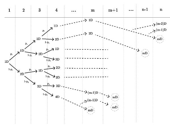
Figure 1: The probability tree for n-number of classifiers to have m-number of linearly independent votes. The numbers at the top of the figure represent the number of classifiers in the current system. D indicates dimension.

Discussion: This theorem numerically shows how adding a new classifier to the ensemble affects the probability of having an m-number of linearly independent votes. However, we want this probability to be as high as possible so that we are sure there are enough classifiers. For this reason, its limit should be known.

Theorem 3: If none of the $p_{k}$s is 1, then the probability of having m-number of linearly independent votes converges to 1 as n goes to infinity, i.e.

$$\lim_{n\to+\infty}(\prod_{i=1}^{m-1}(1-p_{i}))(\sum_{k=0}^{n-m}(\sum_{x_{1}+...+x_{m-1}=k}(\prod_{j=1}^{m-1}(p_{j}^{x_{j}})))=1$$ (3)

Proof: There are three possible cases for the above formula:
1) At least one of the $p_{k}$s is 1:
In this case the product $\prod_{i=1}^{m-1}(1-p_{i})$ evaluates to 0; hence the limit is 0.
2) All of the $p_{k}$s are 0.
In this case both $\sum_{k=0}^{n-m}(\sum_{x_{1}+...+x_{m-1}=k}(\prod_{j=1}^{m-1}(p_{j}^{x_{j}}))$ and $\prod_{i=1}^{m-1}(1-p_{i})$ evaluates to 1; hence the limit is 1.
3) None of the $p_{k}$ is 1, and at least one of them is not 0.
This case will be proven by induction.

Base case: For m = 2, the equation (2) is equal to

$$(1-p_{1})(1+p_{1}+p_{1}^{2}+p_{1}^{3}+...)$$

Since $0<p_{1}<1$,

$$1+p_{1}+p_{1}^{2}+p_{1}^{3}+...=\sum_{i=0}^{\infty}p_{1}=\frac{1}{1-p_{1}}$$

Hence,

$$(1-p_{1})(1+p_{1}+p_{1}^{2}+p_{1}^{3}+...)=1$$

Let the theorem hold for m = k+1, i.e.,

$$(1-p_{1})...(1-p_{k})(1+p_{1}+...+p_{k}+p_{1}^{2}+p_{1}p_{2}+...p_{k}^{2}+p_{1}^{3}+...)=1$$

$$\implies(1+p_{1}+...+p_{k}+p_{1}^{2}+p_{1}p_{2}+...p_{k}^{2}+p_{1}^{3}+...)=\frac{1}{(1-p_{1})...(1-p_{k})}$$

Then it is enough to show that

$$1+p_{1}+...+p_{k+1}+p_{1}^{2}+p_{1}p_{2}+...p_{k+1}^{2}+p_{1}^{3}+...=\frac{1}{(1-p_{1})...(1-p_{k+1})}$$

Let

$$1+p_{1}+...+p_{k+1}+p_{1}^{2}+p_{1}p_{2}+...p_{k+1}^{2}+p_{1}^{3}+...=A$$

Group the terms in the equation so that the terms with $p_{k+1}$ are gathered

$$1+p_{1}+...+p_{k}+p_{1}^{2}+p_{1}p_{2}+...p_{k}^{2}+p_{1}^{3}+...$$

$$+p_{k+1}+p_{k+1}p_{1}+...+p{k+1}^{2}+p_{k+1}p_{1}^{2}+...$$

$$=1+p_{1}+...+p_{k}+p_{1}^{2}+p_{1}p_{2}+...p_{k}^{2}+p_{1}^{3}+...$$

$$+p_{k+1}(1+p_{1}+...+p_{k+1}+p_{1}^{2}+p_{1}p_{2}+...p_{k+1}^{2}+p_{1}^{3}+...)$$

$$=\frac{1}{(1-p_{1})...(1-p_{k})}+p_{k+1}(A)=A$$

$$\implies A=\frac{1}{(1-p_{1})...(1-p_{k+1})}$$

Hence,

$$(1-p_{1})...(1-p_{k+1})(1+p_{1}+...+p_{k+1}+p_{1}^{2}+p_{1}p_{2}+...p_{k+1}^{2}+p_{1}^{3}+...)=1$$

Discussion: Theorem 2 showed how adding new classifiers affects the probability of having an m-number of linearly independent vectors. Theorem 3 shows that this probability converges to 1 when n gets larger and larger.

Table 2: Dataset Specifications. The first half is synthetic, the second half is real-life datasets. The calculated number of classifiers with the equation in Theorem 2 is given as Ideal #Classifiers

Dataset	#Inst.	#Attr.	#Class Labels	Ideal #Classifiers
RBF2	100,000	20	2	5
RBF4	100,000	20	4	11
RBF8	100,000	20	8	47
RBF16	100,000	20	8	274
Airlines	539,383	7	2	4
Elec	45,312	6	2	6
Rialto	82,250	27	10	31
Covtype	581,012	54	7	93

These three theorems explain the relationship between the number of component classifiers and ensemble performance. Furthermore, thinking backward for Theorem 2, we can set a target probability of having m-number of linearly independent votes, and calculate the minimum number of component classifiers n to reach that probability. This method provides us with a suggestion for the ensemble size.

4 Experiments

4.1 Setup

The experiments are conducted to investigate the relationship between the number of classifiers and the accuracy rate. Additionally, we calculate the minimum number of classifiers required using the equation in Theorem 2 with a target probability set at 0.999. For experiments, we use GOOWE (Geometrically Optimum and Online-Weighted Ensemble) as it already implements the geometric framework introduced [19]. Hoeffding Tree is used as the base classifier of GOOWE [20].

To evaluate the performance of the ensemble, we employ four real-world and four synthetic datasets. The synthetic datasets are created using the random RBF (Radial Basis Function) generator available in the scikit-multiflow library of Python. The specific details of the datasets are given in Table 2.

The probabilities $p_{k}$s (k=1,…,m-1) are experimentally calculated via Algorithm 1. We extend the GOOWE algorithm so that it also calculates these probabilities when iterating each vote.

Algorithm 1 Algorithm for Calculating p Values

1:$p\_array\leftarrow\text{zero array with length of \# class labels}$ // array that stores unsuccessful trials (vote is linearly // dependent) when adding new classifier vote to curMatrix.

2:$p\_total\leftarrow\text{zero array with length of \# class labels}$ // will be used to store total occurences of adding new // vote to curMatrix for calculating p values.

3:for each instance I in data stream do

4:     $voteMatrix\leftarrow\text{votes of component classifiers of ensemble for I }$

5:     $curMatrix\leftarrow\text{zero matrix with same dimensions as voteMatrix}$

6:     $prevDim\leftarrow 1$

7:     $curDim\leftarrow 1$

8:     for i in range(number of rows of voteMatrix) do // Add a row to curMatrix, and check the rank of it. // Update p_array and p_total accordingly.

9:         $curMatrix[i]\leftarrow voteMatrix[i]$

10:         if i == 0 then

11:              $continue$ // Since one vector is always linearly independent          

12:         $prevDim\leftarrow curDim$

13:         $curDim\leftarrow\text{rank of curMatrix}$

14:         if curDim == precDim then

15:              $p\_array[curDim-1]\leftarrow p\_array[curDim-1]+1$          

16:         $p\_total[prevDim-1]\leftarrow p\_total[prevDim-1]+1$

17:         if curDim == length of p_array then

18:              $break$               

19:for i in range(length of p_array) do // After this, p_array[i] = $p_{i+1}$

20:     if p_total[i] == 0 then

21:         $p\_array[i]\leftarrow 1$

22:     else

23:         $p\_array[i]\leftarrow p\_array[i]/p\_total[i]$      

4.2 Results

Table 2 summarizes the specifications of the datasets used in the experiments, including the ideal number of classifiers required for each dataset. Figure 2 is the plot of Accuracy Rate vs. Ensemble Size for different datasets.

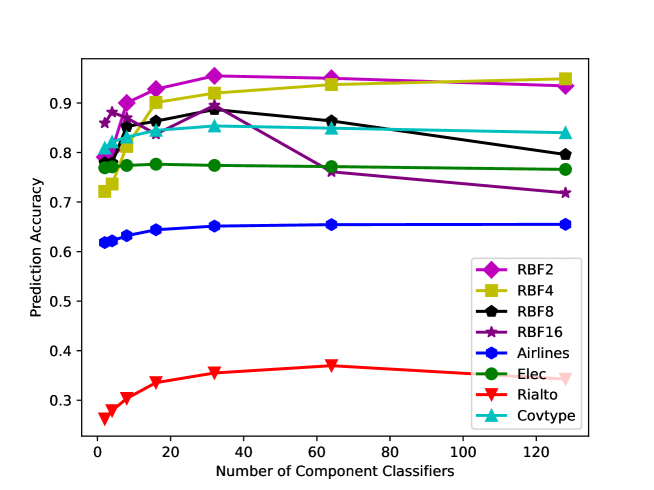
Figure 2: Prediction accuracy of the geometric framework with ensemble size ranging from 2 to 128. Synthetic datasets are named as RBF(number_of_class_labels).

We made several observations during our experiments. Firstly, Theorem 3 shows that equation (2) follows a convergent curve; the effect of adding more classifiers to the ensemble diminishes as the number of classifiers in the ensemble increases. This finding is in line with the rate of change of the accuracy rate, implying that beyond a certain point, adding more classifiers to the ensemble does not significantly improve performance.

Furthermore, we confirmed that as the number of classifiers of an ensemble increases, the accuracy rate generally improves. This observation aligns with the trend predicted by Formula (3): as the number of classifiers increases, the probability of obtaining a sufficient number of linearly independent votes approaches 1. However, for most of the datasets, the accuracy rate decreases after some point, especially for 128 component classifiers. This shows that there are factors affecting the ensemble performance other than the linear independency of component classifiers that we want to explore.

Moreover, for datasets with a low number of class labels, the calculated ideal ensemble size tends to be near the number of class labels. However, as the number of class labels increases, the ideal ensemble size deviates significantly from this linear relationship. This suggests that the complexity of achieving linearly independent votes among classifiers increases non-linearly with the number of class labels. Also, calculated ideal #classifiers match with empirical results only for the RBF8 dataset. This again shows the importance of factors other than the linear independence of component classifiers.

5 Conclusion & Future Work

In this paper, we show the importance of the linear dependence of classifiers for an ensemble. Using the probability of component classifiers being linear dependent, we provide a new perspective to understand how the number of classifiers in an ensemble affects the accuracy rate of that ensemble. Moreover, we provide a theoretical approach for determining ensemble size. The experiments we conducted show that, in general, the accuracy rate increases as the number of classifiers increases. This finding supports our theoretical framework.

We assumed that probabilities $p_{k}$s are the same for all classifiers in the ensemble, which means the classifiers are equally indistinguishable from each other. However, this is not true in real-life scenarios. In the future, we plan to investigate the individual classifier-level probability system to develop a more detailed theoretical framework.

References

- [1] Xibin Dong, Zhiwen Yu, Wenming Cao, Yifan Shi, and Qianli Ma. A survey on ensemble learning. Frontiers of Computer Science, 14:241–258, april 2020.
- [2] Bartosz Krawczyk, Leandro L. Minku, João Gama, Jerzy Stefanowski, and Michał Woźniak. Ensemble learning for data stream analysis: A survey. Information Fusion, 37:132–156, 2017.
- [3] Heitor Murilo Gomes, Jean Paul Barddal, Fabrício Enembreck, and Albert Bifet. A survey on ensemble learning for data stream classification. ACM Comput. Surv., 50:23:1–23:36, 03 2017.
- [4] Thomas G. Dietterich. Ensemble methods in machine learning. In Multiple Classifier Systems, pages 1–15, Berlin, Heidelberg, 2000. Springer Berlin Heidelberg.
- [5] Kamal Ali and Michael Pazzani. Error reduction through learning multiple descriptions. Machine Learning, 24, 11 1997.
- [6] Grigorios Tsoumakas, Ioannis Partalas, and I. Vlahavas. A taxonomy and short review of ensemble selection. ECAI 2008, Workshop on Supervised and Unsupervised Ensemble Methods and Their Applications, 01 2008.
- [7] Lior Rokach. Ensemble-based classifiers. Artif. Intell. Rev., 33:1–39, 02 2010.
- [8] Eric Bax. Selecting a number of voters for a voting ensemble. CoRR, abs/2104.11833, 2021.
- [9] Thais Oshiro, Pedro Perez, and José Baranauskas. How many trees in a random forest? volume 7376, 07 2012.
- [10] Patrice Latinne, Olivier Debeir, and Christine Decaestecker. Limiting the number of trees in random forests. volume 2096, pages 178–187, 07 2001.
- [11] Lena Pietruczuk, Leszek Rutkowski, Maciej Jaworski, and Piotr Duda. How to adjust an ensemble size in stream data mining? Information Sciences, 381:46–54, 2017.
- [12] Daniel Hernández-Lobato, Gonzalo Martínez-Muñoz, and Alberto Suárez. How large should ensembles of classifiers be? Pattern Recognition, 46(5):1323–1336, 2013.
- [13] Xiaohua Hu. Using rough sets theory and database operations to construct a good ensemble of classifiers for data mining applications. volume 233-240, pages 233–240, 01 2001.
- [14] Hamed Bonab and Fazli Can. Less is more: A comprehensive framework for the number of components of ensemble classifiers. IEEE Transactions on Neural Networks and Learning Systems, 30(9):2735–2745, 2019.
- [15] Shengli Wu and Fabio Crestani. A geometric framework for data fusion in information retrieval. Information Systems, 50:20–35, 2015.
- [16] Shengli Wu and Weimin Ding. A dataset-level geometric framework for ensemble classifiers. CoRR, abs/2106.08658, 2021.
- [17] Weimin Ding, Shengli Wu, and Chris Nugent. A multimodal fusion enabled ensemble approach for human activity recognition in smart homes. Health Informatics Journal, 29(2):14604582231171927, 2023. PMID: 37117157.
- [18] Hamed R. Bonab and Fazli Can. A theoretical framework on the ideal number of classifiers for online ensembles in data streams. In Proceedings of the 25th ACM International on Conference on Information and Knowledge Management, CIKM ’16, page 2053–2056, New York, NY, USA, 2016. Association for Computing Machinery.
- [19] Hamed R. Bonab and Fazli Can. Goowe: Geometrically optimum and online-weighted ensemble classifier for evolving data streams. ACM Trans. Knowl. Discov. Data, 12(2), Jan 2018.
- [20] Pedro Domingos and Geoff Hulten. Mining high-speed data streams. In Proceedings of the Sixth ACM SIGKDD International Conference on Knowledge Discovery and Data Mining, KDD ’00, page 71–80, New York, NY, USA, 2000. Association for Computing Machinery.