Hypergraph Structure Inference From Data
Under Smoothness Prior

Abstract

Hypergraphs are important for processing data with higher-order relationships involving more than two entities. In scenarios where explicit hypergraphs are not readily available, it is desirable to infer a meaningful hypergraph structure from the node features to capture the intrinsic relations within the data. However, existing methods either adopt simple pre-defined rules that fail to precisely capture the distribution of the potential hypergraph structure, or learn a mapping between hypergraph structures and node features but require a large amount of labelled data, i.e., pre-existing hypergraph structures, for training. Both restrict their applications in practical scenarios. To fill this gap, we propose a novel smoothness prior that enables us to design a method to infer the probability for each potential hyperedge without labelled data as supervision. The proposed prior indicates features of nodes in a hyperedge are highly correlated by the features of the hyperedge containing them. We use this prior to derive the relation between the hypergraph structure and the node features via probabilistic modelling. This allows us to develop an unsupervised inference method to estimate the probability for each potential hyperedge via solving an optimisation problem that has an analytical solution. Experiments on both synthetic and real-world data demonstrate that our method can learn meaningful hypergraph structures from data more efficiently than existing hypergraph structure inference methods.

1 Introduction

Hypergraphs, consisting of nodes and hyperedges, are a valuable generalisation of graphs. By allowing a hyperedge to connect an arbitrary number of nodes, a hypergraph can efficiently model the higher-order relationships involving more than two nodes [1]. There has been increasing attention to the usage of the hypergraph structure in many different research domains. For instance, hypergraph structures have been used to model the co-authorships in social science [2], to capture the spreading phenomena in epidemiology [3], and to improve the classification accuracy in machine learning [4]. However, not all real-world applications have readily available hypergraph structures, and $n$ given nodes can produce a total of $2^{n}$ different node combinations, with each combination corresponding to a potential hyperedge. A crucial task, in this case, is to infer a hypergraph structure from node data to capture the meaningful hidden higher-order relationships of the given entities. This is exactly the motivation of this paper.

In the literature, there are two main approaches to inferring a hypergraph structure from node features: rule-based and supervised-learning-based approaches. The rule-based approach [5, 6, 7, 8] constructs hypergraph structures based on heuristic rules. While it can yield topologies with some desirable properties (e.g., nodes in a hyperedge have similar features) without requiring any pre-existing hyperedges as supervision, these rules are often too simple to capture the underlying distribution of the ideal structure, lacking robustness and accuracy. Supervised-learning-based approaches [9, 10], on the other hand, use labelled data, namely, pre-existing hypergraph structures, as supervision to train neural networks to learn a mapping between node features and the hypergraph structures. Once the mapping is learned, the neural network can infer the probability of each potential hyperedge from node features. However, the reliance on extensive labelled data for training makes these methods only applicable to scenarios with vast amounts of pre-existing hypergraph structures.

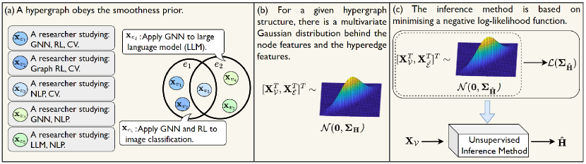
Figure 1: (a) A co-authorship hypergraph, where nodes are authors, hyperedges are papers, node features are authors’ research interests, and hyperedge features are topics of papers. Authors of the same paper tend to share similar research interests, which are also aligned with the topic of the paper written by them. (b) For a given hypergraph structure $\mathbf{H}$, there is a multivariate Gaussian distribution behind the node features $\mathbf{X}_{\mathcal{V}}$ and the hyperedge features $\mathbf{X}_{\mathcal{E}}$. Here, each $\mathbf{H}$ corresponds to a unique $\mathbf{\Sigma}_{\mathbf{H}}$. (c) The unsupervised inference method, which infers the potential hypergraph structure $\hat{\mathbf{H}}$ from $\mathbf{X}_{\mathcal{V}}$, is based on minimising the negative log-likelihood $\mathcal{L}(\mathbf{\Sigma}_{\hat{\mathbf{H}}})$. $\mathbf{X}_{\hat{\mathcal{E}}}$ denotes the features of potential hyperedges in $\hat{\mathbf{H}}$.

To address the above limitations, we propose a novel smoothness prior for hypergraph structure inference, which suggests that features of nodes in a hyperedge are highly correlated and this correlation results from their relation to the features of the hyperedge encompassing them; See Figure 1 (panel a) for the illustration of a hypergraph fitting this prior. Following this prior, we model the relation between a given hypergraph structure and the features of nodes on it via a multivariate Gaussian distribution whose covariance matrix is uniquely determined by the given hypergraph structure (Figure 1 (panel b)). Based on this probabilistic model, we develop a method to infer probabilities of potential hyperedges by solving an optimisation problem that only takes node features as input (Figure 1 (panel c)). The contributions of this work are summarised as follows:

$\bullet$ We propose a novel smoothness prior to describe the pattern behind node features on a hypergraph structure. Under this prior, we develop a probabilistic model that captures the relations between the hypergraph and the node data. The proposed smoothness prior and the probabilistic model provide a new perspective on the interactions between data and hypergraph structures.

$\bullet$ We design a novel unsupervised approach for hypergraph structure inference using the proposed smoothness prior. The key novelty of our approach is an inference method that directly learns the probability for each potential hyperedge by solving an optimisation problem that only requires node features as input.The unsupervised nature of our method means it can be applied to scenarios where pre-existing hypergraphs are difficult to obtain.

$\bullet$ We carry out experiments on both synthetic and real-world datasets to demonstrate that the proposed method significantly outperforms existing hypergraph structure inference methods. These results also showcase the efficacy of our smoothness prior in capturing the underlying pattern of real-world hypergraph data.

2 Preliminary

Hypergraphs. A hypergraph can be represented by a triplet $\mathcal{H}=\{\mathcal{V},\mathcal{E},\mathbf{H}\}$, where $\mathcal{V}=\{v_{1},v_{2},\cdots,v_{n}\}$ is the node set with $|\mathcal{V}|=n$, $\mathcal{E}=\{e_{1},e_{2},\cdots,e_{m}\}$ is the hyperedge set with $|\mathcal{E}|=m$, and $\mathbf{H}=[\operatorname{\textbf{h}}_{1},\operatorname{\textbf{h}}_{2},\cdots,\operatorname{\textbf{h}}_{m}]\in\{0,1\}^{n\times m}$ is a binary incidence matrix embedding a hypergraph structure in which $\operatorname{\textbf{h}}_{i}\in\{0,1\}^{n}$ represents the hyperedge $i$: $\mathbf{H}_{ji}=1$ indicates that hyperedge $i$ contains node $j$ and $\mathbf{H}_{ji}=0$ otherwise. The size of a hyperedge is the number of nodes contained in a hyperedge. If the size of a hyperedge is $k$, we call it a $k$-hyperedge.

Problem formulation. Let $\mathbf{X}_{\mathcal{V}}=[\mathbf{x}_{v_{1}},\mathbf{x}_{v_{2}},\cdots,\mathbf{x}_{v_{n}}]^{T}\in\mathbb{R}^{n\times d}$ denote the given node features, which is a matrix that contains $d$-dimensional features, and $\mathbf{H}\in\{0,1\}^{n\times m}$ be the ground-truth binary incidence matrix for the hypergraph structure associated with $\mathbf{X}_{\mathcal{V}}$. We assume $\mathbf{H}$ is drawn from a distribution that can be characterised by a weighted incidence matrix $\hat{\mathbf{H}}=[w_{1}\hat{\textbf{h}}_{1},w_{2}\hat{\textbf{h}}_{2},\cdots,w_{m_{p}}\hat{\textbf{h}}_{m_{p}}]\in\mathbb{R}^{n\times m_{p}}$, where $\hat{\textbf{h}}_{i}\in\{0,1\}^{n}$ is a potential hyperedge, $m_{p}$ is the number of potential hyperedges, and $w_{i}\in[0,1]$ defines the probability of the existence of $\hat{\textbf{h}}_{i}$ in $\mathbf{H}$. As $\hat{\textbf{h}}_{i}$ is pre-defined, we aim to infer a vector $\mathbf{w}=[w_{1},w_{2},\cdots,w_{m_{p}}]^{T}\in[0,1]^{m_{p}}$ that contains probabilities of all potential hyperedges, and we do so without training on known ground-truth hyperedges. After $\mathbf{w}$ is inferred, we construct $\mathbf{H}$ by $m$ most likely potential hyperedges. Without any constraints, $\hat{\mathbf{H}}$ would contain all the combinations of $n$ nodes as potential hyperedges and in this case $m_{p}=2^{n}$. In the absence of labelled data, a prior becomes essential to design an effective inference method that prioritises potential hyperedges capturing the desired higher-order interactions.

3 Methodology

In this section, we first propose a novel smoothness prior to describe the relation between the hypergraph and the node data (Section 3.1). This allows us to model the relation between a given hypergraph structure and the data observed on nodes via a multivariate Gaussian distribution whose covariance matrix is uniquely determined by the given structure (Section 3.2). Thereon, we develop an unsupervised inference method to estimate probabilities for potential hyperedges (Section 3.3).

3.1 Hypergraph Smoothness Prior

Motivation and definition. To infer hypergraph structures from node features without labelled data as supervision, we need to establish a prior that characterises the criteria by which nodes with certain features can be connected by a hyperedge. To do so, we propose a novel hypergraph smoothness prior: features of nodes in a hyperedge are highly correlated and this correlation results from their relation to the features of the hyperedge encompassing them. One interpretation of this assumption is that, if we treat each hyperedge as a virtual node whose features have the same dimension as the node features, then in a hyperedge nodes are assumed to be correlated with the corresponding virtual node.

Smoothness measure. Let $\mathbf{H}\in\{0,1\}^{n\times m}$ denote a given hypergraph structure, $\mathbf{X}_{\mathcal{V}}\in\mathbb{R}^{n\times d}$ be features of nodes on this structure, and $\mathbf{X}_{\mathcal{E}}=[\mathbf{x}_{e_{1}},\mathbf{x}_{e_{2}},\cdots,\mathbf{x}_{e_{m}}]^{T}\in\mathbb{R}^{m\times d}$ be features of corresponding hyperedges. Based on the proposed prior, for nodes with features smooth on a hypergraph, these nodes are close to each other and also to their corresponding hyperedges in the feature space. Hence, when $\mathbf{X}_{\mathcal{E}}$ is known, the smoothness of $\mathbf{X}_{\mathcal{V}}$ on $\mathbf{H}$ can be measured by:

$$f_{ev}(\mathbf{H},\mathbf{X}_{\mathcal{V}},\mathbf{X}_{\mathcal{E}})=\sum_{i=1}^{m}\sum_{v_{j}\in e_{i}}||\mathbf{x}_{e_{i}}-\mathbf{x}_{v_{j}}||^{2}_{2}=||\mathbf{s}_{\mathbf{H}}||_{1},$$ (1)

where $\mathbf{s}_{\mathbf{H}}=[s_{e_{1}},s_{e_{2}},\cdots,s_{e_{m}}]^{T}\in\mathbb{R}^{m}$, and $s_{e_{i}}=\sum_{v_{j}\in e_{i}}||\mathbf{x}_{e_{i}}-\mathbf{x}_{v_{j}}||^{2}_{2}$ measures the smoothness of node features in $e_{i}$. Therefore $f_{ev}(\mathbf{H},\mathbf{X}_{\mathcal{V}},\mathbf{X}_{\mathcal{E}})$ quantifies the smoothness of data on the hypergraph structure $\mathbf{H}$ by the sum of the squared $\ell_{2}$ distances between the node features and the corresponding hyperedge features: the smaller the $f_{ev}(\mathbf{H},\mathbf{X}_{\mathcal{V}},\mathbf{X}_{\mathcal{E}})$, the smoother the hypergraph is. In real-world scenarios, $\mathbf{X}_{\mathcal{E}}$ is usually implicit. Therefore, we further provide a function $f_{v}(\mathbf{H},\mathbf{X}_{\mathcal{V}})$ to approximate the hypergraph smoothness with only node features:

$$f_{v}(\mathbf{H},\mathbf{X}_{\mathcal{V}})=\sum_{i=1}^{m}\mathop{\max}\limits_{v_{j},v_{k}\in e_{i}}(||\mathbf{x}_{v_{j}}-\mathbf{x}_{v_{k}}||^{2}_{2})=||\mathbf{s}^{\prime}_{\mathbf{H}}||_{1},$$ (2)

where $\mathbf{s}^{\prime}_{\mathbf{H}}\!=\![s^{\prime}_{e_{1}},\!s^{\prime}_{e_{2}},\!\cdots,\!s^{\prime}_{e_{m}}]^{T}\in\mathbb{R}^{m}$, and $s^{\prime}_{e_{i}}\!=\!\mathop{\max}\limits_{v_{j},v_{k}\in e_{i}}(||\mathbf{x}_{v_{j}}-\mathbf{x}_{v_{k}}||_{2}^{2})$ is the largest squared $\ell_{2}$ distance between any pair of nodes in $e_{i}$. We prove that Eq. (2) is a lower bound for Eq. (1) as follows:

Theorem 1.

For any hypergraph structure $\mathbf{H}\in\{0,1\}^{n\times m}$, given node features $\mathbf{X}_{\mathcal{V}}=[\mathbf{x}_{v_{1}},\mathbf{x}_{v_{2}},\cdots,\mathbf{x}_{v_{n}}]^{T}\in\mathbb{R}^{n\times d}$, and hyperedge features $\mathbf{X}_{\mathcal{E}}=[\mathbf{x}_{e_{1}},\mathbf{x}_{e_{2}},\cdots,\mathbf{x}_{e_{m}}]^{T}\in\mathbb{R}^{m\times d}$, $f_{v}(\mathbf{H},\mathbf{X}_{\mathcal{V}})$ is a lower bound for $f_{ev}(\mathbf{H},\mathbf{X}_{\mathcal{V}},\mathbf{X}_{\mathcal{E}})$.

Proof.

To prove $f_{v}(\mathbf{H},\mathbf{X}_{\mathcal{V}})$ is a lower bound for $f_{ev}(\mathbf{H},\mathbf{X}_{\mathcal{V}},\mathbf{X}_{\mathcal{E}})$, it suffices to prove, for any hyperedge $e_{i}$ in $\mathbf{H}$, the following inequality holds:

$$\sum_{v_{j}\in e_{i}}||\mathbf{x}_{e_{i}}-\mathbf{x}_{v_{j}}||_{2}\geq\mathop{\max}\limits_{v_{j},v_{k}\in e_{i}}(||\mathbf{x}_{v_{j}}-\mathbf{x}_{v_{k}}||_{2}).$$ (3)

Without the loss of generality, in the feature space, let $v_{a}$ and $v_{b}$ be the two most distant nodes within $e_{i}$. By triangle inequality [11], we have:

$$\sum_{v_{j}\in e_{i}}||\mathbf{x}_{e_{i}}-\mathbf{x}_{v_{j}}||_{2}\geq||\mathbf{x}_{e_{i}}-\mathbf{x}_{v_{a}}||_{2}+||\mathbf{x}_{e_{i}}-\mathbf{x}_{v_{b}}||_{2}\geq||\mathbf{x}_{v_{a}}-\mathbf{x}_{v_{b}}||_{2}.$$

Hence, Eq. (3) holds, which proves the theorem. ∎

Notably, some previous works [12, 13, 14] also use Eq. (2) to measure the smoothness of data on a hypergraph. However, these works do not introduce the hyperedge features and use a different prior to define smoothness, which presumes the total variation of node features in a hyperedge is low.

3.2 Probabilistic Model

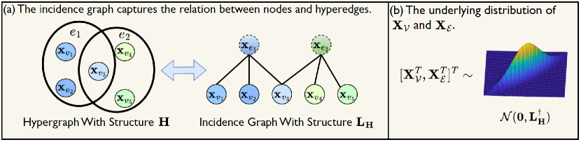
Figure 2: (a) A hypergraph $\mathbf{H}$, and its associated incidence graph with the graph Laplacian $\mathbf{L}_{\mathbf{H}}$. (b) With the incidence graph, $\mathbf{X}_{\mathcal{V}}$ and $\mathbf{X}_{\mathcal{E}}$ can be associated with a multivariate Gaussian distribution whose covariance matrix is the pseudoinverse of $\mathbf{L}_{\mathbf{H}}$.

In this section, under the proposed smoothness prior, we aim to relate a given hypergraph structure $\mathbf{H}$ to the node features $\mathbf{X}_{\mathcal{V}}$ by the distribution behind $\mathbf{X}_{\mathcal{V}}$ and $\mathbf{X}_{\mathcal{E}}$. To do so, we first model the relation between nodes and hyperedges by an incidence graph. Then, we derive a multivariate Gaussian distribution behind the features of nodes and hyperedges on the aforementioned incidence graph.

Incidence graph. A small quantity of the smoothness measure in Eq. (1) would indicate that, in the feature space, nodes are close to each other and also to their corresponding hyperedges. In this case, we capture the relation between nodes and hyperedges by using an incidence graph [15, 16, 17] corresponding to the hypergraph structure $\mathbf{H}$. Specifically, for the hypergraph $\mathcal{H}=\{\mathcal{V},\mathcal{E},\mathbf{H}\}$, we construct a unique incidence graph which is a bipartite graph $\mathcal{G}=\{\mathcal{V}\bigcup\mathcal{V}^{\prime},\mathcal{E}_{\mathcal{G}},\mathbf{L}_{\mathbf{H}}\}$, where $v_{i}\in\mathcal{V}$ is a node in $\mathcal{H}$, $v_{e_{j}}\in\mathcal{V}^{\prime}$ corresponds to the hyperedge $e_{j}$ in $\mathcal{H}$, and there is an edge between $v_{i}$ and $v_{e_{j}}$ if and only if $e_{j}$ contains $v_{i}$ in $\mathcal{H}$. The structure of $\mathcal{G}$ can be represented as a graph Laplacian matrix:

$$\small\mathbf{L}_{\mathbf{H}}=\begin{bmatrix}\operatorname{diag}(\mathbf{H}\textbf{1}_{m})&-\mathbf{H}\\ -\mathbf{H}^{T}&\operatorname{diag}(\mathbf{H}^{T}\textbf{1}_{n}),\end{bmatrix}$$ (4)

where $\mathbf{L}_{\mathbf{H}}\in\mathbb{R}^{(n+m)\times(n+m)}$, $\operatorname{diag}(\cdot)$ is a mapping that converts a vector into a diagonal matrix, and $\textbf{1}_{n}\in\{1\}^{n}$ and $\textbf{1}_{m}\in\{1\}^{m}$ are two all-one vectors. Further, the features of nodes in $\mathcal{V}$ are $\mathbf{X}_{\mathcal{V}}$, and the features of hyperedges in $\mathcal{V}^{\prime}$ are $\mathbf{X}_{\mathcal{E}}$. Figure 2 (panel a) shows an example of the incidence graph.

Underlying distribution of $\mathbf{X}_{\mathcal{V}}$ and $\mathbf{X}_{\mathcal{E}}$. We model the underlying distribution of $\mathbf{X}_{\mathcal{V}}$ and $\mathbf{X}_{\mathcal{E}}$ based on the incidence graph, following the literature of graph signal processing [18, 19, 20, 21]. Specifically, under the assumption of smoothness on a graph, the distribution of node features can be modelled by a multivariate Gaussian distribution whose covariance matrix is the pseudoinverse of the corresponding graph Laplacian matrix. In our incidence graph, nodes are connected to their corresponding hyperedges and by the smoothness prior in Section 3.1 they all have similar features. Therefore the underlying distribution of $\mathbf{X}_{\mathcal{V}}$ and $\mathbf{X}_{\mathcal{E}}$ can be modelled as:

$$\small[\mathbf{X}_{\mathcal{V}}^{T},\mathbf{X}_{\mathcal{E}}^{T}]^{T}\sim\mathcal{N}(\textbf{0},\mathbf{L}_{\mathbf{H}}^{\dagger}),$$ (5)

where $\mathbf{L}_{\mathbf{H}}^{\dagger}$ is the pseudoinverse of $\mathbf{L}_{\mathbf{H}}$. As $\mathbf{L}_{\mathbf{H}}$ is uniquely associated with $\mathbf{H}$, the relationship between $\mathbf{X}_{\mathcal{V}}$ and $\mathbf{H}$ is captured by Eq. (5). The probabilistic model is summarised in Figure 2 (panel b). In the following section, we use Eq. (5) as the foundation to design the inference framework.

3.3 Inference Framework

In this section, on the basis of the probabilistic model introduced in Section 3.2, our goal is to design an inference method that learns a vector $\mathbf{w}$ capable of capturing the probabilities for potential hyperedges, in which potential hyperedges that align more closely with the proposed smoothness prior are assigned higher probabilities. After the probabilities are learned by our method, we construct the target binary incidence matrix $\mathbf{H}$ by potential hyperedges with the top $m$ greatest probabilities.

Negative log-likelihood. Given the objective above, we first extend the probabilistic model in the previous section to the incidence matrix $\hat{\mathbf{H}}\in\mathbb{R}^{n\times m_{p}}$. Recall from Section 2 that $\hat{\mathbf{H}}$ is the weighted incidence matrix including all the potential hyperedges with their corresponding probabilities. According to Eq. (4), $\hat{\mathbf{H}}$ can be uniquely determined by the associated $\mathbf{L}_{\hat{\mathbf{H}}}$. Hence, we aim to develop an unsupervised method to infer $\hat{\mathbf{H}}$ from $\mathbf{X}_{\mathcal{V}}$ based on the negative log-likelihood of $\mathbf{L}_{\hat{\mathbf{H}}}$. Let $\mathbf{X}_{\hat{\mathcal{E}}}\in\mathbb{R}^{m_{p}\times d}$ denote features of the hyperedges in $\hat{\mathbf{H}}$, and $\mathbf{X}_{\hat{\mathbf{H}}}=[\mathbf{X}_{\mathcal{V}}^{T},\mathbf{X}_{\hat{\mathcal{E}}}^{T}]^{T}\in\mathbb{R}^{(n+m_{p})\times d}$. Then, according to the distribution described in Eq. (5), we have:

$$\small p(\mathbf{X}_{\hat{\mathbf{H}}}|\mathbf{L}_{\hat{\mathbf{H}}})\propto e^{-\mathbf{X}_{\hat{\mathbf{H}}}^{T}\mathbf{L}_{\hat{\mathbf{H}}}\mathbf{X}_{\hat{\mathbf{H}}}}.$$

Accordingly, the negative log-likelihood of $\mathbf{L}_{\hat{\mathbf{H}}}$ can be induced as:

$$\small\mathcal{L}(\mathbf{L}_{\hat{\mathbf{H}}}|\mathbf{X}_{\hat{\mathbf{H}}})\propto\mathbf{X}_{\hat{\mathbf{H}}}^{T}\mathbf{L}_{\hat{\mathbf{H}}}\mathbf{X}_{\hat{\mathbf{H}}}=\sum_{i=1}^{m_{p}}\sum_{v_{i}\in\hat{e}_{i}}w_{i}\leavevmode\nobreak\ ||\mathbf{x}_{\hat{e}_{i}}-\mathbf{x}_{v_{i}}||^{2}_{2},$$

where $w_{i}\in[0,1]$ is the probability of $\hat{e}_{i}$. Let us rewrite:

$$\small f_{wev}(\mathbf{w},\mathbf{X}_{\mathcal{V}},\mathbf{X}_{\hat{\mathcal{E}}})=\sum_{i=1}^{m_{p}}\sum_{v_{i}\in\hat{e}_{i}}w_{i}\leavevmode\nobreak\ ||\mathbf{x}_{\hat{e}_{i}}-\mathbf{x}_{v_{i}}||^{2}_{2}=\mathbf{w}^{T}\mathbf{s}_{\hat{\mathbf{H}}},$$ (6)

where $\mathbf{w}=[w_{1},w_{2},\cdots,w_{m_{p}}]^{T}\in[0,1]^{m_{p}}$, $\mathbf{s}_{\hat{\mathbf{H}}}=[s_{\hat{e}_{1}},s_{\hat{e}_{2}},\cdots,s_{\hat{e}_{m_{p}}}]^{T}\in\mathbb{R}^{m_{p}}$, and $s_{\hat{e}_{i}}=\sum_{v_{j}\in\hat{e}_{i}}||\mathbf{x}_{\hat{e}_{i}}-\mathbf{x}_{v_{j}}||^{2}_{2}$. Intuitively, Eq. (6) is a weighted version of the smoothness criterion defined in Eq. (1), which takes the probabilities as hyperedge weights. Accordingly, minimising $f_{wev}(\mathbf{w},\mathbf{X}_{\mathcal{V}},\mathbf{X}_{\hat{\mathcal{E}}})$ with respect to $\mathbf{w}$ can lead to a hypergraph structure that fits our smoothness prior.

There are two problems in directly using Eq. (6). Firstly, its computation requires $\mathbf{X}_{\hat{\mathcal{E}}}$, which is usually inaccessible in real-world scenarios. Secondly, minimising Eq. (6) in terms of $\mathbf{w}$, with the constrain $w_{i}\in[0,1]$, would result in a trivial solution where all the elements in $\mathbf{w}$ are zeros. Therefore, we work with an approximation of it:

$$\small f_{wv}(\mathbf{w},\mathbf{X}_{\mathcal{V}})=\mathbf{w}^{T}\mathbf{s}^{\prime}_{\hat{\mathbf{H}}}-\textbf{1}_{m_{p}}^{T}\log(\mathbf{w})+||\mathbf{w}||_{1},$$ (7)

where $\textbf{1}_{m_{p}}\in\{1\}^{m_{p}}$ is an all-one vector, $\mathbf{s}^{\prime}_{\mathbf{H}}=[s^{\prime}_{\hat{e}_{1}},s^{\prime}_{\hat{e}_{2}},\cdots,s^{\prime}_{\hat{e}_{m_{p}}}]^{T}\in\mathbb{R}^{m_{p}}$, and $s^{\prime}_{\hat{e}_{i}}=\mathop{\max}\limits_{v_{j},v_{k}\in\hat{e}_{i}}(||\mathbf{x}_{v_{j}}-\mathbf{x}_{v_{k}}||_{2}^{2})$. Here the first term is the weighted version of Eq. (2) and, as per Theorem 1, is a lower bound for $f_{wev}(\mathbf{w},\mathbf{X}_{\mathcal{V}},\mathbf{X}_{\hat{\mathcal{E}}})$. This term is used to promote the smoothness of node features on the learned hypergraph structure. The role of the second term in Eq. (7) serves to enforce the positivity of the learned probabilities, which can prevent $w_{i}$ from being zero and thereby avoid the creation of an empty hypergraph structure. The third term is used to ensure the sparsity of the target hypergraph structure, i.e., we would like only a small number of potential hyperedges to have significant probabilities.

Unsupervised inference method. On the basis of Eq. (7), essentially, inferring $\hat{\mathbf{H}}$ from $\mathbf{X}_{\mathcal{V}}$ is to infer $\mathbf{w}$ from $\mathbf{X}_{\mathcal{V}}$. Such an inference can be formulated as the following optimisation problem:

$$\small\mathop{\operatorname{min}}\limits_{\mathbf{w}}\leavevmode\nobreak\ \mathbf{w}^{T}\mathbf{s}^{\prime}_{\hat{\mathbf{H}}}-\textbf{1}_{m_{p}}^{T}\log(\mathbf{w})+||\mathbf{w}||_{1}\leavevmode\nobreak\ \leavevmode\nobreak\ \operatorname{s.t.}w_{i}\in(0,1].$$ (8)

To solve this problem, we take the derivative of the objective function with respect to each $w_{i}\in(0,1]$:

$$\small\frac{\partial f_{wv}}{\partial w_{i}}=s^{\prime}_{\hat{e}_{i}}-\frac{1}{w_{i}}+1,$$

and set it to zero:

$$\small w^{\star}_{i}=\frac{1}{s^{\prime}_{\hat{e}_{i}}+1},$$ (9)

$$\small\frac{\partial^{2}f_{wv}(w^{\star}_{i},\mathbf{X}_{\mathcal{V}})}{\partial^{2}w^{\star}_{i}}=\frac{1}{w^{\star^{2}}_{i}}>0,$$

hence, $\mathbf{w}^{\star}=[w^{\star}_{1},w^{\star}_{2},\cdots,w^{\star}_{m_{p}}]^{T}\in(0,1]^{m_{p}}$ is the analytical solution for Eq. (8) under the constraints each $w_{i}\in(0,1]$. In practice, we use Eq. (9) to infer the probabilities for potential hyperedges. Solving Eq. (8) does not require labelled data, so the proposed inference method is completely unsupervised.

Hypergraph structure construction. Notably, without any constraints, $m_{p}=2^{n}$ which makes solving Eq. (8) extremely time-consuming. Moreover, based on (9), the inferred probability of $\hat{e}_{i}$ is inversely proportional to the maximum distance between the two nodes in it, which indicates that a hyperedge is more likely to be formed by nodes that are close to each other in the feature space. Hence, we propose to constrain the set of potential hyperedges in $\hat{\mathbf{H}}$ in a way similar to that in [18]:for a given set $\mathcal{K}_{L}=\{k_{1},k_{2},\cdots,k_{L}\}$ that collects $L$ desired hyperedge sizes, each potential $k_{l}$-hyperedge is formed by a node with its $k_{l}-1$ nearest neighbours in the feature space. By doing so, we constrain the number of potential hyperedges always not greater than $Ln$, and ensure that all the potential hyperedges consist of nodes with similar features. We then use this constrained set to compute $s^{\prime}_{\hat{e}_{i}}$ and solve Eq. (8) based on Eq. (9). Once $\mathbf{w}^{\star}$ is obtained, we construct $\mathbf{H}$ with the $m$ most likely hyperedges. The overall approach is summarised in Algortithm 1.

0:  Node features $\mathbf{X}_{\mathcal{V}}$, a set of hyperedge sizes $\mathcal{K}_{L}$, and the number of the target hyperedges $m$.

0:  Binary incidence matrix $\mathbf{H}$.

1:  For each hyperedge size $k_{l}$, introduce potential $k_{l}$-hyperedges to $\hat{\mathbf{H}}$, which are formed by nodes with their $k_{l}-1$ nearest neighbours in the feature space.

2:  Compute $\mathbf{s}^{\prime}_{\hat{\mathbf{H}}}$ by $\mathbf{X}_{\mathcal{V}}$ for the selected potential hyperedges in $\hat{\mathbf{H}}$.

3:  Use $\mathbf{s}^{\prime}_{\hat{\mathbf{H}}}$ to generate $\mathbf{w}^{\star}$ based on Eq. (9).

4:  Form $\mathbf{H}$ based on the generated probabilities $\mathbf{w}^{\star}$.

Algorithm 1 Hypergraph Structure Inference Under Smoothness Prior (HGSI)

4 Related Works

Learning with pre-existing hypergraphs.

There exists a body of works for analysing data residing on a pre-existing hypergraph structure. Many of them [4, 22, 23] extend the message-passing paradigm in graph machine learning [24] to develop hypergraph neural networks using a two-stage message-passing paradigm to learn node features for specific downstream tasks, e.g., node classification, with given hypergraph structures. Our work is notably different as we do not assume the knowledge of a pre-existing hypergraph structure and, in fact, aim at inferring it from observed node data. Recently, a few works [5, 12, 25] assume that the pre-defined hypergraph structures might be perturbed or contain information irrelevant to the downstream task, hence propose to optimise the node features and hypergraph structures simultaneously for specific downstream tasks. There are two key distinctions between these works and ours. First, they begin with node features and pre-defined hypergraph structures, i.e., incidence matrices or high-dimensional tensors. On the contrary, we use node features to learn hypergraph structures from scratch. Second, their focus is on downstream task performance, while we have no downstream tasks and solely aim at inferring the hypergraph structure.

Hypergraph structure inference.

Existing hypergraph structure inference approaches can be divided into two categories: rule-based and supervised-learning-based approaches. The rule-based approach either assumes that in an hyperedge nodes have similar features, or that a hyperedge can be decomposed as a set of pairwise edges. The methods built upon the first assumption usually construct a hypergraph by setting hyperedges as clusters determined by the $k$-means algorithm [5, 6, 7]. Approaches under the second assumption typically create a hypergraph with specific connected components, e.g., cliques or communities, in a graph structure [8, 26]. These rule-based methods can provide hypergraph structures with some desirable properties, but they fail to disclose the distribution behind the generated hypergraph structure, which limits their robustness and inference accuracy. On the other hand, recent works [9, 10] use ground-truth hypergraph structures associated with node features to train a neural network that learns a mapping between node features and ground-truth structures. After the mapping is learned, the neural network can estimate the probabilities of hyperedges and form a hypergraph structure accordingly. However, these supervised-learning-based approaches often require a significant amount of ground-truth hyperedges and associated node features for reliable training, hence limiting their application in scenarios where labelled data are scarce. We address the limitations of both categories in this paper. First, we propose a novel smoothness prior for hypergraph structure inference. With this prior, we capture the relation between the hypergraph and the node data via a probabilistic model. Second, leveraging the proposed prior, we design an unsupervised hypergraph structure inference method that can estimate the probability for each potential hyperedge without training on labelled data.

5 Experiments

5.1 Experiment setup

Datasets. In the synthetic dataset, a hypergraph with node features is generated in two steps: 1) generate the ground-truth hypergraph structures based on the algorithm in [27]; 2) use the generated structures to get node features by $[\mathbf{X}_{\mathcal{V}}^{T},\mathbf{X}_{\mathcal{E}}^{T}]^{T}\sim\mathcal{N}(\textbf{0},(\mathbf{L}_{\mathbf{H}}+\sigma^{2}\textbf{I})^{-1})$ , where we set the dimension of the node features as 1000, and $\sigma$ is a small positive constant which is set as $10^{-3}$ in our experiments. Although we have the features of hyperedges in the synthetic dataset, these features are not used in our inference approach. The real-world dataset involves three real-world hypergraphs: Cora, DBLP, and Yelp, which are obtained from the pre-processed data in [4]. Cora and DBLP are two co-authorship hypergraphs, where nodes are authors, a hyperedge containing authors of a specific paper, and the node features are formulated by the bag-of-words model with keywords related to the authors’ research interests. Yelp is a customership hypergraph, where a node is a customer, a hyperedge including customers of a specific restaurant, and node features are formulated by the bag-of-words model with keywords describing the dining preferences of each customer. Cora contains 479 nodes each with a feature dimension of 1433 and 220 hyperedges whose sizes are 3 or 8. DBLP has 626 nodes each with a feature dimension of 1425 and 212 hyperedges whose sizes are 4. Yelp includes 688 nodes each with a feature dimension of 1860 and 120 hyperedges whose sizes are 6. Notably, on the real-world datasets, we assume that we can only get access to the number of the overall target hyperedges, which is denoted as $K$, and we take the hyperedges with top $K$ probabilities to form the generated incidence matrix. On the synthetic datasets, we assume that we can obtain the number of hyperedges belonging to different sizes. With this knowledge, we proceed by ranking and selecting the hyperedges within each size category.

Baselines. We choose GroupNet [6], HGSL [8], and NEO [28] as our baselines. These are unsupervised rule-based approaches. GroupNet assumes that each node contributes to at least one hyperedge whose internal nodes are highly correlated in terms of cosine similarity. HGSL learn the hypergraph structure from node features by doing community detection on a learnable line graph. NEO is an overlapping k-means algorithm, in which generated clusters are set as hyperedges in the hypergraph.

Metrics. We compare the proposed approach with its variation and baselines in finding the binary incidence matrix embedding the ground-truth hyperedges. We use F1-score and the normalised mean squared error for hypergraph recovery (HGMSE) to measure the performance of these methods. The higher the F1 score, the more accurate the binary incidence matrix is generated by the method. The smaller the HGMSE, the closer the generated binary incidence matrix and ground-truth incidence matrix are. In the following, we show the results of the average F1-Score/HGMSE and the associated std in 10 runs. Note that the performances of NEO and HGSL vary according to different random seeds, because NEO needs to randomly initialize the cluster centres and HGSL needs to do random selection in its community detection step. The inference processes of GroupNet and HGSI are deterministic, so their performances do not vary according to random seeds.

Table 1: F1-Score of methods on synthetic datasets with different numbers of hyperedge sizes and overlapping rates.

Models / Datasets	Overlap Rate10%		Overlap Rate 30%		Overlap Rate 50%
	UniHG	MultiHG	UniHG	MultiHG	UniHG	MultiHG
GroupNet [6]	0.8676	0.2166	0.6059	0.1985	0.5260	0.1935
HGSL [8]	0.9173 $\pm$ 0.0024	0.8144 $\pm$ 0.0000	0.4754 $\pm$ 0.0044	0.4494 $\pm$ 0.0024	0.2335 $\pm$ 0.0018	0.1883 $\pm$ 0.0028
NEO [28]	0.9063 $\pm$ 0.0482	0.8666 $\pm$ 0.0142	0.4631 $\pm$ 0.0220	0.4105 $\pm$ 0.0132	0.1578 $\pm$ 0.0155	0.1425 $\pm$ 0.0094
HGSI	1.0000	1.0000	0.9301	0.9112	0.9049	0.8984

Table 2: HGMSE of methods on synthetic datasets with different numbers of hyperedge sizes and overlapping rates.

Models / Datasets	Overlap Rate10%		Overlap Rate 30%		Overlap Rate 50%
	UniHG	MultiHG	UniHG	MultiHG	UniHG	MultiHG
GroupNet [6]	0.1376	0.5711	0.1815	0.6047	0.3118	0.6218
HGSL [8]	0.0146 $\pm$ 0.0007	0.0306 $\pm$ 0.0000	0.1231 $\pm$ 0.0018	0.1891 $\pm$ 0.0015	0.7357 $\pm$ 0.0004	0.6341 $\pm$ 0.0007
NEO [28]	0.0445 $\pm$ 0.0004	0.0406 $\pm$ 0.0024	0.6504 $\pm$ 0.0872	0.8826 $\pm$ 0.0336	1.0691 $\pm$ 0.0634	2.1412 $\pm$ 0.0413
HGSI	0.0000	0.0000	0.0155	0.0193	0.0230	0.0277

5.2 Synthetic Dataset

In this section, we evaluate the proposed method from two perspectives. Firstly, we present that the proposed method can learn ground-truth hypergraph structures with varying properties from data fitting the hypergraph smoothness prior. Secondly, we show that the smoothness criterion formulated as Eq. (2) plays a key role in our method. Regarding the first perspective, our experiments focus on four key structural metrics: the number of nodes, the hyperedge size, the overlap rate, and the number of hyperedge sizes. The overlap rate of a hyperedge is defined as the ratio of nodes in the hyperedge that are involved in more than one hyperedge to the total number of nodes. The average overlapping rate of a hypergraph is the mean of its hyperedges’ overlapping rates [8]. For instance, the overlap rate of the hypergraph structure shown in Figure 2 is around 33.3%. For the second perspective, we conduct an ablation study on the smoothness criterion used in our method. Each result here is the average F1-score and HGMSE computed on 32 different hypergraphs.

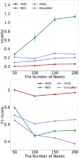
(a) Impacted by the number of nodes.

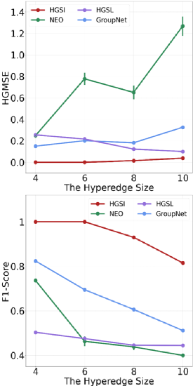
(b) Impacted by the hyperedge size.

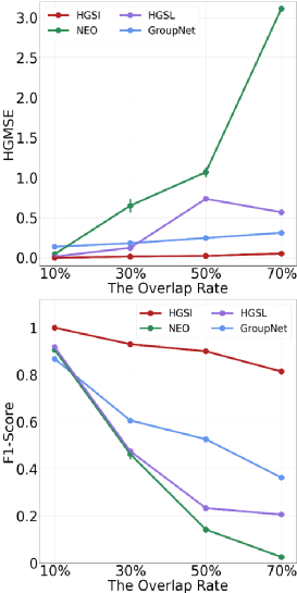
(c) Impacted by the overlap rate.

Figure 3: The impacts brought by the properties of the ground-truth hypergraph structure.

Table 3: F1-Score, Precision and Recall of GroupNet on UniHG and MultiHG with different overlapping rates.

	Overlap Rate10%			Overlap Rate 30%			Overlap Rate 50%
	F1-Score	Precision	Recall	F1-Score	Precision	Recall	F1-Score	Precision	Recall
UniHG	0.8676	0.7662	1.0000	0.6059	0.4360	0.9928	0.5260	0.3588	0.9853
MultiHG	0.2166	0.1212	1.0000	0.1985	0.1102	0.9953	0.1935	0.1074	0.9732

Table 4: F1-score of different methods in inferring real-world hypergraph structures.

Models / Datasets	Cora	DBLP	Yelp
GroupNet [6]	0.5310	0.8849	0.8898
HGSL [8]	0.4297 $\pm$ 0.0001	0.4698 $\pm$ 0.0000	0.7215 $\pm$ 0.0010
NEO [28]	0.4338 $\pm$ 0.0138	0.4474 $\pm$ 0.0103	0.7283 $\pm$ 0.0085
HGSI	0.8909	0.9151	0.9250

Table 5: HGMSE of different methods in inferring real-world hypergraph structures.

Models / Datasets	Cora	DBLP	Yelp
GroupNet [6]	0.4015	0.0758	0.0771
HGSL [8]	0.2001 $\pm$ 0.0001	0.0895 $\pm$ 0.0000	0.1401$\pm$ 0.0000
NEO [28]	0.6069 $\pm$ 0.0206	0.4431 $\pm$ 0.0164	0.0915 $\pm$ 0.0140
HGSI	0.0947	0.0425	0.0333

Figure 4: The proposed smoothness criterion enables HGSI to achieve optimal performance on synthetic data.

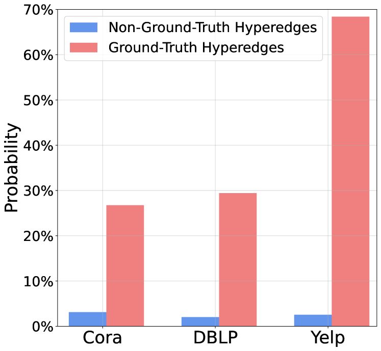
Figure 5: The red/blue bar represents the average probabilities generated by HGSI for the ground-truth/non-ground-truth potential hyperedges in the potential hypergraph structure.

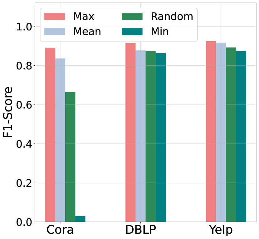
Figure 6: The proposed smoothness criterion enables HGSI to achieve optimal performance on real-world data.

The number of nodes. Figure 3(a) shows the impact of the number of nodes in the ground-truth hypergraphs. Here we let all hyperedges in a hypergraph be 8-hyperedges and fix the overlap rate of each hypergraph as 30%. The increase in the number of nodes would cause an increase in the search space of the tested methods. According to the structure construction constraint proposed in Section 3.3, the search space of our methods grows linearly with the number of nodes. Therefore, HGSI is hardly influenced by the increase in the number of nodes.

The hyperedge size. Figure 3(b) exhibits the impact brought by the size of hyperedges in the ground-truth hypergraphs. Here we fix the number of nodes, the overlap rate, and the number of hyperedge sizes of each hypergraph as 100, 30%, and 1 respectively. The growing sizes of hyperedges necessitate inference techniques that incorporate a more significant number of node features to identify relevant hyperedges, resulting in heightened inference complexity. Thus, the F1-Score for all employed methods declines as the hypergraph size within the ground-truth structure expands.

The overlap rate. Figure 3(c) displays the impact from the overlap rate in the ground-truth hypergraphs. Here we fix the number of nodes of each hypergraph as 100 and let all hyperedges in a hypergraph be 8-hyperedges. The escalating overlap rate in ground-truth hypergraphs can make nodes in different hyperedges have similar features, thus leading to a blurring of the boundaries between different hyperedges. Therefore, this exacerbates the challenges encountered during the inference process. Accordingly, the performances of all the methods drop when the overlap rate increases.

The number of hyperedge sizes. Table 1 and Table 2 show the impact brought by the number of hyperedge sizes under different overlap rates. Here each hypergraph consists of 100 nodes. Moreover, UniHG denotes hypergraphs containing hyperedges in only size 8, and MultiHG represents hypergraphs including hyperedges in three different sizes: 7, 8, and 9. We note that this metric mainly influences the performance of GroupNet. This is because the number of hyperedges in its output increases significantly when the number of hyperedge sizes grows, which results in a substantial decrease in its precision. Additional results for the recall and precision of GroupNet are in Table 3.

Remark. Regardless of the properties of the ground-truth hypergraph structures, HGSI generates the most accurate structure compared to other methods, which confirms the accuracy and robustness of the proposed approach. We attribute these promising outcomes to two factors. Firstly, solving the optimisation problem in Eq. (9) can result in accurate probabilities for potential hyperedges. Secondly, the ground-truth hyperedges can be precisely captured in the potential hyperedge structure by the proposed structure construction constraint, which helps HGSI to reduce the search space efficiently.

Ablation study on the smoothness criterion. We empirically study how the smoothness criterion formulated as Eq. (2) influences HGSI. We denote the proposed smoothness criterion as Max and compare it with three other smoothness criteria: Mean, Random and Min. Mean calculates smoothness based on the average squared $\ell_{2}$ distance between nodes in a hyperedge, Random uses the squared $\ell_{2}$ distance of a random node pair, and Min considers the smallest squared $\ell_{2}$ distance between nodes in the hyperedge. We experiment on a 200-node dataset with hyperedges of size 8 and a 30% overlap rate. The results are summarized as Figure 6, which show that the proposed smoothness criterion enables HGSI to achieve its optimal performance. These results confirm that the smoothness criterion formulated as Eq. (2) plays a critical role in HGSI. Figure 6 summarizes the results, demonstrating that the proposed smoothness criterion optimizes HGSI performance. These findings confirm the crucial role of the proposed smoothness criterion in HGSI.

5.3 Real-World Dataset

Results. The performance of each method in inferring the real-world hypergraph structures from node features is presented in Table 5 and Table 5. These results show that the proposed HGSI achieve state-of-the-art performance in inferring every real-world hypergraph structure with respect to both F1-Score and HGMSE. Furthermore, Figure 6 visualises the probabilities generated by HGSI for the ground-truth and non-ground-truth hyperedges in the potential hypergraph structure. These figures illustrate that, for every real-world hypergraph, HGSI generates much higher probabilities for ground-truth hyperedges compared to non-ground-truth hyperedges in the potential hypergraph structure. Both the quantitative results and the visualisation reflect that the proposed inference method can use the given node features to generate reliable probabilities for potential hyperedges in the real world. Additionally, the proposed hypergraph smoothness prior demonstrates the ability to capture the relationship between the real-world hypergraph structure and the node features associated with it.

Ablation study on the smoothness criterion. We empirically test the proposed smoothness criterion on real-world datasets. Figure 6 illustrates that on all of the chosen real-world datasets, the smoothness formulated as Eq. (2) makes HGSI achieve the best performance, thereby confirming that the proposed smoothness criterion plays a crucial role in capturing the real-world hypergraph-data relation.

6 Discussions on Limitations

We discuss the limitations from two main perspectives: the formulation of our problem, and the design of our methodology.

In this paper, we specifically focus on undirected and static hypergraphs and do not explore the inference of directed and dynamic hypergraphs. Generalising the proposed smoothness prior to inferring directed and dynamic hypergraphs poses significant challenges. A fixed symmetric matrix, e.g., a covariance matrix, might not adequately capture the hypergraph-data relationship in the context of directed and dynamic hypergraphs. Therefore, we need to find a new mathematical framework to model the relation between node features and the corresponding directed and dynamic hypergraph structures. We leave this non-trivial generalisation of the proposed smoothness prior to future work.

For the design of our methodology, there are three limitations that should be acknowledged. Firstly, our approach relies on a fixed smoothness prior. Although our main paper demonstrates that this prior is effective in learning hypergraphs where nodes within a hyperedge share correlated features, real-world data exhibits significant variations across different domains. There may be cases where nodes in a hyperedge have uncorrelated features. In such cases, our method may not yield meaningful hypergraph structures. To address this limitation, we plan to develop a few-shot learning-based model that leverages supervision to produce meaningful hypergraph structures across various application domains in future. Secondly, to ensure computational efficiency, the proposed approach focuses on estimating probabilities for hyperedges that satisfy the specific constraint proposed in our paper. This constraint presumes that for a given set $\mathcal{K}_{L}=\{k_{1},k_{2},\cdots,k_{L}\}$ that collects $L$ desired hyperedge sizes, each potential $k_{l}$-hyperedge is formed by a node with its $k_{l}-1$ nearest neighbours in the feature space. The experimental results display that, with this constraint, our method outperforms previous hypergraph inference methods. However, we acknowledge that there may exist alternative constraints or approaches to efficiently estimate probabilities for all $2^{n}$ potential hyperedges formed by $n$ given nodes, which could potentially lead to improved performance. We set the exploration of this direction to future research based on the smoothness prior proposed in this paper. Finally, for obtaining a binary incidence matrix, we require the number of target hyperedges. One way to approximate the number of target hyperedges is to use the number of potential hyperedges fitting the proposed constraint:

$$\small m^{a}=\sum_{i=1}^{L}m_{k_{i}}^{p}\rho_{k_{i}},$$

where $m^{a}$ is the approximated number of overall potential hyperedges, $m_{k_{i}}^{p}$ is the number of the potential $k_{i}$-hyperedges fitting the proposed constraint, and $\rho_{k_{i}}\in[0,1]$ is a hyperparameter. In order to design a more automatic unsupervised method to approximate the number of target hyperedges, further empirical studies are required to identify the underlying distribution of the number of hyperedges in real-world data. We leave it as future work built upon the inference approach proposed in this paper.

7 Conclusion

We propose a novel smoothness prior for the hypergraph structure inference, which tells that features of nodes in a hyperedge are highly correlated and this correlation results from the features of the hyperedge encompassing them. Under this prior, we design an original unsupervised hypergraph structure inference approach. Extensive experiments on both synthetic and real-world datasets not only confirm the efficiency of the proposed approach in inferring hypergraph structures from observed node features but also reveal the potential of the proposed prior in capturing the real-world hypergraph-data relation. We believe both the proposed prior and the proposed inference approach can benefit the hypergraph machine learning community through the inference of an appropriate hypergraph structure to capture the higher-order relationships among data.

References

- [1] C. Bick, E. Gross, H. A. Harrington, and M. T. Schaub, “What are higher-order networks?” arXiv preprint arXiv:2104.11329, 2021.
- [2] Y. Han, B. Zhou, J. Pei, and Y. Jia, “Understanding importance of collaborations in co-authorship networks: A supportiveness analysis approach,” in Proceedings of the 2009 SIAM International Conference on Data Mining. SIAM, 2009, pp. 1112–1123.
- [3] B. Jhun, “Effective epidemic containment strategy in hypergraphs,” Physical Review Research, vol. 3, no. 3, p. 033282, 2021.
- [4] E. Chien, C. Pan, J. Peng, and O. Milenkovic, “You are allset: A multiset function framework for hypergraph neural networks,” in International Conference on Learning Representations, 2022. [Online]. Available: https://openreview.net/forum?id=hpBTIv2uy_E
- [5] Y. Gao, Z. Zhang, H. Lin, X. Zhao, S. Du, and C. Zou, “Hypergraph learning: Methods and practices,” IEEE Transactions on Pattern Analysis and Machine Intelligence, vol. 44, no. 5, pp. 2548–2566, 2020.
- [6] C. Xu, M. Li, Z. Ni, Y. Zhang, and S. Chen, “Groupnet: Multiscale hypergraph neural networks for trajectory prediction with relational reasoning,” in The IEEE/CVF Conference on Computer Vision and Pattern Recognition (CVPR), 2022.
- [7] C. Xu, Y. Wei, B. Tang, S. Yin, Y. Zhang, and S. Chen, “Dynamic-group-aware networks for multi-agent trajectory prediction with relational reasoning,” arXiv preprint arXiv:2206.13114, 2022.
- [8] B. Tang, S. Chen, and X. Dong, “Learning hypergraphs from signals with dual smoothness prior,” in ICASSP 2023-2023 IEEE International Conference on Acoustics, Speech and Signal Processing (ICASSP). IEEE, 2023, pp. 1–5.
- [9] H. Serviansky, N. Segol, J. Shlomi, K. Cranmer, E. Gross, H. Maron, and Y. Lipman, “Set2graph: Learning graphs from sets,” Advances in Neural Information Processing Systems, vol. 33, pp. 22 080–22 091, 2020.
- [10] D. W. Zhang, G. J. Burghouts, and C. G. Snoek, “Pruning edges and gradients to learn hypergraphs from larger sets,” in Learning on Graphs Conference. PMLR, 2022, pp. 53–1.
- [11] M. Abramowitz, I. A. Stegun, and R. H. Romer, “Handbook of mathematical functions with formulas, graphs, and mathematical tables,” 1988.
- [12] C. H. Nguyen and H. Mamitsuka, “Learning on hypergraphs with sparsity,” IEEE Transactions on Pattern Analysis and Machine Intelligence, vol. 43, no. 8, pp. 2710–2722, 2021.
- [13] M. Hein, S. Setzer, L. Jost, and S. S. Rangapuram, “The total variation on hypergraphs-learning on hypergraphs revisited,” Advances in Neural Information Processing Systems, vol. 26, 2013.
- [14] R. Qu, H. Feng, C. Xu, and B. Hu, “Analysis of hypergraph signals via high-order total variation,” Symmetry, vol. 14, no. 3, p. 543, 2022.
- [15] C. Godsil and G. F. Royle, Algebraic graph theory. Springer Science & Business Media, 2001, vol. 207.
- [16] M. A. Bahmanian and M. Sajna, “Connection and separation in hypergraphs,” Theory and Applications of Graphs, vol. 2, no. 2, p. 5, 2015.
- [17] X. Ouvrard, “Hypergraphs: an introduction and review,” arXiv preprint arXiv:2002.05014, 2020.
- [18] V. Kalofolias and N. Perraudin, “Large scale graph learning from smooth signals,” arXiv preprint arXiv:1710.05654, 2017.
- [19] X. Dong, D. Thanou, P. Frossard, and P. Vandergheynst, “Learning laplacian matrix in smooth graph signal representations,” IEEE Transactions on Signal Processing, vol. 64, no. 23, pp. 6160–6173, 2016.
- [20] S. P. Chepuri, S. Liu, G. Leus, and A. O. Hero, “Learning sparse graphs under smoothness prior,” in 2017 IEEE International Conference on Acoustics, Speech and Signal Processing (ICASSP). IEEE, 2017, pp. 6508–6512.
- [21] X. Pu, T. Cao, X. Zhang, X. Dong, and S. Chen, “Learning to learn graph topologies,” Advances in Neural Information Processing Systems, vol. 34, pp. 4249–4262, 2021.
- [22] Y. Feng, H. You, Z. Zhang, R. Ji, and Y. Gao, “Hypergraph neural networks,” in Proceedings of the AAAI conference on artificial intelligence, vol. 33, no. 01, 2019, pp. 3558–3565.
- [23] J. Huang and J. Yang, “Unignn: a unified framework for graph and hypergraph neural networks,” in Proceedings of the Thirtieth International Joint Conference on Artificial Intelligence, IJCAI-21, 2021.
- [24] J. Zhou, G. Cui, S. Hu, Z. Zhang, C. Yang, Z. Liu, L. Wang, C. Li, and M. Sun, “Graph neural networks: A review of methods and applications,” AI open, vol. 1, pp. 57–81, 2020.
- [25] D. Cai, M. Song, C. Sun, B. Zhang, S. Hong, and H. Li, “Hypergraph structure learning for hypergraph neural networks,” in Proceedings of the Thirty-First International Joint Conference on Artificial Intelligence, IJCAI-22, L. D. Raedt, Ed. International Joint Conferences on Artificial Intelligence Organization, 7 2022, pp. 1923–1929, main Track. [Online]. Available: https://doi.org/10.24963/ijcai.2022/267
- [26] J.-G. Young, G. Petri, and T. P. Peixoto, “Hypergraph reconstruction from network data,” Communications Physics, vol. 4, pp. 1–11, 2021.
- [27] M. T. Do, S.-e. Yoon, B. Hooi, and K. Shin, “Structural patterns and generative models of real-world hypergraphs,” in ACM SIGKDD International Conference on Knowledge Discovery and Data Mining, 2020.
- [28] J. J. Whang, Y. Hou, D. F. Gleich, and I. S. Dhillon, “Non-exhaustive, overlapping clustering,” IEEE Transactions on Pattern Analysis and Machine Intelligence, vol. 41, no. 11, pp. 2644–2659, 2019.