Magnetostatic modes and criticality in uniaxial magnetic materials

Abstract

We analyze modes in a dipole-dipole coupled quantum magnetic material, taking into consideration domain structure and other shape effects present in any real magnet. We find that the soft mode governing quantum criticality in a non-ellipsoidal sample is an inhomogeneous magnetostatic mode which negates dynamic, demagnetization-field effects. The demagnetization field is analyzed from a microscopic perspective. Furthermore, we find a magnetostatic mode originating from variations in the magnetization of the sample, caused by domain structure and quantum or thermal fluctuations, will be lower in energy than the soft mode governing quantum criticality in the bulk of the magnet. Experimental evidence for these theoretical results is provided by analysis of electronuclear modes in LiHoF₄, an archetypal dipolar quantum Ising material, in a microwave resonator.

I Introduction

The transverse-field Ising model (TFIM) exhibits a quantum phase transition between an ordered ferromagnetic phase, and a paramagnetic phase, as one tunes the applied transverse field [1, 2, 3]. Assuming a needle shaped sample for which the demagnetization field is zero, one finds a soft mode whose energy drops to zero at the quantum critical point of the system. In any real magnet, there will be demagnetization fields stemming from magnetic moments at the sample surface, as well as magnetic charge in the bulk of the system. One must ask if and how quantum criticality persists in a magnet of arbitrary shape.

We address this here by analyzing the modes of a cuboidal sample of the insulating, dipole-dipole coupled, Ising magnet LiHoF₄. We find that quantum criticality persists, but it is an inhomogeneous magnetostatic mode that softens to zero at the bulk phase transition.

LiHoF₄ is a physical realization of the TFIM, albeit with a strong hyperfine interaction between each electronic holmium spin and its nucleus [4], and with the dominant interaction between spins being dipolar. A transverse field is applied orthogonal to the easy axis of magnetization, and the system is probed in a microwave resonator in which the ac microwave photons are polarized parallel to the easy axis. Resonant absorption of the photons occurs at mode energies of LiHoF₄, and one may measure transmission of light through the system to probe properties of the material. Shape effects, such as demagnetization fields and domain structure, must be accounted for in experiments testing quantum critical phenomena [5, 6], and in the development of quantum technologies [7, 8, 9, 10, 11].

In quantum magnonics, one considers quantized magnetic excitations (magnons) which can be measured and manipulated in, for example, microwave frequency resonators. New technologies, including high sensitivity quantum magnetometors [12], and microwave to optical transducers [13], are rapidly developing. The primary focus of quantum magnonics has been yttrium-iron garnet (YIG), which exhibits magnetic order at room temperature [14, 15]. LiHoF₄ undergoes a ferromagnetic to paramagnetic phase transition at cryogenic temperatures ($\sim 1.5K$). This material has more than three times the spin density of YIG, and, at zero temperature, it undergoes a quantum phase transition between ferromagnetic/paramagnetic phases at a transverse field of 4.9T. This makes it an experimentally relevant testing ground for quantum effects in a many-body system, and the development of quantum technologies.

Domain structure forms to minimize the magnetostatic energy due to demagnetization fields. In a uniformly magnetized sample, the demagnetization field is due to spins at the sample surface; in a non-uniformly magnetized sample one must also consider demagnetization fields due to bulk magnetic charge. In the absence of an applied field, domains will organize themselves so that the critical behavior of the system is independent of the sample boundaries, in accord with Griffith’s theorem, which states that a dipolar coupled magnet has a well defined thermodynamic limit, independent of the shape of the sample [16]. In this paper, we analyze the soft mode in an arbitrarily shaped, uniaxial, magnetic material, and we show that an inhomogeneous magnetostatic mode softens to zero at the quantum critical point, governing the critical behavior of the bulk of the magnet.

If an inhomogeneous ac field is applied to a uniformly magnetized material, one may excite spin excitations known as (magnetostatic) Walker modes [17, 18, 19]. Alternatively, if a uniform ac field is applied to a non-ellipsoidal magnetic sample, the resulting time dependent demagnetization field fluctuations may excite Walker modes. We analyze these modes accounting for both the exchange and hyperfine fields present in LiHoF₄. The equation of motion (EOM) of the spin operators is used to calculate the modes, and a Walker-like equation that determines inhomogeneous, magnetostatic modes is obtained. This framework is then generalized to electronuclear systems in which the soft mode is a hybridized electronuclear excitation.

In Sec. II we consider the dipole-dipole coupled Ising model, and make contact between the microscopic spin Hamiltonian and the macroscopic field and magnetization determined by Maxwell’s equations. This elucidates the microscopic origin of the demagnetization field present in all but a needle-shaped sample of a uniaxial magnetic material. In Sec. III, we include a transverse magnetic field, and make use of the EOM for the magnetic moments to determine the modes, including inhomogeneous Walker modes, and the dynamic susceptibility of the TFIM. In addition to the soft mode, we find two modes whose energies depend on the demagnetization factor of the sample.

In Sec. IV, we consider a dipole-dipole coupled Ising system with strong hyperfine interactions between each electronic spin and its nucleus, such as LiHoF₄. The framework developed in the previous sections is still valid; however, one must now consider a $6\times 6$ matrix equation governing the electronuclear dynamics, and the soft mode is a hybridized electronuclear excitation. In Sec. V, the theory is applied to LiHoF₄. The effective low temperature Hamiltonian of LiHoF₄ is a spin-1/2 TFIM with strong, anisotropic, hyperfine interactions between each electronic spin and its $I=7/2$ nucleus, and with nearest neighbour superexchange interactions between the electronic spins. The theory is compared to experimental data for LiHoF₄ in a microwave resonator.

II Dipolar sums and demagnetization fields in uniaxial magnets

To begin, consider a dipole-dipole coupled Ising magnet

$$\mathcal{H}_{dip}=-\frac{1}{2}\sum_{i\neq j}V_{ij}^{zz}J_{i}^{z}J_{j}^{z}.$$ (1)

The interaction between spins is given by $V_{ij}=J_{D}D_{ij}^{zz}$, where $J_{D}=\mu_{0}(g\mu_{B})^{2}/(4\pi)$, and the longitudinal dipole-dipole interaction is

$$D_{ij}^{zz}=\frac{1}{r_{ij}^{3}}\biggr{(}\frac{3z_{ij}^{2}}{r_{ij}^{2}}-1\biggr{)},$$ (2)

with $r_{ij}=|\bm{r}_{i}-\bm{r}_{j}|$. We allow for quantum or classical spins; however, for simplicity, we initially ignore effects due to an applied transverse magnetic field, an exchange field, and the hyperfine field. These fields will be included in Secs. III, IV, and V. In this section, we analyze the terms appearing in the dipolar field acting at site $i$ due to the rest of the spins in the material.

To make contact between the microscopic spin Hamiltonian given in Eq. (1), and the macroscopic field determined by Maxwell’s equations, we consider the local moments $\mu_{i}^{z}=\gamma J_{i}^{z}=-g\mu_{B}J_{i}^{z}$, or the local magnetization $M_{i}^{z}=\rho_{s}\mu_{i}^{z}$, where $\rho_{s}=\mathcal{N}/V$ is the spin density. In terms of the magnetization, the dipolar Ising Hamiltonian may be written

$$\mathcal{H}_{dip}=-\frac{\mu_{0}}{2\rho_{s}}\sum_{i}H_{dip,i}^{z}M_{i}^{z}$$ (3)

where

$$H_{dip,i}^{z}=\sum_{j(\neq i)}\Phi_{ij}M_{j}^{z}\quad\text{with}\quad\Phi_{ij}=\frac{D_{ij}^{zz}}{4\pi\rho_{s}}.$$ (4)

The dipolar field at site $i$, $H_{dip,i}^{z}$, depends on both the sample shape and the magnetization of the material. To proceed, we separate the shape-independent component of the dipolar field from the rest.

First, consider a uniformly magnetized sample for which $M_{j}^{z}=M^{z}$. The dipolar field is then $H_{dip.i}^{z}=\Phi_{0,i}M^{z}$, where $\Phi_{0,i}=\sum_{j(\neq i)}\Phi_{ij}$. One may then write $\Phi_{0,i}$ in terms of a shape-independent component and a demagnetization factor, $\Phi_{0,i}=\Phi_{\emptyset}-N_{i}^{z}$ [20]. In an ellipsoid, the demagnetization factor is constant ($N_{i}^{z}=N^{z}$). More generally, the demagnetization factor will depend on the sample boundary and the choice of origin, leading to an inhomogeneous demagnetization field. Averaging over lattice sites, the (magnetometric) demagnetization factor of an arbitrarily shaped sample is defined by $N^{z}=1/\mathcal{N}\sum_{i}N_{i}^{z}$ [21], and $\Phi_{0}=1/\mathcal{N}\sum_{i}\Phi_{0,i}=\Phi_{\emptyset}-N^{z}$. In a uniformly magnetized sample, the demagnetization factor depends on the sample shape and the lattice structure, but it is independent of the temperature and other properties of the material.

The shape independent component of the dipolar sum may be determined via explicit summation over a needle shaped sample (a long thin cylinder in calculations), in which the demagnetization field is zero. One finds

$$\Phi_{\emptyset}=\sum_{j(\neq i)}^{needle}\Phi_{ij}=\frac{1}{4\pi}\biggr{[}\frac{4\pi}{3}+\lambda_{dip}\biggr{]}.$$ (5)

The first term is responsible for the Lorentz local field, which comes from excluding the origin from the dipolar sum; the second term is a lattice correction [21]. If we define $\delta\Phi_{ij}=\Phi_{ij}-\Phi_{\emptyset}$ to be the interaction between a dipole at site $i$ and dipoles outside the needle, then the site-dependent demagnetization factor is $N_{i}^{z}=-\sum_{j}\delta\Phi_{ij}$. The dipolar field is

$$H_{dip,i}^{z}=H_{\emptyset}^{z}+H_{d,i}^{z},$$ (6)

where $H_{\emptyset}^{z}=\Phi_{\emptyset}M^{z}$ is shape independent, and the shape and lattice dependent demagnetization field is $H_{d,i}^{z}=-N_{i}^{z}M^{z}$. This field varies from site to site; averaging over the sample, one finds $\overline{H}_{d}^{z}\equiv 1/\mathcal{N}\sum_{i}H_{d,i}^{z}=-N^{z}M^{z}$. As we are considering a uniformly magnetized sample, in which the bulk magnetic charge is zero ($\rho_{m}=-\nabla\cdot\bm{M}=0$), there will be no contribution to the demagnetization field from the bulk of the sample.

More generally, one may consider a system for which the magnetization is inhomogeneous. Assuming local ferromagnetic order, we write $M_{j}^{z}=\overline{M}^{z}+\delta M_{j}^{z}$. The demagnetization field acting at site $i$ is

$$H_{d,i}^{z}=-N_{i}^{z}\overline{M}^{z}+\sum_{j}\delta\Phi_{ij}\delta M_{j}^{z}.$$ (7)

The first term is the site-dependent demagnetization field acting on a uniformly magnetized sample of arbitrary shape; the second term contains corrections to the demagnetization field due to inhomogeneities in the magnetization. The average demagnetization field, $\overline{H}_{d}^{z}=1/\mathcal{N}\sum_{i}H_{d,i}^{z}$, is

$$\overline{H}_{d}^{z}=-N^{z}\overline{M}^{z}+\frac{1}{\mathcal{N}}\sum_{i}\sum_{j(\neq i)}\delta\Phi_{ij}\delta M_{j}^{z}.$$ (8)

The magnetic fluctuations depend on temperature, and other properties of the material such as exchange and hyperfine fields, which are not included in this section.

One may rewrite Eq. (8) as $\overline{H}_{d}^{z}=-N^{z}\bigr{(}\chi(T)\bigr{)}\overline{M}^{z}$, where

$$N^{z}\bigr{(}\chi(T)\bigr{)}=N^{z}-\frac{1}{\mathcal{N}}\sum_{i}\sum_{j(\neq i)}\delta\Phi_{ij}\frac{\delta M_{j}^{z}}{\overline{M}^{z}}$$ (9)

is a material specific, temperature dependent, demagnetization factor. This is encapsulated by the dependence of $N^{z}$ on the susceptibility, $\chi(T)$. A recent analysis of the temperature dependence of the demagnetization factor for LiHoF₄ is provided in Ref. [22].

In a mean-field (MF) analysis, the dipolar Hamiltonian given by Eq. (3) may be written as a sum of three terms: The ground state energy, the single ion (or MF) component of the Hamiltonian, and a fluctuation term describing interactions between sites. One has $\mathcal{H}_{dip}=E_{gs}+\mathcal{H}_{MF}+\mathcal{H}_{fl}$. The single-ion component of the Hamiltonian is

$$\mathcal{H}_{MF}=-\frac{\mu_{0}}{\rho_{s}}M_{MF}^{z}\biggr{[}\Phi_{\emptyset}\sum_{i}M_{i}^{z}-\sum_{i}N_{i}^{z}M_{i}^{z}\biggr{]},$$ (10)

where $M_{i}^{z}=M_{MF}^{z}+\delta M_{i}^{z}$. The MF magnetization is determined self consistently from the shape independent part of $\mathcal{H}_{MF}$,

$$\mathcal{H}_{MF,\emptyset}=-\frac{\mu_{0}}{\rho_{s}}M_{MF}^{z}\Phi_{\emptyset}\sum_{i}M_{i}^{z}.$$ (11)

The second term in Eq. (10) describes the MF component of the energy due to a spatially inhomogeneous demagnetization field. This energy stems from the first term in Eq. (7), with $\overline{M}^{z}=M_{MF}^{z}$; the second term in Eq. (7) is included in $\mathcal{H}_{fl}$. The shape-independent MF magnetization may be determined by assuming a needle-shaped sample for which $N_{i}^{z}=0$.

The energy of the interactions between fluctuations is given by

$$\mathcal{H}_{fl}=-\frac{\mu_{0}}{2\rho_{s}}\sum_{i\neq j}\Phi_{ij}\delta M_{i}^{z}\delta M_{j}^{z}.$$ (12)

At non-zero temperatures, or with quantum fluctuations present, the interactions between fluctuations reduce the average magnetization of the sample. The ground-state energy of the sample is $E_{gs}=\mathcal{N}\mu_{0}\Phi_{0}(M_{MF}^{z})^{2}/2$, where $\Phi_{0}=\Phi_{\emptyset}-N^{z}$ includes a demagnetization factor.

Quantum and thermal fluctuations lead to variations in a system’s magnetization, $\delta M_{i}^{z}=M_{i}^{z}-M_{MF}^{z}\neq 0$. This may lead to a reduction in the (shape-independent) magnetization of the system determined by MF theory ($\delta\overline{M}^{z}=1/\mathcal{N}\sum_{i}\delta M_{i}^{z}<0$). Furthermore, domain structure will form to minimize the magnetostatic energy of the system, $E_{m}=-\mu_{0}/(2\rho_{s})\sum_{i}H_{d,i}^{z}M_{i}^{z}$. In, for example, a cuboidal sample divided into stripe domains, one finds $H_{d,i}^{z}\approx 0$ [23, 24]. We expect this to hold true more generally; domain structure forms so that the demagnetization field in the bulk of the sample is small.

Solving for the magnetization of a sample from the microscopic Hamiltonian is not generally feasible; however, for a given magnetization pattern, one may treat moments outside of a small needle in the continuum limit. The magnetization and demagnetization field must satisfy the magnetostatic equations, $\nabla\times\bm{H}_{d}=0$ and $\nabla\cdot\bm{H}_{d}=-\nabla\cdot\bm{M}=-\nabla\cdot\delta\bm{M}_{j}$. The surface and bulk contributions to the demagnetization field may be considered separately.

In the following section we include quantum fluctuations due to an applied transverse field, and calculate the modes of the system making use of the EOM of the classical magnetic moments, or equivalently, the Heisenberg EOM of the spin operators. We find that a uniform (Kittel) mode induced by a uniform ac field applied along the easy axis of the material is gapped; the uniform applied field creates an inhomogeneous ac demagnetization field which gaps the Kittel mode. Nevertheless, quantum criticality persists, and the soft mode governing the phase transition is a Walker mode which nulls out the effects of the ac demagnetization field. Furthermore, we find that a magnetostatic mode due to fluctuations about the average magnetization of the system ($\delta\bm{M}_{j}^{z}$) leads to a mode having lower energy than the soft mode which governs criticality in the bulk of the magnet.

III Magnetostatic Modes in the Transverse Field Ising Model

In the previous section, we considered the dipolar field acting on a dipole-dipole coupled system of Ising spins. We now consider the magnetostatic modes present when a field is applied transverse to the easy axis of magnetization. Consider the spin-1/2, dipolar, transverse-field Ising model (TFIM)

$$\mathcal{H}_{TFIM}=-\frac{1}{2}\sum_{i\neq j}V_{ij}^{zz}J_{i}^{z}J_{j}^{z}-\Delta\sum_{i}J_{i}^{x}.$$ (13)

In the absence of interactions, the energy difference between the two single-ion eigenstates due to an applied transverse field, $B_{x}$, is $\Delta=\gamma B_{x}$, where $\gamma=-g\mu_{B}<0$ is the gyromagnetic ratio.

As in Eq. (1), the interaction between the electronic spin-1/2 operators is assumed to be dipolar, $V_{ij}^{zz}=J_{D}D_{ij}^{zz}$. In this section, we neglect the exchange interaction, and the hyperfine interaction, present in LiHoF₄, with the initial aim of developing a theory of magnetostatic modes in the TFIM in a simple manner. The exchange and hyperfine interactions will be included in Secs. IV and V. The basic formalism developed in this section remains valid, even if the low-energy excitations are electronuclear in character.

To obtain the MF magnetization of the TFIM, one expands the longitudinal spin operators in fluctuations about a fixed value, $J_{i}^{z}=\langle J^{z}\rangle_{0}+\delta J_{i}^{z}$. As discussed preceding Eq. (10), the Hamiltonian may be written as the sum of three terms, $\mathcal{H}_{TFIM}=E_{gs}+\mathcal{H}_{MF}+\mathcal{H}_{fl}$. We consider a needle shaped sample in which the demagnetization field is zero. The MF component of the Hamiltonian is then

$$\mathcal{H}_{MF,\emptyset}=-V_{\emptyset}\langle J^{z}\rangle_{MF}\sum_{i}J_{i}^{z}-\Delta\sum_{i}J_{i}^{x}.$$ (14)

To determine the shape-independent MF spin polarization, one may determine $\langle J^{z}\rangle_{MF}$ self-consistently from $\mathcal{H}_{MF,\emptyset}$.

In a needle, the MF magnetization of the TFIM is $\bm{M}_{\emptyset}=[M_{\emptyset}^{x},0,M_{\emptyset}^{z}]=\rho_{s}\gamma[\langle J^{x}\rangle_{MF},0,\langle J^{z}\rangle_{MF}]$, and the field is given by $\bm{H}_{\emptyset}=[H^{x},0,H_{\emptyset}^{z}]$, where $\mu_{0}H^{x}=\Delta/\gamma$, and the longitudinal MF is $H_{\emptyset}^{z}=\Phi_{\emptyset}M_{\emptyset}^{z}$. As discussed previously, demagnetization fields and interactions between fluctuations may lead to corrections to the MF magnetization.

More generally, in an arbitrarily shaped sample, demagnetization fields and interactions between fluctuations will reduce the MF magnetization, $\bm{M}_{\emptyset}\rightarrow\bm{M}_{0}$. In the presence of an applied longitudinal field $H_{a}^{z}$, the local longitudinal field is $H_{loc}^{z}=H_{\emptyset}^{z}+H_{in}^{z}$, where the internal field of the sample is $H_{in}^{z}=H_{a}^{z}+H_{d}^{z}$. To minimize the magnetostatic free energy, domain structure forms to minimize the internal field. Assuming domain walls with negligible energy have high mobility, the domain structure will adjust itself so that $H_{a}^{z}=-H_{d}^{z}$ [25, 26]. The energy of the domain walls, and pinning potentials present in any real material, may lead to corrections to this result. In low-temperature microwave measurements of the modes in LiHoF₄, it was found that setting $H_{d}^{z}\approx-1.3H_{a}^{z}$ gives reasonable agreement between experimental data and theoretical results [5].

We now turn to the EOM determining the magnetization dynamics of the TFIM. In the absence of damping, the dynamics may be determined by the lossless, Landau-Lifshitz equation, or magnetic-torque equation,

$$d\bm{M}/dt=\gamma\mu_{0}[\bm{M}(t)\times\bm{H}_{loc}(t)],$$ (15)

where the local field is $\bm{H}_{loc}=\bm{H}_{a}+\bm{H}_{dip}$. We have suppressed the spatial dependence of the equation; it is to be understood that it applies locally. Alternatively, one may determine the magnetization dynamics from the Heisenberg EOM of the microscopic spin operators (setting $\hbar=1$), $d\bm{J}_{i}/dt=i[\mathcal{H},\bm{J}_{i}]=\widehat{M}\bm{J}_{i}$, where the matrix $\widehat{M}$ determines the modes of the system. These two formalisms are equivalent, and will be used interchangeably.

To obtain the modes present in the TFIM, we expand the magnetization and the local field in fluctuations about their static values,

$$\bm{M}(\bm{r},t) =\bm{M}_{0}+\delta\bm{M}(\bm{r},t)$$ (16)

$$\bm{H}_{loc}(\bm{r},t) =\bm{H}_{loc}+\delta\bm{H}_{loc}(\bm{r},t).$$

Substituting into Eq. (15), and neglecting interactions between fluctuations, we obtain the linearized, Landau-Lifshitz equation for the magnetic fluctuations. This level of approximation, in which we allow fluctuations, but treat them as non-interacting, is equivalent to the random-phase approximation (RPA), and the Gaussian approximation, which are commonly used to analyze quantum many-body Hamiltonians, and in effective-field theories, modeling quantum materials.

The MF magnetization and the local field must satisfy $\bm{M}_{0}\times\bm{H}_{loc}=0$, and the linearized, lossless, Landau-Lifshitz equation for the fluctuations is given by (suppressing the spatial dependence)

$$\frac{d}{dt}\delta\textbf{M}(t)=\gamma\mu_{0}\biggr{[}\delta\textbf{M}(t)\times\textbf{H}_{loc}+\textbf{M}_{0}\times\delta\textbf{H}_{loc}(t)\biggr{]}.$$ (17)

Equivalently, in the quantum approach, one may expand the quantum spin operators in fluctuations about their mean values, and treat the fluctuations in the RPA [27].

We allow for inhomogeneous magnetization fluctuations

$$\delta\bm{M}(\bm{r},t)=[\delta M^{x}(\bm{r},t),\delta M^{y}(\bm{r},t),\delta M^{z}(\bm{r},t)].$$ (18)

We may rewrite this as $\delta\bm{M}(\bm{r},t)=\delta\overline{\bm{M}}(t)+\delta\bm{M}_{\epsilon}(\bm{r},t)$, where $\delta\overline{\bm{M}}(t)$ represents a uniform fluctuation in the material (a Kittel mode), and $\delta\bm{M}_{\epsilon}(\bm{r},t)$ describes inhomogeneous fluctuations about $\delta\overline{\bm{M}}(t)$ (a Walker mode). For now, we will consider a uniform fluctuation. We will reintroduce inhomogeneous fluctuations when we discuss Walker modes.

Uniform, longitudinal, magnetic fluctuations lead to longitudinal fluctuations in the local field,

$$\delta H_{loc}^{z}(\bm{r},t)=\delta H_{\emptyset}^{z}(t)+\delta H_{in}^{z}(\bm{r},t),$$ (19)

where $\delta H_{\emptyset}^{z}(t)=\Phi_{\emptyset}\delta\overline{M}^{z}(t)$. The dynamic fluctuation in the internal field is $\delta H_{in}^{z}(\bm{r},t)=\delta H_{a}^{z}(t)+\delta H_{d}^{z}(\bm{r},t)$, where $\delta H_{a}^{z}(t)$ is the applied ac field, and $\delta H_{d}^{z}(\bm{r},t)$ is a dynamic demagnetization-field fluctuation induced by the magnetic fluctuation. In non-ellipsoidal samples, this demagnetization-field fluctuation may be inhomogeneous.

Consider a single Fourier component of the applied ac field $\delta\bm{H}_{a}(t)=\delta\bm{H}_{a}e^{i\omega t}$ and the uniform magnetic fluctuation $\delta\overline{\bm{M}}(t)=\delta\overline{\bm{M}}e^{i\omega t}$. In matrix form, the equation governing the magnetization dynamics [Eq. (17)] is given by (suppressing the spatial dependence of the local-field fluctuations)

$$\left[\begin{array}[]{ccc}-i\omega/\gamma\mu_{0}&H_{\emptyset}^{z}&0\\ -H_{\emptyset}^{z}&-i\omega/\gamma\mu_{0}&H^{x}\\ 0&-H^{x}&-i\omega/\gamma\mu_{0}\\ \end{array}\right]\left[\begin{array}[]{c}\delta\overline{M}^{x}\\ \delta\overline{M}^{y}\\ \delta\overline{M}^{z}\\ \end{array}\right]=$$ (26)

$$\left[\begin{array}[]{ccc}0&M^{z}&0\\ -M^{z}&0&M^{x}\\ 0&-M^{x}&0\\ \end{array}\right]\left[\begin{array}[]{c}\delta H_{loc}^{x}\\ \delta H_{loc}^{y}\\ \delta H_{loc}^{z}\\ \end{array}\right].$$ (33)

If we neglect fluctuations by setting the right-hand side of this equation to zero, we obtain the MF modes of the system; these are $\omega_{\parallel}^{MF}=0$ and $\omega_{\perp}^{MF}=\pm\gamma\mu_{0}\sqrt{(H^{x})^{2}+(H_{\emptyset}^{z})^{2}}$. We find a “longitudinal” zero mode, where by longitudinal we mean in the direction of the MF magnetization, and a spin-wave (magnon) mode describing magnetic moments precessing about their MF value. The positive and negative solutions correspond to clockwise and counter-clockwise spin precession about the MF expectation values of the magnetic moments.

Assuming $\omega\neq 0$, one may invert the left-hand side of Eq. (26) to obtain the dynamic MF susceptibility of the TFIM, $\delta\overline{\bm{M}}=\widehat{\chi}_{MF}(\omega\neq 0)\delta\bm{H}_{loc}$. This expression neglects motion of the domain walls. It is assumed that the perturbing field, $\delta\bm{H}_{a}(t)$, is too weak to significantly impact the domain structure, or that it is at a frequency at which the domain walls are not able to respond.

The dynamic MF susceptibility captures the response of the magnetic moments to the local field. The internal susceptibility of the system follows from the response of the magnetic fluctuations to the internal field. The shape-independent component of the local field is given by $\delta H_{\emptyset}^{z}(t)=\Phi_{\emptyset}\delta\overline{M}^{z}(t)$. One may shift this to the left-hand side of Eq. (26) to obtain

$$\left[\begin{array}[]{ccc}-i\omega/\gamma\mu_{0}&H_{\emptyset}^{z}&0\\ -H_{\emptyset}^{z}&-i\omega/\gamma\mu_{0}&H^{x}-\Phi_{\emptyset}M^{x}\\ 0&-H^{x}&-i\omega/\gamma\mu_{0}\\ \end{array}\right]\left[\begin{array}[]{c}\delta\overline{M}^{x}\\ \delta\overline{M}^{y}\\ \delta\overline{M}^{z}\\ \end{array}\right]=$$ (40)

$$\left[\begin{array}[]{ccc}0&M^{z}&0\\ -M^{z}&0&M^{x}\\ 0&-M^{x}&0\\ \end{array}\right]\left[\begin{array}[]{c}\delta H_{in}^{x}\\ \delta H_{in}^{y}\\ \delta H_{in}^{z}\\ \end{array}\right].$$ (47)

Assuming $\omega\neq 0$, one may invert the matrix in the left-hand side of the above equation to obtain the internal (shape-independent) susceptibility of the system in the RPA, $\delta\overline{\bm{M}}=\widehat{\chi}_{in}(\omega\neq 0)\delta\bm{H}_{in}$. The determinant of the left-hand matrix in Eq. (40) determines the shape-independent, uniform, RPA modes of the material. Expressions for the susceptibility matrix are provided in Appendix A.

An alternative approach to calculating these modes is to consider the poles of the Green function of a needle-shaped sample of the material [28, 5]. This approach captures the soft mode governing criticality in the system; however, it fails to capture demagnetization-field fluctuations present when an ac field is applied to an arbitrarily shaped material (see Appendix A for details). As will be shown, these demagnetization-field fluctuations gap the uniform mode determined by the left-hand side of Eq. (40); however, an inhomogeneous magnetostatic (Walker) mode will counter the demagnetization-field fluctuations so that the mode determined by the left-hand side of Eq. (40) persists, and governs the bulk critical behavior of the system.

Setting the determinant of the left-hand side of Eq. (40) to zero, one finds the shape-independent, internal, RPA modes of the system to be $\omega_{\parallel}=0$, and

$$\omega_{\perp}=\pm\gamma\mu_{0}\sqrt{H^{x}(H^{x}-\Phi_{\emptyset}M^{x})+(H_{\emptyset}^{z})^{2}}.$$ (48)

Note that if $H_{in}^{z}=0$, the MF constraint, $\bm{M}_{0}\times\bm{H}_{\emptyset}=0$, implies that $H^{x}-\Phi_{\emptyset}M^{x}=0$, which leads to $\omega_{\perp}=\pm\gamma\mu_{0}H_{\emptyset}^{z}$. The internal RPA spin wave mode softens to zero at the critical point of the TFIM, where $H_{\emptyset}^{z}\rightarrow 0$. The shape-independent MF and RPA modes of the TFIM are well known [29, 30]; we have reviewed them here in order to compare MF and RPA theory with the Walker-mode theory, which will be expounded below.

The dynamic internal susceptibility, $\delta\overline{\bm{M}}=\widehat{\chi}_{in}(\omega\neq 0)\delta\bm{H}_{in}$, is shape independent. It corresponds to the RPA susceptibility of a uniformly-magnetized, needle-shaped, sample of a material, for which the demagnetization field is zero. In Monte-Carlo simulations [31, 32], one may simulate a spherical sample, and treat the spins outside the sphere in MF theory. The demagnetization factors of a uniformly magnetized sphere are all $N^{\mu}=1/3$ ($\mu=x,y,\text{or}\ z$). Temperature and sample specific fluctuations in the magnetization will lead to corrections to the demagnetization factor, as discussed following Eq. (9). In a Monte-Carlo simulation, the susceptibility of the sphere is the “experimental” susceptibility ($\widehat{\chi}_{exp}=\widehat{\chi}_{sph}$). The susceptibility of interest is the internal susceptibility, which corresponds to the susceptibility of a needle shaped sample. For the longitudinal component of the susceptibility, one finds (in SI units)

$$\chi_{in}=\frac{\chi_{sph}}{1-N^{z}\chi_{sph}}\quad\text{or}\quad\chi_{exp}=[\chi_{in}^{-1}+N^{z}]^{-1}.$$ (49)

Note that when the internal susceptibility of the sample diverges at a phase transition, the experimental susceptibiltiy is $1/N^{z}$. For recent work on the demagnetization factors of non-ellipsoidal samples of materials, including LiHoF₄, see Refs. [33, 22]. In this paper, we make use of the EOM to determine the experimentally measured susceptibility of an arbitrarily shaped sample.

Consider a longitudinal ac field with amplitude $\delta H_{a}^{z}$. We assume the domain structure is fixed, so that the experimentally measured susceptibility doesn’t include a contribution from the motion of domain walls. The average demagnetization-field fluctuation may be expressed in terms of a uniform magnetic fluctuation, so that $\delta H_{in}^{z}=\delta H_{a}^{z}+\delta\overline{H}_{d}^{z}=\delta H_{a}^{z}-N^{z}\delta\overline{M}^{z}$. Rearranging Eq. (40) one finds

$$\left[\begin{array}[]{ccc}\frac{-i\omega}{\gamma\mu_{0}}&H_{\emptyset}^{z}&0\\ -H^{z}&\frac{-i\omega}{\gamma\mu_{0}}&H^{x}-(\Phi_{\emptyset}-N^{z})M^{x}\\ 0&-H^{x}&\frac{-i\omega}{\gamma\mu_{0}}\\ \end{array}\right]\left[\begin{array}[]{c}\delta\overline{M}^{x}\\ \delta\overline{M}^{y}\\ \delta\overline{M}^{z}\\ \end{array}\right]=$$ (56)

$$\left[\begin{array}[]{ccc}0&M^{z}&0\\ -M^{z}&0&M^{x}\\ 0&-M^{x}&0\\ \end{array}\right]\left[\begin{array}[]{c}\delta H_{a}^{x}\\ \delta H_{a}^{y}\\ \delta H_{a}^{z}\\ \end{array}\right].$$ (63)

In Eq. (56), the spin-wave mode determined by the left-hand matrix is gapped by the demagnetization field fluctuations. One must then ask if criticality persists in a driven system with a non-zero demagnetization factor. We find that it does persist, but it is a Walker mode that governs quantum criticality, rather than the Kittel mode considered above.

The Walker modes present in a magnetic system are obtained by treating the magnetization and field fluctuations in the magnetostatic approximation, viz., we impose the constraints

$$\nabla\times\delta\textbf{H}_{d}=0\quad\text{and}\quad\nabla\cdot\delta\textbf{H}_{d}=-\nabla\cdot\delta\textbf{M}.$$ (64)

We allow for inhomogeneous magnetization fluctuations, as in Eq. (18). In the absence of an applied ac field, Eq. (40) may be written $\delta\bm{M}=\chi_{in}(\omega\neq 0)\delta\bm{H}_{d}$. Introducing a magnetostatic potential, $\delta\bm{H}_{d}=-\nabla\Psi$, and making use of the internal susceptibility tensor (see Appendix A), one finds

$$\sum_{\mu=x,y,z}(1+\chi_{in}^{\mu\mu})\frac{\partial^{2}\Psi}{\partial\mu^{2}}+2\chi_{in}^{xz}\frac{\partial^{2}\Psi}{\partial x\partial z} =0\quad\text{inside}$$ (65)

$$\nabla^{2}\Psi =0\quad\text{outside}.$$

This is an RPA generalization of the Walker equation to the TFIM. The boundary conditions at the sample surface, and at infinity, determine the allowed Walker mode frequencies. The off-diagonal components of the susceptibility tensor, $\chi^{xy}=-\chi^{yx}$ and $\chi^{zy}=-\chi^{yz}$, are antisymmetric and vanish from the Walker-mode equation. The remaining off-diagonal component of the susceptibility, $\chi^{xz}=\chi^{zx}$, is symmetric, and leads to an additional term in the equation not present when an ac field is applied orthogonal to the direction of magnetization, as in Walker’s seminal work [17].

The allowed solutions of this Walker-like equation determine inhomogeneous magnetization fluctuation patterns, which may resonate in an appropriate applied ac field. In a uniformly magnetized ellipsoid, an inhomogeneous ac field is required to excite the Walker modes [17, 18]. In a non-ellipsoidal sample, a uniform ac field may create a uniform fluctuation in the magnetization. This in turn creates an inhomogeneous ac demagnetization-field fluctuation within the sample that is responsible for the Walker modes. The latter situation is relevant to, for example, a cuboidal sample of a quantum Ising material, divided into a stripe domain pattern.

Rather than solving Eq. (65), we make use of Eq. (40) more directly. One may make use of known solutions of the magnetostatic constraints (Eq. 64), corresponding to domain configurations, to express $\delta\bm{H}_{d}$ in terms of $\delta\bm{M}$. Such an approach has been used by Sigal to analyze stripe domains in barium ferrite [34]. Even without detailed knowledge of $\delta\bm{H}_{d}$ and $\delta\bm{M}$, one may make use of Eq. (40) to determine Walker modes of the sytem.

As discussed following Eq. (18), one may write the magnetization fluctuation as $\delta\bm{M}(\bm{r},t)=\delta\overline{\bm{M}}(t)+\delta\bm{M}_{\epsilon}(\bm{r},t)$. The uniform component of the magnetization fluctuation in a cuboidal sample will cause an inhomogeneous demagnetization field fluctuation with amplitude $\delta\bm{H}_{d}(\bm{r})$. A magnetostatic mode mirroring this demagnetization field, $\delta\bm{M}_{\epsilon}(\bm{r})=\delta\bm{H}_{d}(\bm{r})$, will reduce the energy of the mode due to the uniform magnetic fluctuation. We proceed by analyzing such a mode.

First of all, one must ask if this mode satisfies the magnetostatic constraints. We find

$$\nabla\cdot\delta\bm{M}(\bm{r})=\nabla\cdot(\delta\overline{\bm{M}}+\delta\bm{M}_{\epsilon}(\bm{r}))=0.$$ (66)

Indeed, due to the sample boundaries, the divergence of the uniform fluctuation is $\nabla\cdot\delta\overline{\bm{M}}=-\nabla\cdot\delta\bm{H}_{d}(\bm{r})$. By definition, $\nabla\cdot\delta\bm{M}_{\epsilon}(\bm{r})=\nabla\cdot\delta\bm{H}_{d}(\bm{r})$. Hence, $\nabla\cdot\delta\bm{M}(\bm{r})=0$. This is consistent with a magnetostatic mode for which the demagnetization field fluctuations are zero. This is by design. This magnetostatic mode nulls out shape effects, and softens to zero at the quantum critical point of the TFIM, governing quantum criticality in the bulk of the system.

III.1 Magnetostatic Modes in the Presence of Static Magnetization Fluctuations

In our considerations above, a uniform ac field creates a uniform magnetic fluctuation, which leads to an inhomogeneous ac demagnetization field in the sample. This demagnetization field gaps the uniform (Kittel) mode; however, a magnetostatic mode that nulls out the inhomogeneous ac demagnetization field will fully soften to zero.

Recall from Section II that domain structure, and quantum or thermal magnetic fluctuations, will lead to variations in a system’s magnetization, $\bm{M}_{i}=\bm{M}_{MF}+\delta\bm{M}_{i}$, where the MF magnetization is determined by the shape-independent component of the MF Hamiltonian, determined by the MF magnetization of a needle. In a uniform applied ac field, the variations in the moments will precess creating a Walker mode. At site $i$, $\delta\bm{M}(\bm{r}_{i},t)=\delta\bm{M}_{i}e^{i\omega t}$, and the corresponding time dependent demagnetization field fluctuation is,

$$\delta\bm{H}_{d}(\bm{r}_{i},t)=\sum_{j(\neq i)}\delta\Phi_{ij}\delta\bm{M}_{j}e^{i\omega t}.$$ (67)

As $\delta\bm{M}_{j}$, and the resulting demagnetization field, must satisfy the magnetostatic constraints, so too must $\delta\bm{M}(\bm{r},t)$ and $\delta\bm{H}_{d}(\bm{r},t)$; hence, $\delta\bm{M}(\bm{r},t)$ is a magnetostatic mode.

With domain structure present, or quantum and thermal fluctuations, the MF magnetization of the sample may be reduced. One expects $\delta\bm{M}_{i}$ to reduce the MF magnetization of the system. One may then write $\delta\bm{M}(\bm{r},t)=-\delta\overline{\bm{M}}(t)+\delta\bm{M}_{\epsilon}(\bm{r},t)$, with $\delta\overline{\bm{M}}(t=0)>0$ being responsible for a reduction in the MF magnetization. The average demagnetization field is then $\delta\overline{\bm{H}}_{D}(t)=N^{z}\delta\overline{\bm{M}}(t)$. Substitution into Eq. (40) leads to

$$\left[\begin{array}[]{ccc}\frac{-i\omega}{\gamma\mu_{0}}&H_{\emptyset}^{z}&0\\ -H^{z}&\frac{-i\omega}{\gamma\mu_{0}}&H^{x}-(\Phi_{\emptyset}+N^{z})M^{x}\\ 0&-H^{x}&\frac{-i\omega}{\gamma\mu_{0}}\\ \end{array}\right]\left[\begin{array}[]{c}\delta\overline{M}^{x}\\ \delta\overline{M}^{y}\\ \delta\overline{M}^{z}\\ \end{array}\right]=$$ (74)

$$\left[\begin{array}[]{ccc}0&M^{z}&0\\ -M^{z}&0&M^{x}\\ 0&-M^{x}&0\\ \end{array}\right]\left[\begin{array}[]{c}\delta H_{a}^{x}\\ \delta H_{a}^{y}\\ \delta H_{a}^{z}\\ \end{array}\right].$$ (81)

The sign preceeding $N^{z}$ in Eq. (74) is opposite the sign in Eq. (56); this is because the magnetization fluctuation under consideration reduces the MF magnetization of the system, whereas a uniform fluctuation created by the ac field enhances the magnetization of the system (at $t=0$). Winding up the magnetic fluctuations present in the material leads to a magnetostatic mode having lower energy than the soft mode governing criticality in the system.

This magnetostatic mode softens to zero prior to the mode which governs bulk quantum criticality. Is this reasonable? Yes. In a dilute system, local clusters of spins may go critical prior to a bulk phase transition. This gives rise to Griffiths’ phase effects [35]. In a pure system, of arbitrary shape, local variations in the demagnetization field may give rise to “rare regions” which go critical prior to the bulk phase transition. In a cuboidal sample divided into domains, the demagnetization field is concentrated near the surface. This may cause spins near the surface of the material to go critical prior to spins in the bulk of the material. Starting in the paramagnetic phase of the system, when one reduces the temperature or transverse field, we expect this to lead to magnetized spikes near the sample surface prior to a magnetic bubble phase in which magnetized cylinders, oriented opposite the bulk magnetization of the material, extend throughout the sample [36]. We leave details as a subject for future work.

IV Electronuclear Magnetostatic Modes

We have considered magnetostatic modes in the TFIM, and calculated the modes present when a spatially uniform ac field is applied across an arbitrarily shaped sample divided into domains. Here, we generalize this result to systems in which there is a strong hyperfine coupling between each electronic spin and its nucleus. Seminal research on coupled electronuclear modes was carried out by de Gennes et al., and electronuclear Walker modes were first analyzed by Blocker [37, 19]. In their research, the hyperfine interaction was assumed to be isotropic, and the applied ac field was assumed to be transverse to the direction of magnetization of the sample. Here, we generalize to the TFIM with an anisotropic hyperfine interaction, and we consider an ac field along the easy axis of the material, as is required to observe the soft mode. If the system is probed with an ac field orthogonal to the easy axis, the spectral weight of the soft mode vanishes near the phase transition [28].

The crystal field in LiHoF₄ causes the hyperfine interaction to be anisotropic. The nuclear magnetic moment is small, and does not contribute significantly to the magnetization of the material; however, a strong hyperfine coupling dramatically impacts the magnetization dynamics. With a strong hyperfine coupling present, there will be hybridized electronuclear modes present in the material, rather than the strictly electronic modes considered above. It is a low energy electronuclear mode that softens to zero at the quantum critical point, and governs quantum criticality in the system. This mode has been the subject of recent theoretical work, and has been measured experimentally [28, 5].

We consider spin-1/2 electronic spins with an anisotropic coupling to spin-1/2 nuclear spins, $\mathcal{H}=\mathcal{H}_{TFIM}+\mathcal{H}_{hyp}$, where $\mathcal{H}_{TFIM}$ is given in Eq. (13), and the hyperfine component of the Hamiltonian is

$$\mathcal{H}_{hyp}=\Delta_{n} \sum_{i}I_{i}^{x}+A_{z}\sum_{i}I_{i}^{z}J_{i}^{z}$$ (82)

$$+A_{\perp}\sum_{i}(I_{i}^{x}J_{i}^{x}+I_{i}^{y}J_{i}^{y}).$$

In materials such as LiHoF₄, the effective transverse field acting directly on the nuclear spins may be substantial, even though the applied transverse field couples weakly to the nuclei [28]. As in Sec. III, one may treat the interaction between electronic spins in the MF approximation, and, considering a needle shaped sample, self-consistently determine both the electronic and nuclear spin polarizations.

The EOM for the electronic spin operators may be written

$$\frac{d}{dt}\bm{J}_{i} =i[\mathcal{H}_{TFIM},\bm{J}_{i}]+i[\mathcal{H}_{hyp},\bm{J}_{i}]$$ (83)

$$=\widehat{M}_{TFIM}\ \bm{J}_{i}+\widehat{M}_{hyp}\ \bm{J}_{i},$$

where

$$\widehat{M}_{TFIM}=\left[\begin{array}[]{ccc}0&\sum_{j}V_{ij}J_{j}^{z}&0\\ -\sum_{j}V_{ij}J_{j}^{z}&0&\Delta\\ 0&-\Delta&0\\ \end{array}\right],$$ (87)

and the hyperfine component of the equation governing the electronic spin dynamics is

$$\widehat{M}_{hyp}=\left[\begin{array}[]{ccc}0&-A_{z}I_{i}^{z}&A_{\perp}I_{i}^{y}\\ A_{z}I_{i}^{z}&0&-A_{\perp}I_{i}^{x}\\ -A_{\perp}I_{i}^{y}&A_{\perp}I_{i}^{x}&0\\ \end{array}\right].$$ (91)

The EOM for the nuclear spins is

$$\frac{d}{dt}\bm{I}_{i}=i[\mathcal{H}_{hyp},\bm{I}_{i}]=\widehat{M}_{hyp}^{I}\ \bm{I}_{i},$$ (92)

with

$$\widehat{M}_{hyp}^{I}=\left[\begin{array}[]{ccc}0&-A_{z}J_{i}^{z}&A_{\perp}J_{i}^{y}\\ A_{z}J_{i}^{z}&0&-\Delta_{n}-A_{\perp}J_{i}^{x}\\ -A_{\perp}J_{i}^{y}&\Delta_{n}+A_{\perp}J_{i}^{x}&0\\ \end{array}\right].$$ (96)

These coupled equations determine the electronuclear dynamics of the full Hamiltonian. To proceed, we decouple the interactions between spins in the RPA.

To capture the electronuclear dynamics of the coupled system we consider the combined operator $\bm{X}_{i}=(\bm{J}_{i},\bm{I}_{i})$, and write the pair of $3\times 3$ matrices governing the dynamics as a single $6\times 6$ matrix. In the RPA, we consider fluctuations of the electronic and nuclear spins about fixed values, $\bm{J}_{i}(t)=\langle\bm{J}\rangle_{\emptyset}+\delta\bm{J}_{i}(t)$ and $\bm{I}_{i}(t)=\langle\bm{I}\rangle_{\emptyset}+\delta\bm{I}_{i}(t)$, and drop interactions between fluctuations. We use the notation $\langle\cdots\rangle_{\emptyset}$ to indicate that we are considering the MF magnetization of a needle shaped sample.

From the MF component of the EOM one finds $\bm{H}_{e}\times\langle\bm{J}\rangle_{\emptyset}=0$. The components of the electronic MF are

$$\gamma_{e}\mu_{0}H_{e}^{z} =V_{\emptyset}\langle J^{z}\rangle_{\emptyset}-A_{z}\langle I^{z}\rangle_{\emptyset}$$ (97)

$$\gamma_{e}\mu_{0}H_{e}^{y} =-A_{\perp}\langle I^{y}\rangle_{\emptyset}$$

$$\gamma_{e}\mu_{0}H_{e}^{x} =\Delta-A_{\perp}\langle I^{x}\rangle_{\emptyset}.$$

For the case at hand, $\langle I^{y}\rangle_{\emptyset}=0$. The hyperfine interaction shifts the longitudinal and transverse fields acting on the electronic spins. For the nuclear spins, one finds $\bm{H}_{n}\times\langle\bm{I}\rangle_{\emptyset}=0$, where the MF acting on the nuclear spins is defined by

$$\gamma_{n}\mu_{0}H_{n}^{z} =-A_{z}\langle J^{z}\rangle_{\emptyset}$$ (98)

$$\gamma_{n}\mu_{0}H_{n}^{y} =-A_{\perp}\langle J^{y}\rangle_{\emptyset}$$

$$\gamma_{n}\mu_{0}H_{n}^{x} =-\Delta_{n}-A_{\perp}\langle J^{x}\rangle_{\emptyset}.$$

These coupled equations determine the MF electronic and nuclear spin polarizations. For the case at hand, where $\langle J^{y}\rangle_{\emptyset}=\langle I^{y}\rangle_{\emptyset}=0$, one finds

$$\langle J_{x}\rangle_{\emptyset}H_{e}^{z}=\langle J_{z}\rangle_{\emptyset}H_{e}^{x}\quad\text{and}\quad\langle I_{x}\rangle_{\emptyset}H_{n}^{z}=\langle I_{z}\rangle_{\emptyset}H_{n}^{x}.$$ (99)

One may solve these equations to determine the MF electronic and nuclear spin polarizations; however, there is a discrepancy between the result obtained from Eq. (99) and the values determined self-consistently from the MF Hamiltonian. In what follows, we use the result obtained from the MF Hamiltonian, as this approach avoids the electronuclear decoupling necessary in the EOM approach (see Appendix A).

In the RPA, the EOM governing the electronuclear spin fluctuations is given by

$$\frac{d}{dt}\delta\bm{X}_{i}=\widehat{M}_{RPA}\ \delta\bm{X}_{i}=\left[\begin{array}[]{cc}\widehat{M}_{e}&\widehat{M}_{en}\\ \widehat{M}_{ne}&\widehat{M}_{n}\\ \end{array}\right]\left[\begin{array}[]{c}\delta\bm{J}_{i}\\ \delta\bm{I}_{i}\\ \end{array}\right].$$ (104)

Setting $\langle J^{y}\rangle_{\emptyset}=\langle I^{y}\rangle_{\emptyset}=0$, and making use of Eqs. (97) and (98), one finds the matrix governing the electronic sector of the time evolution to be

$$\widehat{M}_{e}=\left[\begin{array}[]{ccc}0&H_{e}^{z}&0\\ -H_{e}^{z}&0&H_{e}^{x}-V_{\emptyset}\langle J^{x}\rangle_{\emptyset}\\ 0&-H_{e}^{x}&0\\ \end{array}\right].$$ (108)

This is equivalent to the result one obtains for the TFIM, except that the MF acting on the electronic spins contains a hyperfine correction. The electronic spin fluctuations are coupled to the nuclear spin fluctuations through

$$\widehat{M}_{en}=\left[\begin{array}[]{ccc}0&A_{\perp}\langle J^{z}\rangle_{\emptyset}&0\\ -A_{\perp}\langle J^{z}\rangle_{\emptyset}&0&A_{z}\langle J^{x}\rangle_{\emptyset}\\ 0&-A_{\perp}\langle J^{x}\rangle_{\emptyset}&0\\ \end{array}\right].$$ (112)

This coupling hybridizes the electronic and nuclear spin fluctuations leading to electronuclear modes. Comparing this result with the dynamical equations in Section III, it is apparent that the nuclear spins drive the electronic spins, with the nuclear drive field being $\delta h_{n}^{z}(t)=(A_{\perp}\delta I^{x}(t),A_{\perp}\delta I^{y}(t),A_{z}\delta I_{z}(t))$.

The matrix governing the nuclear sector of the EOM is given by

$$\widehat{M}_{n}=\left[\begin{array}[]{ccc}0&H_{n}^{z}&0\\ -H_{n}^{z}&0&H_{n}^{x}\\ 0&-H_{n}^{x}&0\\ \end{array}\right].$$ (116)

This leads to nuclear spin precession about a MF created by the polarized electronic spins. The nuclear spins couple to, or are driven by, the electronic spins via

$$\widehat{M}_{ne}=\left[\begin{array}[]{ccc}0&A_{\perp}\langle I^{z}\rangle_{\emptyset}&0\\ -A_{\perp}\langle I^{z}\rangle_{\emptyset}&0&A_{z}\langle I^{x}\rangle_{\emptyset}\\ 0&-A_{\perp}\langle I^{x}\rangle_{\emptyset}&0\\ \end{array}\right].$$ (120)

One may diagonalize the $6\times 6$ EOM governing the electronic and nuclear spin fluctuations [Eq. (104)] to obtain the electronuclear modes of the system.

Our analysis has been carried out for a needle shaped sample. The resulting modes are the shape independent, uniform, RPA modes of the material, analagous to the modes determined by Eq. (40). One may account for time dependent demagnetization field fluctuations and magnetostatic modes in the same manner as in Section III. This leads to a shift in $V_{\emptyset}$ in Eq. (108) [see Appendix B for further details]. One finds that

$$V_{\emptyset}=\rho_{s}J_{D}\frac{D_{\emptyset}^{zz}}{\rho_{s}}=\rho_{s}J_{D}\biggr{(}\frac{4\pi}{3}+\lambda_{dip}\biggr{)}$$ (121)

$$\rightarrow V_{0}=\rho_{s}J_{D}\biggr{(}\frac{4\pi}{3}+\lambda_{dip}\pm 4\pi N^{z}\biggr{)}.$$

In addition to the (magnetostatic) mode which softens to zero at the quantum critical point, there is a low energy electronuclear mode which is gapped at the critical point by the demagnetization field fluctuations, and a magnetostatic mode which softens to zero prior to the bulk phase transition.

In the following section, we apply the idealized theory above to LiHoF₄, and compare the results with experimental data.

V Magnetostatic Modes in LiHoF₄

In LiHoF₄, each electronic spin is strongly coupled to its nucleus; the modes of the system are then electronuclear in character [28, 5]. If a transverse field is applied to a uniformly magnetized needle of LiHoF₄, one finds there is a soft mode whose energy drops to zero at the quantum critical point of the material. In a cuboidal sample subject to an applied longitudinal ac field, spins at the sample surface create a demagnetization field which gaps the soft mode. Nonetheless, quantum criticality persists with the soft mode being a magnetostatic mode which nulls out the effect of the demagnetization field. Furthermore, inhomogeneities in the sample magnetization lead to a magnetostatic mode with lower energy than the soft mode governing criticality in the bulk of the sample.

The effective low temperature Hamiltonian of LiHoF₄ is given by (dropping a constant contribution to the ground state energy) [31, 32, 28]

$$\mathcal{H}_{LiHoF_{4}}=-\frac{\Delta}{2}\sum_{i}\sigma_{i}^{x}-\frac{1}{2}\sum_{i\neq j}V_{ij}\sigma_{i}^{z}\sigma_{j}^{z}+\mathcal{H}_{hyp},$$ (122)

where the interaction includes a dipolar component and antiferromagnetic superexchange

$$V_{ij}=J_{D}C_{zz}^{2}D_{ij}^{zz}-J_{nn}C_{zz}^{2}\delta_{\langle ij\rangle}.$$ (123)

The Pauli operators appearing in Eq. (122) are related to the electronic spin operators of LiHoF₄ by $J^{\mu}=C_{\mu}+\sum_{\nu=x,y,z}C_{\mu\nu}\sigma^{\nu}$. The effective transverse field splitting the two lowest electronic eigenstates, $\Delta$, and the truncation parameters, $C_{\mu}$ and $C_{\mu\nu}$, are all functions of the applied transverse field.

In LiHoF₄, the Landé g-factor is $g=5/4$, and there are four spins per unit cell with volume $V_{cell}=a^{2}c$, where the transverse lattice spacing is $a=5.175$Å, and the longitudinal lattice spacing is $c=10.75$Å. The corresponding spin density is $\rho_{s}=1.39\times 10^{28}m^{-3}$, and the dipolar energy scale is $\rho_{s}J_{D}=13.52mK$. We assume an antiferromagnetic superexchange interaction of $J_{nn}=1.16mK>0$ between each holmium ion and its four nearest neighbours [38].

The hyperfine component of the LiHoF₄ Hamiltonian is given by $\mathcal{H}_{hyp}=A\sum_{i}\bm{J}_{i}\cdot\bm{I}_{i}$, where each electronic spin is coupled to an $I=7/2$ nuclear spin with a coupling strength of $A=39.8mK$ [39]. Substituting in the truncated electronic spin operators, one finds an anisotropic hyperfine interaction similar to Eq. (82). In addition to the terms appearing in Eq. (82), the hyperfine component of the LiHoF₄ Hamiltonian contains a weak field acting on the nuclear spins in the $y$ direction, and a term with the form $A_{++}\sum_{i}\sigma_{i}^{+}I_{i}^{+}+h.c.$, where $\sigma_{i}^{\pm}$ and $I_{i}^{\pm}$ are the usual spin raising and lowering operators. These terms are easily incorporated in a numerical calculation of the RPA modes of the LiHoF₄ system. The calculation is quite tedious, so details are relegated to Appendix B.

To calculate the RPA modes of the system, rather than using the EOM discussed above, we make use of the imaginary time ordered, longitudinal, Green function, $G_{ij}^{zz}(\tau)=-\langle T_{\tau}J_{i}^{z}(\tau)J_{j}^{z}(0)\rangle$. This avoids a decoupling of the electronic and nuclear spins necessary in the EOM approach. Fourier transforming to momentum and Matsubara frequency space, the Green function is related to the dynamic susceptibility of the electronic spins by $\chi_{\bm{k}}^{zz}(\omega)=-\beta G_{\bm{k}}^{zz}(i\omega_{r}\rightarrow\omega+i0^{+})$. In the RPA, the dynamic susceptibility of the electronic spins is given by $\chi_{\bm{k}}^{zz}(\omega)=\chi_{\emptyset}^{zz}(\omega)/[1-V_{\bm{k}}\chi_{\emptyset}^{zz}(\omega)]$ where $\chi_{\emptyset}^{zz}(\omega)$ is the shape-independent, single-ion (MF) susceptibility of the system. The RPA modes of the system follow from the poles of this function. At zero wavevector, the interaction is given by

$$V_{0}=\rho_{s}J_{D}C_{zz}^{2}\biggr{(}\frac{4\pi}{3}+\lambda_{dip}+4\pi\lambda_{ex}\pm 4\pi N^{z}\biggr{)}.$$ (124)

The exchange contribution to the interaction is $\lambda_{ex}=-4J_{nn}/(4\pi\rho_{s}J_{D})=-2.73\times 10^{-2}$ and the lattice correction is $\lambda_{dip}=1.66$. With $N^{z}=0$ one obtains the shape-independent RPA mode which governs quantum criticality in the system; with $-4\pi N^{z}$ included one obtains a uniform mode which is gapped by dynamic demagnetization field fluctuations, and with $+4\pi N^{z}$ included one obtains a low energy magnetostatic mode which softens to zero prior to the bulk phase transition. The LiHoF₄ sample under consideration has dimensions $(L_{x}\times L_{y}\times L_{z})=(1.8mm\times 2.5mm\times 2mm)$, and a demagnetization factor of $N^{z}=0.344$ [40].

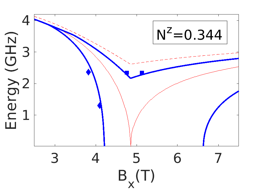
Figure 1: Low energy electronuclear modes of LiHoF₄, calculated at the experimentally relevant temperature of $T=50mK$, as a function of transverse field. The blue diamonds and squares indicate features in the inverse quality factors of experimentally measured magnon-polariton modes (see Fig. 2), which correspond to the modes shown above. The dashed red line shows the lowest single-ion excitation calculated using MF theory. Below this energy, the modes are collective excitations of the spins. In the RPA, considering a needle shaped sample, one finds that this mode softens to zero at the quantum critical point of the system (solid red line). In a sample with a non-zero demagnetization factor, a uniform longitudinal ac field gaps the soft mode leading to the upper-mode shown in dark blue. The soft mode is then a magnetostatic mode which nulls out shape effects. In addition there is a low energy Walker mode that softens to zero prior to the bulk phase transition. The modes shown in dark blue correspond to a sample with a demagnetization factor of $N^{z}=0.344$.

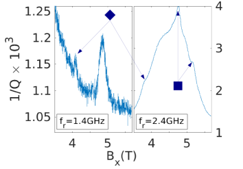
Figure 2: Inverse quality factor of the magnon-polariton mode of LiHoF₄ in a $f_{r}=1.4GHz$ and $f_{r}=2.4GHz$ resonator, plotted as a function of transverse field. The blue diamonds indicate features in $1/Q$ corresponding to an electronuclear mode having lower energy than the soft mode which governs quantum criticality in the bulk of the LiHoF₄ system. The blue squares indicate features in $1/Q$ which correspond to a uniform (Kittel) mode which is gapped by demagnetization field fluctuations. These data points are plotted along with the low energy electronuclear modes of LiHoF₄ in Fig. 1.

In Fig. 1, we plot low frequency modes of LiHoF₄ calculated at the experimentally relevant temperature of $T=50mK$. The MF/RPA theory overestimates the critical transverse field by $0.42$ Tesla. Interactions between fluctuations neglected in the RPA will lower the result for $B_{x}^{c}$. In the following, to compare the calculated data with experimental results, we simply downshift the transverse field, $B_{x}\rightarrow B_{x}-0.42T$. The dashed red line in the figure shows the lowest single-ion excitation calculated using MF theory. In the RPA, this mode softens to zero at the critical point of the system (the solid red line). In a needle shaped sample ($N^{z}=0$), the soft mode is a uniform (Kittel) mode, whereas if $N^{z}\neq 0$, the soft mode is an inhomogeneous (Walker) mode. With $N^{z}\neq 0$, the uniform mode is gapped by demagnetization field fluctuations, leading to the upper mode shown in blue. The lower mode shown in blue, which softens to zero prior to the critical point of the bulk of the material, is an inhomogeneous magnetostatic mode stemming from variations in the system’s magnetization.

The blue diamonds shown in Fig. 1 correspond to features seen in the inverse quality factor of a polariton mode present when LiHoF₄ is placed in a microwave resonator. The magnon-polariton propagator, $D_{mp}(\tau)=\langle T_{\tau}[a^{\dagger}(\tau)+a(\tau)](a^{\dagger}+a)\rangle$, determines propagation of photons through the resonator [41]. In Matsubara frequency space ($z=i\omega_{n}=i2\pi n/\beta$), one finds that

$$D_{mp}(z)=-\frac{2\omega_{r}}{\beta}\biggr{[}\frac{1}{z^{2}-\omega_{r}^{2}+g_{c}^{2}\chi(z)}\biggr{]}.$$ (125)

The (longitudinal) dynamic susceptibility of the spins is given by $\chi(z)=\chi_{\bm{k}=0}^{zz}(z)$, and the coupling, $g_{c}=\eta\omega_{r}\sqrt{4\pi\rho_{s}J_{D}}$, is proportional to the filling factor of the resonator $\eta$, and its frequency. The poles of this function determine the magnon-polariton modes which transmit light through a resonator.

For a resonator with frequency $\omega_{r}=2\pi f_{r}$, the measured magnon-polariton mode follows from $\omega_{mp}=\sqrt{\omega_{r}^{2}-g_{c}^{2}\chi^{\prime}(\omega_{mp})}$. The real component of the dynamic susceptibility reduces the resonant frequency of the resonator. Setting $z=i\omega_{n}\rightarrow\omega+i\Gamma_{r}/2$, where $\Gamma_{r}$ is the bare linewidth of the resonator mode, one finds the linewidth of the polariton mode to be $\Gamma_{mp}=\Gamma_{r}+g_{c}^{2}\chi^{\prime\prime}(\omega_{mp})/\omega_{mp}$. The absorptive component of the dynamic susceptibility increases the linewidth of the magnon-polariton mode, and hence, its inverse quality factor $1/Q=\Gamma_{mp}/\omega_{mp}$. The inverse quality factors for resonators with $f_{r}=1.4GHz$ and $f_{r}=2.4GHz$ are shown in Fig. 2.

In the $f_{r}=1.4GHz$ data set there is a clear resonance at the expected frequency of the lower Walker mode, viz., at the transverse field value where the lower Walker mode cuts through the magnon-polariton mode. The more prominent peak to its right corresponds to absorption by the soft mode and at the critical point of the system. In the $f_{r}=2.4GHz$ data set, at a particular transverse field value, there is overlapping absorption due to different modes, confounding the identification of the resonances. The rightmost shoulder in the $2.4GHz$ data set is in good agreement with the gapped uniform mode in the paramagnetic phase of the system, and the dominant peak agrees well with this mode in the ferromagnetic phase. The broad shoulder left of the dominant peak in the $2.4GHz$ data set corresponds to the soft mode, and the lower shoulder, indicated by a blue diamond, is in good agreement with the lower Walker mode calculated by the theory.

The experimental data sets shown were chosen because they provide the best evidence for the modes calculated in this paper. In other data sets, for resonators at other frequencies, the evidence for the modes shown in dark blue in Fig. 1 is less compelling. As previously noted, identification of the modes is difficult when there are multiple overlapping resonances in $1/Q$. The magnitude of the resonances will also depend on the spectral weights, and quantum coherence, of the modes, which we have not considered here. The experimental data for the magnetostatic modes calculated in this paper are not conclusive; however, the data are consistent with the theoretical analysis. We leave refinements of the theory, and a more detailed experimental analysis of the modes, as a subject for future work.

VI Discussion and Outlook

We have presented a theory of quantum criticality and magnetostatic modes in dipolar, uniaxial, magnetic materials, taking into consideration shape effects due to the long range magnetic interactions. In the presence of an applied ac field, demagnetization field fluctuations gap the uniform (Kittel) mode present in systems having a non-zero demagnetization factor; however, quantum criticality persists with the soft mode being an inhomogeneous magnetostatic (Walker) mode which nulls out surface effects. Furthermore, in an applied ac field, static fluctuations in a system’s magnetization lead to a magnetostatic mode having lower energy then the soft mode that governs criticality in the bulk of the system. This may give rise to effects similar to the Griffiths’ phase effects present in dilute magnetic materials [35]. The theory has been applied to experimental data on LiHoF₄ in a microwave resonator.

A magnetic material will divide itself into domains which null out surface effects, so that the system has a well defined thermodynamic limit, in accord with Griffiths’ theorem [16]. A primary result of this paper is that there is a magnetostatic soft mode in quantum Ising systems having a non-zero demagnetization factor. This is similar to Griffiths’ theorem; we have found that surface effects are nulled out by the magnetostatic mode so that quantum criticality persists in the bulk of the magnet.

Both Griffiths’ theorem, and this paper, indicate that shape effects may be neglected in efforts to understand quantum criticality. This justifies the use of a needle shaped sample, having zero demagnetization field, in calculations meant to capture bulk quantum critical behavior. However, in an experiment, shape effects must be treated with care. Note that shape effects, or rather, the absence of shape effects, analyzed in this paper, and by Griffiths, are due to the long range dipole-dipole interactions in the system. This is distinct from finite size effects which have been considered in renormalization group analyses of magnetic systems’ critical behavior. Domains, and inhomogeneous magnetostatic modes, null out shape effects; however, the quantum critical behavior of a system is still subject to finite-sized scaling, which gaps the soft mode and rounds off divergences in the susceptibility present when one considers the critical behavior of a finite-sized system [42].

In early papers on electronuclear modes [37, 19], researchers considered ellipsoids magnetized along an easy axis of magnetization by a static applied field, with an isotropic hyperfine interaction. The applied ac field was taken to be orthogonal to the magnetization direction. Here, we consider the TFIM, in which quantum effects become important and the direction of magnetization is not along the easy axis. The ac magnetic probe is assumed to lie along the easy axis of the material as is necessary to measure the soft mode near the quantum critical point [28].

The modes calculated in this paper depend on the (magnetometric) demagnetization factor of the sample through $\delta\overline{h}_{d}^{z}=N^{z}\delta\overline{m}^{z}$. At the level of the RPA, the demagnetization factor depends only on the lattice structure and the shape of the sample. In this paper, we neglect interactions between fluctuations which lead to the material specific, and temperature dependent, demagnetization factor $N^{z}(\chi)$ [see Eq. (9)]. In our analysis of LiHoF₄, we neglect off-diagonal-dipolar (ODD) interactions, which have been shown to lead to better quantitative agreement between experimental and theoretical determinations of the system’s phase diagram [43, 44]. We leave these fluctuation effects as a subject for future research.

Our analysis of electronuclear magnetostatic modes in terms of the average demagnetization field and magnetization fluctuations is appropriate for microwave resonator experiments, in which the wavelength of the input and output photons is much larger than the sample size. A more thorough analysis of the magnetostatic modes present in a material may be carried out by assuming a particular domain structure. Such an approach has been utilized by Sigal et al. to analyze magnetostatic modes, and Polder-Smit domain wall resonances, in systems with stripe and bubble domain structures [45, 34, 46].

Alternatively, one may analyze magnetostatic modes numerically from a microscopic perspective, as in the paper by Puszkarski et al. [47]. These researchers consider a cubic nanograin (a cubic lattice of $N\times N\times N$ dipoles with up to $N=101$), with an isotropic dipolar interaction. The system is assumed to be magnetized in the $z$ direction, and magnetic fluctuations in the $xy$ planes are assumed to be uniform, in which case the propagation is along the $z$ direction. They find a series of magnetostatic modes including high energy bulk extended modes, and lower energy surface and bulk localized modes.

The most promising avenue for future research is, perhaps, the magnetostatic mode which softens to zero prior to the quantum critical point. We expect this to lead to local regions of magnetic order near the sample surface prior to the phase transition in which the bulk of the material becomes magnetized. We expect this to be a ubiquitous feature of the critical behavior of magnetic materials, the effects of which have not been analyzed theoretically, or measured in an experiment. A thorough understanding of shape effects in quantum magnets is necessary in order to advance our understanding of quantum criticality, and in the development of quantum technologies.

VII Acknowledgements

The author would like to thank M Libersky, DM Silevitch, and TF Rosenbaum, for use of their experimental data. The author would also like to thank S Geim and the Rosenbaum group for feedback and helpful discussions. Experimental work at the California Institute of Technology was supported by U.S. Department of Energy Basic Energy Sciences Grant No. DESC0014866.

Appendix A Dynamic susceptibility of the quantum Ising model

Consider the internal (shape independent) RPA susceptibility of a quantum Ising material which follows from Eq. (40). Setting $x=-i\omega/(\gamma\mu_{0})$, the matrix on the left-hand side of Eq. (40) is given by

$$\widehat{A}=\left[\begin{array}[]{ccc}x&H_{\emptyset}^{z}&0\\ -H_{\emptyset}^{z}&x&H^{x}-\Phi_{\emptyset}M^{x}\\ 0&-H^{x}&x\\ \end{array}\right],$$ (129)

and the RPA modes of the material follow from setting $\text{det}[A]=0$, or

$$x[x^{2}+(H_{\emptyset}^{z})^{2}+H^{x}(H^{x}-\Phi_{\emptyset}M^{x})]=0.$$ (130)

One finds a “longitudinal” zero mode, $\omega_{\parallel}=0$, where by “longitudinal” we mean in the direction of the MF magnetization, and a pair of transverse modes

$$\omega_{\perp}=\pm(\gamma\mu_{0})\sqrt{(H_{\emptyset}^{z})^{2}+H^{x}(H^{x}-\Phi_{\emptyset}M^{x})}.$$ (131)

This collective mode softens to zero at the critical point of the TFIM.

Assuming $\omega\neq 0$, one may invert $A$ to obtain the internal susceptibility of the system

$$\widehat{\chi}_{in}(\omega\neq 0)=\widehat{A}^{-1}\left[\begin{array}[]{ccc}0&M^{z}&0\\ -M^{z}&0&M^{x}\\ 0&-M^{x}&0\\ \end{array}\right].$$ (135)

One finds

$$\widehat{\chi}_{in}(\omega\neq 0)=\left[\begin{array}[]{ccc}\chi^{xx}&-i\kappa^{xy}&\chi^{xz}\\ i\kappa^{xy}&\chi^{yy}&-i\kappa^{yz}\\ \chi^{xz}&i\kappa^{yz}&\chi^{zz}\\ \end{array}\right],$$ (139)

where we have suppressed the frequency dependence on the right-hand side for brevity. For the diagonal components of the susceptibility tensor we have

$$\chi^{xx}=\frac{(\gamma\mu_{0})^{2}M^{z}H_{\emptyset}^{z}}{\omega_{\perp}^{2}-\omega^{2}}\quad\text{and}\quad\chi^{zz}=\frac{(\gamma\mu_{0})^{2}M^{x}H^{x}}{\omega_{\perp}^{2}-\omega^{2}},$$ (140)

and

$$\chi^{yy}=\frac{M^{x}}{H^{x}}\frac{\omega_{\perp}^{2}}{\omega_{\perp}^{2}-\omega^{2}}=\frac{M^{z}}{H_{\emptyset}^{z}}\frac{\omega_{\perp}^{2}}{\omega_{\perp}^{2}-\omega^{2}}.$$ (141)

For the off-diagonal components of the susceptibility one finds

$$\chi^{xz}=\chi^{zx}=-\frac{(\gamma\mu_{0})^{2}H_{\emptyset}^{z}M^{x}}{\omega_{\perp}^{2}-\omega^{2}}.$$ (142)

The remaining off-diagonal components are $\chi^{xy}=-\chi^{yx}=-i\kappa^{xy}$ and $\chi^{yz}=-\chi^{zy}=-i\kappa^{yz}$, with

$$\kappa^{xy}=\frac{\omega\gamma\mu_{0}M^{z}}{\omega_{\perp}^{2}-\omega^{2}}\quad\text{and}\quad\kappa^{yz}=\frac{\omega\gamma\mu_{0}M^{x}}{\omega_{\perp}^{2}-\omega^{2}}.$$ (143)

As one approaches the critical point of the TFIM, $M^{z}\rightarrow 0$ and $\omega_{\perp}\rightarrow 0$, hence both $\chi^{xx}$ and $\chi^{yy}$ vanish. In a spectroscopy experiment, one must measure $\chi^{zz}$ to see resonant absorption by the soft mode [28, 5]. For the off-diagonal components of the susceptibility, one has $\chi^{xy}=-\chi^{yx}$ and $\chi^{yz}=-\chi^{zy}$. This anti-symmetry leads to a cancellation in the Walker mode equation given by Eq. (65). As $\chi^{xz}=\chi^{zx}$, the Walker mode equation for the TFIM contains a term not present in the usual Walker mode equation in which the applied ac field is orthogonal to the direction of magnetization [17, 48].

We have derived the internal RPA susceptibility of the TFIM. The MF result, which follows from Eq. (26) is similar; one must simply replace the transverse RPA mode with the MF result, $\omega_{\perp}\rightarrow\omega_{\perp}^{MF}=\gamma\mu_{0}\sqrt{(H^{x})^{2}+(H_{\emptyset}^{z})^{2}}$. In the absence of the transverse field, considering an ac field orthogonal to the direction of magnetization, one obtains the usual Polder susceptibility tensor ($\chi_{MF}=\chi_{MF}^{xx}=\chi_{MF}^{yy}$ and $\kappa_{MF}=\kappa_{MF}^{xy}$)

$$\widehat{\chi}_{MF}(\omega\neq 0)=\left[\begin{array}[]{cc}\chi_{MF}&-i\kappa_{MF}\\ i\kappa_{MF}&\chi_{MF}\\ \end{array}\right],$$ (146)

where

$$\chi_{MF}=\frac{\omega_{0}\omega_{M}}{\omega_{0}^{2}-\omega^{2}}\quad\text{and}\quad\kappa_{MF}=\frac{\omega\omega_{M}}{\omega_{0}^{2}-\omega^{2}},$$ (147)

with $\omega_{0}=\gamma\mu_{0}H_{\emptyset}^{z}$ and $\omega_{M}=\gamma\mu_{0}M^{z}$.

We have determined the dynamic susceptibility of the quantum Ising model making use of the EOM of the spin operators. Alternatively, one may consider the connected, imaginary time ordered, correlation function, $G_{ij}^{\mu\nu}(\tau)=-\langle T_{\tau}\delta J_{i}^{\mu}(\tau)\delta J_{j}^{\nu}(0)\rangle$. Transforming to momentum and Matsubara frequency space, this function is related to the dynamic spin susceptibility by $\chi_{\bm{k},J}^{\mu\nu}(\omega)=-\beta G_{\bm{k}}^{\mu\nu}(i\omega_{r}\rightarrow\omega+i0^{+})$. The dimensionless susceptibility of the material is then $\chi_{\bm{k}}^{\mu\nu}(\omega)=4\pi J_{D}\rho_{s}\chi_{\bm{k},J}^{\mu\nu}(\omega)$ In the RPA, at zero wavevector, one finds the longitudinal component of the susceptibility to be

$$\chi_{RPA}^{zz}(\omega\neq 0)=\frac{\chi_{\emptyset}^{zz}(\omega\neq 0)}{1-\Phi_{\emptyset}\chi_{\emptyset}^{zz}(\omega\neq 0)},$$ (148)

where $\chi_{\emptyset}^{zz}$ is the MF susceptibility of a needle, and $\Phi_{\emptyset}=V_{\emptyset}/(4\pi J_{D}\rho_{s})$. The poles of Eq. (104) determine the RPA modes of the material, and their residues determine spectral weights.

Indeed, in terms of MF eigenstates and matrix elements,

$$\mathcal{H}_{MF,i} =\sum_{n}E_{n}|X_{n,i}\rangle\langle X_{n,i}|\quad\text{and}\quad$$ (149)

$$c_{mn} =\langle X_{m,i}|J_{i}^{z}|X_{n,i}\rangle,$$

where the $\{X_{n,i}\}$ are single-ion Hubbard operators, one finds

$$\chi_{\emptyset}^{zz}(\omega\neq 0)=\sum_{n>m}|c_{mn}|^{2}p_{mn}\frac{4\pi J_{D}\rho_{s}2E_{nm}}{E_{nm}^{2}-(\omega+i0^{+})^{2}},$$ (150)

where the $p_{mn}=p_{m}-p_{n}$ are differences between population factors $p_{n}=e^{-\beta E_{n}}/Z_{MF}$. A straightforward calculation shows the result for the susceptibility and the RPA mode energy is equivalent to the results given in Eqs. (131) and (140). The Green function approach is advantageous when dealing with electronuclear systems as it avoids the RPA decoupling of the electronic and nuclear spins inherent in the EOM approach.

Appendix B Electronuclear Walker modes in LiHoF₄

The effective, low temperature, Hamiltonian of the LiHoF₄ system is $\mathcal{H}=\mathcal{H}_{e}+\mathcal{H}_{hyp}$, where the electronic component of the Hamiltonian is [31, 32, 28]

$$\mathcal{H}_{e}=-\frac{1}{2}\sum_{i\neq j}V_{ij}^{zz}\sigma_{i}^{z}\sigma_{j}^{z}-\frac{\Delta}{2}\sum_{i}\sigma_{i}^{x}.$$ (151)

The LiHoF₄ electronic-spin operators are related to the effective spin-half operators describing the low temperature physics by

$$\left[\begin{array}[]{c}J^{x}\\ J^{y}\\ J^{z}\\ \end{array}\right]=\left[\begin{array}[]{c}C^{x}\\ C^{y}\\ 0\\ \end{array}\right]+\left[\begin{array}[]{ccc}C_{xx}&C_{xy}&0\\ C_{yx}&C_{yy}&0\\ 0&0&C_{zz}\\ \end{array}\right]\left[\begin{array}[]{c}\sigma^{x}\\ \sigma^{y}\\ \sigma^{z}\\ \end{array}\right].$$ (164)

A discussion of the model parameters is provided in Sec. V. The truncated hyperfine interaction is given by

$$\mathcal{H}_{hyp}=A\sum_{i}\bm{J}_{i}\cdot\bm{I}_{i},$$ (165)

where the coupling between the truncated spin operator [Eq. (164)] and the $I=7/2$ nuclear spins is $A=39.8mK$ [39].

The EOM for the electronic spins follows from

$$\frac{d}{dt}\bm{\sigma}_{i} =i[\mathcal{H}_{e},\bm{\sigma}_{i}]+i[\mathcal{H}_{hyp},\bm{\sigma}_{i}]$$ (166)

$$=\widehat{M}_{\sigma}\ \bm{\sigma}_{i}+\widehat{M}_{hyp}\ \bm{\sigma}_{i},$$

where

$$\widehat{M}_{\sigma}=\left[\begin{array}[]{ccc}0&2\sum_{j}V_{ij}\sigma_{j}^{z}&0\\ -2\sum_{j}V_{ij}\sigma_{j}^{z}&0&\Delta\\ 0&-\Delta&0\\ \end{array}\right].$$ (170)

Defining the hyperfine field acting on the electronic spins to be

$$\left[\begin{array}[]{c}\widetilde{\Delta}_{i}^{x}\\ \widetilde{\Delta}_{i}^{y}\\ \widetilde{h}_{i}^{z}\\ \end{array}\right]=-2A\left[\begin{array}[]{ccc}C_{xx}&C_{yx}&0\\ C_{xy}&C_{yy}&0\\ 0&0&C_{zz}\\ \end{array}\right]\left[\begin{array}[]{c}I_{i}^{x}\\ I_{i}^{y}\\ I_{i}^{z}\\ \end{array}\right],$$ (180)

the hyperfine component of the EOM is

$$\widehat{M}_{hyp}=\left[\begin{array}[]{ccc}0&\widetilde{h}_{i}^{z}&-\widetilde{\Delta}_{i}^{y}\\ -\widetilde{h}_{i}^{z}&0&\widetilde{\Delta}_{i}^{x}\\ \widetilde{\Delta}_{i}^{y}&-\widetilde{\Delta}_{i}^{x}&0\\ \end{array}\right].$$ (184)

The nuclear time evolution is determined by

$$\frac{d}{dt}\bm{I}_{i}=i[\mathcal{H}_{hyp},\bm{I}_{i}]=\widehat{M}_{hyp}^{I}\ \bm{I}_{i}.$$ (185)

Each nuclear spin is subject to an electronic field defined by

$$\left[\begin{array}[]{c}\widetilde{\Delta}_{n,i}^{x}\\ \widetilde{\Delta}_{n,i}^{y}\\ \widetilde{h}_{n,i}^{z}\\ \end{array}\right]=\left[\begin{array}[]{c}-AC_{x}-AC_{xx}\sigma_{i}^{x}-AC_{xy}\sigma_{i}^{y}\\ -AC_{y}-AC_{yx}\sigma_{i}^{x}-AC_{yy}\sigma_{i}^{y}\\ -AC_{zz}\sigma_{i}^{z}\\ \end{array}\right],$$ (192)

and the matrix governing the nuclear dynamics is

$$\widehat{M}_{hyp}^{I}=\left[\begin{array}[]{ccc}0&\widetilde{h}_{n,i}^{z}&-\widetilde{\Delta}_{n,i}^{y}\\ -\widetilde{h}_{n,i}^{z}&0&\widetilde{\Delta}_{n,i}^{x}\\ \widetilde{\Delta}_{n,i}^{y}&-\widetilde{\Delta}_{n,i}^{x}&0\\ \end{array}\right].$$ (196)

To proceed, we decouple the electronic and nuclear spins in the RPA so that $\langle\sigma_{i}^{\mu}\sigma_{j}^{\nu}\rangle=\langle\sigma_{i}^{\mu}\rangle\langle\sigma_{j}^{\nu}\rangle$ and $\langle\sigma_{i}^{\mu}I_{i}^{\nu}\rangle=\langle\sigma_{i}^{\mu}\rangle\langle I_{i}^{\nu}\rangle$. Transforming to Fourier space, the linearized EOM for fluctuations of the operator $\bm{X}_{i}=\{\bm{\sigma}_{i},\bm{I}_{i}\}$ is given by

$$\frac{d}{dt}\delta\bm{X}_{q}=\widehat{M}_{RPA}\ \delta\bm{X}_{q}.$$ (197)

The matrix governing the time evolution may be divided into electronic and nuclear sectors, and the mixing between the two, as in Eq. (104).

In the electronic sector, there is a hyperfine correction to the fields acting on the electronic spins. Defining the shifted fields as

$$\widetilde{\Delta}_{x} =\Delta-2A(C_{xx}\langle I^{x}\rangle_{\emptyset}+C_{yx}\langle I^{y}\rangle_{\emptyset})$$ (198)

$$\widetilde{\Delta}_{y} =-2A(C_{xy}\langle I^{x}\rangle_{\emptyset}+C_{yy}\langle I^{y}\rangle_{\emptyset})$$

$$\widetilde{h}_{z} =-2AC_{zz}\langle I^{z}\rangle_{\emptyset},$$

where $\langle\cdots\rangle_{\emptyset}$ denotes an average taken with respect to the MF Hamiltonian of a needle shaped sample, one finds the matrix governing the RPA level electronic dynamics to be

$$\widehat{M}_{e} =$$ (199)

$$\left[\begin{array}[]{ccc}0&\widetilde{h}_{z}+2V_{\emptyset}\langle\sigma^{z}\rangle_{\emptyset}&-\widetilde{\Delta}_{y}\\ -\widetilde{h}_{z}-2V_{\emptyset}\langle\sigma^{z}\rangle_{\emptyset}&0&\widetilde{\Delta}_{x}-2V_{q}\langle\sigma^{x}\rangle_{\emptyset}\\ \widetilde{\Delta}_{y}&-\widetilde{\Delta}_{x}&0\\ \end{array}\right].$$ (203)

With $\widetilde{\Delta}_{y}=0$, this corresponds to the usual dynamics of the transverse field Ising model with the applied field shifted by the nuclear spins (see Eq. 108). The $\widetilde{\Delta}_{y}$ component of the field is small, and we will neglect it in what follows.

In the nuclear sector, the effective field acting on the nuclear spins is (setting $\langle\sigma^{y}\rangle_{\emptyset}=0$)

$$\left[\begin{array}[]{c}\widetilde{\Delta}_{n}^{x}\\ \widetilde{\Delta}_{n}^{y}\\ \widetilde{h}_{n}^{z}\\ \end{array}\right]=\left[\begin{array}[]{c}-AC_{x}-AC_{xx}\langle\sigma^{x}\rangle_{\emptyset}\\ -AC_{y}-AC_{yx}\langle\sigma^{x}\rangle_{\emptyset}\\ -AC_{zz}\langle\sigma^{z}\rangle_{\emptyset}\\ \end{array}\right].$$ (210)

The matrix governing the time evolution of the nuclear spins is

$$\widehat{M}_{n}=\left[\begin{array}[]{ccc}0&\widetilde{h}_{n}^{z}&-\widetilde{\Delta}_{n}^{y}\\ -\widetilde{h}_{n}^{z}&0&\widetilde{\Delta}_{n}^{x}\\ \widetilde{\Delta}_{n}^{y}&-\widetilde{\Delta}_{n}^{x}&0\\ \end{array}\right].$$ (214)

The matrices $\widehat{M}_{e}$ and $\widehat{M}_{n}$ determine MF/RPA precession of the electronic and nuclear spins about their MFs. The resulting modes are mixed by

$$\widehat{M}_{en}=$$ (215)

$$\left[\begin{array}[]{ccc}2AC_{xy}\langle\sigma^{z}\rangle_{\emptyset}&2AC_{yy}\langle\sigma^{z}\rangle_{\emptyset}&0\\ -2AC_{xx}\langle\sigma^{z}\rangle_{\emptyset}&-2AC_{yx}\langle\sigma^{z}\rangle_{\emptyset}&2AC_{zz}\langle\sigma^{x}\rangle_{\emptyset}\\ -2AC_{xy}\langle\sigma^{x}\rangle_{\emptyset}&-2AC_{yy}\langle\sigma^{x}\rangle_{\emptyset}&0\\ \end{array}\right],$$ (219)

and

$$\widehat{M}_{ne}=\left[\begin{array}[]{ccc}AC_{yx}\langle I^{z}\rangle_{\emptyset}&AC_{yy}\langle I^{z}\rangle_{\emptyset}&-AC_{zz}\langle I^{y}\rangle_{\emptyset}\\ -AC_{xx}\langle I^{z}\rangle_{\emptyset}&-AC_{xy}\langle I^{z}\rangle_{\emptyset}&AC_{zz}\langle I^{x}\rangle_{\emptyset}\\ -AC_{yx}\langle I^{x}\rangle_{\emptyset}+AC_{xx}\langle I^{y}\rangle_{\emptyset}&-AC_{yy}\langle I^{x}\rangle_{0}+AC_{xy}\langle I^{y}\rangle_{\emptyset}&0\\ \end{array}\right].$$ (223)

These coupled equations determine the RPA modes of a needle-shaped sample of LiHoF₄.

In order calculate Walker modes in an arbitrarily shaped sample, we add an internal drive field to Eq. (151),

$$\mathcal{H}_{e}(t) =\mathcal{H}_{e}$$ (224)

$$-\sum_{i}\delta\bm{h}_{in,i}^{e}(t)\cdot\bm{\sigma}_{i}-\sum_{i}\delta\bm{h}_{in,i}^{n}(t)\cdot\bm{I}_{i},$$

where $\delta\bm{h}_{in,i}^{e,n}(t)=\delta\bm{h}_{a}^{z}(t)+\delta\bm{h}_{d,i}^{e,n}(t)$ includes an ac drive field and time dependent demagnetization field fluctuations. Considering a single Fourier component of the drive field and the resulting magnetization fluctuations, the RPA EOM is

$$i\omega\delta\bm{X}_{q}=\widehat{M}_{RPA}\ \delta\bm{X}_{q}+\widehat{M}_{\delta}\ \delta\bm{h}_{q},$$ (225)

where $\delta\bm{h}_{q}=(\delta\bm{h}_{in,q}^{e},\delta\bm{h}_{in,q}^{n})$, and

$$\widehat{M}_{\delta}=$$ (226)

$$\left[\begin{array}[]{cccccc}0&-2\langle\sigma^{z}\rangle_{\emptyset}&0&0&0&0\\ 2\langle\sigma^{z}\rangle_{\emptyset}&0&-2\langle\sigma^{x}\rangle_{\emptyset}&0&0&0\\ 0&2\langle\sigma^{x}\rangle_{\emptyset}&0&0&0&0\\ 0&0&0&0&-\langle I^{z}\rangle_{\emptyset}&\langle I^{y}\rangle_{\emptyset}\\ 0&0&0&\langle I^{z}\rangle_{\emptyset}&0&-\langle I^{x}\rangle_{\emptyset}\\ 0&0&0&-\langle I^{y}\rangle_{\emptyset}&\langle I^{x}\rangle_{\emptyset}&0\\ \end{array}\right].$$ (233)

This is an electronuclear generalization of Eq. (40) applied to LiHoF₄.

The field and magnetization fluctuations are related to the parameters in the microscopic model by

$$\delta\bm{M}_{e}=2\rho_{s}\gamma_{e}C_{zz}\ \langle\delta\bm{\sigma}\rangle \delta\bm{M}_{n}=\rho_{s}\gamma_{n}\ \langle\delta\bm{I}\rangle$$ (234)

$$\delta h_{e}^{z}=\frac{C_{zz}\gamma_{e}\mu_{0}}{2}\ \delta H_{e}^{z} \delta\bm{h}_{n}=\frac{\gamma_{n}\mu_{0}}{2}\ \delta\bm{H}_{n}.$$

For a uniform magnetic fluctuation ($q=0$) across a sample with demagnetization factor $N^{z}$, the average, longitudinal, electronic and nuclear demagnetization field fluctuations are $(\delta\overline{H}_{d}^{e,n})^{z}=-N^{z}\delta\overline{M}_{e,n}^{z}$. This leads to

$$\delta\overline{h}_{d,e}^{z} =-\gamma_{e}^{2}\rho_{s}\mu_{0}C_{zz}^{2}N^{z}\langle\delta\sigma^{z}\rangle_{\emptyset}\quad\text{and}\quad$$ (235)

$$\delta\overline{h}_{d,n}^{z} =-\frac{\gamma_{n}^{2}\rho_{s}\mu_{0}}{2}N^{z}\langle\delta I^{z}\rangle_{\emptyset}.$$

In LiHoF₄, $\gamma_{e}^{2}\rho_{s}\mu_{0}=4\pi J_{D}\rho_{s}=0.1699K$ and $\gamma_{n}^{2}\rho_{s}\mu_{0}=4.5782\times 10^{-8}K$. As $\delta\overline{h}_{d,n}^{z}\ll\delta\overline{h}_{e,n}^{z}$, we will drop the nuclear demagnetization field fluctuations from subsequent analysis. The electronic demagnetization field fluctuations may be written

$$\delta\overline{h}_{d,e}^{z}=-f_{d}\langle\delta\sigma^{z}\rangle_{\emptyset}\quad\text{with}\quad f_{d}=4\pi\rho_{s}J_{D}C_{zz}^{2}N^{z}.$$ (236)

The ac demagnetization field fluctuations are proportional to the ac fluctuations in the system’s magnetization.

To proceed, we rewrite Eq. (225) as ($q=0$)

$$\widehat{M}_{W}\ \delta\bm{X}=\widehat{M}_{\delta}\ \delta\bm{h}_{a}.$$ (237)

This is an electronuclear generalization of Eq. (56). The modes of the system follow from

$$\text{det}\{\widehat{M}_{W}\}=\text{det}\Biggr{\{}\left[\begin{array}[]{cc}\widehat{M}_{W}^{e}&\widehat{M}_{en}\\ \widehat{M}_{ne}&\widehat{M}_{W}^{n}\\ \end{array}\right]\Biggr{\}}=0.$$ (240)

The off-diagonal components are the same as in $\widehat{M}_{RPA}$, and the nuclear demagnetization field fluctuations are negligibly small so that $\widehat{M}_{W}^{n}\approx\widehat{M}_{n}$. The electronic demagnetization field fluctuations lead to

$$\widehat{M}_{W}^{e}=\left[\begin{array}[]{ccc}-i\omega&\widetilde{h}_{z}+2V_{\emptyset}\langle\sigma^{z}\rangle_{\emptyset}&-\widetilde{\Delta}_{y}\\ -\widetilde{h}_{z}-2V_{\emptyset}\langle\sigma^{z}\rangle_{\emptyset}&-i\omega&\widetilde{\Delta}_{x}-2(V_{\emptyset}-f_{d})\langle\sigma^{x}\rangle_{\emptyset}\\ \widetilde{\Delta}_{y}&-\widetilde{\Delta}_{x}&-i\omega\\ \end{array}\right].$$ (244)

The primary difference between the shape-independent RPA modes and the Walker modes is in $\widehat{M}_{W}^{e}$.

One finds that the average demagnetization field fluctuation resulting from the applied ac field shifts the interaction strength

$$V_{\emptyset} \rightarrow V_{0}=V_{\emptyset}-f_{d}$$ (245)

$$=C_{zz}^{2}\rho_{s}J_{D}\biggr{[}\frac{4\pi}{3}+\lambda_{dip}-4\pi\lambda_{ex}-4\pi N^{z}\biggr{]}$$

in the right-most component of $\widehat{M}_{W}^{e}$. This gaps the uniform (Kittel) mode present in the material. As discussed in Sec. III, a magnetostatic mode mirroring the electronic demagnetization field fluctuation will soften to zero, governing the bulk critical behavior of the system. In addition, as discussed in Section III.1, a magnetostatic mode due to static variations in the system’s magnetization will soften to zero prior to the bulk phase transition. As discussed in Appendix A, one may make use of the RPA susceptibility tensor to determine the electronuclear magnetostatic modes of the material. This approach avoids the RPA decoupling of the electronic and nuclear spins inherent in the EOM approach.

Appendix C Electronuclear dynamics and frequency pulling

Early work on electronuclear dynamics was carried out be de Gennes et al [37]. They found that interactions between nuclear moments mediated by the electronic spins (the Suhl-Nakamura interaction [49, 50]) lead to a reduction in the energy of the nuclear mode, known as frequency pulling. Their results were used by Blocker to analyze Walker modes in electronuclear systems [19]. These authors consider a ferromagnet magnetized in the $z$ direction by an applied field, with an isotropic hyperfine interaction, subject to an ac field orthogonal to the direction of magnetization. For reference, we review the frequency pulling result making use of the notation in the current paper.

Consider the dipolar Ising model in a longitudinal field with an isotropic hyperfine interaction

$$\mathcal{H}=-\frac{1}{2} \sum_{i\neq j}V_{ij}^{zz}J_{i}^{z}J_{j}^{z}$$ (246)

$$+h\sum_{i}(J_{i}^{z}-\gamma I_{i}^{z})+A\sum_{i}\bm{J}_{i}\cdot\bm{I}_{i},$$

where $\gamma=|\gamma_{n}/\gamma_{e}|$ is the ratio of nuclear and electronic gyromagnetic rations, and the interaction between spins is dipolar, $V_{ij}^{zz}=J_{D}D_{ij}^{zz}$. The total moment at each site is given by $\bm{\mu}=\gamma_{e}\bm{J}+\gamma_{n}\bm{I}$ ($\hbar=1$), and the local magnetization is $\bm{M}=\rho_{s}\bm{\mu}=\bm{M}_{e}+\bm{M}_{n}$. Assuming a uniformly magnetized ellipsoid and treating the interaction in MF theory, the single-ion Hamiltonian may be written

$$\mathcal{H}_{MF}=-\frac{\mu_{0}}{\rho_{s}}[H_{loc}^{z}M_{e}^{z}+H_{n}^{z}M_{n}^{z}+\alpha\bm{M}_{e}\cdot\bm{M}_{n}].$$ (247)

The local field experienced by the electronic moments is

$$H_{loc}^{z}=-\frac{h}{\mu_{0}\gamma_{e}}+\Phi_{0}M_{e}^{z},$$ (248)

where $\Phi_{0}=D_{0}^{zz}/4\pi\rho_{s}$ (see Eq. 4). The longitudinal nuclear field and hyperfine coupling are

$$H_{n}^{z}=-\frac{h}{\gamma_{e}\mu_{0}}\quad\text{and}\quad\alpha=-\frac{A}{\mu_{0}\rho_{s}\gamma_{e}\gamma_{n}}.$$ (249)

Note that $\gamma_{e}=-g\mu_{B}<0$, so that $\alpha$ and the fields are greater than zero. We proceed by analyzing the EOM for the coupled electronic and nuclear magnetizations.

The coupled equations for the electronic and nuclear magnetizations are

$$\frac{d}{dt}\bm{M}_{e}(t) =\mu_{0}\gamma_{e}\bm{M}_{e}(t)\times[H_{loc}^{z}+\alpha\bm{M}_{n}(t)]\quad\text{and}$$ (250)

$$\frac{d}{dt}\bm{M}_{n}(t) =\mu_{0}\gamma_{n}\bm{M}_{n}(t)\times[H_{n}^{z}+\alpha\bm{M}_{e}(t)].$$

In a transverse ac field, we assume small transverse motions of the electronic spins so that $\bm{M}_{e}(t)=\bm{M}_{e}+\delta\bm{m}_{e}(t)=(\delta m_{e}^{x}(t),\delta m_{e}^{y}(t),M_{e}^{z})$. At the MF level of approximation, we neglect fluctuations in the local field $H_{loc}^{z}$ (see Eq. 26). Writing the nuclear spin magnetization as $\bm{M}_{n}(t)=\bm{M}_{n}+\delta\bm{m}_{n}(t)$, the linearized EOM for the electronic magnetization is

$$\bm{M}_{e}\times(H_{loc}^{z}+\alpha\bm{M}_{n})=0\quad\text{and}$$ (251)

$$\frac{d}{dt}\delta\bm{m}_{e}=\mu_{0}\gamma_{e}[\delta\bm{m}_{e}\times(H_{loc}^{z}+\alpha\bm{M}_{n})+\alpha\bm{M}_{e}\times\delta\bm{m}_{n}],$$

where in the the final line we have suppressed the time dependence of the electronic and nuclear magnetization fluctuations, $\delta\bm{m}_{e,n}(t)$.

As $\bm{M}_{e}=(0,0,M_{e}^{z})$, the first expression in Eq. (251) tells us that $\bm{M}_{n}=(0,0,M_{n}^{z})$. In a transverse ac field, we consider transverse fluctuations about the average magnetization, $\bm{M}_{n}(t)=(\delta m_{n}^{x}(t),\delta m_{n}^{y}(t),M_{n}^{z})$. It is assumed by de Gennes et al. that the electrons follow the field $H_{loc}^{z}+\alpha\bm{M}_{n}(t)$ adiabatically so that $\bm{M}_{e}(t)\parallel[H_{loc}^{z}+\alpha\bm{M}_{n}(t)]$ [37]. The equation for the electronic fluctuations is then

$$\delta\bm{m}_{e}\times(H_{loc}^{z}+\alpha\bm{M}_{n})+\alpha\bm{M}_{e}\times\delta\bm{m}_{n}=0.$$ (252)

In terms of the circularly polarized wave $\delta m_{e}^{+}=\delta m_{x}+i\delta m^{y}$, one finds

$$\delta m_{e}^{+}=\frac{\alpha M_{e}^{z}}{H_{loc}^{z}+\alpha M_{n}^{z}}\delta m_{n}^{+}.$$ (253)

This is equivalent to Eq. 2.2 of de Gennes et al. with two caveats: 1) The local field considered by de Gennes et al. includes an applied field and an anisotropy field. Here, we consider an Ising system, and the local field includes an applied field as well as the dipolar MF. 2) The hyperfine correction to the local field in the denominator of Eq. (253) is not included in the work of de Gennes et al.. If the hyperfine interaction is weak, this term will be negligibly small and the two equations are equivalent; however, in materials with strong hyperfine couplings, such as LiHoF₄, this term should not be neglected. Making use of Eq. (253), we proceed by analyzing the EOM for the nuclear magnetization.

The linearized EOM for fluctuations in the nuclear magnetization is

$$\frac{d}{dt}\delta\bm{m}_{n}=\mu_{0}\gamma_{n}[\delta\bm{m}_{n}\times(H_{n}^{z}+\alpha\bm{M}_{e})+\alpha\bm{M}_{n}\times\delta\bm{m}_{e}]$$ (254)

For a circularly polarized nuclear magnetic fluctuation, $\delta m_{n}^{+}=\delta m_{n}^{x}+i\delta m_{n}^{y}$, one finds

$$\frac{d}{dt}\delta m_{n}^{+}=i\mu_{0}\gamma_{n}[\delta m_{e}^{+}\alpha M_{n}^{z}-\delta m_{n}^{+}(H_{n}^{z}+\alpha M_{e}^{z})].$$ (255)

Considering a single Fourier component of the nuclear magnetization fluctuation, $\delta m_{n}^{+}(t)=\delta m_{n}^{+}e^{i\omega t}$, and making use of equation (253), we find the nuclear resonance frequency to be

$$\omega_{n} =-\mu_{0}\gamma_{n}\biggr{[}H_{n}^{z}+\alpha M_{e}^{z}\biggr{(}1-\eta\frac{M_{n}^{z}}{M_{e}^{z}}\biggr{)}\biggr{]}$$ (256)

$$\quad\text{with}\quad\eta=\frac{\alpha M_{e}^{z}}{H_{loc}^{z}+\alpha M_{n}^{z}}.$$

This is in agreement with Eq. 2.4 of de Gennes et al. apart from the additional hyperfine contribution in the denominator of $\eta$. As previously noted, if the hyperfine coupling is small $\alpha M_{n}^{z}$ may be neglected. In the absence of the interactions between the nuclear spins mediated by the electronic spins (the Suhl-Nakamura interaction), the nuclear spins would precess about the applied field and electronic MF with frequency $\omega_{n}=-\mu_{0}\gamma_{n}(H_{n}^{z}+\alpha M_{e}^{z})$. The Suhl-Nakamura interaction leads to a reduction in the frequency of the nuclear mode known as frequency pulling.

In terms of the parameters of the original spin Hamiltonian, the nuclear resonance frequency is (note $\langle J^{z}\rangle_{MF}\leq 0$ and $\langle I^{z}\rangle_{MF}\geq 0$)

$$\omega_{n}=-\gamma h+A\langle J^{z}\rangle_{MF}\biggr{[}\frac{h_{MF}}{h_{MF}+A\langle I^{z}\rangle_{MF}}\biggr{]},$$ (257)

where $h_{MF}=h-V_{0}^{zz}\langle J^{z}\rangle_{MF}$. One may make use of the adiabatic approximation to analyze electronuclear modes in the TFIM with an anisotropic hyperfine interaction; however, the resulting equations become rather complicated. In this paper, we have considered the $6\times 6$ EOM for the coupled electronic and nuclear spins, subject to a longitudinal ac field, and solved for the electronuclear modes numerically.

References

- Dutta et al. [2015] A. Dutta, G. Aeppli, B. K. Chakrabarti, U. Divakaran, T. F. Rosenbaum, and D. Sen, Quantum Phase Transitions in Transverse Field Spin Models, 1st ed. (Cambridge University Press, 2015).
- Suzuki et al. [2013] S. Suzuki, J. Inoue, and B. Chakrabarti, Quantum Ising Phases and Transitions in Transverse Ising Models, 2nd ed. (Springer Heidelberg New York Dordrecht London, 2013).
- Sachdev [1999] S. Sachdev, Quantum Phase Transitions, 1st ed. (Cambridge University Press, 1999).
- Bitko et al. [1996] D. Bitko, T. F. Rosenbaum, and G. Aeppli, Quantum Critical Behaviour for a Model Magnet, Phys. Rev. Lett. 77, 940 (1996).
- Libersky et al. [2021] M. Libersky, R. D. McKenzie, D. M. Silevitch, P. C. E. Stamp, and T. F. Rosenbaum, Direct Observation of Collective Electronuclear Modes about a Quantum Critical Point, Phys. Rev. Lett. 127, 207202 (2021).
- Wendl et al. [2022] A. Wendl, H. Eisenlohr, F. Rucker, C. Duvinage, M. Kleinhans, M. Vojta, and C. Pfleiderer, Emergence of mesoscale quantum phase transitions in a ferromagnet, Nature 609, 65 (2022).
- Tabuchi et al. [2016] Y. Tabuchi, S. Ishino, A. Noguchi, T. Ishikawa, R. Yamazaki, K. Usami, and Y. Nakamura, Quantum magnonics: The magnon meets the superconducting qubit, C. R. Physique 17, 729 (2016).
- Lachance-Quirion et al. [2019] D. Lachance-Quirion, Y. Tabuchi, A. Gloppe, K. Usami, and Y. Nakamura, Hybrid quantum systems based on magnonics, Applied Physics Express 12, 070101 (2019).
- Harder and Hu [2018] M. Harder and C. M. Hu, Cavity Spintronics: An Early Review of Recent Progress in the Study of Magnon-Photon Level Repulsion, Solid State Physics 69, 47 (2018).
- Rameshti et al. [2022] B. Z. Rameshti, S. V. Kusminskiy, J. A. Haigh, K. Usami, D. Lachance-Quirion, Y. Nakamura, C.-M. Hu, H. X. Tang, G. E. W. Bauer, and Y. M. Blanter, Cavity magnonics, Physics Reports 979, 1 (2022).
- Yuan et al. [2022] H. Y. Yuan, Y. Cao, A. Kamra, R. A. Duine, and P. Yan, Quantum magnonics: When magnon spintronics meets quantum information science, Physics Reports 965, 1 (2022).
- Lachance-Quirion et al. [2020] D. Lachance-Quirion, S. P. Wolski, Y. Tabuchi, S. Kono, K. Usami, and Y. Nakamura, Entanglement-based single-shot detection of a single magnon with a superconducting qubit, Science 367, 425 (2020).
- Hisatomi et al. [2016] R. Hisatomi, A. Osada, Y. Tabuchi, T. Ishikawa, A. Noguchi, R. Yamazaki, K. Usami, and Y. Nakamura, Bidirectional conversion between microwave and light via ferromagnetic magnons, Phys. Rev. B 93, 174427 (2016).
- Cherepanov et al. [1993] V. Cherepanov, I. Kolokolov, and V. L’Vov, The Saga of YIG: Spectra, thermodynamics, Interaction and Relaxation of Magnons in a Complex Magnet, Phyics Reports 229, 81 (1993).
- Serga et al. [2010] A. A. Serga, A. V. Chumak, and B. Hillebrands, YIG magnonics, J. Phys. D: Appl. Phys. 43, 1 (2010).
- Griffiths [1968] R. B. Griffiths, Free Energy of Interacting Magnetic Dipoles, Physical Review 176, 655 (1968).
- Walker [1957] L. R. Walker, Magnetostatic Modes in Ferromagnetic Resonance, Phys. Rev. 105, 390 (1957).
- Walker [1958] L. R. Walker, Resonant Modes of Ferromagnetic Spheroids, Journal of Applied Physics 29, 318 (1958).
- Blocker [1967] T. G. Blocker, Coupled Electron-Nuclear Magnetostatic Modes in Magnetic Materials, Physical Review 154, 446 (1967).
- Levy [1968] P. M. Levy, Shape Dependence of the Thermodynamic Properties of Magnetic Systems, Phys. Rev. 170, 595 (1968).
- Aharoni [1996] A. Aharoni, Introduction to the Theory of Ferromagnetism, 2nd ed. (Oxford University Press, 1996).
- Twengström et al. [2020] M. Twengström, L. Bovo, O. A. Petrenko, S. T. Bramwell, and P. Henelius, LiHoF4: Cuboidal Demagnetizing Factor in an Ising Ferromagnet, Phys. Rev. B 102, 144426 (2020).
- Kittel [1946] C. Kittel, Theory of the Structure of Ferromagnetic Domains in Films and Small Particles, Phys. Rev. 70, 965 (1946).
- Kooy and Enz [1960] C. Kooy and U. Enz, Experimental and Theoretical Study of the Domain Configuration in Thin Layers of BaFe12O19, Philips Res. Repts. 15, 7 (1960).
- Cooke et al. [1975] A. H. Cooke, D. A. Jones, J. F. A. Silva, and M. R. Wells, Ferromagnetism in LiHoF4 1: Magnetic Measurements, J. Phys. C 8, 4083 (1975).
- Mennenga et al. [1984] G. Mennenga, L. J. de Jongh, and W. J. Huiskamp, Field Dependent Specific Heat Study of the Dipolar Ising Ferromagnet LiHoF4, J. Magn. Magn. Mat. 44, 59 (1984).
- Jensen and Mackintosh [1991] J. Jensen and A. R. Mackintosh, Rare Earth Magnetism Structures and Excitations, 1st ed. (Clarendon Press - Oxford, 1991).
- McKenzie and Stamp [2018] R. D. McKenzie and P. C. E. Stamp, Thermodynamics of a quantum Ising system coupled to a spin bath, Phys. Rev. B 97, 214430 (2018).
- de Gennes [1963] P. G. de Gennes, Collective Motions of Hydrogen Bonds, Solid State Communications 1, 132 (1963).
- Brout et al. [1966] R. Brout, K. A. Müller, and H. Thomas, Tunnelling and Collective Excitations in a Microscopic Model of Ferroelectricity, Solid State Communications 4, 507 (1966).
- Chakraborty et al. [2004] P. B. Chakraborty, P. Henelius, H. Kjønsberg, A. W. Sandvik, and S. M. Girvin, Theory of the magnetic phase diagram of LiHoF4, Phys. Rev. B 70, 144411 (2004).
- Tabei et al. [2008] S. M. A. Tabei, M. J. P. Gingras, Y. J. Kao, and T. Yavors’kii, Perturbative Quantum Monte Carlo Study of LiHoF4 in a Transverse Magnetic Field, Phys. Rev. B 78, 184408 (2008).
- Twengström et al. [2017] M. Twengström, L. Bovo, M. J. P. Gingras, S. T. Bramwell, and P. Henelius, Microscopic aspects of magnetic lattice demagnetizing factors, Phys. Rev. Mat. 1, 044406 (2017).
- Sigal [1979] M. A. Sigal, Ferromagnetic Resonance Absorption in a Thin Uniaxial Platelet with Stripe Domain Structure Magnetized along the Easy Axis, phys. stat. sol. (a) 51, 151 (1979).
- Griffiths [1969] R. B. Griffiths, Nonanalytic behaviour above the critical point in a random Ising ferromagnet, Physical Review 23, 17 (1969).
- Meyer et al. [1989] P. Meyer, J. Pommier, and J. Ferré, Magnetic obvservation of domains at low temperature in the transparent ferromagnet LiHoF4, SPIE Electro-Optic and Magneto-Optic Materials and Applications 1126, 93 (1989).
- de Gennes et al. [1963] P. G. de Gennes, P. A. Pincus, F. Hartmann-Boutron, and J. M. Winter, Nuclear Magnetic Resonance Modes in Magnetic Material. 1. Theory, Phys. Rev. 129, 1105 (1963).
- Rønnow et al. [2007] H. M. Rønnow, J. Jensen, R. Parthasarathy, G. Aeppli, T. F. Rosenbaum, D. F. McMorrow, and C. Kraemer, Magnetic Excitations Near the Quantum Phase Transition in the Ising Ferromagnet LiHoF4, Phys. Rev. B 75, 055426 (2007).
- Magario et al. [1980] J. Magario, J. Tuchendler, P. Beauvillain, and I. Laursen, EPR Experiments in LiTbF4, LiHoF4, and LiErF4 at Submillimeter Frequencies, Phys. Rev. B 21, 18 (1980).
- Aharoni [1998] A. Aharoni, Demagnetization factors for rectangular ferromagnetic prisms, Journal of Applied Physics 83, 3432 (1998).
- McKenzie et al. [2022] R. D. McKenzie, M. Libersky, D. M. Silevitch, and T. F. Rosenbaum, Theory of magnon polaritons in quantum Ising materials, Phys. Rev. A 106, 043716 (2022).
- Goldenfeld [1992] N. Goldenfeld, Lectures on Phase Transitions and the Renormalization Group, 1st ed. (Westview Press, 1992).
- Dollberg et al. [2022] T. Dollberg, J. C. Andresen, and M. Schechter, The effect of intrinsic quantum fluctuations on the phase diagram of anisotropic dipolar magnets, Phys. Rev. B 105, 1 (2022).
- Dollberg and Schechter [2023] T. Dollberg and M. Schechter, LiHoF4 as a spin-half non-standard quantum Ising system, arXiv:2308.10095 , 1 (2023).
- Polder and Smit [1953] D. Polder and J. Smit, Resonance Phenomena in Ferrites, Rev. Mod. Phys. 25, 89 (1953).
- Sigal and Kostenko [1991] M. A. Sigal and V. I. Kostenko, Magnetostatic Modes in a Thin Uniaxial Platelet with Bubble Lattice at Normal Magnetization, phys. stat. sol. (a) 128, 219 (1991).
- Puszkarski et al. [2005] H. Puszkarski, M. Krawczyk, and J. C. S. L’evy, Localization properties of pure magnetostatic modes in a cubic nanograin, Phys. Rev. B 71, 014421 (2005).
- Stancil and Prabhakar [2009] D. D. Stancil and A. Prabhakar, Spin Waves Theory and Applications, 1st ed. (Springer, 2009).
- Suhl [1958] H. Suhl, Effective Nuclear Spin Interactions in Ferromagnets, Phys. Rev. 109, 606 (1958).
- Nakamura [1958] T. Nakamura, Indirect Coupling of Nuclear Spins in Antiferromagnet with Particular Reference to MnF2 at Very Low Temperatures, Progress of Theoretical Physics 20, 542 (1958).