Continuation of fixed points and bifurcations
from ODE to flow-kick disturbance models

Abstract

Some ODE models treat ecological disturbance as a continuous process, even disturbances such as fire that occur almost instantaneously on the timescale of system recovery. Alternatively, flow-kick models resolve disturbances as discrete impulses that change an ODE system’s state periodically in time. Here we compare the dynamics of continuously disturbed ODE models to those of flow-kick models with the same average disturbance rate. In the case that kicks are small and high-frequency, we find multiple similarities between continuous and analogous discrete disturbance models. First, we prove that flow-kick maps generate an analogous vector field in the limit as the period between kicks approaches zero. Second, we present conditions under which equilibria, saddle-node bifurcations, and transcritical bifurcations continue from ODE to flow-kick systems. On the other hand, we also provide numerical evidence that similarities between continuous and discrete disturbance models can break down as the period between kicks grows. We illustrate implications of these differences for climate change in a nonspatial Klausmeier model of vegetation and precipitation dynamics. We conclude that although ODEs may suffice to model high-frequency disturbances, resolving lower-frequency disturbances in time may be essential to effectively predicting their effects.

¹Carleton College, Northfield, MN, USA
²Mount Holyoke College, South Hadley, MA, USA
^∗corresponding author: kjmeyer@carleton.edu

Keywords: flow-kick systems, impulsive differential equations, ordinary differential equations

Introduction

Modeling disturbances in an ecosystem—or any system—requires choices along a number of axes. Disturbances can be treated as deterministic or stochastic; spatially homogeneous or heterogeneous; temporally continuous or discrete. While a model of wildfires on the scale of 1,000 km might include stochastic components and spatial heterogeneity, controlled burns on the scale of 100 meters might be reasonably modeled as deterministic and spatially uniform. We focus on the case of deterministic, nonspatial models and probe the third axis: whether disturbances occur continuously in time or at discrete time points. In particular, we ask how this choice impacts model predictions. Given that simple differential equations are used to model real-world disturbances that are markedly discrete in flavor, such as fire [1] and rainfall [2] events, is a discrete disturbance model worth the complexity cost?

To explore this question, we model disturbances continuously with ordinary differential equations (ODEs) and discretely with impulsive differential equations [3]. We focus on a subset of impulsive differential equations called flow-kick systems, which have emerged as a tool to study the interplay between discrete disturbance and continuous recovery when disturbances occur periodically in time [4, 5, 6]. A flow-kick map is built from two processes: a flow phase governed by an ODE and a discrete kick that delivers disturbance. This modeling structure appears under a variety of names in applications, including hurricane impacts on coral reefs [7], neurobiology of drug addiction [8], fires [9, 10, 6], seasonal grazing [11], biocontrol [12], and viral exposure [13]. Theoretical studies have also uncovered rich dynamic structures such as horseshoes and strange attractors that emerge from periodically kicking simple flows [14, 15, 16]. Packaging one cycle of flow-kick into a map on state space opens up study of disturbance dynamics to the theory of iterated maps, including fixed points (where disturbance and recovery balance) and bifurcations (potential tipping points). However, one typically lacks a closed form for the flow-kick map.

This added complexity of the discrete approach both motivates our comparison to continuous systems and poses a challenge for analyzing flow-kick maps—a challenge which we address analytically using Taylor expansions of the flow and numerically using the MatcontM continuation package. Using these tools, we present evidence that predictions are similar between continuous and discrete, high-frequency disturbance models, but that this similarity breaks down for lower frequencies. Thus using a discrete disturbance model may yield novel insights.

We outline our five main analytic results (boldfaced below) in the simple context of the logistic model of population growth

$$x^{\prime}=x(1-x)$$ (1)

disturbed by harvesting.

Figure 1 illustrates three disturbed logistic systems that feature the same average disturbance rate over time.

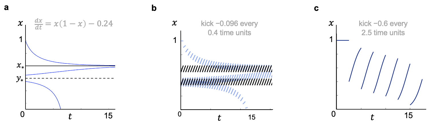
Figure 1: (a) Logistic minus continuous harvesting rate of $0.24$. (b, c) Flows according to undisturbed logistic with kicks delivered at the same average disturbance rate: $\text{kick}/(\text{flow time})=-0.24$.

In panel (a), the ODE

$$x^{\prime}=x(1-x)-0.24$$ (2)

represents continuous disturbance at a rate of $-0.24$, which yields a stable equilibrium $x_{*}$ and an unstable equilibrium $y_{*}$. In panel (b), undisturbed logistic flows are interrupted every 0.4 time units by a kick of $-0.096$, chosen to maintain the average disturbance rate

$$\frac{\text{kick}}{\text{flow time}}=\frac{-0.096}{0.4}=-0.24.$$ (3)

The continuous and high-frequency discrete disturbance models in Figure 1ab exhibit similar dynamics: in particular, the flow-kick map illustrated in Figure 1b has fixed points near $x_{*}$ and $y_{*}$ with corresponding stabilities. In Section 3 we prove that this phenomenon—fixed point continuation from ODEs to flow-kick maps—occurs under quite general conditions for $x\in\mathbb{R}^{n}$ (Proposition 2). The disturbance rate (here a constant $-0.24$) can in fact be any smooth function of $x$. Furthermore, fixed points inherit stability under slightly stronger assumptions (Theorem 1). The proof of Proposition 2 uses the Implicit Function Theorem, so we are guaranteed continuation only for sufficiently small flow times.

Indeed, Figure 1c shows that longer flow times of $2.5$ between kicks of $-0.6$ destroy the stable and unstable fixed points observed in the continuous and high-frequency disturbance models, despite having the same average disturbance rate. As noted in [4, 5] in the context of fishery management, infrequent harvesting at rates that appear sustainable in a continuous model could in fact crash the population. This difference underscores the importance of resolving discrete disturbances in time.

The disappearance of the stable and unstable flow-kick fixed points from panels (b) to (c) in Figure 1 suggests a saddle-node bifurcation, reminiscent of the saddle-node bifurcation that occurs in the continuously disturbed system

$$x^{\prime}=x(1-x)+\lambda$$ (4)

at $\lambda=-0.25$. Because the logistic is analytically tractable, we can compute flow-kick fixed points and bifurcation curves exactly. Figure 2 presents a curve of saddle-node bifurcations in two different parameter spaces. In Figure 2a we take the flow time $\tau$ and kick $\kappa$ as parameters for the flow-kick map. As expected, the disturbance patterns corresponding to Figures 1b and 1c fall on opposite sides of the bifurcation curve, despite both lying on the line $\kappa/\tau=-0.24$.

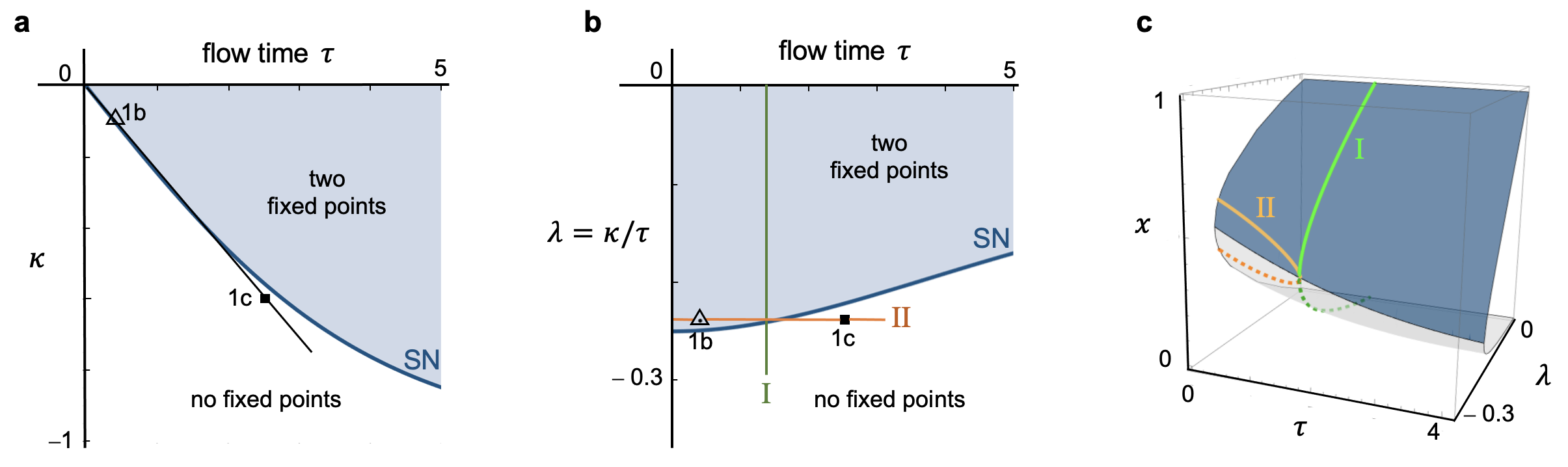
Figure 2: Stability diagram for logistic flow-kick system in parameters flow time $\tau$ and kick $\kappa$ (panel a) or $\tau$ and disturbance rate $\lambda=\kappa/\tau$ (panel b). Marked points correspond to parameter combinations in Figure 1b and 1c. (c) Surface of flow-kick fixed points over $\tau,\lambda$ parameter space.

To better visualize disturbance rates and the connections between ODE and flow-kick systems, we change coordinates in Figure 2b,c to the parameters $\tau$ and $\kappa/\tau\equiv\lambda$. Within this parameter space, flow-kick maps with the same average disturbance rates lie on horizontal lines. We claim that as $\tau$ approaches zero from the right along a line $\lambda=\lambda_{0}$, flow-kick systems with ever higher disturbance frequencies approach the continuous system

$$x^{\prime}=x(1-x)+\lambda_{0}.$$ (5)

We call (5) the continuous limit of the collection of flow-kick maps with average disturbance rate $\lambda_{0}$. Proposition 1 in Section 1 makes this idea precise and generalizes it to a broader class of disturbance functions.

Figure 2b also highlights relationships between bifurcations in the continuously and discretely disturbed logistic system. Given that each point $(\tau,\lambda)=(0,\lambda_{0})$ on the vertical axis in Figure 2b represents—in some sense—an ODE (5), we observe that the curve of flow-kick saddle-node bifurcations (marked SN) emanates from the saddle-node bifurcation at $\lambda=-0.25$ for the continuously disturbed logistic. We prove in Section 4 (Theorem 2) that for $x\in\mathbb{R}$, saddle-node bifurcations continue from ODE to flow-kick systems under modest assumptions. We generalize from the constant disturbance rate $\lambda$ considered here to a parameterized disturbance rate function $r(x,\lambda)$. Theorem 2 connects bifurcations in $\lambda$ of a continuous system to bifurcations in $\lambda$ of a flow-kick systems, shown for the logistic as the green curve (I) in Figure 2c. The logistic example also features a saddle-node bifurcation in $\tau$, shown as the orange curve (II) in Figure 2c. After Theorem 2, we discuss a conjecture that a saddle-node bifurcation in $\lambda$ in a continuous system predicts saddle-node bifurcations in $\tau$ in analogous flow-kick systems.

Although we focus on the saddle-node—the only codimension-1 bifurcation for $x\in\mathbb{R}^{1}$— transcritical bifurcations also commonly arise in ecological models that feature $x=0$ as an extinction equilibrium across parameter values. In Section 4, we show that transcritical bifurcations continue from ODE to flow-kick systems in this setting (Theorem 3).

In summary, the paper is organized as follows. Section 1 establishes definitions and notation. In section 2 we formalize the idea of a continuous limit of flow-kick maps. Sections 3 and 4 treat continuation of fixed points and bifurcations, respectively, from ODE to flow-kick systems. In section 5 we illustrate our results numerically in two models pertaining to vegetation-water and predator-prey dynamics. These examples raise topics for future study such as continuation of Hopf bifurcations, which we discuss in Section 6.

1 Preliminaries and Notation

Flows

Throughout, we consider undisturbed dynamics modeled by an ODE of the form

$$x^{\prime}=f(x)$$ (6)

where $x(t)$ is a function from $\mathbb{R}$ to $\mathbb{R}^{n}$, ^′ denotes $d/dt$, and $f:U\to\mathbb{R}^{n}$ is a $C^{4}$ vector field defined on an open set $U\subseteq\mathbb{R}^{n}$. The vector field $f$ generates a local $C^{4}$ flow function on a subset of $\mathbb{R}\times U$ given by

$$\varphi(t,x_{0})=x(t),$$ (7)

where $x(t)$ is the position of a solution to (6) that starts at $x_{0}$ and flows for time $t$. We will assume that the flow is defined on any time interval of interest. Fixing $t$ yields a time-$t$ map $\varphi_{t}:U\to U$ given by

$$\varphi_{t}(x)=\varphi(t,x).$$ (8)

Given an ODE $x^{\prime}=g(x)$, we will use the terms equilibrium and fixed point interchangeably to describe $x\in\mathbb{R}^{n}$ such that $g(x)=0$.

Kicks

To incorporate disturbances into dynamics, we choose a flow time $t=\tau$, representing the period between disturbances, and add a discrete kick to the time-$\tau$ map.

Definition 1.

A kick is a $C^{1}$ function $k:U\to\mathbb{R}^{n}$.

Definition 2.

For a kick function $k$, the corresponding flow-kick map $\Psi_{\tau,k}:U\to\mathbb{R}^{n}$ is given by

$$\Psi_{\tau,k}(x)=\varphi_{\tau}(x)+k(\varphi_{\tau}(x)).$$

For example, if $k(u)=\kappa$ for a constant $\kappa\in\mathbb{R}^{n}$, then the flow-kick map

$$\Psi_{\tau,k}(x)=\varphi_{\tau}(x)+\kappa$$ (9)

matches the disturbance forms considered in [4]. By choosing $k(u)=-\kappa u$ we obtain the “multiplicative” flow-kick map studied in [5]:

$$\Psi_{\tau,k}(x)=\varphi_{\tau}(x)-\kappa\varphi_{\tau}(x)$$ (10)

Discrete Dynamics

Iterating $\Psi_{\tau,k}$ generates discrete dynamics. We focus the present study on the fixed points of these dynamics, where disturbance and recovery processes balance.

Definition 3.

A flow-kick fixed point is a solution to $\Psi_{\tau,k}(x)=x$, or equivalently
$\varphi_{\tau}(x)+k(\varphi_{\tau}(x))=x$.

It is worth noting that since $\Psi_{\tau,k}$ maps from $U$ to $\mathbb{R}^{n}$, it is possible for a flow-kick trajectory to leave $U$. For example, if $U$ is the interval $(0,\infty)$ in the introductory logistic example, the bottom trajectory in Figure 1b leaves $U$. However, this will not trouble our local study of fixed points in the open set $U$.

Disturbance Coordinates

In the context of the logistic system with constant kicks $\kappa$, Figure 2 summarizes system behavior over two alternative disturbance parameter choices: $(\tau,\kappa)$ in panel (a) and $(\tau,\lambda\equiv\kappa/\tau)$ in panel (b). We generalize the coordinate change between these two panels to non-constant disturbances.

Definition 4.

A disturbance rate function is a $C^{2}$ function $r:U\to\mathbb{R}^{n}$.

A disturbance rate function can be incorporated continuously into an ODE model as $x^{\prime}=f(x)+r(x)$ or used to generate a kick $k(u)=\tau r(u)$ in a flow-kick model.

Definition 5.

The flow-kick map associated with a disturbance rate function $r:U\to\mathbb{R}^{n}$ is

$$\Phi_{\tau,r}(x)=\Psi_{\tau,\tau r}=\varphi_{\tau}(x)+\tau r(\varphi_{\tau}(x)).$$

Henceforth we use the notation of Definition 5 to describe families of flow-kick maps in terms of their disturbance rate functions $r$ and flow times $\tau$. The disturbance rate function $r$ may be omitted from the subscript of $\Phi$ when it is clear from context.

2 Continuous limit of flow-kick systems

The similarities between the continuous harvest model (Figure 1a) and the flow-kick harvest model (Figure 1b) reflect a broader phenomenon: flow-kick maps generate an analogous vector field in the limit as flow times go to zero and the disturbance rate is maintained. This result has been shown for specific flow-kick maps in [4, 6]. Here we state and prove a more general formulation using the current notation.

Proposition 1.

Let $f(x)$ be a vector field governing undisturbed dynamics and $r(x)$ be a disturbance rate function. In the limit as $\tau\to 0$, the family of flow-kick maps $\Phi_{\tau,r}(x)=\varphi_{\tau}(x)+\tau r(\varphi_{\tau}(x))$ generates the vector field $f(x)+r(x)$.

Proof: To calculate the vector field generated by $\Phi_{\tau,r}$ as $\tau\to 0$ we use the derivative of this time-dependent mapping with respect to $\tau$ at $\tau=0$. Note that $\Phi_{0,r}(x)$ is the identity; that is, $\Phi_{0,r}(x)=x$. We have

$$\lim\limits_{\tau\to 0}\frac{\Phi_{\tau,r}(x)-x}{\tau} =\lim\limits_{\tau\to 0}\frac{\varphi_{\tau}(x)+\tau r(\varphi_{\tau}(x))-x}{\tau}.$$ (11)

Because the flow function $\varphi$ is twice differentiable, it can be expanded in the time variable via Taylor’s formula as

$$\varphi(\tau,x) =\varphi(0,x)+\tau\frac{\partial\varphi}{\partial t}(0,x)+O(\tau^{2})$$ (12)

$$=x+\tau f(x)+O(\tau^{2}).$$

Here we have employed Landau big-O notation in a neighborhood of $\tau=0$. Substituting (12) into (11) and simplifying yields

$$\lim\limits_{\tau\to 0}\frac{\Phi_{\tau,r}(x)-x}{\tau} =\lim\limits_{\tau\to 0}\frac{\tau f(x)+\tau r(\varphi_{\tau}(x))+O(\tau^{2})}{\tau}$$ (13)

$$=\lim\limits_{\tau\to 0}\big{(}f(x)+r(\varphi_{\tau}(x))+O(\tau)\big{)}$$

$$=f(x)+r(x),$$

as claimed. ∎

We can visualize Proposition 1 for the harvested logistic example in Figure 2, where the disturbance rate function is a constant $r(x)=\lambda$. Each value of $\lambda=\kappa/\tau$ yields a line with slope $\lambda$ through the origin in Figure 2a. In Figure 2b, fixing $\lambda=0.24$ yields a horizontal line. Proposition 1 concerns the limit of the flow-kick maps parameterized along these lines as $\tau\to 0^{+}$. Note that limits along different lines generate different continuous systems $x^{\prime}=f(x)+\lambda$. In this sense the origin in Figure 2a and the vertical axis in Figure 2b each represent a continuum of vector fields that result from taking $\tau$ to $0$ with different disturbance rates $\lambda$. On the other hand, the literal flow-kick map parameterized by $\tau=0$ is the identity map, as $\Phi_{0,r}(x)=\varphi_{0}(x)+0r(\varphi_{0}(x))=x$.

3 Continuation of equilibria to fixed points

Under suitable nondegeneracy conditions, an equilibrium for continuous disturbance continues locally to a flow-kick fixed point when we discretize the disturbance, maintaining the same average rate:

Proposition 2.

If $x_{*}\in U$ is an equilibrium for the continuous system $x^{\prime}=f(x)+r(x)$ and
$D_{x}[f+r](x_{*})$ is invertible, then $x_{*}$ continues locally to flow-kick fixed points. That is, there exists $\delta>0$ and a family $\{x_{\tau}\}_{\tau\in[0,\delta)}\subset U$ satisfying

1. each $x_{\tau}$ is a fixed point for the flow-kick map $\Phi_{\tau,r}(x)=\varphi_{\tau}(x)+\tau r(\varphi_{\tau}(x))$,

2. the flow-kick fixed points $x_{\tau}$ vary continuously as a function of $\tau$, and

3. the branch of flow-kick fixed points emerges from the equilibrium $x_{*}$; that is, $x_{0}=x_{*}$.

Proof: Flow-kick fixed points $x\in U$ are those that satisfy $\Phi_{\tau,r}(x)=x$, or equivalently

$$\varphi_{\tau}(x)+\tau r(\varphi_{\tau}(x))-x=0.$$ (14)

When $\tau=0$, all points $x\in U$ satisfy equation (14). To remove this degeneracy and connect to $x_{*}$ we expand $\varphi$ in $t$ about 0:

$$\varphi_{\tau}(x)=\varphi(\tau,x) =\varphi(0,x)+\tau\frac{\partial\varphi}{\partial t}(0,x)+\tau^{2}\int_{0}^{1}(1-u)\frac{\partial^{2}\varphi}{\partial t^{2}}(u\tau,x)du$$ (15)

$$=x+\tau f(x)+\tau^{2}\int_{0}^{1}(1-u)\frac{\partial^{2}\varphi}{\partial t^{2}}(u\tau,x)du.$$ (16)

In (15) we have employed an integral form of the remainder articulated by Folland [17] and derived in Appendix A. Substituting (16) into (14) and simplifying yields

$$\tau\left(f(x)+r(\varphi_{\tau}(x))+\tau\int_{0}^{1}(1-u)\frac{\partial^{2}\varphi}{\partial t^{2}}(u\tau,x)du\right)=0.$$ (17)

To solve (14) it suffices to find zeros of the second factor in (17). We do this via the Implicit Function Theorem applied to the function $F:\mathbb{R}\times U\to\mathbb{R}^{n}$ given by

$$F(\tau,x)=f(x)+r(\varphi_{\tau}(x))+\tau\int_{0}^{1}(1-u)\frac{\partial^{2}\varphi}{\partial t^{2}}(u\tau,x)du.$$ (18)

Given the smoothness assumptions on $f$, $r$, and $\varphi$, one can confirm from (18) that $F$ is $C^{1}$. Further, $F(0,x_{*})=f(x_{*})+r(x_{*})=0$, since $x_{*}$ is a fixed point for the continuous system. Lastly, we have that

$$D_{x}F(0,x_{*}) =D_{x}\left.[f(x)+r(\varphi_{0}(x))]\right|_{x=x_{*}}$$ (19)

$$=D_{x}[f+r](x_{*})$$ (20)

is invertible, by hypothesis. It follows from the Implicit Function Theorem that for some $\delta>0$, there exists a $C^{1}$ function $g:[0,\delta)\to U$ satisfying $g(0)=x_{*}$ and $F(\tau,g(\tau))=0$. Letting $x_{\tau}=g(\tau)$, the proposition follows.∎

With slightly stronger hypotheses on the spectrum of $D_{x}[f+r](x_{*})$, the stability of continuous-disturbance fixed point $x_{*}$ persists locally along the branch $x_{\tau}$ of flow-kick fixed points:

Theorem 1.

If $x_{*}\in U$ is a hyperbolic equilibrium of the continuous system $x^{\prime}=f(x)+r(x)$ and $\tau>0$ is sufficiently small, then flow-kick fixed points $x_{\tau}$ not only continue from $x_{*}$ as in Proposition 2 but also inherit the stability of $x_{*}$.

Proof: Consider a fixed point $x_{*}$ of $x^{\prime}=f(x)+r(x)$ that is hyperbolic, meaning all eigenvalues of $D_{x}[f+r](x_{*})$ have nonzero real part. By Proposition 2, a continuous family of flow-kick fixed points $\{x_{\tau}\}_{\tau\in[0,\delta)}$ emanates locally in $\tau$ from $x_{0}=x_{*}$. We classify the stability of a fixed point $x_{\tau}$ using the Jacobian matrix

$$D_{x}\Phi_{\tau,r}(x) =D_{x}[\varphi_{\tau}(x)+\tau r(\varphi_{\tau}(x))]$$

$$=D_{x}\left[x+\tau f(x)+\tau^{2}\int_{0}^{1}(1-u)\frac{\partial^{2}\varphi}{\partial t^{2}}(u\tau,x)du\right]+D_{x}\Big{[}\tau r(\varphi_{\tau}(x))\Big{]}$$

$$=I+\tau\left[D_{x}f(x)+D_{x}r(\varphi_{\tau}(x))+\tau D_{x}\int_{0}^{1}(1-u)\frac{\partial^{2}\varphi}{\partial t^{2}}(u\tau,x)du\right]$$

$$=I+\tau A(\tau,x)$$

where $A$ is the matrix-valued function

$$A(\tau,x)=D_{x}f(x)+D_{x}r(\varphi_{\tau}(x))+\tau D_{x}\displaystyle\int_{0}^{1}(1-u)\frac{\partial^{2}\varphi}{\partial t^{2}}(u\tau,x)du.$$

Let $\lambda_{1}(\tau),\dots,\lambda_{n}(\tau)$ be the eigenvalues of $A(\tau,x_{\tau})$, counted with multiplicities. Let $a_{i}(\tau)$ and $b_{i}(\tau)$ denote the real and imaginary parts of $\lambda_{i}(\tau)$, respectively. The hyperbolicity of $x_{*}$ implies that each eigenvalue $\lambda_{i}(0)$ of $A(0,x_{0})=D_{x}f(x_{*})+D_{x}r(x_{*})$ has $a_{i}(0)\not=0$. Furthermore, $f$, $r$, $\varphi$, and $x_{\tau}$ are sufficiently smooth so that the function $A(\tau,x_{\tau})$ varies continuously in $\tau$ along the branch of flow-kick fixed points. It follows from continuity of eigenvalues with respect to matrix perturbations (see, e.g. [18]) that for some $\delta_{1}\in(0,\delta]$, $0\leq\tau<\delta_{1}$ ensures $\text{sign}(a_{i}(\tau))=\text{sign}(a_{i}(0))$ for $i=1,\dots,n$. In other words, $\delta_{1}$ bounds the neighborhood in which the eigenvalues of $A$ do not cross the imaginary axis.

One may confirm via characteristic equations that the eigenvalues $\mu_{1}(\tau),\dots,\mu_{n}(\tau)$ of the derivative matrix $D_{x}\Phi_{\tau}(x_{\tau})$ are related to the eigenvalues of $A(\tau,x_{\tau})$ by

$$\mu_{i}(\tau)=1+\tau\lambda_{i}(\tau).$$ (21)

Stability of the flow-kick fixed point $x_{\tau}$ depends on size of the moduli

$$|\mu_{i}(\tau)|=|1+\tau(a_{i}(\tau)+b_{i}(\tau)i)|=\sqrt{1+\tau(2a_{i}(\tau)+\tau(a_{i}(\tau)^{2}+b_{i}(\tau)^{2}))}$$ (22)

relative to 1. Recall flow-kick fixed points correspond to $\tau>0$. In the case that $a_{i}(0)>0$, then for $0<\tau<\delta_{1}$, we have $a_{i}(\tau)>0$, and it follows readily that $|\mu_{i}(\tau)|>1$. If instead $a_{i}(0)<0$, then for $0<\tau<\delta_{1}$, we have $a_{i}(\tau)<0$. Note that the factor $2a_{i}(\tau)+\tau(a_{i}(\tau)^{2}+b_{i}(\tau)^{2})$ in (22) is a continuous function of $\tau$ that evaluates to $2a_{i}(0)<0$ when $\tau=0$. Thus there exists a $\delta_{2}>0$ such that $2a_{i}(\tau)+\tau(a_{i}(\tau)^{2}+b_{i}(\tau)^{2})<0$ whenever $0<\tau<\delta_{2}$. Taking $\delta_{3}=\min(\delta_{1},\delta_{2})$ ensures that $|\mu_{i}(\tau)|<1$ whenever $a_{i}(\tau)<0$ and $0<\tau<\delta_{3}$.

In this way stable and unstable eigenvalues $\lambda_{i}(0)$ of the vector field $f(x)+r(x)$ at $x_{*}$ continue locally to stable and unstable, respectively, eigenvalues $\mu_{i}(\tau)$ of the flow-kick map $\Phi_{\tau,r}$ at $x_{\tau}$. ∎

.

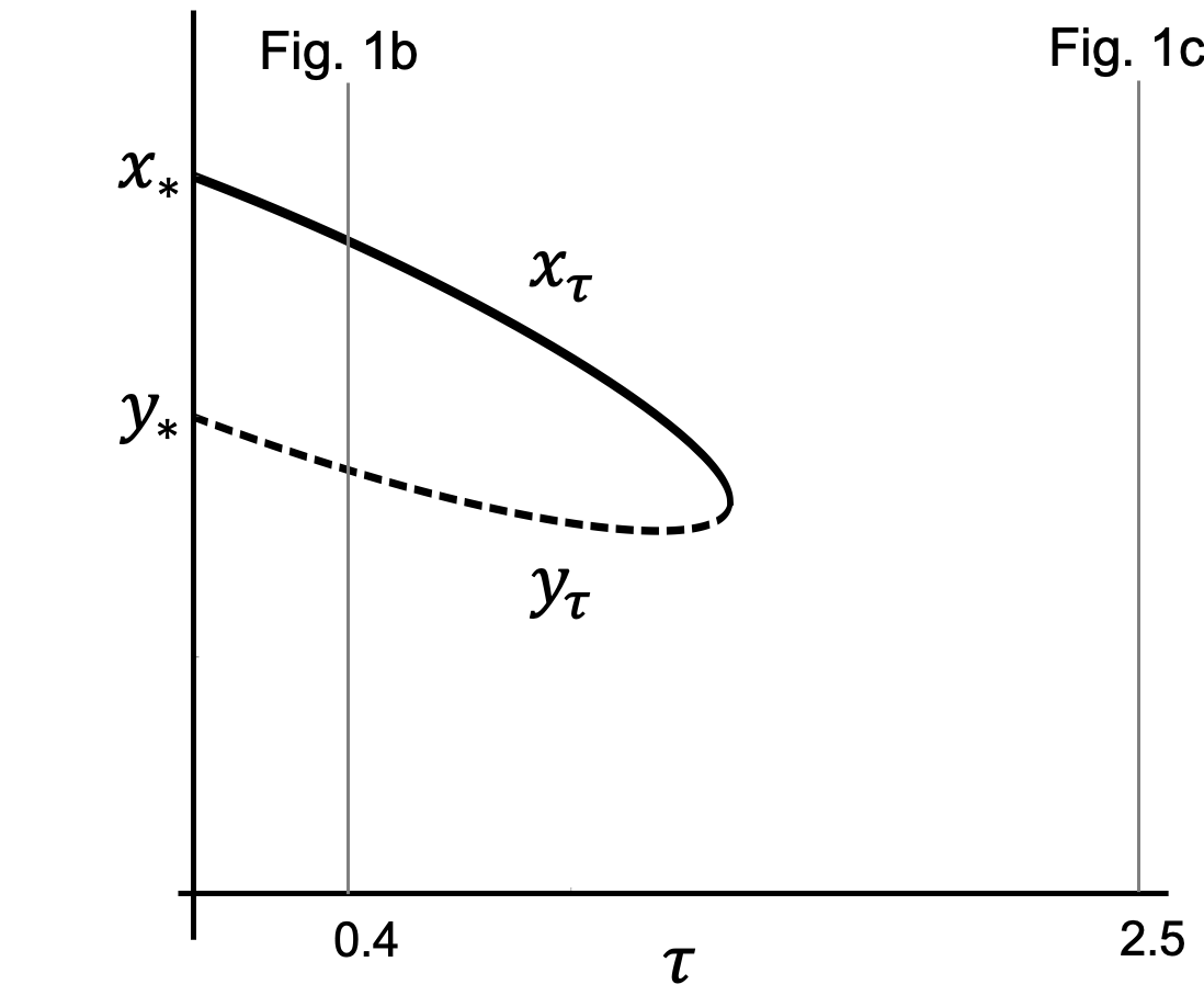
Figure 3: Logistic flow-kick fixed points with $r(u)=-0.24$

To connect the notation of Theorem 1 to the introductory logistic example, consider logistic growth generated by

$$x^{\prime}=f(x)=x(1-x)$$

with disturbance rate $r(x)=-0.24$. Figure 3 illustrates the branches $x_{\tau}$ (stable) and $y_{\tau}$ (unstable) of flow-kick fixed points that continue from the ODE equilibria $x_{*}$ and $y_{*}$ shown in Figure 1a. Vertical lines mark the values of $\tau$ used for flow-kick systems in Figure 1b and 1c. Near $\tau=1.4$ the branches meet in a saddle-node bifurcation—the same one illustrated by curve (II) in Figure 2c. We turn to bifurcation continuation in Section 4.

4 Continuation of bifurcations

As bifurcations in flow-kick systems represent qualitative shifts in dynamics brought about by small changes in disturbance patterns, they can help predict tipping and regime changes in ecological and other systems. To study bifurcations in a disturbance parameter $\lambda\in\mathbb{R}$, we augment the domain of our disturbance rate function $r$.

Definition 6.

A parameterized disturbance rate function is a function $r(u;\lambda)$ from $U\times\mathbb{R}$ to $\mathbb{R}^{n}$.

We restrict to $n=1$ ($x\in\mathbb{R}$) and study the connections between bifurcations in the ODE system

$$x^{\prime}=f(x)+r(x;\lambda)$$

and those of the flow-kick map

$$\Phi_{\tau}(x;\lambda)=\varphi_{\tau}(x)+\tau r(\varphi_{\tau}(x);\lambda).$$

We will denote the first argument of $r$ as $x$ in the continuous context and as $u$ in the flow-kick context; the latter is for ease of tracking composition of $r$ with $\varphi$. We first treat saddle-node bifurcations, then transcritical. In sections 5 and 6 we consider extensions to higher dimensional systems—including Hopf bifurcations—in the context of climate and predator-prey examples.

Saddle-node bifurcations

We use Wiggins’ characterizations [19] as our definitions of saddle-node bifurcations in the parameter $\lambda$ for the vector field $f(x)+r(x;\lambda)$ and the flow-kick map $\Phi_{\tau}(x;\lambda)$. Table 1 provides the four defining conditions for each system. With mild smoothness assumptions on the disturbance rate function $r$, saddle-node bifurcations continue locally from the ODE to flow-kick systems.

	Vector field $f(x)+r(x;\lambda)$	Map $\Phi_{\tau}(x;\lambda)$
Saddle-Node Bifurcation at	$(x_{*};\lambda_{*})$	$(x_{\tau};\lambda_{\tau})$
Fixed Point	$f(x_{*})+r(x_{*};\lambda_{*})=0$	$\Phi_{\tau}(x_{\tau};\lambda_{\tau})=x_{\tau}$
Nonhyperbolic	$\frac{\partial f}{\partial x}(x_{*})+\frac{\partial r}{\partial x}(x_{*};\lambda_{*})=0$	$\frac{\partial\Phi_{\tau}}{\partial x}(x_{\tau};\lambda_{\tau})=1$
Transversality	$\frac{\partial f}{\partial\lambda}(x_{*})+\frac{\partial r}{\partial\lambda}(x_{*};\lambda_{*})\not=0$	$\frac{\partial\Phi_{\tau}}{\partial\lambda}(x_{\tau};\lambda_{\tau})\not=0$
Quadratic Dominance	$\frac{\partial^{2}f}{\partial x^{2}}(x_{*})+\frac{\partial^{2}r}{\partial x^{2}}(x_{*};\lambda_{*})\not=0$	$\frac{\partial^{2}\Phi_{\tau}}{\partial x^{2}}(x_{\tau};\lambda_{\tau})\not=0$

Table 1: Saddle-node bifurcation conditions [19].

Theorem 2.

Let $r(u;\lambda)$ be $C^{2}$. If the 1D system $x^{\prime}=f(x)+r(x;\lambda)$ undergoes a saddle-node bifurcation in the parameter $\lambda$ at $(x_{*};\lambda_{*})$, then for sufficiently small $\tau>0$ there exists a branch $(x_{\tau};\lambda_{\tau})$ of saddle-node bifurcations in $\lambda$ for the flow-kick maps $\Phi_{\tau}(x;\lambda)=\varphi_{\tau}(x)+\tau r(\varphi_{\tau}(x);\lambda)$ that varies continuously in $\tau$ and limits to $(x_{*};\lambda_{*})$ as $\tau\to 0$.

Proof: We will first show that a nonhyperbolic fixed point for the vector field $f(x)+r(x;\lambda)$ continues to a branch of nonhyperbolic fixed points for the flow-kick maps $\Phi_{\tau}(x;\lambda)$, and then confirm that the transversality and quadratic dominance conditions persist locally along this branch.

Consider the mapping $\tilde{F}:\mathbb{R}\times U\times\mathbb{R}\to\mathbb{R}^{2}$ given by

$$\tilde{F}(\tau,x,\lambda)=\begin{bmatrix}\Phi_{\tau}(x;\lambda)-x\\ \frac{\partial}{\partial x}\Phi_{\tau}(x;\lambda)-1\end{bmatrix}.$$ (23)

Zeros of $\tilde{F}$ correspond to nonhyperbolic fixed points $x$ of the flow-kick map. But for $\tau=0$, all choices of $x$ and $\lambda$ yield zeros of $\tilde{F}$. To eliminate this degeneracy, we manipulate $\tilde{F}$. Using the Taylor expansion of the flow $\varphi$ in time about $\tau=0$ and Folland’s integral form of the remainder [17] as in the proof of Proposition 2, we obtain

$$\tilde{F}(\tau,x,\lambda)=\tau\begin{bmatrix}f(x)+r(\varphi_{\tau}(x);\lambda)+\tau\displaystyle\int_{0}^{1}(1-s)\dfrac{\partial^{2}\varphi}{\partial t^{2}}(s\tau,x)ds\\ \dfrac{df}{dx}(x)+\dfrac{\partial r}{\partial u}(\varphi_{\tau}(x);\lambda)\dfrac{\partial\varphi}{\partial x}(\tau,x)+\tau\displaystyle\int_{0}^{1}(1-s)\dfrac{\partial^{3}\varphi}{\partial x\partial t^{2}}(s\tau,x)ds\end{bmatrix}\equiv\tau F(\tau,x,r).$$ (24)

Here we have defined the mapping $F:\mathbb{R}\times U\times\mathbb{R}\to\mathbb{R}^{2}$ to exclude a factor of $\tau$ from $\tilde{F}$; we note that the zeros of $F$ also give nonhyperbolic flow-kick fixed points.

One may confirm that $F$ is $C^{1}$ using the smoothness of $f$, $r$, and $\varphi$. From our hypothesis that $(x_{*};\lambda_{*})$ gives a nonhyperbolic fixed point in the continuous system $x^{\prime}=f(x)+r(x;\lambda)$, we also have

$$F(0,x_{*},\lambda_{*})=\begin{bmatrix}f(x_{*})+r(\varphi_{0}(x_{*});\lambda_{*})\\ \dfrac{\partial f}{\partial x}(x_{*})+\dfrac{\partial r}{\partial u}(\varphi_{0}(x_{*});\lambda_{*})\dfrac{\partial\varphi}{\partial x}(0,x_{*})\end{bmatrix}=\begin{bmatrix}f(x_{*})+r(x_{*};\lambda_{*})\\ \dfrac{\partial f}{\partial x}(x_{*})+\dfrac{\partial r}{\partial x}(x_{*};\lambda_{*})\end{bmatrix}=\begin{bmatrix}0\\ 0\end{bmatrix}.$$ (25)

In the second equation of (25) we have used the fact that the spatial derivative of the flow at time zero is one and changed variables from $u$ to $x$ for the first argument to the disturbance rate function. Before applying the Implicit Function Theorem to $F$, we check its matrix of derivatives in $x$ and $\lambda$ for invertibility at $(\tau,x,\lambda)=(0,x_{*},\lambda_{*})$. We have

$$D_{x,\lambda}F=\begin{bmatrix}\dfrac{\partial f}{\partial x}+\dfrac{\partial r}{\partial u}\dfrac{\partial\varphi}{\partial x}+\tau\displaystyle\int_{0}^{1}(1-s)\dfrac{\partial^{3}\varphi}{\partial x\partial t^{2}}(s\tau,x)ds&&&\dfrac{\partial r}{\partial\lambda}\vspace{0.2cm}\\ \dfrac{\partial^{2}f}{\partial x^{2}}+\dfrac{\partial r}{\partial u}\dfrac{\partial^{2}\varphi}{\partial x^{2}}+\dfrac{\partial^{2}r}{\partial u^{2}}\left(\dfrac{\partial\varphi}{\partial x}\right)^{2}+\tau\displaystyle\int_{0}^{1}(1-s)\dfrac{\partial^{4}\varphi}{\partial x^{2}\partial t^{2}}(s\tau,x)ds&&&\dfrac{\partial^{2}r}{\partial\lambda\partial u}\dfrac{\partial\varphi}{\partial x}\end{bmatrix}.$$ (26)

Evaluating (26) at $(\tau,x,\lambda)=(0,x_{*},\lambda_{*})$ and using the facts $\dfrac{\partial\varphi}{\partial x}(0,x)=1$ and $\dfrac{\partial^{2}\varphi}{\partial x^{2}}(0,x)=0$ yields

$$D_{x,\lambda}F(0,x_{*},\lambda_{*})=\begin{bmatrix}\dfrac{\partial f}{\partial x}(x_{*})+\dfrac{\partial r}{\partial u}(x_{*},\lambda_{*})&&&\dfrac{\partial r}{\partial\lambda}(x_{*};\lambda_{*})\vspace{0.2cm}\\ \dfrac{\partial^{2}f}{\partial x^{2}}(x_{*})+\dfrac{\partial^{2}r}{\partial u^{2}}(x_{*};\lambda_{*})&&&\dfrac{\partial^{2}r}{\partial\lambda\partial u}(x_{*},\lambda_{*})\end{bmatrix}.$$ (27)

The top left entry of (27) is zero due to the continuous system’s nonhyperbolic condition. The bottom left entry of (27) is nonzero by quadratic dominance in the continuous system. The top right entry is nonzero because transversality in the continuous system gives $\frac{\partial f}{\partial\lambda}(x_{*})+\frac{\partial r}{\partial\lambda}(x_{*},\lambda_{*})\not=0$ and $\frac{\partial f}{\partial\lambda}(x_{*})=0$. It follows that the matrix in $\eqref{eq:DF3}$ is invertible.

The Implicit Function Theorem then implies that there exists $\delta>0$ and a $C^{1}$ function $g:[0,\delta)\to U\times\mathbb{R}$, $g(\tau)=(x_{\tau};\lambda_{\tau})$, such that $g(0)=(x_{*};\lambda_{*})$ and $F(\tau,x_{\tau},\lambda_{\tau})=0$ for all $\tau\in[0,\delta)$. Note that in this parameterization, at $\tau=0$ we have the bifurcation point from the continuous system; i.e. $(x_{0};\lambda_{0})=(x_{*};\lambda_{*})$. Continuity of $g$ implies $(x_{\tau},\lambda_{\tau})\to(x_{*},\lambda_{*})$ as $\tau\to 0$. The pairs $(x_{\tau};\lambda_{\tau})$ give the desired branch of nonhyperbolic fixed points $x_{\tau}$ for the flow-kick maps $\Phi_{\tau}(x;\lambda_{\tau})$.

These nonhyperbolic fixed points are candidates for saddle-node bifurcation points, as they the satisfy the first two conditions in Table 1. Next we confirm transversality in $\lambda$ and quadratic dominance in $x$ along the branch $\{(x_{\tau};\lambda_{\tau})\}$ for sufficiently small $\tau>0$. Collectively the four conditions show that a saddle-node bifurcation occurs in $\lambda$ at $x_{\tau}$.

Towards transversality, note that for $\Phi_{\tau}(x;\lambda)=\varphi_{\tau}(x)+\tau r(\varphi_{\tau}(x);\lambda)$, we get

$$\frac{\partial\Phi_{\tau}}{\partial\lambda}(x_{\tau},\lambda_{\tau})=\tau\frac{\partial r}{\partial\lambda}(\varphi_{\tau}(x_{\tau}),\lambda_{\tau}).$$ (28)

The factor $\frac{\partial r}{\partial\lambda}(\varphi_{\tau}(x_{\tau}),\lambda_{\tau})$ in (28) is a continuous function of $\tau$ on the interval $[0,\delta)$. At $\tau=0$ it takes the value

$$\frac{\partial r}{\partial\lambda}(\varphi_{0}(x_{0}),\lambda_{0})=\frac{\partial r}{\partial\lambda}(x_{*},\lambda_{*}),$$ (29)

which must be nonzero because transversality in the continuous system gives $\frac{\partial f}{\partial\lambda}(x_{*})+\frac{\partial r}{\partial\lambda}(x_{*};\lambda_{*})\not=0$ but $\frac{\partial f}{\partial\lambda}=0$. By continuity, $\frac{\partial r}{\partial\lambda}(x_{\tau},\lambda_{\tau})$ remains nonzero for $\tau$ in some interval $(0,\delta_{1})$, where $0<\delta_{1}\leq\delta$. As a result, $\frac{\partial\Phi_{\tau}}{\partial\lambda}(x_{\tau},\lambda_{\tau})$ is nonzero on the interval $(0,\delta_{1})$, and transversality in the flow-kick system holds on this interval.

To verify quadratic dominance, we compute

$$\frac{\partial^{2}\Phi_{\tau}}{\partial x^{2}}(x,\lambda) =\frac{\partial^{2}}{\partial x^{2}}\left[\varphi(\tau,x)+\tau r(\varphi(\tau,x),\lambda)\right]$$ (30)

$$=\frac{\partial}{\partial x}\left[\frac{\partial\varphi}{\partial x}(\tau,x)+\tau\frac{\partial r}{\partial u}(\varphi(\tau,x),\lambda)\frac{\partial\varphi}{\partial x}(\tau,x)\right]$$ (31)

$$=\frac{\partial^{2}\varphi}{\partial x^{2}}(\tau,x)+\tau\frac{\partial^{2}r}{\partial u^{2}}(\varphi(\tau,x),\lambda)\left(\frac{\partial\varphi}{\partial x}(\tau,x)\right)^{2}+\tau\frac{\partial r}{\partial u}(\varphi(\tau,x),\lambda)\frac{\partial^{2}\varphi}{\partial x^{2}}(\tau,x).$$ (32)

Now

$$\frac{\partial^{2}\varphi}{\partial x^{2}}(\tau,x) =\frac{\partial^{2}}{\partial x^{2}}\left[x+\tau f(x)+\tau^{2}\int_{0}^{1}(1-s)\frac{\partial^{2}\varphi}{\partial t^{2}}(s\tau,x)ds\right]$$ (33)

$$=\tau\frac{d^{2}f}{dx^{2}}(x)+\tau^{2}\int_{0}^{1}(1-s)\frac{\partial^{4}\varphi}{\partial x^{2}\partial t^{2}}(s\tau,x)ds.$$ (34)

Replacing $\frac{\partial^{2}\varphi}{\partial x^{2}}$ with (34) in equation (32) and rearranging, we get

$$\frac{\partial^{2}\Phi_{\tau}}{\partial x^{2}}(\tau,x) =\tau\Bigg{(}\frac{d^{2}f}{dx^{2}}(x)+\frac{\partial^{2}r}{\partial u^{2}}(\varphi(\tau,x),\lambda)\left(\frac{\partial\varphi}{\partial x}(\tau,x)\right)^{2}+\tau\int_{0}^{1}(1-s)\frac{\partial^{4}\varphi}{\partial x^{2}\partial t^{2}}(s\tau,x)ds$$ (35)

$$\hskip 128.0374pt+\frac{\partial r}{\partial u}\left(\tau\frac{d^{2}f}{dx^{2}}(x)+\tau^{2}\int_{0}^{1}(1-s)\frac{\partial^{4}\varphi}{\partial x^{2}\partial t^{2}}(s\tau,x)ds\right)\Bigg{)}$$

Clearly the first factor of (35) is nonzero for $\tau>0$. We evaluate the second factor in (35) at $(x_{\tau},\lambda_{\tau})$ to define the continuous function $h:[0,\delta)\to\mathbb{R}$ as

$$h(\tau) =\frac{d^{2}f}{dx^{2}}(x_{\tau})+\frac{\partial^{2}r}{\partial u^{2}}(\varphi(\tau,x_{\tau}),\lambda_{\tau})\left(\frac{\partial\varphi}{\partial x}(\tau,x_{\tau})\right)^{2}+\tau\int_{0}^{1}(1-s)\frac{\partial^{4}\varphi}{\partial x^{2}\partial t^{2}}(s\tau,x_{\tau})ds$$ (36)

$$\hskip 128.0374pt+\frac{\partial r}{\partial u}\left(\tau\frac{d^{2}f}{dx^{2}}(x_{\tau})+\tau^{2}\int_{0}^{1}(1-s)\frac{\partial^{4}\varphi}{\partial x^{2}\partial t^{2}}(s\tau,x_{\tau})ds\right).$$

We have that

$$h(0)=\frac{d^{2}f}{dx^{2}}(x_{0})+\frac{\partial^{2}r}{\partial u^{2}}(\varphi(0,x_{0}),\lambda_{0})\left(\frac{\partial\varphi}{\partial x}(0,x_{0})\right)^{2}=\frac{d^{2}f}{dx^{2}}(x_{*})+\frac{\partial^{2}r}{\partial x^{2}}(x_{*},\lambda_{*})$$ (37)

It follows from (37) and quadratic dominance in the continuous system that $h(0)\not=0$. Since $h$ is continuous, there exists a $\delta_{2}\in(0,\delta)$ such that whenever $\tau\in(0,\delta_{2})$ we have $h(\tau)\not=0$ and consequently $\frac{\partial^{2}\Phi_{\tau}}{\partial x^{2}}(x_{\tau},\lambda_{\tau})\not=0$.

Let $\delta_{3}=\min(\delta_{1},\delta_{2})$. For $0<\tau<\delta_{3}$, both transversality and quadratic dominance conditions for saddle-node bifurcations hold along the nonhyperbolic branch of flow-kick fixed points, and the proof is complete. ∎

Theorem 2 concerns bifurcations in the parameter $\lambda$. However, we also saw a saddle-node bifurcation in $\tau$ for the logistic system in Figure 2c and Figure 3, with $\lambda=-0.24$ fixed. One can interpret this bifurcation in $\tau$ as a sign that discrete harvests that were sustainable at high frequencies become unsustainable at lower frequencies, despite maintaining the same average harvest rate.

We conjecture that saddle-node bifurcations in $\lambda$ for an ODE system $x^{\prime}=f(x)+r(x,\lambda)$ continue—under appropriate conditions—to saddle-node bifurcations in $\tau$ for nearby flow-kick systems. To prove this conjecture, one can modify the transversality condition in the argument for Theorem 2, instead requiring that the $\tau$-derivative $\frac{\partial\Phi_{\tau}}{\partial\tau}(x_{\tau};\lambda_{\tau})$ is nonzero. A general result currently eludes us.

Transcritical bifurcations

Since transcritical bifurcations are not generic, we expect that additional conditions are necessary to ensure a transcritical bifurcation continues from ODE to flow-kick systems. In population modeling, a natural condition to consider is a factor of $x$ in the vector field $f(x)+r(x;\lambda)$. This makes $x=0$ (population extinction) an equilibrium across parameter values $\lambda$. In this context, Table 2 displays conditions that define a transcritical bifurcation in the continuous and flow-kick systems [19].

Theorem 3.

Consider a vector field function $f(x)=x\,g(x)$ where $g$ is $C^{4}$ and a disturbance rate function $r(u;\lambda)=u\,s(u;\lambda)$ where $s$ is $C^{1}$. If a transcritical bifurcation at $(x,\lambda)=(0,\lambda_{*})$ occurs in the ODE system $x^{\prime}=x\,g(x)+x\,s(x;\lambda)$, then it continues locally to a branch of transcritical bifurcations in $\lambda$ at $(x,\lambda)=(0,\lambda_{\tau})$ for the flow-kick maps $\Phi_{\tau}(x)=\varphi_{\tau}(x)+\tau\,\varphi_{\tau}(x)\,s(\varphi_{\tau}(x);\lambda)$.

Proof: We follow a modified strategy to the proof of Theorem 2. We do not need the Implicit Function Theorem to extend the fixed point condition (i) in Table 2 from the continuous to the discrete setting because $x=0$ is both an equilibrium for $x^{\prime}=x\,g(x)+x\,s(x;\lambda)$ and a fixed point for $\Phi_{\tau}(x)=\varphi_{\tau}(x)+\tau\varphi_{\tau}(x)\,s(\varphi_{\tau}(x);\lambda)$, regardless of the values of $\lambda$ and $\tau$.

	Vector field	Map $\Phi_{\tau}(x;\lambda)=$
	$x\,g(x)+x\,s(x;\lambda)$	$\varphi_{\tau}(x)+\tau\,\varphi_{\tau}(x)\,s(\varphi_{\tau}(x);\lambda)$
Transcritical Bifurcation at	$(x_{*};\lambda_{*})$	$(x_{\tau};\lambda_{\tau})$
(i) Fixed point	$x_{*}\,g(x_{*})+x_{*}\,s(x_{*};\lambda_{*})=0$	$\Phi_{\tau}(x_{\tau};\lambda_{\tau})=x_{\tau}$
(ii) Nonhyperbolic	$\left.\frac{\partial}{\partial x}[x\,g(x)+x\,s(x;\lambda)]\right|_{(x_{*};\lambda_{*})}=0$	$\frac{\partial\Phi_{\tau}}{\partial x}(x_{\tau};\lambda_{\tau})=1$
(iii) Not transverse	$\left.\frac{\partial}{\partial\lambda}[x\,g(x)+x\,s(x;\lambda)]\right|_{(x_{*};\lambda_{*})}=0$	$\frac{\partial\Phi_{\tau}}{\partial\lambda}(x_{\tau};\lambda_{\tau})=0$
(iv) Mixed partials	$\frac{\partial^{2}}{\partial x\partial\lambda}\left.\left[x\,g(x)+x\,s(x;\lambda)\right]\right|_{(x_{*};\lambda_{*})}\not=0$	$\frac{\partial^{2}\Phi_{\tau}}{\partial x\partial\lambda}(x_{\tau};\lambda_{\tau})\not=0$
(v) Quadratic dominance	$\frac{\partial^{2}}{\partial x^{2}}\left.\left[x\,g(x)+x\,s(x;\lambda)\right]\right|_{(x_{*};\lambda_{*})}\not=0$	$\frac{\partial^{2}\Phi_{\tau}}{\partial x^{2}}(x_{\tau};\lambda_{\tau})\not=0$

Table 2: Transcritical bifurcation conditions [19].

Instead, we restrict to $x=0$ in $(\tau,x,\lambda)$ space and use the Implicit Function Theorem to construct a branch of parameter values $\lambda_{\tau}$ along which the flow-kick map is nonhyperbolic. The nonhyperbolic condition

$$\frac{\partial\Phi_{\tau}}{\partial x}\Big{|}_{x=0}=1$$ (38)

for the flow-kick map is equivalent to

$$\frac{\partial}{\partial x}\Big{[}\varphi_{\tau}(x)+\tau\varphi_{\tau}(x)\,s(\varphi_{\tau}(x);\lambda)\Big{]}\Big{|}_{x=0}-1=0.$$ (39)

Let the function $\tilde{F}(\tau,\lambda)$ take values given by the left side of equation (39), so that zeros of $\tilde{F}$ correspond to combinations of $\tau$ and $\lambda$ that make the flow-kick fixed point $x=0$ nonhyperbolic. Expanding $\varphi_{\tau}(x)$ in $\tau$ and manipulating derivatives, we have

$$\begin{split}\tilde{F}(\tau,\lambda)&=\frac{\partial}{\partial x}\Big{[}x+\tau x\,g(x)+\tau^{2}\int_{0}^{1}(1-v)\frac{\partial^{2}\varphi}{\partial t^{2}}(v\tau,x)dv\Big{]}\Big{|}_{x=0}\\ &\hskip 170.71652pt+\frac{\partial}{\partial x}\Big{[}\tau\varphi_{\tau}(x)\,s(\varphi_{\tau}(x);\lambda)\Big{]}\Big{|}_{x=0}-1\end{split}$$ (40)

$$\begin{split}&=\Big{[}1+\tau\,g(x)+\tau x\frac{dg}{dx}+\tau^{2}\int_{0}^{1}(1-v)\frac{\partial^{3}\varphi}{\partial x\partial t^{2}}(v\tau,x)dv\Big{]}\Big{|}_{x=0}\\ &\hskip 170.71652pt+\tau\Big{[}\frac{\partial\varphi}{\partial x}s(\varphi_{\tau}(x);\lambda)+\varphi_{\tau}(x)\frac{\partial s}{\partial u}\frac{\partial\varphi}{\partial x}\Big{]}\Big{|}_{x=0}-1\end{split}$$ (41)

$$\begin{split}&=1+\tau g(0)+\tau^{2}\int_{0}^{1}(1-v)\frac{\partial^{3}\varphi}{\partial x\partial t^{2}}(v\tau,0)dv\\ &\hskip 170.71652pt+\tau\cdot 1\cdot s(0;\lambda)-1\end{split}$$ (42)

$$=\tau\Big{[}g(0)+s(0;\lambda)+\tau\int_{0}^{1}(1-v)\frac{\partial^{3}\varphi}{\partial x\partial t^{2}}(v\tau,0)dv\Big{]}$$ (43)

$$=\tau F(\tau,\lambda)$$ (44)

where

$$F(\tau,\lambda)=g(0)+s(0;\lambda)+\tau\int_{0}^{1}(1-v)\frac{\partial^{3}\varphi}{\partial x\partial t^{2}}(v\tau,0)dv.$$ (45)

Note that zeros of $F$ are also zeros of $\tilde{F}$. The point $(0,\lambda_{*})$ is a natural candidate for a zero of $F$, with

$$F(0,\lambda_{*})=g(0)+s(0;\lambda_{*}).$$ (46)

To see that (46) is zero, recall that a transcritical bifurcation occurs at $(0,\lambda_{*})$ in the continuous system, with the nonhyperbolic condition

$$\frac{\partial}{\partial x}\Big{[}x\,g(x)+x\,s(x;\lambda)\Big{]}\Bigg{|}_{\tiny\begin{array}[]{l}x=0\\ \lambda=\lambda_{*}\end{array}}=0.$$ (47)

Computing derivatives on the left side gives

$$\frac{\partial}{\partial x}\Big{[}x\,g(x)+x\,s(x;\lambda)\Big{]} =g(x)+s(x;\lambda)+x\Big{(}\frac{dg}{dx}+\frac{\partial s}{\partial x}\Big{)}$$ (48)

which at $(x,\lambda)=(0,\lambda_{*})$ simplifies to $g(0)+s(0;\lambda_{*})$. We conclude that $0=g(0)+s(0;\lambda_{*})=F(0,\lambda_{*})$.

In order to get $\lambda_{\tau}$ as a local function of $\tau$ through $(0,\lambda_{*})$, the Implicit Function Theorem requires that $\dfrac{\partial F}{\partial\lambda}(0,\lambda_{*})\not=0$. This parameter derivative of $F$ is

$$\frac{\partial F}{\partial\lambda}(0,\lambda_{*})=\frac{\partial}{\partial\lambda}\left[g(0)+s(0;\lambda)+\tau\int_{0}^{1}(1-u)\frac{\partial^{3}\varphi}{\partial x\partial t^{2}}(u\tau,0)du\right]\Bigg{|}_{\lambda=\lambda_{*}}=\ \ \frac{\partial s}{\partial\lambda}(0,\lambda_{*}).$$ (49)

Furthermore, the mixed partials condition (iii) on the continuous system gives that

$$0 \not=\frac{\partial^{2}}{\partial x\partial\lambda}\Big{[}x\,g(x)+x\,s(x;\lambda)\Big{]}\Big{|}_{\tiny\begin{array}[]{l}x=0\\ \lambda=\lambda_{*}\end{array}}$$ (50)

$$=\frac{\partial}{\partial x}\Big{[}x\,\frac{\partial s}{\partial{\lambda}}(x;\lambda)\Big{]}\Big{|}_{\tiny\begin{array}[]{l}x=0\\ \lambda=\lambda_{*}\end{array}}$$

$$=\Big{[}\frac{\partial s}{\partial{\lambda}}(x;\lambda)+x\frac{\partial^{2}s}{\partial x\partial{\lambda}}(x;\lambda)\Big{]}\Big{|}_{\tiny\begin{array}[]{l}x=0\\ \lambda=\lambda_{*}\end{array}}$$

$$=\frac{\partial s}{\partial\lambda}(0,\lambda_{*}).$$

Combining (49) and (50) yields $\dfrac{\partial F}{\partial\lambda}(0,\lambda_{*})\not=0$ as desired.

The smoothness of $g$, $s$, and flow $\varphi$ ensure that $F$ is $C^{1}$. Hence by the Implicit Function Theorem there exists a local continuous branch of parameter values $\lambda_{\tau}$ with $\lambda_{0}=\lambda_{*}$ and $F(\tau,\lambda_{\tau})=0$. Since $x=0$ is a fixed point regardless of $\tau$ and $\lambda$, the curve $(\tau,0,\lambda_{\tau})$ is a nonhyperbolic branch of fixed points for the flow-kick maps when $\tau>0$.

It remains to show that transcritical derivative properties (iii)–(v) from Table 2 hold locally along the nonhyperbolic branch of flow-kick fixed points. The non-transversality property (iii) follows directly from $x=0$, as

$$\frac{\partial\Phi_{\tau}}{\partial\lambda}(0,\lambda_{\tau}) =\frac{\partial}{\partial\lambda}\Big{[}\varphi_{\tau}(x)+\tau\varphi_{\tau}(x)\,s(\varphi_{\tau}(x);\lambda)\Big{]}\Big{|}_{\tiny\begin{array}[]{l}x=0\\ \lambda=\lambda_{*}\end{array}}$$ (53)

$$=\tau\cdot 0\cdot\frac{\partial s}{\partial\lambda}(0;\lambda_{*})$$ (54)

$$=0.$$ (55)

The mixed partials condition (iv) and quadratic dominance condition (v) both carry over from the ODE system via arguments similar to those in Theorem 2: manipulate derivatives and connect to the known ODE bifurcation using continuity. Appendix B supplies the details. ∎

5 Examples

In this section, we illustrate continuations of fixed points and their stabilities from continuous analog to flow-kick systems in models of vegetation and precipitation dynamics (Subsection 5.1) and predator-prey interactions (Subsection 5.2). Additionally, we numerically compute continuations of bifurcations, offering evidence that Theorem 2 and Theorem 3 will generalize to $n$ dimensions and perhaps have an analog for Hopf bifurcations.

Numerical continuations of fixed points and bifurcations are calculated using MatContM [20]. To compute fixed point and bifurcations continuations numerically, MatContM requires first, second, and third derivatives of the map [21]. Since we do not have a map in closed form, we bypass the autodifferentation algorithm in MatContM and encode these derivatives using central differences on perturbed initial conditions. This is a higher error method than autodifferentation, but for these two-dimensional systems, the continuations are successful.

5.1 Nonspatial Klausmeier model of vegetation and precipitation

In [2], Klausmeier briefly considers a nonspatial model of vegetation and water in semi-arid conditions. Rainfall appears as a small continuous disturbance to the water variable—a simplifying assumption quipped as “it’s always drizzling in the desert.” In reality, rainfall happens almost instantaneously in comparison with the periods of vegetation growth between precipitation events. Here we illustrate how fixed points and bifurcations change when we instead model rain as a periodic kick.

In the nonspatial Klausmeier model, let $x=(x_{1},x_{2})$ where $x_{1}$ represents nondimensional vegetation biomass and $x_{2}$ represents nondimensional water. The parameter $m$ controls vegetation mortality rates, and $\lambda$ represents water input via precipitation:

$$x_{1}^{\prime} =x_{2}x_{1}^{2}-mx_{1}$$ (56)

$$x_{2}^{\prime} =-x_{2}x_{1}^{2}-y+\lambda.$$

Klausmeier shows that this system has one stable vegetation-free (barren) equilibrium at $(0,\lambda)$ for all values of $\lambda$ and $m$. When $\lambda=2m$, the system undergoes a saddle node bifurcation at $(1,\lambda/2)$, so that for $\lambda\geq 2m$ the system has two vegetated equilibria—one stable, the other unstable—at $(\frac{\lambda\pm\sqrt{\lambda^{2}-4m^{2}}}{2m},\frac{\lambda\mp\sqrt{\lambda^{2}-4m^{2}}}{2})$. Figure 4a shows stable (solid) and unstable (dashed) branches of equilibrium biomass for $m=0.75$ and $\lambda$ varying.

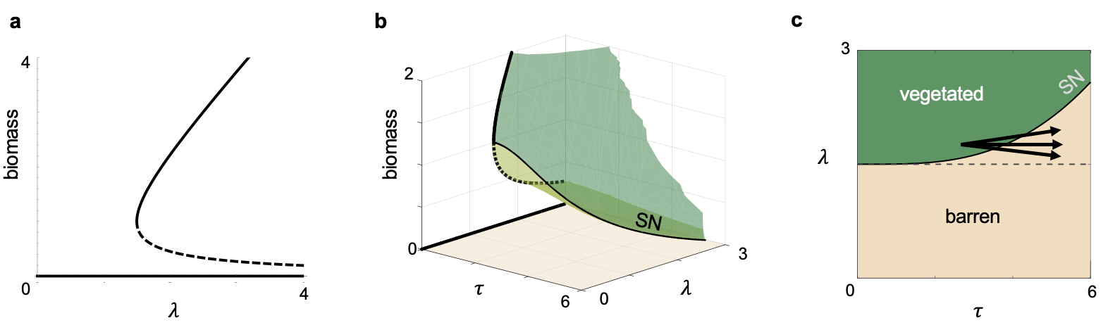
Figure 4: (a) Equilibrium biomass in the continuous nonspatial Klausmeier model (56) with $m=0.75$, which yields a saddle-node bifurcation at $\lambda=1.5$. Solid and dashed lines represent stable and unstable branches of equilibria, respectively. (b) Continuation of fixed points and saddle-node bifurcation from continuous rain model (56) (in $\tau=0$ plane) to discrete rain model (58) (with $\tau>0$ and $\lambda$ variable). Dark green and tan surfaces contain stable fixed points; light green contains unstable fixed points. (c) By projecting (b) down the biomass axis onto the $(\tau,\lambda)$ disturbance parameter space, we obtain a stability diagram.

In contrast, we consider a flow-kick model of precipitation with the flow generated by the rain-free ODE

$$x_{1}^{\prime} =x_{2}x_{1}^{2}-mx_{1}$$ (57)

$$x_{2}^{\prime} =-x_{2}x_{1}^{2}-x_{2}.$$

The flow-kick map is then

$$\Phi_{\tau}(x;\lambda)=\varphi_{\tau}(x)+\tau\begin{bmatrix}0\\ \lambda\end{bmatrix}$$ (58)

where $\varphi_{\tau}(x)$ solves (57).

By Theorem 1, hyperbolic equilibria of the continuous rainfall model (56) continue locally to fixed points of the discrete rainfall model (58). Figure 4b illustrates biomass equilibrium branches for (56) in the $\tau=0$ plane as well as numerical continuations of vegetated flow-kick fixed points for $\tau>0$. A vertical section of this curved surface with fixed $\lambda$ traces out branches of flow-kick fixed points that continue from the ODE equilibria, except at the bifurcation point $\lambda=1.5$. In addition, one can analytically confirm that each vegetation-free equilibrium for (56) at $(0,\lambda)$ continues for $\tau>0$ to vegetation-free flow-kick fixed points at $(0,\tau\lambda/(1-e^{-\tau}))$.

Although flow-kick fixed points do not continue from the nonhyperbolic vegetated equilibrium with $\lambda=1.5$ fixed, the saddle-node bifurcation that occurs here in the ODE system (56) continues numerically in $\tau$ with $\lambda$ variable to the curves labeled SN in Figure 4bc. The 2D setting of the Klausmeier model exceeds the scope of Theorem 2, but we conjecture that Theorem 2 will generalize from 1D to higher dimensional systems using center manifold theory.

It is also of note that the precipitation rate $\lambda$ at which the saddle-node bifurcation occurs grows larger as the period between precipitation events $\tau$ increases. In other words, higher precipitation averages are needed to maintain vegetation when rain arrives in more intense, less frequent bursts. The model thus predicts that increases in the duration of droughts—with or without changes to average precipitation rates—could tip a system over the bifurcation curve from a vegetated to barren regime, as illustrated by the black arrows in Figure 4c.

Of course, precipitation events could be treated more realistically in a stochastic framework—for example, as a Poisson point process with exponentially distributed depths [22]. Gandhi and colleagues [23] recently coupled this approach with a spatially explicit reaction-diffusion model of vegetation and water dynamics. They found that the choice of deterministic versus stochastic rainfall events altered qualitative outcomes in some parameter regimes of the model, including the appearance of vegetation bands and their direction of migration. On the other hand, some insights from their stochastic framework align with our deterministic predictions. In particular, in scenarios of identically low mean annual precipitation rates, vegetation collapsed more quickly on average as the mean storm depth increased and mean arrival rates of storms decreased. Thus despite its limitations, a deterministic and non-spatial model of rainfall that resolves rain events in time can reveal patterns consistent with more realistic models.

The spatial and stochastic aspects of disturbance modeling that we have ignored for much of this paper are interesting directions for future research. For example, is it possible to predict general effects of discretizing disturbances, starting from a partial differential equation or stochastic differential equation model?

5.2 Predator-Prey Model

We use a predator-prey model to illustrate additional future directions for this work, including the continuation of periodic orbits, Hopf bifurcations, and transcritical bifurcations in $n$ dimensions.

The following ODE system models undisturbed prey ($x$) and predator ($y$) populations [24, 25], with parameters chosen to yield a stable limit cycle in the first quadrant:

$$\frac{dx}{dt} =x(1-x/4)-0.5y(1-e^{-1.5x})$$ (59)

$$\frac{dy}{dt} =-0.5y+y(1-e^{-0.5x}).$$

Consider disturbance to (59) in the form of proportional harvesting of the predator ($y$). On the one hand, a continuous model of this disturbance is

$$\frac{dx}{dt} =x(1-x/4)-0.5y(1-e^{-1.5x})$$ (60)

$$\frac{dy}{dt} =-0.5y+y(1-e^{-0.5x})-\lambda y,$$

where $\lambda$ controls the harvesting rate. On the other hand, a discrete model of this disturbance is given by the flow-kick map

$$\Phi_{\tau}(x,y;\lambda)=\varphi_{\tau}(x,y)-\tau\begin{bmatrix}0\\ \lambda[\varphi_{\tau}(x,y)]_{2}\end{bmatrix}$$ (61)

where $\varphi_{\tau}(x,y)$ solves (59) and $[\ \cdot\ ]_{2}$ takes its second component.

We compare dynamics and bifurcations across the continuous and discrete disturbance models. Harvesting pressure drives three qualitative regimes in the continuous system (60). As illustrated in Figure 5a for $\lambda=1/15$, low values of the harvesting parameter preserve a stable limit cycle $\Gamma$ that encloses an unstable coexistence equilibrium $P$. As $\lambda$ increases, the limit cycle contracts and undergoes a supercritical Hopf bifurcation at $\lambda_{*}\approx 0.089$, yielding a stable coexistence equilibrium $R$ in the first quadrant (Figure 5b). As $\lambda$ increases further, this equilibrium moves towards the saddle at $Q=(4,0)$. The two equilibria collide in a transcritical bifurcation at $\lambda_{**}\approx 0.365$, and for larger harvesting rates the point $Q$ is stable (Figure 5c). Thus the continuous model predicts either cycles of predator and prey populations, steady coexistence, or crash of the predators, depending on harvesting rates.

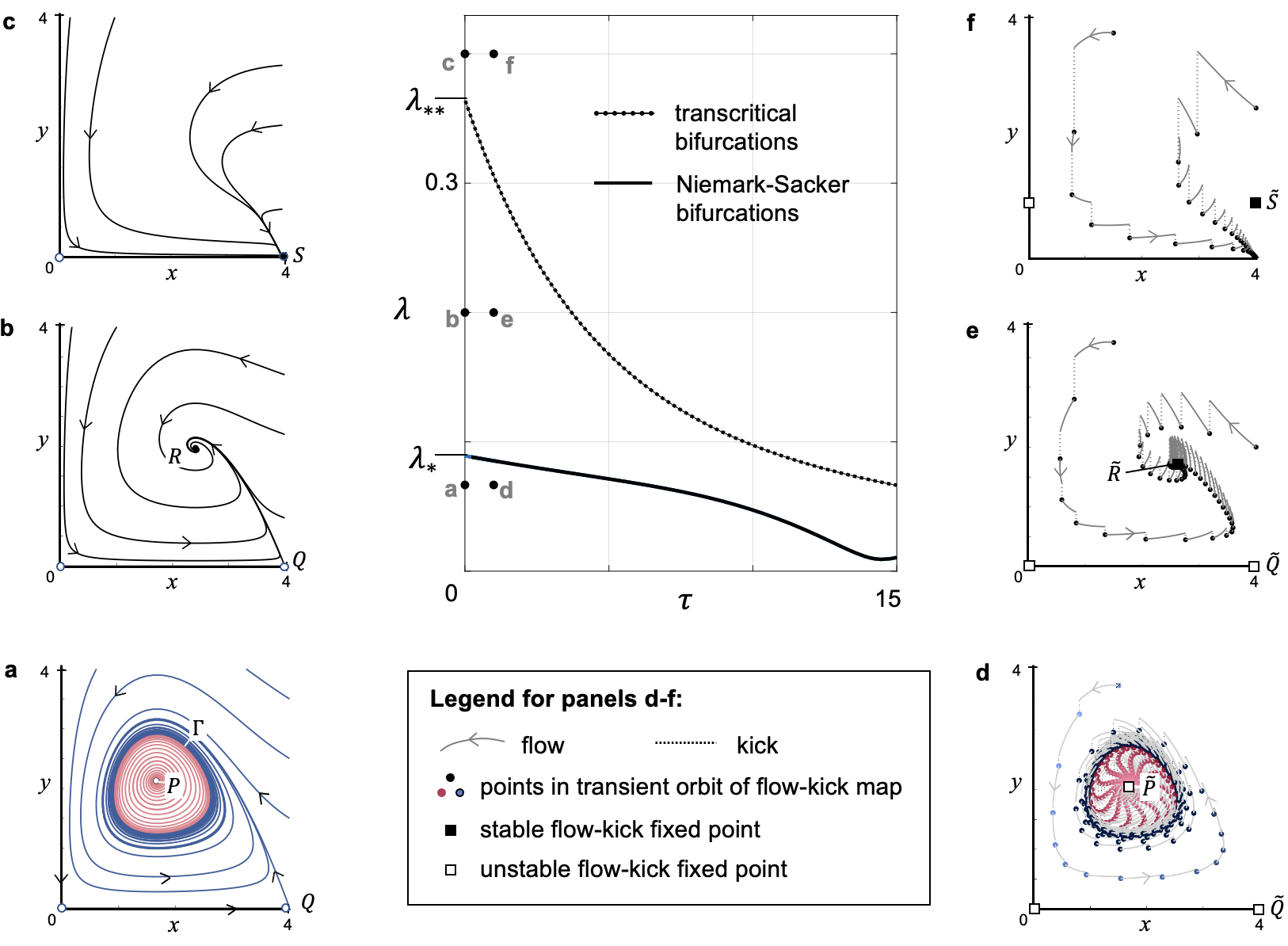
Figure 5: Predator prey dynamics under continuous and discrete disturbance harvests of predators. (a)-(c) Phase diagrams for the continuous model (visualized at $\tau=0$ in the central panel), showing three qualitative states of the system for disturbance rates $\lambda=1/15$ (panel a), $\lambda=1/5$ (panel b), and $\lambda=2/5$ (panel c). (d)-(f) Phase diagrams for flow-kick systems at disturbance rates matching (a)-(c), respectively, with $\tau=1$. Qualitative behaviors are similar between continuous and discrete disturbance models. Center panel: Continuation of transcritical and Hopf bifurcations in continuous disturbance model to transcritical and Niemark-Sacker bifurcations in the flow-kick disturbance model. Note that this diagram may be incomplete as a stability diagram, because the flow-kick system may have additional bifurcations that are disconnected from the $\tau=0$ axis.

The discrete disturbance model yields similar dynamics and predictions for small recovery times $\tau$. The rightmost panels d, e, and f in Figure 5 give flow-kick phase portraits for $\tau=1$ and values of $\lambda$ that match the continuous systems depicted in the leftmost panels a, b, and c, respectively. As Theorem 1 predicts, the hyperbolic equilibria at $P$, $Q$, $R$, and $O$ (the origin) in the continuous harvesting model continue to flow-kick fixed points with the same stabilities at $\tilde{P}$, $\tilde{Q}$, $\tilde{R}$, and $\tilde{O}$ in the discrete harvesting model. One subtle difference in dynamics is best understood by returning to an impulsive ODE framework: when we account for distinct flow and kick phases, a flow-kick fixed point does not necessarily represent unchanging populations. For example, the fixed point $\tilde{R}$ occurs where transient predator growth balances harvests, and both processes occur during one iteration of the flow-kick map. On the other hand, because the origin and $Q=\tilde{Q}=(4,0)$ are invariant under the flows generated by (59) and (60) as well as the kick to $y$, these points are both flow-kick fixed points and true equilibria of the impulsive DE across all values of $\tau$ and $\lambda$.

In addition to the similarities predicted by Theorem 1, the numerical simulations of predator-prey dynamics in Figure 5 display several patterns that warrant further study. First, the fixed points that continue retain not only their stabilities but also their type—for example, node, spiral, or saddle. We conjecture that equilibrium type continues in general from ODE to flow-kick systems when the type in the ODE system is not degenerate. Second, the stable limit cycle $\Gamma$ in Figure 5a has a striking counterpart in Figure 5d: flow-kick trajectories tend towards what appears to be an invariant closed curve near $\Gamma$. Our numerical simulation does not distinguish high-period periodic points from a dense orbit along an invariant curve, but in either case the cycling of predator and prey species in the flow-kick system closely mimics that of the continuous system. Continuation of periodic orbits from ODEs to analogous structures in flow-kick models represents another area for future study.

The predator-prey example also provides evidence for bifurcation continuation beyond the scope of rigorous results in this paper. The central panel in Figure 5 plots bifurcation curves for the flow-kick map in $(\tau,\lambda)$ parameter space. We used MatcontM to identify a curve of Niemark-Sacker bifurcations (solid black line), which connects to the continuous Hopf bifurcation at $(0,\lambda_{*})$. Given that Hopf bifurcations are generic, we conjecture that few additional conditions will be needed to guarantee that they continue from ODE systems to Niemark-Sacker bifurcations in flow-kick systems. Furthermore, although MatcontM does not continue transcritical bifurcations, we developed an ansatz condition

$$\lambda\tau=1-\text{exp}(\tau(1/2-e^{-2}))$$ (62)

necessary for a transcritical bifurcation to occur at $(x,y)=(4,0)$ (see Appendix C). The dashed curve represents this condition, which we confirmed numerically as a transcritical bifurcation at test points between $\tau=0$ and $\tau=15$. The curve connects to the ODE transcritical bifurcation at $(0,\lambda_{**})$. As with saddle-node bifurcations, we expect that central manifold theory will allow future rigorous results on continuation of transcritical bifurcations in $n$ dimensions.

Lastly, despite the continuation patterns that the predator prey system illustrates for small $\tau$, larger $\tau$ values can destroy qualitative similarities between ODE and flow-kick disturbance models. For example, even though $\lambda=0.2$ predicts stable coexistence between predators and prey when $\tau=1$, increasing the time between harvests to $\tau=4$ changes the prediction to predator crash (point $g$ in Figure 5, central panel).

6 Discussion

We have presented both rigorous arguments and numerical evidence that ODE and flow-kick disturbance models resemble one another when the kicks occur at high frequencies. On the one hand, flow-kick maps $\Phi_{\tau}$ with the same average disturbance rate generate a vector field with that disturbance rate in the limit as $\tau$—the period between kicks—decreases to zero (Proposition 1). On the other hand, we have seen multiple dynamic features of ODE disturbance models continue locally to flow-kick disturbance models. These include fixed points with their stabilities (Theorem 1), saddle node bifurcations in 1D systems (Theorem 2) and 2D systems (Figure 4), and transcritical bifurcations in 1D systems (Theorem 3) and 2D systems (Figure 5). Future work in this direction could (i) embed the saddle-node and transcritical continuation results in higher-dimensional systems and (ii) treat continuation of periodic orbits and Hopf bifurcations in ODE disturbance models to analogous structures in flow-kick systems, as observed in Figure 5. These proven and conjectured patterns point towards a consistent take-away: if true disturbances are discrete and high-frequency, but we choose to model them with an ODE instead, then dynamic structures in the ODE model approximate similar structures in the kicked system.

However, this story changes as disturbance frequency decreases. Although saddle-node and transcritical bifurcations do persist from 1D continuous to flow-kick systems, they can occur at different disturbance rates. This phenomenon was previously observed for additively harvested populations with logistic growth [5] and with an Allee effect [4]. It also appears in the Klausmeier model of vegetation and precipitation (section 5.1) and the harvested predator-prey system (section 5.2). In the Klausmeier model, an increase in the bifurcation value of the rainfall parameter $\lambda$ as return time $\tau$ increases means that that higher average precipitation rates are needed to maintain a stable vegetated equilibrium as the time between precipitation events becomes longer. In the predator-prey model, sustainable harvesting of the predator population requires lower harvesting rates when harvests are discretized, more spread out (and more intense) because the transcritical bifurcation that represents predator collapse occurs at a lower value of the harvesting parameter $\lambda$ as the recovery period $\tau$ increases. As noted by [4] and [5], these patterns have real implications for a system’s resilience to disturbance. First, we may underestimate a system’s vulnerability to regime changes if we smooth out the discrete quality of disturbances in our models. Second, changes to the timing of real-world disturbances—while maintaining the same average disturbance rate—can drive tipping.

In addition to changing bifurcation thresholds, increasing the flow times between kicks can introduce entirely new dynamics not observed in the continuous system. In a discrete model of fire disturbances to a tree-grass savannah, Hoyer-Leitzel and Iams found curves of bifurcations in disturbance space that are isolated away from the origin—bifurcations that occur in the flow-kick systems but not in their continuous analog [6]. It should be noted that the kick structure in [6] differs from Definition 5, with the disturbance rate dependent on $\tau$ as well as $x$. Nonetheless, this example alerts us that accounting for the discrete nature of disturbance could reveal bifurcation structures absent from an averaged ODE model. We suspect this is true for the predator-prey model in particular, since Neimark-Sacker bifurcations can undergo resonance bifurcations, leading to regions of period doubling or chaos. In this way, studying what dynamics flow-kick models not only maintain but also gain relative to their ODE counterparts represents a rich area for future study.

Appendix A

Deriving Integral Forms of Remainder

Claim 1: If $f$ is of class $C^{k+1}$ on an open interval $I\subset\mathbb{R}$ with a base point $a\in I$ and the variable $t\in I$, then

$$f(t)=\sum_{j=0}^{k}\frac{f^{(j)}(a)}{j!}(t-a)^{j}+R_{k,a}(t)$$

where $\displaystyle R_{k,a}(t)=\frac{1}{k!}\int_{a}^{t}(t-u)^{k}f^{(k+1)}(u)du$.

Proof: We proceed by induction on $k$.
Base case ($k=0$): The claim reduces to $\displaystyle f(t)=f(a)+\int_{a}^{t}f^{\prime}(u)du$. This is the Fundamental Theorem of Calculus.

Intuition building ($k=1$): We have $\displaystyle f(t)=f(a)+\int_{a}^{t}f^{\prime}(u)du$. Integrate $\displaystyle\int_{a}^{t}f^{\prime}(u)du$ by parts:

$$\begin{array}[]{cccc}\text{let }&g=f^{\prime}(u)&\text{and}&dh=du\\ \text{so }&dg=f^{(2)}(u)du&\text{and }&h=u-t.\end{array}$$

(Note the strategic choice of $u-t$ rather than simply $u$ for the antiderivative $h$.) To integrate by parts, we write

$$\int_{a}^{t}g\ dh =gh\Big{|}_{a}^{t}-\int_{a}^{t}h\ dg$$

$$\text{so }\hskip 28.45274pt\int_{a}^{t}f^{\prime}(u)\ du =f^{\prime}(u)(u-t)\Big{|}_{a}^{t}-\int_{a}^{t}(u-t)f^{(2)}(u)du$$

$$=f^{\prime}(t)(t-t)-f^{\prime}(a)(a-t)-\int_{a}^{t}(u-t)f^{(2)}(u)du$$

$$=f^{\prime}(a)(t-a)+\int_{a}^{t}(t-u)f^{(2)}(u)du$$

Thus we have

$$f(t)=f(a)+f^{\prime}(a)(t-a)+\frac{1}{1!}\int_{a}^{t}(t-u)f^{(2)}(u)du.$$

In this way, we see the Taylor series is falling out of the Fundamental Theorem of Calculus plus integration by parts.

Inductive hypothesis: Assume

$$f(t) =\sum_{j=0}^{k-1}\frac{f^{(j)}(a)}{j!}(t-a)^{j}+R_{k-1,a}(t)$$ (63)

$$\text{where }\hskip 14.22636ptR_{k-1,a}(t) =\frac{1}{(k-1)!}\int_{a}^{t}(t-u)^{k-1}f^{(k)}(u)du.$$

Inductive step: Integrate the remainder $R_{k-1,a}(t)$ by parts!

$$\begin{array}[]{cccc}\text{Let }&g=f^{(k)}(u)&\text{and}&dh=(t-u)^{k-1}du\\ \text{so }&dg=f^{(k+1)}(u)du&\text{and }&h=-\frac{1}{k}(t-u)^{k}.\end{array}$$

Then

$$\frac{1}{(k-1)!}\int_{a}^{t}\underbrace{f^{(k)}(u)}_{g}\underbrace{(t-u)^{k-1}du}_{dh} =\frac{1}{(k-1)!}\left[-\frac{1}{k}(t-u)^{k}f^{(k)}(u)\Big{|}_{a}^{t}+\frac{1}{k}\int_{a}^{t}(t-u)^{k}f^{(k+1)}(u)du\right]$$

$$=\frac{1}{(k-1)!}\left[\frac{1}{k}(t-a)^{k}f^{(k)}(a)+\frac{1}{k}\int_{a}^{t}(t-u)^{k}f^{(k+1)}(u)du\right]$$

$$=\frac{f^{(k)}(a)}{k!}(t-a)^{k}+\frac{1}{k!}\int_{a}^{t}(t-u)^{k}f^{(k+1)}(u)du.$$

Substituting this new form of the remainder into our expression (63) for $f(t)$, we get

$$f(t) =\underbrace{\sum_{j=0}^{k-1}\frac{f^{(j)}(a)}{j!}(t-a)^{j}+\frac{f^{(k)}(a)}{k!}(t-a)^{k}}_{\sum_{j=0}^{k}\frac{f^{(j)}(a)}{j!}(t-a)^{j}}+\underbrace{\frac{1}{k!}\int_{a}^{t}(t-u)^{k}f^{(k+1)}(u)du}_{R_{k,a}(t)}$$

as desired. ∎

The integral form of the remainder in Claim 1 is standard, but the desired factors of $t$ are hidden in the domain of integration. We make them explicit in Claim 2, which follows from a linear change of variables on the variable of integration.

Claim 2: If $f$ is of class $C^{k+1}$ on an open interval $I\subset\mathbb{R}$ with a base point $a\in I$ and the variable $t\in I$, then

$$f(t)=\sum_{j=0}^{k}\frac{f^{(j)}(a)}{j!}(t-a)^{j}+R_{k,a}(t)\$$

where $\displaystyle R_{k,a}(t)=\frac{(t-a)^{k+1}}{k!}\int_{0}^{1}(1-v)^{k}f^{(k+1)}(a+v(t-a))dv$.

Proof: The only difference between Claim 1 and Claim 2 is the form of the remainder, so it suffices to prove that the two integrals

$$\frac{1}{k!}\int_{a}^{t}(t-u)^{k}f^{(k+1)}(u)du\hskip 14.22636pt\text{and}\hskip 14.22636pt\frac{(t-a)^{k+1}}{k!}\int_{0}^{1}(1-v)^{k}f^{(k+1)}(a+v(t-a))dv$$

are equal. We accomplish this by the change of variables $u=a+v(t-a)$, which transforms…

the bound $u=a$	to	$v=0$
the bound $u=t$	to	$v=1$
the factor $(t-u)^{k}$	to	$(t-(a+v(t-a)))^{k}=((1-v)(t-a))^{k}$
the factor $f^{(k+1)}(u)$	to	$f^{(k+1)}(a+v(t-a))$
the differential $du$	to	$(t-a)dv$

and equality of the two integrals follows. ∎

When we expand $\varphi(\tau,x)$ in $\tau$ in Proposition 2 and thereafter, we use Claim 2 with $k=1$, $a=0$, $t=\tau$, and $f(\cdot)=\varphi(\cdot,x)$.

Appendix B

Further details on the proof of Theorem 3

(iv) Mixed partials: First we compute derivatives to see that

$$\frac{\partial^{2}\Phi_{\tau}}{\partial x\partial\lambda}(0,\lambda_{\tau}) =\frac{\partial}{\partial x}\Big{[}\frac{\partial}{\partial\lambda}\Big{[}\varphi_{\tau}(x)+\tau\varphi_{\tau}(x)\,s(\varphi_{\tau}(x);\lambda)\Big{]}\Big{]}\Big{|}_{\tiny\begin{array}[]{l}x=0\\ \lambda=\lambda_{\tau}\end{array}}$$ (66)

$$=\frac{\partial}{\partial x}\Big{[}\tau\varphi_{\tau}(x)\,\frac{\partial s}{\partial\lambda}(\varphi_{\tau}(x);\lambda)\Big{]}\Big{|}_{\tiny\begin{array}[]{l}x=0\\ \lambda=\lambda_{\tau}\end{array}}$$ (69)

$$=\tau\Big{(}\frac{\partial\varphi_{\tau}}{\partial x}\frac{\partial s}{\partial\lambda}(x;\lambda)+\varphi_{\tau}(x)\frac{\partial^{2}s}{\partial x\partial\lambda}(\varphi_{\tau}(x);\lambda)\Big{)}\Big{|}_{\tiny\begin{array}[]{l}x=0\\ \lambda=\lambda_{\tau}\end{array}}$$ (72)

$$=\tau\frac{\partial\varphi_{\tau}}{\partial x}(0)\frac{\partial s}{\partial\lambda}(0;\lambda_{\tau}).$$ (73)

The factor of $\tau$ in (73) is greater than zero for flow-kick maps. The factor $\frac{\partial\varphi_{\tau}}{\partial x}(0)$ evaluates to $1$ at $\tau=0$ (as $\varphi_{0}$ is the identity map), so $\frac{\partial\varphi_{\tau}}{\partial x}(0)$ remains nonzero locally for $\tau>0$. Lastly, from the mixed partials condition (iv) in the continuous system and equations (50), we know that $\frac{\partial s}{\partial\lambda}(0;\lambda_{*})\not=0$. And because $\lambda_{\tau}$ varies continuously from $\lambda_{0}=\lambda_{*}$ and $s$ is $C^{1}$, the derivative $\frac{\partial s}{\partial\lambda}(0,\lambda_{\tau})$ remains nonzero for sufficiently small $\tau$. It follows that $\frac{\partial^{2}\Phi_{\tau}}{\partial x\partial\lambda}(0,\lambda_{\tau})\not=0$ locally.

(v) Quadratic dominance: The first derivative of the flow-kick map

$$\Phi_{\tau}(x,\lambda)=\varphi_{\tau}(x)+\tau\varphi_{\tau}(x)s(\varphi_{\tau}(x),\lambda)$$

with respect to $x$ is

$$\frac{\partial\Phi_{\tau}}{\partial x} =\frac{\partial\varphi_{\tau}}{\partial x}+\tau\frac{\partial\varphi_{\tau}}{\partial x}s(\varphi_{\tau}(x),\lambda)+\tau\varphi_{\tau}(x)\frac{\partial s}{\partial u}\frac{\partial\varphi_{\tau}}{\partial x}.$$ (74)

The second derivative with respect to $x$ is

$$\begin{split}\frac{\partial^{2}\Phi_{\tau}}{\partial x^{2}}&=\frac{\partial^{2}\varphi_{\tau}}{\partial x^{2}}+\tau\frac{\partial^{2}\varphi_{\tau}}{\partial x^{2}}s(\varphi_{\tau}(x),\lambda)+2\tau\left(\frac{\partial\varphi_{\tau}}{\partial x}\right)^{2}\frac{\partial s}{\partial u}\\ &\hskip 128.0374pt+\tau\varphi_{\tau}(x)\frac{\partial^{2}s}{\partial u^{2}}\left(\frac{\partial\varphi_{\tau}}{\partial x}\right)^{2}+\tau\varphi_{\tau}(x)\frac{\partial s}{\partial u}\frac{\partial^{2}\varphi_{\tau}}{\partial x^{2}}.\end{split}$$ (75)

When we evaluate at a point $(x_{\tau},\lambda_{\tau})=(0,\lambda_{\tau})$ along the curve of nonhyperbolic fixed points, (75) simplifies to

$$\frac{\partial^{2}\Phi_{\tau}}{\partial x^{2}}(0,\lambda_{\tau})=\frac{\partial^{2}\varphi_{\tau}}{\partial x^{2}}(0)+\tau\frac{\partial^{2}\varphi_{\tau}}{\partial x^{2}}(0)s(0,\lambda_{\tau})+2\tau\left(\frac{\partial\varphi_{\tau}}{\partial x}(0)\right)^{2}\frac{\partial s}{\partial x}(0,\lambda_{\tau})$$ (76)

because $\varphi_{\tau}(0)=0$. We replace the first occurrence of $\frac{\partial^{2}\varphi_{\tau}}{\partial x^{2}}(0)$ in (76) with

$$\frac{\partial^{2}\varphi_{\tau}}{\partial x^{2}}(0) =\frac{\partial^{2}}{\partial x^{2}}\left.\left[x+\tau(xg(x))+\tau^{2}\int_{0}^{1}(1-v)\frac{\partial^{2}\varphi}{\partial t^{2}}(v\tau,x)dv\right]\right|_{x=0}$$ (77)

$$=2\tau\frac{dg}{dx}(0)+\tau^{2}\int_{0}^{1}(1-v)\frac{\partial^{4}\varphi}{\partial x^{2}\partial t^{2}}(v\tau,0)dv$$ (78)

and factor, yielding

$$\begin{split}\frac{\partial^{2}\Phi_{\tau}}{\partial x^{2}}(0,\lambda_{\tau})&=\tau\Bigg{(}2\frac{dg}{dx}(0)+\left(\frac{\partial\varphi_{\tau}}{\partial x}(0)\right)^{2}\frac{\partial s}{\partial x}(0,\lambda_{\tau})\\ &\hskip 113.81102pt+\frac{\partial^{2}\varphi_{\tau}}{\partial x^{2}}(0)s(0,\lambda_{\tau})+\tau\int_{0}^{1}(1-v)\frac{\partial^{4}\varphi}{\partial x^{2}\partial t^{2}}(v\tau,0)dv\Bigg{)}\end{split}$$ (79)

The first factor of $\tau$ in (79) is nonzero for flow-kick maps. The second factor is a continuous function of $\tau$ that at $\tau=0$ takes the value

$$2\Big{(}\frac{dg}{dx}(0)+\frac{\partial s}{\partial x}(0;\lambda_{*})\Big{)}.$$ (80)

(Note that the identity map $\varphi_{0}$ has first spatial derivative $1$ and second spatial derivative $0$.)

The quadratic dominance property in the ODE system gives

$$0 \not=\frac{\partial^{2}}{\partial x^{2}}\Big{[}x\,g(x)+x\,s(x;\lambda)\Big{]}\Big{|}_{\tiny\begin{array}[]{l}x=0\\ \lambda=\lambda_{*}\end{array}}$$ (83)

$$=\frac{\partial}{\partial x}\Big{[}g(x)+s(x;\lambda)+x\big{(}\frac{dg}{dx}+\frac{\partial s}{\partial x}\big{)}\Big{]}\Big{|}_{\tiny\begin{array}[]{l}x=0\\ \lambda=\lambda_{*}\end{array}}$$ (86)

$$=\Big{(}2\big{(}\frac{dg}{dx}+\frac{\partial s}{\partial x}\big{)}+x\big{(}\frac{d^{2}g}{dx^{2}}+\frac{\partial^{2}s}{\partial x^{2}}\big{)}\Big{)}\Big{|}_{\tiny\begin{array}[]{l}x=0\\ \lambda=\lambda_{*}\end{array}}$$ (89)

$$=2\Big{(}\frac{dg}{dx}(0)+\frac{\partial s}{\partial x}(0;\lambda_{*})\Big{)}$$ (90)

Hence (80) is nonzero, and since the second factor in (79) is continuous in $\tau$ it remains nonzero close to $\tau=0$. It follows that $\frac{\partial^{2}\Phi_{\tau}}{\partial x^{2}}(0,\lambda_{\tau})$ is nonzero for $\tau$ sufficiently small, so quadratic dominance holds locally for the flow-kick maps.

Appendix C

Conjecture: For the predator-prey flow-kick map given by equation (61), a necessary condition for a transcritical bifurcation at the point (4,0) is $\lambda\tau=1-e^{-a\tau}$ where $a=1/2-e^{-2}$.

Derivation: Let $\Phi_{\tau}(x,y)=\begin{bmatrix}[\varphi_{\tau}(x,y)]_{1}\\ [\varphi_{\tau}(x,y)]_{2}-\tau\lambda[\varphi_{\tau}(x,y)]_{2}\end{bmatrix}\equiv\begin{bmatrix}U(x,y)\\ V(x,y)\end{bmatrix}$. We have used subscripts of $1$ and $2$ on the flow function $\varphi$ to denote its $x$ and $y$ components, respectively. For all values of the disturbance parameters $\tau$ and $\lambda$, (4,0) is a fixed point for the map; that is,

$$\left\{\begin{array}[]{ll}4&=U(4,0)\\ 0&=V(4,0).\end{array}\right.$$ (91)

A transcritical bifurcation occurs at (4,0) when the branch of fixed points at (4,0) crosses a distinct branch of fixed points $(\hat{x},\hat{y})$. This branch of fixed points also satisfies $V(\hat{x},\hat{y})=\hat{y}$, or equivalently $\hat{y}-V(\hat{x},\hat{y})=0$. Thus the transcritical bifurcation occurs when $y-V(4,y)=0$ has $y=0$ as a double root.

To approximate $V(4,y)$, we fix the value of $x$ at $4$ in the second equation of (59), giving

$$\frac{dy}{dt} =-0.5y+y(1-e^{-2})$$ (92)

$$=(1/2-e^{-2})y.$$

Integrating (92) yields $y(t)=y_{0}e^{a\tau}$ where $a=(1/2-e^{-2})$. We use $ye^{a\tau}$ to approximate $[\varphi_{\tau}(4,y)]_{2}$, noting that the approximation is exact at $y=0$. Then

$$V(4,y)\approx ye^{a\tau}-\tau\lambda ye^{a\tau}=(1-\tau\lambda)ye^{a\tau}.$$ (93)

With the approximation (93) for $V(4,y)$, we rewrite $y-V(4,y)=0$ as

$$y-(1-\tau\lambda)ye^{a\tau} =0$$ (94)

$$\iff y(1-(1-\tau\lambda)e^{a\tau}) =0.$$ (95)

Now at $y=0$ equation (95) is equivalent to the fixed point condition $y-V(4,y)=0$. Requiring that this equation has a double root at $y=0$ amounts to requiring

$$1-(1-\tau\lambda)e^{a\tau} =0$$ (96)

$$\iff\tau\lambda=1-e^{-a\tau}.$$ (97)

∎

References

• [1] Francesco Accatino, Carlo De Michele, Renata Vezzoli, Davide Donzelli, and Robert J Scholes. Tree–grass co-existence in savanna: Interactions of rain and fire. Journal of Theoretical Biology, 267(2):235–242, 2010.
• [2] Christopher A Klausmeier. Regular and irregular patterns in semiarid vegetation. Science, 284(5421):1826–1828, 1999.
• [3] Vangipuram Lakshmikantham, Pavel S Simeonov, et al. Theory of Impulsive Differential Equations, volume 6. World Scientific, 1989.
• [4] Katherine Meyer, Alanna Hoyer-Leitzel, Sarah Iams, Ian Klasky, Victoria Lee, Stephen Ligtenberg, Erika Bussmann, and Mary Lou Zeeman. Quantifying resilience to recurrent ecosystem disturbances using flow–kick dynamics. Nature Sustainability, 1(11):671–678, 2018.
• [5] Mary Lou Zeeman, Katherine Meyer, Erika Bussmann, Alanna Hoyer-Leitzel, Sarah Iams, Ian J Klasky, Victoria Lee, and Stephen Ligtenberg. Resilience of socially valued properties of natural systems to repeated disturbance: A framework to support value-laden management decisions. Natural Resource Modeling, 31(3):e12170, 2018.
• [6] Alanna Hoyer-Leitzel and Sarah Iams. Impulsive fire disturbance in a savanna model: Tree–grass coexistence states, multiple stable system states, and resilience. Bulletin of Mathematical Biology, 83(11):1–25, 2021.
• [7] Stephen Ippolito, Vincent Naudot, and Erik G Noonburg. Alternative stable states, coral reefs, and smooth dynamics with a kick. Bulletin of Mathematical Biology, 78(3):413–435, 2016.
• [8] Tom Chou and Maria R D’Orsogna. A mathematical model of reward-mediated learning in drug addiction. Chaos: An Interdisciplinary Journal of Nonlinear Science, 32(2), 2022.
• [9] A Tchuinté Tamen, Yves Dumont, Jean Jules Tewa, Samuel Bowong, and Pierre Couteron. Tree–grass interaction dynamics and pulsed fires: Mathematical and numerical studies. Applied Mathematical Modelling, 40(11-12):6165–6197, 2016.
• [10] A Tchuinté Tamen, Yves Dumont, Jean-Jules Tewa, Samuel Bowong, and Pierre Couteron. A minimalistic model of tree–grass interactions using impulsive differential equations and non-linear feedback functions of grass biomass onto fire-induced tree mortality. Mathematics and Computers in Simulation, 133:265–297, 2017.
• [11] Mark E Ritchie and Jacob F Penner. Episodic herbivory, plant density dependence, and stimulation of aboveground plant production. Ecology and Evolution, 10(12):5302–5314, 2020.
• [12] Alexander Fulk, Weizhang Huang, Folashade Agusto, et al. Exploring the effects of prescribed fire on tick spread and propagation in a spatial setting. Computational and Mathematical Methods in Medicine, 2022, 2022.
• [13] Alanna Hoyer-Leitzel, Sarah Iams, Alanna Haslam-Hyde, Mary Lou Zeeman, and Nina Fefferman. An immuno-epidemiological model for transient immune protection: A case study for viral respiratory infections. Infectious Disease Modelling, 8(3):855–864, 2023.
• [14] Qiudong Wang and Lai-Sang Young. Strange attractors in periodically-kicked limit cycles and hopf bifurcations. Communications in Mathematical Physics, 240:509–529, 2003.
• [15] Kevin K. Lin and Lai-Sang Young. Dynamics of periodically kicked oscillators. Journal of Fixed Point Theory and Applications, 7:291–312, 2010.
• [16] Vincent Naudot, Shane Kepley, and William D Kalies. Complexity in a hybrid van der Pol system. International Journal of Bifurcation and Chaos, 31(13):2150194, 2021.
• [17] Gerald Folland. Remainder estimates in Taylor’s theorem. The American Mathematical Monthly, 97(3):233–235, 1990.
• [18] G.W. Stewart and Ji-guang Sun. Matrix Perturbation Theory. Academic Press, 1990.
• [19] Stephen Wiggins. Introduction to Applied Nonlinear Dynamical Systems and Chaos, volume 2. Springer, 1990.
• [20] Annick Dhooge, Willy Govaerts, Yu A Kuznetsov, Hil Gaétan Ellart Meijer, and Bart Sautois. New features of the software MatCont for bifurcation analysis of dynamical systems. Mathematical and Computer Modelling of Dynamical Systems, 14(2):147–175, 2008.
• [21] Hil Meijer, Willy Govaerts, Yuri A Kuznetsov, R Khoshsiar Ghaziani, and Niels Neirynck. MatContM, a toolbox for continuation and bifurcation of cycles of maps: Command line use. Department of Mathematics, Utrecht University, 2017.
• [22] Ignacio Rodriguez-Iturbe, Amilcare Porporato, Luca Ridolfi, V Isham, and DR Coxi. Probabilistic modelling of water balance at a point: The role of climate, soil and vegetation. Proceedings of the Royal Society of London. Series A: Mathematical, Physical and Engineering Sciences, 455(1990):3789–3805, 1999.
• [23] Punit Gandhi, Lily Liu, and Mary Silber. A pulsed-precipitation model of dryland vegetation pattern formation. SIAM Journal on Applied Dynamical Systems, 22(2):657–693, 2023.
• [24] Michael L Rosenzweig. Paradox of enrichment: Destabilization of exploitation ecosystems in ecological time. Science, 171(3969):385–387, 1971.
• [25] Robert M May. Limit cycles in predator-prey communities. Science, 177(4052):900–902, 1972.