Rigidity of flat holonomies

Abstract.

We prove that the existence of one horosphere in the universal cover of a closed, strictly quarter pinched, negatively curved Riemannian manifold of dimension $n\geq 3$ on which the stable holonomy along minimizing geodesics coincide with the Riemannian parallel transport, implies that the manifold is homothetic to a real hyperbolic manifold.

0. Introduction

Mostow’s seminal rigidity theorem [15] asserts that the geometry of a closed hyperbolic manifold of dimension greater than two is determined by its fundamental group. Inspired by Mostow’s theorem, we undertake a study of related, yet, more general themes. In this paper, we look at natural geometric submanifolds, the horospheres, and ask to what extent do these determine the geometry of the whole manifold. Precisely, we are concerned with the following general question:

Question 0.1.

Does the geometry of the horospheres of a closed, negatively curved manifold of dimension greater than two, determine the geometry of the whole manifold?

In general, there are very few answers to Question 0.1, and all of these relate the extrinsic geometry of the horospheres to the geometry of $M$. For instance, by combining [4] and [5] (see [5], Corollary 9.18) one shows that if all the horospheres have constant mean curvature, then the underlying manifold is locally symmetric (of negative curvature). Let us recall that the mean curvature of a hypersurface is related to the derivative of its volume element in the normal direction to the hypersurface, and hence the mean curvature is an extrinsic quantity. In this paper, our main hypothesis is to relax the assumption on the sectional curvature in Mostow’s theorem and allow it to be strictly quarter negatively curved pinched. In this case constant mean curvature of the horospheres only occur for real hyperbolic manifolds (up to homothety). In contrast, we would like to emphasize that we only consider the intrinsic properties of the induced metric on the horospheres.

Before stating our main theorem, let us recall a few important features of the manifolds under consideration and results that are related to our work in this paper. Let $M$ denote an $(n+1)$-dimensional, closed, Riemannian manifold endowed with a metric of negative sectional curvature, $n\geq 2$. It follows from the Cartan-Hadamard theorem that $\tilde{M}$, the universal cover of $M$, is diffeomorphic to $\mathbb{R}^{n+1}$. Once endowed with the pull-back Riemannian metric from $M$, the geometric boundary $\partial\tilde{M}$ of $\tilde{M}$, is by definition the set of equivalence classes of geodesic rays in $\tilde{M}$, where two geodesic rays are equivalent if they remain at a bounded Hausdorff distance. We recall that, in our context, it is homeomorphic to $\mathbb{S}^{n}$.

Given a point, $x_{0}\in\tilde{M}$, and a unit tangent vector, $\tilde{v}\in T_{x_{0}}\tilde{M}$, we let $c_{\tilde{v}}$ denote the unique geodesic ray determined by $c_{\tilde{v}}(0)=x_{0}$ and $\dot{c}_{\tilde{v}}(0)=\tilde{v}$. It is well known that the map, $\tilde{v}\in T_{x_{0}}\tilde{M}\mapsto[c_{\tilde{v}}]\in\partial\tilde{M}$, defines a homeomorphism between the unit sphere in $T_{x_{0}}\tilde{M}$ and $\partial\tilde{M}$. Given a point $\xi=[c_{\tilde{v}}]\in\partial\tilde{M}$, the Busemann function $B_{\xi}(\cdot)$ is then defined for all $\xi\in\partial\tilde{M}$ and for all $x\in\tilde{M}$, by $B_{\xi}(x)=\lim_{t\to\infty}(d(x,c_{\tilde{v}}(t))-d(x_{0},c_{\tilde{v}}(t)))$.

Since $M$ is a closed negatively curved manifold, for each $\xi\in\partial\tilde{M}$ it is known that the Busemann function $B_{\xi}(\cdot)$ is $C^{\infty}$-smooth. Furthermore, for any $t\in\mathbb{R}$, the level set

$$H_{\xi}(t)=\left\{x\in{\tilde{M}};\,B_{\xi}(x)=t\right\}$$

is a smooth submanifold of $\tilde{M}$ which is diffeomorphic to $\mathbb{R}^{n}$ and which is called a horosphere centred at $\xi$. The sublevel set

$$HB_{\xi}(t)=\left\{x\in{\tilde{M}};\,B_{\xi}(x)\leq t\right\}$$

is called a horoball. It follows that horospheres inherit a complete Riemannian metric induced by the restriction of the metric of $\tilde{M}$. For instance, if $(M,g)$ is a real hyperbolic manifold, every horosphere of $\tilde{M}$ is flat and therefore isometric to the Euclidean space $\mathbb{R}^{n}$.

So far we defined horospheres as special submanifolds in $\tilde{M}$. However, a dynamical perspective turns out to be important in the proof of the main theorem. Let $\tilde{p}:T^{1}\tilde{M}\rightarrow\tilde{M}$ and $p:T^{1}M\rightarrow M$ denote the natural projections. The geodesic flow $\tilde{g}_{t}$ on $T^{1}\tilde{M}$ is known to be an Anosov flow, that is, the tangent bundle $TT^{1}\tilde{M}$ admits a decomposition as $TT^{1}\tilde{M}=\mathbb{R}X\oplus\tilde{E}^{ss}\oplus\tilde{E}^{su}$, where $X$ is the vector field generating the geodesic flow and $\tilde{E}^{ss}$, $\tilde{E}^{su}$ are the strong stable and strong unstable distributions, respectively. These distributions are known to be integrable, invariant under the differential $d\tilde{g}_{t}$ of the geodesic flow, and to give rise to two transverse foliations of $T^{1}\tilde{M}$, $\tilde{W}^{ss}$ and $\tilde{W}^{su}$, the strong stable and strong unstable foliations, respectively, whose leaves are smooth submanifolds. A classical property of these foliations is that in general they are transversally Hölder with exponent less than one, and when the sectional curvature, denoted by K is strictly $1/4$-pinched (i.e., $-4<K\leq-1$), they are transversally $C^{1}$ (see [11, page 226]), but we do not use such a regularity.

A link between the two point of views on horospheres is the following. For $\tilde{v}\in T^{1}\tilde{M}$, the strong stable leaf $\tilde{W}^{ss}(\tilde{v})$ through $\tilde{v}$ is defined to be the set of unit vectors $\tilde{w}\in T^{1}\tilde{M}$ which are normal to the horosphere $H_{\xi}(t)$ and pointing inward the horoball $HB_{\xi}(t)$ in the direction of $\xi=c_{\tilde{v}}(+\infty)$, with $t=B_{\xi}(\tilde{p}({\tilde{v}}))$ so that $H_{\xi}(t)=\tilde{p}(W^{ss}({\tilde{v}}))$.

With this notation in place, let us now describe our main theorem and the foundational work we build upon. In Section 2, we will recall the construction of the stable holonomy, introduced by Kalinin-Sadovskaya, [12] and Avila-Santamaria-Viana, [3]. It is a geodesic flow invariant family of isomorphisms $\Pi^{\xi}_{s}(x,y)$ between the tangent spaces to $H_{\xi}(s)$ at any two points $x$ and $y$. This construction requires the sectional curvature of $M$ to be strictly $1/4$-pinched. To the best of our knowledge, a stable holonomy cannot be defined without the pinching condition. On the other hand, every horosphere $H_{\xi}(s)$ carries the Riemannian metric induced by the one of $\tilde{M}$. In particular for every pair of sufficiently close points $x,y\in H_{\xi}(s)$, there a unique minimizing geodesic of $H_{\xi}(s)$ joining them. We thus may consider the parallel transport associated to the Levi-Civita connecion of the induced metric on $H_{\xi}(s)$, denoted by $P^{\xi}_{s}(x,y)$, between the tangent spaces to $H_{\xi}(s)$ at these points $x$ and $y$. As mentioned before, in the case of $K\equiv-1$, the induced Riemannian metric on horospheres is flat and the stable holonomy $\Pi^{\xi}_{s}(x,y)$ and the parallel transport $P^{\xi}_{s}(x,y)$ coincide for every pairs of points $x$ and $y$ on $H_{\xi}(s)$. Our main result is that the converse is true among $1/4$ -pinched negatively curved manifolds.

Theorem 0.2 (Main Theorem).

Let $M$ be a closed, Riemannian manifold of dimension $n\geq 3$, endowed with a strictly $1/4$-pinched negatively curved sectional curvature. Assume that there exists $\xi\in\partial\tilde{M}$ and $s\in\mathbb{R}$ such that for every pair of points $x,y\in H_{\xi}(s)$ joined by a unique minimizing geodesic, the stable holonomy $\Pi^{\xi}_{s}(x,y)$ is identical to the parallel transport $P_{s}^{\xi}(x,y)$. Then $(M,g)$ is homothetic to a real hyperbolic manifold.

As mentioned before, the restriction on the sectional curvature ensures the existence of the stable holonomy. For Theorem 0.2 to hold, it is indeed sufficient to make the assumption for a single horosphere in $\tilde{M}$ since in Proposition 1.1 we show that it implies that all horospheres satisfy it.

In the case that $\dim M=2$, Theorem 0.2, may still be true. However, our proof in the case $\dim M\geq 3$ does not apply since it relies on Theorems 0.3 and 0.5 which both require our assumption on the dimension, see more details below.

Essential to the proof of our main theorem is the following deep characterization of closed, real hyperbolic manifolds stated by Butler [6]. This result is related to the way the geometry of horospheres evolves under the action of the geodesic flow. Butler showed, in what might be called now as Lyapunov rigidity, that the equality of the modulus of the eigenvalues of $dg_{t}|E^{ss}(v)$ along every periodic geodesic has an important geometric consequence. Let us recall his theorem:

Theorem 0.3 ([6], Theorem 1.1).

Let $M$ be a closed, negatively curved manifold of dimension $n\geq 3$. For a periodic orbit $g_{t}(v)$ of the geodesic flow on $T^{1}M$ with period $l(v)$, let $\xi_{1}(v),\dots,\xi_{n}(v)$ be the complex eigenvalues of $Dg_{l(v)}(v)|E^{ss}(v)$, counted with multiplicities. Assume that $|\xi_{1}(v)|=\dots=|\xi_{n}(v)|$ hold for each periodic orbit $g_{t}(v)$, then $M$ is homothetic to a compact quotient of the real hyperbolic space.

We note that the assumption on $\dim M\geq 3$ is necessary. Indeed, let us consider a closed surface $M$ with a $1/4$-pinched negative sectional curvature Riemannian metric $g$. The metric $g$ can be chosen to be, for example, a small perturbation of an hyperbolic metric. In this case, the horospheres in $\tilde{M}$ endowed with their induced metric are complete Riemannian lines and the assumption on the eigenvalues of $Dg_{l(v)}(v)|E^{ss}(v)$ along periodic orbits $g_{t}(v)$ does not provide any useful information; indeed there is a single eigenvalue and the action of $Dg_{t}$ on $E^{ss}$ is therefore trivially conformal.

Theorem 0.2 is a consequence of Theorem 0.3, Proposition 1.1, and the following result.

Theorem 0.4.

Under the assumptions of Theorem 0.2, let $c_{\tilde{v}}(t)$ projects to a periodic geodesic $c_{v}(t)$ of period $l(v)$ in $M$ and let $\xi=c_{\tilde{v}}(+\infty)$. Then, the complex eigenvalues of $Dg_{l(v)}(v)|E^{ss}(v)$ satisfy $|\xi_{1}(v)|=\dots=|\xi_{n}(v)|$.

Let us now briefly describe the proof of Theorem 0.4. First note that the closeness of the manifold of $M$ is a necessary assumption as one can verify on the examples given by the Heintze groups. Recall that a Heintze group is a solvable group $G_{A}:=\mathbb{R}\ltimes_{A}\mathbb{R}^{n}$, where $A$ is an $n\times n$ real matrix and $\mathbb{R}$ acts on $\mathbb{R}^{n}$ by $x\rightarrow e^{tA}x$. In the case that the real parts of the eigenvalues of $A$ have the same sign, Heintze [9] showed the existence of left invariant metrics on $G_{A}$ with negative sectional curvature. In this case, horospheres centered at a particular point on $\partial G_{A}$ and endowed with the induced metric are flat (see section 1 and in particular (1.10)). If $A$ is a multiple of the identity matrix, $G_{A}$ is then homothetic to the real hyperbolic space; furthermore, it was proved by Heintze in [8] that the Heintze groups $G_{A}$ have no cocompact lattice unless they are homothetic to the hyperbolic space. Moreover, X. Xie obtained a necessary condition for $G_{A}$ to be quasi-isometric to a finitely-generated group. His result is also essential for the proof of our main Theorem:

Theorem 0.5 ([17], Corollary 1.6).

Let $A$ be an $n\times n$ real matrix whose eigenvalues all have positive real parts. If $G_{A}$ is quasi-isometric to a finitely generated group, then the real Jordan form of $A$ is a multiple of the identity matrix.

The main idea of the proof of Theorem 0.4 is therefore to show that for each periodic orbit $g_{t}(v)$ of the geodesic flow of $T^{1}M$ of period $l(v)$, $\tilde{M}$ is quasi-isometric to a Heintze group $G_{A}$, where $A$ is a matrix whose eigenvalues all have positive real parts and such that $e^{l(v)A}$ is conjugate to $Dg_{l(v)}(v)|E^{ss}(v)$. By assumption, $M$ is a closed manifold endowed with a negatively curved metric. It is well known that $\tilde{M}$ is quasi-isometric to the fundamental group of $M$ which is, in particular, finitely-generated. Hence, $G_{A}$ turns out to be quasi-isometric to a finitely-generated group. It now follows from the above mentioned theorem of Xie that the real part of the eigenvalues of $A$ coincide and therefore, the eigenvalues of $Dg_{l(v)}(v)|E^{ss}(v)$ have the same modulus.

Therefore, we are left with proving that $\tilde{M}$ is quasi-isometric to a Heintze group $G_{A}$. This is done as follows. Let us fix a geodesic in $\tilde{M}$ with an endpoint $\xi\in\partial\tilde{M}$. The set of stable horospheres $H_{\xi}(t)$ centered at $\xi$ and the set of geodesics asymptotic to $\xi$ define two orthogonal foliations of $\tilde{M}$. These foliations determine horospherical coordinates $\mathbb{R}\times H_{\xi}(0)=\mathbb{R}\times\mathbb{R}^{n}$ on $\tilde{M}$. In these coordinates, the metric of $\tilde{M}$ decomposes at every point $(t,x)\in\mathbb{R}\times\mathbb{R}^{n}$ as an orthogonal sum

(0.6) $$\tilde{g}=dt^{2}+h_{t},$$

where $dt^{2}$ is the standard metric on $\mathbb{R}$ and $h_{t}$ is a one parameter family of flat metrics on $H_{\xi}(0)=\mathbb{R}^{n}$. On the other hand, a Heintze group $G_{A}$ is, by definition, also diffeomorphic to $\mathbb{R}\times\mathbb{R}^{n}$ with a metric, written similarly at every point $(t,x)\in\mathbb{R}\times\mathbb{R}^{n}$, as the orthogonal sum

(0.7) $$g_{A}:=dt^{2}+<e^{tA}\cdot,e^{tA}\cdot>,$$

where $<e^{tA}\cdot,e^{tA}\cdot>$ is a one parameter family of flat metrics on $\mathbb{R}^{n}$, with $<\cdot,\cdot>$ being the standard scalar product on $\mathbb{R}^{n}$. It is worth recalling that the family of flat metrics $<e^{tA}\cdot,e^{tA}\cdot>$ on the $\mathbb{R}^{n}$ factor have the same Levi-Civita connection. This implies that the geodesic flow $(s,y)\rightarrow(s+t,y)$ acting on $G_{A}\approx\mathbb{R}\times\mathbb{R}^{n}$ commutes with the parallel transport along the horospheres $\{s\}\times\mathbb{R}^{n}$.

Turning back to $\tilde{M}\approx\mathbb{R}\times\mathbb{R}^{n}$ with its horospherical coordinates associated to $\xi=c_{\tilde{v}}(+\infty)$, where $c_{\tilde{v}}$ projects to a closed geodesic $c_{v}$ of period $l(v)$ in $M$. We will prove that $\tilde{M}$ is quasi-isometric to $G_{A}$, for $A$ defined by

(0.8) $$e^{l(v)A}=D\tilde{p}\,\circ\left(D(\gamma\circ\tilde{g}_{l(v)}(\tilde{v})|E^{ss}(\tilde{v})\right)\circ D\tilde{p}^{-1},$$

and where $\gamma$ is the element of the fundamental group of $M$ such that $D\gamma(\tilde{g}_{l(\tilde{v})}(\tilde{v}))=\tilde{v}$, by proving that $h_{l(v)k}=<e^{kA}\cdot,e^{kA}\cdot>$, for all positive integer $k$.

The proof of this equality reduces to a consequence of our assumptions that the parallel transport along the horospheres commutes with the flow $(s,y)\rightarrow(s+t,y)$ acting on $\tilde{M}\approx\mathbb{R}\times\mathbb{R}^{n}$. Indeed, thanks to such a commutation, the computation of $h_{l(v)k}(l(v)k,y)(X,X)$ for any tangent vector $X$ to $\mathbb{R}^{n}$ at the point $(l(v)k,y)$ does not depend on the point $y\in\mathbb{R}^{n}$. Thus, it can be computed at the point $(l(v)k,y_{0})$, where $y_{0}$ is such that $(0,y_{0})$ are the coordinates of the point $x_{0}\in\tilde{M}$ lying on the intersection of the geodesic $c_{\tilde{v}}$ with the horosphere $H_{\xi}(0)=\mathbb{R}^{n}$; the relation $h_{l(v)k}(l(v)k,y_{0})(X,X)=<e^{kA}X,e^{kA}X>$ is then easily derived from the fact that the flow $(s,y)\rightarrow(s+t,y)$ is the projection by $\tilde{p}$ on $\tilde{M}$ of the geodesic flow.

Let us conclude this quick description by briefly describing how the commutation of the parallel transport along the horosperes with the geodesic flow is derived. To this end, we adapt an idea due to Avila-Santamaria-Viana [3] and Kalinin-Sadovskaya [12], which amounts to using the geodesic flow to construct a transportation along horospheres, which is called the stable holonomy. By construction, it is invariant by the geodesic flow. It turns out that in order to make this construction work, we need the strict $1/4$-pinching assumption on the curvature, which in turn corresponds to the notion of a bunched dynamical system appearing in [3, 12].

The organization of the paper is as follows. In Section 1, we show that the assumption of the main theorem on one horosphere implies that it is satisfied on all of them using the properties of the stable foliation of $T^{1}M$ and the density of each leaf. We also describe the geometry of the Heintze groups in the same section. In Section 2, we describe the construction of our version of the stable holonomy, adapted from Avila-Santamaria-Viana [3] and Kalinin-Sadovskaya [12]. In this Section we also prove that this new transportation, if coincides with the parallel transport for the induced metric on one horosphere, then it is also the case for all horospheres. Finally, in Section 3, this new tool allows us to prove that $\tilde{M}$ is quasi-isometric to the hyperbolic space, and that the derivative of the flow on the stable manifolds has complex eigenvalues which all have the same modulus. This concludes the proof of Theorem 0.4, and therefore of Theorem 0.2.

Acknowledgement.  The research in this paper greatly benefited from visits of the authors at: Institut Fourier, IHP, Institut de Mathématiques de Jussieu-Paris Rive Gauche, Princeton University and the University of Georgia. The authors express their gratitude for their hospitality. We also thank A. Sambarino for having pointed out to us the Theorem IV of [16] and F. Ledrappier, and X. Xie for helpful exchanges. Gérard Besson was supported by ERC Avanced Grant 320939, Geometry and Topology of Open Manifolds (GETOM). Sa’ar Hersonsky was partially supported by a grant from the Simons Foundation (#319163 to Sa’ar Hersonsky).

1. Geometry of Horospheres and the Heintze groups

In this section, we first prove Proposition 1.1 below which, among others, states the continuity of horospheres and asserts that if one of them is flat then all horospheres are flat. We then describe the main family of examples showing that the closeness assumption in Theorem 0.2 is necessary. These examples, consisting of simply connected Lie groups endowed with negatively curved left invariant metrics, (see [9], Theorem 3), are due to E. Heintze and are called “Heintze groups”. At the end of this section we provide a proof of the fact that for every $\xi\in\partial\tilde{M}$, the Busemann function $B(\cdot,\xi)$ is smooth.

1.1. Geometry of horospheres

Let us start by recalling a few facts about the dynamical approach describing horospheres. We first note that the strong stable and unstable distributions $\tilde{E}^{ss},\tilde{E}^{su}$ and their associated foliations $\tilde{W}^{ss}$ and $\tilde{W}^{su}$ are invariant under the action of the fundamental group of $M$, hence they all project onto their natural counterparts denoted by $E^{ss},E^{su},W^{ss}$ and $W^{su}$ in $TT^{1}M$ and $T^{1}M$, respectively. An important consequence of the closeness of $M$ is that each leaf of the strong stable or unstable foliations $W^{ss}$ and $W^{su}$ is dense in $T^{1}M$ (see [1], Theorem 15). An application of the dynamical interpretation is described in the proposition below and will be important in the sequel. Given a unit tangent vector $\tilde{v}\in T_{z}^{1}\tilde{M}$, we will denote by $H_{\tilde{v}}$ the horosphere centered at the point $c_{\tilde{v}}(+\infty)\in\partial\tilde{M}$ and passing through the base point $z$ of $\tilde{v}$. Observe that $H_{\tilde{v}}=H_{\xi}(s)$ where $\xi=c_{\tilde{v}}(+\infty)$ and $s=B_{\xi}(z)$. This notation will make easier the formulation of the next Proposition. If $x,y\in H_{\tilde{v}}$ are two points such that their exists a unique geodesic of $H_{\tilde{v}}$ joining $x$ and $y$, we write $P_{H_{\tilde{v}}}(x,y):T_{x}H_{\tilde{v}}\to T_{y}H_{\tilde{v}}$ the parallel transport along the geodesic path between $x$ and $y$. We will also denote $d_{H_{\tilde{v}}}$ the distance on $H_{\tilde{v}}$. Recall that the parallel transport is measured with respect to the induced Riemannian metric on $H_{\tilde{v}}$.

Proposition 1.1.

Let $M$ be a closed $(n+1)$-dimensional Riemannian manifold with negative sectional curvature, then the following hold.

1. Let $(\tilde{v}_{k})_{k}$ be a sequence in $T^{1}\tilde{M}$ such that $\lim_{k}\tilde{v}_{k}=\tilde{v}$. Then, $H_{\tilde{v}_{k}}$ $C^{\infty}$-converge to $H_{\tilde{v}}$ on compact subsets.

2. It is equivalent that one or every horosphere in $\tilde{M}$ is flat.

3. There exists a positive constant $\rho>0$ such that the injectivity radius of each horosphere is bounded below by $\rho$.

4. Let $(\tilde{v}_{k})_{k}\in T^{1}_{x_{k}}\tilde{M}$ such that $\lim_{k}\tilde{v}_{k}=\tilde{v}\in T^{1}_{x}\tilde{M}$ (notice that $\lim_{k}x_{k}=x$). Let $X_{k}\in T_{x_{k}}H_{\tilde{v}_{k}}$ and $y_{k}\in H_{\tilde{v}_{k}}$ such that $\lim_{k}y_{k}=y\in H_{\tilde{v}}$, $\lim_{k}X_{k}=X\in T_{x}H_{\tilde{v}}$ and, if $d_{H_{\tilde{v}}}(x,y)<\rho$ then, $\lim_{k}P_{H_{\tilde{v}_{k}}}(x_{k},y_{k})(X_{k})=P_{H_{\tilde{v}}}(x,y)(X)$.

Proof.

Let us prove the first part of the Proposition. Suppose that the sequence $(\tilde{v}_{k})_{k}$ is converging to $\tilde{v}$ in $T^{1}\tilde{M}$. The set of unit vectors $\tilde{w}$ normal to $H_{\tilde{v}}$ such that $[c_{\tilde{w}}]=[c_{\tilde{v}}]\in\partial\tilde{M}$ is the strong stable leaf $\tilde{W}^{ss}(\tilde{v})$. Recall that the projection $\tilde{p}:T^{1}\tilde{M}\rightarrow\tilde{M}$ maps the strong stable leaf $\tilde{W}^{ss}(\tilde{v})$ diffeomorphically onto $H_{\tilde{v}}=\tilde{p}(\tilde{W}^{ss}(\tilde{v}))$. Similarly, for each $k$ the horosphere $H_{\tilde{v}_{k}}$ is the projection of a strong stable leaf $\tilde{W}^{ss}(\tilde{v}_{k})$, $H_{\tilde{v}_{k}}=\tilde{p}(\tilde{W}^{ss}(\tilde{v}_{k}))$. Let $v_{k}$ and $v$ denote the projection under $d\tilde{\pi}:T^{1}\tilde{M}\to T^{1}M$ of $\tilde{v}_{k}$ and $\tilde{v}$, where $\tilde{\pi}:\tilde{M}\to M$ is the projection. Let us consider a chart $U\subset T^{1}M$ of the strong stable foliation $W^{ss}$ containing $v$ and let $Q=U\cap W^{ss}(v)$ be the plaque of the foliation $W^{ss}$ through $v$. Since $U$ is a chart of the foliation $W^{ss}$, for $k$ large enough, $U\cap W^{ss}(v_{k})\neq\emptyset$ and the plaques $Q_{k}:=U\cap W^{ss}(v_{k})$ Hausdorff converge to $Q$. Consequently, for the lift $\tilde{Q}\subset T^{1}\tilde{M}$ of $Q$ containing $\tilde{v}$, the set $\tilde{p}(\tilde{Q})\subset H_{\tilde{v}}$ is the Hausdorff limit of the sequence of sets $\tilde{p}(\tilde{Q}_{k})\subset H_{\tilde{v}_{k}}$ where $\tilde{Q}_{k}$ are lifts of $Q_{k}$ containing $\tilde{v}_{k}$. We will show that for all $r\geq 0$, $\tilde{p}(\tilde{Q})$ is the limit in the $C^{r}$-topology, $r\geq 0$, of $\tilde{p}(\tilde{Q}_{k})$, which will conclude the first part of the Proposition.

Let us choose a chart $U$ small enough so that $\tilde{Q}_{k}$ and $\tilde{Q}$ project diffeomorphically onto $Q_{k}$ and $Q$. Similarly, we can assume that the projection $p:T^{1}M\rightarrow M$ also maps diffeomorphically $Q_{k}$ and $Q$ into $M$. Finally, if $U$ is small enough, we have that $p(Q_{k})$ and $p(Q)$ are isometrically covered by $\tilde{p}(\tilde{Q}_{k})$ and $\tilde{p}(\tilde{Q})$, respectively. We can therefore work equivalently with $p(Q_{k})$ and $p(Q)$ instead of $\tilde{p}(\tilde{Q}_{k})$ and $\tilde{p}(\tilde{Q})$. Note that for any $t_{0}>0$, the strong stable foliation $W^{ss}$ of the geodesic flow $g_{t}$ coincide with the strong stable foliation of the diffeomorphism $g_{t_{0}}$, which we will denote by $f$. The time $t_{0}$ which will be fixed later on.

We will now apply Theorem IV.1, appendix IV, page 79, in [16] to the diffeomorphism $f$ of $T^{1}M$, the decomposition of $TT^{1}M=E_{1}\oplus E_{2}$ with $E_{1}:=\mathbb{R}X\oplus E^{su}$ and $E_{2}:=E^{ss}$. Moreover, since the geodesic flow on $T^{1}M$ is an Anosov flow, we can choose $t_{0}$ so that the following hold:

(1.2) $$\|Df(v)\|\leq\lambda\|v\|$$

for every $v\in E_{2}\backslash\{0\}$ and

(1.3) $$\|Df(v)\|\geq\mu\|v\|$$

for every $v\in E_{1}\backslash\{0\}$, with the parameters $\mu=1$ and $\lambda=e^{-1}$. Notice that in (1.2) and (1.3), the norm is the Riemannian metric on $T^{1}M$. The theorem mentioned above, can now be applied while asserting that the set of plaques $Q$ of the leaves of the strong stable foliation $W^{ss}$ of $f$, is locally a continuous family of $C^{r}$-embeddings into $T^{1}M$, for any $r\geq 0$, of the unit disk $D^{n}$ in $\mathbb{R}^{n}$. More precisely, for $\varepsilon>0$, let us define

(1.4) $$W^{ss}_{\epsilon}(v)=\Big{\{}u\in T^{1}M|\ d(f^{n}(v),f^{n}(u))\leq\epsilon,\;\forall n\geq 0\,,\;\mathrm{and}\;\,d(f^{n}(v),f^{n}(u))\underset{n\to+\infty}{\longrightarrow 0}\Big{\}}.$$

Let ${\mathcal{E}}^{r}(D^{n},T^{1}M)$ denote the space of $C^{r}$ embeddings of $D^{n}$ into $T^{1}M$, endowed with the $C^{r}$ topology, where $D^{n}$ is the unit disk in $\textbf{R}^{n}$. Since $f$ is $C^{r}$, for any $r\geq 0$ the assertions of the theorem are that for every $v\in T^{1}M$ we can choose a neighborhood $V$ of $v$ such that there exists a continuous map

(1.5) $$\Theta:V\to{\mathcal{E}}^{r}(D^{n},T^{1}M)\,,$$

such that $\Theta(w)(0)=w$ and $\Theta(w)(D^{n})=W^{ss}_{\epsilon}(w)$, for all $w\in V$. We deduce that the sequence of maps $\Theta(v_{k}):D^{n}\to W^{ss}_{\epsilon}(v_{k})$ converges to the map $\Theta(v):D^{n}\to W^{ss}_{\epsilon}(v)$. We may also choose $V\subset U$ and $\epsilon>0$ small enough so that $p$ maps $W^{ss}_{\epsilon}(v_{k})$ diffeomorphically into $Q_{k}$ for $k$ large enough and similarly, $p$ maps $W^{ss}_{\epsilon}(v)$ diffeomorphically into $Q$. We may also assume that $Q_{k}$ and $Q$ lift diffeomorphically to $\tilde{Q}_{k}\subset T^{1}\tilde{M}$ and $\tilde{Q}\subset T^{1}\tilde{M}$. We then deduce that the sequence of diffeomorphism

(1.6) $$\alpha_{k}:=\,\pi^{-1}\circ p\circ\Theta(v_{k}):D^{n}\to\tilde{p}(\tilde{Q}_{k})$$

converges to the diffeomorphism

(1.7) $$\alpha:=\,\pi^{-1}\circ p\circ\Theta(v):D^{n}\to\tilde{p}(\tilde{Q}).$$

which proves the first part of the Proposition.

Remark 1.8.

Notice that in the above convergence, $\tilde{p}(\tilde{Q}_{k})\subset H_{\xi_{\tilde{v}_{k}}}$ and $\tilde{p}(\tilde{Q})\subset H_{\xi_{\tilde{v}}}$ contains balls of radius $\epsilon^{\prime}:=\epsilon^{\prime}(\epsilon)>0$ centered at $\tilde{p}(\tilde{v}_{k})$ and $\tilde{p}(\tilde{v})$ respectively. The above convergence therefore holds on open sets of uniform size.

We now prove the second part of the Proposition. Let us assume that $H_{\tilde{v}}$ is flat for the induced metric and consider $H_{\tilde{w}}$. Since $M$ is a closed manifold, each leaf of the strong stable foliation $W^{ss}$, in particular $W^{ss}(v)$, is dense in $T^{1}M$ ([1], Theorem 15). Therefore, each plaque $Q$ of $W^{ss}(w)$ contained in a chart $U\subset T^{1}M$ of the foliation is the Hausdorff limit of a sequence of plaques $Q_{l}$ of $W^{ss}(v)$ in the same chart. Consequently, for the lift $\tilde{Q}\subset T^{1}\tilde{M}$ containing $\tilde{w}$, the set $\tilde{p}(\tilde{Q})\subset H_{\tilde{w}}$ is the Hausdorff limit of a sequence of sets $\tilde{p}(\tilde{Q}_{l})\subset H_{\tilde{v}}$ where $\tilde{Q}_{l}$ are lifts of $Q_{l}$.

Let $\Psi$ be any transversal to $W^{ss}$ passing through $w$ (for example $\Psi$ could be a neighbourhood of $w$ in its weak unstable manifold), and let $v_{l}$ be the intersection of $\Psi$ with the plaque $Q_{l}\subset W^{ss}(v)$ which approximate $Q$, that is $v_{l}\to w$ when $l\to+\infty$. Applying the first part of the proposition, the sequence $H_{\tilde{v}_{l}}$ locally converges in the $C^{r}$-topology to $H_{\tilde{w}}$. To be more precise, the metric

$$(\pi^{-1}\circ p\circ\Theta(w))^{*}(g)$$

is the pulled back to $D^{n}$ of the metric induced by the metric $g$ of $\tilde{M}$ on $\pi^{-1}(p(\Theta(w)(D^{n})))\subset H_{\tilde{w}}$ and, by the first part of the proposition, we deduce that

$$(\pi^{-1}\circ p\circ\Theta(w))^{*}(g)=\lim_{l\to\infty}(\pi^{-1}\circ p\circ\Theta(v_{l}))^{*}(g)$$

in the $C^{r-1}$-topology for every $r$. By tensoriality, the curvature of $(p\circ\Theta(w))^{*}(g)$ is the pulled back of the intrinsic curvature of this projected horosphere (note that the curvature depends only on the differential of $p\circ\Theta$). Since all of these quantities depend continuously on $w$, it follows that $\tilde{p}(\tilde{Q})$ with the induced metric is flat, just as the $\tilde{p}(\tilde{Q}_{l})$ are for all $l$.

This concludes the second part of the Proposition.

The fourth part of the proposition follows along the same lines as above. Let $\tilde{v}_{k}\in T^{1}_{x_{k}}\tilde{M}$ and $\tilde{v}\in T^{1}_{x}\tilde{M}$ as in the statement. As above, we have convergence

$$(\pi^{-1}\circ p\circ\Theta(v))^{*}(g)=\lim_{k\to\infty}(\pi^{-1}\circ p\circ\Theta(v_{k}))^{*}(g)$$

in the $C^{r-1}$-topology for every $r$ and therefore the Levi-Civita connection of $(\pi^{-1}\circ p\circ\Theta(v_{k}))^{*}(g)$ converges to the Levi-Civita of $(\pi^{-1}\circ p\circ\Theta(v))^{*}(g)$. In particular, for $k$ large enough and $d_{H_{\tilde{v}_{k}}}(x_{k},y_{k})<\rho$ the unique geodesic between $x_{k}$ and $y_{k}$ converges to the unique geodesic joining $x$ and $y$ and thus the corresponding parallel transport along these geodesics converges. This concludes the proof of the fourth part of the Proposition.

Let us prove the third part of the Proposition. We argue by contradiction assuming that there exists a sequence $\tilde{v}_{k}\in T^{1}_{x_{k}}\tilde{M}$ such that the injectivity radius $\textrm{inj}_{H_{\tilde{v}_{k}}}(x_{k})$ of $H_{\tilde{v}_{k}}$ at $x_{k}$ tends to zero. By compactness of $M$, we may assume, after translation by elements of $\pi_{1}(M)$, that $\tilde{v}_{k}$ converges to $\tilde{v}\in T^{1}_{x}\tilde{M}$. As above, we have convergence of the metrics $(\pi^{-1}\circ p\circ\Theta(v))^{*}(g)=\lim_{l\to\infty}(\pi^{-1}\circ p\circ\Theta(v_{k}))^{*}(g)$ in the $C^{r}$-topology for every $r\geq 2$, hence the injectivity radii $\textrm{inj}_{H_{\tilde{v}_{k}}}(x_{k})$ of $H_{\tilde{v}_{k}}$ at $x_{k}$ converges to the injectivity radius $\textrm{inj}_{H_{\tilde{v}}}(x)$ of $H_{\tilde{v}}$ at $x$. Since $\textrm{inj}_{H_{\tilde{v}}}(x)>0$, we get a contradiction, which concludes the proof of the third part of the Proposition.

∎

1.2. Heintze groups

We now describe a family of examples illustrating that the compactness of $M$ is a necessary assumption in Theorem 0.2. A Heintze group is a solvable group $G_{A}=\mathbb{R}\ltimes_{A}\mathbb{R}^{n}$ where $A$ is an $n\times n$ matrix whose entries are real numbers. Such a group $G_{A}$ is diffeomorphic to $\mathbb{R}\times\mathbb{R}^{n}$ with a group action given by $(s,y).(s^{\prime},y^{\prime})=(s+s^{\prime},y+e^{sA}y^{\prime})$. In the sequel, we will use the coordinates given by the diffeomorphism $\psi:\mathbb{R}\times\mathbb{R}^{n}\rightarrow G_{A}$ defined by $\psi(s,y):=(s,e^{sA}y)$. When the real parts of the eigenvalues of $A$ have the same sign, E. Heintze showed the existence of left invariant metrics on $G_{A}$ with negative sectional curvature, see [9]. When the matrix $A$ is a multiple of the Identity, $G_{A}$ endowed with any left invariant metric is homothetic to the hyperbolic space. Furthermore, a Heintze group $G_{A}$ contains no cocompact lattice unless it is homothetic to the hyperbolic space, [8].

As an example, consider the $n\times n$ matrix $A$ defined by

(1.9) $$A=\begin{matrix}\begin{pmatrix}a_{1}&0&\dots&0\\ 0&a_{2}&\dots&0\\ \dots&\dots&\dots&\dots\\ 0&0&\dots&a_{n}\end{pmatrix}\\ \mbox{}\end{matrix}$$

where $a_{1}\leq a_{2}\dots\leq a_{n}<0$. The left invariant metric $g$ given at $(0,0)$ by the standard Euclidean scalar product $dt^{2}+|dy_{1}|^{2}+\dots+|dy_{n}|^{2}$ is written in the above coordinates $G_{A}=\mathbb{R}\times\mathbb{R}^{n}$ as

(1.10) $$g=ds^{2}+e^{2a_{1}s}|dy_{1}|^{2}+\dots+e^{2a_{n}s}|dy_{n}|^{2}$$

and gives $G_{A}$ the structure of a Cartan-Hadamard manifold with pinched negative sectional curvature satisfying $-a_{n}^{2}\leq K\leq-a_{1}^{2}$. In the above coordinates and for this metric, for every $y\in\mathbb{R}^{n}$, the curves $t\rightarrow(t,y)$ are geodesics, all being asymptotic to a point $\xi\in\partial G_{A}$ when $t\rightarrow+\infty$. For each $s\in\mathbb{R}$, the sets $\{(s,y)\,,y\in\mathbb{R}^{n}\}$ are horospheres $H_{\xi}(s)$ centered at $\xi$. For each $s$, the horospheres $H_{\xi}(s)$ are clearly isometric to the Euclidean space $\mathbb{R}^{n}$. However, $G_{A}$ is isometric to the real hyperbolic space if and only if $a_{1}=a_{2}=\dots=a_{n}$ and it does not admit a compact quotient unless the $a_{i}$’s coincide, as proved in [8]. This exemplifies that having a family of Euclidean horospheres $H_{\xi}(t)$ centered at a given boundary point does not characterize the real hyperbolic space.

Also note that the flow $\varphi_{t}$ defined in the above coordinates of $G_{A}$ by

$$\varphi_{t}(s,y):=(s+t,y)$$

permutes the horospheres, mapping $H_{\xi}(s)$ on $H_{\xi}(s+t)$. Writing $h_{s}$ the metric induced by $g$ on $H_{\xi}(s)$ we have

$$h_{s}:=e^{2a_{1}s}|dy_{1}|^{2}+\dots+e^{2a_{n}s}|dy_{n}|^{2}$$

and

$$\varphi_{t}^{*}\,(h_{s+t})=e^{2a_{1}(s+t)}|dy_{1}|^{2}+\dots+e^{2a_{n}(s+t)}|dy_{n}|^{2},$$

hence the two metrics $h_{s}$ and $\varphi_{t}^{*}\,(h_{s+t})$ are linearly equivalent and therefore they share the same Levi-Civita connexion. The flow $\varphi_{t}$ then preserves the Levi-Civita connexions and thus commutes with the parallel transport of the induced metrics on the $H_{\xi}(s)$’s.

1.3. Busemann function

Let $\tilde{M}$ be a Cartan Hadamard manifolds endowed with pinched negative sectional curvature $-a^{2}\leq K\leq-b^{2}<0$. The Busemann functions $B(\cdot,\xi)$ are $C^{2}$ for every $\xi\in\partial\tilde{M}$, [10, Proposition 3.1], and it is also known that they are $C^{\infty}$ in the case that $\tilde{M}$ is the universal cover of a closed manifold.

For the sake of completeness, let us give here the proof of this fact. The geodesic flow $\tilde{g}_{t}$ on $\tilde{M}$ is generated by the smooth vector field $Z:=\frac{d}{dt}_{|t=0}\tilde{g}_{t}$ on $T^{1}\tilde{M}$. For every $\xi\in\partial\tilde{M}$, the set defined by

(1.11) $$\tilde{W}^{s}(\xi)=\left\{\tilde{v}\,|\,c_{\tilde{v}}(+\infty)=\xi\right\}$$

is a weak stable leaf of $\tilde{g}_{t}$, preserved by $\tilde{g}_{t}$. It is a smooth submanifold of $T^{1}\tilde{M}$ ([16, Theorem IV.1]) and the projection $\tilde{p}$ induces a diffeomorphism between $\tilde{W}_{\xi}$ and $\tilde{M}$. For every $\tilde{v}\in T^{1}\tilde{M}$, the vector $Z(\tilde{v}):=\frac{d}{dt}_{|t=0}(\tilde{g}_{t}(\tilde{v}))$ is tangent to the flow direction at $\tilde{v}$ and the following holds.

(1.12) $$D\tilde{p}(\tilde{v})(Z(\tilde{v}))=\dot{c}_{\tilde{v}}(0)=-\nabla B(\tilde{p}(\tilde{v}),\xi).$$

Therefore, if we defined $\tilde{p}^{-1}(x)=\tilde{v}\in\tilde{W}_{\xi}$, we get $\nabla B(x,\xi)=-D\tilde{p}(\tilde{p}^{-1}(x))(Z(\tilde{p}^{-1}(x))$ is a smooth vector field on $\tilde{M}$ and therefore $B(\cdot,\xi)$ is smooth.

This fact will be useful in section $3$, while constructing a quasi-isometry between $\tilde{M}$ and $G_{A}$ using horospherical coordinates.

2. Stable holonomies for horospheres in negatively curved manifolds

A priori the parallel transport associated to the induced metrics on horospheres does not commute with the action of the geodesic flow. In a sharp contrast, at the end of Subsection 1.2, we noticed that for Heintze groups it does. In this section, we will describe another transport along horospheres, called the stable holonomy, which by construction, commutes with the geodesic flow. A consequence of the equality of these a priori unrelated two parallel transports is that the Levi-Civita connexions of the horospheres are flat and commute with the geodesic flow. We will see in section $3$ that when these two properties hold true on the family of horospheres $H_{\xi}(s)\,,\,s\in\mathbb{R}$, for $\xi\in\partial\tilde{M}$ fixed by some element $\gamma\in\pi_{1}(M)$, then $\tilde{M}$ is quasi-isometric to the Heintze group $G_{A}$, where $A$ is the derivative of the Poincaré first return map along the periodic geodesic associated to $\gamma$.

We now describe the construction of the stable holonomy due to [3] and [12]. It utilizes in a crucial way the strict $1/4$-pinching assumption on the curvature which corresponds to the ’fiber bunched’ condition of [12]. In fact, Proposition 2.13 and Proposition 2.24 below are a consequence of Proposition 4.2 of [12] but we will present the proof adjusted to our particular setting in order to make the paper self contained. We conclude this section with Proposition 2.27 and Corollary 2.28, stating that equality of the two transports on a single horosphere implies equality on all horospheres.

Throughout this section we will work with the tangent bundle of horospheres in $\tilde{M}$ which in turn, as level set of Busemann functions, are smooth submanifolds of the universal cover of $M$. Keeping the notations from the introduction, let $g_{t}:T^{1}M\rightarrow T^{1}M$ denotes the geodesic flow on $M$, i.e., the projection of $\tilde{g}_{t}$ under the map $d\tilde{\pi}:T^{1}\tilde{M}\rightarrow T^{1}M$. Let us choose a point $\xi\in\partial\tilde{M}$. It is a well known feature of the negative curvature of $\tilde{M}$, that any point in $\tilde{M}$ lies on a unique geodesic ray ending at $\xi$. Hence, the canonical projection $\tilde{p}:T^{1}\tilde{M}\rightarrow\tilde{M}$ induces a diffeomorphism from the set of unit vectors that are pointing in the direction of $\xi$ and $\tilde{M}$. This subset of unit tangent vectors will be denoted by $\tilde{W}^{s}(\xi)$, and is usually called the (weak) stable manifold and the induced diffeomorphism will be denoted by $\tilde{p}_{\xi}$.

With this identification, for every $t\in\mathbb{R}$ and for every $\xi\in\partial\tilde{M}$, the action of the geodesic flow on $\tilde{W}^{s}(\xi)$ provides us with a one parameter group of diffeomorphism of $\tilde{M}$,

(2.1) $$\varphi_{t,\xi}=\tilde{p}_{\xi}\circ\tilde{g}_{t}\circ{\tilde{p}}_{\xi}^{-1}.$$

For $\tilde{v}_{0}\in T^{1}\tilde{M}$, let $\xi=c_{\tilde{v}_{0}}(+\infty)$ and assume that $\tilde{p}_{\xi}(\tilde{v}_{0})=x_{0}$ with $c_{\tilde{v}_{0}}(0)=x_{0}$. By definition, $\tilde{p}_{\xi}$ maps $\tilde{W}^{ss}(\tilde{v}_{0})$ diffeomorphically onto the unique horosphere centered at $\xi$ which contains $x_{0}$. If we denote this horosphere by $H_{\xi}(0)$, then it also follows from the definitions that the derivative $D\tilde{p}_{\xi}(\tilde{v}_{0})$ maps $\tilde{E}^{ss}(\tilde{v}_{0})$ isomorphically onto $T_{x_{0}}H_{\xi}(0)$. Finally, we note that the family of horospheres centered at $\xi$ can be parametrized by the time parameter, i.e. for $s\in\mathbb{R}$ the horosphere $H_{\xi}(s)$ will denote the unique horosphere in $\tilde{M}$, centered at $\xi$, which intersects the geodesic $c_{\tilde{v}_{0}}$ at time $s$. By the property of invariance of the strong stable foliation by the geodesic flow, it follows that the diffeomorphisms $\varphi_{t,\xi}$ permutes the set of horospheres centred at $\xi$, namely, $\varphi_{t,\xi}H_{\xi}(s)=H_{\xi}(s+t)$.

We now turn to the main construction of this section, see [3] and [12]. The stable holonomy which we describe below provides a geodesic flow invariant way to identify tangent spaces at different points on any fixed horosphere. We start with the following definition, cf. [12], definition 4.1.

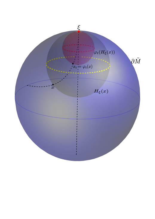
Figure 2.0. Horospheres and action of $\varphi_{t}=\varphi_{t,\xi}$

Definition 2.2 (Stable Holonomy for Horospheres).

A stable holonomy is a family of maps $(x,y,\xi)\rightarrow\Pi^{\xi}_{s}(x,y)$, $s\in\mathbb{R}$, defined on the set of points $(x,y,\xi)$ such that $x,y$ belong to the horosphere $H_{\xi}(s)$, and such that the following properties hold:

1. $\Pi^{\xi}_{s}(x,y)$ is a linear map from $T_{x}H_{\xi}(s)$ to $T_{y}H_{\xi}(s)$ for every $s\in\mathbb{R}$, $x,y\in H_{\xi}(s)$,

2. $\Pi^{\xi}_{s}(x,x)=Id$ and $\Pi^{\xi}_{s}(x,y)=\Pi^{\xi}_{s}(z,y)\circ\Pi^{\xi}_{s}(x,z)$ for every $s\in\mathbb{R}$, $x,y,z\in H_{\xi}(s)$

3. $\Pi^{\xi}_{s}(x,y)=D\varphi^{-1}_{t,\xi}(\varphi_{t,\xi}(y))\circ\Pi^{\xi}_{s+t}(\varphi_{t,\xi}(x),\varphi_{t,\xi}(y))\circ D\varphi_{t,\xi}(x)$ for all $t\in\mathbb{R}$, $s\in\mathbb{R},$

where $D\varphi_{t,\xi}(z)$ denotes the differential of $\varphi_{t,\xi}$ at the point $z$.

Notice that condition (2) tells that this stable holonomy, if it exists, is ’flat’.

Let us choose a point $\xi\in\partial\tilde{M}$. In the sequel of this section, we will set $\varphi_{t}:=\varphi_{t,\xi},t\in\mathbb{R}$ and $\tilde{p}_{\xi}=\tilde{p}$. Recall that the induced Riemannian metric on $H_{\xi}(t)$ is denoted by $h_{t}$, and let $\nabla^{t}$ denote the Levi-Civita connection associated to $h_{t}$. The parallel transport with respect to $\nabla^{t}$, along any path joining any two points $x$ and $y$ in $H_{\xi}(t)$, is an isometry between $T_{x}H_{\xi}(t)$ and $T_{y}H_{\xi}(t)$. The isometry a priori depends on the path. However, if $x,y$ in $H_{\xi}(t)$ are at distance less than the injectivity radius of $H_{\xi}(t)$, there exists a unique geodesic segment joining $x$ and $y$ and we will therefore denote by

(2.3) $$P_{t}^{\xi}(x,y)$$

the parallel transport along this segment.

We now turn to the main proposition of this section that will grant us the existence of the stable holonomy along horospheres. It is a reformulation of [12, Proposition 4.2] or of [6, Proposition 2.2]. Since we will use the construction later on, we will shortly describe it. We first need two lemmas.

The first lemma follows from the hypotheses on the curvature of $M$. Let us normalize the sectional curvature $\kappa$ of $M$, so that the following inequalities are satisfied for some constant $1>\tau>0$,

(2.4) $$-4(1-\tau)\leq\kappa\leq-1.$$

The first lemma is a consequence of this pinching condition.

Lemma 2.5.

Let $x,y$ be two points on $H_{\xi}(s)$ and let $X$ be a tangent vector in $T_{x}H_{\xi}(s)$. Then, for any $t\geq 0$, the following estimates hold

1. $\|D\varphi_{t}(x)(X)\|_{h_{s+t}}\leq e^{-t}\|X\|_{h_{s}}$,

2. $\|D\varphi_{t}^{-1}(x)(X)\|_{h_{s-t}}\leq e^{(2\sqrt{1-\tau})t}\|X\|_{h_{s}}\leq e^{(2-\tau)t}\|X\|_{h_{s}},$ and

3. $d_{h_{s+t}}(\varphi_{t}(x),\varphi_{t}(y))\leq e^{-t}d_{h_{s}}(x,y)$.

Proof.

The norm and the distance we use above is computed with respect to the induced Riemannian metric on the corresponding horosphere. Recall that a stable Jacobi field $Y(t)$ along a geodesic ray $c_{\tilde{v}}(t)$, $t>0$, is a bounded Jacobi field, see [10, Definition 2.1]. The proof of these inequalities is a direct consequence of the estimate of the growth of the stable Jacobi fields as done in [10, Theorem 2.4].

In fact, we only need to show that $D\varphi_{t}(X)$ is a stable Jacobi field. This follows from the Anosov property of the geodesic flow of $M$, see [2, Appendice 21]. Indeed, if $X$ is a tangent vector in $T_{x}H_{\xi}(s)$ at the point $x$, then $X=D\tilde{p}(\tilde{v})(V)$, where $V\in E^{ss}(\tilde{v})\subset T_{\tilde{v}}T^{1}\tilde{M}$, and $\tilde{v}$ is the unit vector in $T_{x}\tilde{M}$ perpendicular to $H_{\xi}(s)$ and pointing toward $\xi$. Therefore, by applying the chain rule to Equation (2.1), and recalling that $x={\tilde{p}}({\tilde{v}})$, we obtain that

(2.6) $$D\varphi_{t}(x)(X)=D\tilde{p}(\tilde{g}_{t}(\tilde{v}))\circ D\tilde{g}_{t}(\tilde{v})(V).$$

Since the geodesic flow of $M$ is Anosov and $V\in E^{ss}(\tilde{v})$, it follows that

(2.7) $$\lim_{t\to\infty}\|D\tilde{g}_{t}(\tilde{v})(V)\|=0,$$

which implies that $\lim_{t\to\infty}\|D\varphi_{t}(x)(X)\|=0$. Indeed the map $\tilde{p}:T^{1}\tilde{M}\rightarrow\tilde{M}$ is defined on the quotient (by $\pi_{1}(M)$) by $p:T^{1}M\rightarrow M$, the compactness of $M$ grants us that $\tilde{p}$ as well as $D\tilde{p}$ are bounded. Hence, it follows that $D\varphi_{t}(X)$ is a stable Jacobi field and this concludes the proof of the first assertion of the Lemma 2.5. The other assertions follow easily.

∎

Since $(\tilde{M},\tilde{g})$ covers the closed manifold $(M,g)$, for each $\sigma\in[0,1]$, we are able to obtain a uniform control on the action of $\varphi_{\sigma}$ as follows. We first study the behavior of the family of horospheres $H_{\xi}(s)$, $s\in\mathbb{R}$, orthogonal to the geodesic $c_{\tilde{v}}(s)$ such that $c_{\tilde{v}}(+\infty)=\xi$. By assertion (3) of Proposition 1.1, we will assume from now on that the injectivity radius of every horosphere is bounded below by $\rho>0$. For each $x\in H_{\xi}(s)$, we denote $c_{x}$ the geodesic passing through $x$ asymptotic to $\xi$, ie. $c_{x}(+\infty)=c_{\tilde{v}}(+\infty)=\xi$ parametrized in such a way that $c_{x}(s)=x$.

Lemma 2.8.

There exists a constant $C>0$ such that for any $s\in\mathbb{R}$, any $\sigma\in[0,1]$, any two points $x,y\in H_{\xi}(s)$ such that $d_{H_{\xi}(s)}(x,y)<\rho$, and any $X\in T_{x}H_{\xi}(s)$, the following holds.

(2.9) $$\|\left(D\varphi_{\sigma}^{-1}(\varphi_{\sigma}(y))\circ P^{\xi}_{s+\sigma}(\varphi_{\sigma}(x),\varphi_{\sigma}(y))\circ D\varphi_{\sigma}(x)-P^{\xi}_{s}(x,y)\right)(X)\|_{h_{s}}\leq Cd_{h_{s}}(x,y)\,\|X\|_{h_{s}}.$$

Proof.

Let us first assume that $X\in T_{x}H_{\xi}(s)$ has a unit norm. Define $X_{\sigma}:=D\varphi_{\sigma}(x)X$ and let $c:[0,d]\to H_{\xi}(s)$ be the geodesic segment of $H_{\xi}(s)$ between $x$ and $y$, where $d=d_{h_{s}}(x,y)$. Let $c_{\sigma}(u):[0,d]\longrightarrow H_{\xi}(s+\sigma),$ be the geodesic segment, parametrized with constant speed, joining $\varphi_{\sigma}(x)$ and $\varphi_{\sigma}(y)$ which exists by Lemma 2.5, (3). Notice that also by Lemma 2.5 we have

(2.10) $$e^{-(2-\tau)}\leq|\dot{c}_{\sigma}|\leq 1.$$

We have,

$$D\varphi_{\sigma}^{-1}(\varphi_{\sigma}(y))\circ P^{\xi}_{s+\sigma}(\varphi_{\sigma}(x),\varphi_{\sigma}(y))\circ D\varphi_{\sigma}(x)-P^{\xi}_{s}(x,y)=$$

$$\int_{0}^{d}\frac{d}{du}\left(D\varphi_{\sigma}^{-1}(c_{\sigma}(u))\circ\left(P^{\xi}_{s+\sigma}(\varphi_{\sigma}(x),c_{\sigma}(u))\circ D\varphi_{\sigma}(x)-D\varphi_{\sigma}(c(u))\circ P^{\xi}_{s}(x,c(u))\right)\right)du.$$

By compactness of $M$ and by (2.1), the norm of every covariant derivative of $\varphi^{\xi}_{\sigma}$ and $(\varphi^{\xi}_{\sigma})^{-1}$, $\xi\in\partial\tilde{M}$ and $\sigma\in[0,1]$ is bounded above by a constant depending on the degree of derivation. In particular, there exists a constant $C>0$ such that the integrand in the right hand side term above is bounded by a constant $C$.

We deduce that

(2.11) $$\|P^{\xi}_{s}(x,y)(X)-D\varphi_{\sigma}^{-1}(\varphi_{\sigma}(y))\circ P^{\xi}_{s+\sigma}(\varphi_{\sigma}(x),\varphi_{\sigma}(y))\circ D\varphi_{\sigma}(x)(X)\|_{h_{s}}\leq Cd_{h_{s}}(x,y).$$

If the norm of $X$ is not equal to $1$, the desired inequality follows by simple modifications of the proof above.

∎

Remark 2.12.

Notice that the constant $C$ in the above proposition does not depend on the horosphere $H_{\xi}(s)$ nor even on $\xi$. More precisely, in formula 2.11 the parallel transport operators are isometries, hence their norms are bounded by one. Only the differential of $\phi_{\sigma}$ matters. These maps, for $\sigma\in[0,1]$ are projections, by $\tilde{p}$ to $\tilde{M}$, of the geodesic flow on $T^{1}\tilde{M}$ restricted to the submanifolds $\tilde{W}^{s}(\xi)$. Now by compactness of $M$, $T^{1}(M)$ and $[0,1]$, $\tilde{p}$ and the geodesic flow on $T^{1}\tilde{M}$ have bounded derivatives at any order. Finally the arguments in Subsection 1.1 show that the manifolds $\tilde{W}^{s}(\xi)$ have uniformly bounded geometry at any order with constants independent of $\xi$.

Notice however that independence on $\xi$ is not really needed in our argument.

We now turn to prove the existence of a stable holonomy. For every $\tilde{v}\in T^{1}\tilde{M}$, we consider the family of horospheres centered at $\xi:=c_{\tilde{v}}(+\infty)$, which we parametrize as $H_{\xi}(t)$, $t\in\mathbb{R}$, where the parameter $t=0$ corresponds to the horosphere containing the base point of $\tilde{v}$.

Proposition 2.13.

Let $M$ be a closed Riemannian manifold with pinched negative curvature satisfying $-4(1-\tau)\leq\kappa\leq-1$. Let $\tilde{v}$ be a unit vector tangent to $\tilde{M}$. Let $\xi=\lim_{t\to+\infty}c_{\tilde{v}}(t)\in\partial\tilde{M}$. Then,

1. For every $s\in\mathbb{R}$, $x,y\in H_{\xi}(s)$, there exists a linear map

   $$\Pi^{\xi}_{s}(x,y):T_{x}H_{\xi}(s)\to T_{y}H_{\xi}(s)$$

   satisfying conditions (1), (2), (3) in Definition (2.2),

2. $\|\Pi^{\xi}_{s}(x,y)-P_{s}^{\xi}(x,y)\|\leq Cd_{h_{s}}(x,y)$ for all $x,y$ such that $d_{h_{s}}(x,y)<\rho$.

3. Properties (i) and (ii) uniquely determine the stable holonomy.

4. The stable holonomy is $\pi_{1}(M)$-equivariant, ie for every $\gamma\in\pi_{1}(M)$, we have

   $$\Pi^{\gamma\xi}_{s}(\gamma x,\gamma y)=\gamma_{*}\circ\Pi^{\xi}_{s}(x,y).$$

Proof.

The proof follows closely the methods given in [12, Proposition 4.2]. We reproduce here only the part of the construction, modified to our setting, which we will need in the sequel. Let us consider $x,y\in H_{\xi}(s)$ such that $d_{H_{\xi}(s)}(x,y)\leq R$, for some fixed $R$. For every $x\in H_{\xi}(s)$, denote $x_{t}:=\varphi_{t}(x)\in H_{\xi}(s+t)$. By Lemma 2.5 (3), there exists $t_{0}:=t_{0}(R)\geq 0$ such that $d_{H_{\xi}(s+t_{0})}(x_{t_{0}},y_{t_{0}})<\rho$.

Let us turn to proving assertion (i). For every $t\in\mathbb{R}$, define

$$c_{t}:[0,1]\to H_{\xi}(s+t)$$

the geodesic segment, parametrized with constant speed, between $x_{t}$ and $y_{t}$ which is well defined when their distance is less than $\rho$.

For $x,y\in H_{\xi}(s)$ we define

(2.14) $$\Pi^{\xi}_{s}(x,y)=\lim_{t\to\infty}d\varphi_{t}^{-1}(y_{t})\circ P^{\xi}_{t}(x_{t},y_{t})\circ d\varphi_{t}(x).$$

Notice that the above term $P^{\xi}_{t}(x_{t},y_{t})$ in the limit is well defined for all $t\geq t_{0}$ since the distance between $x_{t}$ and $y_{t}$ is decreasing. Let us show that the above limit exists. Define for $j\geq 0$, $x,y\in H_{\xi}(s)$,

$$\Pi^{\xi}_{s,j}(x,y):=d\varphi_{t_{0}+j}^{-1}(y_{t_{0}+j})\circ P^{\xi}_{s+t_{0}+j}(x_{t_{0}+j},y_{t_{0}+j})\circ d\varphi_{t_{0}+j}(x).$$

We have for every $N\geq 0$,

(2.15) $$\Pi^{\xi}_{s,N}(x,y)=\Pi^{\xi}_{s,0}(x,y)+\sum_{j=0}^{N-1}\left(\Pi^{\xi}_{s,j+1}(x,y)-\Pi^{\xi}_{s,j}(x,y)\right).$$

Each term in the above sum is expanded as

$$\left(\Pi_{s,j+1}^{\xi}-\Pi_{s,j}^{\xi}\right)(x,y)=$$

$$D\varphi_{t_{0}+j}^{-1}(y_{t_{0}+j})\circ\big{[}D\varphi_{1}^{-1}(y_{t_{0}+j+1})\circ P^{\xi}_{s+t_{0}+j+1}(x_{t_{0}+j+1},y_{t_{0}+j+1})\circ D\varphi_{1}(x_{t_{0}+j})-P_{c_{j}}(x_{t_{0}+j},y_{t_{0}+j})\big{]}\circ D\varphi_{t_{0}+j}(x),$$

hence, by Lemma 2.8, we get

(2.16) $$\|\left(\Pi_{s,j+1}^{\xi}-\Pi_{s,j}^{\xi}\right)(x,y)\|\leq C\|D\varphi_{t_{0}+j}^{-1}(y_{t_{0}+j})\|\|D\varphi_{t_{0}+j}(x)\|d_{h_{s+t_{0}+j}}(x_{t_{0}+j},y_{t_{0}+j}).$$

Assertion (3) of Lemma 2.5 implies that

(2.17) $$d_{h_{t_{0}+s+j}}(x_{t_{0}+j},y_{t_{0}+j})\leq e^{-{(t_{0}+j)}}d_{h_{s}}(x,y)$$

and substituting back in (2.16) yield that

(2.18) $$\|\left(\Pi_{s,j+1}^{\xi}-\Pi_{s,j}^{\xi}\right)(x,y)\|\leq Ce^{-\tau(t_{0}+j)}d_{h_{s}}(x,y).$$

Therefore, the limit in (2.14) exists and is well defined. The $\pi_{1}(M)$-invariance is obvious and proofs of the others parts of this proposition are the same as in those of Theorem 4.2 of [12].

∎

Remark 2.19.

In the proof of the above proposition, the following fact, which will be useful later, was under the lines.

Claim 2.20.

For every $\epsilon>0$, and $d>0$, there exists $N$ such that for every $\xi\in\partial\tilde{M}$, every pair of points in a horosphere $H_{\xi}$ such that $d_{H_{\xi}}(x,y)\leq d$, then

$$\|\Pi^{\xi}(x,y)-\Pi^{\xi}_{N}(x,y)\|\leq\epsilon,$$

where $\Pi^{\xi}_{N}(x,y)$ is defined in (2.15) with $s=0$.

Let us prove the claim. By (2.15)

$$\Pi^{\xi}(x,y)-\Pi^{\xi}_{N}(x,y)=\sum_{j=N}^{\infty}\left(\Pi^{\xi}_{j+1}(x,y)-\Pi^{\xi}_{j}(x,y)\right).$$

and by (2.18)

$$\|\Pi^{\xi}(x,y)-\Pi^{\xi}_{N}(x,y)\|\leq C\sum_{j=N}^{\infty}e^{-\tau(t_{0}+j)}d_{h_{s}}(x,y),$$

which concludes the proof of the claim since the rest of the series satisfies

$$\sum_{j=N}^{\infty}e^{-\tau(t_{0}+j)}d_{h_{s}}(x,y)\leq d\sum_{j=N}^{\infty}e^{-j\tau}\leq\epsilon$$

for $N$ large enough.

We now wish to compare the stable holonomy with the parallel transport of the Levi-Civita connection on horospheres. Consider two points $x,y$ on a horosphere $H_{\xi}$ in $\tilde{M}$ centered at $\xi\in\partial\tilde{M}$. Assume that $d_{H_{\xi}}(x,y)<\rho$ is smaller than the injectivity radius of $H_{\xi}$. We recall that, by Proposition 1.1 (3), the injectivity radius of every horosphere is bounded below by a constant $\rho>0$. The stable holonomy $\Pi^{\xi}(x,y)$ and the parallel transport $P^{\xi}(x,y)$ along the unique geodesic segment joining $x$ and $y$ a priori do not coincide. We insist on the fact that the stable holonomy is a dynamical object whereas the Levi-Civita connection is geometric. Assuming that they coincide locally on a horosphere has the following strong implication.

Proposition 2.21.

Let $M$ be a closed Riemannian manifold with pinched negative curvature satisfying $-4(1-\tau)\leq\kappa\leq-1$. Let $\xi$ be a point in $\partial\tilde{M}$ and $x_{0}\in H_{\xi}$ be a point in a horosphere centered at $\xi$. Assume that for every $x,y\in B_{H_{\xi}}(x_{0},\frac{\rho}{2})$, the stable holonomy $\Pi^{\xi}(x,y)$ coincide with the parallel transport $P^{\xi}(x,y)$ of the Levi-Civita connection of $H_{\xi}$. Then the induced metric on $H_{\xi}$ restricted to $B_{H_{\xi}}(x_{0},\frac{\rho}{2})$ is flat.

Proof.

Since any pair of points in $B_{H_{\xi}}(x_{0},\frac{\rho}{2})$ are at distance less than $\rho$, there is a unique geodesic segment joining them and by our coincidence assumption and assertion (2) of 2.2 it follows that

$$P^{\xi}(x,y)=P^{\xi}(z,y)\circ P^{\xi}(x,z).$$

From the classical formula of the curvature in terms of the parallel transport, see for instance [14, Theorem 7.1], we deduce that the curvature of the induced metric of $H_{\xi}$ restricted to $B_{H_{\xi}}(x_{0},\frac{\rho}{2})$ is identically zero.

∎

The goal of what follows is to show that if the stable holonomy and the parallel transport of the Levi-Civita connection locally coincide on a given horosphere $H_{\xi}$, then the same property holds on all horospheres. To accomplish this, we need to establish the continuity of the stable holonomy. Let $\tilde{v}$ be a unit vector tangent to $\tilde{M}$ and $\tilde{v}_{k}\in T^{1}\tilde{M}$ a sequence of unit tangent vectors such that $\lim_{k}\tilde{v}_{k}=\tilde{v}$. Let $\xi_{\tilde{v}}=c_{\tilde{v}}(+\infty)$ the associated point on $\partial\tilde{M}$. Denote by $H_{\tilde{v}}$ be the horosphere centered at $\xi_{\tilde{v}}$ passing through the base point of $\tilde{v}$. Let $\tilde{Q}_{k}$ and $\tilde{Q}$ the lifts of the plaques $Q_{k}$ and $Q$ of the strong stable foliation $W^{ss}$ embedded in a chart $U\subset T^{1}M$ and containing $\tilde{v}_{k}$ and $\tilde{v}$ respectively. Recall that, from Proposition 1.1, the sequence of diffeomorphisms

(2.22) $$\pi^{-1}\circ p\circ\Theta(v_{k}):D^{n}\to\tilde{p}(\tilde{Q}_{k})$$

converges in the $C^{r}$-topology to

(2.23) $$\pi^{-1}\circ p\circ\Theta(v):D^{n}\to\tilde{p}(\tilde{Q}).$$

Proposition 2.24.

Let $\tilde{v}_{k}\in T^{1}\tilde{M}$ be a sequence of unit tangent vectors such that $\lim_{k}\tilde{v}_{k}=\tilde{v}$.

Let $x=\pi^{-1}\circ p\circ\Theta(v)(q_{x})$, $y=\pi^{-1}\circ p\circ\Theta(v)\mathcal{(}q_{y})$ be a pair of point in $\tilde{p}(\tilde{Q})$ and $x_{k}=\pi^{-1}\circ p\circ\Theta(v_{k})(q_{x_{k}})$, $y_{k}=\pi^{-1}\circ p\circ\Theta(v_{k})(q_{y_{k}})$ in $\tilde{p}(\tilde{Q}_{k})$. Then

$$\lim_{k}\Pi^{\xi_{\tilde{v}_{k}}}(x_{k},y_{k})=\Pi^{\xi_{v}}(x,y).$$

Proof.

Let us fix $\epsilon>0$. By the claim 2.20, we can choose $N$ such that for every $x,y\in\tilde{p}(\tilde{Q})$ and every $x_{k},y_{k}\in\tilde{p}(\tilde{Q}_{k})$, we have

(2.25) $$||\Pi^{\xi_{\tilde{v}}}(x,y)-\Pi^{\xi_{\tilde{v}}}_{N}(x,y)||\leq\epsilon$$

and similarly,

(2.26) $$||\Pi^{\xi_{\tilde{v}_{k}}}(x_{k},y_{k})-\Pi^{\xi_{\tilde{v}_{k}}}_{N}(x_{k},y_{k})||\leq\epsilon.$$

By the above convergence of (2.22 ) to (2.23), the points $x_{k}$ and $y_{k}$ converge to $x$ and $y$ and the unit normals to $\tilde{p}(\tilde{Q}_{k})$ at $x_{k}$ and $y_{k}$ converge to the unit normals to $\tilde{p}(\tilde{Q})$ at $x$ and $y$, respectively. Therefore the flows $(\varphi^{\xi_{\tilde{v}_{k}}}_{t})_{|\tilde{p}(\tilde{Q}_{k})}$ converge to $(\varphi^{\xi_{\tilde{v}}}_{t})_{|\tilde{p}(\tilde{Q})}$ uniformly for $t\in[0,T]$ for every $T$. Now, the way $\Pi^{\xi_{\tilde{v}}}_{N}(x,y)$ depends on $\varphi^{\xi_{\tilde{v}}}_{t}$, $t\leq N$ and the fact that $t_{0}\leq\log\rho$ implies that $\Pi^{\xi_{\tilde{v}_{k}}}_{N}(x_{k},y_{k})$ converges to $\Pi^{\xi_{\tilde{v}}}_{N}(x,y)$. Therefore, there exists $K>0$ such that for all $k\geq K$,

$$\|\Pi^{\xi_{\tilde{v}}}_{N}(x,y)-\Pi^{\xi_{\tilde{v}_{k}}}_{N}(x_{k},y_{k})\|\leq\epsilon.$$

We then deduce that for $N$ and $k\geq K$,

$$\|\Pi^{\xi_{\tilde{v}}}(x,y)-\Pi^{\xi_{\tilde{v}_{k}}}(x_{k},y_{k})\|\leq$$

$$\|\Pi^{\xi_{\tilde{v}}}(x,y)-\Pi^{\xi_{\tilde{v}}}_{N}(x,y)\|+\|\Pi^{\xi_{\tilde{v}}}_{N}(x,y)-\Pi^{\xi_{\tilde{v}_{k}}}_{N}(x_{k},y_{k})\|+\|\Pi^{\xi_{\tilde{v}_{k}}}_{N}(x_{k},y_{k})-\Pi^{\xi_{\tilde{v}_{k}}}(x_{k},y_{k})\|$$

thus, $\|\Pi^{\xi_{\tilde{v}}}(x,y)-\Pi^{\xi_{\tilde{v}_{k}}}(x_{k},y_{k})\|\leq 3\epsilon$, which concludes the proof.

∎

We can now state the main result of this section.

Proposition 2.27.

Let $M$ be a closed Riemannian manifold with pinched negative curvature satisfying $-4(1-\tau)\leq\kappa\leq-1$. Let $\tilde{v}$ be a unit tangent vector in $T^{1}\tilde{M}$ and $\xi_{\tilde{v}}=c_{\tilde{v}}(+\infty)$ the corresponding point in $\partial\tilde{M}$. Assume that the stable holonomy $\Pi^{\xi_{\tilde{v}}}(x,y)$ and the parallel transport for the Levi-Civita connection $P^{\xi_{\tilde{v}}}(x,y)$ coincide on every ball of radius $\rho/2$ of the horosphere $H_{\xi_{\tilde{v}}}$. Then for every horosphere $H_{\xi_{\tilde{w}}}$, $\tilde{w}\in T^{1}\tilde{M}$, and every $z\in H_{\xi_{\tilde{w}}}$, there exists a neighbourhood $\mathcal{V}(z)\subset H_{\xi_{\tilde{w}}}$ of $z$ such that the stable holonomy $\Pi^{\xi_{\tilde{v}}}(x,y)$ and the parallel transport for the Levi-Civita connection $P^{\xi_{\tilde{v}}}(x,y)$ coincide for all points $x,y\in\mathcal{V}(z)$.

Proof.

Suppose that $H_{\tilde{v}}$ satisfies the assumption of the proposition and let us consider a different horosphere $H_{\tilde{w}}$. We will prove that locally around $\tilde{p}(\tilde{w})$ on $H_{\tilde{w}}$, the stable holonomy and the Levi-Civita parallel transport coincide. As mentioned in the proof of assertion (2) in Proposition 1.1, each leaf of the strong stable foliation $W^{ss}\subset T^{1}M$, in particular $W^{ss}(v)$, is dense in $T^{1}M$, where $v=d\tilde{\pi}(\tilde{v})$. Moreover, thanks to (1.6) and (1.7) in Proposition 1.1, the lift $\tilde{p}(\tilde{Q})\subset H_{\tilde{w}}$ is the $C^{r}$ limit of the sequence of sets $\tilde{p}(\tilde{Q}_{l})$ where $\tilde{Q}_{l}$ are lifts of $Q_{l}$. These lifts $\tilde{Q}_{l}$ are subsets of translates, by elements of the fundamental group of $M$, of $H_{\tilde{v}}$. By the $\pi_{1}(M)$-equivariance of the stable holonomy (coming from Proposition 2.13) and of the Levi-Civita connection, we get from our assumption that the stable holonomy and the parallel transport of the Levi-Civita connection coincide on $\tilde{p}(\tilde{Q}_{l})$. The proof then follows from the continuity properties of Proposition 2.24 and Proposition 1.1 (4).

∎

Corollary 2.28.

Let $M$ be a closed Riemannian manifold with pinched negative curvature satisfying $-4(1-\tau)\leq\kappa\leq-1$. If the stable holonomy and the parallel transport of the induced Levi-Civita connection coincide on every ball of radius $\rho/2$ of one horosphere $H_{\xi_{\tilde{v}}}$, then the induced metric on each horosphere of $\tilde{M}$ is isometric to a Euclidean metric. Moreover, for every $\tilde{w}\in T^{1}\tilde{M}$, $x,y\in H_{\xi_{\tilde{w}}}$ we have $\Pi^{\xi_{\tilde{w}}}_{s}(x,y)=P^{\xi_{\tilde{w}}}_{s}(x,y)$, in other words, the stable holonomy and the parallel transport associated to the Euclidean metric coincide on every horosphere. In particular, the parallel transport associated to the Euclidean metric is invariant by the geodeisc flow.

Proof.

By the Proposition 2.27, for every horosphere $H_{\xi_{\tilde{w}}}$ and $x\in H_{\xi_{\tilde{w}}}$, the stable holonomy and the parallel transport associated to the Levi-Civita connexion coincide on a neighbouhood $\mathcal{V}(x)$ of $x$. Thanks to the proposition 2.21 applied to $\mathcal{V}(x)$, we deduce that the induced metric on every horosphere has a flat Levi-Civita connexion, hence is a Euclidean metric. This proves the first part. Let us prove the second part of the Corollary. Let us consider $x,y\in H_{\xi_{\tilde{w}}}$. Choose a continuous path $c:[0,1]\to H_{\xi_{\tilde{w}}}$ such that $c(0)=x$ and $c(1)=y$. There exists $t_{0}=0<t_{1}<...<t_{2k}=1$ such that $\{\mathcal{V}(c(t_{2i}))\}_{i=0}^{k}$ is a finite covering of $c([0,1])$ and $c(t_{2i+1})\in\mathcal{V}(c(t_{2i}))\cap\mathcal{V}(c(t_{2(i+1)}))$. Since the Levi-Civita connexion on the metric of $H_{\xi_{\tilde{w}}}$ is flat we have,

$$P^{\xi_{\tilde{w}}}_{s}(x,y)=P^{\xi_{\tilde{w}}}_{s}(c(t_{0}),c(t_{1}))\circ P^{\xi_{\tilde{w}}}_{s}(c(t_{1},c(t_{2}))\circ.....\circ P^{\xi_{\tilde{w}}}_{s}(c(t_{2k-1},c(t_{2k}))$$

and similarly, thanks to the property (2) of the definition 2.2,

$$\Pi^{\xi_{\tilde{w}}}_{s}(x,y)=\Pi^{\xi_{\tilde{w}}}_{s}(c(t_{0}),c(t_{1}))\circ\Pi^{\xi_{\tilde{w}}}_{s}(c(t_{1},c(t_{2}))\circ.....\circ\Pi^{\xi_{\tilde{w}}}_{s}(c(t_{2k-1},c(t_{2k})).$$

We then conclude that $P^{\xi_{\tilde{w}}}_{s}(x,y)=\Pi^{\xi_{\tilde{w}}}_{s}(x,y)$ since $P^{\xi_{\tilde{w}}}_{s}(c(t_{j}),c(t_{j+1}))=\Pi^{\xi_{\tilde{w}}}_{s}(c(t_{j}),c(t_{j+1}))$.

∎

3. A quasi-isometry between $\tilde{M}$ and a Heintze group

In this section, the main theorem of this article, Theorem 0.2, will be proved. As we explained in the introduction, the proof amounts to proving Theorem 0.4. Henceforth, $M$ is assumed to be a closed, strictly quarter-pinched, negatively curved Riemannian manifold of dimension greater than or equal to $3$. Furthermore, by Corollary 2.27 we may assume that all the horospheres in $\tilde{M}$ are isometric to the Euclidean space and that the associated parallel transport is invariant by the geodesic flow. We will therefore be able to prove below the following. Given a geodesic $c_{\tilde{v}}(t)$ in $\tilde{M}$ which projects to a closed geodesic in $M$, there exists a quasi-isometry between the universal cover $\tilde{M}$ of $M$ and the Heintze group $G_{A}$, where $A$ is the derivative of the first return Poincaré map along the closed geodesic. Theorem 0.5, will then imply that the eigenvalues of $A$ all have the same modulus, hence concluding the proof of Theorem 0.4.

Let us choose a geodesic $c_{\tilde{v}}(t)$ in $\tilde{M}$ with end point $\xi=c_{\tilde{v}}(\infty)\in\partial\tilde{M}$, which projects to a closed geodesic in $M$. We consider the horosphere $H_{\xi}(0)$ centred at $\xi$ and passing through the base point $x_{0}=c_{\tilde{v}}(0)$. For each $p\in\tilde{M}$, the geodesic $c$ joining $p$ and $\xi$ intersects $H_{\xi}(0)$ at a point $x=c(0)$. The pair, $(t,x)\in\mathbb{R}\times H_{\xi}(0)$, are the horospherical coordinates of $p$.

Keeping the same notation as in Section 2, we recall that $\{\varphi_{t}\}_{t\in\mathbb{R}}$ is a one parameter group of diffeomorphisms of $\tilde{M}$ which sends $H_{\xi}(0)$ diffeomorphically onto $H_{\xi}(t)$ (see 2.1) and the above horospherical coordinates realise the following diffeomorphism $\Phi:\mathbb{R}\times H_{\xi}(0)\rightarrow\tilde{M}$ defined by

(3.1) $$(t,x)\rightarrow\varphi_{t}(x),\text{ for }t\in\mathbb{R}\text{ and }x\in H_{\xi}(0).$$

Therefore, in horospherical coordinates, the pulled back by $\Phi$ of the metric $\tilde{g}$ on $\tilde{M}$ at $(t,x)$ writes as the orthogonal sum:

(3.2) $$\Phi^{*}(\tilde{g})=dt^{2}+\varphi_{t}^{*}h_{t}(x),$$

where $\varphi_{t}^{*}h_{t}$ is a flat metric on $H_{\xi}(0)$. Note that $\varphi_{t}$ acts by translation on geodesics, hence, there is no effect on the $dt^{2}$ factor.

As before, since the horosphere $(H_{\xi}(0),h_{0})$ is flat we will identify it with the Euclidean space $(\mathbb{R}^{n},h_{\mathrm{eucl}})$. The geodesic $c_{\tilde{v}}$ projects to a closed geodesic on $M$ of period $l$. Let $\gamma$ be the element of the fundamental group of $M$ with axis $c_{\tilde{v}}$ such that $D\gamma(\tilde{g}_{l}(\tilde{v}))=\tilde{v}$. The map $\psi=\gamma\circ\varphi_{l}$ is a diffeomorphism of $\tilde{M}$, (see definition 3.5 below). When restricted to $H_{\xi}(0)$, $\psi$ can be considered as a diffeomorphism of $\mathbb{R}^{n}$ fixing $x_{0}$, and $d\psi(x_{0})$ as a linear operator of $\mathbb{R}^{n}$ which we will denote by $T$, see the definitions 3.5 and 3.7 below, where $T=T^{1}$. Up to replacing $T$ by $T^{2}$, we can assume that $T$ is contained in a one parameter group in $GL(n,\mathbb{R})$, i.e. $T=e^{lA}$ for some matrix $A$ (see [7]). Indeed, replacing $T$ with $T^{2}=D\psi(x_{0})^{2}$, we simply work with twice the periodic orbit of period $2l$ and the argument is rigorously the same. We thus can assume from now on that $T=e^{lA}$. Let us consider the Heintze group $G_{A}$ associated to the matrix $A$ and recall from Section 1 that

$G_{A}=\mathbb{R}\ltimes_{A}\mathbb{R}^{n}$ is the solvable group endowed with the multiplication law

(3.3) $$(s,x)\cdot(t,y)=(s+t,x+e^{-sA}y),\text{ for all }s,t\in\mathbb{R},x,y\in\mathbb{R}^{n}.$$

The group $G_{A}$ is diffeomorphic to $\mathbb{R}\times\mathbb{R}^{n}$, and the tangent space at each point $(s,x)$ of $G_{A}$ splits as $\mathbb{R}\times\mathbb{R}^{n}$. Let us consider the left invariant metric $g_{A}$ on $G_{A}$ which is defined to be the standard Euclidean metric at $(0,0)\in G_{A}$, where $\mathbb{R}\times\{0\}$ is orthogonal to $\{0\}\times\mathbb{R}^{n}$. Since the inverse of the left multiplication is given by $L_{(s,x)^{-1}}(t,y)=(t-s,-e^{sA}x+e^{sA}y)$, an easy computation shows that the metric $g_{A}$ is then defined, for a vector $Z=(a,X)$ which is tangent to $G_{A}$ at an arbitrary point $(s,x)\in G_{A}$, by

(3.4) $$g_{A}(s,x)(Z,Z)=a^{2}+h_{\mathrm{eucl}}(e^{sA}X,e^{sA}X).$$

We start by identifying the flat horosphere ($H_{\xi}(0),h_{0})$ with the Euclidean space $(\mathbb{R}^{n},d_{\mathrm{eucl}})$. Let us recall that $c_{\tilde{v}}$ is a geodesic in $\tilde{M}$ with $\xi=c_{\tilde{v}}(\infty)\in\partial\tilde{M}$, which projects to a closed geodesic in $M$ of period $l$. We do not require that this geodesic is primitive; in fact, we will later replace the corresponding element $\gamma$ of the fundamental group by a large enough power of it.

We now consider the diffeomorphism of $H_{\xi}(0)$ defined by

(3.5) $$\psi(x)=\gamma\circ\varphi_{l}(x),\ \text{for }x\in H_{\xi}(0).$$

For all $k\geq 1$, let $\psi^{k}=\psi\circ\psi\dots\circ\psi$ denote the $k$-th power of $\psi$. For $x\in H_{\xi}(0)$, we define

(3.6) $$T_{k}(x)=d\psi\left(\psi^{k-1}(x)\right),$$

and

(3.7) $$T^{k}(x)=T_{k}(x)\cdot T_{k-1}(x)\cdots T_{1}(x).$$

Figure 3.0. The action of $\psi$ on horospheres.

Since $\gamma$ and $\varphi_{t}$ commute for all $t\in\mathbb{R}$, it follows that

(3.8) $$\psi^{k}(x)=\gamma^{k}\circ\varphi_{kl}(x)\text{ and }T^{k}(x)=D\psi^{k}(x)=D\gamma^{k}\circ D\varphi_{kl}(x).$$

As explained at the beginning of the section, we recall that $T^{1}(x_{0})=e^{A}$ for $A$ being a $(n\times n)$-matrix. In particular,

(3.9) $$T^{k}(x_{0})=D\psi^{k}(x_{0})=D\gamma^{k}\circ D\varphi_{kl}(x_{0})=e^{lkA}.$$

The main result of this section is the following:

Theorem 3.10.

With the notation above, $(\tilde{M},\tilde{g})$ is bi-Lipschitz diffeomorphic, hence quasi-isometric, to $(G_{A},g_{A})$.

Proof. In fact, we will show that there is a bi-Lipschitz diffeomorphism between $G_{A}$ and $\tilde{M}$. Recall that the map $\Phi:\mathbb{R}\times H_{\xi}(0)\rightarrow\tilde{M}$ defined by $\Phi(s,x)=\varphi_{s}(x)$ is a diffeomorphism.

By Corollary 2.28, the horosphere $H_{\xi}(0)$ endowed with the induced metric from $\tilde{M}$ is flat, hence, $\mathbb{R}\times H_{\xi}(0)=\mathbb{R}\times\mathbb{R}^{n}$ and therefore we can see $\Phi$ as a diffeomorphism between $G_{A}$ and $\tilde{M}$.

We first show that the two metrics $\Phi^{*}\tilde{g}$ and $g_{A}$ coincide at points with coordinates $(lk,y)$ where $k$ is an integer.

Lemma 3.11.

For every $k\in\mathbb{Z}$ and $y\in\mathbb{R}^{n}$, we have $\Phi^{*}\tilde{g}(lk,y)=g_{A}(lk,y)$.

Proof. It is clear that for tangent vectors of the form $Z=(a,0)$, we have $\tilde{g}(Z,Z)=g_{A}(Z,Z)=a^{2}$ at any point of coordinate $(t,x)$. Therefore, we now focus on tangent vectors of the type $Z=(0,X)$, where $X\in\mathbb{R}^{n}$ is a vector tangent to $H_{\xi}(0)=\mathbb{R}^{n}$ at $x$. By (3.4), it suffices to show that

(3.12) $$\Phi^{*}\tilde{g}(lk,x)(Z,Z)=h_{\mathrm{eucl}}(e^{lkA}X,e^{lkA}X).$$

In fact, it follows from (3.2) that

(3.13) $$\Phi^{*}\tilde{g}(lk,x)(Z,Z)=h_{lk}(d\varphi_{lk}(X),d\varphi_{lk}(X)),$$

where $d\varphi_{lk}(X)$ is a vector tangent to $H_{\xi}(lk)$ at $x_{lk}=\varphi_{lk}(x)$, and $h_{lk}$ is the flat metric of $H_{\xi}(lk)$. Note that the tangent vector $X$ can be extended to a constant vector field on $\mathbb{R}^{n}$, which we will still denote by $X$.

Recall (see Section 2 that for each integer $k$, $P_{lk}^{\xi}$ is the parallel transport associated to the flat metric $h_{lk}$ on $H_{\xi}(lk)$, and that $x_{0}=c_{v}(0)$ is the unique point on $H_{\xi}(0)$ which lies on the axis of $\gamma$. Let us denote by $q_{lk}$ the point $\varphi_{lk}(x_{0})$. We thus have

(3.14) $$h_{lk}(d\varphi_{lk}(X),d\varphi_{lk}(X))=h_{lk}\left(P_{lk}^{\xi}(x_{lk},q_{lk})(d\varphi_{lk}(X)),P_{lk}^{\xi}(x_{lk},q_{lk})(d\varphi_{lk}(X))\right).$$

By assumption (ii) of Theorem 0.2, the parallel transport of the flat metric $h_{0}=h_{eucl}$ ($h_{lk}$) coincides with the stable holonomy $\Pi_{0}^{\xi}$ ($\Pi_{lk}^{\xi}$) . In particular, the commutation property (3) of the Definition 2.2 holds:

(3.15) $$d\varphi_{lk}(x_{0})\circ P^{\xi}_{0}(x,x_{0})(X)=P_{lk}^{\xi}(x_{lk},q_{lk})(d\varphi_{lk}(X)).$$

Note that (3.15) relies on the fact that the family of parallel transports of the Levi-Civita connections coincide with the stable holonomies, hence is invariant by the geodesic flow and that it is the only place in the proof where we use it. We now deduce from (3.15) that

(3.16) $$h_{lk}(d\varphi_{lk}(X),d\varphi_{lk}(X))=h_{lk}\left(d\varphi_{lk}(x_{0})\circ P^{\xi}_{0}(x,x_{0})(X),d\varphi_{lk}(x_{0})\circ P^{\xi}_{0}(x,x_{0})(X)\right).$$

Since for every $k$, $\gamma^{k}$ is an isometry we obtain

(3.17) $$h_{lk}(d\varphi_{lk}(X),d\varphi_{lk}(X))=h_{0}\left(d\gamma^{k}\circ d\varphi_{lk}(x_{0})(P^{\xi}_{0}(x,x_{0})(X)),d\gamma^{k}\circ d\varphi_{lk}(x_{0})(P^{\xi}_{0}(x,x_{0})(X))\right),$$

thus, by (3.9),

(3.18) $$h_{lk}(d\varphi_{lk}(X),d\varphi_{lk}(X))=h_{0}\left(e^{lkA}(P^{\xi}_{0}(x,x_{0})(X)),e^{lkA}(P^{\xi}_{0}(x,x_{0})(X))\right).$$

Since $H_{\xi}(0)$ with the induced metric from $\tilde{M}$ is identified with $\mathbb{R}^{n}$, $h_{0}$ with the standard Euclidean metric $h_{\mathrm{eucl}}$ and $X$ is a constant vector field, we have $P^{\xi}_{0}(x,x_{0})(X)=X$ and

(3.19) $$h_{0}\left(e^{lkA}\left(P^{\xi}_{0}(x,x_{0})(X)\right),e^{lkA}\left(P^{\xi}_{0}(x,x_{0})(X)\right)\right)=h_{\mathrm{eucl}}(e^{lkA}X,e^{lkA}X),$$

which implies by (3.13) and (3.18) that

(3.20) $$\Phi^{*}\tilde{g}(lk,x)(Z,Z)=h_{\mathrm{eucl}}(e^{lkA}X,e^{lkA}X)=g_{A}(lk,x)(Z,Z),$$

which completes the proof of Lemma 3.11.

Lemma 3.11

For $t\in\mathbb{R}$, let $k$ be the integer part of $t/l$. We now compare $g_{A}(t,x)$ and $g_{A}(lk,x)$ at any $x\in\mathbb{R}^{n}$. Let us set $\sigma=\frac{t}{l}-k$ with $\sigma\in[0,1[$. For $Z=(0,X)$, we have

(3.21) $$g_{A}(t,x)(Z,Z)=h_{\mathrm{eucl}}(e^{tA}X,e^{tA}X)=h_{\mathrm{eucl}}(e^{l\sigma A}e^{lkA}X,e^{l\sigma A}e^{lkA}X)\,.$$

Recall that $e^{lA}=D(\gamma\circ\varphi_{l})(x_{0})=D\psi(x_{0})$ is a fixed $n\times n$ matrix, so that there exists a constant $C$ such that $\|e^{\pm l\sigma A}\|^{2}\leq C$ for every $\sigma\in[0,1[$. Therefore, we deduce from (3.21)

(3.22) $$C^{-1}g_{A}(lk,x)\leq g_{A}(t,x)\leq Cg_{A}(lk,x),$$

for every $lk\leq t<(k+1)l$. On the other hand, we have

$$h_{t}(D\varphi_{t}X,D\varphi_{t}X)=h_{t}(D\varphi_{l\sigma}\circ D\varphi_{lk}X,d\varphi_{l\sigma}\circ D\varphi_{lk}X)$$

and the same argument as before yields,

(3.23) $$C^{-1}\Phi^{*}\tilde{g}(lk,x)\leq\Phi^{*}\tilde{g}(t,x)\leq C\Phi^{*}\tilde{g}(lk,x)\,.$$

Then the relations (3.22), (3.23) and Lemma 3.11 conclude the proof of Theorem 3.10.

Theorem 3.10

Corollary 3.24.

All the eigenvalues of $T=D\psi(x_{0})$ have the same modulus.

Proof.

By Theorem 3.10, $(G_{A},g_{A})$ is quasi-isometric to $(\tilde{M},\tilde{g})$. Since $M$ is closed, $(\tilde{M},\tilde{g})$ is quasi-isometric to the finitely generated group $\pi_{1}(M)$ endowed with the word metric, which is therefore a hyperbolic group. We thus deduce that $G_{A}$ is quasi-isometric to a hyperbolic group and by the theorem 0.5, this can occur only if the real part of the complex eigenvalues of $A$ are equal. Recall that $A$ has been chosen so that either $T=e^{lA}$ or $T^{2}=e^{lA}$, where $T=D\psi(x_{0})$. We deduce that the eigenvalues of $T$ have the same modulus.

∎

We are now in position to prove Theorem 0.4, thus, completing the proof of Theorem 0.2.

Proof of Theorem 0.4.

Theorem 3.10 holds for any choice of a closed geodesic, or equivalently of an element $\gamma$ of the fundamental group of $M$, and so does Corollary 3.24. This implies that for any such choice, the moduli of the complex eigenvalues of $T=D\psi(x_{0})$ coincide.

Recall that

(3.25) $$D\psi(x_{0})=e^{l(v)A}=D\tilde{p}\,\circ\left(D(\gamma\circ\tilde{g}_{l(v)}(\tilde{v})|E^{ss}(\tilde{v})\right)\circ D\tilde{p}^{-1},$$

so that $Dg_{l(v)}|E^{ss}$ and $D\psi(x_{0})$ are conjugate matrices, therefore we conclude that the eigenvalues of $Dg_{l(v)}|E^{ss}$ have the same modulus.

∎

References

- [1] D. V. Anosov. Geodesic flows on closed Riemannian manifolds of negative curvature. Trudy Mat. Inst. Steklov., 90:209, 1967.
- [2] V. I. Arnold and A. Avez. Problèmes ergodiques de la mécanique classique. Monographies Internationales de Mathématiques Modernes, No. 9. Gauthier-Villars, Éditeur, Paris, 1967.
- [3] A. Avila, J. Santamaria, and M. Viana. Holonomy invariance: rough regularity and applications to Lyapunov exponents. Astérisque, (358):13–74, 2013.
- [4] P. Foulon and F. Labourie, Invent. Math. 109, No. 1, 97–111, 1992.
- [5] G. Besson, G. Courtois, and S. Gallot. Entropies et rigidités des espaces localement symétriques de courbure strictement négative. Geom. Funct. Anal., 5(5):731–799, 1995.
- [6] C. Butler. Rigidity of equality of Lyapunov exponents for geodesic flows. J. Differential Geometry, 109:39–79, 2018.
- [7] W.J. Culver. On the existence and uniqueness of the real logarithm of a matrix. Proc. Am. Math. Soc., 17:1146–1151, 1966.
- [8] E. Heintze. Compact quotients of homogeneous negatively curved riemannian manifolds. Math. Z., 140:79–80, 1974.
- [9] E. Heintze. On homogeneous manifolds of negative curvature. Math. Ann., 211:23–34, 1974.
- [10] E. Heintze and H. Christoph Im Hof. Geometry of horospheres. J. Differ. Geom., 12:481–491, 1977.
- [11] M. W. Hirsch and C. C. Pugh. Smoothness of horocycle foliations. J. Differential Geometry, 10:225–238, 1975.
- [12] B. Kalinin and V. Sadovskaya. Cocycles with one exponent over partially hyperbolic systems. Geom. Dedicata, 167:167–188, 2013.
- [13] M. Kanai. Differential-geometric studies on dynamics of geodesic and frame flows. Japan. J. Math. (N.S.), 19(1):1–30, 1993.
- [14] J. M. Lee. Introduction to Riemannian Manifolds, Second Edition. Graduate Texts in Mathematics, 176, Springer, Chambridge, 2018.
- [15] G. D. Mostow. Quasi-conformal mappings in -space and the rigidity of hyperbolic space forms. Inst. Hautes Études Sci. Publ. Math., (34):53–104, 1968.
- [16] M. Shub. Global stability of dynamical systems. Springer-Verlag, New York, 1987. With the collaboration of Albert Fathi and Rémi Langevin, Translated from the French by Joseph Christy.
- [17] X. Xie. Large scale geometry of negatively curved . Geom. Topol., 18(2):831–872, 2014.