Simulation of magnetic hyperthermia cancer treatment near a blood vessel

Abstract

In this study, we conduct a study on magnetic hyperthermia treatment when a vessel is located near the tumor. The holistic framework is established to solve the process of tumor treatment. The interstitial tissue fluid, MNP distribution, temperature profile, and nanofluids are involved in the simulation. The study evaluates the cancer treatment efficacy by cumulative-equivalent-minutes-at-43^∘C (CEM43), a widely accepted thermal dose. The influence of the nearby blood vessel is investigated, and parameter studies about the distance to the tumor, the width of the blood vessel, and the vessel direction are also conducted. After that, the effects of the fluid-structure interaction of moving vessel boundaries and blood rheology are discussed. The results demonstrate the cooling effect of a nearby blood vessel, and such effect reduces with the augment of the distance between the tumor and blood vessel. The combination of downward gravity and the cool effect from the lower horizontal vessel leads to the best performance with 97.77% ablation in the tumor and 0.87% injury in healthy tissue at distance $d=4$ mm, but the cases of the vertical vessel are relatively poor. The vessel width and blood rheology affect the treatment by velocity gradient near the vessel wall. Additionally, the moving boundary almost has no impact on treatment efficacy. The simulation tool has been well-validated and the outcomes can provide a useful reference to magnetic hyperthermia treatment.

1 Introduction

Magnetic hyperthermia cancer treatment emerges in recent years in which tumor tissues are locally heated to approximately above $43^{\circ}$C [1, 2, 3], by injecting the magnetic nanoparticles (MNPs) into tumor tissue region and exposing them to the high frequency alternating magnetic field (AMF) to locally heat the tumor cells to the appropriate temperature to ablate them [4, 5]. With the potential of only heating the tumor cells to death but protecting the surrounding healthy tissue, hyperthermia can effectively avoid side effects caused by conventional treatment methods and therefore alleviate suffering. Magnetite ($\text{Fe}_{3}\text{O}_{4}$) is the most popular MNPs candidate in many studies for its favorable magnetic properties and low toxicity [6, 7, 8]. The amount of heat from MNP is defined by Rosensweig’s model, which is highly related to the strength and frequency of AMF [9, 10].

Accurately predicting the magnetic hyperthermia treatment efficacy is still a challenge [11]. There already being massive numerical efforts on it, but a holistic simulation framework involving all the main factors is much rare. Pennes’s bio-beat transfer equation (PBHTE), proposed by Pennes in 1948, is the most acceptable simulation model for magnetic hyperthermia treatment, based on thermal energy balance with consideration with heat convection of blood perfusion and heat generation induced by MNPs [12, 13]. However, since PBHTE only simulates the heat transfer process without considering other important factors, this simulation tool needs further improvement.

Mass transfer of MNP has been combined with PBHTE in some studies [14, 15], which has also been applied in many related studies [16, 17, 18]. Soltani et al. [19] investigated the influence of MNP transfer and concluded that diffusion of MNP decreases the maximum temperature but expends the ablation region in a solid tumor. Usually, MNP distribution can be controlled at the beginning if the injection flow rate is slow enough as mentioned in the experiment [20].

Several studies also involve interstitial tissue flow in simulation, solving by Brinkman equation or Darcy equation [21, 22, 23, 24, 25]. Tang et al. [26] conducted the study by considering the factors of interstitial tissue flow, heat and mass transfer, which is a really rare case. Results indicate the significant influence of interstitial flow field on the treatment efficacy. As mentioned in [27], Navier-Stokes is more suitable to simulate the motion of the interstitial flow field but barely appears in the related studies.

The existence of a nearby blood vessel has a great influence on the distribution of heat and the degree of damage [28, 29]. Blood is a complex mixture of erythrocytes, leukocytes, thrombocytes, iron oxides, and other components suspended in plasma [30, 31], which makes the shear rate of blood fluid not linearly related to the viscosity. Blood rheology can be regarded as a shear-rate-dependent non-Newtonian fluid [32]. In addition, induced by blood pulsation and deformation, the vessel wall is regarded as a moving boundary, with both longitudinal movement and diameter change [33].

Tumor damage is a collaboration result of temperature and time [34]. CEM43 is the equilibrium accumulated exposure time at $43^{\circ}C$, which can deal with the non-uniform spatially and transient temporally situation during magnetic hyperthermia treatment [35, 36, 12, 37].

Therefore, we build a holistic simulation framework for the simulation of magnetic hyperthermia treatment, where we consider the factors of interstitial flow, heat and mass transfer process, as well as important external forces, by using Navier-Stokes equation on interstitial flow field and blood flow field, using variant PBHTE on temperature field, and using concentration equation on MNP mass field. With this framework, we first investigate the influence of nearby blood vessel, and then conduct a series of parameteric studies, including the influence of gravity, distance to the tumor, the width, and the direction. Finally, the influence of moving vessel walls and blood rheology are also involved. Results of this study will provide meaningful suggestions on magnetic hyperthermia treatment.

2 Methodology

2.1 Physical model

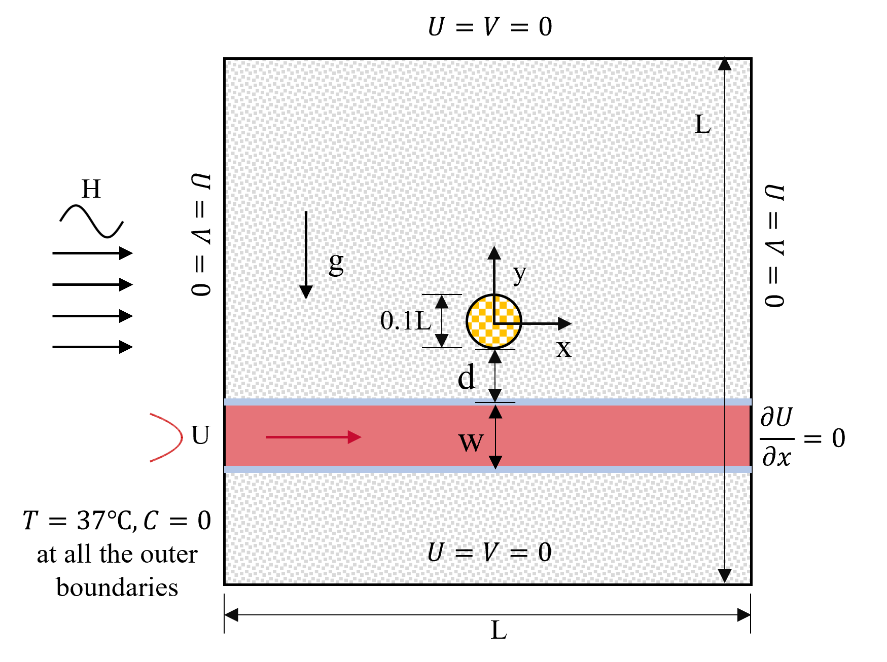
Figure 1: Schematic of magnetic hyperthermia in this study. The orange region denotes the tumor, while the gray region represents the healthy tissue. Pink channel denotes the blood vessel, and the blue lines are the vessel walls.

The schematic of this problem is presented as Figure 1, where a simplified circular tumor is located at the center of the square block. The diameter of the tumor is assumed 10 mm, which is one-tenth of the length of the whole block. Both tumor and healthy tissue are treated as porous media but with different permeability. A straight blood vessel traverses the healthy tissue at the place near the tumor with the parabolic velocity profile at the inlet and Neumann boundary at the outlet. Apart from them, other outer boundaries are stationary. The vessel walls are considered moving when involving the fluid-structure interaction effect, otherwise, they are fixed. Constant zero volume fraction and core temperature ($37^{\circ}$C) are namely adopted for the MNP and temperature boundaries. At the beginning of treatment, MNPs are uniformly distributed with 0.01 volume fraction in the tumor region, while the velocity of fluid is stationary and temperature is $37^{\circ}$C.

2.2 Governing equation

The governing equations of this multi-physics problem is given by

$$\nabla\cdot\mathbf{u}=0$$ (1a)

$$\frac{\partial\mathbf{u}}{\partial t}+(\mathbf{u}\cdot\nabla)\Big{(}\frac{\mathbf{u}}{\phi}\Big{)}=-\frac{1}{\rho_{nf}}\nabla(\phi p)+\upsilon_{nf}\nabla^{2}\mathbf{u}+\frac{\mathbf{F}}{\rho_{nf}}$$ (1b)

$$\sigma\frac{\partial T}{\partial t}+\mathbf{u}\cdot\nabla T=\alpha_{e}\nabla^{2}T+\frac{1}{(\rho c_{p})_{nf}}\dot{m}_{b}c_{pb}(T_{b}-T)+C\frac{Q}{(\rho c_{p})_{nf}}$$ (1c)

$$\phi\frac{\partial C}{\partial t}+\mathbf{u}\cdot\nabla C=D_{e}\nabla^{2}C$$ (1d)

where $\nabla\equiv\frac{\partial}{\partial x}\bm{i}+\frac{\partial}{\partial y}\bm{j}$.

Equation 1d namely lists continuity equation, momentum equation, energy equation, and concentration equation. In this holistic simulation framework, they are solved by multiple-relaxation-time Lattice Boltzmann Method (MRT-LBM), with the D2Q9 scheme on fluid field while D2Q5 scheme on temperature and concentration fields [38]. $\mathbf{u}$, $T$ and $C$ denote the fluid velocity vector (u,v) along x and y directions, temperature and MNPs volume fraction, respectively. This set of equations are adaptable in tumor tissue, healthy tissue and the blood vessel region. $\phi$ means the porosity of tissue, and $p$ means pressure. $\rho$, $c_{p}$, $\upsilon$ are fluid density, specific heat and kinetic viscosity. Since blood is a complex mixture, blood rheology is considered in part of the cases for influence study. The Carreua-Yasuda Model is applied, and it is detailed illustrated in the following section. Coefficient $\sigma=[(\rho c_{p})_{nf}\phi+(\rho c_{p})_{s}(1-\phi)]/(\rho c_{p})_{nf}$. $k_{e}=k_{nf}\phi+k_{s}(1-\phi)$ [39, 40] is the effective thermal conductivity of porous media, and effective thermal diffusivity is defined as $\alpha_{e}=k_{e}/(\rho c_{p})_{nf}$. $D_{e}=\phi D$ [40] is the effective concentration diffusivity of MNPs in porous media, and $D$ is the concentration diffusivity in pure fluid. Specifically, subscript “$nf$” denotes properties of nanofluid or modified tissue that is a mixture combining the tissue and the injected MNPs, while “$b$” denotes properties of blood, and “$s$” denotes property of tissue structure.

$\mathbf{F}$ in the last term of momentum equation (see Equation 1b) is the total external body force, including the resistance force from porous media, gravity force caused by temperature and concentration gradient, Lorentz force induced by AMF, and the body force of the immersed boundary, as [38]

$$\mathbf{F}=\frac{1}{\rho_{nf}}(-\frac{\varphi\mu_{nf}}{K}\mathbf{u}-\frac{\varphi\rho_{nf}F_{\varphi}}{\sqrt{K}}|\mathbf{u}|\mathbf{u}+\varphi\mathbf{G}+\varphi\mathbf{F_{M}}+\varphi\mathbf{F_{b}})$$ (2)

where the resistance force in porous media comes from the representative elementary volume (REV) scale method [41, 38]. $F_{\phi}$ in Equation 1d denotes the Forchheimer coefficient of porous media while $K$ denotes the permeability. $F_{\phi}$ is only determined by the porosity $\phi$ as $F_{\phi}=1.75/\sqrt{150\phi^{3}}$, but $K$ is determined by the combination of $\phi$ and mean pore diameter $d_{p}$ as $K=(\phi^{3}d_{p}^{2})/[150(1-\phi)^{2}]$. Due to the physical difference between tumor and healthy tissue, the values of permeability are not the same in their regions, and they can be separated by the subscription as $K_{tum}$ and $K_{tis}$. $|\mathbf{u}|=\sqrt{u^{2}+v^{2}}$ is the amplitude of velocity.

With the assumption of Boussinesq approximation, buoyancy force $\mathbf{G}$ is given by [42]

$$\mathbf{G}=g[(\rho\beta_{T})_{nf}(T-T_{c})+(\rho\beta_{C})_{nf}(C-C_{c})]\mathbf{j}$$ (3)

where $g$ is the acceleration of gravity. $(\rho\beta_{T})_{nf}$ and $(\rho\beta_{C})_{nf}$ are the thermal and concentration expansion of nanofluid respectively. $T_{c}$ and $C_{c}$ are namely the reference the temperature and concentration. In this study, $T_{c}$ equals to the core temperature of human body $37^{\circ}$C, and $C_{c}$ is zero volume fraction. $\mathbf{j}$ is the unit vector on y direction.

$\mathbf{F_{M}}$ is the Lorentz force that induced by a horizontal high frequency alternating magnetic field, which is converted into a steady model as in our previous work.

$$\mathbf{F_{M}}=-\frac{1}{2}\sigma_{nf}B_{0}^{2}v\mathbf{j}$$ (4)

where $\sigma_{nf}$ is the electrical conductivity of nanofluid, and $B_{0}$ is magnetic induction amplitude, which is proportional to the magnetic field intensity amplitude $H_{0}$ as $B_{0}=\mu_{0}H_{0}$, and $\mu_{0}$ is magnetic permeability of vacuum.

$\mathbf{F}_{b}$ is the boundary force from the immersed boundary method, which is illustrated in detail in B.

In energy equation (see Equation 1c), the heat sink caused by blood perfusion $\dot{m}_{b}c_{pb}(T_{b}-T)$ and the heat source induced by the MNP exposed in alternating magnetic field $CQ$ are considered. $T_{b}=37^{\circ}$C is the temperature of the blood and $\dot{m}_{b}$ is the density flow rate of temperature-dependent perfusing blood. According to Lang [43], $\dot{m}_{b}$ depends on local temperature $T$ as

In healthy tissue:

$$\dot{m}_{b}=\begin{cases}0.45+3.55\exp[-{(T-45.0)^{2}}/{12.0}]&{T\leq 45.0^{\circ}C}\\ 4.0&{T>45.0^{\circ}C}\\ \end{cases}$$ (5)

In tumor:

$$\dot{m}_{b}=\begin{cases}0.833&{T<37.0^{\circ}C}\\ 0.8333-(T-37.0)^{4.8}/{5438.0}&{37.0<T\leq 42.0^{\circ}C}\\ 0.416&{T>42.0^{\circ}C}\end{cases}$$ (6)

$Q$ is defined by the Rosensweig’s model [10] as

$$Q=\pi\mu_{0}\chi_{0}H^{2}_{0}f\frac{2\pi f\tau_{R}}{1+(2\pi f\tau_{R})^{2}}.$$ (7)

$H_{0}$ and $f$ are amplitude and frequency for external alternating magnetic field. $\chi_{0}$ denotes equilibrium susceptibility and $\tau_{R}$ denotes the effective relaxation time, which is determined by both Neel and Brownian relaxation time [8].

The following parameters are used to nondimensionalize the governing equation,

$$\begin{split}X=\frac{x}{L},\;Y=\frac{y}{L},\;U=\frac{u}{U_{0}},\;V=\frac{v}{U_{0}},\;\tau=\frac{tU_{0}}{L},\\ P=\frac{p}{\rho_{f}U_{0}^{2}},\;\theta=\frac{T-T_{c}}{T_{h}-T_{c}},\;\varphi=\frac{C-C_{c}}{C_{h}-C_{c}}\end{split}$$ (8)

Then the dimensionless governing equation is given by

$$\nabla\cdot\mathbf{U}=0$$ (9a)

$$\begin{split}&\frac{\partial\mathbf{U}}{\partial\tau}+(\mathbf{U}\cdot\nabla^{*})\Big{(}\frac{\mathbf{U}}{\phi}\Big{)}\\ &=-\frac{\rho_{f}}{\rho_{nf}}\nabla^{*}(\phi P)+\frac{1}{Re}\frac{\upsilon_{nf}}{\upsilon_{f}}\nabla^{*2}\mathbf{U}-\phi\frac{\upsilon_{nf}}{\upsilon_{f}}\frac{1}{Re\cdot Da}\mathbf{U}-\phi\frac{F_{\phi}}{\sqrt{Da}}\sqrt{|\mathbf{U}|}\mathbf{U}\\ &+[\phi\frac{(\rho\beta)_{nf}}{(\rho\beta)_{f}}\frac{\rho_{f}}{\rho_{nf}}Ra\frac{Re^{2}}{Pr}(\theta+N\varphi)-\phi\frac{\sigma_{nf}}{\sigma_{n}}\frac{\rho_{f}}{\rho_{nf}}Ha^{2}Pr\mathbf{U}]\mathbf{j}\end{split}$$ (9b)

$$\sigma\frac{\partial\theta}{\partial\tau}+\mathbf{U}\cdot\nabla^{*}\theta=\frac{\alpha_{e}}{\alpha_{f}}\nabla^{*2}\theta-\frac{(\rho c_{p})_{f}}{(\rho c_{p})_{nf}}\frac{Pe}{Re\cdot Pr}\theta+\varphi\frac{(\rho c_{p})_{f}}{(\rho c_{p})_{nf}}\frac{Q_{0}}{Re\cdot Pr}$$ (9c)

$$\phi\frac{\partial\varphi}{\partial\tau}+\mathbf{U}\cdot\nabla^{*}\varphi=\frac{\phi}{Le}\nabla^{*2}\varphi$$ (9d)

From the above dimensionless governing equations, this problem is characterized by the following dimensionless parameters:

$$Re=\frac{U_{0}L}{\upsilon_{f}}$$ (10a)

$$Pr=\frac{\upsilon_{f}}{\alpha_{f}}$$ (10b)

$$Le=\frac{\alpha_{f}}{D}$$ (10c)

$$Da=\frac{K}{L^{2}}$$ (10d)

$$Ra=\frac{\beta_{T}g(T_{h}-T_{c})L^{3}}{\upsilon_{f}\alpha_{f}}$$ (10e)

$$N=\frac{\beta_{C}(C_{h}-C_{c})}{\beta_{T}(T_{h}-Tc)}$$ (10f)

$$Ha^{2}=\frac{\sigma_{n}\mu_{0}^{2}H_{0}^{2}L^{2}}{\rho_{f}\upsilon_{f}}$$ (10g)

$$Pe=\frac{\dot{m}_{b}c_{pb}L^{2}}{(\rho c_{p})_{f}\alpha_{f}}$$ (10h)

$$Q_{0}=\frac{QL^{2}(C_{h}-C_{l})}{(\rho c_{p})_{f}\alpha_{f}(T_{h}-T_{c})}$$ (10i)

in which, the parameters $Re$ $Pr$, $Le$, $Da$, $N$, $Ha$, $Pe$ and $Q_{0}$ are Reynolds number, Prandtl number, Lewis number, Darcy number, buoyancy ratio, Hartmann number, Peclet number and heat source number.

Additionally, for the reason of different permeability in tumor and tissue, the Darcy ratio is

$$R_{Da}=\frac{Da_{tum}}{Da_{tis}}=\frac{K_{tum}}{K_{tis}}$$ (11)

The effective properties of tissue fluid should be modified by considering the influence of interspersed MNPs, and they are computed from [44, 45]

$$\rho_{nf}=C\rho_{n}+(1-C)\rho_{f}$$ (12a)

$$\upsilon_{nf}=\frac{\mu_{f}}{\rho_{nf}(1-C)^{2.5}}$$ (12b)

$$(\rho c_{p})_{nf}=C(\rho c_{p})_{n}+(1-C)(\rho c_{p})_{f}$$ (12c)

$$(\rho\beta_{T})_{nf}=C(\rho\beta_{T})_{n}+(1-C)(\rho\beta_{T})_{f}$$ (12d)

$$k_{nf}=k_{f}\frac{k_{n}+2k_{f}-2C(k_{f}-k_{n})}{k_{n}+2k_{f}+C(k_{f}-k_{n})}$$ (12e)

$$\sigma_{Enf}=\sigma_{Ef}\frac{\sigma_{En}+2\sigma_{Ef}-2C(\sigma_{Ef}-\sigma_{En})}{\sigma_{En}+2\sigma_{Ef}+C(\sigma_{Ef}-\sigma_{En})}$$ (12f)

where the subscript “$f$” means pure fluid and “$n$” means nanoparticles in Equation 9d and Equation 12f. In this study, pure fluid represents the interstitial tissue fluid and blood flow, in which distributes the MNP $Fe_{3}O_{4}$. The kinetic and thermal proprieties of them are listed as Table 1 [46, 45, 30].

Table 1: Properties of nanofluid

Properties for tissue	Value	Properties for MNPs	Value
$\rho_{f}(kg/m^{3})$	1052	$\rho_{n}(kg/m^{3})$	5200
$k_{f}(W/mK)$	0.5	$k_{n}(W/mK)$	6
$c_{pf}(J/kgK)$	3800	$c_{pn}(J/kgK)$	670
$\beta_{Tf}(1/K)$	$2.1\times 10^{-4}$	$\beta_{Tn}(1/K)$	$1.3\times 10^{-5}$
$\sigma_{Ef}(\Omega^{-1}\cdot m^{-1})$	0.7	$\sigma_{En}(\Omega^{-1}\cdot m^{-1})$	$2.5\times 10^{4}$
$\mu_{f}(Pa\cdot s)$	$6.92\times 10^{-4}$	-	-

2.3 Thermal dose

The cumulative-equivalent-minutes-at-$43^{\circ}C$ (CEM43) model is widely accepted in thermal dose evaluating, by converting the treatment to an equivalent time on $43^{\circ}C$, as

$$CEM43=\sum_{i=1}^{l}{C_{EM}}^{43-T_{i}}\delta t$$ (13)

where $T_{i}$ is the averaged temperature in ${}^{\circ}C$ at the $i$th time steps, $\delta t$ represents the time interval, and $l$ denotes the total number of time steps. ${C_{EM}}$ equals to 0.5 when $T_{i}>43^{\circ}C$ and 0.25 otherwise [37]. As CEM43 achieves 60 minutes, cells are regarded totally destroyed [12, 34]. Upon this hypothesis, an ablated area ratio in tumor or surrounding healthy tissue is defined for therapeutic efficacy, i.e.

$$R_{CEM43}=\frac{S_{CEM43\geq 60min}}{S_{tum}}$$ (14)

The optimal result of $R_{CEM43}$ in tumor and healthy tissue are 1 and 0, respectively, in accordance with the expected hyperthermia treatment efficacy - totally killing the tumor cells but without destroying the healthy tissue,

3 Results and discussion

3.1 Baseline case

The baseline case uses the properties from practical problems. Dimensionless parameters that computing from the physical case [22, 46, 28, 47, 48] are listed as Table 2.

Table 2: Dimensionless parameters on baseline case

Parameters	Value
$Re$	$100$
$Ra_{T}$	$2.05\times 10^{8}$
$Pr$	$5.26$
$Le$	$125.08$
$N$	$-18.78$
$Ha$	$4.27$3
$Q$	$572.73$
$Da_{tis}$	$2.00\times 10^{-11}$
$R_{Da}$	$4.84$
$\phi$	$0.26$

3.2 Effect of blood vessel

To explore the effect of the nearby blood vessel on the magnetic hyperthermia treatment efficacy, a vessel with $w=5mm$ and $d=0mm$ is employed for discussion. Figure 2 illustrates the effect of a nearby blood vessel on the MNP concentration and temperature. For easy comparison, two instants are taken into consideration, namely $t=30$ min and $t=60$ min. For the MNPs distribution, they diffuse obviously with time, and the flow in the blood vessel washes away the MNPs in it. Although vanishing in the vessel part, the shape of MNP distribution in healthy tissue and tumor keeps unchanged except for that near the vessel wall. For the temperature profile, the effect seems much more considerable. The maximum temperature drops with time as MNP diffusion. As Figure 2 (e), the most value of temperature exceeds $46^{\circ}C$, but there is only $44^{\circ}C\sim 45^{\circ}C$ in Figure 2 (f), which is a similar difference between Figure 2 (g) and (h). This means the blood vessel has a significant cooling effect on the temperature distribution of the nearby region, the came consequence as discussed in [29].

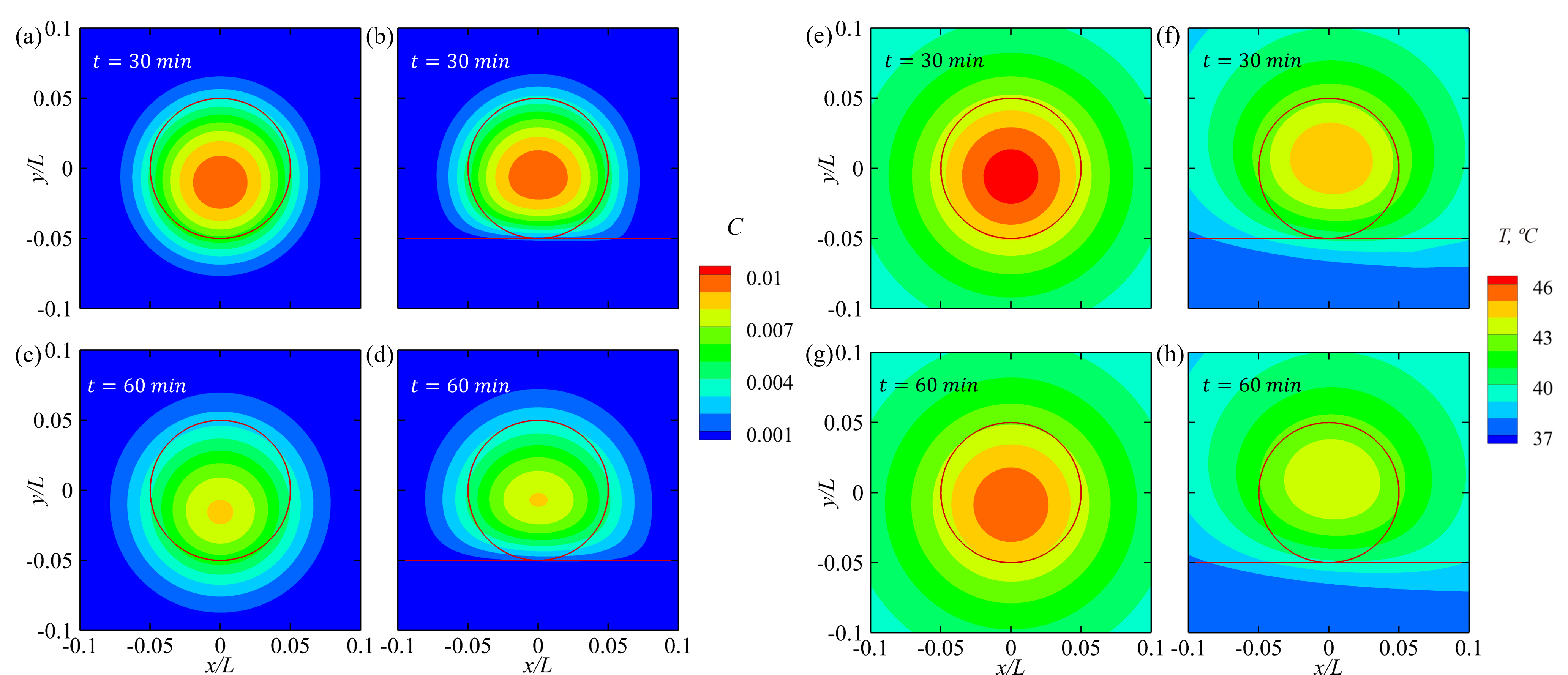
Figure 2: Effect of a nearby blood vessel on the MNP concentration and temperature at treatment time $t=30$ min and $t=60$ min. (a) $\sim$ (d) denote the MNP distribution, for no vessel case at (a) $t=30$ min and (c) $t=60$ min, and for vessel case at (b) $t=30$ min and (d) $t=60$ min. (e) $\sim$ (h) present the temperature profile for no vessel case at (a) $t=30$ min and (c) $t=60$ min, and for vessel case at (b) $t=30$ min and (d) $t=60$ min.

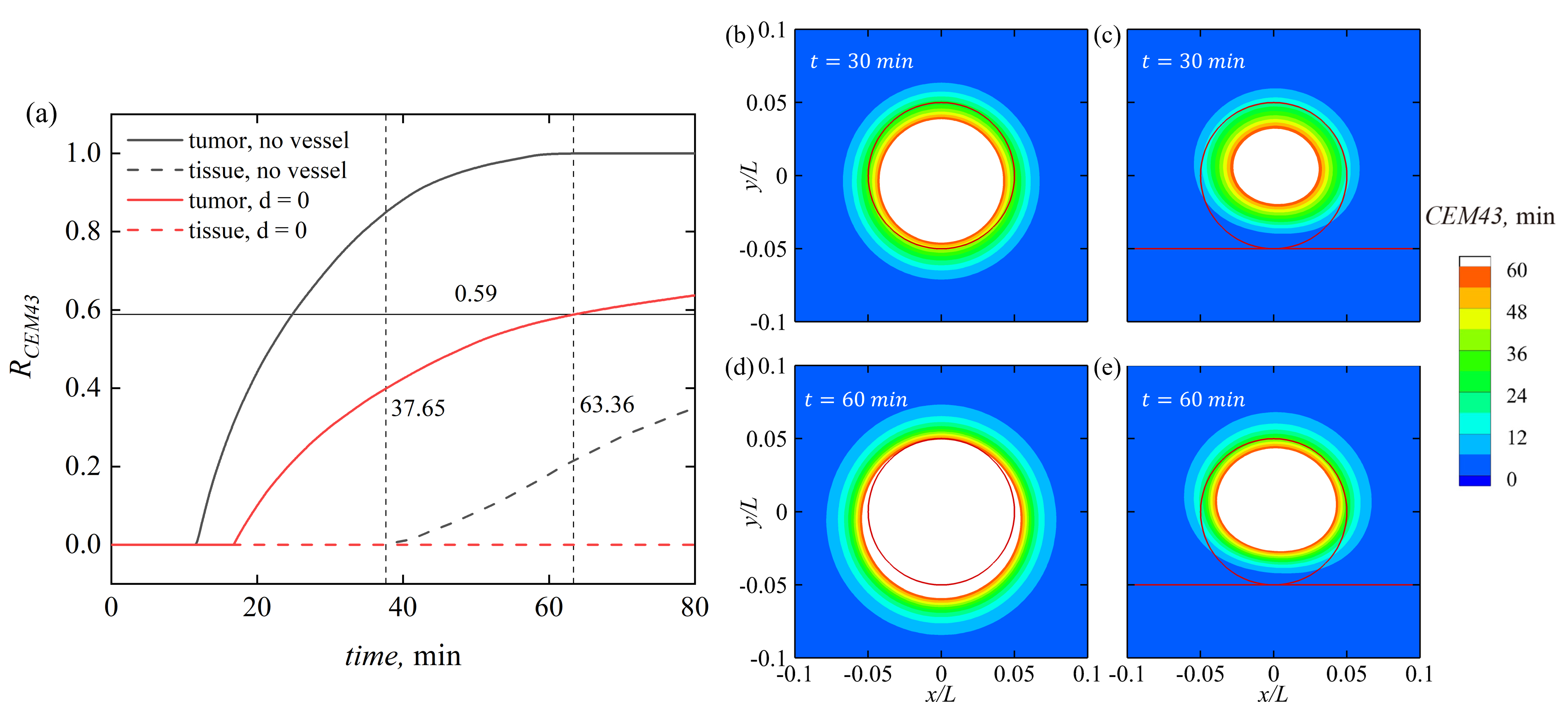
Figure 3: Effect of a nearby blood vessel on the thermal dose CEM43. (a) denotes $R_{CEM43}$ evolution in tumor and healthy tissue of cases with the nearby blood vessel or not. (b) $\sim$ (e) the CEM43 distribution, for no vessel case at (b) $t=30$ min and (d) $t=60$ min, and for vessel case at (c) $t=30$ min and (e) $t=60$ min. White regions in (b) $\sim$ (e) denote the ablation part.

Figure 3 (a) demonstrates the evolution of $R_{CEM43}$, where solid curves represent the situations of the tumor while the dashed curves are for healthy tissue. It is evident that $R_{CEM43}$ of no vessel case elevates much faster than that of vessel case. The tumor has been totally destroyed for no vessel case at $t=63.36$ min, but at the same time there are only 59% tumor cells ablated for vessel case, nearly half of no vessel case. Additionally, for no vessel case, healthy tissue begins to be killed at treatment time $t=37.65$ min, but for no vessel case, still no cell is injured when the heat process lasts for 80 min. Therefore, the cooling effect of the blood vessel significantly diminishes the heating process and prolongs the treatment time. This is also reflected in the distribution of CEM43. For each instance, the ablation part is noticeably larger for no vessel case, and the whole ablation area are namely 2.36 and 2.06 times that of the vessel case. These data can be also discovered in the Table 3. The table reveals the effect of the blood vessel on parameters in detail. As table listed, the location of $T_{max}$ marginally moves upwards and rightwards, while the $C_{max}$ moves upwards.

Table 3: Effect of a blood vessel on the parameters of magnetic hyperthermia treatment

$t$, min	30		60
Condition	No vessel	With vessel	No vessel	With vessel
$T_{max}$	46.49	44.93	45.74	43.93
Location of $T_{max}$	(0.4,0.495)	(0.5025,0.505)	(0.5,0.495)	(0.5025,0.5075)
$C_{max}\cdot 10^{-3}$	9.64	9.70	8.17	8.07
Location of $C_{max}$	(0.5,0.49)	(0.5,0.495)	(0.5,0.485)	(0.5,0.4925)
$R_{CEM43}$ in tum.	0.711	0.301	0.998	0.573
$R_{CEM43}$ in healthy tis.	0	0	0.18	0

3.3 Effect of gravity

As discussed in our previous work, gravity influences treatment efficacy when a tumor is surrounded by healthy tissue. Therefore, this chapter also investigates the effect of gravity when the tumor is near a blood vessel. The cases without gravity are included for comparison with three different distances to the tumor boundary, namely $d=0$ mm, $d=2$ mm, and $d=4$ mm.

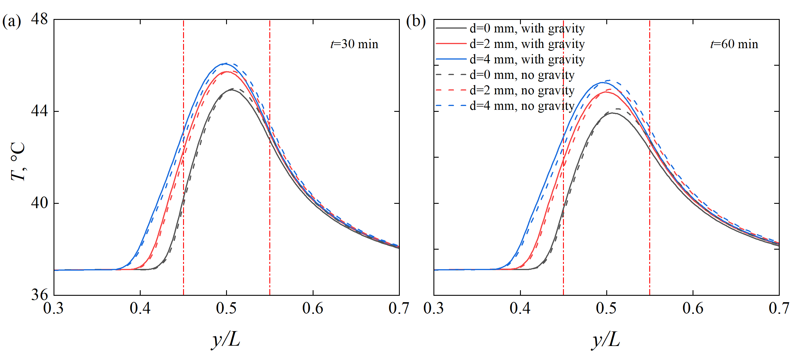
Figure 4: Effect of gravity on temperature profile along $y/L=0.5$ at treatment time (a) $t=30$ min and (b) $t=60$ min. Vertical red dash-dot lines denote the tumor boundary.

Figure 4 presents the temperature distribution at the vertical midline. It is not surprising to discover a downward tendency of the temperature profile and a little reduction on the maximum temperature with gravity, but this change is much weak. Although the difference enlarges with time, it is still very limited from about $0.05^{\circ}C$ to about $0.1^{\circ}C$.

Table 4: Effect of gravity on $R_{CEM43}$ at treatment time $t=60$ min

$d$, mm	Parameter	No gravity	Gravity
4	$R_{CEM43}$ in tumor, %	95.62	97.77
	$R_{CEM43}$ in healthy tissue, %	4.4	0.87
2	$R_{CEM43}$ in tumor, %	85.52	85.82
	$R_{CEM43}$ in healthy tissue, %	1.19	0.00
0	$R_{CEM43}$ in tumor, %	59.24	57.32
	$R_{CEM43}$ in healthy tissue, %	0.00	0.00

Table 4 lists the value of $R_{CEM43}$ at $t=60$ min. Generally, the existence of gravity elevates the treatment efficacy to some extent, which performs best in the case $d=4$ mm. As the results unveil, gravity leads to more ablation on the tumor but less on healthy tissue when distance equals to 4 mm, as already 97.77% and only 0.87%, respectively. This outcome gets pretty close to the theoretically best results, 100% in tumor and 0% in healthy tissue. In the case of $d=2$ mm, although $R_{CEM43}$ in tumor shows equality, there is 1.19% injury in healthy tissue without gravity but no ablation with gravity. They are also reflected in Figure 5. It is not difficult to understand that gravity effect moves downwards the ablation region, which cooperates with the cooling effect of the blood vessel and performs best at the distance $d=4$ mm as Figure 5 (c). In addition, Figure 5 and Table 4 also indicates the essential influence from the distance from the upper blood vessel wall to the tumor boundary. Therefore, the investigation of distance $d$ is also discussed.

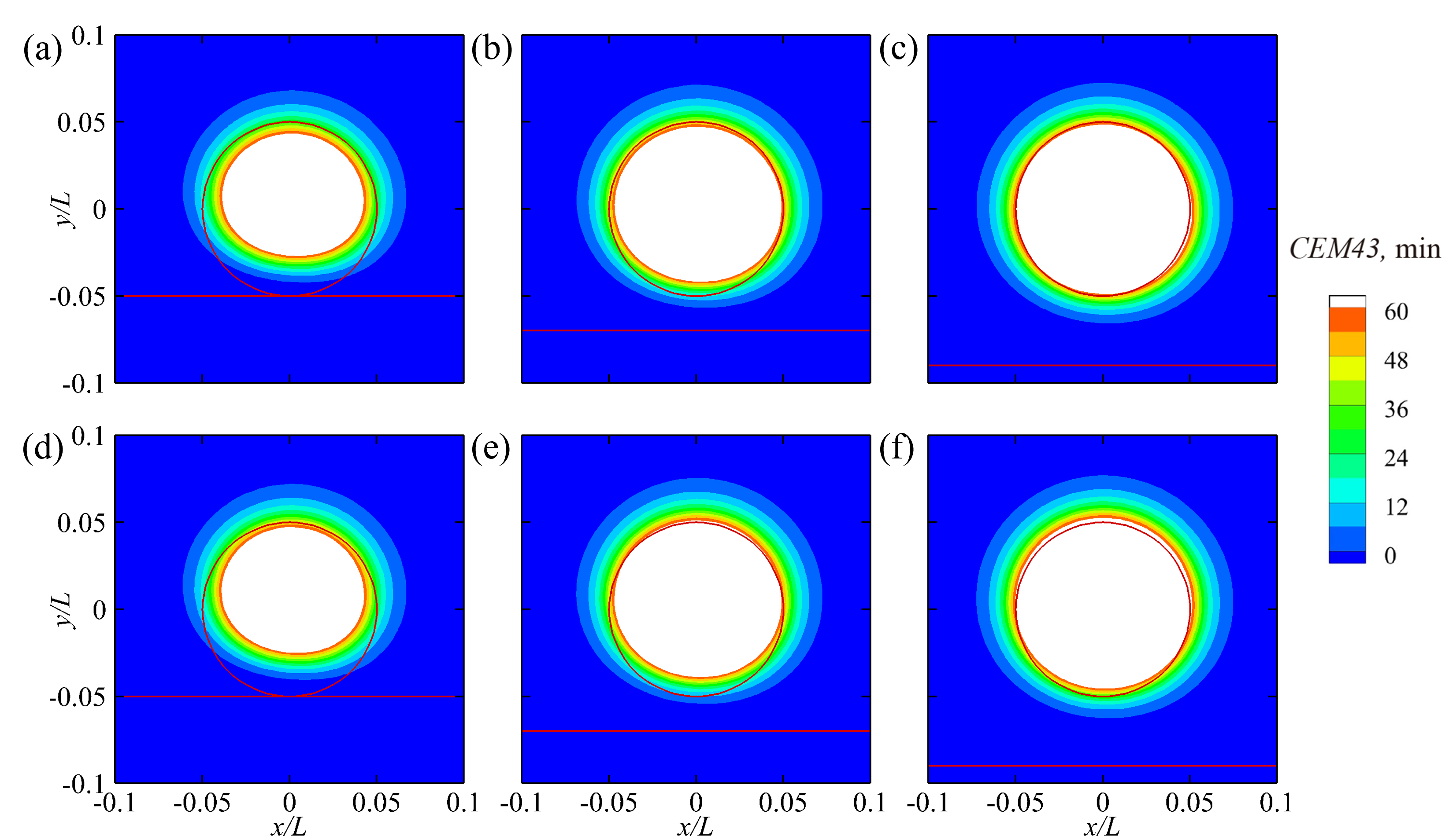
Figure 5: Effect of gravity on $CEM43$ distribution. (a) $\sim$ (c) denote the situations affected by gravity with the distance to tumor boundary (a)$d=0$ mm, (b)$d=2$ mm, and (c)$d=4$ mm. (d) $\sim$ (f) denote the situation without gravity. The red circle means the tumor boundary, and the horizontal red lines point the location of the blood vessel. White color is the ablation part.

3.4 Effect of distance

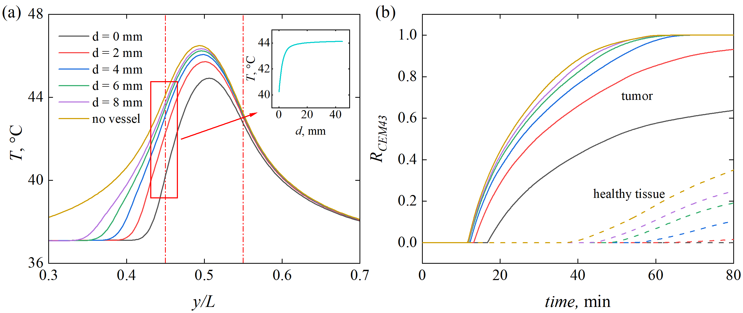
Figure 6: Effect of distance between blood vessel upper boundary to the tumor boundary $d$ at treatment time $t=30$ min. (a)The temperature profile at the midline of $x/L=0.5$, and (b) $R_{CEM43}$ evolution in tumor and healthy tissue, with the variation of distance $d$. Vertical red dash-dot lines denote the boundary of the tumor.

To explore the important influence of distance from the upper boundary of blood vessel to the nearest tumor boundary, six cases are employed with the variation of distance $d=$ 0 mm, 2 mm, 4 mm, 6 mm, 8 mm, and $\infty$ (no vessel case). The data reveal that when distance $d$ gradually rises from 0 mm, the temperature profile is continuously approaching to the case without the blood vessel as Figure 6 (a). This change is remarkable at the lower tumor boundary, where the temperature increases from $40.22^{\circ}C$ for $d=0$ mm to $43.75^{\circ}C$ for $d=8$ mm. Noticeably, the temperature at the lower tumor boundary for the no vessel case is $44.12^{\circ}C$, so the case with distance $d=8$ mm shows 0.8% diffidence to that value. Not surprisingly, treatment processing slows down a lot for distance $d=0$ mm, in which only 63.77% tumor cells are destroyed at treatment $t=80$ min. When distance $d$ augments to 2 mm, the situation gets better. There has been 93.16% injury and 1.35% at treatment time $t=80$ min. The cases with distance $d=$4, 6, and 8 are closer to the no vessel case, and especially, the time for totally killing the tumor cells with the distance $d=8$ mm is 65.66 min, 3.64% longer than that of no vessel case.

3.5 Effect of the width of blood vessel

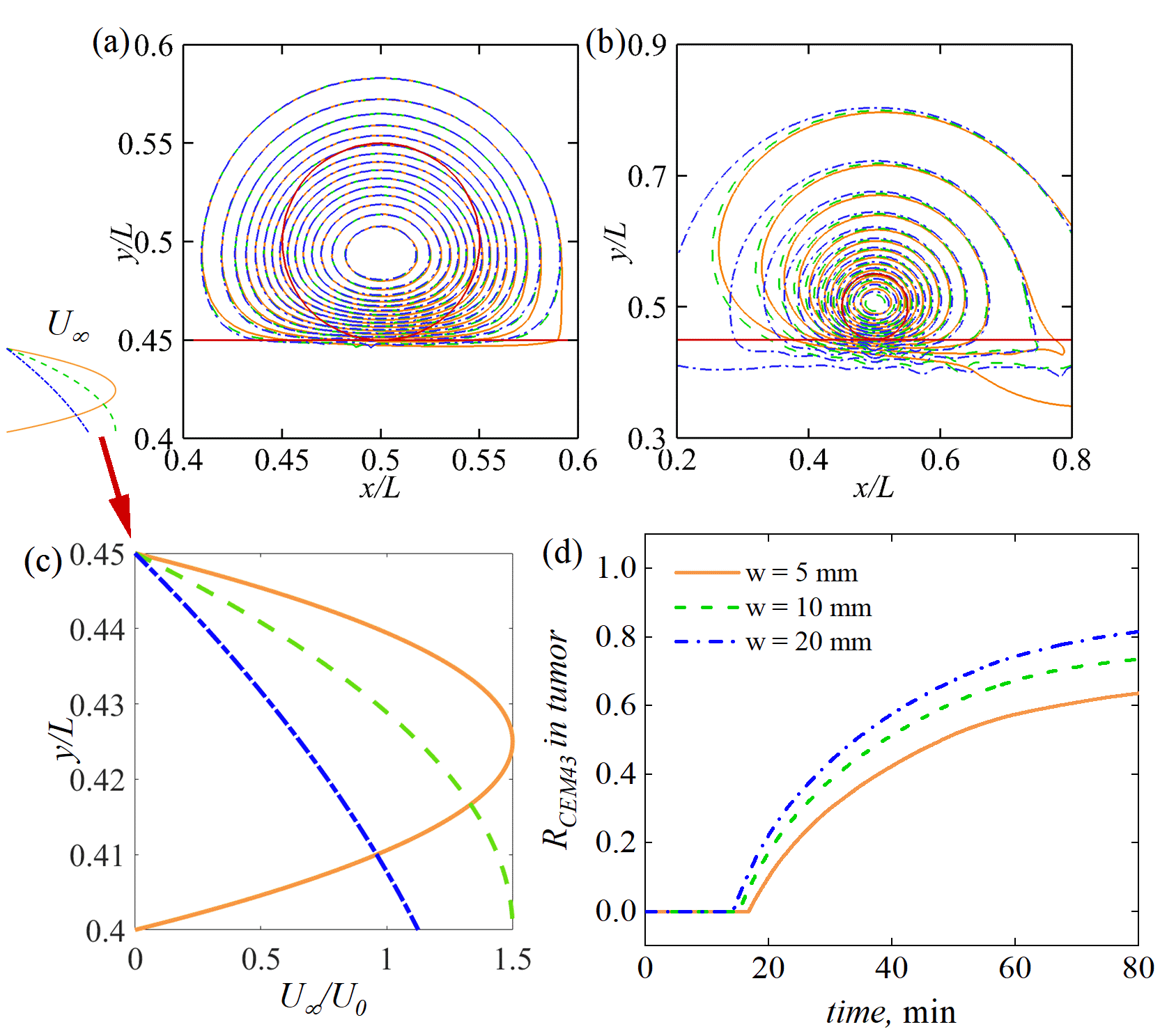
Figure 7: Effect of the width $w$ of the blood vessel on (a) MNP concentration distribution at $t=60$ min, (b) temperature distribution at $t=60$ min, and (d) the evolution of $R_{CEM43}$ in tumor. (c) presents the velocity profile at the vessel inlet. The red circle is the tumor boundary, while the horizontal red line means the upper boundary of the blood vessel.

The same mean velocity at the blood vessel inlet but the different width vessel is imposed, which leads to a changeable velocity gradient near the upper boundary of the vessel. In this part, the distance from the vessel to the tumor is still $d=0$ mm. Then vessel flow ranges in $y/L=$ [0.4,0.45] for $d=5$ mm, in $y/L=$ [0.35,0.45] for $d=10$ mm, and $y/L=$ [0.25,0.45] for $d=20$ mm. As illustrated in Figure 7 (c), there shows a width of 5 mm from the upper blood vessel downwards. Obviously, the thinner the blood vessel, the larger the velocity gradient near the upper vessel wall (adjacent to the tumor). In Figure 7 (a), almost all the contour lines on the MNP concentrations are overlapped except for a little part much near the vessel. This is consistent with the analysis in Section 3.2. However, the isotherms obtain a large divergence among the three cases not only significantly performing near the blood vessel but also the upstreaming region of the tumor (see Figure 7 (b)). As the width of the vessel extends, the area of the same isotherm expands, and the maximum temperature elevates as Table 5. This change surely results in the difference to tumor treatment efficacy. Regarding the Figure 7 (d), a considerable benefit is added when the width of the blood vessel converts from 5 mm to 20 mm, which has been quantified in Table 5.

Table 5: Effect of blood vessel width on maximum temperature and $R_{CEM43}$ in tumor at treatment time $t=60$ min.

$w$, mm	5	10	20
$T_{max}$, ${}^{\circ}C$	43.93	44.19	44.39
$R_{CEM43}$ in tumor, %	57.32	67.27	74.76

3.6 Effect of vessel direction

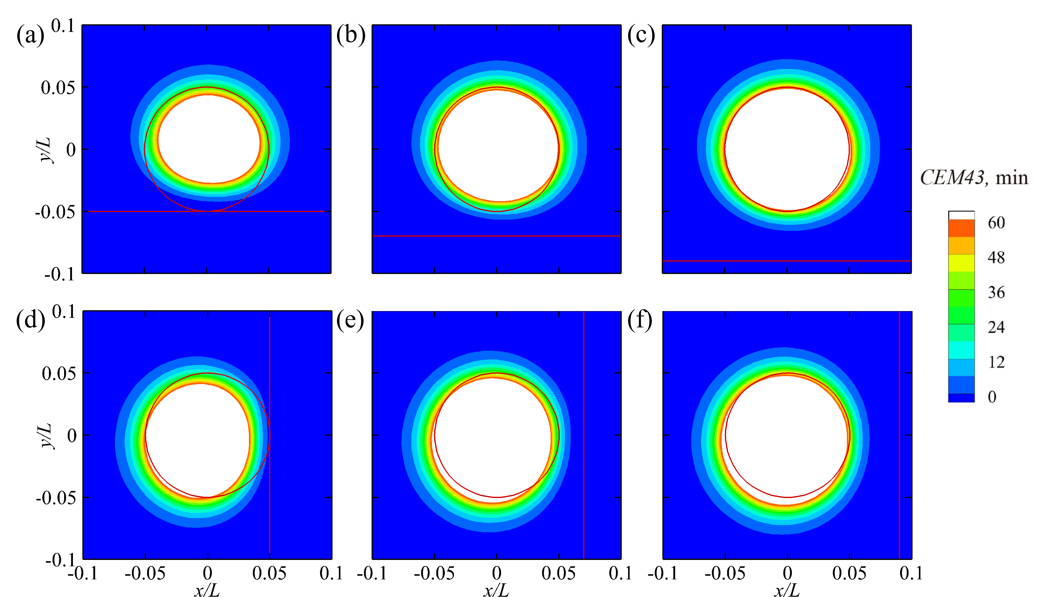
Figure 8: Effect of vessel direction of blood vessel on the CEM43 distribution at treatment time $t=60$ min. Horizontal blood vessel with distance (a) $d=0$ mm, (b) $d=2$ mm, and (c) $d=4$ mm. Downwards vertical blood vessel with distance (a) $d=0$ mm, (b) $d=2$ mm, and (c) $d=4$ mm. The red circle means the tumor boundary, while the red horizontal/vertical line denotes the blood vessel boundary towards the tumor side.

Figure 8 displays the effect of blood vessel direction on treatment efficacy. As discussed in Section 3.3, the collaboration of downward gravity and the proper cooling effect of the blood vessel from the lower part makes the horizontal vessel with $d=4$ mm the best performance among the horizontal cases. However, the downward vertical vessel cools down the temperature from the right part, which cannot cancel the side effects of gravity, causing an easy-ablation region to the southwest of the tumor and a hard-ablation region in the opposite tumor domain. $R_{CEM43}$ at $t=60$ min treatment time can be found in the Table 6, a similar consequence can be drawn with which.

Table 6: Effect of blood vessel direction on $R_{CEM43}$, %

$d$, mm	Position	Horizontal	Vertical
4	Tumor	97.77	96.18
	Healthy tissue	0.87	8.75
2	Tumor	85.52	90.37
	Healthy tissue	0.00	5.49
0	Tumor	57.32	75.42
	Healthy tissue	0.00	1.51

3.7 Effect of moving vessel boundary

In this part, the moving boundary of blood vessel walls is involved to explore the influence of which. The width of blood vessel is $w=10$ mm, and the variation of vessel width is $\Delta w=0.04w$. The results of traditional bounce-back, fixed IB, sine wave IB (wavelength $\lambda=L$, frequency $f=1$ Hz, and phase difference $\Delta\phi=\pi/4$ ), and pulsation wave IB (referred to [33]) are listed in Table 7 for comparison. Results indicate that, for the simulated case, there exists only a little variation on $R_{CEM43}$ in tumor and healthy tissue for four different vessel boundaries, even the moving IB boundaries, which means moving boundary does not bring a significant influence on magnetic hyperthermia treatment. In addition, we compare the isotherms of fixed IB and sine wave IB as Figure 9. Figures confirm there is almost no impact on the treatment efficacy.

Table 7: Effect of moving blood vessel wall on $R_{CEM43}$ in tumor and healthy tissue at treatment time $t=60$ min.

$d$, mm	Condition	Position	Fixed BB	Fixed IB	Sine IB	Pulsation IB
2	No gravity	Tumor	88.78	89.50	89.58	89.82
		Healthy tissue	1.83	2.23	1.91	1.59
	Gravity	Tumor	93.48	93.72	93.72	92.84
		Healthy tissue	0.32	0.24	0.16	0.08
0	No gravity	Tumor	67.28	67.13	68.81	-
		Healthy tissue	0.00	0.00	0.00	-

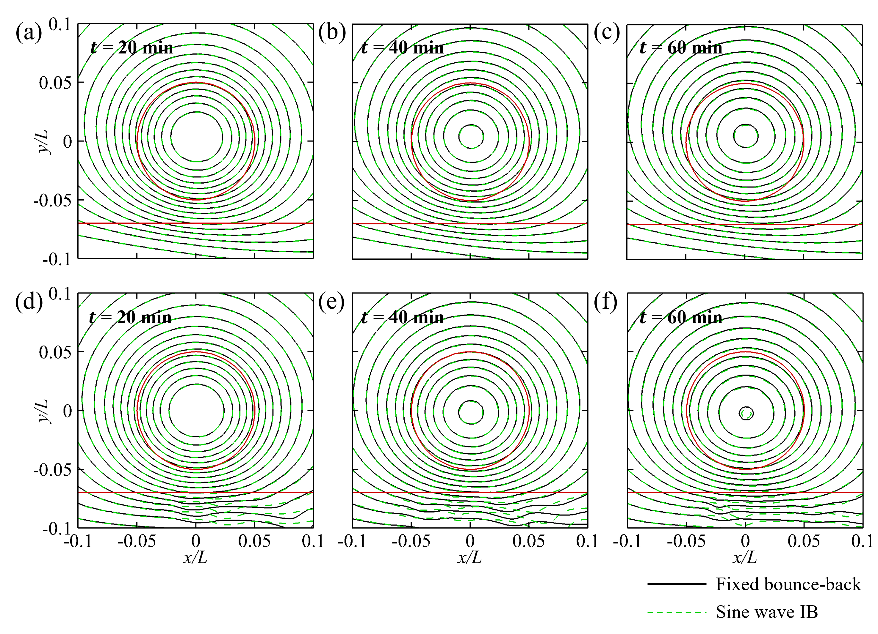
Figure 9: Effect of moving vessel on the isotherms. (a) $\sim$ (c) denote the isotherms with no gravity effect. (d) $\sim$ denote the isotherms with the gravity effect.

3.8 Effect of blood rheology

Blood is a shear-rate-dependent non-Newtonian fluid. In this part, Carreua-Yasuda Model is applied to study the influence of blood rheology (see C for details). Values of the parameter in Carreua-Yasuda Model are $\eta_{0}=0.056$ Pa$\cdot$s, $\eta_{\infty}=0.00345$ Pa$\cdot$s, $\lambda=3.313$ s, $n=0.22$, $a=1.25$ [32]. The comparison with Newtonian on $R_{CEM43}$ is listed in the table 8. Since blood is regarded as a shear-thinning viscous flow, the velocity gradient near the vessel wall behaves a little larger than that of non-Newtonian. Not surprisingly, the degree of ablation in tumor and healthy tissue, therefore, is a bit more moderate. This is consistent with the effect of the vessel width.

Table 8: Effect of blood rheology on $R_{CEM43}$ (Unit: %) at treatment time $t=60$ min

$d$, mm	Position	Newtonian	Carreua-Yasuda Model
2	Tumor	89.50	89.10
	Healthy tissue	2.23	1.83
0	Tumor	69.13	67.06
	Healthy tissue	0.00	0.00

4 Conclusion

This study developed a holistic simulation framework for magnetic hyperthermia cancer treatment and investigated the situations when the tumor is near a blood vessel. Simulation involves the blood and interstitial tissue flow, MNP distribution, temperature profile, and the behaviors of nanofluids. The treatment efficacy is evaluated with the thermal dose CEM43 model. We investigate the influence of the nearby blood vessel, the distance from the vessel to the tumor, the width of the vessel, the direction of the vessel, the moving vessel wall, and the blood rheology.

According to the results, the nearby vessel has a significant cooling effect on the treatment. A vessel next to the tumor can reduce the ablation areas to less than half. Gravity creates a downward tendency of temperature profile and a little reduction in the maximum temperature, but these changes seem much more limited compared with the influence of the distance. Although narrow, the downward influence combines the upward cooling effect from the vessel, resulting in the best performance in treatment at distance $d=4$ mm. A smaller distance from the tumor to the vessel cools down the temperature a lot, therefore considerably prolonging the treatment procedure. However, the effect on temperature almost vanishes as distance expends to 8 mm. Width the same mean velocity, divergence widths of the blood vessel cause the different velocity gradient near the vessel wall. The thinner the blood vessel, the lower the temperature profile, and the slower the tumor ablation pace. Not fortunate as the horizontal vessel, the downward vertical vessel cools the temperature from the right part, which cannot reduce the gravity effect on treatment, so the performance is inferior to the horizontal blood vessel. Blood rheology leads to a little larger gradient near the vessel wall, then resulting in a bit more moderate ablation process. Moving vessel boundaries exert the bare impact on the treatment efficacy.

Appendix A Lattice Boltzmann method

The LBM is a relatively new CFD method for fluid flow and heat/mass transfer simulations. Unlike traditional CFD methods, which solve the conservation equations of macroscopic properties numerically, LBM models the fluid particles by distribution functions through consecutive streaming and collision processes over a number of square lattices [49, 50, 51]. Zhang [46] was probably the first to apply the LBM to solving PBHTE, successfully demonstrating the capability of LBM in simulating bioheat problems. This mesoscopic approach was then widely applied for bioheat studies [15, 52, 53]. In the present study, a D2Q9 (i.e., two-dimensional nine-discrete-velocity) MRT (i.e., multiple-relaxation-time, a collision model that is used to improve the numerical stability [54]) and a D2Q5 (i.e., two-dimensional five-discrete-velocity) MRT LBM scheme are namely applied to obtain the vector field (flow field) and scalar field (temperature field and concentration field) by solving Equation 1d [38, 42].

The discrete D2Q9 MRT-LBM equation for velocity field is written as

$$\mathbf{f}(x_{k}+\mathbf{e}\delta_{t},t_{n}+\delta_{t})-\mathbf{f}(x_{k},t_{n})=-\mathbf{M}^{-1}\mathbf{\Lambda}[\mathbf{m}-\mathbf{m}^{(eq)}]|_{(x_{k},t_{n})}+\mathbf{M}^{-1}\delta_{t}(1-\frac{\mathbf{\Lambda}}{2})\mathbf{S}$$ (15)

where $\mathbf{f}(x_{k},t_{n})$ is nine-dimensional distribution function vectors at time ${t}_{n}$ and node $x_{k}$ for fluid field. $\mathbf{m}$ and $\mathbf{m}^{(eq)}$ are moment and the corresponding equilibrium moment vector for flow field. $\mathbf{e}$ describes unit velocities along 9 discrete directions

$$e_{i}=\begin{cases}(0,0)&{i=0}\\ (\cos{[(i-1)\pi/2]},\sin{[(i-1)\pi/2]})c&{i=1\sim 4}\\ (\cos{[(2i-9)\pi/4]},\sin{[(2i-9)\pi/4]})\sqrt{2}c&{i=5\sim 8}\end{cases}$$ (16)

where $c=\delta_{x}/\delta_{t}$ is the lattice speed, which is 1 since $\delta_{x}=\delta_{t}$ in the MRT model. $\mathbf{M}$ is a $9\times 5$ orthogonal transformation matrix

$$\mathbf{M}=\begin{pmatrix}1&1&1&1&1&1&1&1&1\\ -4&-1&-1&-1&-1&2&2&2&2\\ 4&-2&-2&-2&-2&1&1&1&1\\ 0&1&0&-1&0&1&-1&-1&1\\ 0&-2&0&2&0&1&-1&-1&1\\ 0&0&1&0&-1&1&1&-1&-1\\ 0&0&-2&0&2&1&1&-1&-1\\ 0&1&-1&1&-1&0&0&0&0\\ 0&0&0&0&0&1&-1&1&-1\end{pmatrix}$$ (17)

$\mathbf{\Lambda}$ is the nine-dimensional diagonal relaxation matrix

$$\mathbf{\Lambda}=\text{diag}(1,1.1,1.1,1,1.2,1,1.2,1/\tau_{\upsilon},1/\tau_{\upsilon})$$ (18)

and $\tau_{\upsilon}$ can be recovered to viscosity of nanofluid in Chapman–Enskog analysis on Equation 1d as

$$\upsilon_{nf}=\sigma c_{s}^{2}(\tau_{\upsilon}-0.5)\delta_{t}$$ (19)

$\mathbf{S}$ is the external force vector in the moment space, which is linked to the body force $F$ in governing equation 1d(b).

The discrete D2Q5 MRT-LBM equation for temperature and concentration fields are written as

$$\mathbf{g}(x_{k}+\mathbf{e}\delta_{t},t_{n}+\delta_{t})-\mathbf{g}(x_{k},t_{n})=-\mathbf{N}^{-1}\mathbf{\Theta}[\mathbf{n_{g}}-\mathbf{n_{g}}^{(eq)}]|_{(x_{k},t_{n})}+\mathbf{N}^{-1}\delta_{t}\mathbf{\Psi}$$ (20a)

$$\mathbf{h}(x_{k}+\mathbf{e}\delta_{t},t_{n}+\delta_{t})-\mathbf{h}(x_{k},t_{n})=-\mathbf{N}^{-1}\mathbf{\Upsilon}[\mathbf{n_{h}}-\mathbf{n_{h}}^{(eq)}]|_{(x_{k},t_{n})}$$ (20b)

where $\mathbf{g}(x_{k},t_{n})$ and $\mathbf{h}(x_{k},t_{n})$ are five-dimensional distribution function vectors at time ${t}_{n}$ and node $x_{k}$ for temperature and concentration respectively. $\mathbf{n}$ and $\mathbf{n}^{(eq)}$ are moment and the corresponding equilibrium moment vector, respectively, where subscribe ”g” represents temperature field and ”h” denotes concentration field. $\mathbf{e}$ describes unit velocities along 5 discrete directions

$$e_{i}=\begin{cases}(0,0)&{i=0}\\ (\cos{[(i-1)\pi/2]},\sin{[(i-1)\pi/2]})c&{i=1\sim 4}\\ \end{cases}$$ (21)

$\mathbf{N}$ is a $5\times 5$ orthogonal transformation matrix

$$\mathbf{N}=\begin{pmatrix}1&1&1&1&1\\ 0&1&0&-1&0\\ 0&0&1&0&-1\\ -4&1&1&1&1\\ 0&1&-1&1&-1\end{pmatrix}$$ (22)

$\mathbf{\Theta}$ and $\mathbf{\Upsilon}$ are the diagonal relaxation matrix

$$\mathbf{\Theta}=\text{diag}(1,1/\tau_{T},1/\tau_{T},1.5,1.5)$$ (23a)

$$\mathbf{\Upsilon}=\text{diag}(1,1/\tau_{C},1/\tau_{C},1.5,1.5)$$ (23b)

where $\tau_{T}$ can be linked to effective thermal diffusivity (in temperature field) or effective concentration diffusivity (in concentration field) in Chapman–Enskog analysis on Equation 1d as

$$\alpha_{e}=\sigma c_{sT}^{2}(\tau_{T}-0.5)\delta_{t},\;D_{e}=\phi c_{sT}^{2}(\tau_{C}-0.5)\delta_{t}$$ (24)

$\mathbf{\Psi}$ is a heat source vector, which can is connected with the heat source $Q$ in governing equation 1d(c). More details about the D2Q5 MRT LBM can be found in [38, 42].

For the boundary conditions at four sides of healthy tissue block in this study, stationary wall is applied for fluid field, constant values are used on thermal and solutal fields, as depicted in Figure 1. Here, halfway bounce-back is adopted for stationary wall, while anti-bounce-back scheme is adopted for constant temperature and concentration boundary. In addition, at the interface of healthy tissue and tumor, it is deemed the same velocity, same temperature and same concentration.

Table 9: Sensitivity study on grid number

$NX\times NY$	$t=60$, min		$t=80$, min
	$R_{CEM43}$ in tumor, %	Error, %	$R_{CEM43}$ in tumor, %	Error, %
$200\times 200$	68.67	1.39	75.63	2.22
$400\times 400$	67.28	0.83	73.41	0.75
$600\times 600$	66.45	-	72.66	-

A sensitivity study of grid number is conducted. The baseline case with gravity effect is considered as an example, where three sets of grid size are compared. $R_{CEM43}$ in tumor regions are recorded, and they are listed as Table 9. Results suggest $400\times 400$ grid number is suitable for the study.

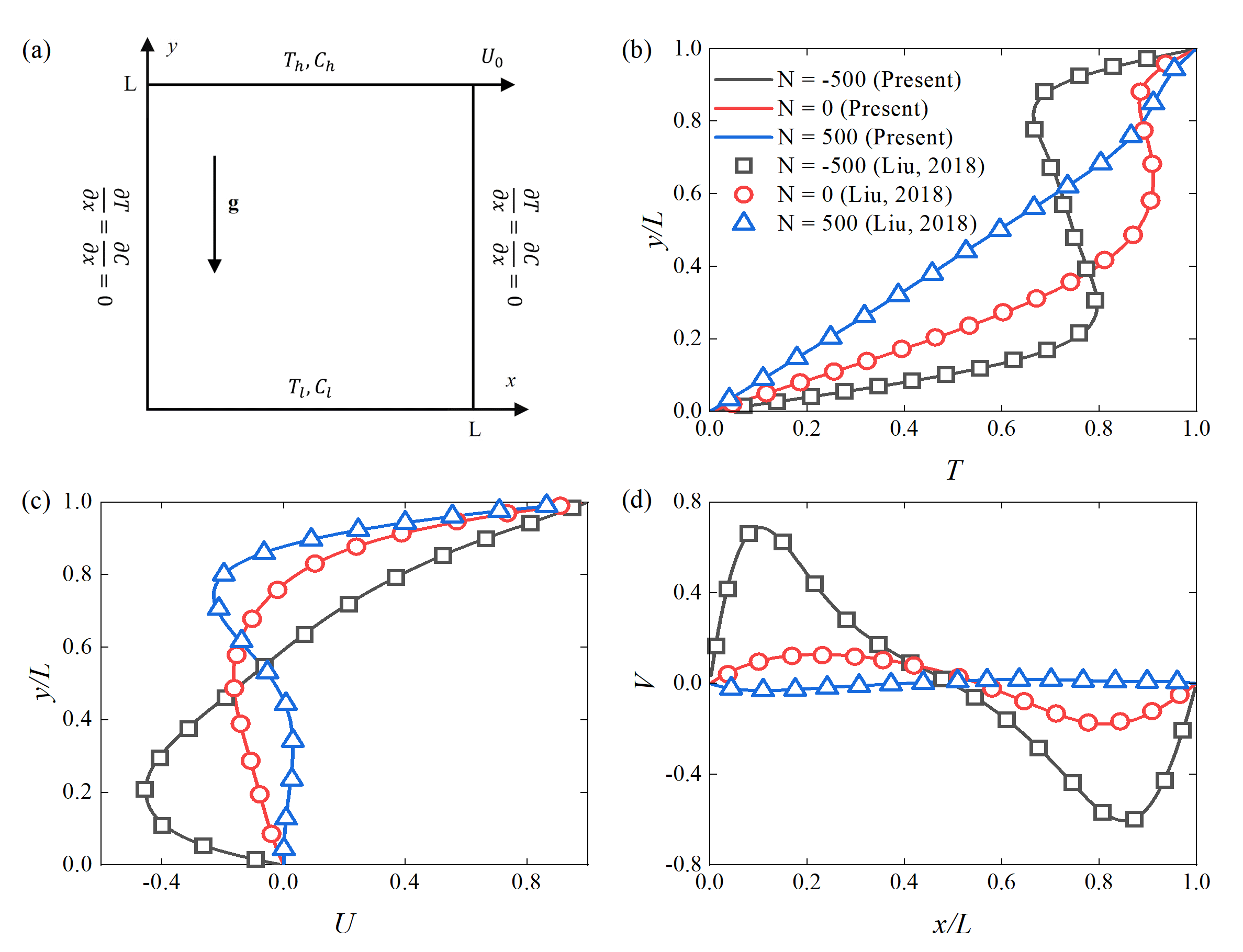
Figure 10: Validation of LBM framework on double-diffusive convection problem in porous media. (a) vertical temperature profile at x/L=0.5; (b) vertical velocity profile at x/L=0.5; (c) horizontal velocity profile at x/L=0.5. (b) vertical velocity on $y=0.5$, (c) temperature on $y=0.5$

Since the magnetic hyperthermia problem governed by Equation 1d actually can be viewed as a double-diffusive convection problem in porous media. Therefore, a typical porous double-diffusive convection validation is conducted to justify this framework. Figure 10 show the comparison on velocity and temperature with Reference [42] at various buoyancy ratio $N$. It is indicated that the present results match well with the reference.

Appendix B Implicit immersed boundary

Induced by the blood pulsation and deformable tissue domain, the vessel wall is regarded as a moving boundary. IBM is a mixed Eulerian–Lagrangian method by adding a force density term to satisfy the no-slip boundary condition. Generally, IBM can easily handle situations where the interface grids do not match in the Eulerian and Lagrangian configurations with desired numerical accuracy. In this research, a direct-forcing IBM scheme with the diffuse interface treatment is applied to simulate the movement of the blood vessel wall.

Based on the Lattice Boltzmann Equation 15, the boundary force in two-dimension at point $x_{b}$ is given by [55]

$$\mathbf{f}_{b}(s,t)=2\rho\frac{\mathbf{U}^{d}(s,t)-\mathbf{u}^{noF}(s,t)}{\delta t}$$ (25)

where $\mathbf{U}^{d}(s,t)$ and $\mathbf{u}^{noF}(s,t)$ are namely expected and unforced velocity on the Lagrangian coordinate, and unforced velocity is interpolated from the Eulerian configuration as

$$\mathbf{u}^{noF}(s,t)=\sum_{k}\mathbf{u}^{noF}(x_{k},t)D(x_{k}-x_{b}(s,t))h^{3}$$ (26)

and the unforced velocity $\mathbf{u}^{noF}(s,t)$ is collected from the particle distribution function in LB Equation without forcing term as

$$\mathbf{u}^{noF}(x_{k},t)=\frac{1}{\rho}\sum_{i}e_{i}f_{i}(x_{k},t)$$ (27)

Then the boundary force on the Eulerian configuration can interpolate from the Lagrangian coordinate as

$$\mathbf{F}_{b}(x_{k},t)=\sum_{b}\mathbf{f}_{b}(s,t)D(x_{k}-x_{b})\delta s_{b}$$ (28)

Finally, velocity on Eulerian configuration updates by

$$\mathbf{u}(x_{k},t)=\mathbf{u}^{noF}(x_{k},t)+\frac{\delta t}{2\rho}\mathbf{F}_{b}(x_{k},t)$$ (29)

To better satisfy the no-slip boundary condition, a new velocity is obtained by interpolating from $\mathbf{u}(x_{k},t)$ with Equation 26 to substitute $\mathbf{u}^{noF}(s,t)$, and then iterating the Equation 25, 28, 29, 26 until the difference between the updated velocity and the desired velocity is small enough.

In this process, $x_{k}$ is the independent Cartesian coordinates, while $s$ is the independent curvilinear coordinate. $h=\delta x_{k}$ denotes the meshing space and $\delta s_{b}$ is the segment length of boundary.

Delta function applied on interpolation is given by

$$D(x_{k}-x_{b})=\frac{1}{h^{2}}d(\frac{x_{k}-x_{b}}{h})d(\frac{y_{k}-y_{b}}{h})$$ (30)

where $d(r)$ is a weighting function defined as

$$d(r)=\begin{cases}\frac{1}{8}(3-2|r|+\sqrt{1+4|r|-4r^{2}})&|r|\leq 1\\ \frac{1}{8}(5-2|r|+\sqrt{-7+12|r|-4r^{2}})&1\leq|r|\leq 2\\ 0&|r|\geq 2\end{cases}$$ (31)

The cases of flow past the cylinder are applied on the validation of immersed boundary. The uniform flow past a fixed circular cylinder is studied. Flow is coming from the left boundary with the velocity $U_{\infty}$, and the homogeneous Neumann boundary is assigned at the right boundary. We compare two steady flow conditions ($Re=20$ and $40$, with $40D\times 40D$ computational domain) and two vortex shedding flow conditions ($Re=100$ and $150$, with $60D\times 40D$ computational domain). The results are listed in Table 10, and obviously match well with the reference.

Table 10: Validation of immersed boundary method on flow past cylinder case in [55]

Steady flow
Reynolds number	20				40
Parameters	$C_{D}$		$L_{w}$		$C_{D}$		$L_{w}$
Kang, 2010	2.119		1.033		1.584		2.486
Present	2.137		1.036		1.597		2.508
Unsteady flow
Reynolds number	100				150
Parameters	Avg. $C_{D}$	$C_{L}$		$St$	Avg. $C_{D}$	$C_{L}$		$St$
Kang, 2010	1.368	$\pm 0.346$		0.162	1.351	$\pm 0.542$		0.181
Present	1.381	$\pm 0.355$		0.164	1.367	$\pm 0.543$		0.181

Appendix C Blood rheology

Blood is a complex mixture of erythrocytes, leukocytes, thrombocytes, iron oxides, and other components suspended in plasma [30, 31], which makes the shear rate of blood fluid is not linearly related to the viscosity. Blood rheology can be regarded as a shear-rate-dependent non-Newtonian fluid [32]. Already some experiments and numerical studies reveal the rheological behavior of blood, and several shear-thinning models are accepted in the related works, such as Power-Law Model [56], Casson Model [57], and Carreua-Yasuda Model [58, 59, 60, 61, 62]. Since Carreua-Yasuda can describe a wild scope of blood flow and has been commonly applied for portraying the shear-shinning behavior of blood, which is selected in this research.

Generally, the Carreua-Yasuda Model is defined as

$$\eta=\eta_{\infty}+(\eta_{0}-\eta_{\infty})[1+(\lambda\dot{\gamma})^{a}]^{\frac{n-1}{a}}$$ (32)

where $\eta_{0}$ and $\eta_{\infty}$ are the viscosity at the zero shear rate and infinite shear rate, respectively. $n$ denotes the power-law exponent about the flow behavior. $a$ is the parameter controlling the width of the transition region. $\lambda$ is a time constant, whose inverse $\frac{1}{\lambda}$ denotes the position where the viscosity start to drop.

Shear rate $\dot{\gamma}$ is a relevant parameter to the second invariant of the rate-of-strain tensor and is defined as

$$\dot{\gamma}=\sqrt{\frac{1}{2}\Pi}=\sqrt{\frac{1}{2}[\sum_{i}\sum_{j}\dot{\gamma}_{ij}\dot{\gamma}_{ji}]}$$ (33)

and $\dot{\gamma}_{ij}$ is defined as

$$\dot{\gamma}_{ij}=u_{i,j}+u_{j,i}$$ (34)

To validate the blood rheology with Carreua-Yasuda Model, a lid-driven cavity flow field is adopted for comparison. As Figure 11 (a) illustrates, the upper wall moves with a constant velocity $U_{0}$, while the other three walls are fixed. Figure 11 (b) and (c) present the horizontal velocity at $x/L=0.5$ and vertical velocity at $y/L=0.5$, respectively, where the parameter $a$ (see Equation 32 varies from 0.2 to 10.0. According to the results, the velocity profiles match well with the reference.

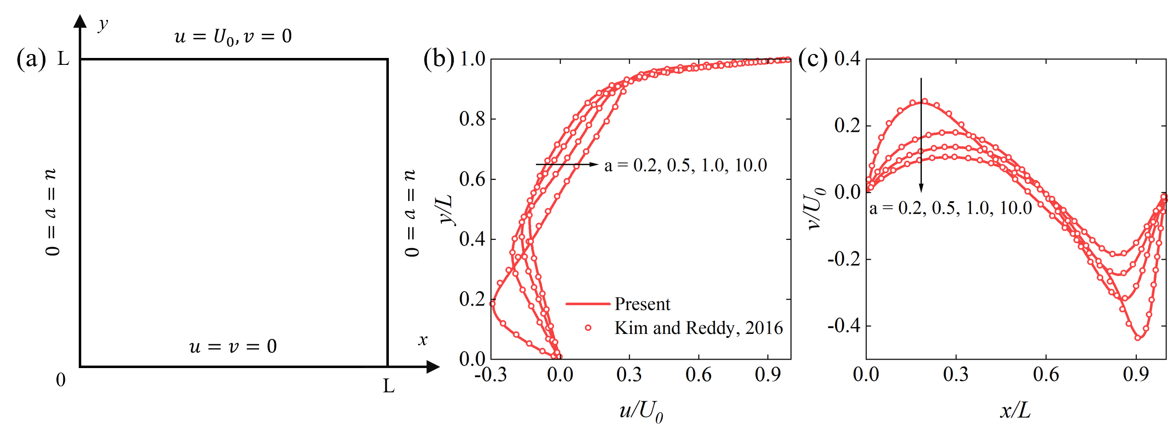
Figure 11: Validation of Carreua-Yasuda non-Newtonian Model on a lid-driven cavity flow field. (a) Schematic in [62]; (b) Horizontal velocity at $x/L=0.5$, and (c) Vertical velocity at $y/L=0.5$ with various values of $a$.

References

- [1] S. Sharma, N. Shrivastava, F. Rossi, N. T. K. Thanh, et al., Nanoparticles-based magnetic and photo induced hyperthermia for cancer treatment, Nano Today 29 (2019) 100795.
- [2] V. Vilas-Boas, F. Carvalho, B. Espiña, Magnetic hyperthermia for cancer treatment: main parameters affecting the outcome of in vitro and in vivo studies, Molecules 25 (12) (2020) 2874.
- [3] J. Ma, X. Yang, Y. Sun, J. Yang, Theoretical investigation on the thermo-mechanical responses of the human skin during thermal therapy, International Journal of Mechanical Sciences 161 (2019) 105041.
- [4] E. A. Périgo, G. Hemery, O. Sandre, D. Ortega, E. Garaio, F. Plazaola, F. J. Teran, Fundamentals and advances in magnetic hyperthermia, Applied Physics Reviews 2 (4) (2015) 041302.
- [5] J. Jose, R. Kumar, S. Harilal, G. E. Mathew, D. G. T. Parambi, A. Prabhu, M. Uddin, L. Aleya, H. Kim, B. Mathew, et al., Magnetic nanoparticles for hyperthermia in cancer treatment: an emerging tool, Environmental Science and Pollution Research 27 (16) (2020) 19214–19225.
- [6] D. Karponis, M. Azzawi, A. Seifalian, An arsenal of magnetic nanoparticles; perspectives in the treatment of cancer, Nanomedicine 11 (16) (2016) 2215–2232.
- [7] E. Kosari, K. Vafai, Transport and dynamic analysis of magnetic nanoparticles in brain microvascular vessels, Physics of Fluids 33 (8) (2021) 081907.
- [8] D. Chang, M. Lim, J. A. Goos, R. Qiao, Y. Y. Ng, F. M. Mansfeld, M. Jackson, T. P. Davis, M. Kavallaris, Biologically targeted magnetic hyperthermia: potential and limitations, Frontiers in pharmacology 9 (2018) 831.
- [9] M. Suto, Y. Hirota, H. Mamiya, A. Fujita, R. Kasuya, K. Tohji, B. Jeyadevan, Heat dissipation mechanism of magnetite nanoparticles in magnetic fluid hyperthermia, Journal of Magnetism and Magnetic Materials 321 (10) (2009) 1493–1496.
- [10] R. E. Rosensweig, Heating magnetic fluid with alternating magnetic field, Journal of magnetism and magnetic materials 252 (2002) 370–374.
- [11] I. Raouf, S. Khalid, A. Khan, J. Lee, H. S. Kim, M.-H. Kim, A review on numerical modeling for magnetic nanoparticle hyperthermia: Progress and challenges, Journal of thermal biology 91 (2020) 102644.
- [12] G. Singh, N. Kumar, P. K. Avti, Computational evaluation of effectiveness for intratumoral injection strategies in magnetic nanoparticle assisted thermotherapy, International Journal of Heat and Mass Transfer 148 (2020) 119129.
- [13] K. Mahmoudi, A. Bouras, D. Bozec, R. Ivkov, C. Hadjipanayis, Magnetic hyperthermia therapy for the treatment of glioblastoma: a review of the therapy’s history, efficacy and application in humans, International Journal of Hyperthermia 34 (8) (2018) 1316–1328.
- [14] A. Dahaghin, S. Emadiyanrazavi, M. Salimibani, H. Bahreinizad, M. Haghpanahi, R. Eivazzadeh-Keihan, A. Maleki, A numerical investigation into the magnetic nanoparticles hyperthermia cancer treatment injection strategies, Biocybernetics and Biomedical Engineering 41 (2) (2021) 516–526.
- [15] A. A. Golneshan, M. Lahonian, Diffusion of magnetic nanoparticles in a multi-site injection process within a biological tissue during magnetic fluid hyperthermia using lattice boltzmann method, Mechanics Research Communications 38 (6) (2011) 425–430.
- [16] C. Nicholson, Diffusion and related transport mechanisms in brain tissue, Reports on progress in Physics 64 (7) (2001) 815.
- [17] M. Roustaei, M. Servatkhah, Effect of mass transfer and diffusion on temperature distribution during magnetic hyperthermia, Physica B: Condensed Matter 631 (2022) 413498.
- [18] E. H. Ooi, E. T. Ooi, Mass transport in biological tissues: comparisons between single-and dual-porosity models in the context of saline-infused radiofrequency ablation, Applied Mathematical Modelling 41 (2017) 271–284.
- [19] M. Soltani, M. H. Tehrani, F. M. Kashkooli, M. Rezaeian, Effects of magnetic nanoparticle diffusion on microwave ablation treatment: A numerical approach, Journal of Magnetism and Magnetic Materials 514 (2020) 167196.
- [20] M. Salloum, R. Ma, D. Weeks, L. Zhu, Controlling nanoparticle delivery in magnetic nanoparticle hyperthermia for cancer treatment: experimental study in agarose gel, International Journal of Hyperthermia 24 (4) (2008) 337–345.
- [21] Y.-d. Tang, T. Jin, R. C. Flesch, Impact of different infusion rates on mass diffusion and treatment temperature field during magnetic hyperthermia, International Journal of Heat and Mass Transfer 124 (2018) 639–645.
- [22] Y.-d. Tang, T. Jin, R. C. Flesch, Effect of mass transfer and diffusion of nanofluid on the thermal ablation of malignant cells during magnetic hyperthermia, Applied Mathematical Modelling 83 (2020) 122–135.
- [23] K. Erbertseder, J. Reichold, B. Flemisch, P. Jenny, R. Helmig, A coupled discrete/continuum model for describing cancer-therapeutic transport in the lung, PLoS One 7 (3) (2012) e31966.
- [24] I. Astefanoaei, I. Dumitru, H. Chiriac, A. Stancu, Thermofluid analysis in magnetic hyperthermia using low curie temperature particles, IEEE Transactions on Magnetics 52 (7) (2016) 1–5.
- [25] M. Zakariapour, M. H. Hamedi, N. Fatouraee, Numerical investigation of magnetic nanoparticles distribution inside a cylindrical porous tumor considering the influences of interstitial fluid flow, Transport in Porous Media 116 (1) (2017) 251–274.
- [26] Y. Tang, J. Zou, R. C. Flesch, T. Jin, Backflow modeling in nanofluid infusion and analysis of its effects on heat induced damage during magnetic hyperthermia, Applied Mathematical Modelling 114 (2023) 583–600.
- [27] J. A. Pedersen, F. Boschetti, M. A. Swartz, Effects of extracellular fiber architecture on cell membrane shear stress in a 3d fibrous matrix, Journal of biomechanics 40 (7) (2007) 1484–1492.
- [28] A. AlAmiri, K. Khanafer, K. Vafai, Fluid-structure interactions in a tissue during hyperthermia, Numerical Heat Transfer, Part A: Applications 66 (1) (2014) 1–16.
- [29] B. Gheflati, N. Naghavi, Computational study of nanoparticle assisted hyperthermia in tumors embedded with large blood vessels, International Journal of Heat and Mass Transfer 151 (2020) 119415.
- [30] E. Tzirtzilakis, A mathematical model for blood flow in magnetic field, Physics of fluids 17 (7) (2005) 077103.
- [31] C.-H. Wang, J.-R. Ho, A lattice boltzmann approach for the non-newtonian effect in the blood flow, Computers & Mathematics with Applications 62 (1) (2011) 75–86.
- [32] Y. I. Cho, K. R. Kensey, Effects of the non-newtonian viscosity of blood on flows in a diseased arterial vessel. part 1: Steady flows, Biorheology 28 (3-4) (1991) 241–262.
- [33] M. Cinthio, A. R. Ahlgren, J. Bergkvist, T. Jansson, H. W. Persson, K. Lindstrom, Longitudinal movements and resulting shear strain of the arterial wall, American Journal of Physiology-Heart and Circulatory Physiology 291 (1) (2006) H394–H402.
- [34] M. W. Dewhirst, B. Viglianti, M. Lora-Michiels, M. Hanson, P. Hoopes, Basic principles of thermal dosimetry and thermal thresholds for tissue damage from hyperthermia, International journal of hyperthermia 19 (3) (2003) 267–294.
- [35] S. V. Spirou, M. Basini, A. Lascialfari, C. Sangregorio, C. Innocenti, Magnetic hyperthermia and radiation therapy: radiobiological principles and current practice, Nanomaterials 8 (6) (2018) 401.
- [36] S. K. Kandala, E. Liapi, L. L. Whitcomb, A. Attaluri, R. Ivkov, Temperature-controlled power modulation compensates for heterogeneous nanoparticle distributions: a computational optimization analysis for magnetic hyperthermia, International Journal of Hyperthermia (2018).
- [37] S. A. Sapareto, W. C. Dewey, Thermal dose determination in cancer therapy, International Journal of Radiation Oncology* Biology* Physics 10 (6) (1984) 787–800.
- [38] Q. Liu, Y.-L. He, Q. Li, W.-Q. Tao, A multiple-relaxation-time lattice boltzmann model for convection heat transfer in porous media, International Journal of Heat and Mass transfer 73 (2014) 761–775.
- [39] K. Mehmood, S. Hussain, M. Sagheer, Numerical simulation of mhd mixed convection in alumina–water nanofluid filled square porous cavity using kkl model: Effects of non-linear thermal radiation and inclined magnetic field, Journal of Molecular Liquids 238 (2017) 485–498.
- [40] S. Hussain, K. Mehmood, M. Sagheer, M. Yamin, Numerical simulation of double diffusive mixed convective nanofluid flow and entropy generation in a square porous enclosure, International Journal of Heat and Mass Transfer 122 (2018) 1283–1297.
- [41] Z. Guo, T. Zhao, Lattice boltzmann model for incompressible flows through porous media, Physical review E 66 (3) (2002) 036304.
- [42] Q. Liu, Y.-L. He, Multiple-relaxation-time lattice boltzmann model for simulating double-diffusive convection in fluid-saturated porous media, International Journal of Heat and Mass Transfer 127 (2018) 497–502.
- [43] J. Lang, B. Erdmann, M. Seebass, Impact of nonlinear heat transfer on temperature control in regional hyperthermia, IEEE Transactions on Biomedical Engineering 46 (9) (1999) 1129–1138.
- [44] J. Buongiorno, Convective transport in nanofluids, Journal of Heat Transfer (2006).
- [45] N. S. Gibanov, M. A. Sheremet, H. F. Oztop, O. K. Nusier, Convective heat transfer of ferrofluid in a lid-driven cavity with a heat-conducting solid backward step under the effect of a variable magnetic field, Numerical Heat Transfer, Part A: Applications 72 (1) (2017) 54–67.
- [46] H. Zhang, Lattice boltzmann method for solving the bioheat equation, Physics in Medicine & Biology 53 (3) (2008) N15.
- [47] M. A. Swartz, M. E. Fleury, Interstitial flow and its effects in soft tissues, Annu. Rev. Biomed. Eng. 9 (2007) 229–256.
- [48] P. Vennemann, R. Lindken, J. Westerweel, In vivo whole-field blood velocity measurement techniques, Experiments in fluids 42 (2007) 495–511.
- [49] Z. Wang, C. Wang, F. Zhao, N. Qi, D. Lockington, K. Ramaesh, P. S. Stewart, X. Luo, H. Tang, Simulation of fluid-structure interaction during the phaco-emulsification stage of cataract surgery, International Journal of Mechanical Sciences 214 (2022) 106931.
- [50] F. Ren, C. Wang, H. Tang, Active control of vortex-induced vibration of a circular cylinder using machine learning, Physics of Fluids 31 (2019) 093601.
- [51] C. Wang, H. Tang, F. Duan, C. Simon, Control of wakes and vortex-induced vibrations of a single circular cylinder using synthetic jets, Journal of Fluids and Structures 60 (2016) 160–179.
- [52] K. Das, S. C. Mishra, Estimation of tumor characteristics in a breast tissue with known skin surface temperature, Journal of thermal biology 38 (6) (2013) 311–317.
- [53] K. Das, R. Singh, S. C. Mishra, Numerical analysis for determination of the presence of a tumor and estimation of its size and location in a tissue, Journal of thermal biology 38 (1) (2013) 32–40.
- [54] P. Lallemand, L.-S. Luo, Theory of the lattice boltzmann method: Dispersion, dissipation, isotropy, galilean invariance, and stability, Physical review E 61 (6) (2000) 6546.
- [55] S. K. Kang, Immersed boundary methods in the lattice Boltzmann equation for flow simulation, Texas A&M University, 2010.
- [56] D. S. Loenko, A. Shenoy, M. A. Sheremet, Natural convection of non-newtonian power-law fluid in a square cavity with a heat-generating element, Energies 12 (11) (2019) 2149.
- [57] W. P. Walawender, T. Y. Chen, D. F. Cala, An approximate casson fluid model for tube flow of blood, Biorheology 12 (2) (1975) 111–119.
- [58] G. R. Kefayati, H. Tang, Three-dimensional lattice boltzmann simulation on thermosolutal convection and entropy generation of carreau-yasuda fluids, International Journal of Heat and Mass Transfer 131 (2019) 346–364.
- [59] G. R. Kefayati, Fdlbm simulation of magnetic field effect on non-newtonian blood flow in a cavity driven by the motion of two facing lids, Powder technology 253 (2014) 325–337.
- [60] G. R. Kefayati, H. Tang, Lattice boltzmann simulation of viscoplastic fluids on natural convection in an inclined enclosure with inner cold circular/elliptical cylinders (part i: One cylinder), International Journal of Heat and Mass Transfer 123 (2018) 1138–1162.
- [61] G. R. Kefayati, H. Tang, Double-diffusive natural convection and entropy generation of carreau fluid in a heated enclosure with an inner circular cold cylinder (part ii: Entropy generation), International Journal of Heat and Mass Transfer 120 (2018) 683–713.
- [62] N. Kim, J. Reddy, A spectral/hp least-squares finite element analysis of the carreau–yasuda fluids, International Journal for Numerical Methods in Fluids 82 (9) (2016) 541–566.