An Improved Kernel and Parameterized Algorithm for Almost Induced Matching

Abstract

An induced subgraph is called an induced matching if each vertex is a degree-1 vertex in the subgraph. The Almost Induced Matching problem asks whether we can delete at most $k$ vertices from the input graph such that the remaining graph is an induced matching. This paper studies parameterized algorithms for this problem by taking the size $k$ of the deletion set as the parameter. First, we prove a $6k$-vertex kernel for this problem, improving the previous result of $7k$. Second, we give an $O^{*}(1.6957^{k})$-time and polynomial-space algorithm, improving the previous running-time bound of $O^{*}(1.7485^{k})$.

Keywords

Graph Algorithms, Maximum Induced Matching, Parameterized Algorithms, Linear Kernel

1 Introduction

An induced matching is an induced regular graph of degree 1. The problem of finding an induced matching of maximum size is known as Maximum Induced Matching (MIM), which is crucial in algorithmic graph theory. In many graph classes such as trees [6], chordal graphs [2], circular-arc graphs [5], and interval graphs [6], a maximum induced matching can be found in polynomial time. However, Maximum Induced Matching is NP-hard in planar 3-regular graphs or planar bipartite graphs with degree-2 vertices in one part and degree-3 vertices in the other part [4, 10, 17]. Kobler and Rotics [11] proved the NP-hardness of this problem in Hamiltonian graphs, claw-free graphs, chair-free graphs, line graphs, and regular graphs. The applications of induced matchings are diverse and include secure communication channels, VLSI design, and network flow problems, as demonstrated by Golumbic and Lewenstein [6].

In terms of exact algorithms, Gupta, Raman, and Saurabh [7] demonstrated that Maximum Induced Matching can be solved in $O^{*}(1.6957^{n})$ time. This result was later improved to $O^{*}(1.3752^{n})$ by Xiao and Tan [19]. For subcubic graphs (i.e., such graphs with maximum degree $3$), Hoi, Sabili and Stephan [8] showed that Maximum Induced Matching can be solved in $O^{*}(1.2630^{n})$ time. In terms of parameterized algorithms, where the parameter is the solution size $k^{\prime}$, Maximum Induced Matching is W[1]-hard in general graphs [16], and is not expected to have a polynomial kernel. However, Moser and Sidkar [15] showed that the problem becomes fixed-parameter tractable (FPT) when the graph is a planar graph, by providing a linear-size problem kernel. The kernel size was improved to $40k^{\prime}$ by Kanj et al. [9]. In this paper, we study parameterized algorithms for Maximum Induced Matching by considering another parameter. Specifically, we take the number $k$ of vertices not in the induced matching as our parameter. The problem is formally defined as follows:

  Almost Induced Matching
Instance: A graph $G=(V,E)$ and an integer $k$.
Question: Is there a vertex subset $S\subseteq V$ of size at most $k$ whose deletion makes the graph an induced matching?
 

Almost Induced Matching becomes FPT when we take the size $k$ of the deletion set as the parameter. Xiao and Kou [18] showed that Almost Induced Matching can be solved in $O^{*}(1.7485^{k})$. The same running time bound was also achieved in [13] recently. In terms of kernelization, Moser and Thilikos [16] provided a kernel of $O(k^{3})$ vertices. Then, Mathieson and Szeider [14] improved the result to $O(k^{2})$. Last, Xiao and Kou [18] obtained the first linear-vertex kernel of $7k$ vertices for this problem. In this paper, we first give an $O^{*}(1.6957^{k})$-time and polynomial-space algorithm for Almost Induced Matching and then improve the kernel size to $6k$ vertices.

Our parameterized algorithm is a branch-and-search algorithm that adopts the framework of the algorithm in the previous paper [18]. We first handle vertices with degrees of 1 and 2, followed by those with degree at least 5. The different part is that we use refined rules to deal with degree-3 and degree-4 vertices, which can avoid the previous bottleneck. As for kernelization, the main technique in this paper is a variant of the crown decomposition. We find a maximal 3-path packing $\mathcal{P}$ in the graph, partition the vertex set into two parts $V(\mathcal{P})$ and $Q=V\setminus V(\mathcal{P})$, and reduce the number of the size-1 connected components of $G[Q]$ to at most $k$. The size-2 components in $G[Q]$ can be reduced to at most $k$ by using the new “AIM crown decomposition” technique. Note that each connected component of $G[Q]$ has a size of at most $2$. The size of $\mathcal{P}$ is at most $k$ since at least one vertex must be deleted from each $3$-path. In the worst case scenario, when there are $k$ 3-paths in $\mathcal{P}$, $k$ size-2 components, and $k$ size-1 components in $G[Q]$, the graph has at most $3k+2k+k=6k$ vertices.

2 Preliminaries

In this paper, we only consider simple and undirected graphs. Let $G=(V,E)$ be a graph with $n=|V|$ vertices and $m=|E|$ edges. A singleton $\{v\}$ may be denoted as $v$. We use $V(G^{\prime})$ and $E(G^{\prime})$ to denote the vertex set and edge set of a graph $G^{\prime}$, respectively. A vertex $v$ is called a neighbor of a vertex $u$ if there is an edge $\{u,v\}\in E$. Let $N(v)$ denote the set of neighbors of $v$. For a vertex subset $X$, let $N(X)=\cup_{v\in X}N(v)\setminus X$ and $N[X]=N(X)\cup X$. We use $d(v)=|N(v)|$ to denote the degree of a vertex $v$ in $G$. A vertex of degree $d$ is called a degree-$d$ vertex. For a vertex subset $X\subseteq V$, the subgraph induced by $X$ is denoted by $G[X]$, and $G[V\setminus X]$ is also written as $G\setminus X$ or $G-X$. A vertex in a vertex subset $X$ is called an $X$-vertex. Two vertex-disjoint subgraphs $X_{1}$ and $X_{2}$ are adjacent if there is an edge $\{u,v\}\in E$ with $u\in X_{1}$ and $v\in X_{2}$. A graph is called an induced matching if the size of each connected component in it is two. A vertex subset $S$ is called an AIM-deletion set of $G$ if $G\setminus S$ is an induced matching.

A $3$-path $P_{3}=\{u_{1},u_{2},u_{3}\}$ is a path with two edges $\{u_{1},u_{2}\}$ and $\{u_{2},u_{3}\}\in E$. Two $3$-paths $L_{1}$ and $L_{2}$ are vertex-disjoint if $V(L_{1})\cap V(L_{2})=\emptyset$. A set of 3-paths $\mathcal{P}=\{L_{1},L_{2},...,L_{t}\}$ is called a $P_{3}$-packing if any two 3-paths in it are vertex-disjoint. A $P_{3}$-packing is maximal if there is no $P_{3}$-packing $\cal P^{\prime}$ such that $|\mathcal{P}|<|\mathcal{P^{\prime}}|$ and $\mathcal{P}\subseteq\mathcal{P^{\prime}}$. We use $V(\mathcal{P})$ to denote the set of vertices in 3-paths in $\mathcal{P}$.

The classic crown decomposition technique, called VC crown decomposition, is originally introduced for the Vertex Cover problem [1, 3]. In this paper, we will use a variant of it. We first give the definition of VC crown decomposition for the ease of reference.

Definition 1.

A VC crown decomposition of a graph $G=(V,E)$ is a partition $(C,H,R)$ of the vertex set $V$ satisfying the following properties.

1. There is no edge between $C$ and $R$.

2. $C$ is an independent set.

3. There is an injective mapping (matching) $M:H\rightarrow C$ such that $\{x,M(x)\}\in E$ holds for all $x\in H$.

Lemma 1 ([3]).

If graph $G=(V,E)$ has an independent set $I\subseteq V$ with $|I|>|N(I)|$, then a VC crown decomposition $(C,H,R)$ with $\emptyset\neq C\subseteq I$ and $H\subseteq N(I)$ can be found in linear time.

3 Kernelization

In this section, we show that Almost Induced Matching allows a kernel of $6k$ vertices. The main idea of our algorithm is as follows. The first step of this algorithm is to find a maximal $P_{3}$-packing $\mathcal{P}$ in $G=(V,E)$ by using a greedy method. Then we use a method in [18] to update $\mathcal{P}$ to satisfy some properties. Since we need to delete at least one vertex in each 3-path, the instance is a yes-instance only if $|\mathcal{P}|\leq k$. We partition the vertex set $V$ into two parts $P=V(\mathcal{P})$ and $Q=V\setminus P$. Each connected component in $G[Q]$ is of size at most 2 by the maximality of $\mathcal{P}$. We will bound the number of components in $G[Q]$ to bound the size of $Q$.

Let $Q_{0}$ denote the set of degree-0 vertices in $G[Q]$, and $Q_{1}$ denote the set of degree-1 vertices in $G[Q]$. Use $Q_{1}$-edge to denote the components with size 2 in $G[Q]$. For each $L_{i}\in\mathcal{P}$, let $Q(L_{i})$ denote the set of $Q$-vertices in the components of $G[Q]$ adjacent to $L_{i}$. Let $V_{i}$ denote $Q(L_{i})\cup V(L_{i})$. It should be noted that a vertex in $Q(L_{i})$ might not have a direct connection to any vertex in $L_{i}$.

A 3-path $L_{i}\in\mathcal{P}$ is good if at most one vertex in $L_{i}$ is adjacent to $Q$-vertices. A 3-path $L_{i}\in\mathcal{P}$ is bad if at least two vertices in $L_{i}$ are adjacent to $Q$-vertices. A maximal $P_{3}$-packing is proper if for any bad 3-path $L_{i}\in\mathcal{P}$, it holds that $|V_{i}|\leq 6$.

After obtaining an arbitrary maximal $P_{3}$-packing $\mathcal{P}$, we use two rules in [18] to update $\mathcal{P}$.

Rule 1 ([18]).

If there is a 3-path $L_{i}\in\mathcal{P}$ such that $G[V_{i}]$ contains at least two vertex-disjoint 3-paths, then replace $L_{i}$ by these 3-paths in $\mathcal{P}$ to increase the size of $\mathcal{P}$ by at least one.

Lemma 2 ([18]).

Assume that Rule 1 can not be applied on the current instance. For any $L_{i}\in\mathcal{P}$ with $|V_{i}|\geq 7$, there is a 3-path $L^{\prime}_{i}$ in $G[V_{i}]$ such that $L^{\prime}_{i}$ is a good 3-path after replacing $L_{i}$ with $L^{\prime}_{i}$ in $\mathcal{P}$. Furthermore, the 3-path $L^{\prime}_{i}$ can be found in constant time.

We call the 3-path $L^{\prime}_{i}$ in Lemma 2 a quasi-good 3-path.

Rule 2 ([18]).

For any 3-path $L_{i}\in\mathcal{P}$ with $|V_{i}|\geq 7$, if it is not good, then replace $L_{i}$ with a quasi-good 3-path $L^{\prime}_{i}$ in $\mathcal{P}$.

Lemma 3 ([18]).

For any initially maximal $P_{3}$-packing $\mathcal{P}$ in $G$, we can apply Rules 1 and 2 in $O(n^{2})$ time to change $\mathcal{P}$ to a proper $P_{3}$-packing.

This lemma implies that the number of $Q$-vertices in the components of $G[Q]$ adjacent to bad 3-paths in $\mathcal{P}$ is small. So we only need to bound the number of $Q_{0}$-vertices and $Q_{1}$-edges adjacent to good 3-paths in $\mathcal{P}$. For any proper $P_{3}$-packing $\mathcal{P}$ in $G$, we can bound the number of $Q_{0}$-vertices adjacent to good 3-paths by the following Lemma 4 from [18].

Lemma 4 ([18]).

Let $\mathcal{P}$ be a proper $P_{3}$-packing in graph $G$, where the number of bad 3-paths is $x$. If $(G,k)$ is a yes-instance, then the number of $Q_{0}$-vertices only adjacent to good 3-paths (not adjacent to bad 3-paths) in $\mathcal{P}$ is at most $k-x$.

The main contribution in this paper is to bound the number of $Q_{1}$-edges adjacent to good 3-paths. We need to use the following technique called AIM crown decomposition.

Definition 2 (AIM crown decomposition).

An AIM crown decomposition of a graph $G=(V,E)$ is a decomposition $(C,H,R)$ of the vertex set $V$ such that

1. there is no edge between $C$ and $R$;

2. the induced subgraph $G[C]$ is an induced matching;

3. there is an injective mapping (matching from vertices to edges) $M:H\rightarrow E(C)$ such that for all $v\in H$, there exists $u\in M(v)$ such that $(u,v)\in E$.

Fig. 1 illustrates an AIM crown decomposition. We have the following lemma for AIM crown decomposition, which allows us to find parts of the solution based on an AIM crown decomposition.

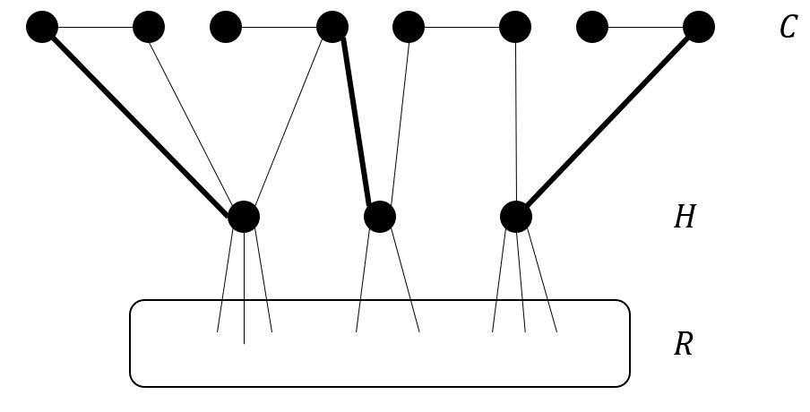
Figure 1: An AIM crown decomposition $(C,H,R)$, where the three bold edges form an injective matching from $H$ to $C$.

Lemma 5.

Let $(C,H,R)$ be an AIM crown decomposition of a graph $G$. There is a minimum AIM-deletion set $S$ such that $H\subseteq S$.

Proof.

Let $S^{*}$ be an arbitrary minimum AIM-deletion set of $G$. Let $G^{\prime}=G\setminus S^{*}$. Note that $G^{\prime}$ is an induced matching. We partition $H$ into two sets $H_{1}$ and $H_{2}$, where $H_{1}=H\cap S^{*}$ and $H_{2}=H\setminus H_{1}$. So all vertices in $H_{2}$ are in the induced matching $G^{\prime}$. We further partition $H_{2}$ into two sets $H_{C}$ and $H_{R}$, where each vertex in $H_{C}$ is adjacent to a vertex in $C\cup H$ in the induced matching $G^{\prime}$ and each vertex in $H_{R}$ is adjacent to a vertex in $R$ in the induced matching $G^{\prime}$. Let $N_{G\setminus S^{*}}(H_{R})$ be the set of vertices adjacent to vertices in $H_{R}$ in the induced matching $G^{\prime}$.

We partition $C$ into two sets $C_{1}$ and $C_{2}$, where two vertices of each edge in $C_{1}$ are both in $G^{\prime}$ and $C_{2}=C\setminus C_{1}$. Let $T=H_{2}\cup C_{2}\cup N_{G\setminus S^{*}}(H_{R})$. See Fig. 2 for an illustration.

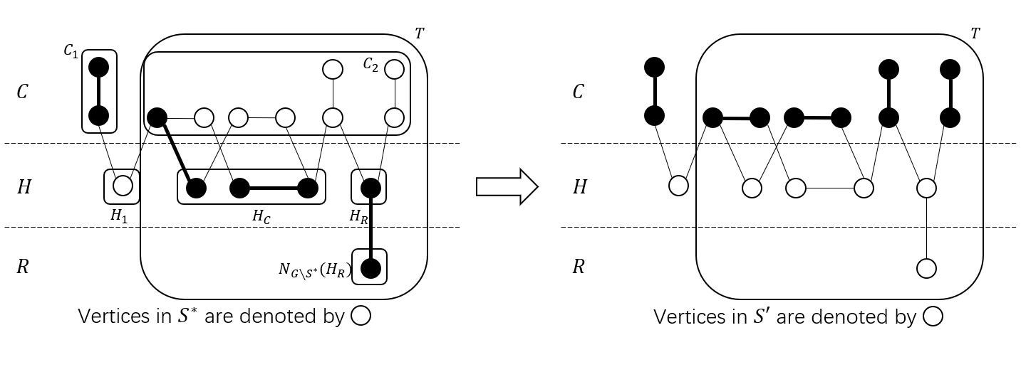
Figure 2: Sets $S^{*}$ and $S^{\prime}$ in the proof of Lemma 5.

Let $S^{\prime}=(S^{*}\setminus C)\cup H_{2}\cup N_{G\setminus S^{*}}(H_{R})$. Firstly, we show that $S^{\prime}$ is still an AIM-deletion set of $G$. See Fig. 2 for an illustration of $S^{*}$ and $S^{\prime}$. It is easy to see that $H\subseteq S^{\prime}$.

Let $S_{1}=S^{*}\setminus(H\cup C)$. We can see that $S_{1}$ is an AIM-deletion set of the induced subgraph $G\setminus(H\cup C\cup N_{G\setminus S^{*}}(H_{R}))$ by definition of $S^{*}$ and $N_{G\setminus S^{*}}(H_{R})$. So $S_{1}\cup H\cup N_{G\setminus S^{*}}(H_{R})$ is an AIM-deletion of origin graph $G$. We can see that $S_{1}\cup H\cup N_{G\setminus S^{*}}(H_{R})=S^{\prime}$. Then, we show that $|S^{\prime}|\leq|S^{*}|$ to finish our proof.

By definition of $S^{\prime}$, we have that

$$|S^{\prime}|=|S^{*}|-|S^{*}\cap C|+|H_{2}|+|N_{G\setminus S^{*}}(H_{R})|.$$ (1)

Note that, $H_{2}\cap S^{*}=\emptyset,N_{G\setminus S^{*}}(H_{R})\cap S^{*}=\emptyset,C_{1}\cap S^{*}=\emptyset$ because of their definitions. We have that

$$|S^{*}\cap T|=|S^{*}\cap C_{2}|=|S^{*}\cap C|.$$ (2)

Recall the definition of $T=H_{2}\cup C_{2}\cup N_{G\setminus S^{*}}(H_{R})$. Since $H$ is an $C$-$R$ cutset, vertices in $C_{2}$ can not be adjacent to $V\setminus T$ in $G^{\prime}$, and $H_{2},N_{G\setminus S^{*}}(H_{R})$ can not be adjacent to $V\setminus T$ in $G^{\prime}$ by their definitions. We can claim that there are at most $|H_{2}|$ induced matchings in $G^{\prime}[T\setminus S^{*}]$. We get that

$$|S^{*}\cap T|\geq|T|-2|H_{2}|.$$ (3)

Note that all edges in $C$ adjacent to $H_{2}$ must be in $C_{2}$, so we have $\forall v\in H_{2},M(v)\in C_{2}$, so $|C_{2}|\geq|H_{2}|,|V(C_{2})|\geq 2|H_{2}|$. By the definition of $T$, we have that

$$|H_{2}|+|N_{G\setminus S^{*}}(H_{R})|=|T|-|V(C_{2})|\leq|T|-2|H_{2}|.$$ (4)

Equality (2) with inequalities (3) and (4) together imply that

$$|H_{2}|+|N_{G\setminus S^{*}}(H_{R})|\leq|S^{*}\cap C|.$$ (5)

Equality (1) with inequality (5) together imply that

$$|S^{\prime}|=|S^{*}|-|S^{*}\cap C|+|H_{2}|+|N_{G\setminus S^{*}}(H_{R})|\leq|S^{*}|-|S^{*}\cap C|+|S^{*}\cap C|=|S^{*}|.$$

∎

Once given an AIM crown decomposition $(C,H,R)$ of the graph, we can reduce the instance by including $H$ to the deletion set and removing $H\cup C$ from the graph by Lemma 5. Next, we show that when the number of $Q_{1}$-edges is large we always find an AIM crown decomposition in polynomial time.

Lemma 6.

Let $G=(V,E)$ be a graph with each connected component containing more than two vertices, and $A$ and $B\subseteq V$ be two disjoint vertex sets such that
(i) no vertex in $A$ is adjacent to a vertex in $V\setminus(A\cup B)$;
(ii) the induced subgraph $G[A]$ is an induced matching.
If $|A|>2|B|$, then the graph allows an AIM crown decomposition $(C,H,R)$ with $\emptyset\neq C\subseteq A$ and $H\subseteq B$, and the AIM crown decomposition $(C,H,R)$ can be found in polynomial time.

Proof.

Firstly, we construct an auxiliary bipartite graph $G^{\prime}=(V^{\prime},E^{\prime})$ with $V^{\prime}=(A^{\prime},B^{\prime})$ as follows: Each vertex in $A^{\prime}$ corresponds to a component (an edge) in the induced matching $G[A]$, and each vertex in $B^{\prime}$ corresponds to a vertex in the vertex set $B$. And a vertex $a\in A_{H}$ is adjacent to a vertex $b\in B_{H}$ if and only if the component in $G[A]$ corresponding to $a$ is adjacent to the vertex $b$ in $G$. Note that $2|A^{\prime}|=|A|$ and $|B^{\prime}|=|B|$. If $|A|>2|B|$, then $|A^{\prime}|>|B^{\prime}|$.

Since the induced subgraph $G[A]$ is an induced matching, $G^{\prime}[A^{\prime}]$ is an independent set. Hence $G^{\prime}$ has a VC crown decomposition $(C^{\prime},H^{\prime},R^{\prime})$ with $C^{\prime}\subseteq A^{\prime}$ that can be found in linear time by Lemma 1.

Associate $(C^{\prime},H^{\prime},R^{\prime})$ to the decomposition $(C,H,R)$ of $V$, where $C$ is the components corresponding to the vertices in $C^{\prime}$, $H$ is the vertices corresponding to the vertices in $H^{\prime}$, $R=V\setminus(H\cup C)$. Let us check the three conditions in the definition of AIM crown decomposition in $(C,H,R)$.

1. Since there is no edge between $C^{\prime}$ and $R^{\prime}$, there is no edge between $C$ and $R$.

2. Since $C$ is an independent set, the induced subgraph $G[C]$ is an induced matching

3. Since there is an injective mapping (matching) $M^{\prime}:H^{\prime}\rightarrow C^{\prime}$ such that, $\forall x\in H^{\prime},\{x,M^{\prime}(x)\}\in E$, there is an injective mapping (matching from vertices to edges) $M:H\rightarrow E(C)$ such that for all $v\in H$, there exists $u\in M(v)$ such that $(u,v)\in E$ by transforming the vertices in $M^{\prime}$ into the corresponding vertices or edges in $V$.

Since $C^{\prime}\neq\emptyset$, we can say $C\neq\emptyset$. So $(C,H,R)$ is an AIM crown decomposition of $V$ with $\emptyset\neq C\subseteq A$ and $H\subseteq B$, and this decomposition can be found in polynomial time. ∎

If the number of $Q_{1}$-edges only adjacent to vertices of good 3-paths in $\mathcal{P}$ is large, we use Lemma 5 and Lemma 6 to reduce the instance. Our algorithm first finds two vertex-disjoint sets of vertices, $A$ and $B$, which satisfy the condition in Lemma 6 based on a proper $P_{3}$-packing $\mathcal{P}$. Let $A$ be the set of $Q_{1}$-vertices that are only adjacent to good 3-paths in $\mathcal{P}$. Let $B$ be the set of vertices in good 3-paths that are adjacent to some vertices in $A$. If $|A|>2|B|$, we can find an AIM crown decomposition $(C,H,R)$ by Lemma 6, and we can reduce the instance by including $C$ to the deletion set and removing $C\cup H$ from the graph.

Our algorithm, denoted by ${\tt Reduce}(G,k)$ is described in Fig. 3.

 
Input: An undirected graph $G=(V,E)$ and an integer $k$.
Output: An equivalent instance $(G^{\prime},k^{\prime})$ with $|V(G^{\prime})|\leq 6k^{\prime}$ and $k^{\prime}\leq k$ or no.

1. If there is a connected component $C$ of two vertices, return ${\tt Reduce}(G\setminus C,k)$.

2. If there is a connected component $C$ of one vertice, return ${\tt Reduce}(G\setminus C,k-1)$.

3. Find an arbitrary maximal $P_{3}$-packing $\mathcal{P}$ in $G$ by using greedy algorithm.

4. Iteratively apply Rules 1 and 2 to update $\mathcal{P}$ until none of them can be applied anymore.

5. If $|\mathcal{P}|>k$, then return ‘no’.

6. Let $P=V(\mathcal{P})$ and $Q=V\setminus P$.

7. If the number of $Q_{0}$-vertices only adjacent to good 3-paths is more than $k-x$, where $x$ is the number of bad 3-paths in $\mathcal{P}$, then return ‘no’.

8. Let $A$ be the set of $Q_{1}$-vertices that are only adjacent to good 3-paths in $\mathcal{P}$. Let $B$ be the set of vertices in good 3-paths that are adjacent to some vertices in $A$.

9. If $|A|>2|B|$, find an AIM crown decomposition $(C,H,R)$ by Lemma 6, return ${\tt Reduce}(G\setminus(C\cup H),k-|H|)$.

10. return $(G,k)$.

 

Figure 3: Algorithm ${\tt Reduce}(G,k)$

Lemma 7.

Algorithm ${\tt Reduce}(G,k)$ runs in polynomial time, and returns either an equivalent instance $(G^{\prime},k^{\prime})$ with $|V(G^{\prime})|\leq 6k^{\prime}$ and $k^{\prime}\leq k$ or no to indicate that the instance is a no-instance.

Proof.

First, let us consider the correctness of each step. Steps 1-6 are trivial cases. Step 7 is based on Lemma 4 and Step 9 is based on Lemma 5. Step 8 is also trivial. Next, we consider Step 10. In this step, $\mathcal{P}$ is a proper $P_{3}$-packing and then the number of vertices in $P$ is at most $3k$. Assume that the number of bad 3-paths in $\mathcal{P}$ is $x$ and the number of good 3-paths in $\mathcal{P}$ is $y$. By the definition of proper $P_{3}$-packing, we know that the number of vertices in bad 3-paths and in $Q$-components adjacent to some bad 3-paths is at most $6x$. The number of vertices in good 3-paths is $3y$, the number of $Q_{0}$ -vertices only adjacent to good 3-paths is at most $k-x$ by Lemma 4, and the number of $Q_{1}$-vertices only adjacent to good 3-paths is at most $2y$ by Lemma 5 and Lemma 6. In total, the number of vertices in the graph is at most $6x+3y+(k-x)+2y=k+5x+5y\leq 6k$. Thus, we can get that $|V|\leq 6k$ in Step 10.

Each step in ${\tt Reduce}(G,k)$ runs in polynomial time. Since each recursive call of ${\tt Reduce}(G,k)$ decreases $|V|$ by at least 1, ${\tt Reduce}(G,k)$ will be called at most $|V|$ times. Thus, ${\tt Reduce}(G,k)$ runs in polynomial time. ∎

Theorem 3.1.

Almost Induced Matching admits a kernel with $6k$ vertices.

4 A parameterized algorithm

In this section, we design a parameterized algorithm for Almost Induced Matching. Our algorithm is a branch-and-search algorithm that runs in $O^{*}(1.6957^{k})$ time and polynomial space. The branching operations in the algorithm determine the exponential component of the running time in branch-and-search algorithms. During a branching operation, the algorithm solves the current instance by solving multiple smaller instances. We use a parameter $k$ to measure the instance, and $T(k)$ to denote the maximum size of the searching tree generated by the algorithm when running on an instance with the parameter no greater than $k$. We can solve the instance in linear time when $k\leq 0$. If a branching operation generates $l$ branches and the measure $k$ in the $i$-th instance decreases by at least $c_{i}$, then this operation generates a recurrence relation

$$T(k)\leq T(k-c_{1})+T(k-c_{2})+...+T(k-c_{l})+1.$$

The largest root of the function $f(x)=1-\sum_{i=1}^{l}x^{-c_{i}}$ is called the branching factor of the recurrence. Let $\gamma$ denote the maximum branching factor among all branching factors. The running time of the algorithm is bounded by $O^{*}(\gamma^{k})$. Further information regarding the analysis and the solution of recurrences is available in the monograph [12].

4.1 Branching rules

For any vertex $v$, it is either in the deletion set or remains in the induced matching. If $v$ is included in the deletion set, we simply delete $v$ from the graph and add $v$ to the deletion set. If $v$ remains in the induced matching, it must be adjacent to one of its neighbors, which we denote as $u$. We then add all vertices in $N(\{u,v\})$ to the deletion set and delete all vertices in $N[\{u,v\}]$ from the graph. So we get the following simple branching rule.

Branching-Rule 1.

Branch on $v$ to generate $|N[v]|$ branches by either (i) deleting $v$ from the graph and including it in the deletion set, or (ii) for each neighbor $u$ of $v$, deleting $N[\{u,v\}]$ from the graph and including $N(\{u,v\})$ in the deletion set.

When dealing with certain graph structures, we can use a more effective branching rule. A vertex $v$ dominates its neighbor $u$ if $N[u]\subseteq N[v]$. A vertex $v$ is called a dominating vertex if it dominates at least one vertex. The following property of dominating vertices has been used in [7, 19].

Lemma 8.

Let $v$ be a vertex that dominates a vertex $u$. If there is a maximum induced matching $M$ of $G$ such that $v\in V(M)$, then there is a maximum induced matching $M^{\prime}$ of $G$ such that edge $vu\in M^{\prime}$.

We can use Lemma 8 to design an effective branching rule. Assume that $v$ dominates $u$. Vertex $v$ is either in the deletion set or remains in the induced matching with vertex $u$ by Lemma 8. We get the following branching rule.

Branching-Rule 2.

Assume that vertex $v$ dominates vertex $u$. Branch on $v$ to generate two instances by either (i) deleting $v$ from the graph and including it in the deletion set, or (ii) deleting $N[\{u,v\}]$ from the graph and including $N(\{u,v\})$ in the deletion set.

4.2 The algorithm

We will use ${\tt aim}(G,k)$ to denote our parameterized algorithm. Before executing the main branching steps, the algorithm will first apply some reduction rules to simplify the instance. First of all, we call the kernel algorithm ${\tt Reduce}(G,k)$ to reduce the instance, which can be considered as Reduction-Rule 0. We also have two more reduction rules.

Reduction-Rule 1.

If there is a connected component of the graph such that each vertex in it is a degree-2 vertex, then select an arbitrary vertex $v$ in this component and return ${\tt aim}(G\setminus\{v\},k-1)$.

Reduction-Rule 2.

If there is a degree-1 vertex $v$ with a degree-2 neighbor $u$, then return ${\tt aim}(G\setminus N[\{v,u\}],k-1)$.

Reduction-Rule 2 was proved and used in [18]. Its correctness is based on the observation: there is always a maximum induced matching containing edge $vu$.

Now, we are ready to introduce the main branching steps of the algorithm. The algorithm contains eight steps to handle different local structures of the graph. Dominating vertices are processed in Step 1, while Steps 2 to 4 are dedicated to handling degree-2 vertices. High degree vertices with at least five neighbors are handled in Step 5, and the last three steps focus on graphs with only degree-3/4 vertices. When executing a step, we assume that all previous steps are not applicable to the current graph.

The first five steps are adopted from [18].

Step 1 (Dominating vertices of degree $\geq 3$). If there is a vertex $v$ of degree $\geq 3$ that dominates a vertex $u$, then branch on $v$ with Rule (B2) to generate two branches.

$${\tt aim}(G\setminus\{v\},k-1)\quad\mbox{and}\quad{\tt aim}(G\setminus N[\{v,u\}],k-|N(\{v,u\})|).$$

Lemma 8 guarantees the correctness of this step. Note that $|N(\{v,u\})|$ = $d(v)-1$. This step generates a recurrence

$$T(k)\leq T(k-1)+T(k-(d(v)-1))+1,$$

where $d(v)\geq 3$. For the worst case where $d(v)=3$, the branching factor of it is 1.6181.

After Reduction-Rule 2, the degree-1 vertices can only be adjacent to the vertex of degree $\geq 3$. These vertices will be handled in Step 1. So after Step 1, there are no degree-1 vertices in $G$.

Next, we consider degree-2 vertices. A path $u_{0}u_{1}u_{2}u_{3}u_{4}$ of five vertices is called a chain if the first vertex $u_{0}$ is of degree $\geq 3$ and the three middle vertices are of degree 2, where we allow $u_{4}$ = $u_{0}$. A path $u_{0}u_{1}u_{2}u_{3}$ of four vertices is called a short chain if the first vertex $u_{0}$ and last vertex $u_{3}$ are of degree $\geq 3$ and the two middle vertices are of degree 2, where we allow $u_{3}$ = $u_{0}$. A chain or a short chain can be found in linear time if it exists.

Step 2 (Chains). If there is a chain $u_{0}u_{1}u_{2}u_{3}u_{4}$, then branch on $u_{1}$ with Rule (B1). In the branch where $u_{1}$ is deleted and included in the deletion set, we get a tail $u_{2}$ and then further deal with the tail as we do in Reduction-Rule 2. Then we get the following three branches

$$\begin{split}{\tt aim}(G\setminus\{u_{1},u_{2},u_{3},u_{4}\},k-2),&\quad{\tt aim}(G\setminus N[\{u_{0},u_{1}\}],k-|N(\{u_{0},u_{1}\})|),\\ \mbox{and}&\quad{\tt aim}(G\setminus N[\{u_{1},u_{2}\}],k-|N(\{u_{1},u_{2}\})|).\end{split}$$

The corresponding recurrence is

$$T(k)\leq T(k-2)+T(k-d(u_{0}))+T(k-2)+1,$$

where $d(u_{0})\geq 3$. For the worst case where $d(u_{0})=3$, the branching factor of it is 1.6181.

After Step 1, there is no short chain $u_{0}u_{1}u_{2}u_{3}$ with $u_{0}=u_{3}$. Since for any short chain $u_{0}u_{1}u_{2}u_{3}$ with $u_{0}=u_{3}$, vertex $u_{0}$ is a dominating vertex, and Step 1 will be applied.

Step 3 (Short chains). If there is a short chain $u_{0}u_{1}u_{2}u_{3}$, then branch on $u_{1}$ with Rule (B1). In the branch where $u_{1}$ is deleted and included in the deletion set, we get a dominating vertex $u_{3}$ and then further branch on $u_{3}$ with Rule (B2). We get the following four branches

$$\begin{split}{\tt aim}(G\setminus\{u_{1},u_{2},u_{3}\},k-3),&\quad{\tt aim}(G\setminus N[\{u_{2},u_{3}\}],k-|N(\{u_{2},u_{3}\})|),\\ &\quad{\tt aim}(G\setminus N[\{u_{0},u_{1}\}],k-|N(\{u_{0},u_{1}\})|),\\ \mbox{and}&\quad{\tt aim}(G\setminus N[\{u_{1},u_{2}\}],k-|N(\{u_{1},u_{2}\})|).\end{split}$$

Note that $|N(\{u_{2},u_{3}\})|=d(u_{2})+d(u_{3})-2=d(u_{3}),|N(\{u_{0},u_{1}\})|=d(u_{0})+d(u_{1})-2=d(u_{0})\mbox{ and }|N(\{u_{1},u_{2}\})|=d(u_{1})+d(u_{2})-2=2$. The corresponding recurrence is

$$T(k)\leq T(k-3)+T(k-d(u_{3}))+T(k-d(u_{0}))+T(k-2)+1,$$

where $d(u_{0}),d(u_{3})\geq 3$. For the worst case where $d(u_{0})=d(u_{3})=3$, the branching factor of it is 1.6717.

After Step 3, each degree-2 vertex in the graph has two neighbors of degree $\geq 3$. Since there is no dominating vertex after Step 1, the two neighbors of any degree-2 vertex are not adjacent to each other.

Step 4 (Degree-$2$ vertices). If there is a vertex $v$ of $d(v)=2$, then branch on $v$ with Rule (B1) to generate $d(v)+1$ branches

$${\tt aim}(G\setminus\{v\},k-1)\quad\mbox{and}\quad{\tt aim}(G\setminus N[\{v,u\}],k-|N(\{v,u\})|)\mbox{~{}for each $u\in N(v)$}.$$

Let $u_{1}$ and $u_{2}$ denote the two neighbors of $v$. Then $u_{1}$ and $u_{2}$ are nonadjacent vertices of degree $\geq 3$. The branching operation will generate three branches. Since $u_{1}$ and $u_{2}$ are not adjacent, we can see that $|N(\{v,u_{i}\})|=d(u_{i})+d(v)-2=d(u_{i})\geq 3(i=1,2)$. This leads to a recurrence

$$T(k)\leq T(k-1)+T(k-d(u_{1}))+T(k-d(u_{2}))+1,$$

where $d(u_{1}),d(u_{2})\geq 3$. For the worst case where $d(u_{1})=d(u_{2})=3$, the branching factor of it is 1.6957.

Step 5 (Vertices of degree $\geq 5$). If there is a vertex $v$ of $d(v)>4$, then branch on $v$ with Rule (B1) to generate $d(v)+1$ branches

$${\tt aim}(G\setminus\{v\},k-1)\quad\mbox{and}\quad{\tt aim}(G\setminus N[\{v,u\}],k-|N(\{v,u\})|)\mbox{~{}for each $u\in N(v)$}.$$

Since $v$ is a vertex of degree $>4$, due to Step 1, we know that it can not dominate any neighbor of it. Thus each neighbor $u$ of $v$ is adjacent to at least one vertex out of $N[v]$ and then $|N(\{v,u\})|\geq d(v)$. So we get a recurrence

$$T(k)\leq T(k-1)+d(v)\times T(k-d(v))+1,$$

where d(v) $>4$. For the worst case where $d(v)=5$, the branching factor of it is 1.6595.

After the first five steps, the graph contains only vertices with degree 3 and 4, and there is no dominating vertex. The novel part of our algorithm is the next three steps to deal with degree-3/4 vertices in the graph.

For any degree-3 vertex $v$, there is at most one edge between its neighbors, otherwise there must be a dominating vertex in the neighbors of $v$, and Step 1 would be applied. We first consider a degree-3 vertex $v$ not contained in any triangle.

Step 6 (Degree-3 vertices not in any triangle). If there is a degree-3 vertex $v$ such that there is no edge between its neighbors, then branch on $v$ with Rule (B1) to generate $d(v)+1$ branches

$${\tt aim}(G\setminus\{v\},k-1)\quad\mbox{and}\quad{\tt aim}(G\setminus N[\{v,u\}],k-|N(\{v,u\})|)\mbox{~{}for each $u\in N(v)$}.$$

Let $u_{1}$, $u_{2}$ and $u_{3}$ denote the three neighbors of $v$. We have that $u_{1},u_{2},u_{3}$ are nonadjacent vertices of degree $\geq 3$. The branching operation will generate three branches. Since $u_{1}$, $u_{2}$ and $u_{3}$ are not adjacent, we can see that $|N(\{v,u_{i}\})|=d(u_{i})+d(v)-2=d(u_{i})+1\geq 4(i=1,2,3)$. This leads to a recurrence

$$T(k)\leq T(k-1)+T(k-d(u_{1})-1)+T(k-d(u_{2})-1)+T(k-d(u_{3})-1)+1,$$

where $d(u_{1}),d(u_{2}),d(u_{3})\geq 3$. For the worst case where $d(u_{1})=d(u_{2})=d(u_{3})=3$, the branching factor is 1.6581.

Consider a degree-3 vertex $v$ that is adjacent to at least one degree-4 vertex. Let $u_{1}$, $u_{2}$ and $u_{3}$ denote the three neighbors of $v$. After Step 6, there is an edge between its neighbors. We say there is an edge between $u_{1}$ and $u_{2}$ without loss of generality. If there is at least one vertex $u$ in $\{u_{1},u_{2}\}$ such that $d(u)=4$, we assume $d(u_{1})=4$ without loss of generality. See Fig. 4 for an illustration.

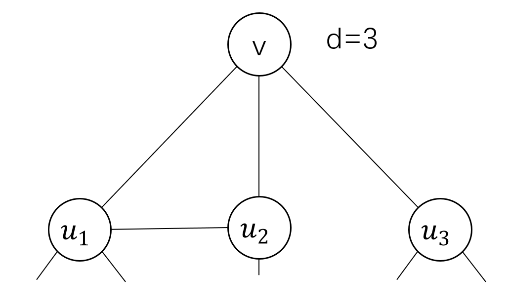
Figure 4: Degree-3 vertices in a triangle

Step 7 (Degree-3 vertices adjacent to some degree-4 vertex). If there is a degree-3 vertex $v$ adjacent to at least one degree-4 vertex, then branch on $u_{3}$ with Rule (B1) and in the branch of deleting $u_{3}$, we further branch on the dominating vertex $u_{1}$ with Rule (B2).

Vertex $u_{3}$ is a vertex of degree $\geq 3$ not dominating any neighbor of it. Thus each neighbor $w$ of $u_{3}$ is adjacent to at least one vertex out of $N[u_{3}]$ and then $|N(\{u_{3},w\})|\geq d(u_{3})$. Furthermore, vertex $v$ is adjacent to two vertices out of $N[u_{3}]$ and then $|N(\{u_{3},v\})|=d(u_{3})+1$. So we get a recurrence

$$T(k)\leq T(k-1)+T(k-d(u_{3})-1)+((d(u_{3}))-1)\times T(k-d(u_{3}))+1.$$

In the branch of deleting $u_{3}$, we further branch on the dominating vertex $u_{1}$ with Rule (B2). We get two branches

$${\tt aim}(G\setminus\{u_{1}\},k-1)\quad\mbox{and}\quad{\tt aim}(G\setminus N[\{u_{1},v\}],k-|N(\{u_{1},v\})|).$$

This leads to a recurrence

$$T(k)\leq T(k-1)+T(k-(d(u_{1})-1))+1.$$

The whole branches are

$$\begin{split}{\tt aim}(G\setminus\{u_{1},u_{3}\},k-2),\quad{\tt aim}(G\setminus N[\{u_{1},v\}],k-|N(\{u_{1},v\})|-1)&,\\ \mbox{and}\quad{\tt aim}(G\setminus N[\{u_{3},w\}],k-|N(\{u_{3},w\})|)\mbox{~{}for each $w\in N(u_{3})$}&.\end{split}$$

And the whole recurrence is

$$T(k)\leq T(k-2)+T(k-(d(u_{1})))+T(k-(d(u_{3})+1))+((d(u_{3}))-1)\times T(k-d(u_{3}))+1,$$

Table 1 shows the branching factors for different cases according to the value of $d(u_{1})$ and $d(u_{3})$. At least one vertex in $\{u_{1},u_{3}\}$ is a degree-4 vertex and we know the worst branching factor is 1.6957.

Table 1: The branching factors for different cases in Step 7

degree	branching factor
$d(u_{1})=4,d(u_{3})=4$	1.6445
$d(u_{1})=3,d(u_{3})=4$	1.6888
$d(u_{1})=4,d(u_{3})=3$	1.6957
$d(u_{1})=3,d(u_{3})=3$	-

The worst branching factors of the above seven steps are listed in Table 2. After Step 7, there are no degree-3 vertices adjacent to degree-4 vertices, and each connected component is either 3-regular or 4-regular.

Table 2: The branching factors of each of the first seven steps

Step	branching factor
Step 1	1.6181
Step 2	1.6181
Step 3	1.6717
Step 4	1.6957
Step 5	1.6595
Step 6	1.6581
Step 7	1.6957

Step 8 (3/4-regular graphs). Pick up an arbitrary vertex $v$ and branch on it with Rule (B1).

We do not need to analyze the branching factor of Step 8, since we will show that it will not exponentially affect the running time bound. Among all the branching factors in the first seven steps, the worst one is 1.6957, which is in Step 4 and Step 7. For a connected 3-regular graph, Step 8 can be applied for at most one time, as any properly induced subgraph of a connected 3-regular graph is neither a 3-regular nor a 4-regular graph. Thus, Step 8 will not affect the exponential part of the running time. We get that the algorithm runs in $O^{*}(1.6957^{k})$ time on any connected 3-regular graph. For a 3-regular graph $G$, since we can solve each connected component in $O^{*}(1.6957^{k})$ time and there are at most $n$ connected components, we can solve $G$ in $O^{*}(1.6957^{k})$ time. For a connected 4-regular graph, after executing Step 8 for once (which will not exponentially affect the running time), the algorithm can always branch with a branching factor at most 1.6957 or get a 3-regular graph. For the latter case, we solve it in $O^{*}(1.6957^{k})$ time directly by the above analysis. Thus, we can always solve a connected 4-regular graph in $O^{*}(1.6957^{k})$ time. By the similar argument, if each connected component is 3-regular or 4-regular, we can solve the graph in $O^{*}(1.6957^{k})$ time. This also implies that we can solve any graph in $O^{*}(1.6957^{k})$ time.

Theorem 4.1.

Almost Induced Matching can be solved in $O^{*}(1.6957^{k})$ time and polynomial space.

References

- [1] Abu-Khzam, F.N., Collins, R.L., Fellows, M.R., Langston, M.A., Suters, W.H., Symons, C.T.: Kernelization algorithms for the vertex cover problem: Theory and experiments. In: Arge, L., Italiano, G.F., Sedgewick, R. (eds.) Proceedings of the Sixth Workshop on Algorithm Engineering and Experiments and the First Workshop on Analytic Algorithmics and Combinatorics, New Orleans, LA, USA, January 10, 2004. pp. 62–69. SIAM (2004)
- [2] Cameron, K.: Induced matchings. Discrete Applied Mathematics 24(1-3), 97–102 (1989)
- [3] Chor, B., Fellows, M., Juedes, D.: Linear kernels in linear time, or how to save k colors in steps. In: International workshop on graph-theoretic concepts in computer science. pp. 257–269. Springer (2004)
- [4] Duckworth, W., Manlove, D.F., Zito, M.: On the approximability of the maximum induced matching problem. Journal of Discrete Algorithms 3(1), 79–91 (2005)
- [5] Golumbic, M.C., Laskar, R.C.: Irredundancy in circular arc graphs. Discrete Applied Mathematics 44(1-3), 79–89 (1993)
- [6] Golumbic, M.C., Lewenstein, M.: New results on induced matchings. Discrete Applied Mathematics 101(1-3), 157–165 (2000)
- [7] Gupta, S., Raman, V., Saurabh, S.: Maximum r-regular induced subgraph problem: Fast exponential algorithms and combinatorial bounds. SIAM Journal on Discrete Mathematics 26(4), 1758–1780 (2012)
- [8] Hoi, G., Sabili, A.F., Stephan, F.: An exact algorithm for finding maximum induced matching in subcubic graphs. arXiv preprint arXiv:2201.03220 (2022)
- [9] Kanj, I., Pelsmajer, M.J., Schaefer, M., Xia, G.: On the induced matching problem. Journal of Computer and System Sciences 77(6), 1058–1070 (2011)
- [10] Ko, C., Shepherd, F.B.: Bipartite domination and simultaneous matroid covers. SIAM Journal on Discrete Mathematics 16(4), 517–523 (2003)
- [11] Kobler, D., Rotics, U.: Finding maximum induced matchings in subclasses of claw-free and p 5-free graphs, and in graphs with matching and induced matching of equal maximum size. Algorithmica 37(4), 327–346 (2003)
- [12] Kratsch, D., Fomin, F.: Exact exponential algorithms. Springer-Verlag Berlin Heidelberg (2010)
- [13] Kumar, A., Kumar, M.: Deletion to induced matching. arXiv preprint arXiv:2008.09660 (2020)
- [14] Mathieson, L., Szeider, S.: Editing graphs to satisfy degree constraints: A parameterized approach. Journal of Computer and System Sciences 78(1), 179–191 (2012)
- [15] Moser, H., Sikdar, S.: The parameterized complexity of the induced matching problem. Discrete Applied Mathematics 157(4), 715–727 (2009)
- [16] Moser, H., Thilikos, D.M.: Parameterized complexity of finding regular induced subgraphs. Journal of Discrete Algorithms 7(2), 181–190 (2009)
- [17] Stockmeyer, L.J., Vazirani, V.V.: Np-completeness of some generalizations of the maximum matching problem. Information Processing Letters 15(1), 14–19 (1982)
- [18] Xiao, M., Kou, S.: Parameterized algorithms and kernels for almost induced matching. Theoretical Computer Science 846, 103–113 (2020)
- [19] Xiao, M., Tan, H.: Exact algorithms for maximum induced matching. Information and Computation 256, 196–211 (2017)