Superpixels algorithms through network community detection

Abstract

Community detection is a powerful tool from complex networks analysis that finds applications in various research areas. Roughtly speaking, it aims at grouping together nodes of a network that are densely connected while having few links with other groups. Several image segmentation methods rely for instance on community detection algorithms as a black box in order to compute undersegmentations [1, 2, 3, 4, 5, 6, 7, 8], i.e. a small number of regions that represent areas of interest of the image. However, to the best of our knowledge, the efficiency of such an approach w.r.t. superpixels, that aim at representing the image at a smaller level while preserving as much as possible original information, has been neglected so far. The only related work seems to be the one by Liu et al. [9] that developed a superpixels algorithm using a so-called modularity maximization approach, leading to relevant results. We note that the algorithm used is a variant of a well-known community detection algorithm that has however not been tested in a context other than image segmentation. We follow this line of research by studying the efficiency of superpixels computed by state-of-the-art community detection algorithms on a $4$-connected pixel graph, so-called pixel-grid. We first detect communities on such a graph and then apply a simple merging procedure that allows to obtain the desired number of superpixels. As we shall see, such methods result in the computation of relevant superpixels as emphasized by both qualitative and quantitative experiments, according to different widely-used metrics based on ground-truth comparison or on superpixels only. We observe that the choice of the community detection algorithm has a great impact on the number of communities and hence on the merging procedure. Similarly, small variations on the pixel-grid may provide different results from both qualitative and quantitative viewpoints. For the sake of completeness, we compare our results with those of several state-of-the-art superpixels algorithms as computed by Stutz et al. [10].

1 Introduction

In many real-life applications such as image segmentation or video analysis one may need to preprocess the image at hand in order to achieve great performances. One of the most natural such preprocessing is the computation of so-called superpixels or oversegmentations that represent the image at a smaller level while preserving as much as possible original information. Notable applications of superpixels include moving-object tracking, content-based image retrieval, biomedical imaging, indoor scene understanding, clothes parsing and convolutional neural networks. We refer the reader to recent comprehensive surveys for relevant references and more information on the topic [11, 12, 10]. We note that the literature mentions both the notion of superpixels and oversegmentation. According to Stutz et al. [10], the main difference lies in the possibility to control both the number of generated segments and their compactness, which leads to superpixels when present and to oversegmentation otherwise. As we shall see afterward community detection algorithms usually do not encompass an explicit way to control the number of segments but the merging procedure used does provide such a control. Moreover, the compactness can be adjusted by considering different graphs from the image. Hence the required characteristics for superpixels are fulfilled by this method: the segments form moreover a partition of the pixels, represent connected sets of pixels with great compactness and boundary adherence (see Stutz et al. [10]). As we shall discuss later, computing superpixels is not efficient at the moment due to the implementation choices made for the sake of reproduciblity.

Our contribution

We illustrate that the use of community detection algorithms on the most natural graph one can imagine, namely the pixel graph with $4$-connectivity (so-called pixel-grid, see Figure 1) yields superpixels that achieve state-of-the-art results w.r.t. several metrics [10], both objective and subjective (i.e. depending on ground-truth segmentations). We will also consider graphs with a given radius $r$, meaning that pixels are considered neighbors with all pixels at distance at most $r$. This work complements a previous analysis of Liu et al. [9] who used a variant of a well-known community detection algorithm on a similar graph to compute superpixels. We note here that such a variant has not been studied in a context other than image segmentation and that it seems to deeply rely on the particular structure of the pixel-grid. Our study compares three well-studied community detection algorithms on the same pixel-grid, namely Label Propagation [13], Louvain [14] and InfoMap [15]. We emphasize that using different community detection algorithms on the same graph may lead to great differences on the outputted superpixels, mainly from the qualitative viewpoint. For the sake of reproducibility, we rely on the evaluation of state-of-the-art methods proposed by Stutz et al. [10]. As noticed by the authors, superpixel algorithms are often compared to other approaches with undisclosed or default parameter settings and with variating implementation of metrics. In particular, Stutz et al. [10, Appendix D] provide a thorough parameter optimization analysis. All the experiments proposed in our work rigourously reproduce the work of Stutz et al. [10] for which both implementation and plot files are available free of charge. The results presented illustrate the relevance of this approach compared to many state-of-the-art algorithms using different principles.

Related work

There are a tremendous number of superpixels algorithm in the literature that rely on many different techniques. For instance, gradient-ascent and graph-based methods have been proposed for computing superpixels. In both cases some variations are possible but the main idea remains the same: starting with a primary grouping of pixels that is then refined until some convergence criterion is reached for the former; computing a graph based on pixels of the image for the latter (see [11]). We hereafter focus on graph-based methods due to their relevance with our work. In the last decades, many works took advantage of graph theoretic tools to compute segmentation algorithms. This is for instance the case of graph cuts which rely on flow algorithms on the pixel-grid to compute hard segmentations of images [16]. Another notable use of the pixel-grid is the work of Felzenszwalb and Huttenlocher [17] who used minimum spanning trees algorithms to compute efficient segmentations. More recently, community detection algorithms have been used in several works as a tool to compute undersegmentations [1, 2, 3, 4, 5, 6, 7, 8]. In most cases the used algorithm relies either on a large graph or on a presegmented graph augmented with some features. For the former method, let us mention the work of Nguyen et al. [7] who relied on the Louvain algorithm [14] on a pixel-grid of radius $20$ and on a merging procedure to obtain the sought segmentation. Regarding the latter approach, Mourchid et al. [6] first computed superpixels using Mean-Shift [18] as their initial segmentation and then used color and texture-based features to obtain their final segmentation through community detection algorithms. However, all aforementioned works aim at computing undersegmentations and thus do not evaluate intermediate results that may yield oversegmentations meeting many requirements of superpixels. Note that this phenomenon is actually noticed in the work of Nguyen et al. [7]. Very recently, Liu et al. [9] proposed a superpixels algorithm using a $8$-connected pixel-grid with radius $1$. The superpixels were detected using a greedy modularity maximization, a measure that quantifies the quality of a given community structure. Their algorithm heavily relies on the strong structural properties of pixel-grids and may thus not lead to relevant communities for other graphs. The final undersegmentation was also computed with a merging procedure.

Outline

We begin by giving a general picture of the approach with a particular focus on community detection algorithms (Section 2). We next turn our attention to experimental results, both qualitative (Section 4.2) and quantitative (Section 4.1). Before doing so, we thoroughly describe datasets (Section 3.1), metrics (Section 3.2) and methods (Section 3.3) used in our comparative studies. Finally, we give insights on the impact of the community detection algorithms used in Section 5 and conclude this work by some perspectives Section 6.

2 Description of the framework

Original image

Corresponding graph

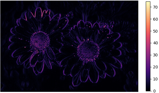
Graph enhancement

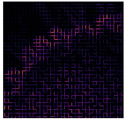
Merged image

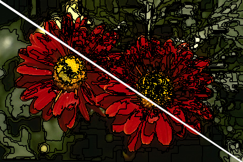
Figure 1: Different steps of the algorithm starting from an image from BSDS500. The lower part of the resulting image has $200$ superpixels while the upper part shows $1000$ regions.

Throughout the paper we consider $(n\times n)$-sized images with pixels $I=\{p_{1,1}\ldots,p_{n,n}\}$. As observed in previous works [8, 10], the L*a*b* space is the closest to the human perception and is hence the one chosen for our study.

Building the graph

A graph is a pair $G=(V,E)$ where $V$ denotes its vertex set and $E\subseteq[V]^{2}$ its edge set. Here $[V]^{2}$ denotes the set of all pairs of elements of $V$. Unless stated otherwise the considered graphs are simple (without self-loops nor multiedges), undirected and weighted, meaning that every graph $G=(V,E)$ comes together with a weight function $\omega:E\rightarrow\mathbb{R}^{+}$. We consider as weight function a similarity measure that will be described Eq. 1. We consider the simplest way to obtain a graph from an image, that is by considering pixels as neighbors using the $4$-connectivity model within a given distance. More precisely, given an integer $r\geqslant 1$, called radius, we define the $r$-pixel grid graph of image $I$ as the graph $G_{r}=(V_{r},E_{r})$ where $V_{r}=I$ and there is an edge $pp^{\prime}$ in $E_{r}$ if the corresponding pixels are both on the same row or the same column of $I$ and at distance at most $r$ from each other. (Obviously edges with out-of-bounds indices are not considered in this process.) Note that the $1$-pixel grid is simply the graph obtained from the direct $4$-connected neighborhood of every pixel. In this work we will consider values of $r$ ranging from $1$ to $10$, the best results being achieved for $r=5$ in most cases. For the sake of comparison, Nguyen et al. [7] used a $20$-pixel grid to compute their undersegmentation, which implies that the used graph was significantly larger. Moreover, they removed edges whose similarity was below some fixed threshold $\rho$ but considered unweighted graphs. In our setting, we remove edges in a similar manner but we weight the remaining edges accordingly. We use a similarity measure based on the channel differences between pixels (or the mean of a region for a presegmented image), that is a Gaussian type radius basis function:

$$\omega(p,p^{\prime})=\exp{\frac{-|p-p^{\prime}|^{2}}{2\cdot\sigma^{2}}}$$ (1)

where $\sigma$ is a parameter that defines how close two regions must be for the corresponding edge weight to be significant. There are actually several graphs considered in the literature, some preserving all edges in a given radius (which corresponds to a threshold $\rho=0$) while other approaches preserve edges above a given threshold only. Moreover, some authors consider weighted graphs [9] while others use weight as a binary mask to remove or preserve unweighted edges [7]. As we shall see Table 1 and Section 5 these choices may have a great impact on pixel-grids and on computed communities.

Computing communities

The next step for computing superpixels is to detect communities on the given $r$-pixel grid. Roughly speaking, a community structure of a given graph is a partition of its vertex set such that every part is densely connected while there are few edges between two distinct parts. One may think of communities in social networks as a way to gather individuals that are similar according to some properties. Regarding image analysis, the intuition is that pixels that are similar (e.g. regarding some color features) should be contained in the same community. There exist many community detection algorithms that sometimes exhibit different behaviors and that may hence encompass different properties of the graph [19]. Our study will use three algorithms for the sake of comparison, that we briefly describe hereafter.

• Label Propagation [13] is an iterative algorithm that assigns labels to vertices, corresponding to communities. The initial step of the algorithm labels every vertex $\{v_{1},\ldots,v_{n}\}$ of an $n$-vertex graph with its corresponding index $1\leqslant i\leqslant n$. Labels are then propagated by considering vertices in a random order and giving to each vertex the majority label of its neighbors. The process stops when all vertices are labeled with the majority label of their respective neighborhoods. A particular feature of this algorithm is that two consecutive runs may end up with rather different community structures.

• Louvain [14] is an agglomerative algorithm that greedily optimizes the so-called modularity of the graph, a measure that qualifies a given community structure. Roughly speaking, the algorithm starts from an existing partition into communities (e.g. the singleton partition) and computes the gain obtained by moving any vertex to a different community. It stops when no valuable move remains and then merges each community into a single vertex, repeating this process until no valuable move is made.

• InfoMap relies on a flow-based and information theoretic method called the map equation [15]. Quoting the work of Rosvall et al. [20]:

  The map equation specifies the theoretical limit of how concisely we can describe the trajectory of a given walker in the network. With such a random walker as a proxy for real flow, minimizing the map equation over all possible network partitions reveals important aspects of network structure with respect to the dynamics of the network.

  Rosvall et al. [20] moreover emphasize that methods based on the map equation and on modularity maximization may yield really different community structures, making the study of those algorithms well-suited for our purpose.

$r=1$

$r=2$

$r=5$

$r=10$

aaaiImage

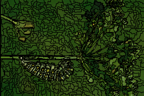
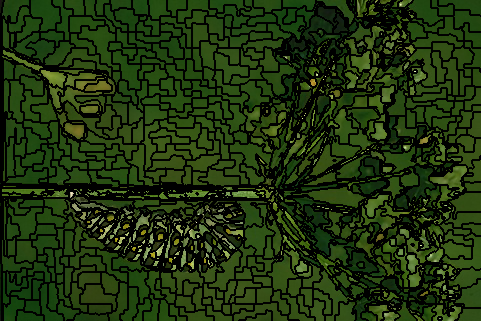
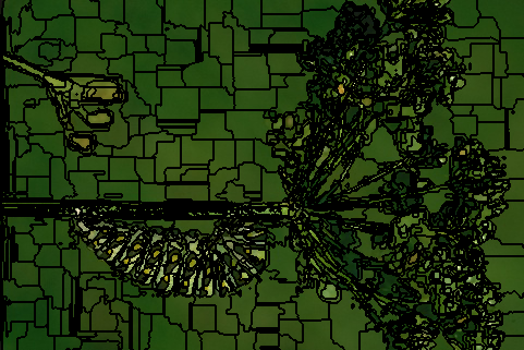
Figure 2: Impact of the radius for a sample image from BSDS500. Larger radius implies larger superpixels on background areas with more small regions around objects and shapes. All images are computed with a threshold $\rho=0.98$ and $K=1000$.

Merging communities

The final step of the procedure is to reduce further the number of superpixels produced by the algorithms. A similar procedure was used in several works [7, 9] to produce image segmentation based on both the size and the similarity of superpixels. As noticed for instance by Liu et al. [9], the sought number of superpixels $K$ can be explicitely managed by merging all communities with size smaller than $\frac{(n^{2})}{K}$. Note that there are many criteria that can be considered for merging initial oversegmentations, such as the size of regions and the similarity between regions. We choose in this work to focus on a merging procedure based on the sizes of the communities, namely by merging any small enough region with its closest neighboring one w.r.t. similarity defined Eq. 1 until the number of desired superpixels is reached. To that aim, we compute a Region Adjacency Graph with radius $1$. We note that in order to avoid too many very small superpixels, w e begin by merging communities the size of which is less than $\frac{n^{2}}{10\cdot K}$. Obviously, this approach allows to control the number of outputted regions, thus meeting the requirements of a superpixels algorithm. See Figure 1 for an example of the framework. Let us mention here that Liu et al. [9] chose a different approach in their work by merging small regions with the largest neighboring one.

Details of implementation

We conducted all experiments using python3 with scikit-image for dealing with images, networkx and networkit for most graph-related operations and the module Infomap. Moreover, metrics are replicated from the C++ implementation of Stutz et al. [10]. Source code is available on a public github repository. As mentioned in the introductory section, the aim of this study is to enlight the relevance of community detection to compute superpixels. We hence did not aim at achieving great performance in computing the segmentations. We will discuss this matter more thoroughly Section 6.

3 Experimental setup

3.1 Datasets

We now give a brief description of the datasets used in our experiments as well as references and links to retrieve the raw datasets. Let us recall that we closely follow the work of Stutz et al. [10, Section 4] and use datasets that have been preprocessed. Most of the following paragraphs are extracted from [10].

BSDS500 [21]

The Berkeley Segmentation Dataset 500 is one of the earliest that has been used for superpixel algorithm evaluation. It contains $500$ images that come together with a set of at least $5$ ground truth for every image. We consider the $200$ images that are part of the test set. Following the work of Stutz et al. [10] we choose for each image the ground truth providing the worst score for a given metric and average such values over all images.

SBD [22]

The Stanford Background dataset combines $715$ images from several datasets implying that the sizes, qualities and scenes are varying between images. The scenes tend to be more complex than those of the BSDS500 dataset. The used dataset provided by Stutz et al. [10] has been preprocessed to ensure connected segments in ground truth and contains $477$ randomly chosen images.

NYUV2 [23]

The NYU Depth Dataset V2 contains $1449$ images. The labels provided by Silberman et al. [23] ensure connected segments and the data has been further preprocessed by Stutz et al. [10] (following Ren and Bo [24]) to remove small unlabeled regions. Note that the provided ground truth is of lower quality than in the BSDS500 dataset. The preprocessed dataset contains $399$ randomly chosen images.

SUNRGBD [25]

The Sun RGB-D dataset is made of $10335$ images combined from several datasets [26, 27], including NYUV2 (which has here been excluded). Images have been acquired through several devices [25] and ground truth has been preprocessed by Stutz et al. [10] in a similar manner than for NYUV2. The preprocessed dataset contains $400$ images chosen at random.

Pixel-grids

Table 1 provides some information about the pixel-grid obtained for different radii and threshold values on the BSDS500 dataset. We use $G_{r}^{\rho}$ to denote a $r$-pixel grid where only edges with a weight greater than $\rho$ are preserved. Note that due to the threshold some vertices may become isolated and are thus not added to the graph. We also illustrate Figure 2 the impact the radius has on computed superpixels. We will discuss further these differences Section 4.

	vertices	edges	weight	CO (Table 2)
$G_{1}^{0}$	$154401$	$308000$	$254752$	$0.31892$
$G_{1}^{0.98}$	$97808$	$117528$	$116846$	$0.19405$
$G_{2}^{0}$	$154401$	$615198$	$480182$	$0.39695$
$G_{2}^{0.98}$	$103765$	$199446$	$198228$	$0.18930$
$G_{5}^{0}$	$154401$	$1531980$	$1079130$	$0.50955$
$G_{5}^{0.98}$	$110143$	$377524$	$375030$	$0.17446$

Table 1: Number of vertices, edges and total edge weight for $r$-pixel grids with $r$ in in $\{1,2,5\}$ and $\rho$ in $\{0,0.98\}$. Values are rounded. Last column indicates the compactness for $1000$ superpixels on BSDS500.

Finally, the last column gives the Compactness (see Section 3.2) on the BSDS500 dataset for $K=1000$ superpixels. As one can observe, the best values are achieved for a radius $r=2$ and a small threshold. This property actually holds regardless of the number of sought superpixels and thus allows to control the compactness of the superpixels. However, all other metrics presented Table 2 have worse values for such combinations of radius and threshold. We hence choose not to include them in the remainder of our study. Nonetheless, let us mention that Stutz et al. [10, Fig. 8] provides Compactness values for all considered datasets. For $1000$ superpixels, the best value is achieved by TPS with $0.56146$ while SEEDS and ETPS are the two lowest with $0.08952$ and $0.16260$, respectively. This enlightens that results provided by InfoMap are also relevant w.r.t. Compactness.

Metric	Notations
Ground truth-based
$\text{Rec}(\mathcal{G},\mathcal{S})=\frac{TP(\mathcal{G},\mathcal{S})}{TP(\mathcal{G},\mathcal{S})+FN(\mathcal{G},\mathcal{S})}$	$FN(\mathcal{G},\mathcal{S})$: number of false negative boundary pixels in $\mathcal{S}$ w.r.t. $\mathcal{G}$
	$TP(\mathcal{G},\mathcal{S})$: number of true positive boundary pixels in $\mathcal{S}$ w.r.t. $\mathcal{G}$
$\text{UE}(\mathcal{G},\mathcal{S})=\frac{1}{\left|I\right|}\cdot\sum_{G_{i}}\sum_{S_{j}\cap G_{i}\neq\emptyset}\min{\{\left|S_{j}\cap G_{i}\right|,\left|S_{j}\setminus G_{i}\right|\}}$
No ground truth
$\text{EV}(\mathcal{S})=\frac{\sum_{S_{j}}\left|S_{j}\right|\cdot(\mu(S_{j})-\mu(I))^{2}}{\sum_{1\leqslant i\leqslant j\leqslant n}(I(p_{i,j})-\mu(I))^{2}}$	$\mu(\cdot)$: mean color of its argument
$\text{CO}(\mathcal{S})=\frac{1}{\left|I\right|}\cdot\sum_{S_{j}}\left|S_{j}\right|\cdot\frac{4\Pi\cdot A(S_{j})}{P(S_{j})}$	$A(S_{j})$: area of superpixel $S_{j}$
	$P(S_{j})$: perimeter of superpixels $S_{j}$

Table 2: Presentation of the metrics considered in this work together with needed notations.

3.2 Evaluation metrics

There are many metrics that can be used to assess the quality of superpixels algorithms, mostly relying on a ground truth segmentation of the image at hand. In this work we choose four metrics that have been introduced in various articles [28, 29, 30, 31]. Our choice is here again guided by Stutz et al. [10, Section 5] who give a detailed analysis of many metrics and ultimately focus on these ones. In the remaining of this section and in a slight abuse of notation we let $I(p_{i,j})$, $1\leqslant i\leqslant j\leqslant n$ denote the intensity of pixel $p_{i,j}$.   We moreover let $\mathcal{S}=\{S_{1},\ldots,S_{p}\}$ and $\mathcal{G}=\{G_{1},\ldots,G_{t}\}$ be partitions of a same image $I$ into superpixels and ground truth segmentation, respectively. All metrics are summarized Table 2. We give hereafter a brief overview of such metrics as presented by Stutz et al. [10].

Boundary recall (Rec) is widely used to assess the quality of a superpixel segmentation, and more precisely boundary adherence given ground truth. Under-segmentation error (UE) aims at measuring the overlap of superpixels with multiple, nearby ground truth segments. We note that the original formulation for Under-Segmentation Error was given by Levinshtein et al. [32] as follows:

$$\text{UE}_{Levin}(\mathcal{G},\mathcal{S})=\frac{1}{\left|\mathcal{G}\right|}\cdot\sum_{G_{i}}\frac{\big{(}\sum_{S_{j}\cap G_{i}\neq\emptyset}\left|S_{j}\right|\big{)}-\left|G_{i}\right|}{\left|G_{i}\right|}$$

However, as observed for instance in [33, 28] such a definition penalizes superpixels overlapping only slightly with neighboring ground truth segments and is not constrained to lie in $[0,1]$.  The adapted version chosen by Stutz et al. [10] has been proposed by Neubert and Protzel [28]. Explained variation (EV) [31] quantifies the quality of a superpixel segmentation by assessing boundary adherence without relying on human annotations. High EV scores means better superpixels explanation of the variation of the image. Compactness (CO) has been introduced by Schick et al. [30] to evaluate the compactness of superpixels. Compactness compares the area of a superpixel $S_{j}$ with the area of a circle with the same perimeter $P(S_{j})$. High CO value means better compactness.

3.3 Methods for comparison

We now briefly describe the state-of-the art methods used in our experiments. We based our choices on the work of Stutz et al. [10] which highlighted the efficiency of chosen methods w.r.t. metrics defined Section 3.2. In order to present a comparative study as meaningful as possible, we selected a couple of the best methods for different superpixels paradigms, namely density, graph, path, clustering and energy optimization based methods. The presentation of such methods is inspired by [10, Section 3].

Density-based

Such algorithms perform mode-seeking in a computed density image and usually do not offer control on the number of superpixels or their compactness [10]. Yet tuning the parameters can allow to achieve such objectives. We compare the presented method to EAMS [18] and QS [34].

Graph-based

The common feature of these methods is to extract a graph from the image at hand and then to use graph-theoretic tools to compute superpixels. Many tools have been used, such as network flows (graph cuts [16]) and minimum spanning trees [17]. Hence the main difference lies in the method used to compute the superpixels, the graph usually being based on a pixel (dis)similarity measure. We compare the presented method to FH [17] and ERS [29].

Path-based

Methods based on path detection compute superpixels by creating paths between seeds respecting some criteria. We compare the presented method to the TPS [35] algorithm, which relies on edge detection.

Clustering-based

These algorithms are inspired by clustering methods such as $k$-means and are close to the approach we consider here. Like for path-based methods, clustering-based superpixels algorithms use seeds and several image-related information as features to group pixels together. As noted in Stutz et al. [10], the resulting superpixels may be disconnected and further postprocessing is needed to ensure connectivity. We compare the presented method to SLIC [33].

Energy optimization-based

Starting from a regular grid, pixels are then exchanged with neighborhing superpixels w.r.t. some energy function. These methods achieve high accuracy and efficiency. We compare the presented method to SEEDS [36] and ETPS [37].

4 Experimental results

We focus in this section on superpixels obtained using InfoMap, which provides the best trade-off w.r.t. the quality of both qualitative and quantitative comparisons. We will see Section 5 that using different community detection algorithms such as Label Propagation or Louvain may lead to a bit worse quantitative results with a significant qualitative difference. Moreover, one advantage of such an algorithm compared to Label Propagation or Louvain is that it gives consistent community structures from one image to another, allowing a better control on the number of superpixels in the merging procedure.

Parameters

Besides the parameters specific to the chosen community detection algorithms this approach does not require a lot of parameter tuning. More precisely, one needs to fix values for the radius of the pixel-grid $r$, the threshold $\rho$ relative to Eq. 1 to decide which edges to preserve, the number of desired superpixels and the parameter $\alpha$ in Eq. 1. The latter has been experimentally chosen as $\alpha=125$. We recall Table 1 for the size of the pixel-grid according to both radius and threshold values. Our experiments show that choosing a combination of $r=5$ and $\rho=0.98$ provides relevant superpixels while maintaining a graph of reasonable size. We will present Section 5 some results using different radii and observe that their performances are a bit worse. Similarly, metrics computed with smaller threshold values were almost always significantly worse and are thus not reported here, with the notable exception of Compactness which can be improved using smaller values for $\rho$ (the better being $0$, meaning not filtering the pixel-grid, recall Table 1). Regarding the merging procedure the only parameter needed is the desired number of superpixels, which will vary from $200$ to $5000$ with different increasing steps: $200$ up to $1000$ and $500$ up to $2500$. We also compute $5000$ superpixels.

4.1 Quantitative comparison

We first turn our attention to quantitative comparison with methods mentioned Section 3.3 on datasets described Section 3.1. We compare our results with results extracted from the work of Stutz et al. [10]. Recall that we compute the metrics on superpixels generated using InfoMap on a $5$-pixel grid and with $\rho=0.98$ as threshold for all datasets, which provide the most relevant results. However, we will see Figure 5 that small variations of the radius may have an impact on the computed metrics.

Figure 3: Quantitative comparison on datasets described Section 3.1. Values for other methods are reported from Stutz et al. [10]. The results presented for this framework use a threshold value $\rho=0.98$ and a radius $r=5$.

As one can see Figure 3, this approach produces relevant results for all metrics. The recall values lie in the top three methods in any dataset. A similar observation holds for UE values while the best EV is achieved for a large number of superpixels. We also display standard deviation on metrics for all datasets. For the sake of readability, we do not display standard deviations for state-of-the-art methods. Such values can be found in [10, Fig. 9] and indicate that SEEDS and ETPS tend to have smaller standard deviations than InfoMap for Rec. On the other hand, the displayed values for UE and EV are rather similar than the ones in [10, Fig. 9]. We note that for the SBD dataset the mean number of superpixels when $K=5000$ is actually $4984$. This comes from the fact that for a few images, InfoMap computed a small number of communities and thus the method does not produce the exact number of superpixels. This is the case for exactly five images, and the number of superpixels produced for three of them is less than $4000$.

4.2 Qualitative comparison

aaaiImage

BSDS500

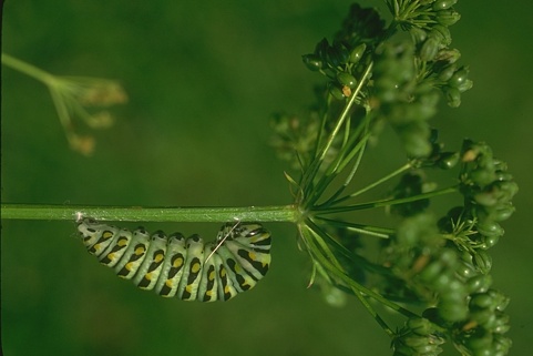
SBD

NYUV2

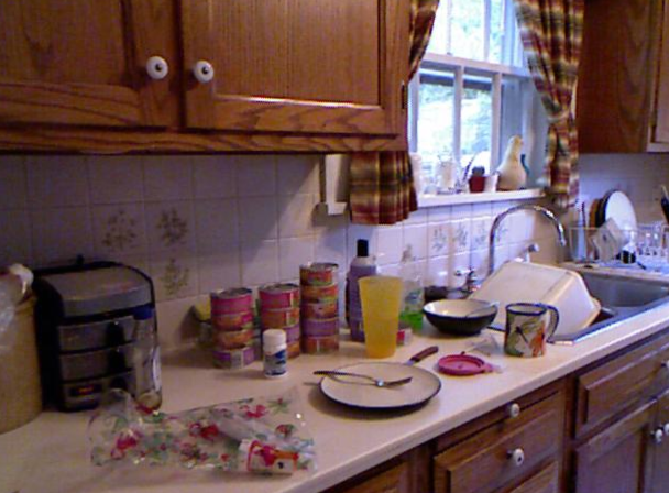
SUNRGBD

aaaiSEEDS

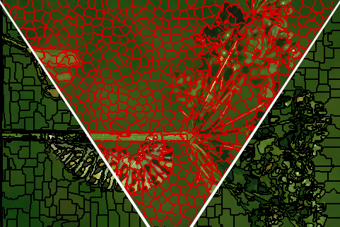
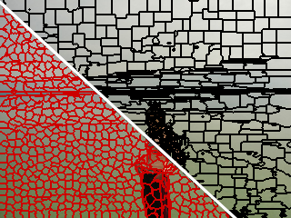
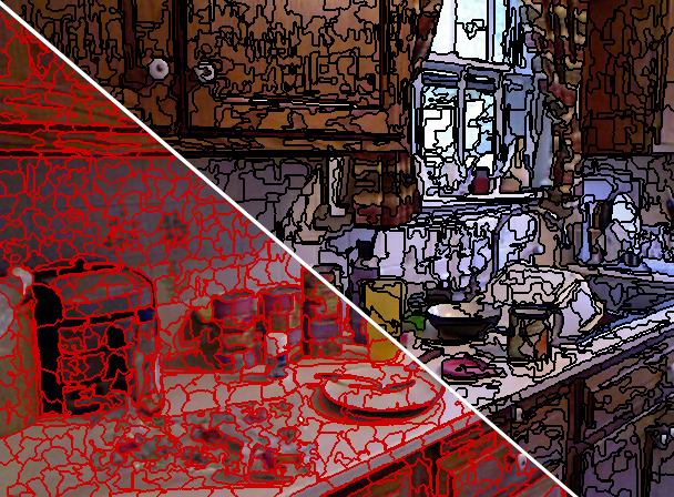
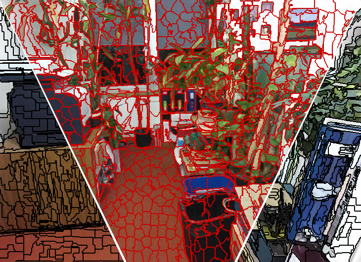
aaaiETPS

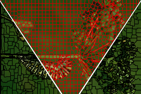
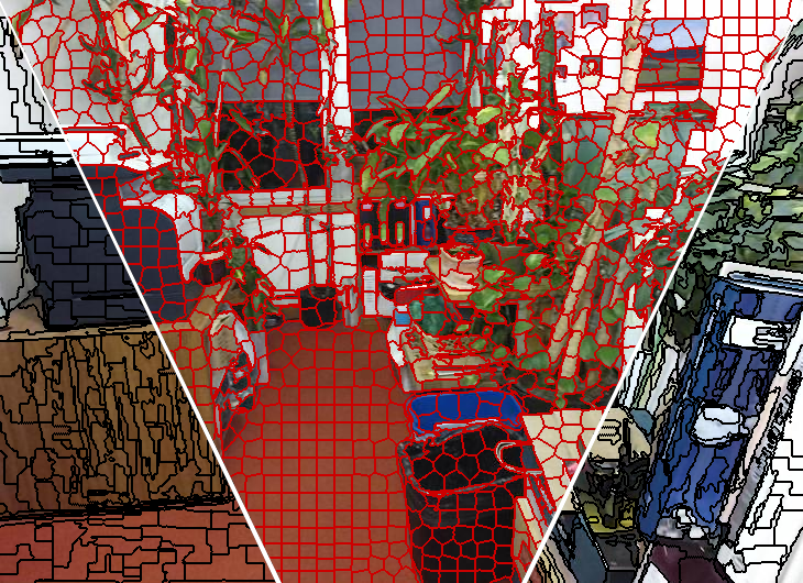
aaaiSLIC

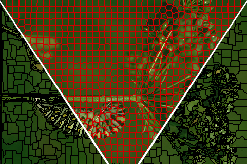
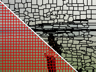
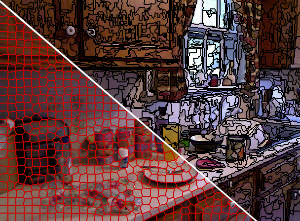
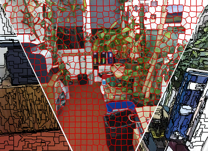
Figure 4: Qualitative comparison with selected methods, namely SEEDS, SLIC and ETPS on selected datasets with a number of superpixels of $K=1000$.

We now give some examples from datasets that illustrate the superpixels achieved by this method compared to some approaches described Section 3.3. Figure 4 emphasizes that the computed superpixels exhibit regularity and compactness on background areas and are less regular around objects. They show some similarities with superpixels computed by SEEDS and ETPS, methods that present the best result w.r.t. chosen metrics as seen Section 4.1. On the other hand, their regularity and compactness is not as clearly defined as SLIC. Note however that as shown Table 1 and Figure 2 the above properties can be adjusted by using different radius and threshold values. Hence, depending on the image at hand a simple adjustment of these values may lead to significant differences between superpixels.

5 The impact of community detection

In this section we discuss the impact the choice of the community detection algorithm may have on the computed superpixels. We limit our study to the BSDS500 dataset which provides meaningful insights. We begin by showing Table 3 the number of communities computed by each algorithm for radii $r\in\{2,5\}$ and threshold $\rho\in\{0,0.98\}$ used for building the pixel-grid. The difference in the number of computed communities along with their sizes emphasizes a difference in the regularity and the sizes of said communities. This has a great impact on the merging procedure that provides the final superpixels.

$G_{2}^{0}$	Communities		Max. size		Min. size
	$mean$	($std$)	$mean$	($std$)	$mean$	($std$)
LP	$5760$	($3228$)	$2579$	($1231$)	$1.2$	($0.39$)
Louvain	$79$	($29$)	$5840$	($1653$)	$97$	($234$)
InfoMap	$2780$	($634$)	$206$	($25$)	$2$	($0.34$)

$G_{2}^{0.98}$	#Communities		Max. size		Min. size
	$mean$	($std$)	$mean$	($std$)	$mean$	($std$)
LP	$72359$	($23599$)	$726$	($635$)	$1$	($0$)
Louvain	$63230$	($25616$)	$2126$	($1266$)	$1$	($0$)
InfoMap	$65374$	($24873$)	$133$	($36$)	$1$	($0$)

$G_{5}^{0}$	#Communities		Max. size		Min. size
	$mean$	($std$)	$mean$	($std$)	$mean$	($std$)
LP	$1924$	($1308$)	$10940$	($6120$)	$1.79$	($0.41$)
Louvain	$46$	($19$)	$10759$	($3786$)	$180$	($563$)
InfoMap	$1054$	($335$)	$684$	($93$)	$2.06$	($0.31$)

$G_{5}^{0.98}$	#Communities		Max. size		Min. size
	$mean$	($std$)	$mean$	($std$)	$mean$	($std$)
LP	$63909$	($23472$)	$2053$	($1890$)	$1$	($0$)
Louvain	$54998$	($24671$)	$3490$	($2194$)	$1$	($0$)
InfoMap	$57176$	($24175$)	$371$	($115$)	$1$	($0$)

Table 3: Statistics of the communities computed by algorithms on the BSDS500 dataset. The number of communities as well as the maximum and minimum sizes are reported. For all values we show mean and standard deviation.

Quantitative difference between algorithms

Figure 5: Quantitative comparison between Label Propagation, Louvain and InfoMap on the BSDS500 dataset. The results presented use a threshold value of $0.98$ and are shown with radii $\{1,2,5,10\}$.

As one may observe Figure 5, considered methods provide relevant results with respect to chosen metrics. While all methods result in significant outcomes, InfoMap outperforms other considered algorithms. To emphasize the impact the radius may have on each algorithm, we choose $K=1000$ as the number of computed superpixels. The difference observed on metrics is actually similar for all values of superpixels and across datasets. An interesting observation is that using a $10$-pixel grid improves both Rec and EV but not UE while increasing the size of the graph. Even if performance is not taken into account in this study, we note that increasing the radius may slow down the computation of communities and hence does not seem to be well-suited for this framework. As mentioned previously, the set of communities computed by each algorithm shows significant variations that may explain the difference in computed metrics. This is also emphasized by a qualitative comparison of each algorithm.

Qualitative difference between algorithms

Figure 6 shows that InfoMap tends to exhibit more compact and regular superpixels. In particular, on images with a clearly identified background both Label Propagation and Louvain tend to group the background into a few large superpixels. This is mainly due to the ability of InfoMap to produce smaller communities (recall Table 3), which hence results in a regular initial oversegmentation for which the merging procedure yields relevant results.

aaaiLouvain

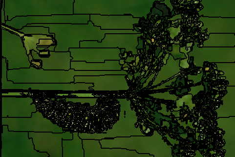
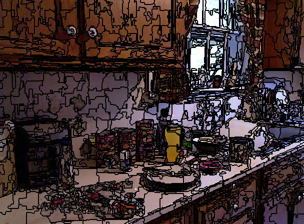
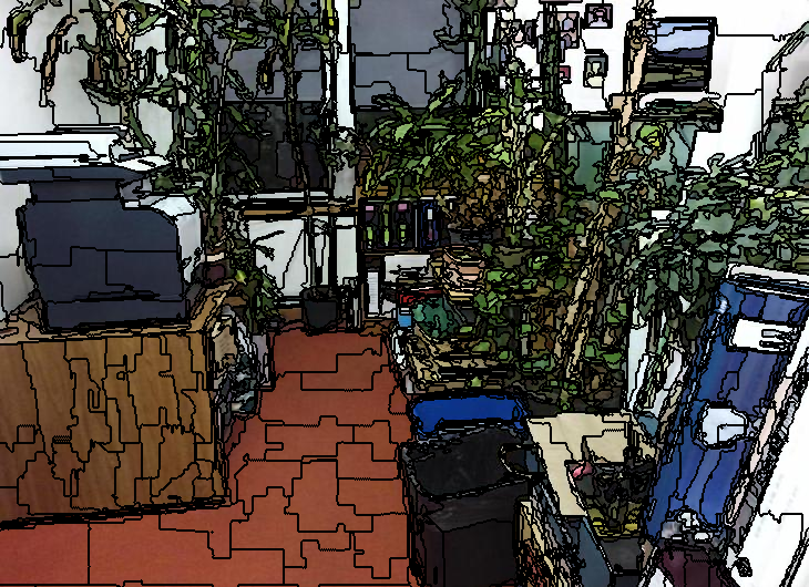
aaaiInfoMap

aaai$K=2500$

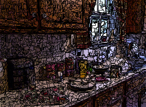
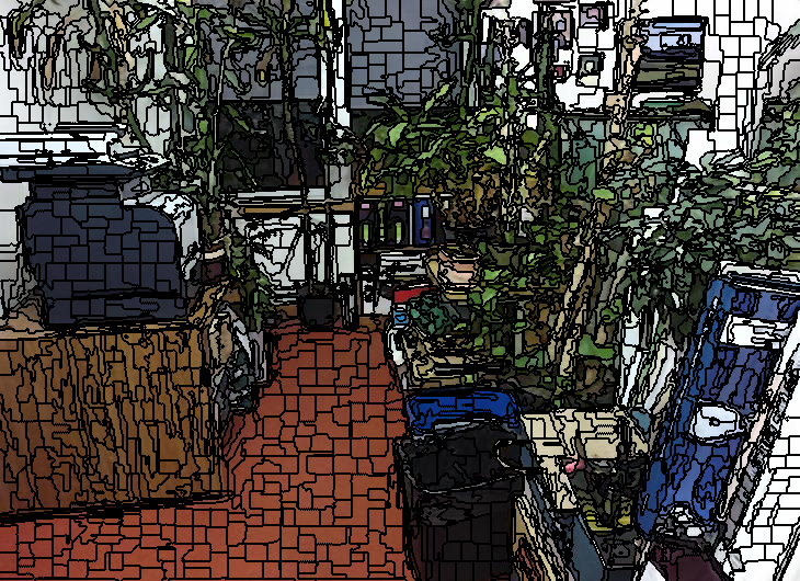
aaaiLP

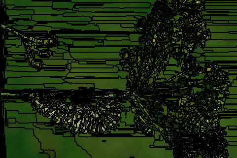
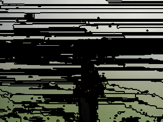
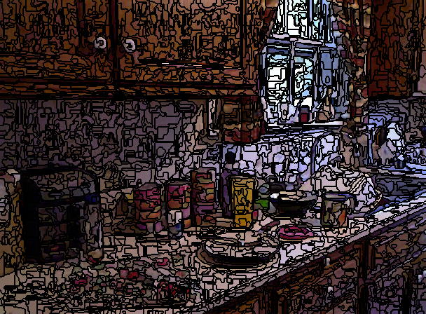
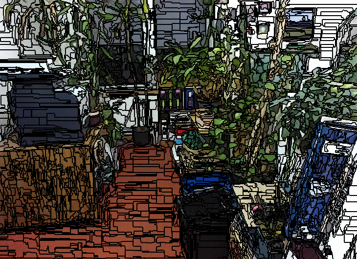
aaaiLouvain

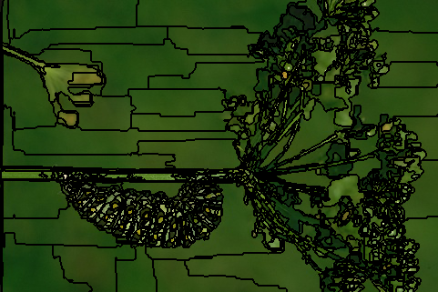
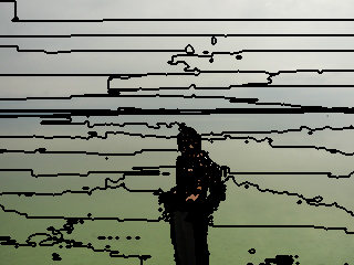
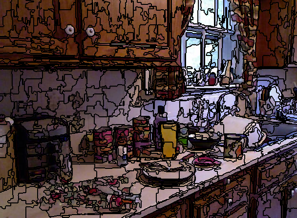
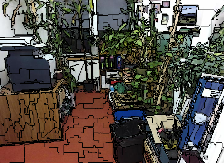
aaaiInfoMap

aaai$K=1000$

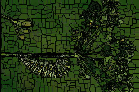
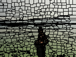
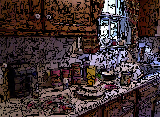
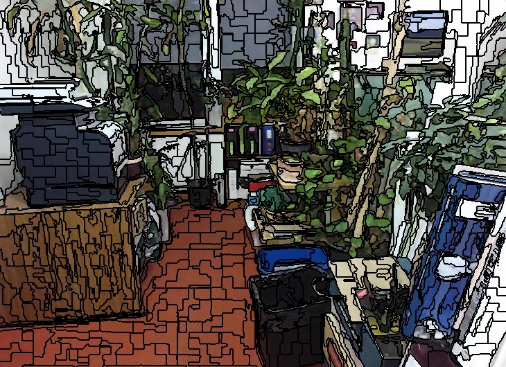
aaaiLP

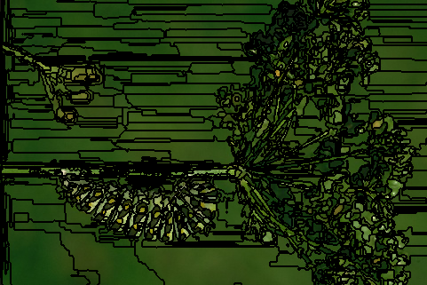
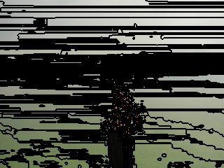
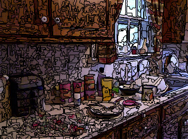
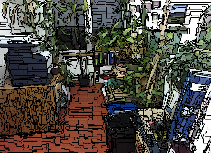
aaaiLouvain

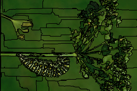
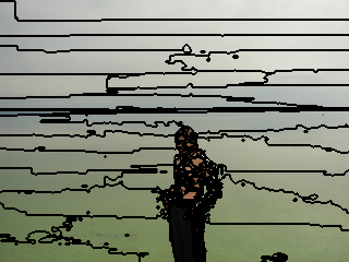
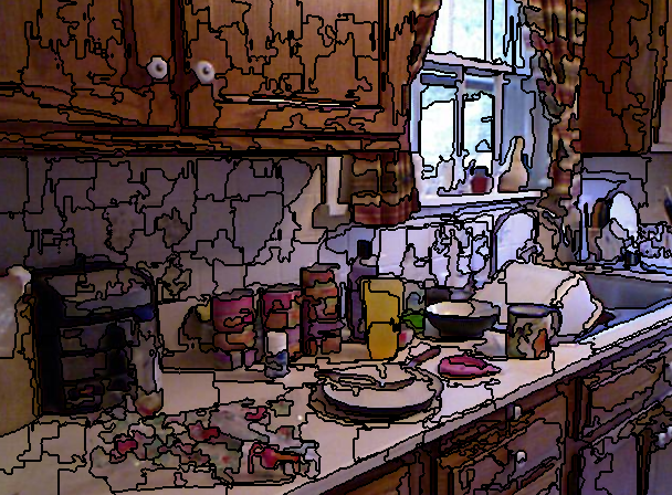
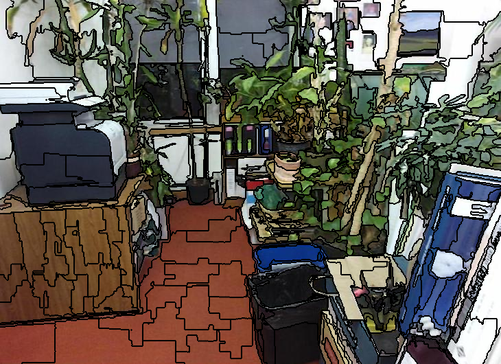
aaaiInfoMap

aaai$K=400$

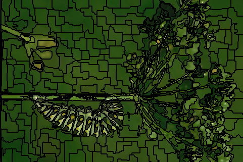
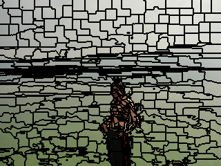
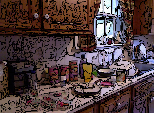
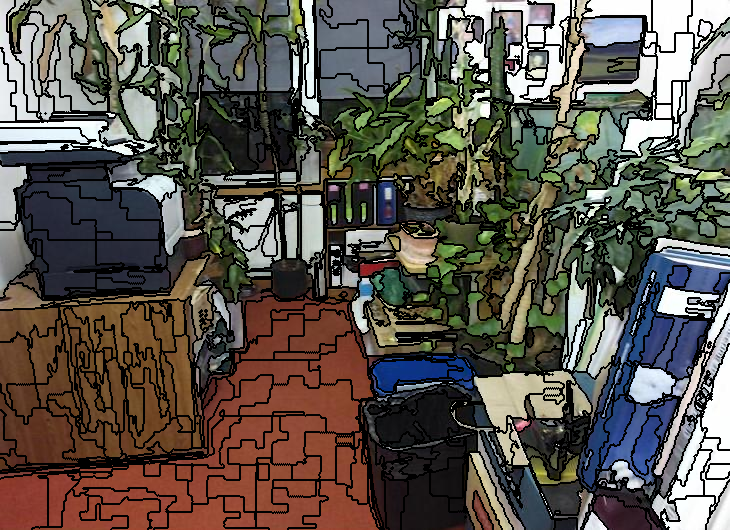
aaaiLP

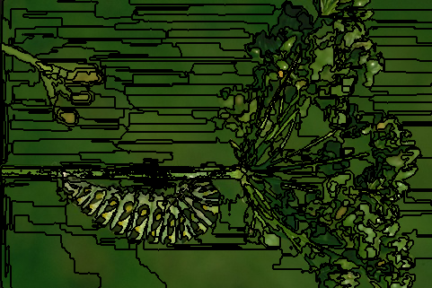
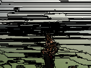
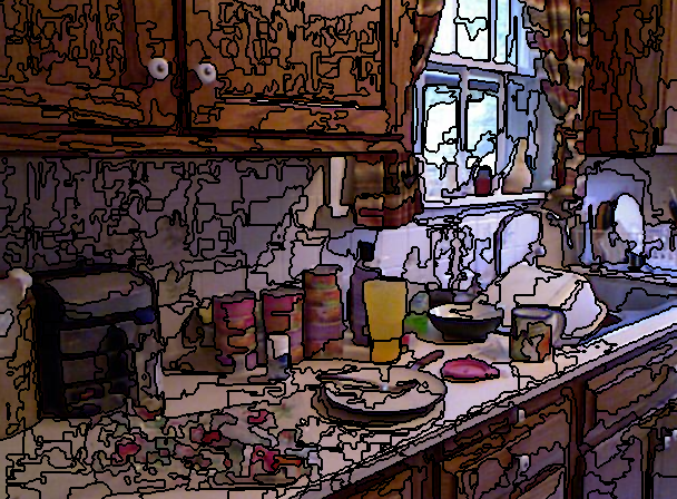
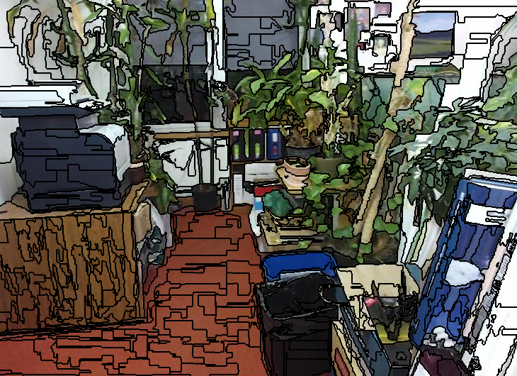
Figure 6: Qualitative comparison of outputted superpixels for selected datasets and community detection algorithms.

6 Conclusion

In this work we analyzed the relevance of superpixels computed through community detection algorithms and a merging procedure on a simple graph extracted from the image at hand. As mentioned Section 1 this approach has previously been used to compute undersegmentation in several works [1, 2, 3, 4, 5, 6, 7, 8] but, to the best of our knowledge, its use for the computation of superpixels has been neglected so far, the work of Liu et al. [9] being the only notable exception. We hence enlight the relevance of this approach by providing both qualitative and quantitative results w.r.t. state-of-the-art methods. One interesting property of this approach is its ability to evolve in time: novel community detection algorithms are frequently introduced (see e.g. [38]) and any improvement may also improve this approach. Notice that in this work we chose to rely on three well-studied and widely used algorithms to ensure the relevance of presented results. Hence as one of the most straightforward extension one may consider the analysis of more recent community detection algorithms in order to better understand the impact of such a choice. In particular it would be interesting to use a community detection algorithm that allows control on the number of computed communities. Another approach is to consider the graph extracted from the image. We here made the choice to work on a very simple graph, in particular using a weight function that only relies on color similarities. It would be interesting to study the impact of a more intricate similarity measure, for instance accounting for the histogram of oriented gradients as in [7] or with a trade-off between feature similarity and Euclidean distance as in [39]. We would like to mention that we also conducted experiments without weighting the graph, resulting in less relevant results. This seems to indicate that choosing a different weight function may have some impact on the results. Finally, the choices made for the merging procedure may result in different outcomes. We studied a basic strategy that provide relevant results, and it could be interesting to study further the impact of such a procedure. We note here that we tried another approach that merged really small regions first and then neighboring remaining regions if their similarity is above the similarity threshold $\rho=0.98$. Quite expectedly, this approach provided similar results and does not seem to lead to any improvement.

Acknowledgments

The author is deeply grateful to David Stutz for fruitful discussion and for pointing out the availability of the LaTeX source for the paper Superpixels: An evaluation of the state-of-the-art [10].

References

- [1] A. A. Abin, F. Mahdisoltani, H. Beigy, Wisecode: wise image segmentation based on community detection, The Imaging Science Journal 62 (6) (2014) 327–336.
- [2] O. A. Linares, G. M. Botelho, F. A. Rodrigues, J. B. Neto, Segmentation of large images based on super-pixels and community detection in graphs, IET Image Processing 11 (12) (2017) 1219–1228.
- [3] H. Hu, Y. van Gennip, B. Hunter, A. L. Bertozzi, M. A. Porter, Multislice modularity optimization in community detection and image segmentation, in: 2012 IEEE 12th International Conference on Data Mining Workshops, IEEE, 2012, pp. 934–936.
- [4] S. V. Belim, S. B. Larionov, An algorithm of image segmentation based on community detection in graphs, Computer Optics 40 (6) (2016) 904–910.
- [5] A. Browet, P. A. Absil, P. Van Dooren, Community detection for hierarchical image segmentation, in: Combinatorial Image Analysis: 14th International Workshop, IWCIA 2011, Madrid, Spain, May 23-25, 2011. Proceedings 14, Springer, 2011, pp. 358–371.
- [6] Y. Mourchid, M. El Hassouni, H. Cherifi, A general framework for complex network-based image segmentation, Multimedia Tools and Applications 78 (2019) 20191–20216.
- [7] T.-K. Nguyen, J.-L. Guillaume, M. Coustaty, An enhanced louvain based image segmentation approach using color properties and histogram of oriented gradients, in: Computer Vision, Imaging and Computer Graphics Theory and Applications: 14th International Joint Conference, VISIGRAPP 2019, Prague, Czech Republic, February 25–27, 2019, Revised Selected Papers 14, Springer, 2020, pp. 543–565.
- [8] S. Li, D. O. Wu, Modularity-based image segmentation, IEEE Transactions on Circuits and Systems for Video Technology 25 (4) (2014) 570–581.
- [9] T. Liu, F. Dai, W. Guo, F. Zhao, J. Wang, X. Wang, Superpixel segmentation algorithm based on local network modularity increment, IET Image Processing 16 (7) (2022) 1822–1830.
- [10] D. Stutz, A. Hermans, B. Leibe, Superpixels: An evaluation of the state-of-the-art, Computer Vision and Image Understanding 166 (2018) 1–27.
- [11] A. Ibrahim, E.-S. M. El-kenawy, Image segmentation methods based on superpixel techniques: A survey, Journal of Computer Science and Information Systems 15 (3) (2020) 1–11.
- [12] J. Prakash, B. V. Kumar, An extensive survey on superpixel segmentation: A research perspective, Archives of Computational Methods in Engineering 30 (04 2023). doi:10.1007/s11831-023-09919-8.
- [13] D. Edler, A. Holmgren, M. Rosvall, The MapEquation software package, https://mapequation.org (2023).
- [14] V. D. Blondel, J.-L. Guillaume, R. Lambiotte, E. Lefebvre, Fast unfolding of communities in large networks, Journal of statistical mechanics: theory and experiment 2008 (10) (2008) P10008.
- [15] M. Rosvall, C. T. Bergstrom, Maps of random walks on complex networks reveal community structure, Proceedings of the National Academy of Sciences 105 (4) (2008) 1118–1123.
- [16] F. Yi, I. Moon, Image segmentation: A survey of graph-cut methods, in: 2012 international conference on systems and informatics (ICSAI2012), IEEE, 2012, pp. 1936–1941.
- [17] P. F. Felzenszwalb, D. P. Huttenlocher, Efficient graph-based image segmentation, International journal of computer vision 59 (2004) 167–181.
- [18] D. Comaniciu, P. Meer, Mean shift: A robust approach toward feature space analysis, IEEE Transactions on pattern analysis and machine intelligence 24 (5) (2002) 603–619.
- [19] S. Kumar, R. Hanot, Community detection algorithms in complex networks: A survey, in: Advances in Signal Processing and Intelligent Recognition Systems: 6th International Symposium, SIRS 2020, Chennai, India, October 14–17, 2020, Revised Selected Papers 6, Springer, 2021, pp. 202–215.
- [20] M. Rosvall, D. Axelsson, C. T. Bergstrom, The map equation, The European Physical Journal Special Topics 178 (1) (2009) 13–23.
- [21] P. Arbelaez, M. Maire, C. Fowlkes, J. Malik, Contour detection and hierarchical image segmentation, IEEE transactions on pattern analysis and machine intelligence 33 (5) (2010) 898–916.
- [22] S. Gould, R. Fulton, D. Koller, Decomposing a scene into geometric and semantically consistent regions, in: 2009 IEEE 12th international conference on computer vision, IEEE, 2009, pp. 1–8.
- [23] N. Silberman, D. Hoiem, P. Kohli, R. Fergus, Indoor segmentation and support inference from rgbd images., ECCV (5) 7576 (2012) 746–760.
- [24] X. Ren, L. Bo, Discriminatively trained sparse code gradients for contour detection, in: Proceedings of the 25th International Conference on Neural Information Processing Systems-Volume 1, 2012, pp. 584–592.
- [25] S. Song, S. P. Lichtenberg, J. Xiao, Sun rgb-d: A rgb-d scene understanding benchmark suite, in: Proceedings of the IEEE conference on computer vision and pattern recognition, 2015, pp. 567–576.
- [26] A. Janoch, S. Karayev, Y. Jia, J. T. Barron, M. Fritz, K. Saenko, T. Darrell, A category-level 3d object dataset: Putting the kinect to work, Consumer Depth Cameras for Computer Vision: Research Topics and Applications (2013) 141–165.
- [27] J. Xiao, A. Owens, A. Torralba, Sun3d: A database of big spaces reconstructed using sfm and object labels, in: Proceedings of the IEEE international conference on computer vision, 2013, pp. 1625–1632.
- [28] P. Neubert, P. Protzel, Superpixel benchmark and comparison, in: Proc. Forum Bildverarbeitung, Vol. 6, 2012, pp. 1–12.
- [29] M.-Y. Liu, O. Tuzel, S. Ramalingam, R. Chellappa, Entropy rate superpixel segmentation, in: CVPR 2011, IEEE, 2011, pp. 2097–2104.
- [30] A. Schick, M. Fischer, R. Stiefelhagen, Measuring and evaluating the compactness of superpixels, in: Proceedings of the 21st international conference on pattern recognition (ICPR2012), IEEE, 2012, pp. 930–934.
- [31] A. P. Moore, S. J. Prince, J. Warrell, U. Mohammed, G. Jones, Superpixel lattices, in: 2008 IEEE conference on computer vision and pattern recognition, IEEE, 2008, pp. 1–8.
- [32] A. Levinshtein, A. Stere, K. N. Kutulakos, D. J. Fleet, S. J. Dickinson, K. Siddiqi, Turbopixels: Fast superpixels using geometric flows, IEEE transactions on pattern analysis and machine intelligence 31 (12) (2009) 2290–2297.
- [33] R. Achanta, A. Shaji, K. Smith, A. Lucchi, P. Fua, S. Süsstrunk, Slic superpixels compared to state-of-the-art superpixel methods, IEEE transactions on pattern analysis and machine intelligence 34 (11) (2012) 2274–2282.
- [34] A. Vedaldi, S. Soatto, Quick shift and kernel methods for mode seeking, in: Computer Vision–ECCV 2008: 10th European Conference on Computer Vision, Marseille, France, October 12-18, 2008, Proceedings, Part IV 10, Springer, 2008, pp. 705–718.
- [35] H. Fu, X. Cao, D. Tang, Y. Han, D. Xu, Regularity preserved superpixels and supervoxels, IEEE Transactions on Multimedia 16 (4) (2014) 1165–1175.
- [36] M. van den Bergh, X. Boix, G. Roig, B. de Capitani, L. Van Gool, Seeds: Superpixels extracted via energy-driven sampling., ECCV (7) 7578 (2012) 13–26.
- [37] J. Yao, M. Boben, S. Fidler, R. Urtasun, Real-time coarse-to-fine topologically preserving segmentation, in: Proceedings of the IEEE conference on computer vision and pattern recognition, 2015, pp. 2947–2955.
- [38] S. Fortunato, M. E. Newman, 20 years of network community detection, Nature Physics 18 (8) (2022) 848–850.
- [39] Y. Zhang, Q. Guo, C. Zhang, Simple and fast image superpixels generation with color and boundary probability, The Visual Computer 37 (2021) 1061–1074.