What can we learn from the dynamics of the Covid-19 epidemic ?

Abstract

We investigate the mechanisms behind the quasi-periodic outbursts on the Covid-19 epidemics. Data for France and Germany show that the patterns of outbursts exhibit a qualitative change in early 2022, which appears in a change in their average period, and which is confirmed by the time-frequency analysis. This provides a signal that can be used to discriminate among several mechanisms. Two main ideas have been proposed to explain periodicity in epidemics. One involves memory effects and another considers exchanges between epidemic clusters and a reservoir of population. We test these two approaches in the particular case of the Covid-19 epidemics and show that the “cluster model” is the only one that appears to be able to explain the observed pattern with realistic parameters. The last section discusses our results in the context of early studies of epidemics, and we stress the importance to work with models with a limited number of parameters, which moreover can be sufficiently well estimated, to draw conclusions on the general mechanisms behind the observations.

The spreading of the Covid-19 epidemic over the world has introduced chaos in the life of many people and in the international economy. But besides this familiar concept of “chaos”, theoretical studies have shown that the epidemic can be formally characterized as a chaotic dynamical system in the mathematical sense Jones and Strigul (2021). However chaos and order do not exclude each other. In the preface of the proceedings of the International Conference on “Order in Chaos”, held in the Center for Nonlinear Studies of Los Alamos in 1982, David Campbell and Harvey Rose pointed out that, counter to intuition, deterministic systems can exhibit a chaotic behavior Campbell and Rose (1983). In the case of the Covid-19 epidemic, the question which arises is the opposite one: although it appears as truly complex and chaotic, can a system exhibit orderly patterns which can be related to a simple underlying mechanism ? And if it is so, can we learn something on this mechanism by analyzing these patterns ? Figure 1 displaying the time evolution of the number of daily Covid-19 new cases during the development of the epidemic in France and Germany from early 2020 to May 2023 shows a quasi-periodic recurrence of outbreaks which suggests some underlying regularity. As the epidemic expanded, it was often mentioned that the disease would be characterized by seasonal outbreaks that could easily be understood because in cold seasons people tend to gather indoors, which increases the risk of contamination. However the period of the oscillations observed in Fig. 1 is of the order of three months, showing that this naive explanation of the periodicity is wrong. There are outbreaks in all seasons, in spring as well as in winter, in both France and Germany. Another suggestion could be the dynamics of social life, with vacations alternating with work periods. Again, although it might play some role, the data show that this explanation is incomplete. This precludes naive explanations but this may actually be extremely useful to open a path to understand some fundamental properties of the Covid-19 epidemic by an analysis of the data. This is what this paper intends to show.

I Introduction

A bibliographical search for the investigations of the spreading of the Covid-19 epidemic finds thousands of papers. Some of them rely on a statistical analysis focusing on medical aspects such as the mechanisms of the person-to-person transmission or the effectiveness of vaccines. Many studies are devoted to the modeling of the epidemic and they build on a long history of research, including pioneering studies, in which many of them devoted to the measles epidemics in England Kermack and McKendrick (1927); Soper (1929); Bartlett (1957). These papers introduced the susceptible, infected, recovered (SIR) model which is the basis on which many modern studies are build.

The objectives of all this research are diverse. Part of it is used as a guide to make decisions for the containment of the epidemic. In this case the results have to be as quantitatively accurate as possible and, therefore take into account various phenomena concerning the disease, its incubation period and means of transmission, the details of the contacts between individuals depending on local transportation networks, and so on. This implies that such models include many parameters that have to be carefully fitted in each specific situation. These studies may have a great practical utility but they are not suitable to understand the general mechanisms behind the epidemics.

Another goal is to look for these basic mechanisms without attempting a detailed fit of the data but instead trying to determine what is required in a model to get the main features which are observed in various countries or locations. The origin of periodic outbursts is one of such general questions, which attracted a lot of attention since the very early studies Soper (1929); Bartlett (1957). This question is not trivial. It is tempting to attribute the periodicity to some external effect, which amounts to introducing in the model some time-dependent parameters which oscillate in time. This is how we explain the recurrence of the epidemics of flu that affect many countries in winter. This explanation may be correct for the epidemics of flu that we observe in the present times but a study of the influenza epidemics in Iceland Weinberger et al. (2012) has shown that the timing of the epidemics has changed over time. Prior to the early 1930 the influenza epidemics in Iceland lacked a consistent seasonal pattern and sometimes included several peaks in the summer months. This shows how the origin of the periodicity of epidemics may be subtle. In 1957 Bartlett had already pointed out a clear influence of the size of the cities on the periodicity of measles epidemics.

The case of Covid-19 is particularly interesting because it is a new disease and we have data from its origin. For influenza the epidemics are clearly affected by the immunity acquired by some individuals during previous epidemics. This is why the analysis of the age distribution of the individuals affected by an influenza epidemic exhibits minima for specific age groups who acquired immunity earlier Housworth and Spoon (1971). This is not the case for the Covid-19 epidemic. Moreover the various mutants of the Covid-19 virus have very different properties which bring specific clues for the analysis of the data, allowing us to discriminate between different possible explanations of the quasi-periodic outbursts of the epidemic.

In this study we use the data of two countries, France and Germany, which have many similarities in their social and medical systems although they differ in some of their approaches for the containment of the Covid-19 epidemic. Section II shows that these datasets (Fig. 1) have similar dynamics in the timing of the Covid-19 outbursts. We then consider two recent proposals to explain the recurrence of outbursts. Section III considers the effect of the memory effects introduced by the finite duration of the acquired immunity; Section IV examines the role played by the saturation of clusters within the population. We show how the data and the available knowledge on the Covid-19 disease allow us to determine the most relevant approach, and in Sec. V we discuss our conclusions and their relation with earlier investigations of other epidemics, and we emphasize some points worth keeping in mind.

II Dynamics of Covid-19 outbursts in France and Germany

Figure 1 shows the number of Covid-19 infections reported each day in France and Germany from April 2020 to May 2023. These data deal with large numbers, collected in the whole country, but they nevertheless exhibit large fluctuations that are due to the reporting process. Therefore we also plot curves that smooth out these fluctuations to display the general features of the epidemic evolution more clearly. During the reported period, the epidemic never faded out but peaks corresponding to epidemic outbursts emerge from a background corresponding to periods during which the contamination was much weaker.

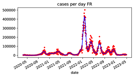
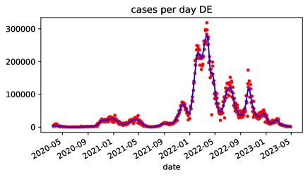
Figure 1: Number of new Covid-19 infections reported each day in France (top) and Germany (bottom) as a function of the date. The dots show the daily numbers (weekdays). As the data are very noisy the curves show the data smoothed by locally weighted smoothing followed by a cubic spline interpolation to get a set of data on a regular grid for further analysis.

The general patterns are the same in both countries, in spite of some differences in the rules imposed to contain the propagation of the epidemic such as travel restrictions and regulations restricting shopping or mandating face-masks for instance. Until the beginning of 2022 the peaks are smaller and broader than in 2022 and 2023, and the interval between them is of the order of 130–150 days. From the beginning of 2022, the peaks become much more intense and their intervals decay to values of the order of 90–95 days, and may even drop around 70 days. The peaks cannot be associated to surges due to cold seasons since there are maxima in April 2021, August 2021, April 2022, July 2022 in France and April 2021, early September 2021, April 2022, July 2022 in Germany. Therefore Covid-19 outbursts are different from the seasonal outbursts observed nowadays for influenza.

To get a more quantitative and systematic view of the dynamic of the epidemics in the two countries, we made a time-frequency analysis of the data by means of the Wigner-Ville (WV) transform Bouachache and Flandrin (1985); Flandrin and Bernard (1985); pyt applied to the smoothed and interpolated data plotted as continuous curves in Fig. 1. This transform can be viewed as an improved version of the short-term Fourier transform to detect frequencies present in a signal in a finite time domain. It is appropriate for non-stationary signals and reduces the effect of the crippling compromise between the resolution in time and frequency Bouachache and Flandrin (1985); Flandrin and Bernard (1985). Owing to its broad use in signal processing software packages implementing a discrete-time version of the WV transform pyt have been developed.

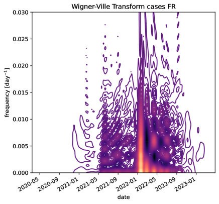
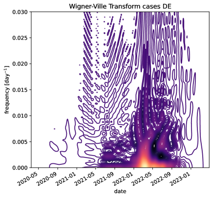
Figure 2: Time-frequency analysis of the smoothed and interpolated data plotted as continuous curves in Fig. 1, using the Wigner-Ville transform. The figure shows contour-plots of the modulus of the Wigner-Ville transform of the signal in France (top picture) and Germany (bottom) in the date-frequency plane. The scale extends over the full range of the modulus of the Wigner-Ville spectrum with 80 contour levels. The largest values, observed around the beginning of year 2022, are highlighted by the orange/yellow filling of the contours.

The WV spectra of the smoothed curves showing the variation versus time of the daily numbers of Covid-19 infections in France and Germany (Fig.1) are plotted in Fig. 2. The similarity of the WV time-frequency spectra in France and Germany is striking, in spite of the differences in the shapes of the time-dependent curves of Fig.1. A simple glance at those WV spectra already tells a lot on the Covid-19 infection, especially if we confront the spectra with the spread of the virus variants in Europe, well represented (up to a few days) by the knowledge for France. The first significant change, following the original $\alpha$ and $\beta$ forms, was the appearance of the $\delta$ variant, which had already caused a large epidemic in India. In France the $\delta$ variant was at the origin of 34% of the cases in June 2021 and 99% in August 2021. The Omicron variant contributed to 40% of the new infections mid-December 2021 and more than 95% in January 2022. The large extension of the WV-spectra toward high frequencies, which appears clearly at the very beginning of 2022 in France and Germany could have been guessed from the curves of Fig.1 because it is due to the strong, sharp, peaks that are observed at that time and were explained by the presence of the Omicron variant. But the detection of the arrival of $\delta$ variant would not be noticed on Fig.1, while it appears on the WV spectra by a significant rise in high-frequency contributions around June 2021 (particularly in France, but in Germany as well).

This shows that the WV-time-frequency analysis of the epidemic data may be a useful tool to follow the development of an epidemic. This result is particularly interesting to test epidemic models because it tells us that a successful model should be able to show the kind of change in the period of the recurrence of outbursts which is observed in the French and German epidemics provided its parameters are modified in a manner quantitatively consistent with the known properties of the virus variants. We show below that not all models are able to withstand this test.

III Memory effects

The basic epidemic model is the SIR model introduced and studied in details by Kermack and McKendrick who proposed an approximate solution for the profile of the epidemic Kermack and McKendrick (1927). In this model, once an individual has recovered he acquires a permanent immunity, so that the number of susceptible individuals is progressively exhausted and the infection peak dies-out completely. The infection never restarts.

One possible source of periodic outbursts is that actually immunity does not last forever. In the case of the Covid-19 disease, it disappears after a finite-time interval. This introduces a memory effect in the dynamics of the epidemic, which can lead to recurrences. An extension of the SIR model to take into account this finite-time immunity was recently introduced by Bestehorn et al. Bestehorn et al. (2022). We implemented this model to test its suitability to describe the dynamics of the Covid-19 epidemics in France and Germany. This section presents our results after a brief introduction to the model.

III.1 The extended SIR model with memory

Let us denote by $S$, $I$ and $R$ the fraction of susceptible, infected and recovered individuals in the total population so that $S+I+R=1$. The simple SIR model assumes that an infection occurs with rate $\beta$ when an infectious person and a susceptible individual come into contact, and that an infected individual recovers (or more precisely stops being infectious) after an average time $\gamma$. The dynamics of the model versus time $t$ is, therefore, described by the set of equations

$$\frac{dS}{dt}=-\beta\,I\,S,\quad\frac{dI}{dt}=\beta\,I\,S-\gamma I,\quad\frac{dR}{dt}=\gamma I\;.$$ (1)

It is convenient to introduce a dimensionless time $t^{\prime}=t/\gamma$ and the basic reproduction number $\rho=\beta/\gamma$, so that, in these units, the model depends on the single parameter $\rho$

$$\frac{dS}{dt^{\prime}}=-\rho\,I\,S,\quad\frac{dI}{dt^{\prime}}=\rho\,I\,S-I,\quad\frac{dR}{dt^{\prime}}=I\;.$$ (2)

We, henceforth, drop the prime for the time. It is understood that the unit of time is the average time needed for an individual to recover.

The model with memory assumes that an individual who recovered at time $t$ loses its immunity after a delay $\tau$ with probability $K(\tau)$ and becomes susceptible again. The equations are, therefore, completed by extra terms to describe the decay in the population of recovered individuals and the corresponding growth in the population of susceptible individuals.

$$\frac{dS(t)}{dt} =-\rho\,I(t)\,S(t)+\int_{0}^{\infty}I(t-\tau)K(\tau)d\tau$$ (3a)

$$\frac{dI(t)}{dt} =\rho\,I(t)\,S(t)-I(t)$$ (3b)

$$\frac{dR(t)}{dt} =I(t)-\int_{0}^{\infty}I(t-\tau)K(\tau)d\tau$$ (3c)

As suggested by Bestehorn et al. Bestehorn et al. (2022), a convenient functional form for $K(t)$ is the Erlang distribution

$$K_{\alpha,\xi}(t)=\frac{\xi^{\alpha}t^{\alpha-1}}{\Gamma(\alpha)}e^{-\xi t},\quad\alpha>0,\quad\xi>0,\quad t\geq 0$$ (4)

plotted in Fig 3. $\Gamma(\alpha)$ is the Euler $\Gamma$ function, $\alpha$ is a positive real number and $\xi$ is a scaling factor for time, with larger $\xi$ values making the distribution sharper. The maximum of the distribution, which is the typical lifetime of the immunity is reached for

$$t=\tau_{0}=(\alpha-1)/\xi\quad.$$ (5)

Figure 3: The Erlang distribution for selected values of $\alpha$ and $\xi$.

III.2 The Covid-19 infection described by the memory model

The model described by Eqs. 3 does not have an analytical solution, but it can easily be investigated by numerical simulations. We assume that the fraction of infected individuals is $I(t)=0$ for $t<0$ and $I(t=0)=I_{0}=2\,10^{-2}$, $S(t=0)=1-I_{0}$ and $R(t=0)=0$. As $I(t)$ vanishes for $t<0$, the integrals of Eqs. 3 have to be calculated in the domain $0\leq\tau<t$. We use a fourth-order Runge-Kutta algorithm to solve Eqs. 3, with a time step $dt=0.01$ in units of the recovery time $\gamma$.

The model has two stationary solutions $0\leq\overline{S}\leq 1$, $\overline{I}=0$, $\overline{R}=1-\overline{S}$ which corresponds to a healthy population and $\overline{S}=1/\rho$, $0\leq\overline{I}\leq 1-\overline{S}$ which corresponds to a stable endemic situation. For a given value of $\rho$, above a bifurcation point that can be reached by increasing $\tau_{0}$, the stable endemic point becomes unstable and this leads to a series of periodic outbursts as shown in Fig. 4

Figure 4: Fraction of susceptible individuals (dashed line, left scale) and infected individuals (full line, right scale) versus time for the memory model with $\alpha=111$, $\xi=5.0$ and $\rho=2.8$.

When $\tau_{0}$ decreases, the period between the outbursts gets shorter, and, below the bifurcation point the outbursts decay with time and the model evolves toward the endemic stable point as shown in Fig. 5.

Figure 5: Variation with time of the fraction of infected individuals for two parameter sets of the model: full line same as in Fig. 4 corresponding to $\tau_{0}=22$ (recovery time) and dashed line $\alpha=41$, $\xi=5.0$, $\rho=2.8$ corresponding to $\tau_{0}=6$ (recovery time)

Although we did not try to fit observed data because the model is too crude to pretend to be realistic, the parameters used to generate Fig. 4 have been chosen to give plausible numbers for the first stage of the epidemic in France and Germany (with $\alpha$ and $\beta$ virus variants). The recovery time $\gamma$, which is the time during which an infected individual can contaminate susceptible individuals can be estimated to be 5 days, so that the mean immunity lifetime $\tau_{0}=22$, measured in terms of the recovery time is of the order of 3.7 months with a standard deviation of about 20 days, as shown in Fig. 3 by plotting the probability distribution function for the lifetime of the immunity following the disease. The period between the outbursts on Fig. 4 is $33.37\,\times\,$the recovery time, i.e. 166.8 days, which is the order of magnitude of the time separating outbursts at the very beginning of the epidemic. Choosing parameters leading to a larger value for $\tau_{0}$, i.e. a longer immunity lifetime that is not implausible, would bring the period between the outbursts well above the observed values, which already casts a doubt on the validity of this model for the Covid-19 epidemics.

Evaluation of the model parameters that depend on the virus variant is not straightforward because many of the studies on infectivity or duration of the immunity are derived from biological parameters such as the viral load or the persistence of antibodies in the serum, rather than the influence of the variants on the epidemic itself. There are, nevertheless, some studies which provide some useful insight. A paper by Liu and Rocklöv Liu and Rocklöv (2021) compares the reproductive number for the $\delta$ variant, evaluated on average to be in the range $3.2\leq\rho\leq 8$ with a mean of $5.08$, to the value for the original strain $\rho=2.79$. This is why we selected $\rho=2.8$ for the calculation presented in Fig. 4 meant to describe the first stage of the epidemic. The lifetime of the immunity has been often evaluated for the vaccine-acquired immunity, which could be different from the immunity acquired from the disease, but may be expected to be similar. The main point for our study is that for Omicron the immunity is much shorter than for the variants present in the first stage of the epidemic Andrews et al. (2022). It decreases very significantly after 10 weeks, but many cases of multiple fast re-infections by Omicron have been observed. On average, taking into account the cases of individuals who hardly appeared to have any immunity we can estimate that the immunity provided by an Omicron infection does not exceed a month.

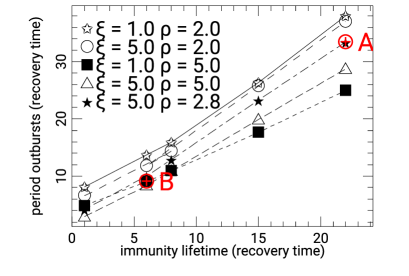
Figure 6: Results for the memory model for a variety of parameters. The values of $\xi=1$ and $\xi=5$, illustrate the effect of the sharpness of the distribution of the lifetime of the immunity. The value $\xi=5$, which leads to a standard deviation of about 3 weeks for the lifetime of the immunity is the most relevant for the Covid-19 epidemic. The reproduction number $\rho$ determines the average number of new infections generated by an infectious person. It was estimated to be $\rho\approx 2.8$ for the ancestral strain of the virus and to rise to $\rho\approx 5$ for the $\delta$ variant Liu and Rocklöv (2021), and is probably of the same order for Omicron. The lines connect data with the same $\xi$ and $\rho$ values, but a varying immunity lifetime $\tau_{0}$ obtained by varying $\alpha$ according to Eq. (5). The points marked A and B show the parameters chosen as appropriate to simulate first and second stages of the Covid-19 epidemic.

Figure 6, which shows how the period of the outbursts varies with the lifetime of the immunity in the case of the memory model can be used to analyze the validity of this model for the Covid-19 epidemic in France and Germany. First, one should notice that the sharpness of the distribution of immunity lifetimes is not a crucial feature. For $\rho=2$, the periodicities of the outbursts for $\xi=1$ (open stars, broad distribution) and $\xi=5$ (open circles, sharper, more realistic distribution) are almost the same and only differ slightly for the shortest immunity lifetimes. For $\rho=5$, the results (closed squares and open triangles) differ a bit more but nevertheless not very much. To describe the two stages of the epidemic observed in France and Germany, the relevant points are points A ($\xi=5$, $\rho=2.8$, $\tau_{0}=22\,\times\,$ the recovery time, i.e. $\approx 3.7$ months corresponding to $\alpha$ or $\beta$ virus variants) that gives a period of $P_{1}=33.37\,\times\,$the recovery time, i.e. $P_{1}\approx 167$ days, and B ($\xi=5$, $\rho=5$, $\tau_{0}=6\,\times\,$the recovery time, i.e. $\approx 30$ days, corresponding to Omicron) that gives a period $P_{2}=9.07\,\times\,$the recovery time, i.e. $P_{2}\approx 45$ days. The ratio $P_{1}/P_{2}\approx 3.7$ is much higher than the ratio of less than 2 that is observed when Omicron replaces earlier variants in France and Germany. Moreover, as observations have shown that the Omicron infection offers a very weak protection against a resurgence of the disease for an individual, our estimate of $30$ days for the lifetime of the Omicron immunity is probably an overestimate, while the immunity lifetime for the original virus strain and $\alpha$ and $\beta$ variants that we selected to be $3.7$ months may be underestimated. Therefore the ratio $P_{1}/P_{2}$ provided by the memory model could probably be even higher. In fact Fig. 6 shows that, for a given $\rho$ the period of the outbursts predicted by the model is almost proportional to the immunity lifetime, which is the the basic idea behind the memory model. As the observation of the epidemics has shown that the immunity provided by the Omicron infection is very much weaker than the immunity provided by the initial strains of the virus, it could have been predicted that the memory model should lead to a very large change in the dynamics of the epidemics when the Omicron variant started to dominate. The observations do not show such a large a qualitative transition in the periods of the outbursts, suggesting that the memory effect due to the lifetime of the immunity is not at the origin of the periodic outbursts for the Covid-19 epidemics although one can find some model parameters that appear to fit a few successive outburst of a Covid epidemic Bestehorn et al. (2022). Testing the evolution due to the virus variants provides a harder test that the model does not seem to be able to pass with parameters that stay in a realistic range.

IV Cluster saturation

Another approach was recently put forward by Gostiaux et al. Gostiaux, Bos, and Bertoglio (2023) to explain periodic epidemic outbursts with an extension of the SIR model. The idea is that the propagation of the disease does not affect the population globally but instead that it is controlled by the events in local clusters that interact weakly with the global population that plays the role of a reservoir. In this approach a SIR-like model is written at the level of a cluster. Some of the individuals who recover within the cluster can be transferred to a group of recovered individuals in the general population while some members of the general population, who had not yet been affected by the disease can join the group of susceptible individuals of the cluster, which, therefore, tends to grow. This last hypothesis is actually the crucial point, which is at the origin of periodic outbursts.

In fact the idea that the growth of the group of the susceptible individuals was behind periodic outbursts of an epidemic was already introduced in 1929 by Soper who studied “The interpretation of periodicity in disease prevalence” Soper (1929). He was investigating the measles epidemics, and wrote: “that the accumulation of susceptibles – since more than 90% of all children born in Western Europe and surviving infancy pass through an attack of measles – is an important factor of the oscillations or periods of the epidemics has been adopted by the great majority of epidemiologists”. Then he presented an analysis showing that the growth of the number of susceptible individuals is enough to give rise to periodic oscillations. In his paper he considered several models because, for measles, the infectious period is short and follows a larger period of incubation. But, in the simplest case where the infectious period can be assumed to extend during the whole illness, Soper came to a model that is analogous to the SIR model completed by a single term that generates a continuous growth of the population of susceptible individuals. With our notations, Soper’s model is described by the equations

$$\frac{dS(t)}{dt} =-\rho\,I(t)\,S(t)+\epsilon$$ (6a)

$$\frac{dI(t)}{dt} =\rho\,I(t)\,S(t)-I(t)$$ (6b)

when the time is measured in units of the recovery time. For measles the extra term $\epsilon$ added to the first equation of the SIR model was simply explained by the birth rate of children in a given area (typically an English city) affected by periodic outbursts of measles. In the context of the Covid-19 epidemic, we, henceforth, call this model the “cluster model” because it can be viewed as a simplified version of the model of Gostiaux et al. Gostiaux, Bos, and Bertoglio (2023). It should be understood as the model of a sub-population (the “cluster”) that is in contact with a broader reservoir of population. In their approach Gostiaux et al. described the interaction as a diffusion process in two dimensions, with a cluster population viewed as proportional to the area of the domain covered by the sub-population and a rate of change that is determined by the displacement of the perimeter of the domain. In two-dimensional diffusion a segment of the perimeter moves as $\sqrt{t}$ so that the area of the domain grows proportionally to $t$. This growth corresponds to $dS/dt=\epsilon$, where $\epsilon$ is simply the proportionality constant, hence the term added to the SIR model in Eq. (6a).

In this section we show that this highly simple model, with very few parameters, is sufficient to explain important observations on the Covid-19 epidemics.

Figure 7: Fraction of susceptible individuals (dashed line, left scale) and infected individuals (full line, right scale) versus time for the cluster model with $\rho=2.8$ and $\epsilon=0.012$. The horizontal long-dashed thin lines show the values corresponding to the fixed point $\overline{S}=1/\rho$ and $\overline{I}=\epsilon$.

Figure 7 shows the variation versus time of the fraction of susceptible (dashed lines) and infected (full line) individuals computed by the cluster model with $\rho=2.8$ and $\epsilon=0.012$. As for the memory model the simulation was carried out by a numerical integration of Eqs (6) with a fourth-order Runge-Kutta algorithm with a time step $dt=0.01$ in units of the recovery time. The initial condition assumes a fraction of infected individuals $I(t=0)=I_{0}=2\,10^{-2}$, $S(t=0)=1-I_{0}$ and $R(t=0)=0$. The model gives a sequence of successive outbursts that decay as time grows. The pattern is qualitatively similar to the series of outbursts observed in France and Germany in 2022 and 2023 (Figs. 1). In the long term the calculation reaches an endemic state with a small fraction of infected individuals. Each outburst is preceded by a quasi-linear growth of the fraction of susceptible individuals, which drops sharply when an outburst occurs, before growing again.

In spite of the apparent simplicity of the model, we could not derive an analytical solution to the set of nonlinear equations (6). However some of the main features of the numerical solution can be deduced from these equations.

First, the model has a fixed point $\overline{I}$ given by

$$\frac{d\overline{S}}{dt}=0=-\rho\overline{S}\;\overline{I}+\epsilon\;,\quad\frac{d\overline{I}}{dt}=0=\rho\overline{S}\;\overline{I}-\overline{I}$$ (7)

corresponding to $\overline{I}=\epsilon$ and $\overline{S}=1/\rho$ which are shown by long-dashed horizontal lines on Fig. 7.

Due to the analogy between the SIR model and the cluster model, the dynamics of an outburst can be approximately described by the solution obtained by Kermack and McKendrick Kermack and McKendrick (1927) for the SIR model in the limit $\rho R\ll 1$. Using the third equation in Eqs. (1), the first of these equations becomes $dS/dt=-\rho S\;dR/dt$. Using the initial condition $R(t=0)=0$, $S(t=0)=S_{0}$ $I_{0}=1-S_{0}$, one obtains

$$S=S_{0}e^{-\rho R}\,$$ (8)

and then, in the case $\epsilon=0$ Kermack and McKendrick could use the condition $I+S+R=1$ so that the third equation of Eq. 1 finally gives

$$\frac{dR}{dt}=1-S_{0}e^{-\rho R}-R\;.$$ (9)

This nonlinear differential equation for $R(t)$ cannot be solved exactly, but, in the limit $\rho R\ll 1$, expanding the exponential up to second order gives

$$\frac{dR}{dt}=1-S_{0}+(\rho S_{0}-1)R-\frac{1}{2}\rho^{2}S_{0}R^{2}\;.$$ (10)

A second order expansion was required because $\rho R$ has to be compared to $1-S_{0}=I_{0}$ which is itself small. Equation (10) has the solution Kermack and McKendrick (1927)

$$R(t)=\frac{1}{\rho^{2}S_{0}}\left[\rho S_{0}-1+\nu\tanh\left(\frac{\nu t}{2}-\phi\right)\right]\;,$$ (11)

with $\nu^{2}=(\rho S_{0}-1)^{2}+2S_{0}I_{0}\rho^{2}$ and $\phi=\tanh^{-1}[(\rho S_{0}-1)/\nu]$. This gives the shape of an outburst as

$$\frac{dR(t)}{dt}=I(t)=\frac{\nu^{2}}{2\rho^{2}S_{0}}\mathrm{sech}^{2}\left(\frac{\nu t}{2}-\phi\right)\;.$$ (12)

Figure 8: Fraction of susceptible individuals (short-dashed line, left scale) and infected individuals (full line, right scale) versus time for the cluster model with $\rho=1.1$ and $\epsilon=2.5\,10^{-4}$. The horizontal long-dashed line shows the value of the fixed point for the fraction of susceptible individuals $\overline{S}=1/\rho$. The thick gray full line shows the theoretical solution for the SIR model in the limit $\rho R\ll 1$.

Figure 8 shows that the theoretical shape of the outbursts derived for the SIR model in the limit $\rho R\ll 1$ provides a fairly good description of the numerical result obtained for the cluster model for a small value of $\epsilon=2.5\,10^{-4}$. This shows that the analytical results of Kermack and McKendrick Kermack and McKendrick (1927) for the SIR model can be used to get some insight into the properties of the cluster model. The important point of their analytical investigation, besides the shape of the outbursts, is that it shows that the epidemic outburst is triggered by a threshold in the fraction of susceptible individuals, which, for the SIR model is equal to $\widetilde{S}=1/\rho$. The simulation results (Fig. 8) indicate that there is still a threshold for $\epsilon\not=0$. However its value is moved up to $\widetilde{S^{\prime}}=1/\rho+\widetilde{\Delta S}$. This is the existence of this threshold that explains the periodicity of the outbursts for $\epsilon\not=0$. The term $\epsilon$ in $dS/dt$ causes a growth of $S(t)$ until it reaches the threshold and triggers an epidemic outburst. The outburst induces a quick drop in $S(t)$, which brings it below the threshold, down to a value approximately equal to $1/\rho-\widetilde{\Delta S}$. After the outburst the growth of $S(t)$ restarts until the threshold is again reached, causing the next outburst, and so on. For larger values of $\epsilon$, the analytical result of Kermack and McKendrick, 1927 is no longer quantitatively valid. Figure 7 shows that the threshold $\widetilde{S^{\prime}}$ tends to decrease from one outburst to the next, presumably because it depends on the value of $I(t)$ at the end of the previous outburst.

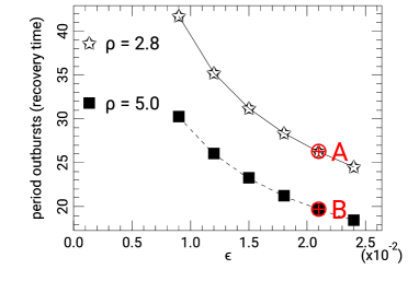
Figure 9: Results for the cluster model for a variety of parameters. The two values of $\rho$ correspond to the estimated values of the average number of new infections generated by an infectious person in the first stage ($\rho=2.8$) and second stage of the Covid-19 epidemic ($\rho=5$) Liu and Rocklöv (2021). The figure shows how the period of the outbursts depend on $\epsilon$ for those two values of $\rho$. Points A and B mark the parameters appropriate for the first and second stage of the epidemic.

Figure 9 shows how the period of the outbursts, measured in units of the recovery time, depends on $\epsilon$ for the two values $\rho=2.8$ and $\rho=5$ corresponding to first and second stages of the Covid-19 epidemic (see Sec. III and Liu and Rocklöv (2021)). For a fixed $\widetilde{S^{\prime}}$ threshold, the period should decrease linearly with the increase of $\epsilon$. A weak deviation from linearity, observed on Fig. 9, occurs because $\widetilde{S^{\prime}}$ depends on $\epsilon$.

The parameter $\epsilon$, which determines the growth of the number of susceptible individuals in a cluster, is a measure of the interactions between people in the society. We can assume that, on average, it did not vary significantly during the full epidemic, and moreover, as social behaviors are similar in France and Germany, we can select the same value of $\epsilon$ for the two countries. Selecting $\epsilon=0.021$ corresponds to the points A (first stage of the epidemic, $\rho=2.8$) and B (second stage, $\rho=5$) marked on Fig. 9. With this value of $\epsilon$, the periods of the outbursts determined by the cluster model are $P_{1}=26.23\,\times\,$the recovery time, i.e. $P_{1}\approx 131$ days for the first stage of the epidemic and $P_{2}=19.67\,\times\,$the recovery time, i.e. $P_{2}\approx 98$ days for the second stage. These two numbers are in good agreement with the numbers observed in France and Germany, and, contrary to what we had noticed for the memory model, $P_{1}/P_{2}\approx 1.34$ is consistent with the observations. It should be stressed that, owing to the simplicity of the cluster model that only has two parameters $\rho$ and $\epsilon$, there is little room to fiddle with parameters to reach an agreement between the theory and experiment. The values of $\rho$ in both stages of the epidemic result from medical observations Liu and Rocklöv (2021). They are certainly not perfectly accurate, but they are in line with the observations in various countries. The only free parameter of the model is $\epsilon$. Changing $\epsilon$ modifies $P_{1}$ and $P_{2}$ as shown in Fig. 9, but the ratio $P_{1}/P_{2}$ stays almost constant. Therefore there is actually no freedom for data fitting. Once $\epsilon$ is chosen to get a correct value of $P_{1}$, then $P_{2}$ is determined. As the model, with realistic values for $\rho$, gives a ratio $P_{1}/P_{2}$ which agrees with the observations, it strongly suggests that the mechanism behind the periodic outbursts of the Covid-19 epidemics is the growth of the clusters of affected individuals, due to social contacts, rather than the finite duration of the immunity to the virus provided by the disease (or by vaccines) as assumed for the memory model.

V Discussion

Although a large number of investigations have been devoted to the modeling of epidemics, some basic questions remain open. Accurate modeling of specific events requires a very accurate description, involving many intricate phenomena, and, therefore, many parameters that have to be fitted. Such models may help in managing epidemic containment and disease treatment. However, the difficulty is sometimes to identify the real cause behind the observations.

This is the case for the periodic outbursts of epidemics. Seasonal factors have been invoked, but they do not apply to the dynamics of Covid-19 epidemics observed in Europe (Sec. II). Moreover historic studies of the influenza epidemics, which are now seasonal through the world, have shown that earlier epidemics in Iceland did not have such a seasonal character Weinberger et al. (2012) indicating that the phenomena may be subtle. Two main ideas to explain the periodic outbursts of the Covid-19 epidemics have recently been explored. One relies on the finite duration of the acquired immunity Bestehorn et al. (2022), while the second considers the role of epidemic clusters Gostiaux, Bos, and Bertoglio (2023). Determining which one is the appropriate mechanism is not easy because it is always possible to find a parameter set that can match one observed periodicity.

However we have shown that the dynamics of the Covid-19 epidemics in France and Germany is more complex than a single periodicity. In any case, due to the many phenomena that enter into play we should not expect a single, well-defined period for the outbursts. However the data in both countries show a clear pattern of periodicity change, correlated to the appearance of new virus variants (Sec. II). In a first stage of the epidemics, with the original virus strain or $\alpha$ or $\beta$ variants, the periodicity of the outbursts was about $1.3$–$1.5$ times longer than during the second stage with the $\delta$ and Omicron variants. This observation is valid for two independent data sets for France and Germany, and the transition between the two stages is clearly visible in a time-frequency analysis of the infection data. This provides a clear signal that might discriminate between the possible models.

We used two models that have a small number of parameters. Moreover these parameters, such as the duration of the acquired immunity, or the number of individuals contaminated by somebody who had been infected, can be rather accurately estimated from the medical data. Our results show that the duration of the acquired immunity is unlikely to explain the observations because the properties of the Omicron variant that dominates the second stage of the epidemic are so much different from those of the original strain or of the $\alpha$ and $\beta$ variants that they would lead to a change in the periodicity which is much larger than the factor $1.3$–$1.5$ that is observed (Sec. III). Instead a model based on the limited size of epidemic clusters, which may grow by exchange with the reservoir provided by the general population, appears to give a rather good agreement with the observations, suggesting that the ideas behind this model are the source of the Covid-19 periodic outbursts (Sec. IV). As this model is very simple, with only two parameters, one being determined by medical data and the second controlling the periods in the two stages but not their ratio, there is very little room to fiddle with parameters to reach an agreement with the observations.

The results leave us with several points to keep in mind.

$\bullet$ Do not forget old studies! The SIR model for epidemics, which is behind many recent investigations, has been thoroughly studied in 1927 by Kermack and McKendrick Kermack and McKendrick (1927). And the “cluster model” had already been introduced by Soper in 1929 in a different context Soper (1929) when he studied measles epidemics in England. The study of Soper, who showed how the periodicity of the outbursts of measles epidemics could be related to the growth of the number of susceptible individuals, appears to be of broader validity. The notion of “cluster” was also considered more than half a century ago in the case of measles by Bartlett Bartlett (1957). He showed how the periodicity of measles epidemics was varying according to the community size by studying the case of many English cities. For his analysis, Bartlett had introduced a cell model, with diffusion between cells, so that the essential features of the cluster model of Gostiaux et al. Gostiaux, Bos, and Bertoglio (2023) were contained in his approach. His work shows that, while the epidemics tend to fade away in small communities, the disease tends to stay in an endemic state when a community gets large enough, as it does in the simple cluster model that we investigated. Considering the large degree of exchanges that take place now-days in the world, the lesson of history is not optimistic concerning eradication of the Covid-19 disease. Fortunately modern vaccination could alter the course of the events!

$\bullet$ Small is beautiful. It is always tempting to set up complex models because they can be realistic. The models that we explore, and particularly Soper’s model used as a simplified cluster model, would not be able to reproduce the curves that we showed in Sec. II, but if we focus on a specific feature of the data, which is generic and not trivial to reproduce while taking realistic constraints into account, the very small number of model parameters is an important strength because it does not allow to play with the parameters to describe the observations. This is a reminder of the famous sentence attributed to J. von Neumann by E. Fermi: “With four parameters I can fit an elephant, and with five I can make him wiggle his trunk.”Dyson (2004).

$\bullet$ Attributing the Covid-19 outbursts to the parameter $\epsilon$ of the cluster models may be tested by other studies. This parameter actually measures the degree of contacts within the society. Therefore it must actually vary depending on some specific situations, such as vacancies causing more travel or celebrations that tend to bring families together like Christmas. A statistical analysis of the Covid-19 data to try to correlate them to such events could help support the “cluster model”. Such a study must, however, be made with care. There are examples showing that people gathering can lead to Covid-19 outbursts, such a religious gathering in France and of the “Rosenmontag” period in Germany in the early stage of the Covid-19 epidemic. A correlation of a single outburst with a gathering is a trivial effect and only sufficient statistics on the fluctuations of the intervals between outbursts could be meaningful. Moreover small fluctuations of $\epsilon$ due to external conditions extending to a full country (such as the date of the beginning of the virus spreading, or the dates of the school vacations) could contribute to synchronize the evolutions in different clusters. Otherwise, if the clusters were small at the scale of a country and independent from each other, various local outbursts would average out and no clear periodicity would be seen.

$\bullet$ Finally one can point out that, although the memory model and the cluster model lead to different conclusions about the origin of the periodicity in Covid-19 outbursts they actually share the same fundamental feature: outbursts appear when the concentration of susceptible individuals has sufficiently grown. In the memory model the growth is due to the loss of immunity of previously immunized individuals, while in the cluster model it occurs because new individuals come into contact with the cluster. Nevertheless behind both models one finds the idea first introduced in a model by Soper Soper (1929).