A Bayesian Non-parametric Approach to Generative Models: Integrating Variational Autoencoder and Generative Adversarial Networks using Wasserstein and Maximum Mean Discrepancy

Abstract

Generative models have emerged as a promising technique for producing high-quality images that are indistinguishable from real images. Generative adversarial networks (GANs) and variational autoencoders (VAEs) are two of the most prominent and widely studied generative models. GANs have demonstrated excellent performance in generating sharp realistic images and VAEs have shown strong abilities to generate diverse images. However, GANs suffer from ignoring a large portion of the possible output space which does not represent the full diversity of the target distribution, and VAEs tend to produce blurry images. To fully capitalize on the strengths of both models while mitigating their weaknesses, we employ a Bayesian non-parametric (BNP) approach to merge GANs and VAEs. Our procedure incorporates both Wasserstein and maximum mean discrepancy (MMD) measures in the loss function to enable effective learning of the latent space and generate diverse and high-quality samples. By fusing the discriminative power of GANs with the reconstruction capabilities of VAEs, our novel model achieves superior performance in various generative tasks, such as anomaly detection and data augmentation. Furthermore, we enhance the model’s capability by employing an extra generator in the code space, which enables us to explore areas of the code space that the VAE might have overlooked. With a BNP perspective, we can model the data distribution using an infinite-dimensional space, which provides greater flexibility in the model and reduces the risk of overfitting. By utilizing this framework, we can enhance the performance of both GANs and VAEs to create a more robust generative model suitable for various applications.

Keywords: Dirichlet process, generative models, variational autoencoders, computational methods.

1 Introduction

The original GAN, also known as Vanilla GAN, was introduced by Goodfellow et al. (2014), and since then, various types of adversarially trained generative models have been developed. These models have exhibited outstanding performance in creating sharp and realistic images by training two neural networks concurrently, one for generating images and the other for discriminating between authentic and counterfeit images. These networks are trained in an adversarial manner until the discriminator cannot distinguish between real and fake samples.

Despite GANs being a powerful class of deep-learning models, they still face some notable challenges including mode collapse and training instability. The mode collapse issue in GANs occurs when the generator starts to memorize the training data instead of learning the underlying patterns of the data. This results in the generator becoming too specialized in generating the same samples repeatedly, which leads to a lack of diversity in the generated samples. Instability in GANs occurs when the generator and the discriminator are incapable of converging to a stable equilibrium (Kodali et al., 2017). A significant factor contributing to these issues is the tendency of the gradients used to update network parameters to become exceedingly small during the training process, causing the vanishing gradient that leads to a slowdown or even prevention of learning (Arjovsky and Bottou, 2017).

Unlike GANs, VAEs use a probabilistic approach to encode and decode data, enabling them to learn the underlying distribution and generate diverse samples, albeit with some blurriness. Consequently, the integration of GAN and VAE models has garnered significant attention as an intriguing idea for generating high-quality and realistic datasets. This approach allows for the full exploitation of the strengths of both generative models while mitigating their shortcomings.

In spite of the availability of numerous frequentist generative models, developing a BNP-based procedure poses a considerable challenge. Frequentist GANs, in particular, consider a specific form for the distribution of the data, which can lead to overfitting. This means that the generator may fit the training data too closely and not be able to generalize well to new data. In contrast, BNP methods can reduce overfitting in GANs by permitting the generator to adapt to the complexity of the data without overfitting to a pre-specific distribution. BNP models use stochastic priors that can accommodate infinite parameters, allowing them to capture complex patterns in the data and provide more accurate and reliable results.

Recently, there has been an attempt to train GANs within the BNP framework, which has been proposed in Fazeli-Asl et al. (2023). The authors identified the limitations of using some frequentist techniques in training GANs. Instead, they placed a Dirichlet process (DP) prior to the data distribution and suggested a semi-BNP MMD two-sample test to train the GAN generator. The effectiveness and superiority of the proposed test were evaluated on various benchmark datasets and compared to the classical MMD test used in Li et al. (2015). The results demonstrated enhanced statistical power and reduced false positive rates of the proposed test. Furthermore, the sample generated by the semi-BNP MMD GAN was shown to be exceptional compared to its frequentist counterpart. To the best of our knowledge, this is one of the few BNP works in this area, and thus it represents a significant contribution to the field.

This paper proposes a novel hybrid generative model that integrates a GAN, a VAE, and a code generator from the BNP perspective. The GAN serves as the primary component of our model, while the VAE and the code generator are included to enhance its capabilities. Specifically, we develop this model to extend the capability of semi-BNP MMD GAN in generating high-resolution medical datasets. To achieve this, we first develop a stochastic representation of the Wasserstein distance using DP inferences. This allows us to estimate the distance between a random probability measure and a fixed distribution, which we then incorporate into the semi-BNP MMD loss function. By considering both the Wasserstein and MMD loss functions, our proposed model benefits from both overall distribution comparison and feature matching techniques, leading to reduced mode collapse and improved training outcomes.

To ensure training stability, we include a gradient penalty term to the generator loss, following the approach proposed by Gulrajani et al. (2017). Additionally, to generate diverse samples, we replace the GAN generator with the decoder of a VAE model. Furthermore, we employ an additional generator in the code space to generate more sample codes. The code GAN serves to complement the VAE by exploring untapped areas of the code space, ensuring a more comprehensive coverage and avoiding mode collapse. Overall, our proposed approach effectively enhances the quality and visualization of the generated outputs, making it suitable for high-resolution medical image generation.

The structure of the paper is organized as follows: In Section 2, we provide an overview of the background materials in GANs, VAEs, and BNP. Next, in Section 3, we introduce a probabilistic method for calculating the Wasserstein distance using a DP prior. Then, in Section 4, we introduce our BNP-based model for integrating a GAN and a VAE. Afterwards, in Section 5, we provide experimental results from our novel generative model. Lastly, we conclude our paper in Section 6 and provide some new directions based on the research presented in this paper.

2 Background Materials

2.1 Vanilla GAN

The GAN can be mathematically represented as a minimax game between a generator network $Gen_{\boldsymbol{\omega}}$, which maps from the latent space $\mathbb{R}^{p}$ to the data space $\mathbb{R}^{d}$, $p<d$, and a discriminator network $Dis_{\boldsymbol{\theta}}$, which maps from the data space to the interval $[0,1]$. Specifically, discriminator outputs represent how likely the generated sample is drawn from the true data distribution. In the vanilla GAN, the generator tries to minimize the probability that the discriminator correctly identifies the fake sample, while the discriminator tries to maximize the probability of correctly identifying real and fake samples (Goodfellow et al., 2014). For a real sample $\mathbf{X}$ from data distribution $F$, this can be expressed as the objective function

$$\arg\min\limits_{\boldsymbol{\omega}}\max\limits_{\theta}\mathcal{L}(Gen_{\boldsymbol{\omega}},Dis_{\boldsymbol{\theta}}),$$

where $\mathcal{L}(Gen_{\boldsymbol{\omega}},Dis_{\boldsymbol{\theta}})=E_{F}[\ln(Dis_{\boldsymbol{\theta}}(\mathbf{X}))]+E_{F_{\mathbf{Z}}}[\ln(1-Dis_{\boldsymbol{\theta}}(Gen_{\boldsymbol{\omega}}(\mathbf{Z})))],$ $F_{\mathbf{Z}}$ is the distribution of the noise vector $\mathbf{Z}$, and $\ln(\cdot)$ denotes the natural logarithm. Throughout the paper, it is assumed that $F_{\mathbf{Z}}$ follows a standard Gaussian distribution.

GAN models are frequently customized by modifying the generator loss, $\mathcal{L}_{\text{Gen}}(\boldsymbol{\omega})$, and discriminator loss, $\mathcal{L}_{\text{Dis}}(\boldsymbol{\theta})$, functions. To facilitate fair comparisons among different GAN models, we reformulate the vanilla GAN objective function as a sum of $\mathcal{L}_{\text{Gen}}(\boldsymbol{\omega})$ and $\mathcal{L}_{\text{Dis}}(\boldsymbol{\theta})$ by defining

$$\mathcal{L}_{\text{Gen}}(\boldsymbol{\omega}) =E_{F_{\mathbf{Z}}}[\ln(1-Dis_{\boldsymbol{\theta}}(Gen_{\boldsymbol{\omega}}(\mathbf{Z})))],$$ (1)

$$\mathcal{L}_{\text{Dis}}(\boldsymbol{\theta}) =-E_{F}[\ln(Dis_{\boldsymbol{\theta}}(\mathbf{X}))]-E_{F_{\mathbf{Z}}}[\ln(1-Dis_{\boldsymbol{\theta}}(Gen_{\boldsymbol{\omega}}(\mathbf{Z})))],$$ (2)

respectively. Now, the vanilla GAN is trained by iteratively updating $\boldsymbol{\omega}$ and $\boldsymbol{\theta}$ using stochastic gradient descent to minimize the loss functions (1) and (2), respectively. The GAN is considered to have learned when the generator can produce samples that are indistinguishable from the real samples, and the discriminator cannot differentiate between them.

2.2 Mode Collapse in GANs

To mitigate mode collapse and enhance the stability property in GANs, Salimans et al. (2016) proposed using a batch normalization technique to normalize the output of each generator layer, which can help reduce the impact of vanishing gradients.The authors also implemented mini-batch discrimination, an additional technique to diversify the generated output. This involves computing a pairwise distance matrix among examples within a mini-batch. This matrix is then used to augment the input data before being fed into the model.

Another strategy, widely suggested in the literature to overcome GAN limitations, is incorporating statistical distances into the GAN loss function. Arjovsky et al. (2017) suggested updating GAN parameters by minimizing the Wasserstein distance between the distribution of the real and fake data (WGAN). They noted that this distance possesses a superior property compared to other measures like Kulback-Leibler, Jenson Shanon, and total variation measures. This is due to its ability to serve as a sensible loss function for learning distributions supported by low-dimensional manifolds. Arjovsky et al. (2017) used the weight clipping technique to constrain the discriminator to the 1-Lipschitz constant. This condition ensures discriminator’s weights are bounded to prevent the discriminator from becoming too powerful and overwhelming the generator. Additionally, this technique helped to ensure that the gradients of the discriminator remained bounded, which is crucial for the stability of the overall training process.

However, weight clipping has some drawbacks. For instance, Gulrajani et al. (2017) noted that it may limit the capacity of the discriminator, which can prevent it from learning complex functions. Moreover, it can result in a “dead zone” where some of the discriminator’s outputs are not used, which can lead to inefficiencies in training. To address these issues, Gulrajani et al. (2017) proposed to force the 1-Lipschitz constraint on the discriminator in an alternative way. They improved WGAN using a gradient penalty term in the loss function to present the WGPGAN model. They showed that it helps to avoid mode collapse and makes the training process more stable.

Instead of comparing the overall distribution of the data and the generator, Salimans et al. (2016) remarked on adopting the feature matching technique as a stronger method to prevent the mode collapse in GANs and make them more stable. In this strategy, the discriminator is a two-sample test and the generator is trained to deceive the discriminator by producing images that match the features of real images, rather than just assessing the overall distribution of the data. Dziugaite et al. (2015) and Li et al. (2015) have demonstrated remarkable results by implementing this procedure using the MMD measure. Furthermore, Li et al. (2015) employed an autoencoder (AE) network to train an MMD-based GAN in the code space referred to as AE generative moment matching networks (AE+GMMNs). AE networks use deterministic mapping to compress data into a lower dimension (code space) that captures essential features of the original data. Li et al. (2015) attempted to generate code samples and reconstruct them in the data space to enhance the performance of their model. Their experiments showed that this approach led to a considerable reduction in noise in the generated samples compared to using MMD to train GAN in the data space.

2.3 Standard VAE

The VAE consists of an encoder network $Enc_{\boldsymbol{\eta}}$ that maps the input data $\mathbf{X}\sim F$ to a latent representation $\mathbf{Z}_{e}$, and a decoder network $Dec_{\boldsymbol{\gamma}}$ that reconstructs $\mathbf{Z}_{e}$ to the data space (Kingma and Welling, 2013). It uses a hierarchical distribution to model the underlying distribution of the data. More precisely, a prior distribution $F_{\mathbf{Z}}$ is first placed on the latent space, $\mathbf{Z}\sim F_{\mathbf{Z}}$, to specify the distribution of the encoder (variational distribution), $\mathbf{Z}_{e}:=\mathbf{Z}|\mathbf{X}\sim F_{Enc_{\boldsymbol{\eta}}}$, and the distribution of the decoder, $\mathbf{X}|\mathbf{Z}\sim F_{Dec_{\boldsymbol{\gamma}}}$, by reparametrization tricks. Then, the intractable data likelihood is approximated by maximizing the marginal log-likelihood:

$$\log f_{Dec_{\boldsymbol{\gamma}}}(\mathbf{x})=\log\int f_{Dec_{\boldsymbol{\gamma}}}(\mathbf{x}|\boldsymbol{z})f_{\mathbf{Z}}(\boldsymbol{z})\,d\boldsymbol{z},$$ (3)

where $f_{Dec_{\boldsymbol{\gamma}}}$ represents the density function corresponding to $F_{Dec_{\boldsymbol{\gamma}}}$. It can be shown that maximizing (3) is equivalent to minimizing:

$$\mathcal{L}_{\text{VAE}}(\boldsymbol{\eta},\boldsymbol{\gamma}) =D_{\text{KL}}\left(f_{Enc_{\boldsymbol{\eta}}}(\boldsymbol{z}|\boldsymbol{x}),f_{\mathbf{Z}}(\boldsymbol{z})\right)-E_{F_{Enc_{\boldsymbol{\eta}}}(\boldsymbol{z}|\boldsymbol{x})}\left(\log f_{Dec_{\boldsymbol{\gamma}}}(\boldsymbol{x}|\boldsymbol{z})\right)$$

$$=\mathcal{L}_{\text{Reg}}+\mathcal{L}_{\text{Rec}}$$ (4)

with respect to $\boldsymbol{\eta}$ and $\boldsymbol{\gamma}$. Here, $D_{\text{KL}}(\cdot,\cdot)$ denotes Kullback-Leibler divergence, and $\mathcal{L}_{\text{Reg}}$ and $\mathcal{L}_{\text{Rec}}$ represent the regularization and reconstruction errors, respectively. In fact, $\mathcal{L}_{\text{Rec}}$ is the cross-entropy that measures how well the model can reconstruct the input data from the latent space, while $\mathcal{L}_{\text{Reg}}$ encourages the approximate posterior to be close to the prior distribution over the latent space.

Although the latent space in VAEs is a powerful tool for learning the underlying structure of data, it can face limitations in its capacity to capture the complex features of an input image. When the latent space is not able to fully represent all of the intricate details of an image, the resulting reconstructions can be less accurate and lead to unclear outputs. They tend to distribute probability mass diffusely over the data space, increasing the tendency of VAEs to generate blurry images, as pointed out by Theis et al. (2015). To mitigate the blurriness issue in VAEs, researchers have proposed various modifications such as considering the adversarial loss (Makhzani et al., 2015; Mescheder et al., 2017) in the VAE objective, improving the encoder and decoder network architectures (Yang et al., 2017; Kingma et al., 2016), and using denoising techniques (Im et al., 2017; Creswell and Bharath, 2018). However, the methods mentioned earlier still produce images that exhibit a degree of blurriness.

Meanwhile, the idea of integrating GANs and VAEs was first suggested by Larsen et al. (2016), using the decoder in the VAE as the generator in the GAN. This model, known as the VAE-GAN, provides an alternative approach to addressing the challenges previously mentioned. The paper demonstrates the effectiveness of the VAE-GAN model on several benchmark datasets, showing that it outperforms other unsupervised learning methods in terms of sample quality and diversity. Donahue et al. (2016) and Dumoulin et al. (2016) independently proposed another similar approach in the same manner as in the paper by Larsen et al. (2016). However, their method incorporated a discriminator that not only distinguished between real and fake samples but also jointly compared the real and code samples (encoder output) with the fake and noise (generator input) samples, which sets it apart from the VAE-GAN model.

Another stronger method was proposed by Rosca et al. (2017) called $\alpha$-GAN. In this approach, the decoder in a VAE was also replaced with the generator of a GAN. Two discriminator networks were then used to optimize the reconstruction and regularization errors of the VAE adversarially. Moreover, a zero-mean Laplace distribution was assigned to the reconstruction data distribution to add an extra term for reconstruction error. This term was considered to provide weights to all parts of the model outputs. Several proxy metrics were employed for evaluating $\alpha$-GAN models. The findings revealed that the WGPGAN is a robust competitor to the $\alpha$-GAN and can even surpass it in certain scenarios. Recently, Kwon et al. (2019) proposed a 3D GAN by extending $\alpha$-GAN for 3D generations. The authors addressed the stability issues of $\alpha$-GAN and proposed a new hybrid generative model, 3D $\alpha$-WGPGAN, which employs WGPGAN loss to the $\alpha$-GAN loss to enhance training stability. They validated the effectiveness of the 3D $\alpha$-WGPGAN on some 3D MRI brain datasets, outperforming all previously mentioned models.

2.4 3D $\alpha$-WGPGAN

When $f_{Dec_{\boldsymbol{\gamma}}}(\boldsymbol{x}|\boldsymbol{z})$ in (2.3) is unknown, $\mathcal{L}_{\text{Rec}}$ cannot be employed directly in the training process. One way is assigning a specific distribution to $f_{Dec_{\boldsymbol{\gamma}}}(\boldsymbol{x}|\boldsymbol{z})$, like the Laplace distribution which is a common choice in many VAE-based procedures, and then minimize $\mathcal{L}_{\text{Rec}}$ (Ulyanov et al., 2018). However, this procedure can increase subjective constraints in the model (Rosca et al., 2017). An alternative method in approximating $f_{Dec_{\boldsymbol{\gamma}}}(\boldsymbol{x}|\boldsymbol{z})$ is to treat $Dec_{\boldsymbol{\gamma}}$ as the generator of a GAN to train the decoder by playing an adversarial game with the GAN discriminator. It guarantees the available training data is fully explored through the training process, thereby preventing mode collapse.

The 3D $\alpha$-WGPGAN uses both the above structures to present a model to generate new samples (Kwon et al., 2019). It also avoids using $D_{\text{KL}}$ in $\mathcal{L}_{\text{Reg}}$ to minimize the regularization error which often considers a simple form like a Gaussian for $f_{Enc_{\boldsymbol{\eta}}}(\boldsymbol{z}|\boldsymbol{x})$. It replaces $\mathcal{L}_{\text{Reg}}$ by a code discriminator, $CDis_{\boldsymbol{\theta}^{\prime}}$, by playing an adversarial game with $Enc_{\boldsymbol{\eta}}$ to approximate $f_{Enc_{\boldsymbol{\eta}}}(\boldsymbol{z}|\boldsymbol{x})$ such that the latent posterior matches to the latent prior $f_{\mathbf{Z}}(\boldsymbol{z})$. In fact, the code discriminator prompts the encoder to accurately encode the real distribution to the latent space, ensuring a more efficient and effective encoding process.

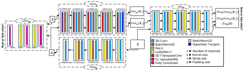
Figure 1: The general architecture of 3D $\alpha$-WGPGAN comprises three convolutional networks (encoder, generator, and discriminator) and a fully connected-based network (code discriminator).

Now, by considering the decoder as $Gen_{\boldsymbol{\omega}}$, 3D $\alpha$-WGPGAN is trained by minimizing the hybrid loss function

$$\mathcal{L}_{\text{EGen}}(\boldsymbol{\omega},\boldsymbol{\eta}) =-E_{F_{Enc_{\boldsymbol{\eta}}}(\boldsymbol{z}|\boldsymbol{x})}[Dis_{\boldsymbol{\theta}}(Gen_{\boldsymbol{\omega}}(\boldsymbol{z}_{e}))]-E_{F_{\mathbf{Z}}}[Dis_{\boldsymbol{\theta}}(Gen_{\boldsymbol{\omega}}(\boldsymbol{z}_{r}))]$$

$$~{}~{}~{}~{}+\lambda_{1}\left\|\boldsymbol{x}-Gen_{\boldsymbol{\omega}}(\boldsymbol{z}_{e})\right\|_{1},$$ (5)

$$\mathcal{L}_{\text{Dis}}(\boldsymbol{\theta}) =E_{F_{Enc_{\boldsymbol{\eta}}}(\boldsymbol{z}|\boldsymbol{x})}[Dis_{\boldsymbol{\theta}}(Gen_{\boldsymbol{\omega}}(\boldsymbol{z}_{e}))]+E_{F_{\mathbf{Z}}}[Dis_{\boldsymbol{\theta}}(Gen_{\boldsymbol{\omega}}(\boldsymbol{z}_{r}))]-2E_{F}[Dis_{\boldsymbol{\theta}}(\boldsymbol{x})],$$

$$~{}~{}~{}~{}+\lambda_{2}L_{\text{GP-Dis}}$$ (6)

$$\mathcal{L}_{\text{CDis}}(\boldsymbol{\theta}^{\prime}) =E_{F_{Enc_{\boldsymbol{\eta}}}(\boldsymbol{z}|\boldsymbol{x})}[CDis_{\boldsymbol{\theta}^{\prime}}(\boldsymbol{z}_{e})]-E_{F_{\mathbf{Z}}}[CDis_{\boldsymbol{\theta}^{\prime}}(\boldsymbol{z}_{r})]+\lambda_{2}L_{\text{GP-CDis}},$$ (7)

where $\boldsymbol{z}_{r}$ is a noise vector observed from distribution $F_{\mathbf{Z}}$. The encoder and generator create a network that is optimized using the loss function $\mathcal{L}_{\text{EGen}}(\boldsymbol{\omega},\boldsymbol{\eta})$ in (5). First terms in Equations (5) and (2.4) refer to the WGAN loss. More precisely, the objective function of WGAN is constructed as

$$\arg\min\limits_{\boldsymbol{\omega}}\mathcal{W}(F,F_{Gen_{\boldsymbol{\omega}}}),$$ (8)

where

$$\mathcal{W}(F,F_{Gen_{\boldsymbol{\omega}}})=\max\limits_{\boldsymbol{\theta}\in\Theta}E_{F}[Dis_{\boldsymbol{\theta}}(\boldsymbol{x})]-E_{F_{Gen_{\boldsymbol{\omega}}}}[Dis_{\boldsymbol{\theta}}(Gen_{\boldsymbol{\omega}}(\boldsymbol{z}))]$$ (9)

is the Wasserstein distance obtained by using the Kantorovich-Rubinstein duality in which $\Theta$ contains $\boldsymbol{\theta}$’s whose corresponding discriminators is $1$-Lipschitz (Villani, 2008). Note that Equation (9) evaluates to zero if $F=F_{Gen_{\boldsymbol{\omega}}}$.

Equation (8) is reformulated through Equations (5) and (2.4). The first expectation in Equation (9), which does not depend on $\boldsymbol{\omega}$, is not considered in the minimization gradient descent with respect to $\boldsymbol{\omega}$ and is omitted in Equation (5). As the reconstruction sample is treated as the fake data, then, the loss function (8) using $Gen_{\boldsymbol{\omega}}(\boldsymbol{z}_{e})$ is also added to the 3D $\alpha$-WGPGAN loss function. The last term in Equation (5) is the $L_{1}$-norm reconstruction loss which is obtained by assigning a Laplace distribution with mean zero and scale parameter $\lambda_{1}$ to the generator distribution in the sense that $f_{Gen_{\boldsymbol{\omega}}}(\boldsymbol{x}|\boldsymbol{z})\propto e^{-\lambda_{1}\left\|\boldsymbol{x}-Gen_{\boldsymbol{\omega}}(\boldsymbol{z}_{e})\right\|_{1}}$.

The gradient penalty $L_{\text{GP-CDis}}=E_{F_{\hat{\mathbf{X}}}}[(\left\|\nabla_{\hat{\boldsymbol{x}}}Dis_{\boldsymbol{\theta}}(\hat{\boldsymbol{x}})\right\|_{2}-1)^{2}]$ with coeficient $\lambda_{2}$ is added to Equation (2.4) to force the 1-Lipschitz constraint to the discriminator, where $\widehat{\boldsymbol{x}}=t\boldsymbol{x}+(1-t)\widetilde{\boldsymbol{x}}$, $0\leq t\leq 1$, $\widetilde{\boldsymbol{x}}$ is any generated sample by $Gen_{\boldsymbol{\omega}}$, and $F_{\widehat{\mathbf{X}}}$ is the distribution function of $\hat{\boldsymbol{x}}$. If $\boldsymbol{\theta}^{\star}$ be the optimized parameter of $Dis_{\boldsymbol{\theta}}$ that maximizes $\mathcal{L}_{W}(\boldsymbol{\theta},\boldsymbol{\omega})$, then $Dis_{\boldsymbol{\theta}^{\star}}$ should minimizes $L_{\text{GP-Dis}}$ (Gulrajani et al., 2017). The code discriminator loss in Equation (7) has the same structure as $\mathcal{L}_{\text{Dis}}(\boldsymbol{\theta})$, but with $\boldsymbol{z}_{e}$ treated as fake and $\boldsymbol{z}$ as real observed data. Kwon et al. (2019) designed the encoder and discriminator networks with five 3D convolutional layers followed by batch normalization (BatchNorm) layers and leaky rectified linear unit (LeakyReLU) activation functions.

The generator network includes a transpose convolutional (TransposeConv) layer, four 3D convolutional layers, and a BatchNorm layer with a ReLU activation function in each layer. Typically, BatchNorm and ReLU are applied to ensure network stability. The TransposeConv layer enables the network to “upsample” the input noise vector and generate an output tensor with a larger spatial resolution. The upscale layers are also implemented in the last four layers of the generator network to increase the spatial resolution of the input feature maps. The code discriminator consists of three fully connected layers followed by BatchNorm and LeakyReLU activation functions. Figure 1 provides a detailed illustration of the architecture of the 3D $\alpha$-WGPGAN.

2.5 Dirichlet Process Prior

The DP is a widely used prior in BNP methods, introduced by Ferguson (1973). It can be seen as a generalization of the Dirichlet distribution, where a random probability measure $F$ is constructed around a fixed probability measure $H$ (the base measure) with variation controlled by a positive real number $a$ (the concentration parameter). Within the context of this statement, $H$ represents the extent of the statistician’s expertise in data distribution, while $a$ denotes the level of intensity of this knowledge.

Formally, $F$ is a DP on a space $\mathfrak{X}$ with a $\sigma$-algebra $\mathcal{A}$ of subsets of $\mathfrak{X}$ if, for every measurable partition $A_{1},\ldots,A_{k}$ of $\mathfrak{X}$ with $k\geq 2$, the joint distribution of the vector $(F(A_{1}),\ldots,F(A_{k}))$ has a Dirichlet distribution with parameters $(aH(A_{1}),\ldots,aH(A_{k}))$. Additionally, it is assumed that $H(A_{j})=0$ implies $F(A_{j})=0$ with probability one. One of the most important properties of the DP is its conjugacy property, where the posterior distribution of $F$ given a sample $x$ drawn from $F\sim DP(a,H)$, denoted by $F^{pos}$, is also a DP with concentration parameter $a+n$ and base measure $H^{\ast}=a(a+n)^{-1}H+n(a+n)^{-1}F_{x}$, where $F_{x}$ is the empirical cumulative distribution function of the sample $x$. This property allows for easy computation of the posterior distribution of $F$.

Alternative definitions for DP have been proposed, including infinite series representations by Bondesson (1982) and Sethuraman (1994). The method introduced by Sethuraman (1994) is commonly referred to as the stick-breaking representation and is widely used for DP inference. However, Zarepour and Al-Labadi (2012) noted that, unlike the series of Bondesson (1982), the stick-breaking representation lacks normalization terms that convert it into a probability measure. Additionally, simulating from infinite series is only feasible with a truncation approach for the terms inside the series. Ishwaran and Zarepour (2002) introduced an approximation of DP in the form of a finite series (10), which can be easily simulated.

$$F_{N}=\sum_{i=1}^{N}J_{i,N}\delta_{Y_{i}},$$ (10)

where $(J_{1,N},\ldots,J_{N,N})\sim\mbox{Dir}(a/N,\ldots,a/N)$, and $Y_{i}\overset{i.i.d.}{\sim}H$. In this paper, the variables $J_{i,N}$ and $Y_{i}$ are used to represent the weight and location of the DP, respectively.

Ishwaran and Zarepour (2002) demonstrated that $(F_{N})_{N\geq 1}$ converges in distribution to $F$, where $F_{N}$ and $F$ are random values in the space $M_{1}(\mathbb{R})$ of probability measures on $\mathbb{R}$ endowed with the topology of weak convergence. To generate $(J_{i,N})_{1\leq i\leq N}$, one can put $J_{i,N}=H_{i,N}/\sum_{i=1}^{N}H_{i,N}$, where $(H_{i,N})_{1\leq i\leq N}$ is a sequence of independent and identically distributed $\mbox{Gamma}(a/N,1)$ random variables that are independent of $(Y_{i})_{1\leq i\leq N}$. This form of approximation has been used so far in various applications, including hypothesis testing and GANs, and reflected outstanding results. It also leads to some excellent outcomes in subsequent sections.

2.6 Maximum Mean Discrepancy Measure

The MMD measure, introduced by Gretton et al. (2012), is a kernel-based measure that evaluates the similarity between the features of samples from two high-dimensional distributions. More precisely, let $F$ and $F_{Gen_{\boldsymbol{\omega}}}$ denote the distribution of the real and fake data, respectively. Then, for given $\mathbf{X},\mathbf{X}^{\prime}\overset{i.i.d.}{\sim}F$, and $\mathbf{Y},\mathbf{Y}^{\prime}\overset{i.i.d.}{\sim}F_{Gen_{\boldsymbol{\omega}}}$, the MMD is defined by

$$MMD^{2}(F,F_{Gen_{\boldsymbol{\omega}}})=E_{F}[k(\mathbf{X},\mathbf{X}^{\prime})]-2E_{F,F_{Gen_{\boldsymbol{\omega}}}}[k(\mathbf{X},\mathbf{Y})]+E_{F_{Gen_{\boldsymbol{\omega}}}}[k(\mathbf{Y},\mathbf{Y}^{\prime})],$$ (11)

where $k(\cdot,\cdot)$ is a kernel function with feature space corresponding to a universal reproducing kernel Hilbert space. Due to the inaccessibility of $F$ and $F_{Gen_{\boldsymbol{\omega}}}$, Equation (11) is usually estimated by

$$MMD_{n,m}^{2}(F,F_{Gen_{\boldsymbol{\omega}}})=\frac{1}{n^{2}}\sum_{i\neq j}^{n}k(\mathbf{X}_{i},\mathbf{X}_{j})-\frac{2}{mn}\sum_{i=1}^{n}\sum_{j=1}^{m}k(\mathbf{X}_{i},\mathbf{Y}_{j})+\frac{1}{m^{2}}\sum_{i\neq j}^{m}k(\mathbf{Y}_{i},\mathbf{Y}_{j}),$$ (12)

using two samples $(\mathbf{X}_{1},\ldots,\mathbf{X}_{n})\sim F$ and $(\mathbf{Y}_{1},\ldots,\mathbf{Y}_{m})\sim F_{Gen_{\boldsymbol{\omega}}}$. The MMD is a non-negative measure that is zero if and only if $F$ and $F_{Gen_{\boldsymbol{\omega}}}$ are identical (Gretton et al., 2012). It can be used as a regularizer in GANs to encourage the generator to produce data that has similar features to the real dataset. Dziugaite et al. (2015) considered the loss function (13) to train the generator:

$$\arg\min\limits_{\boldsymbol{\omega}}MMD^{2}(F,F_{Gen_{\boldsymbol{\omega}}}).$$ (13)

However, Li et al. (2015) mentioned that by incorporating the square root of the MMD measure into the GAN loss function, the gradients used to update the generator can be more stable, preventing them from becoming too small and leading to gradient vanishing.

2.7 Semi-BNP MMD GAN

The Semi-BNP MMD GAN is constructed based on training a generator network by optimizing a Bayesian two-sample statistic test treated as a discriminator (Fazeli-Asl et al., 2023). Given an input data $\mathbf{X}\sim F$ and assuming a prior distribution $F^{pri}:=F\sim DP(a,H)$, the prior-based MMD distance $MMD^{2}(F^{pri},F_{Gen_{\boldsymbol{\omega}}})$ is defined using the weights and locations of the DP approximation proposed by Ishwaran and Zarepour (2002). For generated samples $\mathbf{Y}_{1},\ldots,\mathbf{Y}_{m}\sim F_{Gen_{\boldsymbol{\omega}}}$, the posterior-based MMD distance after updating from a priori to a posteriori is defined by

$$MMD^{2}(F^{pos},F_{Gen_{\boldsymbol{\omega}}}) =\sum_{\ell,t=1}^{N}J^{\ast}_{\ell,N}J^{\ast}_{t,N}k(\mathbf{V}^{\ast}_{\ell},\mathbf{V}^{\ast}_{t})-\dfrac{2}{m}\sum_{\ell=1}^{N}\sum_{t=1}^{m}J^{\ast}_{\ell,N}k(\mathbf{V}^{\ast}_{\ell},\mathbf{Y}_{t})$$

$$+\dfrac{1}{m^{2}}\sum_{\ell,t=1}^{m}k(\mathbf{Y}_{\ell},\mathbf{Y}_{t}),$$ (14)

where

$$\mathbf{V}^{\ast}_{1},\ldots,\mathbf{V}^{\ast}_{N}\overset{i.i.d.}{\sim}\frac{a}{a+n}H+\frac{n}{a+n}F_{\boldsymbol{x}},\hskip 5.69046pt(J^{\ast}_{1,N},\ldots,J^{\ast}_{N,N})\sim\mbox{Dir}(\frac{a+n}{N},\ldots,\frac{a+n}{N}),$$

and $F_{\boldsymbol{x}}$ denotes the empirical distribution of observed data. This procedure considers $k(\cdot,\cdot)$ as a mixture of Gaussian kernels using various bandwidth parameters. For instance, for a set of fixed bandwidth parameters such as $\{\sigma_{1},\ldots,\sigma_{T}\}$ and two vectors $\mathbf{V}^{\ast}_{\ell}$ and $\mathbf{Y}_{t}$, $k(\mathbf{V}^{\ast}_{\ell},\mathbf{Y}_{t})=\sum_{t^{\prime}=1}^{T}\exp\frac{-||\mathbf{V}^{\ast}_{\ell}-\mathbf{Y}_{t}||^{2}}{2\sigma_{t^{\prime}}^{2}}$.

Let density functions of the square root of the posterior and prior-based MMD measures be denoted by $\pi_{MMD}(\cdot|\mathbf{X})$ and $\pi_{MMD}(\cdot)$, respectively. The semi-BNP MMD GAN can be trained by optimizing the objective function:

$$\arg\max\limits_{\boldsymbol{\omega}}\mathrm{RB}_{MMD(F,F_{Gen_{\boldsymbol{\omega}}})}(0|\mathbf{X}),$$ (15)

where $\mathrm{RB}_{MMD(F,F_{Gen_{\boldsymbol{\omega}}})}(0|\mathbf{X})=\pi_{MMD}(0|\mathbf{X})/\pi_{MMD}(0)$ is the relative belief (RB) ratio, a Bayesian statistic that measures the change in the belief of $MMD(F,F_{Gen_{\boldsymbol{\omega}}})=0$ being true from a priori to a posteriori (Evans, 2015). A value of $\mathrm{RB}_{MMD(F,F_{Gen_{\boldsymbol{\omega}}})}(0|\mathbf{X})>1$ indicates evidence in favor of the features of the generated samples being matched to those of the real data. The generator in this procedure was implemented using the original architecture proposed by Goodfellow et al. (2014), and the model architecture is illustrated in Figure 2. Indeed, the discriminator calculates the RB ratio, and the generator should aim to maximize this value. Fazeli-Asl et al. (2023) remarked that the semi-BNP MMD GAN is equivalently trained by minimizing simple loss function: $\mathcal{L}_{Gen}(\boldsymbol{\omega})=MMD(F^{pos},F_{Gen_{\boldsymbol{\omega}}}).$

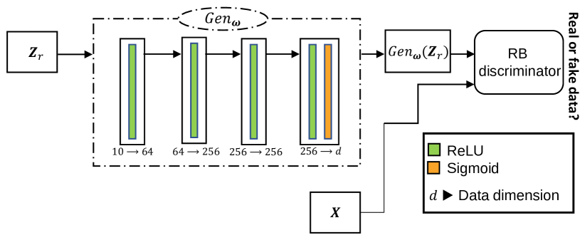
Figure 2: The general architecture of semi-BNP MMD GAN with four ReLU layers and a sigmoid activation function in the final layer.

3 A Stochastic Representation for Wasserstein Distance

In this section, we present a stochastic procedure for measuring the Wasserstein distance between a fixed probability measure and a random probability measure modeled by a DP prior. For a fixed value of $a$ and a probability measure $H$, we model the unknown data distribution $F$ as a random probability measure using the following model:

$$\mathbf{X} \sim F,$$ (16)

$$F^{pri}:=F \sim DP(a,H),$$ (17)

$$F^{pos}:=F|\mathbf{X} \sim DP(a+n,H^{\ast}),$$ (18)

where $\mathbf{X}=(\mathbf{X}_{1},\ldots,\mathbf{X}_{n})$ represent $n$ samples in $\mathbb{R}^{d}$. Let $G$ be any fixed distribution and $\{D_{\boldsymbol{\theta}}\}_{{\boldsymbol{\theta}}\in\Theta}$ be a parametrized family of continuous functions that all are 1-Lipschitz. We propose an approximation for Wasserstein between $F^{pos}$ and $G$ as

$$\mathcal{W}(F^{pos},G)=\max\limits_{\boldsymbol{\theta}\in\Theta}\sum_{i=1}^{N}\left(J^{\ast}_{i,N}D_{\theta}(\mathbf{V}_{i}^{\ast})-\dfrac{D_{\boldsymbol{\theta}}(\mathbf{Y}_{i})}{N}\right),$$ (19)

where $(J^{\ast}_{1,N},\ldots,J^{\ast}_{N,N})\sim Dir(\frac{a+n}{N},\ldots,\frac{a+n}{N})$, $\mathbf{V}^{\ast}_{1},\ldots,\mathbf{V}^{\ast}_{N}\overset{i.i.d.}{\sim}H^{\ast}$, and $Y_{1},\ldots,Y_{N}$ is a sample generated from $G$. The next theorem presents some asymptotic properties of $\mathcal{W}(F^{pos},G)$ with respect to $N,n,$ and $a$.

Theorem 1

Assuming (16)-(18), it follows that for any fixed probability distribution $G$:

• $\mathcal{W}(F^{pos},G)\xrightarrow{a.s.}\mathcal{W}(F,G)$ as $N,n\rightarrow\infty$.

• $\mathcal{W}(F^{pos},G)\xrightarrow{a.s.}\mathcal{W}(H,G)$ as $N,a\rightarrow\infty$,

where “$\xrightarrow{a.s.}$” represents almost surely convergence and $W(F,G)$ is defined in (9) with $Dis_{\boldsymbol{\theta}}=D_{\boldsymbol{\theta}}$ and $F_{Gen_{\boldsymbol{\omega}}}=G$.

Proof  Given that $E_{F^{pos}}(J^{\ast}_{i,N})=\frac{1}{N}$ for all $i\in\{1,\ldots,N\}$, we can use Chebyshev’s inequality to obtain

$$\operatorname{Pr}\left\{\left|J^{\ast}_{i,N}-1/N\right|\geq\epsilon\right\}\leq\frac{Var_{F^{pos}}(J^{\ast}_{i,N})}{\epsilon^{2}},$$ (20)

for any $\epsilon>0$. Substituting $Var_{F^{pos}}(J^{\ast}_{i,N})=\frac{N-1}{N^{2}(a+n+1)}$ into (20) and setting $n=k^{2}+b$, where $k\in\mathbb{N}$ and $b\in\{0,1,\ldots\}$, yields

$$\operatorname{Pr}\left\{\left|J^{\ast}_{i,N}-1/N\right|\geq\epsilon\right\}\leq\frac{1}{k^{2}\epsilon^{2}}.$$

The convergence of the series $\sum_{\kappa=0}^{\infty}\kappa^{-2}$ implies that $\sum_{\kappa=0}^{\infty}\operatorname{Pr}\left\{\left|J^{\ast}_{i,N}-1/N\right|\geq\epsilon\right\}<\infty$. As $k\rightarrow\infty$ or equivalently $n\rightarrow\infty$, the first Borel-Cantelli lemma implies that $J^{\ast}_{i,N}\xrightarrow{a.s.}1/N$, as required. In contrast, as $n$ approaches infinity, the Glivenko-Cantelli theorem implies that $F_{\boldsymbol{x}}$ converges to $F$ and subsequently, $H^{\ast}$ converges to $F$. This convergence indicates that the probability of drawing a sample from $F$ approaches 1. As $n\rightarrow\infty$, $\mathbf{V}_{i}^{\ast}\rightarrow\mathbf{X}_{i}$ where $\mathbf{X}_{i}$ is a random variable following distribution $F$, for $i=1,\ldots,N$. By applying the continuous mapping theorem, it follows that $D_{\boldsymbol{\theta}}(\mathbf{V}^{\ast}_{i})$ converges to $D_{\boldsymbol{\theta}}(\mathbf{X}_{i})$, as $n\rightarrow\infty$, and thus, we have

$$I=\sum_{i=1}^{N}\left(J^{\ast}_{i,N}D_{\boldsymbol{\theta}}(\mathbf{V}_{i}^{\ast})-\frac{D_{\boldsymbol{\theta}}(\mathbf{Y}_{i})}{N}\right)\xrightarrow{a.s.}\dfrac{1}{N}\sum_{i=1}^{N}(D_{\boldsymbol{\theta}}(\mathbf{X}_{i})-D_{\boldsymbol{\theta}}(\mathbf{Y}_{i})).$$ (21)

Applying the strong law of large numbers to the right-hand side of Equation (21) yields

$$I\xrightarrow{a.s.}E_{F}[D_{\boldsymbol{\theta}}(\mathbf{X}_{1})]-E_{G}[D_{\boldsymbol{\theta}}(\mathbf{Y}_{1})],$$

as $N\rightarrow\infty.$ Since $\max(\cdot)$ is a continuous function, the proof of (i) is completed by using the continuous mapping theorem. The proof of (ii) is followed by a similar approach, with $a=\kappa^{2}c$ being considered in $Var_{F^{pos}_{1}}(J^{\ast}_{i,N})$, for $\kappa\in\{0,1,\ldots\}$ and a fixed positive value of $c$.  

The next corollary demonstrates a crucial property of the $\mathcal{W}(F^{pos},G)$ metric, which makes it a convenient tool for comparing two models.

Corollary 2

Let $\{G_{k}\}_{k\geq 1}$ be a sequence of distribution functions on the data space. Assuming the conditions of Theorem 1, then $\mathcal{W}(F^{pos},G_{k})\rightarrow 0$ , if and only if $G_{k}\xrightarrow{d}F$, as $N,n,k\rightarrow\infty$, where $``\xrightarrow{d}"$ indicates convergence in distribution.

Proof  Arjovsky et al. (2017, Theorem 2) showed that $\mathcal{W}(F,G_{k})\rightarrow 0$ if and only if $G_{k}\xrightarrow{d}F$, as $k\rightarrow\infty$. The proof is completed by applying this result to part (i) of Theorem 1.  

The next Lemma provides a lower bound for the expectation of $\mathcal{W}(F^{pos},G)$.

Lemma 3

Under assumptions of Theorem 1, we have

$$E[W(F^{pos},G)]\geq W(H^{\ast},G).$$

Proof  By virtue of the convexity property of the maximum function, Jensen’s inequality implies

$$E\left[\max\limits_{\boldsymbol{\theta}\in\Theta}\sum_{i=1}^{N}\left(J^{\ast}_{i,N}D_{\theta}(\mathbf{V}_{i}^{\ast})-\dfrac{D_{\boldsymbol{\theta}}(\mathbf{Y}_{i})}{N}\right)\right] \geq\max\limits_{\boldsymbol{\theta}\in\Theta}E\left[\sum_{i=1}^{N}\left(J^{\ast}_{i,N}D_{\theta}(\mathbf{V}_{i}^{\ast})-\dfrac{D_{\boldsymbol{\theta}}(\mathbf{Y}_{i})}{N}\right)\right]$$

$$=\max\limits_{\boldsymbol{\theta}\in\Theta}\sum_{i=1}^{N}\dfrac{1}{N}\left(E_{H^{\ast}}[D_{\theta}(\mathbf{V}_{i}^{\ast})]-E_{G}[D_{\boldsymbol{\theta}}(\mathbf{Y}_{i})]\right)$$ (22)

$$=\max\limits_{\boldsymbol{\theta}\in\Theta}E_{H^{\ast}}[D_{\theta}(\mathbf{V}_{1}^{\ast})]-E_{G}[D_{\boldsymbol{\theta}}(\mathbf{Y}_{1})].$$ (23)

Equation (22) is derived from the property of the Dirichlet distribution, while Equation (23) is a result of identical random variables $(\mathbf{V}_{i}^{\ast})_{1\leq i\leq N}$ and $(\mathbf{Y}_{i})_{1\leq i\leq N}$.  

As $\mathcal{W}(F^{pos},G)$ is interpreted as a BNP approximation of $\mathcal{W}(F,G)$, it is important to evaluate the accuracy of this estimation. To address this concern, the following lemma provides an asymptotic bounds for the approximation error.

Lemma 4

Let $G$ be any fixed distribution and $\{D_{\boldsymbol{\theta}}\}_{{\boldsymbol{\theta}}\in\Theta}$ be a parameterized family of continuous functions that all are 1-Lipschitz. Let $\boldsymbol{\theta}^{\star}_{BNP}\in\Theta$ be the value that optimizes $\mathcal{W}(F^{pos},G)$, that is,

$$\mathcal{W}(F^{pos},G)=\sum_{i=1}^{N}\left(J^{\ast}_{i,N}D_{\boldsymbol{\theta}^{\star}_{BNP}}(\mathbf{V}_{i}^{\ast})-\dfrac{D_{\boldsymbol{\theta}^{\star}_{BNP}}(\mathbf{Y}_{i})}{N}\right),$$

and let $\boldsymbol{\theta}^{\star}\in\Theta$ be the value that optimizes $\mathcal{W}(F,G)$, that is,

$$\mathcal{W}(F,G)=E_{F}[D_{\boldsymbol{\theta}^{\star}}(\mathbf{X})]-E_{G}[D_{\boldsymbol{\theta}^{\star}}(\mathbf{Y})].$$

Then,

$$\lim_{N,n\rightarrow\infty}\left|\mathcal{W}(F^{pos},G)-\mathcal{W}(F,G)\right|\leq\delta,$$

where,

$$\delta =E_{F}\left[\left|D_{\boldsymbol{\theta}^{\star}_{BNP}}(\mathbf{X}_{1})\right|+\left|D_{\boldsymbol{\theta}^{\star}}(\mathbf{X}_{1})\right|\right]+E_{G}\left[\left|D_{\boldsymbol{\theta}^{\star}_{BNP}}(\mathbf{Y}_{1})\right|+\left|D_{\boldsymbol{\theta}^{\star}}(\mathbf{Y}_{1})\right|\right]$$

Proof  Consider $I=E_{F}\left|D_{\boldsymbol{\theta}^{\star}}(\mathbf{X}_{1})\right|+E_{G}\left|D_{\boldsymbol{\theta}^{\star}}(\mathbf{Y}_{1})\right|$, the triangle inequality implies

$$\lim_{N,n\rightarrow\infty}\left|\mathcal{W}(F^{pos},G)-\mathcal{W}(F,G)\right| \leq\lim_{N,n\rightarrow\infty}\sum_{i=1}^{N}\left(\left|J^{\ast}_{i,N}D_{\boldsymbol{\theta}^{\star}_{BNP}}(\mathbf{V}_{i}^{\ast})\right|+\left|\dfrac{D_{\boldsymbol{\theta}^{\star}_{BNP}}(\mathbf{Y}_{i})}{N}\right|\right)+I$$

$$=\lim_{N\rightarrow\infty}\dfrac{1}{N}\sum_{i=1}^{N}\left(\left|D_{\boldsymbol{\theta}^{\star}_{BNP}}(\mathbf{X}_{i})\right|+\left|D_{\boldsymbol{\theta}^{\star}_{BNP}}(\mathbf{Y}_{i})\right|\right)+I$$ (24)

$$=E_{F}\left|D_{\boldsymbol{\theta}^{\star}_{BNP}}(\mathbf{X}_{1})\right|+E_{G}\left|D_{\boldsymbol{\theta}^{\star}}(\mathbf{Y}_{1})\right|+I,$$ (25)

where Equations (24) and (25) are obtained by employing a similar strategy to that used in the proof of Theorem 1. The proof is then completed by rearranging the terms in Equation (25).  

4 A BNP VAE-GAN Model for Data Generation

4.1 Model Structure

We present a Bayesian generative model that incorporates expert knowledge into the prior distribution, instead of assuming a specific distribution for the data population. This is accomplished by selecting the base measure $H$ in the BNP model defined by (16)-(18) to reflect the expert’s opinion about the data distribution. A Gaussian distribution is a common choice for $H$, covering the entire data space, with mean vector and covariance matrix given by (26).

$$\bar{\mathbf{X}}=\dfrac{1}{n}\sum_{i=1}^{n}\mathbf{X}_{i},\hskip 28.45274ptS_{\mathbf{X}}=\sum_{i=1}^{n}(\mathbf{X}_{i}-\bar{\mathbf{X}})(\mathbf{X}_{i}-\bar{\mathbf{X}})^{T}.$$ (26)

In our proposed BNP generative model, we use this choice of $H$ in the DP prior (17) to model the data distribution. Furthermore, we employ a maximum a posteriori (MAP) estimate to choose the optimal value of the concentration parameter $a$. This is accomplished by maximizing the log-likelihood of $F^{pos}$ fitted to the given dataset over a range of $a$ values. The Bayesian optimization, on the other hand, is a technique we use to find $a$ with the highest posterior probability, which corresponds to the MAP estimate by treating the posterior distribution as a black-box function. To limit the impact of the prior $H$ on the results, we consider an upper bound less than $n/2$ for values of $a$ during the Bayesian optimization process, as mentioned in Fazeli-Asl et al. (2023). By adhering to this upper bound, we can ensure that the chance of drawing samples from the observed data is at least twice as likely as generating samples from $H$. Employing this approach enables us to establish the appropriate level of intensity for our prior knowledge.

Our generative model is then developed by constructing a hybrid model including a GAN, a VAE, and an AE+GMMN within the BNP framework. The GAN is the core of the model and we augmented it with a VAE by substituting the GAN generator with the VAE decoder. This step plays a crucial role in mitigating the mode collapse in the generator and enhancing its capacity to produce sharp images. We also integrated the idea of AE+GMMN into our GAN structure by incorporating a code generator in the latent space. This additional step encourages the generator to produce images with less noise, higher quality, and diversity (Li et al., 2015).

4.2 Loss Function

We propose a BNP objective function that uses a combination of Wasserstein and MMD distances to improve the stability and quality of the GAN with a generator network $Gen_{\boldsymbol{\omega}}$ that is fed by the noise vector $\mathbf{Z}_{r}\sim F_{\mathbf{Z}}$, and a discriminator network $Dis_{\boldsymbol{\theta}}$, . This approach not only prevents mode collapse but also results in better feature matching between the generated and real data distributions by capturing different aspects of the data distribution. To achieve this, we replace $MMD(F,F_{Gen_{\boldsymbol{\omega}}})$ in the RB statistic given by Equation (15) with the mixed distance in Equation (27) to define a new GAN objective function given by Equation (28).

$$d_{\text{WMMD}}(F,F_{Gen_{\boldsymbol{\omega}}}) =MMD(F,F_{Gen_{\boldsymbol{\omega}}})+\mathcal{W}(F,F_{Gen_{\boldsymbol{\omega}}}).$$ (27)

$$\arg\max\limits_{\boldsymbol{\omega}}\mathrm{RB}_{d_{\text{WMMD}}(F,F_{Gen_{\boldsymbol{\omega}}})\text{}}(0|\mathbf{X}).$$ (28)

Here, $\mathrm{RB}_{d_{\text{WMMD}}}$ calculates the ratio of the density function of $d_{\text{WMMD}}(F^{\text{pos}},F_{Gen_{\boldsymbol{\omega}}})$ to the density function of $d_{\text{WMMD}}(F^{\text{pri}},F_{Gen_{\boldsymbol{\omega}}})\text{}$ at zero. If $\mathrm{RB}_{d_{\text{WMMD}}}>1$, it indicates evidence in favor of the fake and real samples being indistinguishable. Conversely, if $\mathrm{RB}_{d_{\text{WMMD}}}\leq 1$, it indicates evidence in favor of the fake and real samples being distinguishable.

Unlike the original objective function of the semi-BNP GAN in Equation (15), which relied solely on $Gen_{\boldsymbol{\omega}}$, the updated objective function in Equation (28) takes into account both $Gen_{\boldsymbol{\omega}}$ and $Dis_{\boldsymbol{\theta}}$. This is accomplished by including $\mathcal{W}(F,F_{Gen_{\boldsymbol{\omega}}})$ defined in Equation (9) in which $Dis_{\boldsymbol{\theta}}$ is considered a continuous 1-Lipschitz function. To enforce this requirement, we will follow the methodology outlined in Gulrajani et al. (2017) and include a gradient penalty term in the discriminator loss function. The generator tries to maximize $\mathrm{RB}_{d_{\text{WMMD}}}$ to produce highly realistic samples, while the discriminator tries to minimize this value to effectively distinguish between real and fake samples.

According to Section 2.7, optimizing (28) can be interpreted as the generator’s attempt to minimize $d_{\text{WMMD}}(F^{\text{pos}},F_{Gen_{\boldsymbol{\omega}}})$, which is the mixture of BNP Wasserstein and MMD distances, given by (19) and (2.7), respectively. Simultaneously, the discriminator attempts to maximize $d_{\text{WMMD}}(F^{\text{pos}},F_{\text{Gen}_{\boldsymbol{\omega}}})$ through optimizing $\mathcal{W}(F^{\text{pos}},F_{\text{Gen}_{\boldsymbol{\omega}}})$. Hence, optimizing the GAN objective function should be changed to

$$\arg\min\limits_{\boldsymbol{\omega}}d_{\text{WMMD}}(F^{pos},F_{Gen_{\boldsymbol{\omega}}}).$$

Following the methodology proposed by Larsen et al. (2016), we connect our GAN to a VAE by integrating the generator network in the GAN and the decoder network in a VAE. Additionally, we adopt the perspective suggested by Kwon et al. (2019), where the encoder and generator are treated as two sub-networks within a network to construct a unified loss function. Therefore, in addition to feeding $Gen_{\boldsymbol{\omega}}$ with $\mathbf{Z}_{r}$, it should also be fed with the encoded sample $\mathbf{Z}_{e}$ generated by a parametrized endoder network $Enc_{\boldsymbol{\eta}}(\mathbf{X})$. Now, instead of relying on a code discriminator network in 3D $\alpha$-WGPGAN, we propose using the objective function

$$\arg\min\limits_{\boldsymbol{\eta}}MMD(F_{\mathbf{Z}},F_{Enc_{\boldsymbol{\eta}}})$$ (29)

in code space to approximate variational distribution $F_{Enc_{\boldsymbol{\eta}}}$. Here, $F_{\mathbf{Z}}$ treats as the distribution of the real noise while $F_{Enc_{\boldsymbol{\eta}}}$ treats as the distribution of the fake noise. The objective function (29) serves as the regularization term in VAE learning and optimizing it implies that $\mathbf{Z}_{e}$ is well-matched to $\mathbf{Z}_{r}$, and thus, the generator thoroughly covers the decoded space. This suggests that the generator has effectively prevented mode collapse (Kwon et al., 2019; Jafari et al., 2023). We have observed that our method not only produces accurate results, but it also significantly reduces the training time of the hybrid network.

On the other hand, to further enhance the coverage of the code space, we draw inspiration from AE+GMMN and incorporate an additional generator, $CGen_{\boldsymbol{\omega}^{\prime}}$, in the code space. This generator takes the random noise sample $\mathbf{Z}^{\prime}_{r}$ drawn from $F_{\mathbf{Z}^{\prime}}$ in the sub-latent space $\mathbb{R}^{q}$, and outputs the code sample $\widetilde{\mathbf{Z}}_{e}:=CGen_{\boldsymbol{\omega}^{\prime}}(\mathbf{Z}^{\prime}_{r})$ in the latent space $\mathbb{R}^{p}$, where $q<p$ and $F_{\mathbf{Z}^{\prime}}$ is typically considered as a standard Gaussian distribution. The code generator $CGen_{\boldsymbol{\omega}^{\prime}}$ fills in gaps or unexplored areas of the code space that the VAE may have missed, resulting in better code space coverage and reducing the risk of mode collapse. By generating more code samples using $CGen_{\boldsymbol{\omega}^{\prime}}$, the performance of the VAE can be improved, particularly in scenarios with limited or small datasets. To train $CGen_{\boldsymbol{\omega}^{\prime}}$ we employ objective function (30) by treating $F_{Enc_{\boldsymbol{\eta}}}$ as the distribution of the real code and $F_{CGen_{\boldsymbol{\omega}^{\prime}}}$ as the distribution of the fake code.

$$\arg\min\limits_{\boldsymbol{\omega}^{\prime}}MMD(F_{Enc_{\boldsymbol{\eta}}},F_{CGen_{\boldsymbol{\omega}^{\prime}}})$$ (30)

For a set of noise vectors $\mathbf{Z}_{r}=\{\mathbf{Z}_{r_{i}}\}_{i=1}^{N}$, real code vectors $\mathbf{Z}_{e}=\{\mathbf{Z}_{e_{i}}\}_{i=1}^{N}$, and generated code vectors $\widetilde{\mathbf{Z}}_{e}=\{\widetilde{\mathbf{Z}}_{e_{i}}\}_{i=1}^{N}$, we treat all $Gen_{\boldsymbol{\omega}}(\mathbf{Z}_{r})$, $Gen_{\boldsymbol{\omega}}(\mathbf{Z}_{e})$, and $Gen_{\boldsymbol{\omega}}(\widetilde{\mathbf{Z}}_{e})$ as fake data and calculate the posterior mixed distance for these generated samples. Next, to train our hybrid model, we use stochastic gradient descent to minimize the following loss functions:

$$\mathcal{L}_{\text{EGen}}(\boldsymbol{\omega},\boldsymbol{\eta}) =-\sum_{i=1}^{N}\left(\dfrac{Dis_{\boldsymbol{\theta}}(Gen_{\boldsymbol{\omega}}(\mathbf{Z}_{r_{i}}))+Dis_{\boldsymbol{\theta}}(Gen_{\boldsymbol{\omega}}(\mathbf{Z}_{e_{i}}))+Dis_{\boldsymbol{\theta}}(Gen_{\boldsymbol{\omega}}(\widetilde{\mathbf{Z}}_{\tilde{e}_{i}}))}{N}\right)$$

$$+MMD(F^{pos},F_{Gen_{\boldsymbol{\omega}}(\mathbf{Z}_{r})})+MMD(F^{pos},F_{Gen_{\boldsymbol{\omega}}(\mathbf{Z}_{e})})+MMD(F^{pos},F_{Gen_{\boldsymbol{\omega}}(\widetilde{\mathbf{Z}}_{e})})$$

$$+MMD(F_{\mathbf{Z}},F_{Enc_{\boldsymbol{\eta}}}),$$

$$\mathcal{L}_{\text{Dis}}(\boldsymbol{\theta}) =\sum_{i=1}^{N}\bigg{(}\dfrac{Dis_{\boldsymbol{\theta}}(Gen_{\boldsymbol{\omega}}(\mathbf{Z}_{r_{i}}))+Dis_{\boldsymbol{\theta}}(Gen_{\boldsymbol{\omega}}(\mathbf{Z}_{e_{i}}))+Dis_{\boldsymbol{\theta}}(Gen_{\boldsymbol{\omega}}(\widetilde{\mathbf{Z}}_{e_{i}}))}{N}$$

$$~{}~{}~{}~{}~{}~{}~{}~{}~{}~{}~{}~{}~{}~{}~{}-3J^{\ast}_{i,N}Dis_{\boldsymbol{\theta}}(\mathbf{V}_{i}^{\ast})\bigg{)}+\lambda L_{\text{GP-Dis}},$$

$$\mathcal{L}_{\text{CGen}}(\boldsymbol{\omega}^{\prime}) =MMD(F_{Enc_{\boldsymbol{\eta}}},F_{CGen_{\boldsymbol{\omega}^{\prime}}}).$$

We excluded the terms that are independent of $\boldsymbol{\omega}$ and $\boldsymbol{\eta}$ in $d_{\text{WMMD}}(F^{\text{pos}},F_{Gen_{\boldsymbol{\omega}}})$ from $\mathcal{L}_{\text{EGen}}(\boldsymbol{\theta})$, as they do not contribute to gradient descent with respect to these parameters. Similarly, in $\mathcal{L}_{\text{Dis}}(\boldsymbol{\theta})$, we ignored posterior MMD-based measures that are independent of $\boldsymbol{\theta}$. The posterior MMD-based measures in $\mathcal{L}_{\text{EGen}}(\boldsymbol{\omega},\boldsymbol{\eta})$ compare the reconstruction and posterior samples, they can also be considered as the posterior reconstruction term in VAE training.

4.3 Network Architecture

The architecture of our networks is inspired by the network structure proposed by Kwon et al. (2019) due to its excellent properties. Specifically, we utilize the same layers shown in Figure 1 to construct a five 2D convolutional layers network for each of $Enc_{\boldsymbol{\eta}}$, $Gen_{\boldsymbol{\omega}}$, and $Dis_{\boldsymbol{\theta}}$, as the main task of this paper is to generate samples in 2-dimensional space. We also follow Kwon et al. (2019) in setting the dimension of the latent space to be $p=1000$. In the code space, we use a more sophisticated network architecture for generator $CGen_{\boldsymbol{\omega}^{\prime}}$, which includes three 2D convolutional layers and a fully connected layer, as opposed to the simple network architecture depicted in Figure 2. To begin, we set the sub-latent input vector size to $q=100$ in the first layer. Each convolutional layer is accompanied by a batch normalization layer, a ReLU activation function, and a max pooling (MaxPool) layer. The MaxPool layer reduces the spatial size of the feature maps and allows for the extraction of the most significant features of the code samples. Furthermore, it imparts the translation invariance property to the code samples, making $Gen_{\boldsymbol{\omega}}$ more robust to variations in the code space. We then use a fully connected layer to transform the feature maps into a code of size $p=1000$, followed by the addition of a Hyperbolic tangent activation function to the final layer, which squashes the outputs between -1 and 1. To ensure fair comparisons in the code space, we rescale $\mathbf{Z}_{r}$, $\mathbf{Z}_{e}$, and $\widetilde{\mathbf{Z}}_{e}$ to be between -1 and 1.

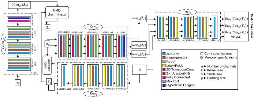
Figure 3: The general architecture of the proposed hybrid model consists of four convolutional networks for the encoder, generator, code generator, and discriminator.

The overall architecture of our model is depicted in Figure 3.

5 Experimental Results

In this section, we present the results of our experiments on four datasets to evaluate the performance of our models. We implement our models using the PyTorch library in Python. We set the mini-batch size to 16 and the number of workers to 64. As the Hyperbolic tangent activation function is used on the last layer of the generator, we scaled all datasets to the range of $-1$ to $1$ to ensure compatibility with the generator outputs. For comparison purposes, we evaluated our model against Semi-BNP MMD GAN (Fazeli-Asl et al., 2023) and AE+GMMN Li et al. (2015). To provide a comprehensive comparison, we also attempted to modify the 3D $\alpha$-WGPGAN settings to the 2D dimension case and included its relevant results.

5.1 Labeled Datasets

To evaluate model performance, we analyzed two handwritten datasets comprising of numbers (MNIST) and letters (EMNIST). MNIST consists of 60,000 handwritten digits, including 10 numbers from 0 to 9 (labels), each with 784 ($28\times 28$) dimensions. This dataset was divided into 50,000 training and 10,000 testing images, and we use the training set to train the network (LeCun, 1998). EMNIST is freely available online and is sourced from Cohen et al. (2017). It contains 372,450 samples of the 26 letters A-Z (labels). Each letter is represented in a $28\times 28$ dimension. We allocate 85% of the samples to the training dataset, and the rest to the testing dataset.

5.1.1 Evaluating Mode collapse

To examine the capability of the model in covering all modes or preventing the mode collapse, we train a convolutional network to predict the label of each generated sample. The structure of this network is provided in Figure 4. If the generator has effectively tackled the issue of the mode collapse, we anticipate having a similar relative frequency for labels in both training and generated datasets, indicating successful training. Plots (a) and (b) in Figure 6 represent the relative frequency of labels in handwritten numbers and letters datasets, respectively.

To train the classifier, we use the cross-entropy loss function and update the network’s weights with the Adam optimizer over 60 epochs. We assess the classifier’s efficacy by presenting the mean of the loss function across all mini-batch testing samples and the percentage of correct classification (accuracy rate) in Figure 5. The figure showcases the classifier’s exceptional accuracy in classifying the dataset.

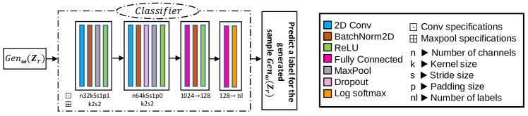
Figure 4: The classifier network architecture for predicting the handwritten dataset’s labels. The output of the fully connected layer is passed through a log softmax function to convert the raw output into a probability distribution over the classes.

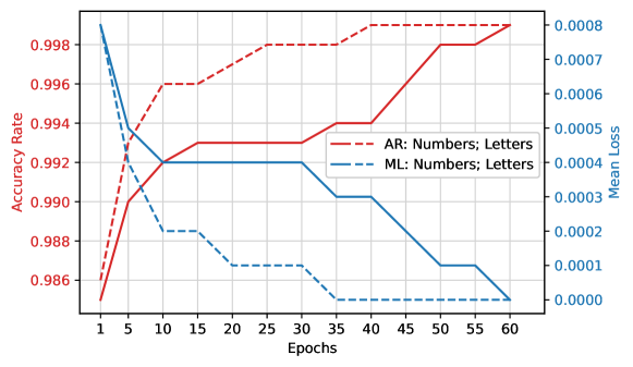
Figure 5: The convolutional classifier’s mean loss (ML) and accuracy rate (AR) with a learning rate of $0.0002$ across all mini-batch testing samples of numbers (solid line) and letters (dashed line) datasets.

The relative frequency plots of predicted labels are depicted in Figure 6, parts (c)-(j), for 1000 generated numbers (left-hand side) and letters (right-hand side) using various generative models. The ratios of the numbers in the training dataset are expected to be consistent, as indicated by plot (a). Examining the plot of generated samples reveals that each model has a distinct bias towards certain digits. Specifically, our model tends to produce digit 6 at a frequency 4.64% higher than that in the training dataset ($14.50\%-9.86\%$), while the semi-BNP MMD GAN exhibits a similar bias towards digit 3 at a 4.18% higher frequency than the training dataset. Nevertheless, these differences are relatively minor compared to AE+GMMN and $\alpha$-WGPGAN, which demonstrate a significant tendency to memorize some modes and overlook certain digits, such as 4 and 8. Similar results can be observed from the relative frequency plots of predicted labels for the letters dataset. Plot (j) in Figure 6 clearly shows the failure of $\alpha$-WGPGAN to maintain the balance of the relative frequency of the data and generate the letter “M”. In contrast, plot (d) indicates that our proposed model successfully preserves the proportion of modes in the generated samples and avoids mode collapse.

5.1.2 Assessing Patterns and Evaluating Model Quality

We employed the principal component analysis (PCA) technique to illustrate the patterns and correlations among data points in a two-dimensional space. Part (a) and (b) in Figure 7 represent the PCA plots for numbers and letters, respectively. Each axis in the plots represents a principal component, with the relevant real dataset used as a reference. It is important to note that PCA provides a necessary condition to verify the similarity pattern between real and fake data distribution. The dissimilarity between PCA plots for real and generated samples indicates that they do not follow the same distribution. However, it is crucial to acknowledge that two similar PCA plots do not necessarily guarantee a similar distribution for real and generated samples. Here, the results presented in Figure 7 demonstrate that all models follow the pattern of the relevant real datasets except for the $\alpha$-WGPGAN in the letters dataset. It obviously indicates a different shape and orientation than the structure of the real dataset.

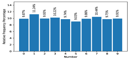
(a) Numbers: Training dataset

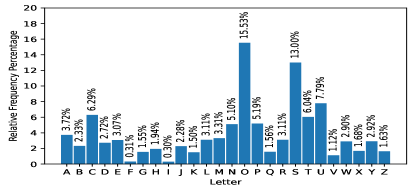
(b) Letters: Training dataset

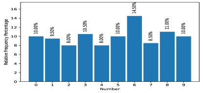
(c) BNP VAE+WMMD

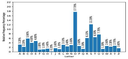
(d) BNP VAE+WMMD

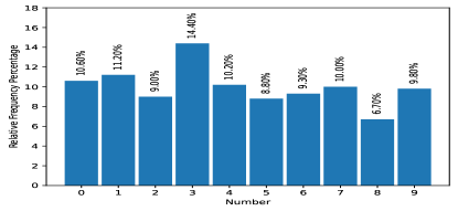
(e) Semi-BNP MMD

(f) Semi-BNP MMD

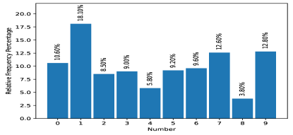
(g) AE+GMMN

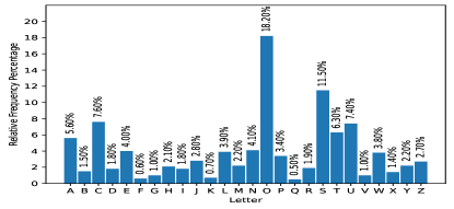
(h) AE+GMMN

(i) $\alpha$-WGPGAN

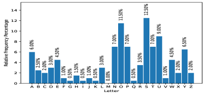
(j) $\alpha$-WGPGAN

Figure 6: The frequency percentage of true and predicted labels for handwritten datasets.

For a more comprehensive analysis, we adopt a mini-batch strategy suggested by Fazeli-Asl et al. (2023) to compute the MMD score, as given by Equation (12), between the generated and real samples. We present the discrepancy scores in density and box plots, along with violin plots in Figure 7, parts (c) and (d). Overall, the MMD scores of all four models suggest some level of convergence around zero. However, the results of the proposed model and the semi-BNP model are comparable, with both models showing better convergence than the other two models. Specifically, part (d) shows our proposed model demonstrates even better convergence than the semi-BNP model, highlighting an improvement of the semi-BNP MMD model by extending it to the VAE+WMMD model.

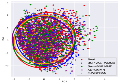
(a) Numbers: PCA plot

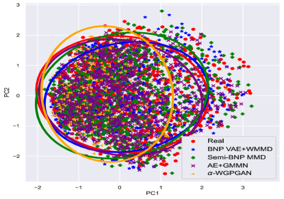
(b) Letters: PCA plot

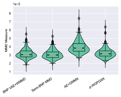
(c) Numbers: Violin plot

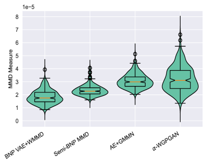
(d) Letters: Violin plot

Figure 7: Top: PCA plots of 1000 generated samples versus real samples with fitted ellipse curves for handwritten datasets, indicating the spread of the samples in the corresponding directions. Bottom: Violin plots of MMD scores including density and box plots.

5.1.3 Visualisation

To better demonstrate the visual capabilities of our proposed model in generating samples, we have displayed 60 samples generated from the model and have compared them to the samples generated by other models, as depicted in Figure 8. While the semi-BNP MMD model displays a range of generated characters in parts (e) and (f) of Figure 8, the images contain some noise that detracts from their quality. On the other hand, the results of AE+GMMN, displayed in parts (g) and (h), reveal blurry outputs that fall short of our desired standards.

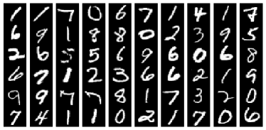
(a) Numbers: Training dataset

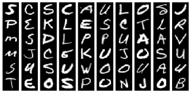
(b) Letters: Training dataset

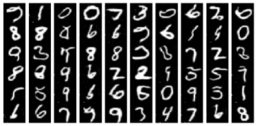
(c) BNP VAE+WMMD

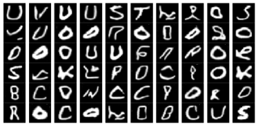
(d) BNP VAE+WMMD

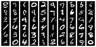
(e) Semi-BNP MMD

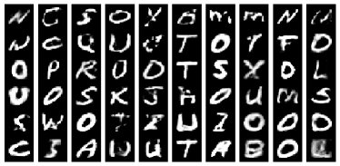
(f) Semi-BNP MMD

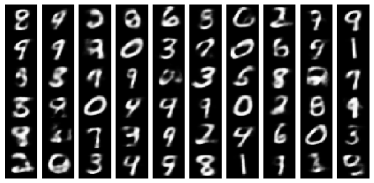
(g) AE+GMMN

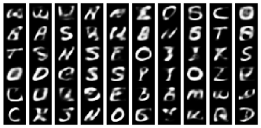
(h) AE+GMMN

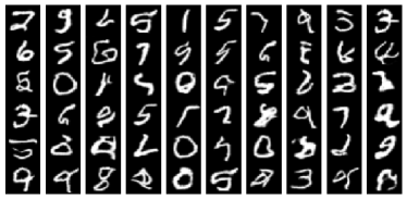
(i) $\alpha$-WGPGAN

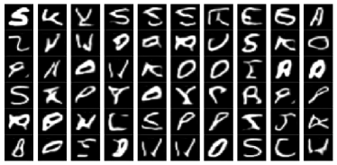
(j) $\alpha$-WGPGAN

Figure 8: Visualisation of handwritten training samples and generated samples using various generative models after 400,000 iterations.

In contrast, the outputs of our model and $\alpha$-WGPGAN exhibit higher-resolution samples without any noise. However, it appears that the generated samples of the $\alpha$-WGPGAN model contain slightly more ambiguous images compared to ours, suggesting that our model converges faster than $\alpha$-WGPGAN.

5.2 Unlabaled Datasets

The performance of a GAN can vary depending on the characteristics of the training dataset, including its complexity, diversity, quality, and size. Thus, it is crucial to assess the model’s effectiveness on more intricate datasets. For a comprehensive evaluation of the model’s performance, facial and medical images are the two most important datasets to consider. In this regard, we use the following two main data sources and resize all images within them to 64$\times 64$ pixels to train all models.

5.2.1 Brain MRI Dataset

The brain MRI images present a complex medical dataset that poses a significant challenge for researchers. These images can be easily accessed online, with both training and testing sets available, comprising a total of 7,023 images of human brain MRI. The dataset includes glioma, meningioma, no tumor, and pituitary tumors (Nickparvar, 2021). The training set is composed of 5,712 images of varying sizes, each with extra margins. To ensure consistency and reduce noise in the training data, a pre-processing code is used to remove margins before feeding them into the networks for training.

Part (a) of Figure 9 illustrates the PCA plots of the generated samples for all models, highlighting that the dispersion and direction of samples generated by $\alpha$-WGPGAN model differ the most from the real dataset compared to the other models. Meanwhile, part (c) of Figure 9 shows almost identical convergence of MMD scores around zero for the compared models. However, Figure 10 portrays noisy and blurry outputs generated by the semi-BNP and AE+GMMN models, whereas our model and the $\alpha$-WGPGAN produce clear outputs.

5.2.2 CelebFaces Attributes Dataset

The CelebFaces attributes dataset (CelebA), collected by Liu et al. (2015), includes 202,599 images of celebrities that are publicly available online. The dataset features people in various poses, with different backgrounds, hairstyles and colors, skin tones, and wearing or not wearing glasses and hats, providing a rich resource for evaluating the performance of data augmentation models.

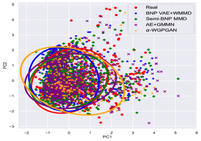
(a) MRI: PCA plot

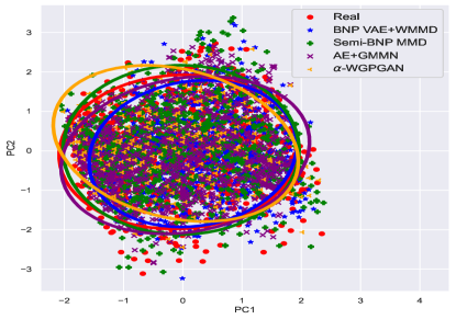
(b) CelebA: PCA plot

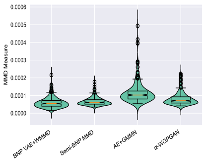
(c) MRI: Violin plot

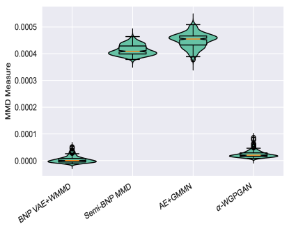
(d) CelebA: Violin plot

Figure 9: Top: PCA plots of 1000 generated samples versus real samples with fitted ellipse curves for MRI and celebA datasets, indicating the spread of the samples in the corresponding directions. Bottom: Violin plots of MMD scores including density and box plots.

While part (b) of Figure 9 shows a slight variation in the direction of the generated sample pattern, part (d) of the same figure highlights a significant gap between the convergence of MMD scores of our proposed approach and $\alpha$-WGPGAN compared to semi-BNP MMD and AE+GMMN around zero. Our proposed model yields even lower MMD scores than $\alpha$-WGPGAN.

On the other hand, despite the limited number of samples shown in Figure 11, the generated images by our proposed model exhibit a remarkable diversity that encompasses a range of hair colors and styles, skin tones, and accessories such as glasses and hats. This variety suggests that our results are comparable to those produced by $\alpha$-WGPGAN. However, it is worth noting that the images generated by the AE+GMMN model not only suffer from blurriness but also appear to be heavily biased toward female faces, indicating a potential issue with mode collapse in this type of dataset. While the samples generated by the semi-BNP MMD model displayed better results than the AE+GMMN, there is still a level of noise present, indicating that more iterations are needed to ensure model convergence.

6 Conclusion

We have proposed a powerful hybrid generative model that has produced realistic samples in the BNP framework. We have extended the semi-BNP MMD GAN, introduced by Fazeli-Asl et al. (2023), by incorporating both Wasserstein and MMD measures into the GAN loss function along with a VAE and an additional code generator to enhance its ability to produce diverse outputs. Different types of datasets have been used to examine the performance of the proposed model, indicating that it is a competitive model. Our model has also been compared to several generative models, such as $\alpha$-WGPGAN, and has outperformed them in terms of mitigating mode collapse and producing noise-free images.

To improve the efficiency and effectiveness of communication between the generator and discriminator networks, we plan to employ multiplex networks in our model. Multiplex networks can tackle the problem of data sparsity in GANs by incorporating multiple types of interactions and relationships between nodes. This allows the model to learn from a larger and more diverse set of data, improving its ability to generate realistic samples. For future work, we are considering extending our proposed idea to include 3D medical datasets for detecting anomalies like Down syndrome in fetuses. This development could prevent the birth of defective babies. We hope that a more powerful generative model can help solve important issues in medical imaging.

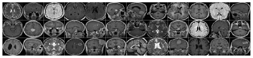
(a) Training dataset

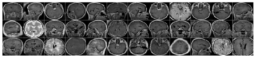
(b) BNP VAE+WMMD

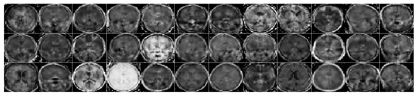
(c) Semi-BNP MMD

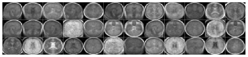
(d) AE+GNNM

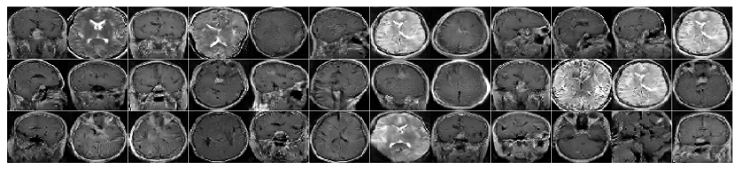
(e) $\alpha$-WGPGAN

Figure 10: Visualisation of MRI training samples and generated samples using various generative models after 400,000 iterations.

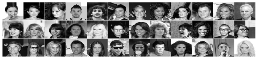
(a) Training dataset

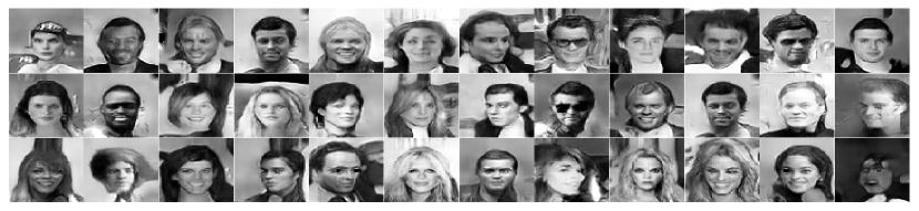
(b) BNP VAE+WMMD

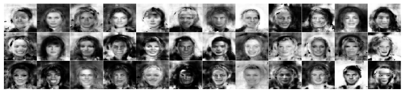
(c) Semi-BNP MMD

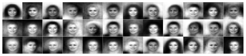
(d) AE+GNNM

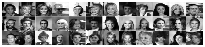
(e) $\alpha$-WGPGAN

Figure 11: Visualisation of celebA training samples and generated samples using various generative models after 400,000 iterations.

References

- Arjovsky and Bottou (2017) M. Arjovsky and L. Bottou. Towards principled methods for training generative adversarial networks. CoRR, abs/1701.04862, 2017. URL http://arxiv.org/abs/1701.04862.
- Arjovsky et al. (2017) M. Arjovsky, S. Chintala, and L. Bottou. Wasserstein generative adversarial networks. In International Conference on Machine Learning, pages 214–223. PMLR, 2017.
- Bondesson (1982) L. Bondesson. On simulation from infinitely divisible distributions. Advances in Applied Probability, 14(4):855–869, 1982.
- Cohen et al. (2017) G. Cohen, S. Afshar, J. Tapson, and A. Van Schaik. EMNIST: Extending MNIST to handwritten letters. In 2017 International Joint Conference on Neural Networks, pages 2921–2926. IEEE, 2017.
- Creswell and Bharath (2018) A. Creswell and A. A. Bharath. Denoising adversarial autoencoders. IEEE Transactions on Neural Networks and Learning Systems, 30(4):968–984, 2018.
- Donahue et al. (2016) J. Donahue, P. Krähenbühl, and T. Darrell. Adversarial feature learning. arXiv preprint arXiv:1605.09782, 2016.
- Dumoulin et al. (2016) V. Dumoulin, I. Belghazi, B. Poole, O. Mastropietro, A. Lamb, M. Arjovsky, and A. Courville. Adversarially learned inference. arXiv preprint arXiv:1606.00704, 2016.
- Dziugaite et al. (2015) G. K. Dziugaite, D. M. Roy, and Z. Ghahramani. Training generative neural networks via maximum mean discrepancy optimization. In Proceedings of the Thirty-First Conference on Uncertainty in Artificial Intelligence, pages 258–267, 2015.
- Evans (2015) M. Evans. Measuring statistical evidence using relative belief. CRC Press, Boca Raton, FL, 2015.
- Fazeli-Asl et al. (2023) F. Fazeli-Asl, M. M. Zhang, and L. Lin. A semi-Bayesian nonparametric hypothesis test using maximum mean discrepancy with applications in generative adversarial networks. arXiv preprint arXiv:2303.02637, 2023.
- Ferguson (1973) T. S. Ferguson. A Bayesian analysis of some nonparametric problems. The Annals of Statistics, 1(2):209–230, 1973.
- Goodfellow et al. (2014) I. Goodfellow, J. Pouget-Abadie, M. Mirza, B. Xu, D. Warde-Farley, S. Ozair, A. Courville, and Y. Bengio. Generative adversarial nets. Advances in Neural Information Processing Systems, 27:2672–2680, 2014.
- Gretton et al. (2012) A. Gretton, K. M. Borgwardt, M. J. Rasch, B. Schölkopf, and A. Smola. A kernel two-sample test. The Journal of Machine Learning Research, 13(1):723–773, 2012.
- Gulrajani et al. (2017) I. Gulrajani, F. Ahmed, M. Arjovsky, V. Dumoulin, and A. C. Courville. Improved training of Wasserstein GANs. Advances in Neural Information Processing Systems, 30, 2017.
- Im et al. (2017) D. Im, S. Ahn, R. Memisevic, and Y. Bengio. Denoising criterion for variational auto-encoding framework. In Proceedings of the AAAI Conference on Artificial Intelligence, volume 31, 2017.