JL-Lemma derived Optimal Projections for Discriminative Dictionary Learning

Abstract

To overcome difficulties in classifying large dimensionality data with a large number of classes, we propose a novel approach called JLSPCADL. This paper uses the Johnson-Lindenstrauss (JL) Lemma to select the dimensionality of a transformed space in which a discriminative dictionary can be learned for signal classification. Rather than reducing dimensionality via random projections, as is often done with JL, we use a projection transformation matrix derived from the proposed Modified Supervised PC Analysis (M-SPCA) with the JL-prescribed dimension. JLSPCADL provides a heuristic to deduce suitable distortion levels and the corresponding Suitable Description Length (SDL) of dictionary atoms to derive an optimal feature space and thus the SDL of dictionary atoms for better classification. Unlike state-of-the-art dimensionality reduction-based dictionary learning methods, a projection transformation matrix derived in a single step from M-SPCA provides maximum feature-label consistency of the transformed space while preserving the cluster structure of the original data. Despite confusing pairs, the dictionary for the transformed space generates discriminative sparse coefficients, with fewer training samples. Experimentation demonstrates that JLSPCADL scales well with an increasing number of classes and dimensionality. Improved label consistency of features due to M-SPCA helps to classify better. Further, the complexity of training a discriminative dictionary is significantly reduced by using SDL. Experimentation on OCR and face recognition datasets shows relatively better classification performance than other supervised dictionary learning algorithms.

[inst1]organization=OCR Lab, School of Computer and Information Sciences,addressline=University of Hyderabad, city=Hyderabad, postcode= 500046, state=Telangana, country=India. [inst2]organization=Visiting Scientist, School of Computer and Information Sciences,addressline=University of Hyderabad, city=Hyderabad, postcode= 500046, state=Telangana, country=India.

1 Introduction

For high-dimensional signal classification, the Sparse Representation (SR) model offers the best method for finding the latent feature space, avoiding hand-crafted feature extraction. With the proposal that the SR model is similar to the receptive field properties of the visual cortex in mammals [31], the use of overcomplete ($\#columns>\#rows$) learned dictionaries [4, 29] in the SR model became popular for richer representations and classification. However, discriminative feature extraction using the SR model with reduced computations requires training a shared dictionary that has low dimensional atoms (columns) with global and local features. Though compact, the dictionary must explain the data well. The Minimum Description Length (MDL) [17] principle asserts that the best model avoiding overfit that explains the data is given by the one with the least number of parameters. An embedding theorem for manifolds [30] proposed by John Nash guarantees that a manifold can be isometrically embedded into a $\mathbb{R}^{p}$ with Euclidean geometry i.e. curves retain their arc-length even after embedding. However, a simple brute-force approach of embedding data into a lower dimensional space may not always give a better separation of data. To reduce the model complexity to avoid model overfit, a robust dimensionality reduction method is required. Though there are several dimensionality reduction methods, they do not guarantee class separation in the transformed space.
While projecting to a lower dimensional space, the number of dimensions is a random choice in conventional dimensionality reduction-based Dictionary Learning (DL) methods. The JL-lemma [21] gives the minimal number of dimensions $p$, required to transform data into a lower dimensional space using gaussian random projections, without exceeding a bounded perturbation of the original geometry. Each $p$ of a dataset depends on the dataset size $N$ and the required data perturbation threshold $\epsilon$. However, such random projections do not guarantee feature label consistency. In this context, we propose a heuristic to determine the suitable data perturbation threshold and the corresponding values of $p$, as a novel practical utility. We call this $p$ the Suitable Description Length (SDL) of dictionary atoms in the transformed space. We also propose Modified-SPCA to derive a constructive projection matrix with $p$ orthonormal principal components and the dictionary learning algorithm JLSPCADL which learns dictionary atoms of SDL size. Unlike Supervised PCA [8] where the number of principal components is randomly chosen, the proposed Modified Supervised PCA (M-SPCA) with suitable number of principal components ($p$) gives the best suitable transformation matrix for each dataset. This transformation is designed to maximize the dependence between the data and the labels, based on Hilbert-Schmidt Independence Criterion (HSIC) [8]. Learning a dictionary with atoms of dimensionality $p$ (SDL) in such transformed space results in discriminative atoms and the corresponding discriminative coefficients could be used as features for better classification performance. If two data points are far from each other in the original space but very close in the transformed space, it is highly likely that these two are coded using the same set of dictionary atoms, leading to misrepresentation and misclassification. M-SPCA avoids such embeddings using the JL-lemma. An argument supporting the Subspace Restricted Isometry Property (RIP) in the proposed M-SPCA-embedded space is given in Section 4 and a detailed proof of the same is given in the Appendix. Subspace RIP guarantees the separation of classes in the projected space.

1.1 Highlights of JLSPCADL

• A heuristic to determine the optimal data distortion threshold and the corresponding interval for optimal dimensionality $p$ based on the JL-lemma is proposed. This optimal dimensionality is the SDL for dictionary atoms.

• A non-iterative constructive approach is given to obtain the optimal transformation matrix when $p\leq d$ and when $p>d$.

• Projected space satisfying JL-lemma implies subspace RIP i.e. the pairwise distances between subspaces are preserved in the transformed space.

• Cluster structure of the original data is preserved in the projected space.

• We achieve maximum feature-label consistency with the proposed projection matrix where the $p$ principal components include label information.

The notation used in this article is given in Table 1.1.

Table 1.1: Notation.

Matrix	$A-Z$
Vector	a-z
$\|.\|_{p}$ or $l_{p}$-norm, $\|\textbf{a}\|_{p}=$	$(\sum\limits_{j=1}^{n}|a_{j}|^{p})^{(1/p)}$
Frobenius norm, $\|A\|_{F}=$	$\sqrt{\sum\limits_{i=1}^{m}\sum\limits_{j=1}^{n}|a_{ij}|^{2}}$
Inverse and Transpose	Superscripts $-1$ and $T$
Identity matrix	$I$
Pdf of a Gaussian multivariate	$\mathcal{N}(X;\mathbf{\mu},\Sigma)$
Trace of matrix $A$	$tr(A)$
No. of samples/class	$\#S_{C}$
No. of iterations	$n$
Projection dimension	$p$

1.2 Sparse Representation Problem

Given a set of $N$ training images $Y=\{\bf{y}_{i},i=1,\ldots,N|$ $\bf{y}_{i}\in\mathbb{R}^{d\times 1}\}$ from $C$ classes, and the corresponding label matrix $H\in\mathbb{R}^{C\times N}$, the problem is to find a dictionary $D\in\mathbb{R}^{d\times K}$ and the corresponding coefficient matrix $X\in\mathbb{R}^{K\times N}$ such that $Y\approx DX+\epsilon$. Using $l_{1}-$norm regularization, the SR optimization problem is

$$<\hat{D},\hat{X}>=\operatorname*{arg\,min}_{D,X}(\|Y-DX\|_{F}^{2}+\lambda\|X\|_{0}).$$ (1.1)

subject to $\|d_{j}\|\leq 1,\forall j=1,2,\ldots,K$, $\|\bf{x}_{j}\|_{0}\leq T,\forall\bf{x}_{j}\in X$ . Here $\hat{D},\hat{X}$ denote the optimal values of $D,X$, and $T$ is called Sparsity threshold. The unit norm constraint on columns of the dictionary avoids arbitrarily large coefficients in $X$. The optimization problem in equation (1.1) can be solved by updating coefficient matrix X w.r.t a fixed dictionary $D$ (called Sparse Coding), and updating $D$ w.r.t a fixed $X$ (called Dictionary Learning, DL).

Table 1.2 presents how different parameters of DL are determined mathematically and statistically.

Table 1.2: Mathematical Determination of Parameters.

Parameter	Determined by
$p$	Using JL-lemma
$\epsilon$	Graph of $\epsilon$ vs $\frac{dp}{d\epsilon}$
$U$	Using SPCA
$K$	$\#S_{C}\times\#Classes$
Sparsity, $T$	M-SBL at convergence

We discuss related work in section 2 and JL-lemma application in section 3, the proposed method for dictionary learning in section 4, classification rule in section 5, experimental results in section 6, discussion and conclusions in Section 7 and Section 8. Detailed proof that the proposed projection matrix transforms data such that the Subspace RIP holds, Modified KSPCA, and its Complexity are explained in the Appendix.

2 DL in reduced dimensionality space: Related work

When the number of classes is high, learning a shared discriminative dictionary along with a classifier [40],[20],[38] becomes computationally viable. Sparse coefficients learned w.r.t. a shared discriminative dictionary are powerful discriminative features for classification as demonstrated in [27]. However, the parameters of the dictionary, i.e., the description length (dimensionality) of atoms, and the number of atoms have to be optimal for reduced complexity and improved performance. Methods imposing low-rank constraints tend to decrease the description length of dictionary atoms. A synthesis-analysis dictionary pair with a low-rank constraint on the synthesis dictionary along with the coefficient matrix are alternatively updated, iteratively until convergence in ERDDPL [32]. To handle noisy (occluded or corrupted) data and large intra-class variations, the low-rank method JPLRDL [13] uses two graph constraints to impose desirable structure on the latent feature space, along with low rank. There have been attempts to first reduce the dimensionality of data and then learn the dictionary in the transformed subspace [36]. It is important to find the correct embedding or projection of data so that the dictionary learned in the transformed space generates useful coefficients as features of data. In Kernelized Supervised DL (KSDL) [14], Supervised PCA (SPCA) has been applied to the training data to get an orthonormal transformation matrix whose transpose is used as the dictionary. Here, the description length of the atoms is reduced to a random number. In [39], a gradient descent-based approach is given for discriminative orthonormal projection of original data into a subspace and simultaneous dictionary learning for Sparse Representation based Classification (SRC [34]). However, the method becomes computationally intensive when there are a large number of classes and might result in suboptimal solutions when the solution space is non-convex. JDDRDL [12] jointly learns projection matrix for reducing dimensionality and learns discriminative dictionary iteratively. SDRDL [37] simultaneously learns the projection matrix for each class and corresponding class-wise dictionaries iteratively. As the number of classes increases, the generation of sparse coefficient of test signal w.r.t each class-specific dictionary consumes time. The above methods try to reduce the dimensionality using an initialization of the projection operator and simultaneously learn the dictionary and coefficients iteratively until convergence. If this initial guess is far from optimal, convergence is delayed due to accumulated error. Instead of iteratively updating the embedding operator, our objective function is designed to find the transformation matrix in a single step. In this work, we propose to use the JL-lemma to determine the number of features required such that the original clusters are preserved. This optimal dimensionality for the projection of a dataset becomes the Suitable Description Length (SDL) of dictionary atoms. The columns of the projection matrix are derived using Modified-SPCA which uses SDL as the number of principal components. Now, the question of whether this projection matrix is a JL-embedding and guarantees Subspace RIP in the transformed space or not remains to be answered.

3 The Johnson-Lindenstrauss Lemma

Reducing the dimensionality before learning the dictionary enables computing with limited resources and avoids model over-fit.

Lemma 3.1.

JL-Lemma [10]: Given a set of $N$ data points in $\mathbb{R}^{d}$ and $0<\epsilon<1$, if $\displaystyle p\geq\frac{12\log N}{\epsilon^{2}(1.5-\epsilon)}$, then there exists a map $\displaystyle f:\mathbb{R}^{d}\to\mathbb{R}^{p}$ such that

$$\|f(x_{i})-f(x_{j})\|_{2}^{2} \leq (1-\epsilon,1+\epsilon)\|x_{i}-x_{j}\|_{2}^{2},$$

$$1 \leq i,j\leq N.$$

A proof of JL-lemma in [10] considers $f$ to be a random matrix with entries independently identically drawn from a Gaussian distribution with mean 0 and variance 1. Such a map is guaranteed to preserve distances in the transformed space up to a scale factor of distances between original pairs with probability at least $\frac{1}{N}$ [10]. In [25], the authors theoretically prove the RIP of Gaussian random matrices when the dimension after projection is based on JL-lemma. However, [9] finds a map $\displaystyle U:\mathbb{R}^{d}\to\mathbb{R}^{p}$ which maps any vector $\bar{y}\in\mathbb{R}^{d}$ to $\displaystyle\frac{U^{T}\bar{y}}{\sqrt{p}}$ with a distortion of atmost $\displaystyle(1\pm\epsilon)$, while projecting the vectors into $\displaystyle\frac{2}{\epsilon^{2}}\log 2N$ dimensions. Attempts to derandomize the projection matrices in [2, 3] try to reduce the number of random bits used to project the data by proposing simple probability distributions to fill the entries of the projection matrix. Though the conditions of orthogonality and normality are not imposed on the columns of the transformation matrix, orthonormality is nearly achieved. In [6], the JL-projection matrix entries are from $\{\pm 1\}$, without any bound on $p$. In [10], Gaussian random projection projecting to a dimensionality of $p\geq\frac{24\log N}{3\epsilon^{2}-2\epsilon^{3}}$ is proved to be a JL-embedding. In [5], a product of two random and a deterministic Hadamard matrix gives Fast JL-transform. Here, we propose to use the lower bound on the JL-embedding dimensionality given in [10] in the map given in [9] i.e. $\bar{y}\to U^{T}\bar{y}/\sqrt{p}$.

4 Proposed method: JLSPCADL

The proposed method starts with calculating the optimal projection dimension $p$. Then the transformation matrix with $p$ principal components is obtained from M-SPCA or M-KSPCA. The shared dictionary and the corresponding discriminative sparse coefficients are learned in the transformed space. The framework of JLSPCADL is given in Fig. 4.1.

Figure 4.1: Framework of proposed JLSPCADL for classification

4.1 Determination of optimal $\epsilon$ and $p$

Let $\displaystyle p:\epsilon\in(0,1)\to\frac{12\log N}{\epsilon^{2}(1.5-\epsilon)}+1$. With $\epsilon=0$ being the singularity of $p$. $\displaystyle\frac{dp}{d\epsilon}=\frac{36\log N(\epsilon-1)}{\epsilon^{3}(1.5-\epsilon)^{2}}$. $\frac{dp}{d\epsilon}\to 0$ as $\epsilon\to 1$ which is outside the domain. Instead of arbitrarily selecting $\epsilon$, we look at the point where $\frac{dp}{d\epsilon}\to 0$. Based on data size, the optimal distortion threshold $\epsilon$ used in JL-lemma is selected as the point where the value of $\frac{dp}{d\epsilon}$ tends to zero. This indicates that the value of $p$ is constant after this point. Fig. 4.2 shows pairs of data points from ten classes on the horizontal axis and the distances between them on the vertical axis. If $\epsilon$ is closer to 1, then the distance between the mapped data points (solid red line ), $\|f(x_{i})-f(x_{j})\|_{2}^{2},\forall i,j$, could blow up as shown in Fig.4.2.

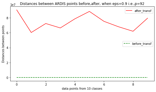
Figure 4.2: Distances between ARDIS points before and after applying PCA with p=92 i.e. when $\epsilon=0.9$

If $\epsilon$ is closer to 0, then the value $p$ increases, which is undesirable. Thus, the optimal distortion threshold interval considered here is $[0.3,0.4]$ and the corresponding $p$ is the optimal projection dimensionality interval. From our experiments, it is found that the value of $p$ beyond this interval gives sub-optimal results either in terms of classification accuracy or computing time, or both. For example, the UHTelPCC dataset has $N=50000$ samples for training. We consider the value of $p$ corresponding to $\epsilon\in[0.3,0.4]$, decreasing from 522 to 320. This implies that $p\geq 320$ for $\epsilon=0.4$, preserves the clusters such that

$$\|f(x_{i})-f(x_{j})\|_{2}^{2}\in(0.6,1.4)\|x_{i}-x_{j}\|_{2}^{2}$$

. For each dataset, we use such $p$ value as the number of principal components in Modified-SPCA to transform data. Fig. 4.3(a) gives lower bounds of projection dimensions of the datasets used for experimentation.

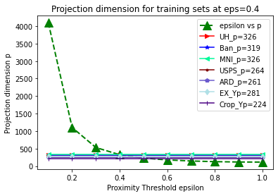
(a) $\epsilon=0.4$

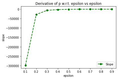
(b) $\epsilon\in{[0.3,0.4]}$

Figure 4.3: (a)Lower bounds on $p$ for $\epsilon=0.4$ (b)$\frac{dp}{d\epsilon}$ vs $\epsilon$. The projection dimension of datasets is chosen at the point where the curve in (b) starts to flatten.

Supervised PCA gives a transformation matrix $U$ based on HSIC criterion [8]. The objective is to find

$$\hat{U}=\operatorname*{arg\,max}_{U}tr(U^{T}YCLCY^{T}U)$$ (4.1)

sub. to $U^{T}U=I$, where $L=HH^{T}$ and $C$ is the data centering matrix. This problem has a closed-form solution from known linear algebra Lemma 4.1.

Lemma 4.1.

If $\hat{U}=\operatorname*{arg\,max}\limits_{U}{tr(U^{T}QU)}$, then the columns of $U$ are the eigenvectors corresponding to the largest p eigenvalues of $Q$.

4.2 Transformation of data using Modified-SPCA (M-SPCA)

Supervised PCA (SPCA) reduces dimensionality while using label information. SPCA gives the least misclassification rates [19] by removing irrelevant dimensions. After scaling the data $Y$ to standard mean and variance, we have M-SPCA which finds the projection matrix with the number of principal components $p$ determined using the JL-lemma as explained in section 4.1. Here, we avoid multiplying with the centering matrix C and thus reduce the complexity. The transformed space $U^{T}Y$ has maximum dependence on the label matrix $H$. Therefore, from HSIC criterion [8], the optimal $U$ is

$$\begin{split}\hat{U}&=\operatorname*{arg\,max}_{U}\{tr((U^{T}Y)^{T}(U^{T}Y)H^{T}H)\}\\ &=\operatorname*{arg\,max}_{U}tr(\underbrace{Y^{T}U}\underbrace{U^{T}YL})\\ &=\operatorname*{arg\,max}_{U}tr(U^{T}\underbrace{YLY^{T}}U).\end{split}$$ (4.2)

sub. to $U^{T}U=I$ where $L=H^{T}H$ is the label kernel matrix. Using Lemma 4.1, we obtain $U$ whose columns are $p$ eigenvectors corresponding to the $p$ largest eigenvalues of $YLY^{T}$. $YLY^{T}$ being a real symmetric matrix has real eigenvalues and the corresponding eigenvectors are orthogonal to each other. Constituting $U_{d\times p},p\leq d$ with a set of orthonormal eigenvectors from these eigenvectors, $U$ is a semi-orthogonal matrix with unit norm columns such that $U^{T}U=I$. From [35], we have the following results on random projection matrices.

Theorem 4.2.

Johnson-Lindenstrauss (JL) Property: A random matrix $A\in\mathbb{R}^{p\times d}$ is said to satisfy JL property if there exists some positive constant $\tilde{c}$ such that for any $0<\epsilon<1$ and for any $\bar{x}\in\mathbb{R}^{d}$, $\displaystyle P(|\|A\bar{x}\|_{2}^{2}-\|\bar{x\|_{2}^{2}}|>\epsilon\|\bar{x}\|_{2}^{2})\leq 2e^{-\tilde{c}\epsilon^{2}p}$.

Lemma 4.3.

Assuming the random matrix $A$ satisfies the JL property, the pairwise distances between the subspaces in the projected space are preserved.

If $A$ is a semi-orthogonal matrix, $\displaystyle\|A\bf{x}\|_{2}^{2}=<A\bf{x},A\bf{x}>=<\bf{x},A^{T}A\bf{x}>=<\bf{x},\bf{x}>=\|\bf{x}\|_{2}^{2}$. Thus, a semi-orthogonal matrix is an isometry. Hence, the proposed projection satisfies the JL property and the resulting space has Subspace RIP. The detailed proof is given in the Appendix.

The objective of JLSPCADL is to find

$$<\hat{U},\hat{D},\hat{X}> = \operatorname*{arg\,min}_{U,D,X}\big{\{}\|U^{T}Y-DX\|_{F}^{2}$$ (4.3)

$$+ \lambda g(X)-tr(U^{T}YLY^{T}U)$$

$$+ \|U^{T}U-I\|_{F}^{2}\big{\}}$$

such that $\|d_{j}\|_{2}^{2}=1\forall j=1,2,\ldots,K$. Here $\lambda$ is a regularization parameter.
The first term in equation (4.3) is the data fidelity term in the transformed space. The second term is a constraint on the coefficients, here sparsity. The third and fourth terms are independent of $D$ and $X$ and hence $U$ can be deduced in a single step using M-SPCA, with the number of principal components $p$ derived above from the JL-lemma. The transformation $U$ contains $p$ PCs of $YLY^{T}$, orthogonal to each other. Thus, $U$ is a semi-orthogonal transformation that preserves distances and angles between data points. As we have scaled data $Y$ to zero mean and unit variance, the matrix $U$ has entries from $(0,1)$. Hence, this transformation using M-SPCA satisfies the condition stated in [10], in order to preserve the distances with probability $>\frac{1}{N}$. After transformation of data $Y$ into $Z=U^{T}Y$, where $Z\in\mathbb{R}^{p\times N}$, then the problem is to find $D,X$ such that

$$Z\approx DX+noise.$$ (4.4)

4.2.1 Dictionary learning in the transformed space

This jointly non-convex problem is solved using the alternating minimization method. Initializing $D$ as a random Gaussian matrix ensures the Restricted Isometry property of $D$ [26], [7], with dictionary size determined as in Table 6.2. K-SVD is used to update dictionary $D$ and SBL to update $X$ using M-SBL [28]. The second term in (4.3) imposes a sparsity constraint on the coefficient matrix. The sparsity of the coefficient matrix is achieved using SBL, with the assumption of additive Gaussian noise [33] in (4.4) with Gaussian prior on coefficient matrix $X$.

We claim that the proposed projection method transforms data so that a structure exists both in the transformed space and the latent feature space of sparse coefficients. This structure in the form of Euclidean distances has been used in several classifications (SVM, k-NN) and clustering (k-means) methods. The existence of such Euclidean geometry in either space as explained in Claim 4.4 ensures that the cluster structure is preserved using JL-lemma for M-SPCA.

Claim 4.4.

The magnitude of the difference between the cosine similarities of projected data and the cosine similarities of corresponding sparse coefficients is bounded.

Proof.

Let $\mathbf{y_{1}}$,$\mathbf{y_{2}}$ be any two points in the $d-$dimensional space. Let $U^{T}(\mathbf{y_{1}})=\mathbf{z_{1}},U^{T}(\mathbf{y_{2}})=\mathbf{z_{2}}\in\mathbb{R}^{p}$ be their projections where $U\in\mathbb{R}^{d\times p}$ is the transformation matrix. Let $\mathbf{x_{1}},\mathbf{x_{2}}\in\mathbb{R}^{K}$ be their sparse coefficients w.r.t dictionary $D\in\mathbb{R}^{p\times K}$ with $K>p$ (since $D$ is an overcomplete shared discriminative dictionary). We consider sparse coefficients learnt w.r.t $D\in\mathbb{R}^{p\times K}$, as high dimensional features $\displaystyle(K>p)$. From [16] it is clear that the projection matrix constituted by the eigenvectors corresponding to the largest $p$ eigenvalues of $YLY^{T}$ transforms data such that $\displaystyle E\bigg{[}{<\frac{\mathbf{z_{1}}}{\|\mathbf{z_{1}}\|},\frac{\mathbf{z_{2}}}{\|\mathbf{z_{2}}\|}>-<\frac{\mathbf{x_{1}}}{\|\mathbf{x_{1}}\|},\frac{\mathbf{x_{2}}}{\|\mathbf{x_{2}}\|}>}\bigg{]}^{2}$ is bounded. If $X$ is a random variable and $E[X^{2}]<\infty$ then $Var[X]<\infty$. Thus, by Chebychev inequality, the difference between the cosine similarities of the projected data points and the cosine similarities of their corresponding sparse coefficients is bounded. ∎

4.3 Convergence

In JLSPCADL, the last two terms of the objective function are independent of $D,X$. A single-step deduction of the transformation matrix $U$ using SPCA under the orthogonality constraint leads to faster convergence. Table 4.1 and Table 4.2 give the complexities of methods compared here.

Table 4.1: Complexity of Computing Z.

Method	Complexity
SPCA, $p\leq d$	$\displaystyle O(pN^{2}+p^{2}N+d^{3}+pdN)$
KSPCA, $p>d$	$\displaystyle O(p^{2}C+pCN+pN^{2}+d^{3}+pdN)$

Table 4.2: Complexity of Learning Dictionary $D$ .

Method	Complexity
SDRDL [37]	$\displaystyle O(nK^{3})+O(ndKN)$
JDDRDL [12]	$\displaystyle O(nK^{3})+O(ndKN)$
LC-KSVD [20]	$\displaystyle O(K^{3})+O(K^{2}N+K^{2}+cKN)$
KSDL[14]	$\displaystyle O(K^{3})+O(dKN)$
JLSPCADL $K>p$	$\displaystyle O(p^{2}K)+O(pKN)$

The space complexity of JLSPCADL is $\displaystyle O(pd+pN+pK)$ for storing the $U,Z,D$ respectively.

5 Proposed Classification Rule

The sparse coefficients obtained from JLSPCADL retain the reconstruction abilities of the K-SVD dictionary and the local features due to SPCA. The sparsity pattern is the same for the same class samples because the set of dictionary atoms representing the group is the same for all of them. Hence these coefficients can be clustered with mean sparse coefficients or medoids of sparse coefficient vectors of each class as cluster centers. The complexity of finding $C$ medoids is $O(C(n-1)^{2})$, where $n$ is the number of samples in each class. Medoid is easy to compute when new data of the same class is added, as the old medoid is swapped with the new data point only if the sum of distances to all the points is minimum for the new data point. Small sample size for supervised training reduces the computation complexity of class-wise medoids of sparse coefficients when new data is added as demonstrated on the Extended YaleB face image dataset in Table 7.1. The classification rule (5.1) depends on both the reconstruction error and the Euclidean distance between $\mathbf{x_{q}}$ and the medoid of sparse coefficients $\bf{m_{c}}$ of each class.

$$label(\bf{q})=\operatorname*{arg\,min}_{c=1,2,\ldots,C}\{\|\mathbf{z_{q}}-D\mathbf{x_{q}}\|_{2}^{2}+\tau\|\mathbf{x_{q}}-\bf{m_{c}}\|_{2}^{2}\},$$ (5.1)

where $\tau$ is the weightage given to the $l_{2}-$norm between $\mathbf{x_{q}}$ and $\bf{m_{c}}$. The framework for discriminative dictionary learning and image classification is described in Algorithm 1.

Algorithm 1 JLSPCADL

1:Input:Normalized data $Y$, $\sigma^{2},\epsilon$

2:Output:label($\bf{q}$

3:Compute $p\geq\frac{12\log N}{\epsilon^{2}(1.5-\epsilon)}$ for optimal $\epsilon$.

4:if $p>d$ then

5:     $V$ from (.9).

6:     $Z\leftarrow V^{T}(\Phi(Y)^{T}\Phi(Y))$, where $\Phi$ is Gaussian kernel.

7:     $D\leftarrow random\_normal\_matrix\in\mathbb{R}^{p\times K}$.

8:     Update $D$ using K-SVD s.t. $Z\approx DX$.

9:     $\displaystyle\bf{\alpha}^{(0)}\leftarrow(1,1,\ldots,1)^{T}$.

10:     $\displaystyle X_{1},X_{2},\ldots,X_{C}\leftarrow M-SBL(Y,D,\sigma^{2})$ using M-SBL [28].

11:     $\bf{m_{c}}\leftarrow KMedoids(X_{j}),j=1,2,\ldots,C$, i.e. ${\displaystyle m_{c}=\arg\min_{y\in{X_{j}}}\sum_{j=1}^{N}d(y,X_{j})}$.

12:     Given a query $\mathbf{q}$, $z_{q}\leftarrow V^{T}(\Phi(Y)\Phi(\mathbf{q})$. Find $\mathbf{x_{q}}$ of $z_{q}$ such that $\displaystyle\mathbf{z_{q}}\approx D{\mathbf{x_{q}}}$ using M-SBL [28].

13:else

14:     $U$ from (4.2).

15:     $\displaystyle Z\leftarrow U^{T}Y$.

16:     Do Steps 5 to 9.

17:     Given a query $\mathbf{q}$, $\displaystyle\mathbf{z_{q}}\leftarrow U^{T}\mathbf{q}$.

18:     Find ${\mathbf{x_{q}}}$ of $\displaystyle\mathbf{z_{q}}$ w.r.t $D$ such that $\displaystyle\mathbf{z_{q}}\approx D{\mathbf{x_{q}}}$ using M-SBL [28].

19:end if

20:Classify using (5.1).

6 Experiments and Results

Datasets and their characteristics are given in Table 6.1. The optimal set of parameters of JLSPCADL for different datasets is given in Table 6.2. The weightage parameter $\tau$ in the classification rule has been empirically set as $0.3$ for Telugu OCR datasets and face recognition datasets while it is set as $0.2$ for handwritten numerals OCR datasets.

Table 6.1: Characteristics of Datasets

Data	$\#C$	$|Maj.class|$	$|Minorclass|$	$Bal.ratio=\frac{|Maj|}{|Minor|}$
UHTelPCC [22]	$325$	4392	20	219.6
Banti[1]	$457$	412	17	24.23
MNIST[11]	10	6742	5421	1.24
USPS[18]	10	1194	542	2.2
ARDIS[23]	10	660	660	1
Ext.YaleB[15]	28	495	445	1.11
Crop.YaleB[24]	38	56	45	1.25

Table 6.2: Optimal parameters of JLSPCADL.

Dataset	$p$ (SDL)	$\#S_{C}$	$K$	T
UHTelPCC	$[320,522]$	20	6500	15
Banti	$[319,520]$	10	4570	8
MNIST	$[326,531]$	25	250	19
USPS(KSPCA)	$[264,430]$	20	200	16
ARDIS	$[261,424]$	20	200	18
YaleB	$[281,457]$	30	840	26
Cropped YaleB	$[224,365]$	30	1140	29

Table 6.3: Results of JLSPCADL on datasets

Data	[20]	[14]	[27]	Our	F1
UHTelPCC	74.6	78.43	99.21	$\bf{99.69\pm 0.78}$	99.43
Banti	65.2	71.9	91	$\bf{91.3\pm 0.34}$	90.92
MNIST	93.6	89.43	98.13	$96.66\pm 0.813$	95.9
USPS	91.2	96.81	94.3	$\bf{97.2\pm 0.56}$	96.1
ARDIS	90.9	90.24	94.12	$\bf{95.6\pm 0.76}$	94.4
Ext. YaleB	84	85	97	$\bf{99.78\pm 0.13}$	99.32
Cropped YaleB	79.8	87	95.9	$95.46\pm 0.89$	94.80

Ten-fold cross-validation results on Telugu OCR datasets have been obtained on an Intel R Xeon(R) CPU E5-2620 v3 @ 2.40GHz processor with 62.8 GiB RAM. A number of samples from each class required for training the dictionary under different transformations versus accuracy on Telugu datasets are depicted in Fig. 6.2. We observe that the misclassification of Telugu printed OCR images is high using LCKSVD where a classifier matrix is learned along with the dictionary. Classification performance of our method on the Telugu dataset UHTelPCC is better, despite confusing pairs (inter-class similarity) as shown in Fig. 6.1. Misclassification of Banti characters could be attributed to different font styles used in the dataset, with high intra-class variability as shown in Fig. 6.1.

Figure 6.1: Inter-class similarity of UHTelPCC data (first row) and Intra-class variance of Banti data (second row)

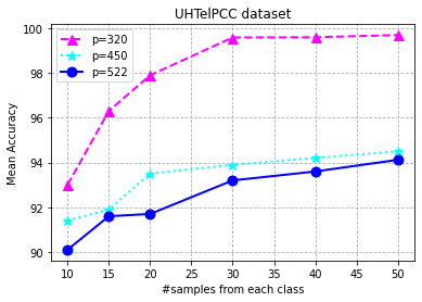
(a) $p=320$ for UHTelPCC ($d=1024$)

(b) $p=319$ for Banti ($d=1024$)

Figure 6.2: Small sample size from each class to form a shared global dictionary versus test accuracy using the proposed method.

Three-fold cross-validation results on handwritten numerals datasets have been performed on Intel(R) Core(TM) i7-10510U CPU @ 1.80GHz x8 processor with 15.3 GiB RAM.

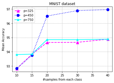
(a) $p=450$ better for MNIST ($d=784$).

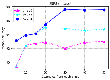
(b) $p=264$ better for USPS ($d=256$).

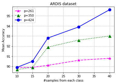
(c) $p=424$ better for ARDIS ($d=784$).

Figure 6.3: Classification accuracy for different projection dimensions on handwritten digit datasets.

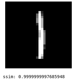
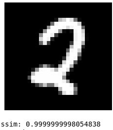
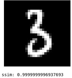
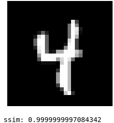
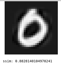
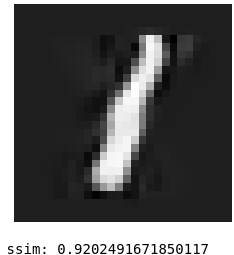
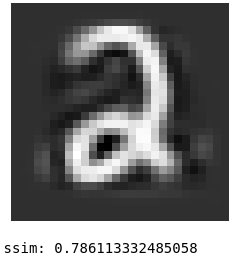
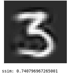
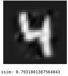
Figure 6.4: Sample reconstructed images with SSIs, of USPS dataset for $p=256$ (with SPCA), w.r.t. the class specific dictionaries (First row) and w.r.t the shared discriminative dictionary (second row).

For face recognition datasets, the optimal distortion threshold interval is decided as $\epsilon\in[0.3,0.4]$ graphically with $p$ decreasing from 457 to 281. We considered $p=950,p=750$, and $p=457$ to observe how the projection dimension and sample size influence the classification accuracy on the Extended YaleB dataset as shown in Fig. 6.5 (a), Fig. 6.5 (b). Though higher dimensions give better accuracy, $p=457$, for $N=13104$ is considered better due to its consistent performance. Similarly, for Cropped YaleB dataset, $p=365$, for $N=1939$ gives a consistent performance. For comparison with other dimensionality reduction-based DL methods as given in Table 7.2, noisy Ext. YaleB with $30\%$ corrupted pixels has been used ( Fig. 6.5(d)).

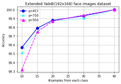
(a) $p=457$ better on
YaleB ($d=192\times 168$)

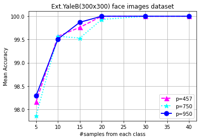
(b) $p=950$ better on
YaleB ($d=300\times 300$)

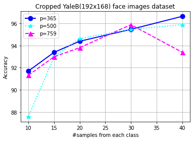
(c) $p=365$ better for cropped YaleB ($d=32256$)

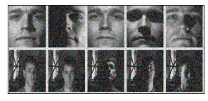
(d) Sample noisy YaleB images

Figure 6.5: Classification performance on YaleB is better when the distortion threshold is low.

For Cropped YaleB dataset, we considered $p=365,p=500$, and $p=759$ to observe how the projection dimension and sample size influence the classification accuracy as shown in Fig. 6.5(c).

7 Discussion

Classification performance has been compared with LCKSVD indicating the improved label consistency of JLSPCADL irrespective of the training sequence and with KSDL to show that a non-orthogonal dictionary learned in the transformed space is better for the classification of the datasets considered here. Unlike the CNN-based methods which require GPUs, the proposed method classifies comparably well with lean computational facilities. The proposed classification rule is able to classify YaleB datasets with results on par with the state of the art. However, the classification of synthetic Telugu OCR dataset Banti with high intra-class variance is inferior to [27]. The results of classification on handwritten numerals are inferior to those of CNN-based methods. The first row of Fig. 6.4 are handwritten numerals from the USPS dataset constructed using class-specific dictionaries learned using K-SVD (SPCA, when $p=256$ ). The second row of Fig. 6.4 corresponds to the images reconstructed using an under-complete (no. of dictionary columns less than dimensions, $p(=264)>d(=256)$) discriminative dictionary, where the reconstruction quality is not good, but the classification is better than LCKSVD and KSDL methods. Training and testing times of JLSPCADL on the Extended YaleB dataset are given in Table 7.1. The decreasing values of training time, when new samples are added, are due to the time saved in computing the medoids of sparse coefficients of each class. The testing times increase slightly due to the increase in the size (number of columns or atoms) of the dictionary. Table 7.2 compares the classification performance of JLSPCADL on $30\%$ corrupted images of Ext. YaleB dataset. It is observed that JLSPCADL is superior when compared to other dimensionality reduction-based methods and low-rank methods. JDDRDL’s and SDRDL’s performance is given on noiseless data.

Table 7.1: Training time on the Ext. YaleB

$\#S_{C}$	$Tr.time$(s)	$Testtime/signal$(ms)
10	359.5	0.3
15	351.6	0.42
20	346.49	0.46
30	340.1	0.47
40	329.4	0.59

Table 7.2: Comparison on the noisy Ext. YaleB

Method	$Tr.time$(s)	Acc.	F1
LCKSVD	320.8	66.71	66.71
ERDDPL	20.08	68.9	68.9
JPLRDL	-	70.1	70.1
SDRDL	-	96.7 w/o noise	96.7
JDDRDLp=450	-	67 w/o noise	67
JLSPCADL	334.8	89.9	89.9

8 Conclusion

Unlike other iterative optimization methods, JLSPCADL, with a single-step method to obtain a transformation matrix for dimensionality reduction, ensures that the distances and the angles between the original data points are preserved after transformation. Sparse coefficients determined using M-SBL w.r.t the global shared dictionary $D$ exclude the irrelevant features. Real-time implementation is possible with small computational facilities, as the transformation of data and dictionary learning is a one-time computation. The experimental results on various types of image datasets show that the proposed approach gives better results in spite of confusing pairs, even in the case of highly imbalanced datasets. Under the proposed framework, a non-parametric approach to learning optimal dictionary size and atoms could be attempted. Replacing Gaussian prior on coefficient vectors with a global-local shrinkage prior leads to correct shrinkage of large signals and noise. We would like to take up these modifications in our future work.

.1 Subspace RIP holds as $U$ satisfies JL property (Theorem 4.2

)

Lemma .1.

The proposed projection matrix $U_{d\times p}=[\hat{e}_{i}]_{i=1}^{p}$ contains $p$ orthonormal eigenvectors of $YLY^{T}$. Any $\bf{y}\in\mathbb{R}^{d}$ is mapped to $\frac{U^{T}\bar{y}}{\sqrt{p}}$ i.e. $\bar{z}=\frac{U^{T}\bar{y}}{\sqrt{p}}$. Then the following conditions hold.
(a) $\displaystyle E[\|\bar{z}\|_{2}^{2}]\leq E[\|\bar{y}\|_{2}^{2}]$
(b) $\displaystyle P(\|\bar{z}\|_{2}^{2}\notin(1\pm\epsilon)\|\bar{y}\|_{2}^{2})\leq 2e^{-\tilde{c}\epsilon^{2}p}$.

Proof.

(a) Using the Cauchy-Schwarz inequality, for any $\bar{y}\neq\bar{0}\in\mathbb{R}^{d}$, we have

$$\begin{split}\frac{\|U^{T}\bar{y}\|_{2}^{2}}{\|\bar{y}\|_{2}^{2}}&\leq\|U^{T}\|_{2}^{2}\end{split}$$ (.1)

$$\begin{split}E[\|\bar{z}\|_{2}^{2}]&=\frac{1}{p}E[\|U^{T}\bar{y}\|_{2}^{2}]\leq\frac{1}{p}E[\|U^{T}\|_{2}^{2}\|\bar{y}\|_{2}^{2}]\leq\frac{1}{p}E[\|U^{T}\|_{F}^{2}\|\bar{y}\|_{2}^{2}]\\ &=\frac{1}{p}E[trace(I_{p})\|\bar{y}\|_{2}^{2}]\\ &=E[\|\bar{y}\|_{2}^{2}]\end{split}$$ (.2)

(b) Using $\log(1-x)=-x-\frac{x^{2}}{2}-\frac{x^{3}}{3}-\ldots$ and

$$\begin{split}\|U\|_{2}\mathrel{\ensurestackMath{\stackon[1pt]{=}{\scriptstyle\Delta}}}\sup_{\bar{w}\neq\bar{0}}\frac{\|U^{T}\bar{w}\|_{2}^{2}}{\|\bar{w}\|_{2}^{2}}=\lambda_{max}\geq\frac{\|U^{T}\bar{y}\|_{2}}{\|\bar{y}\|_{2}}\end{split}$$ (.3)

For any $\bar{y}\neq\bar{0}\in\mathbb{R}^{d}$, we have

$$\begin{split}P(\|\bar{z}\|_{2}^{2}\leq(1-\epsilon)\|\bar{y}\|_{2}^{2})=P(\frac{\|U^{T}\bar{y}\|^{2}}{p}\leq(1-\epsilon)\|\bar{y}\|^{2})\\ =P(e^{-\lambda\frac{\|U^{T}\bar{y}\|_{2}^{2}}{\|\bar{y}\|_{2}^{2}}}\geq e^{-\lambda(1-\epsilon)p})\\ \leq\frac{E[e^{-\lambda\frac{\sum_{j=1}^{p}|z_{j}|_{2}^{2}}{\|\bar{y}\|_{2}^{2}}}]}{e^{-\lambda(1-\epsilon)p}}\end{split}$$ (.4)

Let $t_{j}=\frac{|z_{j}|}{\|\bar{y}\|}$. $\forall\bar{y}\in\mathbb{R}^{d},\frac{\|U^{T}\bar{y}\|}{\|\bar{y}\|}\leq\|U\|_{2}=\lambda_{max}$. According to the Central Limit Theorem, $t_{j}\sim\mathcal{N}(\mu_{j},\sigma_{j}),j=1,2,\ldots,p$. Without loss of generality, let $t_{1j}=\frac{t_{j}-\mu}{\sigma}\sim\mathcal{N}(0,1)$.

$$E[e^{-\lambda t_{1j}^{2}}]=\int_{-\infty}^{+\infty}e^{-\lambda t_{1j}^{2}}\frac{e^{\frac{-t_{1j}^{2}}{2}}}{\sqrt{2\pi}}dt_{1j}$$ (.5)

Therefore,

$$P(\|\bar{z}\|_{2}^{2}\leq(1-\epsilon)\|\bar{y}\|_{2}^{2})\leq\frac{\prod_{j=1}^{p}E[e^{-\lambda t_{1j}^{2}}]}{e^{-\lambda(1-\epsilon)p}}\\ =\frac{1}{(\sqrt{1+2\lambda})^{p}e^{-\lambda(1-\epsilon)p}}$$ (.6)

Choose $\lambda=\frac{\epsilon}{2(1-\epsilon)}>0$ for $0<\epsilon<1$.Therefore,

$$\begin{split}P(\|\bar{z}\|_{2}^{2}\leq(1-\epsilon)\|\bar{y}\|_{2}^{2})&=\frac{(\sqrt{1-\epsilon})^{p}}{e^{-\epsilon p/2}}=((1-\epsilon)e^{\epsilon})^{\frac{p}{2}}\\ &<(e^{-\epsilon-\frac{\epsilon^{2}}{2}}e^{\epsilon})^{\frac{p}{2}}=e^{-\epsilon^{2}p/4}\\ &=e^{-\tilde{c}\epsilon^{2}p},\end{split}$$ (.7)

where $\tilde{c}=\frac{1}{4}>0$.

Similarly, choose $\displaystyle 0<\lambda=\frac{\epsilon}{2(1+\epsilon)}<\frac{1}{2}$ to get

$$\begin{split}P(\|\bar{z}\|_{2}^{2}\geq(1+\epsilon)\|\bar{y}\|_{2}^{2})&\leq\frac{(1+\epsilon)^{\frac{p}{2}}}{e^{\frac{p\epsilon}{2}}}<\frac{(e^{(\epsilon-\frac{\epsilon^{2}}{2})})^{\frac{p}{2}}}{e^{\frac{p\epsilon}{2}}}\\ &=e^{-\frac{p\epsilon^{2}}{4}}\\ &=e^{-\tilde{c}\epsilon^{2}p},\end{split}$$ (.8)

where $\tilde{c}=\frac{1}{4}$ Thus, for any $\bar{y}\in\mathbb{R}^{d}$ $\displaystyle P(\big{|}\|U^{T}\bar{y}\|_{2}^{2}-\|\bar{y}\|_{2}^{2}\big{|}>\epsilon\|\bar{y}\|_{2}^{2})\leq 2e^{-\tilde{c}\epsilon^{2}p}$. Hence, as stated in [35], subspace RIP holds in the transformed space using the proposed projection matrix. ∎

.2 Kernel SPCA

When $p>d,$ Kernel SPCA [8] has been used. The transformation matrix $U$ is expressed as a linear combination of the projected data points. Let $\Phi:$ y $\to$ $feature\_space$, then $U=\Phi(Y)V$. The objective is to find $U$ which maximizes the dependence between $\Phi(Y)$ and the label matrix $H$. After rearranging as in (4.2),

$$\begin{split}\hat{U}=\operatorname*{arg\,max}_{U}\{tr(U^{T}\Phi(Y)H^{T}H\Phi(Y)^{T}U)\}\\ =\operatorname*{arg\,max}_{V}\{tr(V^{T}\Phi(Y)^{T}\Phi(Y)H^{T}\Phi(Y)^{T}\Phi(Y)V)\}\\ =\operatorname*{arg\,max}_{V}\{tr(V^{T}K_{1}H^{T}HK_{1}V)\},\end{split}$$ (.9)

sub. to $U^{T}U=I$ $\implies$ $\displaystyle V^{T}K_{1}V=I$ where $K_{1}=\Phi(Y)^{T}\Phi(Y)$. $\Phi(Y)V$ is a semi-orthogonal matrix and hence is an isometry. The generalized eigenvector problem is solved to get $V=$ $p$ eigenvectors corresponding to the top $p$ eigenvalues of $\displaystyle[K_{1}H^{T}HK_{1},K_{1}]$. The transformed space is given by $Z=(\Phi(Y)V)^{T}\Phi(Y)$ i.e. $\displaystyle Z=V^{T}K_{1}$ whose complexity is $\displaystyle O(Np^{2}+pN^{2})$. $\displaystyle Z_{test}=V^{T}\Phi(Y)^{T}\Phi(y_{test})$.

In the dual formulation problem, find SVD of $\Phi(Y)H^{T}=U\Sigma V^{T}$ and the left-singular vectors of $\Phi(Y)H$ are eigenvectors of $\Phi(Y)HH^{T}(\Phi(Y))^{T}$. In SVD, the first $p$ columns in $U$ corresponding to the first $p$ non-zero singular values are in a one-to-one correspondence with the first $p$ rows of $V^{T}$. Thus, we can reduce $U,\Sigma,V^{T}$ to $U^{1},\Sigma^{1},(V^{1})^{T}$ to get the same result. $U^{1}=\Phi(Y)HV^{1}(\Sigma^{1})^{-1}$ and $Z=(U^{1})^{T}\Phi(Y)\implies$ $Z=(\Sigma^{1})^{-1}(V^{1})^{T}H^{T}\Phi(Y)^{T}\Phi(Y)$. So, the complexity is $O(p^{2}C+pCN+pN^{2})$ where $C$ is the number of classes.

Acknowledgements

The authors would like to thank Dr. Sumohana S.Channappayya for relevant suggestions to improve the article.

References

- [1] Rakesh Achanta and Trevor Hastie. Telugu ocr framework using deep learning. arXiv preprint arXiv:1509.05962.
- [2] Dimitris Achlioptas. Database-friendly random projections. In Proceedings of the twentieth ACM SIGMOD-SIGACT-SIGART symposium on Principles of database systems, pages 274–281, 2001.
- [3] Dimitris Achlioptas. Database-friendly random projections: Johnson-lindenstrauss with binary coins. Journal of Computer and System Sciences, 66(4):671–687, 2003. Special Issue on PODS 2001.
- [4] M. Aharon, M. Elad, and A. Bruckstein. -svd: An algorithm for designing overcomplete dictionaries for sparse representation. IEEE Transactions on Signal Processing, 54(11):4311–4322, Nov 2006.
- [5] Nir Ailon and Bernard Chazelle. Approximate nearest neighbors and the fast johnson-lindenstrauss transform. In Proceedings of the thirty-eighth annual ACM symposium on Theory of computing, pages 557–563, 2006.
- [6] Rosa I Arriaga and Santosh Vempala. An algorithmic theory of learning: Robust concepts and random projection. Machine learning, 63:161–182, 2006.
- [7] Richard Baraniuk, Mark Davenport, Ronald DeVore, and Michael Wakin. A simple proof of the restricted isometry property for random matrices. Constructive Approximation, 28(3):253–263, 2008.
- [8] Elnaz Barshan, Ali Ghodsi, Zohreh Azimifar, and Mansoor Zolghadri Jahromi. Supervised principal component analysis: Visualization, classification and regression on subspaces and submanifolds. Pattern Recognition, 44(7):1357–1371, 2011.
- [9] Ankur Bhargava and S Rao Kosaraju. Derandomization of dimensionality reduction and sdp based algorithms. In Algorithms and Data Structures: 9th International Workshop, WADS 2005, Waterloo, Canada, August 15-17, 2005. Proceedings 9, pages 396–408. Springer, 2005.
- [10] Sanjoy Dasgupta and Anupam Gupta. An elementary proof of a theorem of johnson and lindenstrauss. Random Structures & Algorithms, 22(1):60–65, 2003.
- [11] Li Deng. The mnist database of handwritten digit images for machine learning research [best of the web]. IEEE signal processing magazine, 29(6):141–142, 2012.
- [12] Zhizhao Feng, Meng Yang, Lei Zhang, Yan Liu, and David Zhang. Joint discriminative dimensionality reduction and dictionary learning for face recognition. Pattern Recognition, 46(8):2134–2143, 2013.
- [13] Homa Foroughi, Nilanjan Ray, and Hong Zhang. Object classification with joint projection and low-rank dictionary learning. IEEE Transactions on Image Processing, 27(2):806–821, 2018.
- [14] Mehrdad J. Gangeh, Ali Ghodsi, and Mohamed S. Kamel. Kernelized supervised dictionary learning. IEEE Transactions on Signal Processing, 61(19):4753–4767, 2013.
- [15] A.S. Georghiades, P.N. Belhumeur, and D.J. Kriegman. From few to many: Illumination cone models for face recognition under variable lighting and pose. IEEE Trans. Pattern Anal. Mach. Intelligence, 23(6):643–660, 2001.
- [16] Ioannis Gkioulekas and Todd Zickler. Dimensionality reduction using the sparse linear model. Advances in neural information processing systems, 24, 2011.
- [17] Mark H Hansen and Bin Yu. Model selection and the principle of minimum description length. Journal of the American Statistical Association, 96(454):746–774, 2001.
- [18] Jonathan J. Hull. A database for handwritten text recognition research. IEEE Transactions on pattern analysis and machine intelligence, 16(5):550–554, 1994.
- [19] Xudong Jiang. Linear subspace learning-based dimensionality reduction. IEEE Signal Processing Magazine, 28(2):16–26, 2011.
- [20] Z. Jiang, Z. Lin, and L. S. Davis. Label Consistent K-SVD: Learning a Discriminative Dictionary for Recognition. IEEE Transactions on Pattern Analysis and Machine Intelligence, 35(11):2651–2664, 2013.
- [21] William B Johnson. Extensions of lipschitz mappings into a hilbert space. Contemp. Math., 26:189–206, 1984.
- [22] Rakesh Kummari and Chakravarthy Bhagvati. UHTelPCC: A Dataset for Telugu Printed Character Recognition. In Recent Trends on Image Processing and Pattern Recognition, volume 862, pages 1–13, Dec 2018.
- [23] Hüseyin Kusetogullari, Amir Yavariabdi, Abbas Cheddad, Håkan Grahn, and Hall Johan. Ardis: a swedish historical handwritten digit dataset. Neural computing & applications (Print), 32(21):16505–16518, 2020.
- [24] K.C. Lee, J. Ho, and D. Kriegman. Acquiring linear subspaces for face recognition under variable lighting. IEEE Trans. Pattern Anal. Mach. Intelligence, 27(5):684–698, 2005.
- [25] Gen Li and Yuantao Gu. Restricted isometry property of gaussian random projection for finite set of subspaces. IEEE Transactions on Signal Processing, 66(7):1705–1720, 2018.
- [26] Gen Li, Qinghua Liu, and Yuantao Gu. Rigorous restricted isometry property of low-dimensional subspaces. Applied and Computational Harmonic Analysis, 49(2):608–635, 2020.
- [27] G. Madhuri, Modali N. L. Kashyap, and Atul Negi. Telugu ocr using dictionary learning and multi-layer perceptrons. In 2019 International Conference on Computing, Power and Communication Technologies (GUCON), pages 904–909, 2019.
- [28] G Madhuri and Atul Negi. Discriminative dictionary learning based on statistical methods. In Statistical Modeling in Machine Learning, pages 55–77. Elsevier, 2023.
- [29] Julien Mairal, Francis Bach, Jean Ponce, Guillermo Sapiro, and Andrew Zisserman. Supervised dictionary learning. In Proceedings of the 21st International Conference on Neural Information Processing Systems, NIPS’08, pages 1033–1040, USA, 2008. Curran Associates Inc.
- [30] John Nash. The imbedding problem for riemannian manifolds. Annals of mathematics, pages 20–63, 1956.
- [31] B A Olshausen and D J Field. Natural image statistics and efficient coding. Network: Computation in Neural Systems, 7(2):333–339, 1996. PMID: 16754394.
- [32] Yuxi Wang, Haishun Du, Yonghao Zhang, and Yanyu Zhang. Efficient and robust discriminant dictionary pair learning for pattern classification. Digital Signal Processing, 118:103227, 2021.
- [33] Oliver Williams, Andrew Blake, and Roberto Cipolla. Sparse bayesian learning for efficient visual tracking. IEEE Transactions on Pattern Analysis and Machine Intelligence, 27(8):1292–1304, 2005.
- [34] J. Wright, A. Y. Yang, A. Ganesh, S. S. Sastry, and Y. Ma. Robust face recognition via sparse representation. IEEE Transactions on Pattern Analysis and Machine Intelligence, 31(2):210–227, Feb 2009.
- [35] Xingyu Xu, Gen Li, and Yuantao Gu. Unraveling the veil of subspace rip through near-isometry on subspaces. IEEE Transactions on Signal Processing, 68:3117–3131, 2020.
- [36] Jiexi Yan, Cheng Deng, and Xianglong Liu. Dictionary learning in optimal metric space. Proceedings of the AAAI Conference on Artificial Intelligence, 32(1), Apr. 2018.
- [37] Bao-Qing Yang, Chao-Chen Gu, Kai-Jie Wu, Tao Zhang, and Xin-Ping Guan. Simultaneous dimensionality reduction and dictionary learning for sparse representation based classification. Multimedia Tools and Applications, 76(6):8969–8990, 2017.
- [38] Meng Yang, Lei Zhang, Xiangchu Feng, and David Zhang. Fisher discrimination dictionary learning for sparse representation. 2011 International Conference on Computer Vision, pages 543–550, 2011.
- [39] Haichao Zhang, Yanning Zhang, and Thomas S. Huang. Simultaneous discriminative projection and dictionary learning for sparse representation based classification. Pattern Recognition, 46(1):346–354, 2013.
- [40] Q. Zhang and B. Li. Discriminative k-svd for dictionary learning in face recognition. In 2010 IEEE Computer Society Conference on Computer Vision and Pattern Recognition, pages 2691–2698, June 2010.