Patch-Grid: An Efficient and Feature-Preserving Neural Implicit Surface Representation

Abstract.

Neural implicit representations are increasingly used to depict 3D shapes owing to their inherent smoothness and compactness, contrasting with traditional discrete representations. Yet, the multilayer perceptron (MLP) based neural representation, because of its smooth nature, rounds sharp corners or edges, rendering it unsuitable for representing objects with sharp features like CAD models. Moreover, neural implicit representations need long training time and struggle to represent surfaces with open boundaries. While previous works address these issues separately, we present a unified neural implicit representation called Patch-Grid, which fits to complex shapes efficiently, preserves sharp features delineating different patches and can also represent surfaces with open boundaries and thin geometric features. The efficiency of Patch-Grid comes from encoding each patch with a local grid of spatial latent codes and adaptive resolution, called the patch feature volume, coupled with an MLP decoder mapping grid features to implicit function values. The MLP decoder is shared among all the patch feature volumes and pretrained on a broad variety of local surface geometries; given the pretrained and fixed MLP decoder, novel shapes and local updates can be fitted efficiently by optimizing the patch feature volumes with high flexibility and locality. The faithful preservation by Patch-Grid of sharp edges and corners is enabled by constructive solid geometry (CSG) combinations of patches. To merge the patches with robust CSG operations to produce sharp features, we propose a merge grid that embeds the different patch grids in a common octree structure, and forms CSG combinations locally to achieve better robustness than using a global CSG construction.

Experiments show that our Patch-Grid representation accurately captures shapes with complex sharp features, open boundaries and thin geometric features, and outperforms existing learning-based methods in efficiency for surface fitting and local shape updates.

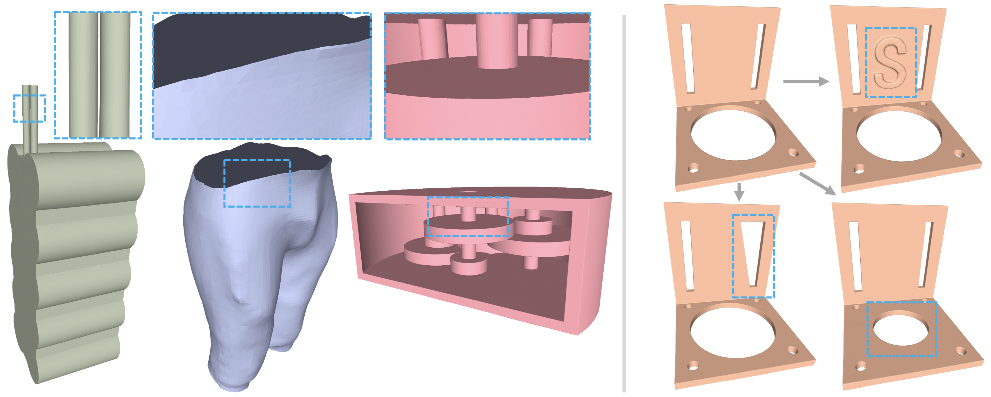
Figure 1. Our Patch-Grid method is capable of (a) modeling diverse geometric features, such as thin geometric features, open surface boundaries, and sharp features (from left to right); (b) Patch-Grid also allows updating a thus learned implicit representation to incorporate bump textures (top right) or reshape a geometric feature (bottom) within 1 second.

A set of models represented by our neural implicit representation.

1. Introduction

The implicit surface representation typically defines a shape as the zero-level set of some function, such as the signed distance function of the shape. The implicit representation is widely used for shape modeling (Turk and O’brien, 2002; Ohtake et al., 2005; Mitchell et al., 2015) and downstream engineering applications like simulation (Allen, 2021). Recent years have seen a surge in research on neural implicit representations (Park et al., 2019; Gropp et al., 2020; Tancik et al., 2020b; Martel et al., 2021) where a deep neural network is used to encode the implicit function in question. Neural implicit representations are inherently smooth and can represent complex shape details more compactly than traditional discrete representations, e.g. point clouds and polygonal meshes (Sitzmann et al., 2020b; Takikawa et al., 2021).

There are two main challenges with current neural implicit surface representations. First, they struggle to represent a variety of geometric features, such as sharp geometric edges, surfaces with open boundaries, and surfaces whose parts form narrow gaps; see some examples in Fig. 1. While there have been some recent attempts to address individual challenges, such as merging a set of neural half-spaces to model sharp geometric edges (Guo et al., 2022) or additionally predicting a mask for extracting open surface boundaries (Chen et al., 2022), there is no unified framework capable of faithfully representing these geometric features in shape modeling.

Second, learning a neural implicit representation to accurately fit a given shape often takes excessively long time, from minutes to around an hour, precluding its application to interactive design. While modern hardware and algorithmic improvement have been proposed to substantially reduce the training time of neural implicit representations (Müller et al., 2022), there is still a demand for faster methods to efficiently model neural implicit surfaces and update existing ones by interactive editing.

To tackle these two challenges, we present Patch-Grid, a compositional framework for modeling neural implicit surfaces with two distinctive advantages: 1) Versatile representation: it can represent sharp geometric features, open surface boundaries, and thin geometric features (such as slender tubes or narrow gaps), which are challenging or impossible for current neural surface representations, as shown in Fig. 1; 2) Superior efficiency: Patch-Grid is faster to train than current neural representations. It typically takes about 8 seconds to train Patch-Grid to fit a given shape and about 1 second to complete a local shape update of an existing surface represented by Patch-Grid. This enables interactive editing of neural implicit surfaces.

The problem we address is formulated as follows. Given a boundary representation (B-Rep) of a 3D shape, which defines the 3D surface shape as a set of surface patches, we aim to convert this B-rep representation into a neural implicit representation, by representing each surface patch as a zero-level set of a neural implicit function. Specifically, each surface patch is tightly contained in a truncated volume that comprises a regular grid of cubic cells with a learnable feature vector assigned to each grid point.

The collection of these grid cells is referred to as the patch volume and the collection of feature vectors defined on it is referred to as the patch feature volume of the surface patch. For any point $\mathbf{x}$ inside a cubic cell, a 3-layered MLP (Multi-Layer Perceptron) decoder is used to map the feature vector at $\mathbf{x}$, which is obtained via trilinear interpolation from feature vectors at the corners of the cell, to a signed distance value, as shown in Fig. 2.

We observe that the global CSG approach adopted by NH-Rep (Guo et al., 2022) for the same task often leads to failure cases in highly concave and narrow regions because multiple surface patches need to be carefully merged in a global manner to avoid undesired interference (cf. Fig. 4). Since the intersection of two or more surface patches forming a sharp geometric feature (edges or corners) is only a local operation, we propose to use a merge grid for robustly modeling sharp features of a given shape in a local manner. Specifically, the merge grid uses an octree structure to adaptively subdivide the spatial domain into cubic cells so that each leaf cell ideally contains no more than one sharp feature to simplify the task. Therefore, our approach circumvents the difficulty in merging multiple patches into various sharp features globally (Guo et al., 2022) by adopting a divide-and-conquer strategy for merging multiple patches in a local region, thereby achieving robust and superior performance for modeling various geometric features as shown in Fig. 1.

Besides sharp features, our local approach is also capable of modeling thin geometric features and open surface boundaries. In a general sense, a slender tube or a narrow gap/slit is considered a thin geometric feature (e.g. columns 1,2,4 in Fig. 15). By adopting a local approach, Patch-Grid robustly models thin geometric features by placing spatially proximal but disjoint surface patches in different patch volumes which may overlap. In this way, the distance fields induced by the different surface patches do not interfere with each other, thereby enabling the modeling of narrow gaps or thin solids formed by these surface patches. Furthermore, we model a boundary curve of an open surface patch as a result of the trimming operation. Therefore, modeling a boundary curve amounts to constructing a trimming surface followed by a trimming operation, which can be performed locally to produce accurate results.

Efficiency. Even without using a sophisticated CUDA implementation, the proposed approach that uses patch-level feature vectors and a merge grid for modeling geometric features can achieve high training efficiency. Typically, our method takes about 8 secs to fit a given shape from scratch and supports local shape updates at an interactive rate (about $\sim$ 1 sec). We will release our code.

In summary, the contributions of this paper are:

• Versatile representation. We present Patch-Grid, a compositional neural implicit representation capable of modeling a variety of geometric features, such as sharp or thin geometric features and open boundaries, that are challenging for previous methods;

• Robustness. A novel merge grid is proposed that adaptively partitions the spatial domain and locally composes neural implicit surface patches to faithfully model a target surface shape with sharp features (i.e. edges and corners) in a more robust manner than the existing global approach (2022).

• Superior efficiency. We present an efficient implementation of Patch-Grid which consists of 1) an adaptive patch feature volume and 2) a merge octree to simplify the merge constraints. Combined with a pretraining strategy, this allows Patch-Grid to achieve a very fast training time (in several seconds) and support local shape updates at an interactive rate ($\sim$ 1 sec), which is much faster than all the existing methods for modeling neural implicit surfaces.

\begin{overpic}[width=433.62pt]{figures/pipeline.png} \put(5.0,32.0){(a) Input shape} \put(26.0,32.0){(b) {Patch-Grid} representation} \put(23.0,29.0){{Patch feature volumes $FV$}} \put(23.0,14.0){{Merge grid $\mathcal{G}$}} \put(46.0,12.0){$f$} \put(50.0,17.0){$\mathcal{L}_{\mathrm{patch}}$} \put(50.0,7.5){$\mathcal{L}_{\mathrm{merge}}$} \put(73.0,8.0){Composition} \put(56.0,32.0){(c) Individual patches} \put(80.0,32.0){(d) Composed result} \end{overpic}

Figure 2. Overview of the proposed Patch-Grid representation. (a) Input to our method is a B-rep model of a 3D shape $\mathcal{S}$; (b) Patch-Grid bounds each surface patch of the given shape with a patch volume. We assign a learnable feature vector $\mathbf{v}_{i}$ to each corner point of the patch volume and convert this volume into a patch feature volume $FV$, which defines a continuous feature field $F(\mathbf{x})$ via trilinear interpolation within each cubic cell. Then, a shared MLP decoder $f$ is used to map $F(\mathbf{x})$ to represent the SDF of the target surface patch. To merge the individual patches together, we construct a merge grid $\mathcal{G}$ and enforce a merge loss within each of the merge grid cells; (c) We design two types of loss terms to enable accurate fitting of individual patches ($\mathcal{L}_{\mathrm{patch}}$) and model the relationship between connected patches ($\mathcal{L}_{\mathrm{merge}}$), respectively; (d) Finally, the individual neural surface patches are composed into the final surface shape that reconstructs the target shape. It takes 8 secs to fit this example.

2. Related works

2.1. Global implicit representation

Neural implicit representation is a novel approach that turns traditional explicit discrete representations (e.g. point clouds, polygon meshes, or voxels) into the iso-surface of some continuously defined differentiable fields represented through a neural network (Park et al., 2019; Mescheder et al., 2019; Chen and Zhang, 2019). To improve the performance when overfitting the network to complex 3D shapes, a series of techniques have been proposed, such as exploring the optimal hyper-parameters (Davies et al., 2020), training strategies (Duan et al., 2020), positional encoding (Tancik et al., 2020a), and sinusoidal activation (Sitzmann et al., 2020b). Another line of work focuses on extending the capability of neural implicit representations to general shapes like open surfaces, such as neural unsigned distance field (Chibane et al., 2020), or modified SDF (Chen et al., 2022). However, these prior approaches cannot faithfully recover sharp features or cannot scale between fine-grained shapes and large scenes.

2.2. Grid- or Patch-based implicit representation

A direct improvement on standard, global, implicit representation is to build spatial grids (Jiang et al., 2020) or octrees (Takikawa2021NGLOD) to split the original shape fitting problem into a set of subproblems. However, due to the grid-based representation strategy, the surface between grids may not be smoothly connected.

Representing the entire shape using a set of shape primitives is a classic point of view in traditional explicit geometry processing (Schnabel et al., 2007; Li et al., 2011; Nan and Wonka, 2017). Those patch-wise representations decompose complex models into multiple patches with parametric shape priors to extract high-level shape structures for downstream applications like shape completion or semantic editing. Motivated by the simplicity of patches, neural implicit representations adopted similar ideas to decompose shapes, allowing learning of locally controllable models (Genova et al., 2020), generalizable parts (Tretschk et al., 2020), or a semantic compositional parametric model (Zhang et al., 2022). However, it is not easy to achieve high representation accuracy by using patch-based implicit representations, due to the difficulty in stitching together or trimming patches.

Focusing on neural implicit modeling of CAD shapes with sharp features, Guo et al. (2022) give a global CSG-based solid entity representation that is based on patch-wise halfspaces. They first propose a top-down constructive method to build the global CSG tree that ensures the order of Boolean operations yields theoretically sound results. Then they supervise learning patch-wise halfspace-based representations on all sample points in the domain, thus coordinating them in the whole space. As we will show in experiments, in contrast to our local approach to CSG construction for sharp feature modeling, the global approach has difficulty precisely representing complex shapes with many concave patches. Moreover, our approach handles more general surface types than solid CAD shapes, including open surfaces, self-intersecting surfaces, and non-orientable surfaces.

3. Our method

3.1. Overview

We present the overview pipeline of Patch-Grid in Fig. 2. Input to our method is a shape $\mathcal{S}=\bigcup_{p=1}^{K}S_{p}$ composed of a collection of surface patches $S_{p}$ along with the type of connection between adjacent patches. Our goal is to represent the shape $\mathcal{S}$ as a neural implicit surface $\mathcal{Z}$ composed of a collection of neural signed distance fields. We denote the zero-level set of a neural signed distance field as $Z_{p}$ which contains a target surface patch $S_{p}$. To facilitate fast training and effective modeling, we introduce a patch volume for each surface patch $S_{p}$ to tightly bound $S_{p}$ and define the extent of $Z_{p}$ as shown in Fig. 2(b). Furthermore, we impose a regular grid structure on the patch volume of $S_{p}$ and assign a feature vector at each grid point. Then the collection of all these feature vectors is referred to as the patch feature volume. Here, the grid resolution is determined by the local shape complexity, as to be explained later. The use of the patch feature volume allows us to use an MLP to map an interpolated feature vector at a query coordinate to a signed distance value, approximating the SDF of the surface patch $S_{p}$(Sec. 3.2).

We use a local approach based on another grid structure, named merge grid $\mathcal{G}$, to effectively assemble $\{Z_{p}\}_{p=1}^{K}$ into the final neural representation $\mathcal{Z}$. The merge grid adaptively subdivides the spatial domain around the sharp geometric features, so as to simplify the adjacency graph of surface patches enclosed in the individual merge grid cells (Sec. 3.3). A patch volume and the merge grid of a 3D shape are shown in Fig.  3. With this localized representation, the overall training process is presented in Sec. 3.4. We further present a strategy to achieve local shape update in Sec. 3.5.

3.2. Patch Feature Volumes

We will introduce patch feature volumes to represent individual surface patches. For each surface patch $S_{p}$ of a given shape, we first determine its axis-aligned rectangular bounding box and partition the bounding box into a grid of regular rectangular cells, whose size is determined adaptively according to the shape complexity of the patch. Then, we prune the cells to keep only those that enclose part of the surface patch $S_{p}$, so that the union of these remaining nonempty cells forms a tight bounding volume of $S_{p}$, which is called a patch volume and denoted by $V_{p}$, as shown in Fig. 3(b).

Next, for each patch volume, we introduce a learnable feature volume, $FV_{p}=\{\mathbf{f}_{(i,j,k)}^{p}\}$, where each $\mathbf{f}_{(i,j,k)}^{p}\in\mathbb{R}^{D}$ is assigned to a grid point indexed by $(i,j,k)$. Then a feature field $F_{p}(\mathbf{x}):V_{p}\rightarrow\mathbb{R}^{D}$ is defined in the patch volume $V_{P}$ by trilinear interpolation of the feature vectors at the 8 corner points of the cell containing the spatial query point $\mathbf{x}\in\mathbb{R}^{3}$. The grid resolution is determined adaptively according to the shape complexity of individual patches. Specifically, it is based on the averaged shape diameter function (Shapira et al., 2008), which is a reasonable approximation of the local feature size (Amenta and Bern, 1998).

Given the continuous feature vector field $F_{p}(\mathbf{x})$, we use an MLP decoder $f$ to represent surface patch $S_{p}$ as part of the zero-level set $Z_{p}$ of the following function,

(1) $$S_{p}\subset Z_{p}=\{\mathbf{x}|f(F_{p}(\mathbf{x}))=0\}.$$

The surface shape thus generated is independent of the absolute position of the query point but depends solely on the interpolated features $\mathbf{v}(\mathbf{x})$. The use of the patch feature volume allows the decoder $f$ to be pretrained on a shape dataset to learn a local shape prior, as we will explain in Sec. 3.5.

Representing a surface patch in a local domain defined by the patch volume is a key design that distinguishes our method from the global approach used in (Guo et al., 2022). In this way, each learned implicit function of a surface patch is only defined within the patch volume as shown in Fig. 2(c). This effectively trims off the extraneous zero-level set of a learned implicit function outside the patch volume and hence avoids the difficulty of managing extraneous zero-level sets faced by the global approach.

For the remaining extraneous zero-level sets within the patch volumes $V_{p}$, we need to merge $Z_{p}$ with its neighboring patches following a sequence of pre-defined Boolean operations, i.e., a CSG tree, to form $S_{p}$, as will be represented next.

\begin{overpic}[width=433.62pt]{figures/3d_vis_grid.jpg} \put(7.0,-3.0){(a) GT} \put(29.0,-3.0){(b) A patch volume} \put(67.0,-3.0){(c) The merge grid} \end{overpic}

Figure 3. Given a 3D shape (a), a patch volume of the patch in orange in (b) and the merge gird in (c) are shown.

\begin{overpic}[width=433.62pt]{figures/nhrep_failure.png} \put(7.0,-5.0){(a) GT} \put(38.0,-5.0){(b) NH-Rep} \put(71.0,-5.0){(c) Patch-Grid} \end{overpic}

Figure 4. (a) A challenging case with some highly concave regions at the top and bottom of the cylindrical shell. (b) NH-Rep fails in this challenging case due to the difficulty in merging the learned implicit functions in a global manner. (c) Our Patch-Grid performs robustly due to the localized approach adopted.

3.3. Merge Grid and Merging Constraints

\begin{overpic}[width=433.62pt]{figures/clique_new.png} \par\put(3.0,69.0){$C_{0}$} \put(13.0,0.0){(a) } \par\put(37.0,69.0){$C_{0}$} \put(46.0,16.0){$C_{0}$} \put(45.0,0.0){(b)} \par\put(69.0,69.0){$C_{00}$} \put(67.0,48.5){$C_{033}$} \put(67.0,57.0){$C_{030}$} \put(74.0,57.0){$C_{031}$} \put(74.0,48.5){$C_{032}$} \put(87.0,68.0){$C_{01}$} \put(87.0,49.0){$C_{02}$} \par\put(73.0,25.5){$C_{031}$} \put(88.0,25.5){$C_{032}$} \put(89.0,6.0){$C_{02}$} \par\put(79.0,0.0){(c) } \end{overpic}

Figure 5. (a) Target geometry (mellow yellow) bounded by four patches $A$, $B$, $C$ and $D$. The CSG tree is provided for this example. Convex sharp connections between the patches are denoted $+$ while concave connections are denoted with $-$; (b) A failure case due to the undesired interference of the extraneous zero-level set of the patch $A$ to the patch $D$; (c) Subdividing cell $C_{0}$ into cells $C_{0i}$ ($i=\{0,1,2,3\}$) and then subviding cell $C_{03}$ into cells $C_{03j}$ ($j=\{0,1,2,3\}$). Each subdivided cell now contains at most one sharp feature in it.

To form a sharp boundary edge shared by two adjacent patches, a Boolean operation ($\mathrm{max}$ for intersection or $\mathrm{min}$ for union) is utilized depending on whether the sharp edge is convex or concave. The adjacency of two connected patches forming a sharp convex edge is denoted as $+$, indicating the $\mathrm{max}$ operation; otherwise, the adjacency is concave, denoted by $-$, indicating the $\mathrm{min}$ operation. Hence, a CSG tree can be used to define a sequence of Boolean operations that assemble multiple surface patches into the target shape. In contrast to the global approach to constructing this CSG tree (Guo et al., 2022), which is prone to suffer from the robustness issue (see Fig. 4 for an example), we adopt a local approach based on an adaptive merge grid $\mathcal{G}$ to improve the robustness of our learned neural implicit representation.

Global approach lacks robustness. We will use a simple 2D example in Fig. 5 to illustrate the robustness issue encountered by the global approach. Consider a 2D solid shape (shaded in mellow yellow) bounded by four curve segments $A$, $B$, $C$ and $D$, with two sharp geometric features, i.e., corners in 2D. Its global CSG tree is shown on the right. Because of the loss of control over the extraneous zero-level set of the curve segment $A$ (the red dashed curve), undesired interference between the curve segments $A$ and $D$ in the global domain result in an artifact in the reconstructed shape as shown in Fig. 5(b). This simple 2D example helps explain the robustness issue in the 3D case facing the global approach presented in NH-Rep (Guo et al., 2022), which often fails in highly concave regions that involve multiple patches, because of the essentially same reason due to the loss of control on unintended interference between the extraneous zero-level sets of some unconnected surface patches, as shown in Fig. 4 for example.

Adaptive merge grid. To overcome this robustness issue, we adopt a divide-and-conquer strategy by subdividing the spatial domain with an adaptive merge grid. Let us continue our explanation with the aforementioned 2D example. By subdividing the spatial domain (denoted $C_{0}$) in Fig. 5(a), each subdivided cell in Fig. 5(c) contains a simpler geometry – at most one sharp corner is enclosed in each cell. The benefit is two-fold. First, the curve segment $D$ is now defined only in cell $C_{01}$ and $C_{02}$ and so is its extraneous zero-level set. This circumvents the demanding task of managing extraneous zero-level sets of multiple patches in a global manner. Second, the construction of the sharp corner formed by $C$ and $D$ (in $C_{02}$) now involves only these two relevant patches, while the curve segment A is trimmed off in $C_{031}$ avoiding any potential interference from other unconnected patches (e.g., $A$) as opposite to what is shown in Fig. 5(b). This localized approach drastically improves the robustness of CSG operations as compared with the global approach.

\begin{overpic}[width=433.62pt]{figures/sharp_features.png} \put(18.0,0.0){(a)} \put(48.0,0.0){(b)} \put(75.0,0.0){(c)} \end{overpic}

Figure 6. Sharp geometric features in a 3D shape. (a) A 3D example; (b) The adjacency graph of an edge feature; (c) The adjacency graph of a corner feature.

Now, we elaborate on this subdividing scheme for 3D shapes. Consider each patch as a node. An undirected adjacency graph can be defined for the patches bounded in each domain. Then, a sharp edge formed by two adjacent patches corresponds to a link in the adjacency graph and a corner feature at which multiple patches intersect corresponds to a complete subgraph of the adjacent graph, as shown in Fig. 6. We initialize the merge grid as an octree grid with the initial resolution the same as the finest resolution of the patch volume. Then, each non-empty leaf cell of the merge grid is recursively subdivided unless the adjacency graph of the cell is a complete graph. This is because any subdivision of this cell will not further simplify the CSG operations required to form such a geometric feature. The pseudo-code for constructing such an adaptive merge grid is provided in Alg. 1.

Once the merge grid has been adaptively subdivided, we first construct a CSG tree based on the adjacency graph of each non-empty leaf cell of the merge grid. Then, we follow Boolean operations in the CSG tree to constrain the learned implicit functions such that the zero-level set of the merged implicit function $M$ reproduces the target geometry. Specifically, we define the merge loss $\mathcal{L}^{i}_{\mathrm{merge}}$ in non-empty leaf cell $C_{i}$ as follows

(2) $$\mathcal{L}^{i}_{\mathrm{merge}}=\sum_{\mathbf{x}\in\cup_{p}\{S_{p}\}\cap C_{i}}|M(\mathbf{x})|.$$

where $\mathbf{x}$ are sampled from the surface patches within the cell $C_{i}$.

Algorithm 1 Construction of Merge Grid

0:    Surface shape $\mathcal{S}$Initial merge grid $\mathcal{G}$Maximal depth $d_{max}$;

0:    Merge grid $\mathcal{G}$;

1:  while $\#$subdivisible leaf cells ¿ 0 do

2:     for $C\in\mathcal{G}$ do

3:        if $C.sub==False$ then

4:           continue;

5:        else if $\mathcal{S}\bigcap C\neq\varnothing$ or $C.d<d_{max}$ then

6:           for every connected graph $g$ in $C$ do

7:              if $g$ is not a clique graph then

8:                 $S\leftarrow subdivide(C)$;

9:                 $C.sub\leftarrow True,\forall C\in S$;

10:                 break;

11:              end if

12:           end for

13:           $C.sub\leftarrow False$; {/*clique cell*/}

14:        else

15:           $C.sub\leftarrow False$ {/*empty cell or cell reaches $d_{max}$*/}

16:        end if

17:     end for

18:  end while

3.4. Learning Patch-Grid Representation

The patch feature volumes $\{FV_{p}\}_{p=1}^{K}$ and the weights of the shared decoder $f$ are trainable parameters and optimized to fit the target shape $\mathcal{S}$. We adopt a surface fitting loss $\mathcal{L}_{\mathrm{surface}}$ and a surface normal fitting loss $\mathcal{L}_{\mathrm{normal}}$ as the data terms for the fitting loss. Besides, we also adopt a pseudo SDF loss $\mathcal{L}_{\mathrm{SDF}}$ and a pseudo gradient loss $\mathcal{L}_{\mathrm{gradient}}$ to improve the quality of the fitting results. Two regularization terms are employed, namely the Eikonal term $\mathcal{L}_{\mathrm{eikonal}}$ proposed in (Gropp et al., 2020) and an off-surface penalty term $\mathcal{L}_{\mathrm{off}}$ used in (Sitzmann et al., 2020a). We further impose an $l_{2}$ regularization $\mathcal{L}_{\mathrm{code}}$ on the feature volumes. Hence, the loss function for learning each patch is defined as

(3) $$\mathcal{L}_{\mathrm{patch}} =\lambda_{\mathrm{surface}}\mathcal{L}_{\mathrm{surface}}+\lambda_{\mathrm{normal}}\mathcal{L}_{\mathrm{normal}}$$

$$+\lambda_{\mathrm{SDF}}\mathcal{L}_{\mathrm{SDF}}+\lambda_{\mathrm{gradient}}\mathcal{L}_{\mathrm{gradient}}$$

$$+\lambda_{\mathrm{off}}\mathcal{L}_{\mathrm{off}}+\lambda_{\mathrm{Eikonal}}\mathcal{L}_{\mathrm{Eikonal}}+\lambda_{\mathrm{code}}\mathcal{L}_{\mathrm{code}},$$

where

(4) $$\mathcal{L}_{\mathrm{surface}} =\sum_{\mathbf{x}\in S_{p}}\big{|}f(F_{p}(\mathbf{x}))\big{|},$$

(5) $$\mathcal{L}_{\mathrm{normal}} =\sum_{\mathbf{x}\in S_{p}}\big{\|}\nabla_{\mathbf{x}}f(F_{p}(\mathbf{x}))-\mathbf{n}(\mathbf{x})\big{\|}_{2},$$

(6) $$\mathcal{L}_{\mathrm{SDF}} =\sum_{\mathbf{x}\in S_{p}}\big{|}f(F_{p}(\mathbf{x}+d\mathbf{n}))-d\big{|},$$

(7) $$\mathcal{L}_{\mathrm{gradient}} =\sum_{\mathbf{x}\in S_{p}}\big{\|}\nabla_{\mathbf{x}+d\mathbf{n}}f(F_{p}(\mathbf{x}+d\mathbf{n}))-\mathbf{n}(\mathbf{x})\big{\|}_{2},$$

(8) $$\mathcal{L}_{\mathrm{off}} =\frac{1}{|\Omega_{p}|}\sum_{\mathbf{x}\in\Omega_{p}}\exp{\big{(}\big{|}-0.01f(F_{p}(\mathbf{x}))\big{|}\big{)}},$$

(9) $$\mathcal{L}_{\mathrm{Eikonal}} =\frac{1}{|\Omega_{p}|}\sum_{\mathbf{x}\in\Omega_{p}}\big{|}\|\nabla_{\mathbf{x}}f(F_{p}(\mathbf{x}))\|-1\big{|},$$

(10) $$\mathcal{L}_{\mathrm{code}} =\frac{1}{K\cdot|V_{p}|}\sum_{i=1}^{K}\sum_{i,j,k}\big{\|}\mathbf{v}^{p}_{i,j,k}\big{\|}_{2}^{2}.$$

Here, $\mathbf{n}(\mathbf{x})$ denotes the unit normal vector at $\mathbf{x}$; $d$ is a small offset distance with a range $(0,0.1)$ of the grid cell size; and $\Omega_{p}$ denotes the set of point samples from the patch volume of surface patch $S_{p}$.

The final loss of the optimization problem takes the following form:

(11) $$\mathcal{L}_{\mathrm{total}}=\frac{1}{K}\sum_{p=1}^{K}\mathcal{L}^{k}_{\mathrm{patch}}+\lambda_{\mathrm{merge}}\frac{1}{L}\sum_{i=1}^{L}\mathcal{L}^{i}_{\mathrm{merge}}.$$

where $L$ denotes the number of the non-empty leaf cells in $\mathcal{G}$.

3.5. Fast Local Shape Updating with Pretrained Decoder

Editing is an important means of 3D shape modeling. In CAD modeling, users could adjust the size of a component or deform its geometry to edit an existing 3D model. Therefore, it would be desirable if the learned representation can be updated as the CAD model is edited at an interactive rate, as opposed to the existing methods (Guo et al., 2022; Martel et al., 2021; Takikawa et al., 2021) that can only overfit the edited shape from scratch, which takes too long time for interactive editing.

To speed up the retraining process, we leverage the compositional nature of Patch-Grid and develop a new strategy to enable a fast local update within 1 second. The overall idea is to perform a test-time optimization that only optimizes the patch feature volumes of the edited patches while fixing all other patch feature volumes as well as the shared MLP decoder $f$. This local updating strategy thus reduces the computational time significantly to allow interactive local shape update.

In order to realize the above idea, the shared MLP decoder $f$ needs to be sufficiently pretrained. To acquire a local shape prior, we pre-trained the decoder $f$ on a set of 500 patches randomly cropped from 25 shapes that exhibit diverse geometric details. During the pretraining stage, given a patch $S_{p}$ from a shape, we construct its patch volume $V_{p}$ and randomly initialize the patch feature volume $FV_{p}$ as described earlier. The decoder $f$ along with the patch feature volume $FV_{p}$ are trained to reconstruct the corresponding surface patch $S_{p}$ during the pretraining process using Eq. 3. This process exposes the decoder $f$ to a diverse collection of surface patches and thus instills a local shape prior into the decoder $f$. As will be shown in the experiment, the well-learned local shape prior can serve as a strong shape bias for the test-time optimization of the feature codes in $FV_{p}$ and a high-quality local update result can be obtained with 100 iterations or 1 second.

While we only pretrain the decoder $f$ on a fixed-resolution grid ($8^{3}$ in our implementation), the pretrained decoder can generalize well to grids with higher resolutions. This is partly because grid cells at a higher resolution usually contain simpler geometry (with a low curvature). Hence, when the edited patch becomes more complicated (as indicated by its averaged shape diameter function), we can increase the resolution of the patch volume $V_{p}$ and still use the same decoder for test-time optimization.

\begin{overpic}[width=433.62pt]{figures/thin_motivation.png} \put(9.0,40.0){(a) GT} \put(40.0,40.0){(b) NH-Rep} \put(72.0,40.0){(c) Patch-Grid} \put(9.0,-3.0){(d) GT} \put(40.0,-3.0){(e) NGLOD} \put(72.0,-3.0){(f) Patch-Grid} \end{overpic}

Figure 7. Modeling of thin structures. Due to their global scheme, NGLOD and NH-Rep struggle to represent thin structures; however, our localized method robustly and faithfully addresses these challenging cases.

4. Modeling diverse geometric features

In this section, we introduce how the proposed Patch-Grid representation can be applied to modeling diverse geometric features, such as narrow slits or thin solids (which are together termed as thin geometric features here), open surface boundaries, and enabling global distance query via a local-global blending scheme.

4.1. Modeling of Thin Geometric Features

It is challenging for a global approach like NH-Rep (Guo et al., 2022) or NGLOD (Takikawa et al., 2021) to fit a neural implicit representation to a 3D shape with thin geometric features, such as the thin solid shown in Fig. 7 (upper row) and the very thin gap shown in Fig. 7 (bottom row). On the one hand, insufficient samples around these thin features, coupled with the inherent difficulty that the MLP faces in handling sharp changes in SDF, accounts for the failures encountered in such regions by NGLOD (Takikawa et al., 2021).

On the other hand, NH-Rep (Guo et al., 2022), while being a patch-based representation, is limited by the global approach it adopts. As described earlier, the need for managing global interaction between all pairs of patches makes it prone to fail to model the thin features, as shown in the top of Fig. 7.

In contrast to previous methods, our Patch-Grid locally represents each composing surface patch with a bounding patch volume and achieves robust results in regions of thin geometric features; see our results in Fig. 7. We demonstrate how our local representation benefits the modeling of thin geometric features with Fig. 8 where a thin solid is bounded by two spatially close yet disconnected surface patches. First, the two surface patches are separately represented by their respective patch volumes, and so are their signed distance fields. Therefore, learning the two individual signed distance fields avoids excessively dense sampling around the thin solid as required by NGLOD. On the other hand, while it adopts a similar patch-based representation, NH-Rep defines the patches in the global domain and can only evaluate the geometry through the CSG tree in a global manner that struggles to disentangle the two disconnected but almost overlapping patches. In contrast, our Patch-Grid enables local evaluation of a surface patch within its patch volume. If two patches are not connected (see Fig. 8), each surface patch can be individually extracted without going through the CSG tree. Hence, our local approach exhibits high flexibility in modeling these thin geometric features.

\begin{overpic}[width=433.62pt]{figures/thin.png} \end{overpic}

Figure 8. Processing thin geometric features. Each of the two surface patches bounding the thin solid is modeled by a separate independent neural signed distance field.

4.2. Modeling of Open Surface Boundaries

The modeling of an open surface boundary can be considered as a trimming process, where the open surface patch is formed by trimming an extended surface at the boundary curve with a trimming surface. An example is illustrated in Fig. 9. We denote a given open surface as $S_{o}$ and its boundaries as $\partial S_{o}$.

We follow the method presented earlier to train a neural surface patch $Z_{o}$ that reconstructs $S_{o}$ with some extraneous part (see Eq. 1). To represent the trimming surface as a zero-level set of a neural implicit function, we need to provide sample points in the zero-level set and gradient directions at these points.

Specifically, we first sample from the boundary curve $\partial S_{o}$ a set of points $\mathbf{x}_{b}$ at which the zero-level set of the trimming surface passes through. Then, we compute at each of these sampled points a vector $N_{s}$ that represents the gradient direction of the target implicit functions. $N_{s}$ is computed as the cross product of the surface normal $N_{n}$ at this point and the tangent $N_{t}$ along the boundary curve $\partial S_{o}$ as shown in Fig. 9(b). Pseudo SDF and gradients are hence computed from $\mathbf{x}_{b}$ and $N_{s}(\mathbf{x}_{b})$. We adopt the same training loss, Eq. 3, to obtain a learned implicit function serving as the trimming patch. The zero-level set of the trimming patch is then used to cut off the extraneous part of the zero-level set $Z_{o}$ to form a clean boundary curve.

We implement this trimming operation as a Boolean max operation, assuming that the trimming surface and the corresponding open surface form a sharp convex feature at the boundary curve. Hence, we can adopt the same pipeline as described before to model this virtual sharp edge. During mesh extraction, we simply mask out the sample triangles lying on the trimming surface. We show several results of the modeled open surfaces along with zoom-in views at the surface boundaries in Fig. 18.

\begin{overpic}[width=433.62pt]{figures/open_new.png} \put(12.0,-3.0){(c) Individual patches} \put(61.0,-3.0){(d) Final result} \put(22.0,37.0){(a) GT} \put(58.0,37.0){(b) Training supervision} \put(83.0,60.0){$N_{s}$} \put(63.0,65.0){$N_{n}$} \put(61.0,50.0){$N_{t}$} \par\end{overpic}

Figure 9. Modeling open boundary surfaces. To learn the trimming patch, the normal supervision $N_{s}$ is obtained by computing the cross product of the surface normal $N_{n}$ and the tangent vector of the boundary $N_{t}$.

4.3. Enabling global distance query

CAD applications often require a global signed distance function to support inquiring whether a given point is inside or outside of a CAD model. To address this issue, we extend our local patch-based surface representation to a feature-preserving global signed distance field $F_{G}$ for CAD models by blending the local patch-based representation $F_{L}$ with an ordinary global signed distance field $F_{O}$. A 2D example is shown in Fig. 10 where the GT shape contains a sharp corner. The patch-based representation $F_{L}$ is defined only in a region nearby the GT surface, while the learned global field $F_{O}$ smoothly approximates the sharp corner in the GT shape. A blended field obtained by the following method can retain the sharp feature in the GT shape as well as enable a global distance query.

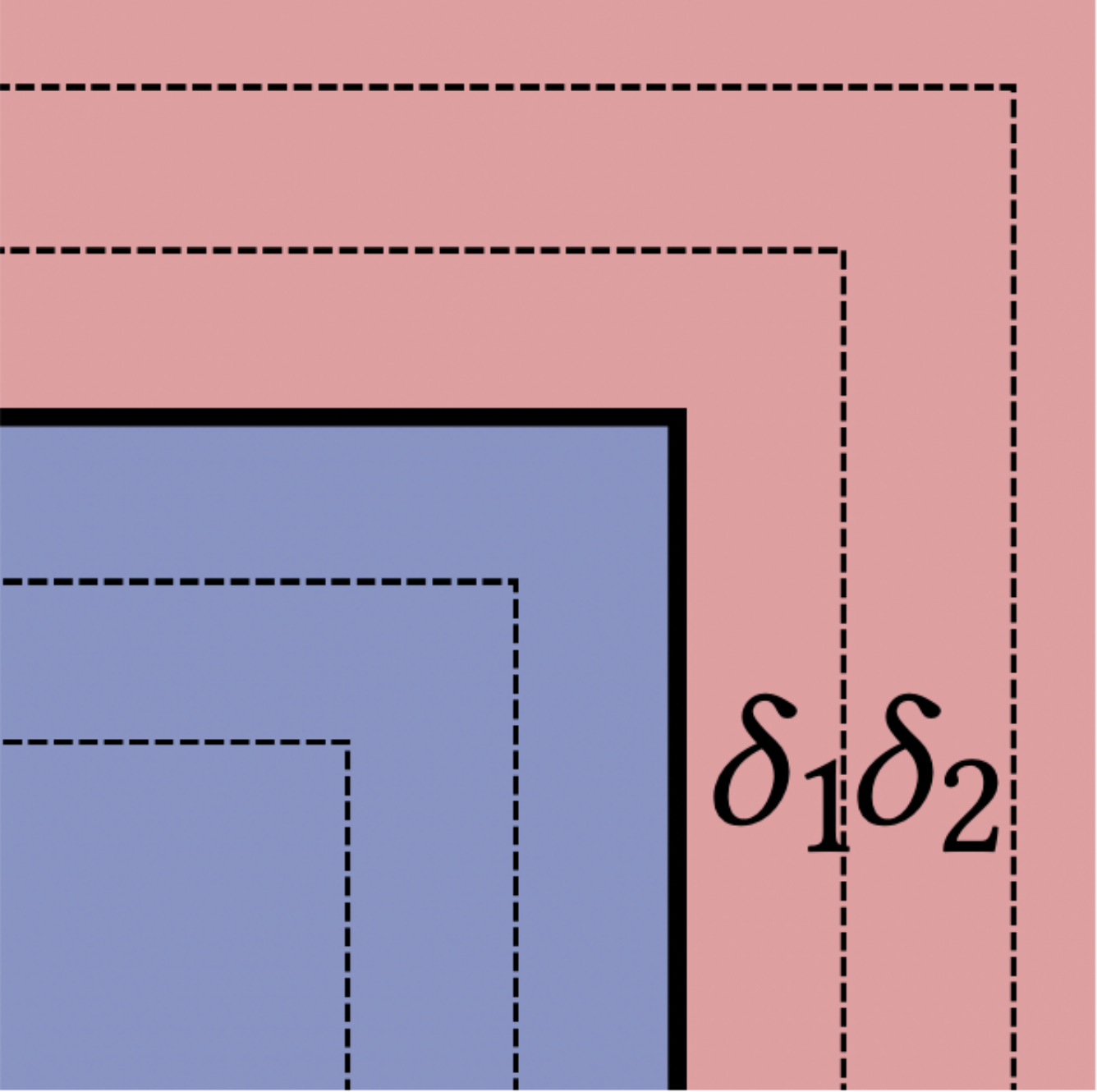
(a) GT shape

(b) Local SDF

(c) Global SDF

(d) Blended SDF

Figure 10. Given the blending region around the GT shape (a), the local SDF (b) and the global SDF (c) are blended to generate the blended SDF (d) that well preserves the sharp corner at its zero-level set and is globally defined in the whole domain.

Figure 11. We demonstrate the blending strategy in a 2D case.

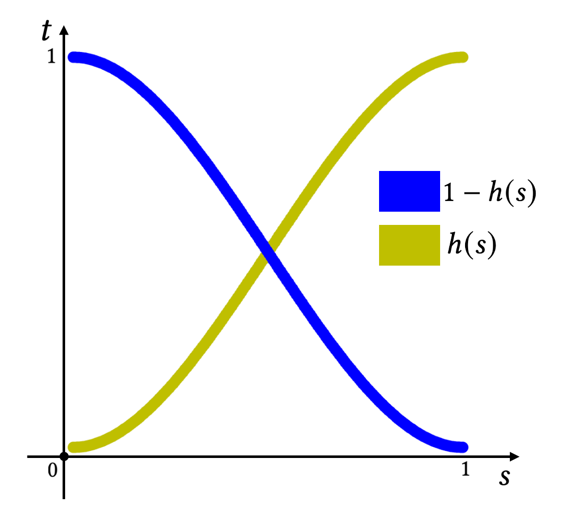
Figure 12. Weight functions for smooth interpolation.

With $F_{L}$ being a sufficiently accurate distance value for points near the surface $S$, we define three regions as follows: the region $R_{1}=\{\mathbf{x}|~{}|F_{L}(\mathbf{x})|<\delta_{1}\}$, $R_{2}=\{\mathbf{x}|\delta_{1}\leq|F_{L}(\mathbf{x})|\leq\delta_{2}\}$, and $R_{3}=D\setminus(R_{1}\cup R_{2})$, where $D$ is the entire bounding domain ($[-1,1]^{3}$) of a given shape. Then, we design the global feature-preserving distance function $F_{G}$. Inside the region $R_{1}$, we set $F_{P}=F_{L}$, because the local distance function $F_{L}$ is accurate and feature-preserving in $R_{1}$. In our implementation, with all shape bounding boxes as $[-1,1]^{3}$, we choose $\delta_{1}=0.001$ in the definition of $R_{1}$. In $R_{3}$, since $F_{L}$ becomes inaccurate and unstable because of the lack of supervision far from $S$, we set $F_{G}=F_{O}$. Similarly, we choose $\delta_{2}=0.03$ in the definition of $R_{3}$.

To make a smooth interpolation between $F_{L}$ and $F_{O}$ in $R_{2}$, we first define the weight functions $w_{0}(s)$ and $w_{1}(s)$ so that

(12) $$F_{G}(\mathbf{x})=w_{0}F_{L}(\mathbf{x})+w_{1}F_{O}(\mathbf{x}),~{}\mathbf{x}\in R_{2}.$$

Let us denote $d(\mathbf{x})=|F_{L}(\mathbf{x})|\in[\delta_{1},\delta_{2}],\mathbf{x}\in R_{2}$ and $s(\mathbf{x})=(d(\mathbf{x})-\delta_{1})/(\delta_{2}-\delta_{1})$ is a linear mapping maps $d(\mathbf{x})$ from $d(\mathbf{x})\in[\delta_{1},\delta_{2}]$ to $s(\mathbf{x})\in[0,1]$. We define the weight functions by

$$w_{0}(s)=(1-h(s(\mathbf{x})),w_{1}(s)=h(s(\mathbf{x}))$$

where $h(s)=3s^{2}-2s^{3}$, for $s\in[0,1]$; see Fig. 12.

Clearly, $h(0)=h^{\prime}(0)=h^{\prime}(1)=0$ and $h(1)=1$, from which one can verify that $F_{G}(\mathbf{x})=F_{L}(\mathbf{x})$ and $\nabla F_{G}(\mathbf{x})=\nabla F_{L}(\mathbf{x})$ along the inner boundaries of $R_{2}$ (i.e. where $|F_{L}(\mathbf{x})|=\delta_{1}$), and that $F_{G}(\mathbf{x})=F_{O}(\mathbf{x})$ and $\nabla F_{G}(\mathbf{x})=\nabla F_{O}(\mathbf{x})$ along the outer boundaries of $R_{2}$ (i.e. where $|F_{L}(\mathbf{x})|=\delta_{2}$). That is, $F_{G}$ thus defined is an $C^{1}$-continuous extension of $F_{L}$ in $R_{2}\cup R_{3}$. To summarize, the distance function $F_{G}(\mathbf{x})$ is a smooth blending of $F_{L}(\mathbf{x})$ and $F_{O}(\mathbf{x})$ and is globally defined on $D$. In particular, the zero-level set of $F_{G}$ agrees with that of $F_{L}(\mathbf{x})$, so it preserves the sharp features of the original target surface.

Finally, we show a 3D result of our blending strategy in Fig. 13 and demonstrate an offset application of our global distance function $F_{G}$ in Fig. 14.

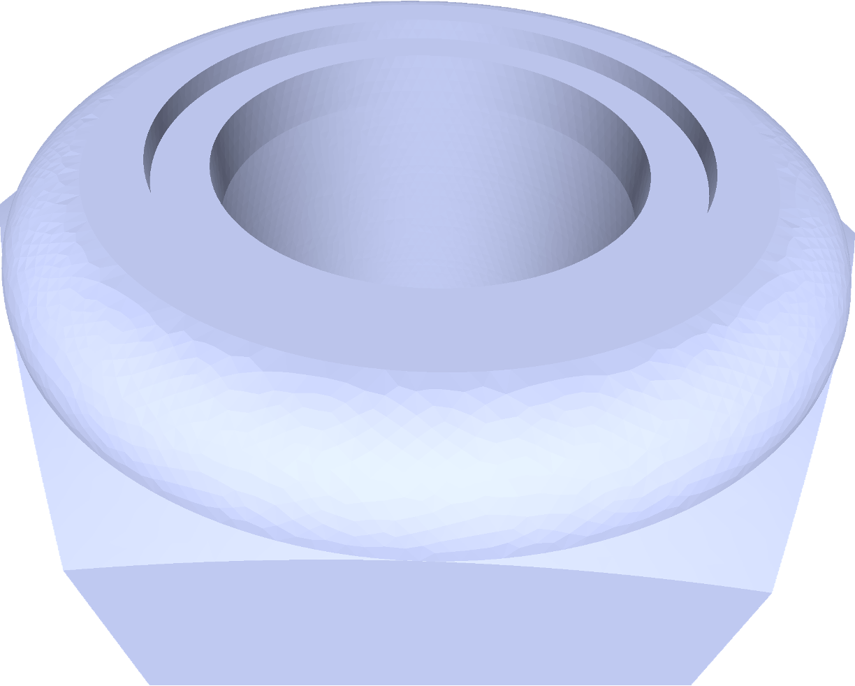
(a) GT shape

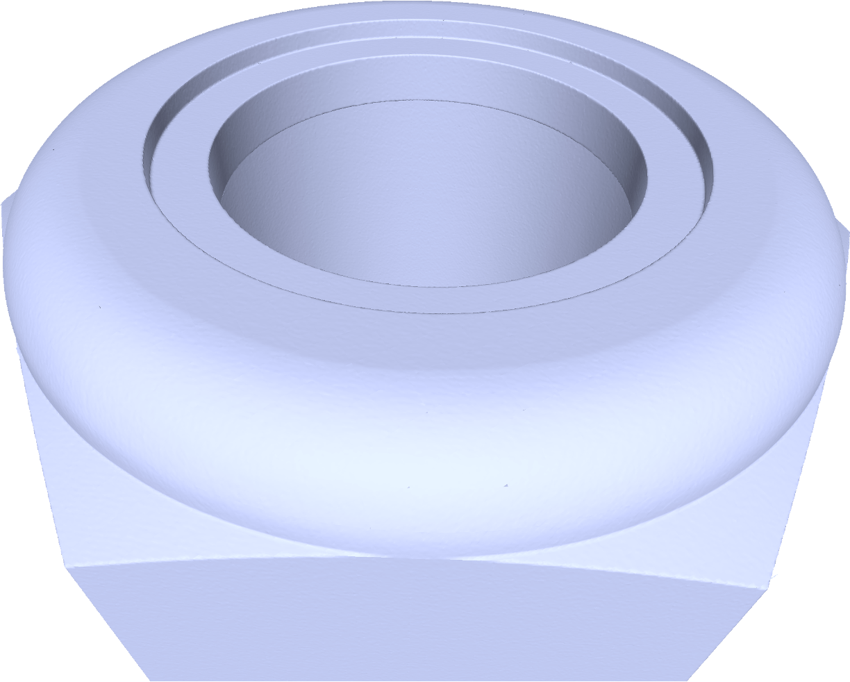
(b) Local SDF

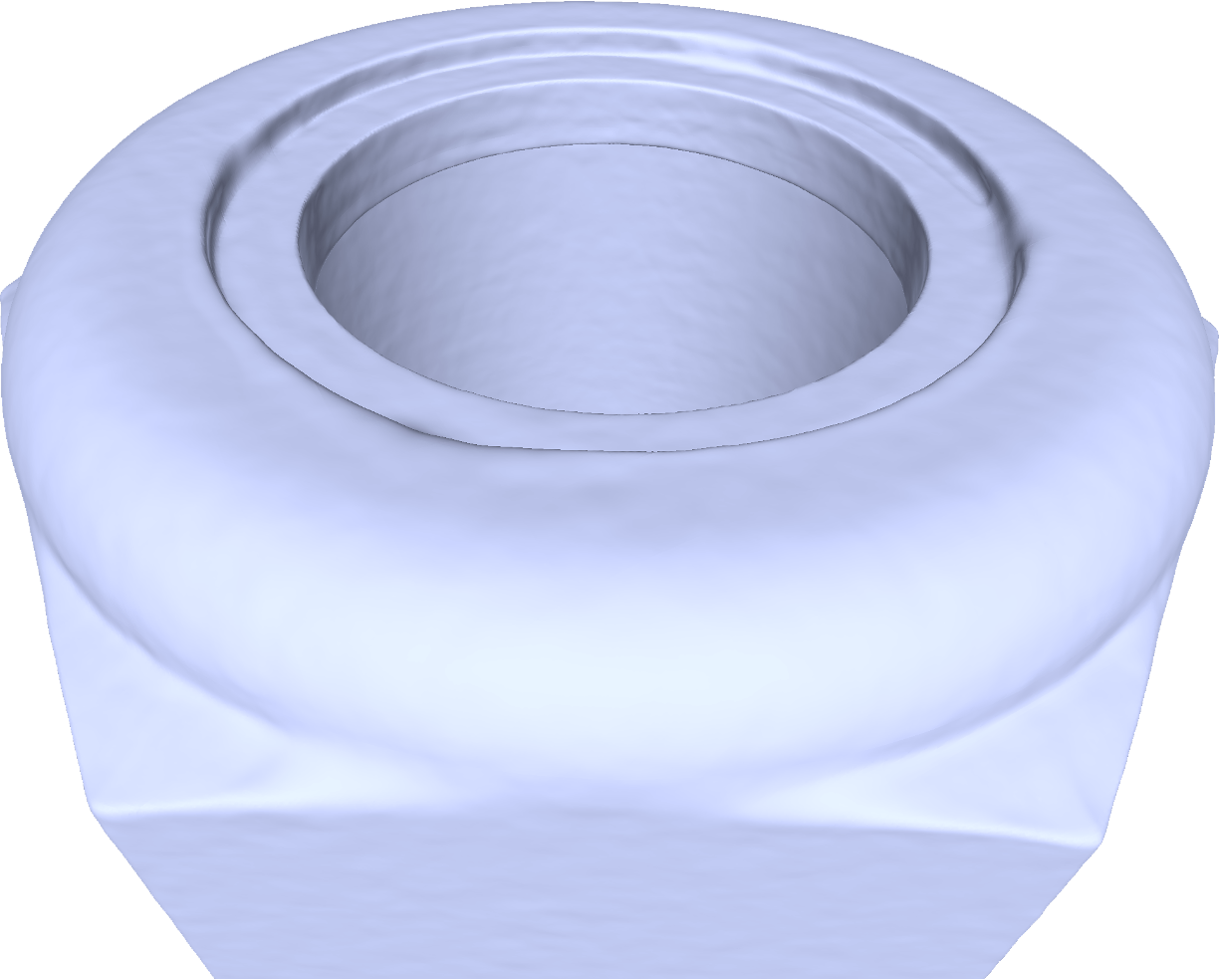
(c) Global SDF

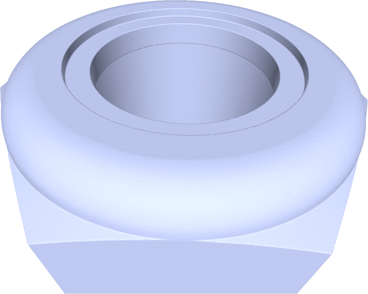
(d) Blended SDF

Figure 13. A 3D local case that merges the local and global SDF fields to form a blended SDF. We visualize the zero-level sets of the local, global, and blended SDFs in (b), (c), and (d), respectively. The zero-level set of the blended SDF (d) is faithful to the GT shape (a).

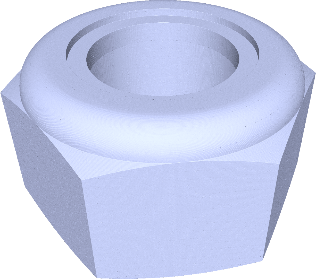
(a) Original zero-level surface

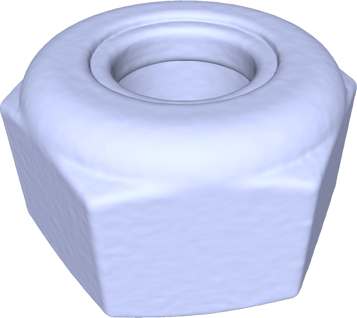
(b) Outer offset result

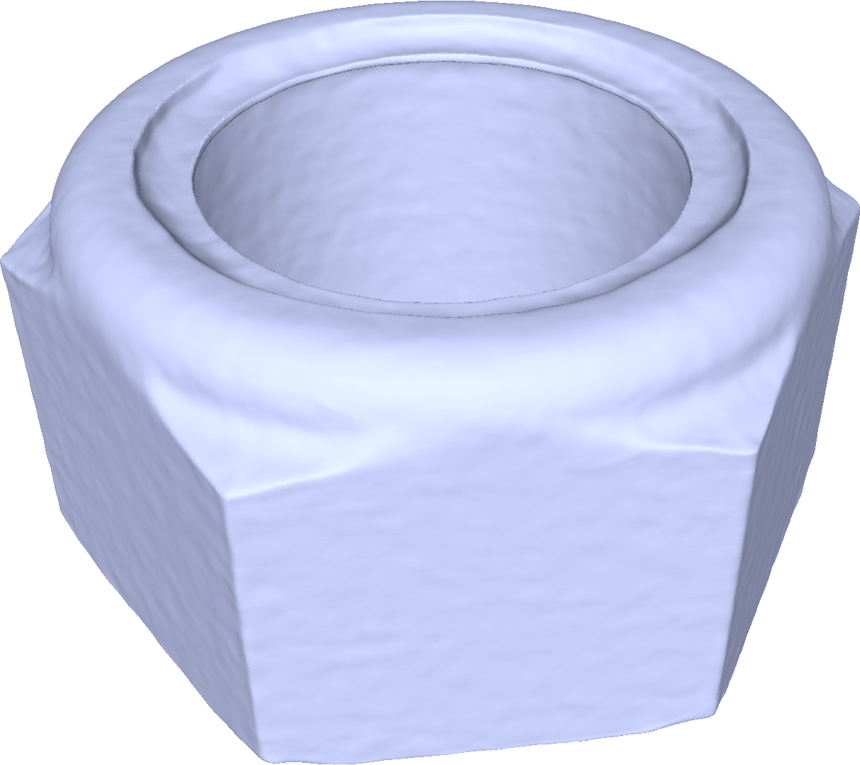
(c) Inner offset result

Figure 14. Offset application (b and c) with the blended SDF whose zero-level set is shown in (a).

5. Experimental results

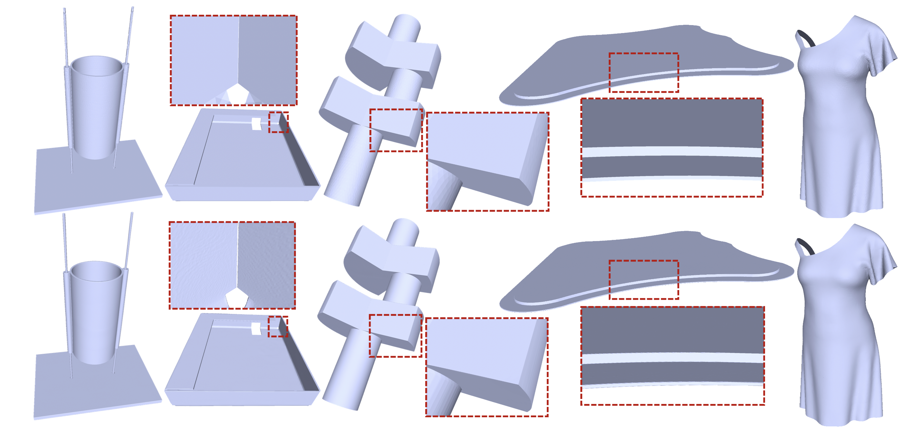
Figure 15. Our proposed approach, Patch-Grid, is capable of representing shapes that possess various types of features and demonstrates exceptional accuracy and robustness. (a, b): thin structures; (c, d): sharp boundary edges and corners; (e): clean boundary curves in the open surfaces.

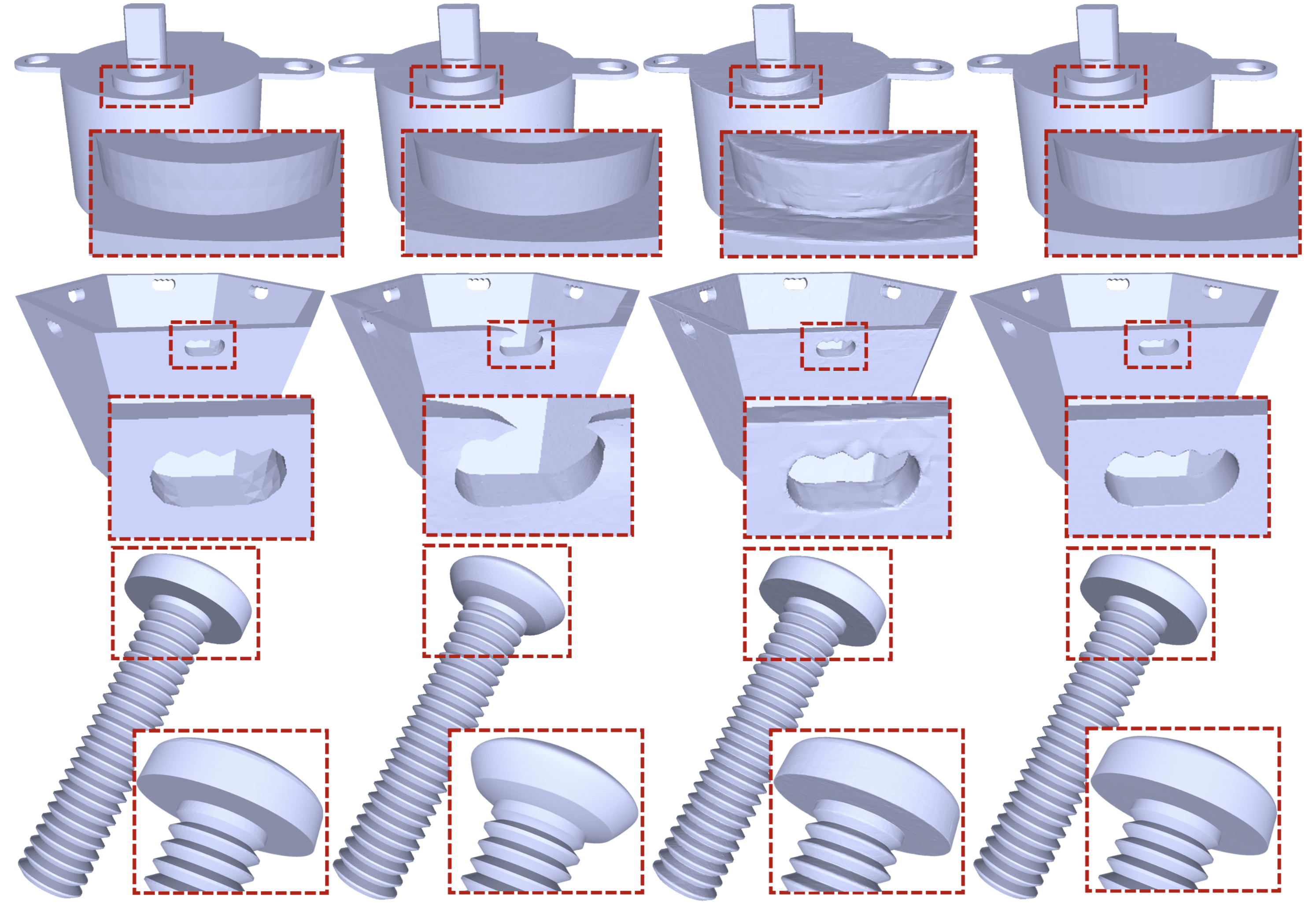
Figure 16. Comparison with NH-Rep (Guo et al., 2022) and NGLOD (Takikawa et al., 2021). Patch-Grid and NH-Rep, which adopt a patch-based representation, can faithfully capture sharp geometric features presented in the shapes, while NGLOD fails to do so, as shown in all the zoom-in views. Compared with NH-Rep, our local approach ensures robust performance in the presence of thin geometric features (in rows 2 and 3) that NH-Rep fails due to its global approach. The results produced by our method were obtained through an 8-second training phase, which demonstrates the efficiency of our method.

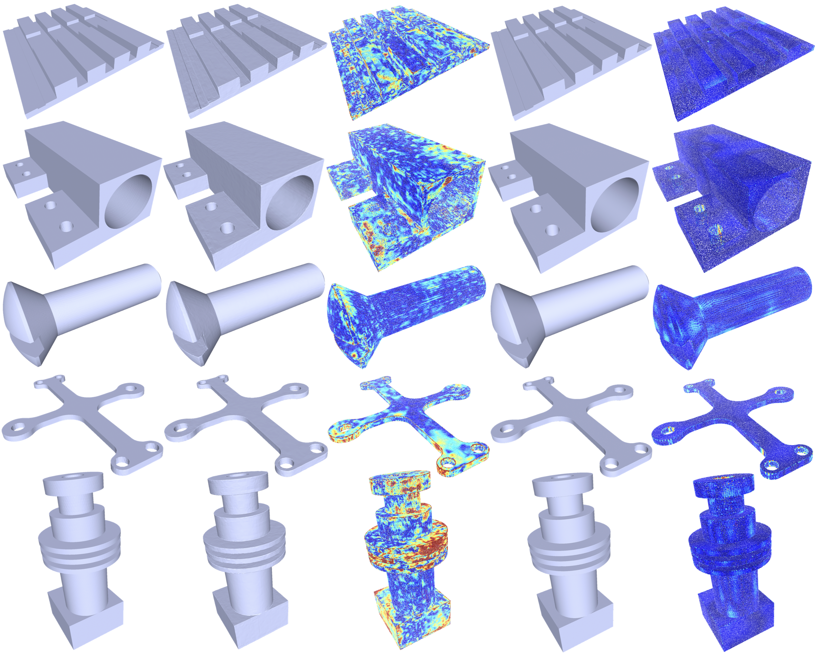
Figure 17. Detailed comparison with NGLOD (Takikawa et al., 2021). Columns (c) and (e) show the error distributions in terms of the Chamfer Distance between the reconstructed and GT meshes by NGLOD and Patch-Grid, respectively. The warmer color indicates a higher error, with the error being clipped by 0.001. Patch-Grid outperforms NGLOD significantly in terms of fitting accuracy, especially around the sharp features of the presented shapes.

5.1. Implementation details

Dataset and preprocessing

We test our method primarily on a data collection consisting of 100 CAD models sampled from the ABC dataset (Koch et al., 2019). All the shapes are segmented in advance and normalized to $[-1,1]^{3}$. For each segment of a given shape, we first construct a patch volume $V_{p}$. The resolution of the patch volume is determined by the average shape diameter (Shapira et al., 2008) of this segment computed with LIBIGL (Jacobson et al., 2018). Specifically, we stipulate that the size of the patch grid allocated to each patch should not exceed 2.5 times the average shape diameter of the patch. We observe that the resolution of a patch feature volume ranges from $2^{3}$ to $2^{6}$ depending on the local feature size. We construct the merge grid $\mathcal{G}$ as described in Sec. 3 and derive the merge constraints from the merge grid cells accordingly. We empirically set the maximal depth of the merge grid octree to 7.

Pretraining for shape update

In practice, it is often necessary to edit a 3D shape and update its corresponding implicit representation as well. Typically, the editing involves only a few patches. Therefore, to reuse the previously learned feature volumes while updating only the changed ones, we adopt the test-time optimization scheme, similar to (Park et al., 2019), to only update the patch feature volumes of the edited patches with the pretrained decoder fixed. We also allow using the fixed pretrained decoder to fit a completely new shape, which is denoted as Patch-Grid-PT. In this case, feature volumes of all patches are learnable.

Training details

We set the balance weights for the training loss terms as follows: $\lambda_{\mathrm{surface}}=150$, $\lambda_{\mathrm{normal}}=50$, $\lambda_{\mathrm{SDF}}=50$, $\lambda_{\mathrm{gradient}}=12$, $\lambda_{\mathrm{off}}=9$, $\lambda_{\mathrm{eikonal}}=12$, $\lambda_{\mathrm{code}}=1$, $\lambda_{\mathrm{merge}}=8$. We implemented the proposed method with PyTorch. ADAM (Kingma and Ba, 2015) with default hyperparameters is used as the optimizer for both pretraining and the fitting stages. Our fitting results were trained using 300 iterations. With an initial learning rate of 0.001, the learning rate is decayed by a factor of 0.3 at the 270th and 285th iterations. This training process takes about 8 seconds to fit a shape from scratch. For shape updating, our results were trained using 80 iterations with the same learning rate decay scheme at the 65-th and 72-th iterations. In each iteration, we globally sample 10,000 surface points and 10,000 spatial points off the surface and assign the sampled points to their corresponding cells. All results produced by our Patch-Grid and by the comparing methods were obtained on a desktop with a GPU card of NVIDIA RTX4090 and Intel i9 13900kf CPU. More implementation details can be found in our codes.

5.2. Evaluation metrics

To evaluate fitting accuracy, we use the following metrics: 1) the symmetric Chamfer distance (CD); 2) the F-score based on CD; 3) the Hausdorff distance (HD); and 4) the normal consistency (NC). The symmetric Chamfer distance measures the averaged reconstruction quality of a given shape. The Hausdorff distance is the maximum reconstruction error either from the reconstruction to the ground-truth (GT) mesh or from the GT mesh to the reconstruction. The normal consistency measures how similar the normal vectors at the reconstructed surface are to those at the GT mesh surface. We also report F-score, a statistical measure, to show the overall quality of the reconstruction quality. Specifically, the F-score is computed as the percentage of points with a reconstruction error smaller than $0.001$ throughout the paper. In all experiments, we sample 300k points from the extracted surface and another 300k from the ground-truth mesh. Then we compute the two-sided closest point-to-surface distances to evaluate all metrics.

5.3. Results and discussions

Shape fitting

Our method can model 3D surface shapes with various geometry features, e.g., narrow gaps, sharp features, or open boundaries, at high fidelity as is shown in Fig 1(a) and Fig. 15.

We report the quantitative results in Tab. 1 produced by two variants of our approach (Patch-Grid and Patch-Grid-PT) and the state-of-the-art (SOTA) methods and compare them to the results produced by NH-Rep (Guo et al., 2022) and NGLOD (Takikawa et al., 2021) on two subsets of shapes randomly drawn from the ABC dataset, respectively. A subset of 100 shapes is used in the comparison with NH-Rep, whereas 10 shapes are randomly sampled for the comparison with NGLOD due to its prolonged training time. Patch-Grid denotes training our approach trained from scratch, while Patch-Grid-PT denotes training our approach with a fixed, pretrained decoder as described in the previous subsection. For the methods tested on the pool of 10 shapes, we added a suffix of $*$ to denote them as NGLOD*, Patch-Grid*, and Patch-Grid-PT*.

Our approach, in both its variants (Patch-Grid and Patch-Grid-PT), can achieve significantly better reconstruction performance than NH-Rep and NGLOD as indicated by the metrics. As we noted that there are some severe failure cases in NH-Rep due to its robustness issue as discussed earlier, we do not include these shapes in the quantitative comparison, and our approach still performs favorably as compared to NH-Rep. We attribute this performance gain to the use of the adaptive merge grid, which circumvents the difficulty in managing the extended zero-level sets of the learned patches to satisfy the global CSG constraints.

The training time for an object is typically around 8 seconds, taking 300 iterations, which is $23\times$ and $287\times$ speed-up as compared with NH-Rep (3 minutes) and NGLOD (38 minutes), respectively. Hence, our method brings about a significant improvement over the other comparing methods in both computational efficiency and fitting accuracy.

Table 1. Quantitative evaluation of different neural implicit representations in terms of the symmetric Chamfer distance (CD), F-score (CD ¡ 0.001), Hausdorff distance (HD), and normal consistency (NC). $\uparrow$ indicates the higher the better, while $\downarrow$ indicates the lower the better. CD, HD and NC are presented in units of $\times 10^{-4}$, $\times 10^{-3}$ and $\times 10^{-2}$, respectively. We also report the training time in the unit of seconds.

Metrics	CD $\downarrow$	F-score $\uparrow$	HD $\downarrow$	NC $\downarrow$	Time $\downarrow$
NH-Rep	6.7	92.44	6.9	6.791	185
Patch-Grid	1.0	99.19	3.0	6.464	8
Patch-Grid-PT	1.5	99.39	2.7	6.430	8
NGLOD*	2.7	97.99	3.8	10.15	2296
Patch-Grid*	0.7	99.75	1.4	4.841	8
Patch-Grid-PT*	1.6	99.85	1.5	5.412	8

For qualitative comparison, we show several results produced by Patch-Grid and the other methods in Fig. 16. Compared with NH-Rep which also uses a patch-wise representation, Patch-Grid can robustly model geometric features presented in shapes as shown in the bottom two rows of Fig. 16. NH-Rep adopts a global approach to assembling the learned implicit functions into the target shape, which is prone to fail due to the undesirable interference between the extraneous zero-level sets of the individual learned implicit patches. In contrast, Patch-Grid consistently produces robust, high-quality results even in these challenging cases, validating the superiority of the proposed local approach.

We also compare Patch-Grid to NGLOD, which models the entire shape without decomposition. Different from NGLOD, both NH-Rep and Patch-Grid are based on patch decomposition and therefore can faithfully model the sharp features presented in the 3D shapes as shown in the zoom-in views in Fig. 17. Here, we visualize the reconstruction error maps of our results and those of NGLOD regarding five additional shapes, which show that Patch-Grid consistently obtains smaller fitting errors for the five shapes than NGLOD. This superior accuracy is attributed to the use of patch-based representation, partly because it reduces our learning task to fit a small number of patches in each merge grid cell locally instead of modeling a complex shape as is done for NGLOD and partly because Patch-Grid is capable of sharp features by composing several learned patches.

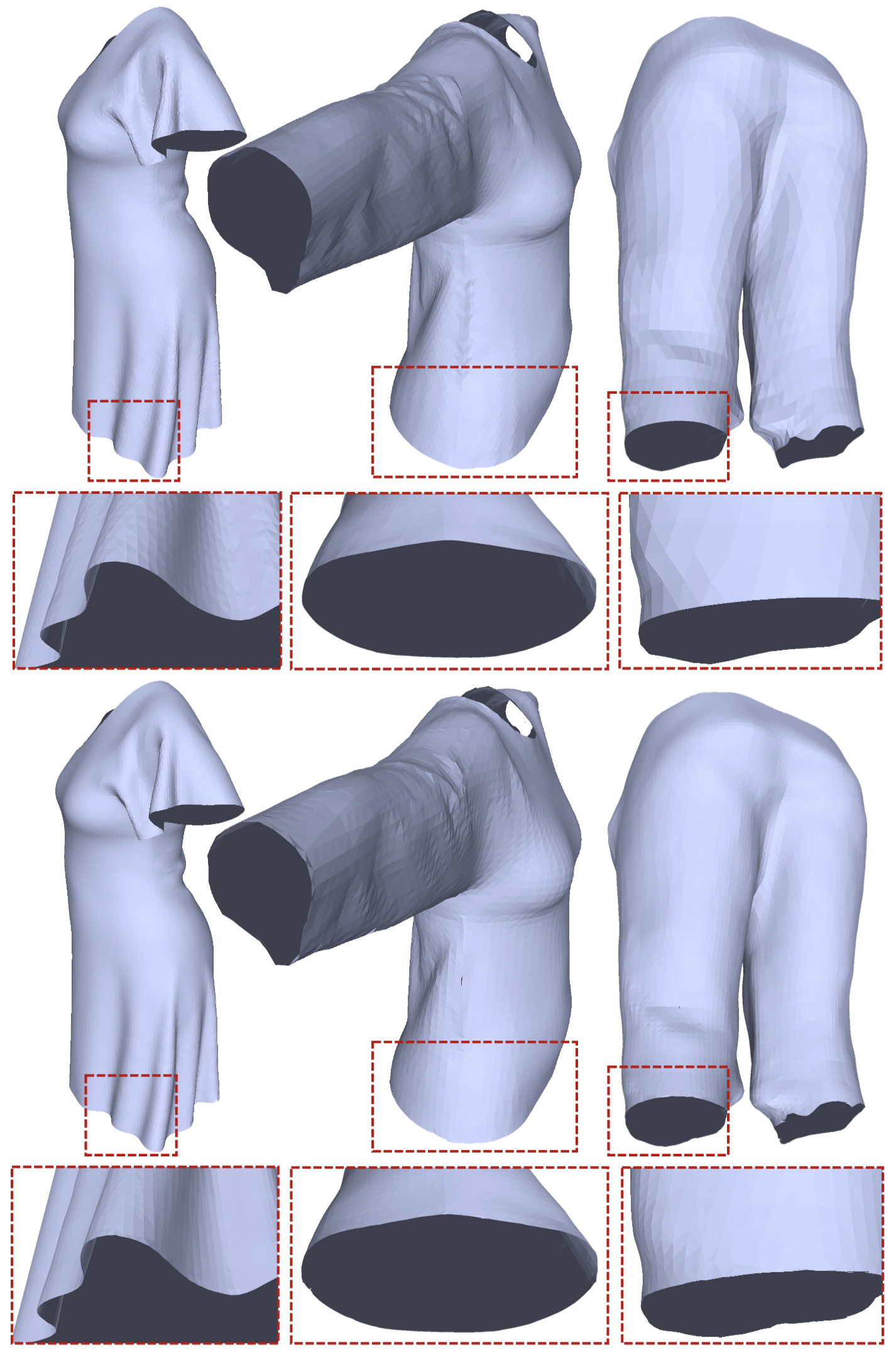
Figure 18. Examples of open surfaces with the zoom-in views at the open surface boundaries. Patch-Grid, modeling the open surface boundaries via a trimming process, cuts the boundaries in a precise and clean manner.

In addition to the CAD models and those models with thin geometric features in Figs. 7, we also show in Fig. 18 the reconstruction results of three garment models (i.e., a dress from VTO (Santesteban et al., 2019) and a shirt and a pair of pants from MGN  (Bhatnagar et al., 2019)) with open surface boundaries to demonstrate the representational capability of the proposed method for modeling open surface boundaries. As shown, Patch-Grid produces accurately reproduces the open surface boundaries.

Shape editing

We have demonstrated a few updated shapes in Fig. 1(b) earlier. Now we show more shape updating results in Fig. 19. All the results are shown in Fig. 1(b) and Fig. 19 take only 1 second of training to complete with the Patch-Grid-PT setting where only the feature volumes of the edited patches were updated.

We applied a variety of editing operations to the shape shown in Fig. 19, such as adding a trimming surface to form a chamfer to the central hole as in Fig. 19(e). In each edited shape, we highlight the modified patches in orange. Additionally, the connected patches that are not directly edited but are affected by the update of the merge constraints are highlighted in green. Both the edited and involved patches are updated while the rest of the patches are kept fixed.

The fitting accuracy regarding these edited shapes is reported in Tab. 2, which is similar to the performance obtained in the shape fitting task, demonstrating the consistently superior performance of our method in both shape fitting and updating tasks.

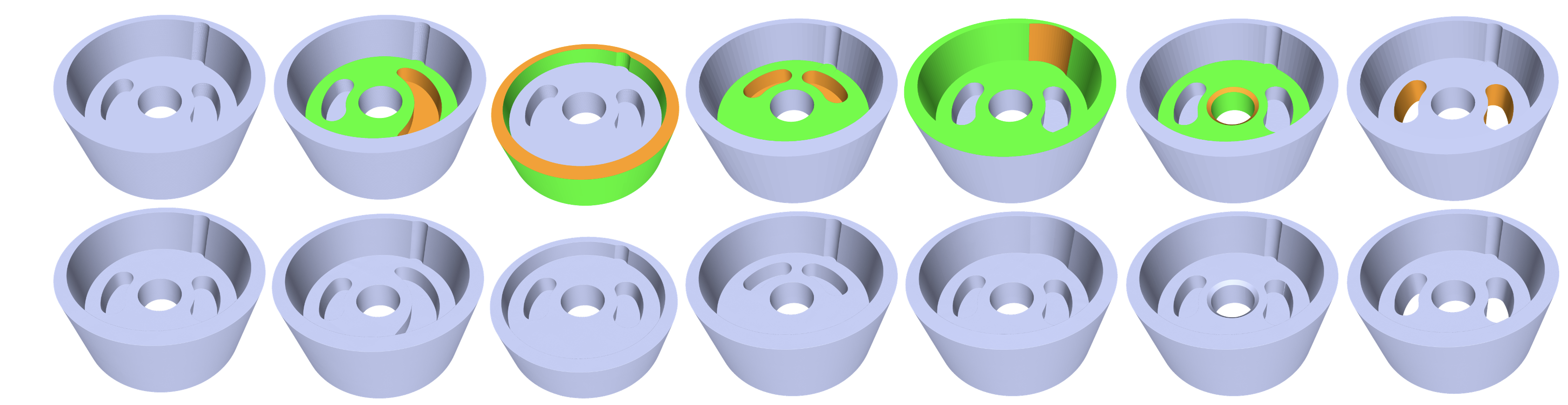
Figure 19. A collection of edited shapes (top) and the results (bottom) fitted by our shape updating strategy is presented. A variety of editing operations are applied to the original shape in (a). (b): free-form deformation of the circular slot; (c): parametric editing of the height of the top; (d) rigid transformation of the pair of circular slots; (e): parametric editing of the radius of the cylindrical patch; (f): adding a new patch to create a chamfer to the central through-hole; (g): Extending several patches and removing two patches to obtain a pair of penetrated slots. In each edited shape, the modified patches are highlighted in orange. Additionally, the connected patches that are not directly edited but are affected by the changes due to merge constraints are also highlighted in green. Patch feature volumes of both the directly edited and affected patches are updated while the rest of the patch feature volumes remain fixed.

Table 2. Quantitative evaluation of the edited shapes. The accuracy of the edited shape is consistent with the accuracy of shape fitting. CD, HD and NC are presented in units of $\times 10^{-4}$, $\times 10^{-3}$ and $\times 10^{-2}$, respectively. The training time is in the unit of seconds.

CD $\downarrow$	F-score $\uparrow$	HD $\downarrow$	NC $\downarrow$	Time $\downarrow$
1.8	98.84	3.1	3.504	1

5.4. Ablation study

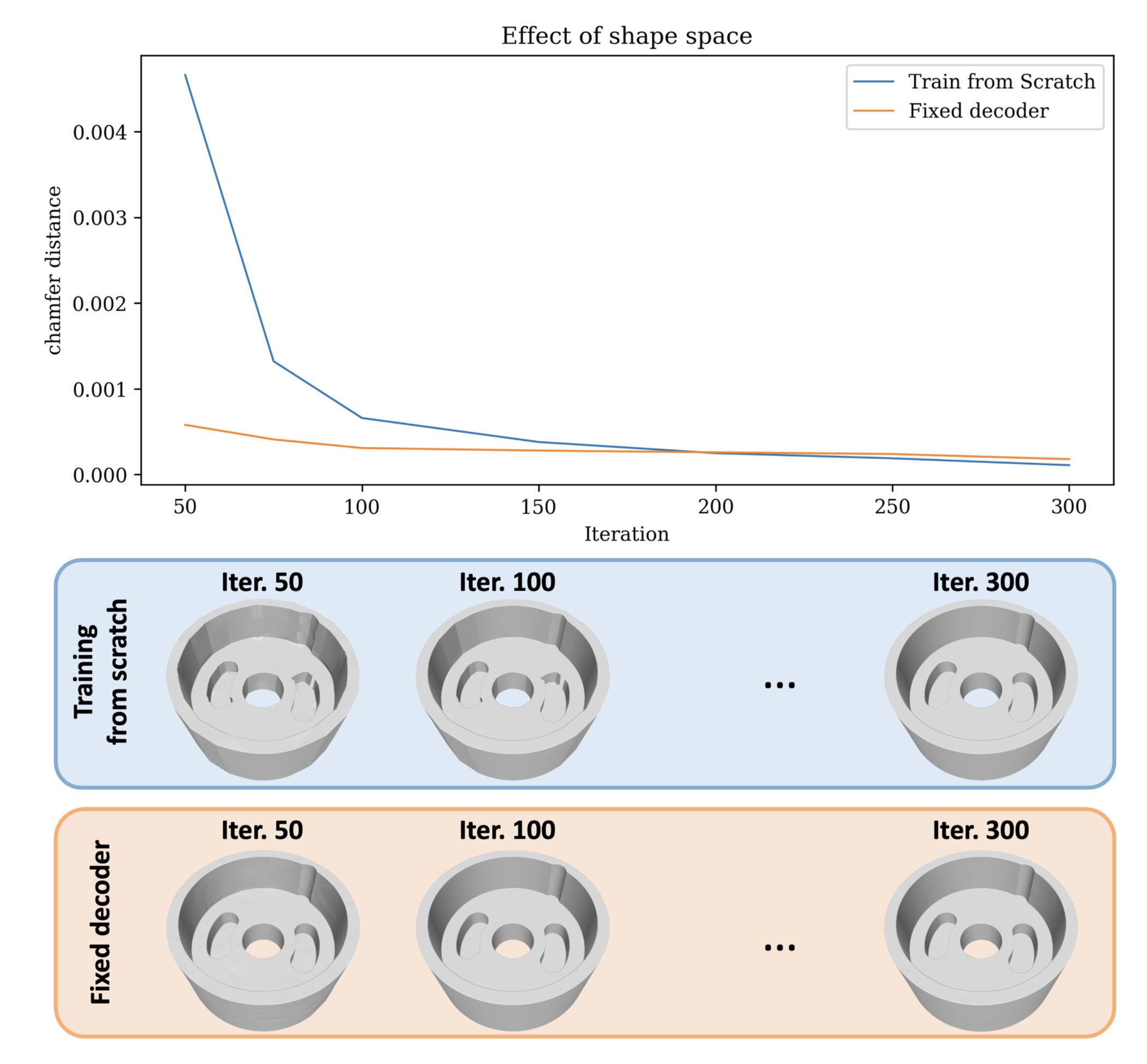
Figure 20. Pretrained fixed shape space matters. The ablation reveals that the use of a fixed, pretrained decoder significantly accelerates training as shown by the curves of CD value against the number of iterations (around 100 iterations). In contrast, without pretraining, our method takes 200 iterations to converge. The impact of the pretrained shape space is also evident in the visualization of the shapes, as demonstrated in the following figures.

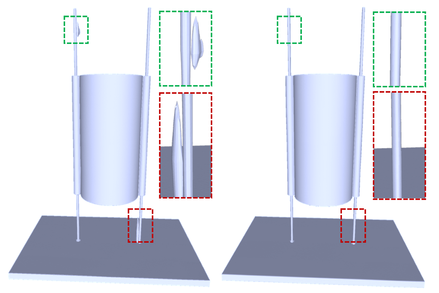
Figure 21. Adaptive patch volumes matter. (a) Without the use of adaptive patch volumes, the resulting shape extracted from the compositional neural signed distance field may have artifacts observed around the thin components due to the uniform resolution used across different patches; (b) Using adaptive patch volumes can effectively resolve the issue, showing the necessity for the proposed method.

We conducted ablation studies to validate the use of the adaptive patch volumes by ablating this design choice, denoted w/o Ada-PV. Tab. 3 shows that w/o Ada-PV yields less satisfactory results. A qualitative example is provided in Fig. 21 to show the necessity of adaptive patch volumes for modeling slender geometry; otherwise, using patch volumes of uniform size fails to accurately fit thin tubes.

Regarding the two previously introduced training schemes: 1) with a trainable decoder from scratch; and 2) with a fixed pretrained decoder, we conducted an experiment to show their respective advantages. Both schemes were used to fit the data collection of 100 shapes and the results are reported Tab. 3. We see that training the decoder from scratch (i.e., scheme 1) can achieve slightly favorable results in terms of the Chamfer distance and F-score. Yet, Scheme 1 (Train from Scratch) converges slower (around 300 iterations, or 8 seconds) than Scheme 2 (Fixed decoder) which requires around 100 iterations, or 3 seconds as shown in Fig. 20.

Table 3. Quantitative results of the ablation. It shows using adaptive resolutions for different patch volumes leads to better performance. Similar performance gain can be achieved by the two variants of our method. CD, HD and NC are presented in units of $\times 10^{-4}$, $\times 10^{-3}$ and $\times 10^{-2}$, respectively.

	CD $\downarrow$	F-score $\uparrow$	HD $\downarrow$	NC $\downarrow$
Train from Scratch	1.0	99.19	3.0	6.464
Fixed decoder	1.5	99.39	2.7	6.430
w/o Ada-PV	7.7	98.56	12	6.608

6. Conclusion

We have presented a novel implicit neural surface using a patch-based representation with a grid-based local training and merging strategy. Patch-Grid performs CSG operations locally in grid-based cells to significantly improve the robustness of the patch-based representation, compared with the prior work (Guo et al., 2022) using a global approach. Moreover, Patch-Grid is capable of dealing with a wide variety of shapes including thin geometries, open surfaces. We evaluate Patch-Grid on various 3D shapes to validate its superiority to existing works in terms of robustness, efficiency, accuracy, and versatility.

There are several limitations to our method. (1) Patch-Grid assumes a preprocessing stage that provides us with meaningful segmentation for models. A shape segmentation procedure is needed as a preprocessing step for our method. (2) Currently, Patch-Grid cannot represent non-manifold surfaces, which is a task that would need further research. Furthermore, it is an interesting topic for future research to explore the potential of Patch-Grid to support structure-level or semantic-level shape editing and shape manipulation due to its flexible representation with patch-wise latent spaces.

References

- (1)
- Allen (2021) George Allen. 2021. nTopology’s Implicit Modeling Technology. https://ntopology.com/resources/whitepaper-implicit-modeling-technology/. Last accessed 2021-12-1.
- Amenta and Bern (1998) Nina Amenta and Marshall Bern. 1998. Surface reconstruction by Voronoi filtering. In Proceedings of the fourteenth annual symposium on Computational geometry. 39–48.
- Bhatnagar et al. (2019) Bharat Lal Bhatnagar, Garvita Tiwari, Christian Theobalt, and Gerard Pons-Moll. 2019. Multi-Garment Net: Learning to Dress 3D People from Images. In IEEE International Conference on Computer Vision (ICCV). IEEE.
- Chen et al. (2022) Weikai Chen, Cheng Lin, Weiyang Li, and Bo Yang. 2022. 3PSDF: Three-Pole Signed Distance Function for Learning Surfaces With Arbitrary Topologies. In Proceedings of the IEEE/CVF Conference on Computer Vision and Pattern Recognition (CVPR). 18522–18531.
- Chen and Zhang (2019) Zhiqin Chen and Hao Zhang. 2019. Learning Implicit Fields for Generative Shape Modeling. In Proceedings of the IEEE/CVF Conference on Computer Vision and Pattern Recognition (CVPR).
- Chibane et al. (2020) Julian Chibane, Mohamad Aymen mir, and Gerard Pons-Moll. 2020. Neural Unsigned Distance Fields for Implicit Function Learning. In Advances in Neural Information Processing Systems, H. Larochelle, M. Ranzato, R. Hadsell, M.F. Balcan, and H. Lin (Eds.), Vol. 33. Curran Associates, Inc., 21638–21652. https://proceedings.neurips.cc/paper/2020/file/f69e505b08403ad2298b9f262659929a-Paper.pdf
- Davies et al. (2020) Thomas Davies, Derek Nowrouzezahrai, and Alec Jacobson. 2020. On the Effectiveness of Weight-Encoded Neural Implicit 3D Shapes. https://doi.org/10.48550/ARXIV.2009.09808
- Duan et al. (2020) Yueqi Duan, Haidong Zhu, He Wang, Li Yi, Ram Nevatia, and Leonidas J. Guibas. 2020. Curriculum DeepSDF. In Computer Vision – ECCV 2020, Andrea Vedaldi, Horst Bischof, Thomas Brox, and Jan-Michael Frahm (Eds.). Springer International Publishing, Cham, 51–67.
- Genova et al. (2020) Kyle Genova, Forrester Cole, Avneesh Sud, Aaron Sarna, and Thomas Funkhouser. 2020. Local Deep Implicit Functions for 3D Shape. In Proceedings of the IEEE/CVF Conference on Computer Vision and Pattern Recognition (CVPR).
- Gropp et al. (2020) Amos Gropp, Lior Yariv, Niv Haim, Matan Atzmon, and Yaron Lipman. 2020. Implicit Geometric Regularization for Learning Shapes. In Proceedings of the 37th International Conference on Machine Learning (Proceedings of Machine Learning Research, Vol. 119), Hal Daumé III and Aarti Singh (Eds.). PMLR, 3789–3799. https://proceedings.mlr.press/v119/gropp20a.html
- Guo et al. (2022) Hao-Xiang Guo, Yang Liu, Hao Pan, and Baining Guo. 2022. Implicit Conversion of Manifold B-Rep Solids by Neural Halfspace Representation. ACM Trans. Graph. 41, 6, Article 276 (nov 2022), 15 pages. https://doi.org/10.1145/3550454.3555502
- Jacobson et al. (2018) Alec Jacobson, Daniele Panozzo, et al. 2018. libigl: A simple C++ geometry processing library. https://libigl.github.io/.
- Jiang et al. (2020) Chiyu ”Max” Jiang, Avneesh Sud, Ameesh Makadia, Jingwei Huang, Matthias Niessner, and Thomas Funkhouser. 2020. Local Implicit Grid Representations for 3D Scenes. In Proceedings of the IEEE/CVF Conference on Computer Vision and Pattern Recognition (CVPR).
- Kingma and Ba (2015) Diederik P. Kingma and Jimmy Ba. 2015. Adam: A Method for Stochastic Optimization. In 3rd International Conference on Learning Representations, ICLR 2015, San Diego, CA, USA, May 7-9, 2015, Conference Track Proceedings, Yoshua Bengio and Yann LeCun (Eds.). http://arxiv.org/abs/1412.6980
- Koch et al. (2019) Sebastian Koch, Albert Matveev, Zhongshi Jiang, Francis Williams, Alexey Artemov, Evgeny Burnaev, Marc Alexa, Denis Zorin, and Daniele Panozzo. 2019. ABC: A Big CAD Model Dataset for Geometric Deep Learning. In Proceedings of the IEEE/CVF Conference on Computer Vision and Pattern Recognition (CVPR).
- Li et al. (2011) Yangyan Li, Xiaokun Wu, Yiorgos Chrysathou, Andrei Sharf, Daniel Cohen-Or, and Niloy J. Mitra. 2011. GlobFit: Consistently Fitting Primitives by Discovering Global Relations. In ACM SIGGRAPH 2011 Papers (Vancouver, British Columbia, Canada) (SIGGRAPH ’11). Association for Computing Machinery, New York, NY, USA, Article 52, 12 pages. https://doi.org/10.1145/1964921.1964947
- Martel et al. (2021) Julien NP Martel, David B Lindell, Connor Z Lin, Eric R Chan, Marco Monteiro, and Gordon Wetzstein. 2021. ACORN: Adaptive Coordinate Networks for Neural Scene Representation. arXiv preprint arXiv:2105.02788 (2021).
- Mescheder et al. (2019) Lars Mescheder, Michael Oechsle, Michael Niemeyer, Sebastian Nowozin, and Andreas Geiger. 2019. Occupancy Networks: Learning 3D Reconstruction in Function Space. In Proceedings of the IEEE/CVF Conference on Computer Vision and Pattern Recognition (CVPR).
- Mitchell et al. (2015) Nathan Mitchell, Mridul Aanjaneya, Rajsekhar Setaluri, and Eftychios Sifakis. 2015. Non-manifold level sets: A multivalued implicit surface representation with applications to self-collision processing. ACM Transactions on Graphics (TOG) 34, 6 (2015), 1–9.
- Müller et al. (2022) Thomas Müller, Alex Evans, Christoph Schied, and Alexander Keller. 2022. Instant neural graphics primitives with a multiresolution hash encoding. ACM Transactions on Graphics (ToG) 41, 4 (2022), 1–15.
- Nan and Wonka (2017) Liangliang Nan and Peter Wonka. 2017. PolyFit: Polygonal Surface Reconstruction From Point Clouds. In Proceedings of the IEEE International Conference on Computer Vision (ICCV).
- Ohtake et al. (2005) Yutaka Ohtake, Alexander Belyaev, Marc Alexa, Greg Turk, and Hans-Peter Seidel. 2005. Multi-level partition of unity implicits. In Acm Siggraph 2005 Courses. 173–es.
- Park et al. (2019) Jeong Joon Park, Peter Florence, Julian Straub, Richard Newcombe, and Steven Lovegrove. 2019. DeepSDF: Learning Continuous Signed Distance Functions for Shape Representation. In Proceedings of the IEEE/CVF Conference on Computer Vision and Pattern Recognition (CVPR).
- Santesteban et al. (2019) Igor Santesteban, Miguel A. Otaduy, and Dan Casas. 2019. Learning-Based Animation of Clothing for Virtual Try-On. Computer Graphics Forum (Proc. Eurographics) (2019). https://doi.org/10.1111/cgf.13643
- Schnabel et al. (2007) R. Schnabel, R. Wahl, and R. Klein. 2007. Efficient RANSAC for Point-Cloud Shape Detection. Computer Graphics Forum 26, 2 (2007), 214–226. https://doi.org/10.1111/j.1467-8659.2007.01016.x arXiv:https://onlinelibrary.wiley.com/doi/pdf/10.1111/j.1467-8659.2007.01016.x
- Shapira et al. (2008) Lior Shapira, Ariel Shamir, and Daniel Cohen-Or. 2008. Consistent mesh partitioning and skeletonisation using the shape diameter function. The Visual Computer 24 (2008), 249–259.
- Sitzmann et al. (2020a) Vincent Sitzmann, Eric R Chan, Richard Tucker, Noah Snavely, and Gordon Wetzstein. 2020a. Metasdf: Meta-learning signed distance functions. arXiv preprint arXiv:2006.09662 (2020).
- Sitzmann et al. (2020b) Vincent Sitzmann, Julien Martel, Alexander Bergman, David Lindell, and Gordon Wetzstein. 2020b. Implicit Neural Representations with Periodic Activation Functions. In Advances in Neural Information Processing Systems, H. Larochelle, M. Ranzato, R. Hadsell, M.F. Balcan, and H. Lin (Eds.), Vol. 33. Curran Associates, Inc., 7462–7473. https://proceedings.neurips.cc/paper/2020/file/53c04118df112c13a8c34b38343b9c10-Paper.pdf
- Takikawa et al. (2021) Towaki Takikawa, Joey Litalien, Kangxue Yin, Karsten Kreis, Charles Loop, Derek Nowrouzezahrai, Alec Jacobson, Morgan McGuire, and Sanja Fidler. 2021. Neural Geometric Level of Detail: Real-Time Rendering With Implicit 3D Shapes. In Proceedings of the IEEE/CVF Conference on Computer Vision and Pattern Recognition (CVPR). 11358–11367.
- Tancik et al. (2020a) Matthew Tancik, Pratul Srinivasan, Ben Mildenhall, Sara Fridovich-Keil, Nithin Raghavan, Utkarsh Singhal, Ravi Ramamoorthi, Jonathan Barron, and Ren Ng. 2020a. Fourier Features Let Networks Learn High Frequency Functions in Low Dimensional Domains. In Advances in Neural Information Processing Systems, H. Larochelle, M. Ranzato, R. Hadsell, M.F. Balcan, and H. Lin (Eds.), Vol. 33. Curran Associates, Inc., 7537–7547. https://proceedings.neurips.cc/paper/2020/file/55053683268957697aa39fba6f231c68-Paper.pdf
- Tancik et al. (2020b) Matthew Tancik, Pratul P Srinivasan, Ben Mildenhall, Sara Fridovich-Keil, Nithin Raghavan, Utkarsh Singhal, Ravi Ramamoorthi, Jonathan T Barron, and Ren Ng. 2020b. Fourier features let networks learn high frequency functions in low dimensional domains. arXiv preprint arXiv:2006.10739 (2020).
- Tretschk et al. (2020) Edgar Tretschk, Ayush Tewari, Vladislav Golyanik, Michael Zollhöfer, Carsten Stoll, and Christian Theobalt. 2020. PatchNets: Patch-Based Generalizable Deep Implicit 3D Shape Representations. In Computer Vision – ECCV 2020, Andrea Vedaldi, Horst Bischof, Thomas Brox, and Jan-Michael Frahm (Eds.). Springer International Publishing, Cham, 293–309.
- Turk and O’brien (2002) Greg Turk and James F O’brien. 2002. Modelling with implicit surfaces that interpolate. ACM Transactions on Graphics (TOG) 21, 4 (2002), 855–873.
- Zhang et al. (2022) Congyi Zhang, Mohamed Elgharib, Gereon Fox, Min Gu, Christian Theobalt, and Wenping Wang. 2022. An Implicit Parametric Morphable Dental Model. ACM Trans. Graph. 41, 6, Article 217 (nov 2022), 13 pages. https://doi.org/10.1145/3550454.3555469