Random projection using random quantum circuits
Abstract
The random sampling task performed by Google’s Sycamore processor gave us a glimpse of the ”Quantum Supremacy era”. This has definitely shed some spotlight on the power of random quantum circuits in this abstract task of sampling outputs from the (pseudo-) random circuits. In this manuscript, we explore a practical near-term use of local random quantum circuits in dimensional reduction of large low-rank data sets. We make use of the well-studied dimensionality reduction technique called the random projection method. This method has been extensively used in various applications such as image processing, logistic regression, entropy computation of low-rank matrices, etc. We prove that the matrix representations of local random quantum circuits with sufficiently shorter depths () serve as good candidates for random projection. We demonstrate numerically that their projection abilities are not far off from the computationally expensive classical principal components analysis on MNIST and CIFAR-100 image data sets. We also benchmark the performance of quantum random projection against the commonly used classical random projection in the tasks of dimensionality reduction of image datasets and computing Von Neumann entropies of large low-rank density matrices. And finally using variational quantum singular value decomposition, we demonstrate a near-term implementation of extracting the singular vectors with dominant singular values after quantum random projecting a large low-rank matrix to lower dimensions. All such numerical experiments unequivocally demonstrate the ability of local random circuits to randomize a large Hilbert space at sufficiently shorter depths with robust retention of properties of large datasets in reduced dimensions.
I Introduction
Many problems in machine learning and data science involve the dimensional reduction of large data sets with low ranks [1] (e.g. Image processing). Dimensional reduction as a preprocessing step reduces computational complexity in the later stages of processing. Principal Components Analysis (PCA) [2], reliant on Singular Value Decomposition (SVD), is one such method to reduce the dimension of data sets by retaining only the singular vectors with dominant singular values. There are quantum circuit implementations for PCA (and SVD) [3, 4, 5, 6] and for related applications [7], some of which are near-term (Noisy Intermediate Scale Quantum (NISQ) technologies era [8]) algorithms [6].
Techniques like PCA (and SVD) involve a complexity of , where is the size (or the dimension) of data vectors. An alternative to such computationally expensive dimensional reduction methods is the random projection method [9, 10, 11]. In the random projection method, we multiply the data sets with certain random matrices and project them to a lower dimensional subspace. Recent years have witnessed fruitful usage of an especially thoughtful variant of such random projections which are known to preserve the distance between any two vectors in the data set (say and ) in the projected subspace up to an error that scales as where is the original dimension and is the reduced dimension of each data vector. This choice is motivated by the Johnson Lindenstrauss lemma (JL lemma) [12] introduced at the end of the last century. Since this manuscript will exclusively use such transformations to validate all the key results, we shall hereafter refer to such candidates as good random projectors. Such projection techniques are beneficial to myriad applications because the preservation of distances between data vectors ensures that their distinctiveness is uncompromised thereby rendering them usable for discriminative tasks such as classification schemes like logistic regression ([13]).
Classically, this is advantageous compared to other methods like PCA because the random matrix used for projection is independent of the data set considered. The time complexity involved in the random projection arises from matrix multiplication complexity [14] followed by the usual SVD complexity of
making the resulting scheme cheaper than the PCA (or SVD). It must be emphasized that a further reduction in the time complexity to can be afforded using the Fast Johnson-Lindenstrauss transforms [15]. Several candidates have been studied in classical random projection including Haar random matrices, Gaussian random matrices etc. But the memory complexity of storing such matrices can be potentially huge (proportional to times the precision of each matrix entry). This has engendered the introduction of several competing candidates with better memory complexity(containing sparse matrices with random integer entries) and multiplication complexity. The latter category is mainly considered in practical applications today[10] and will also be used to compare the results of the quantum variants in this manuscript.
Classically random projections performed by using projectors sampled from Haar random unitaries suffer from the innate problem of storage due to its exceptionally high memory usage. Even in the quantum setting, implementing Haar random unitaries requires exponential resources as shown in some counting arguments [16]. As a result, it is natural to consider unitary designs which only match the Haar measure up to -th moments. Quantum implementation of such designs, as has been studied in this manuscript, is efficient owing to the fact that local random quantum circuits approach approximate unitary designs [17, 18, 19] in sufficiently shorter depths [20, 21] (Here, we have assumed that the number of qubits required to encode a data vector or a wave vector of size is ). It was shown recently that even shorter depths suffice [22]. The primary workhorse of this manuscript will be based on such quantum circuits which as we shall eventually show not only performs better in accuracy than standard more commonly used classical variants but also require a lesser number of single qubit random rotation gates for implementation.
The flow of the paper is as follows. In Sec.II, we begin with an introduction to the JL Lemma and how that makes the random projection method effective. This is followed by a brief introduction to the Haar measure and approximate Haar unitaries generated from local random quantum circuits. Then, we explicitly prove that the local random quantum circuits which are exact unitary designs can satisfy the JL lemma with the same high probability as Haar random matrices thereby making them good random projectors. We then extend the results to approximate unitary designs and discuss the bounds on depths to achieve a certain error threshold in the JL lemma and derive a slightly different probability of the satisfaction of the latter. We would note that the quantum memory required to store a 2-design or approximate 2-design is where is the size of the data vector. It is worth noting that it has been previously shown in Ref.[23] that approximate unitary designs with can be used to satisfy the JL lemma, thus corroborating our assertions that even they are good candidates for random projection. The exponentially low limit obtained in Ref[23] is better than the limit derived in this paper only for system sizes . For , limits derived in this manuscript for unitary designs are tighter.
For numerical quantification of the key assertions, we first use the MNIST, CIFAR-100 image data sets([24, 25]) and show that the quantum random projection preserves distances post-projection not far off from the computationally expensive algorithms like PCA (along the lines similar to Ref.[11]) and is similar to the classical random projection. This task doesn’t require one to know the singular values or the singular vectors explicitly. We compare the performance of quantum random projection with the commonly used classical random projection technique. Instead of benchmarking it against the Haar random matrices generated classically, we make use of classical random projectors whose storage and multiplications are efficient. To this end, we use
Subsampled Randomised Hadamard Transform (SRHT)([15]) for different sizes of data sets (1024, 2048 corresponding to 10 and 11 qubits, respectively). As a second instance, we look at a task that requires us to calculate the singular values of large low-rank data matrices and the singular vectors associated with them. In this regard, we perform the computation of entropies of low-rank density matrices by randomly projecting them to reduced subspace (along the lines of (Refs. [26, 27]) to get the dominant singular values post-projection. We also demonstrate that one can construct the simplest quantum random projector by performing quantum random projection and extracting the dominant singular values using the variational quantum singular value decomposition (VQSVD) [6]. Here, random projection to a lower dimension allows us to optimize using a lower dimensional variational ansatz at one end. The combined effect of the variational nature of the algorithm and the fact that unitary -designs are short-depth establishes good testing grounds for the implementation of this demonstration in near-term devices [8]
.These demonstrations highlight the ability of local random circuits to efficiently randomize a large Hilbert space(and hence require exponentially lesser parameters to create a random projector) and serve as good random projectors for dimensionality reduction.
II THEORETICAL BACKGROUND
II.1 Random Projection
The random projection method is a computationally efficient technique for dimensionality reduction and is useful in many problems in data science, signal processing, machine learning, etc (See, for example,[[10, 11]]). The reason behind the effectiveness of the method stems from the Johnson-Lindenstrauss lemma [12].
Lemma II.1.
For any and . Let us also consider s.t.
| (1) |
Then, for any set of vectors with ,
| (2) |
where refers to the norm.
Proof.
See Lemma Ref.[12] ∎
II.1.1 Definition 1: random projections vs Good random projections
Multiplication with Gaussian or Haar random matrices along with a scaling factor followed by projection to a reduced subspace is one function that obeys Eq.2 [28, 29]. Essentially, it follows from the fact that the expected value of Euclidean distance post-random projection is equal to the Euclidean distance in the original subspace. And the distances post-random projection are not distorted beyond an factor with high probability because the variance of the distances post-random projection is sufficiently low.
From now on, we will consider random projections that satisfy the JL lemma in Eq.2 to be good random projections. In this regard, the JL lemma says that any set of points in a high-dimensional Euclidean space (say, )can be embedded into a lower number of dimensions (say, ) by a random projection, preserving all the pairwise distances to within a multiplicative factor of . This is also equivalent to preserving all the pairwise inner products (or angles). Formally,
| (3) |
where refers to the norm and and denote the random projection matrix of size (or in which case the random matrix multiplies the data vectors from the right) which obeys Eq.3 and will be called good random projectors from now onwards.
Several other candidates which satisfy JL lemma have been considered for random projection in various applications. These random matrices include Subsampled Randomised Hadamard Transform (SRHT) and Input Sparsity Transform (IST). ([10, 15, 30, 31]). These random projectors are database friendly because, unlike Gaussian or Haar random matrices whose storage memory cost is proportional to the number of matrix entries and precision, these could be retrieved by matrices that are sparse and have whole number entries.
For benchmarking the quantum random projection in our analysis later, we will be using the SRHT ([32]) to compare the performances of random projection using random quantum circuits. We picked SRHT because we want to compare different random matrices that could be efficiently stored and multiplied. In a classical setting, that would be the SRHT and in a quantum setting, it would be the 2-designs that act as quantum random projectors. We construct a SRHT random projector as in the Algorithm 1:
II.2 Approximate Unitary -designs
In the next section, we will show that the random matrices sampled uniformly from the Haar measure satisfy JL lemma. Though the exact replication of Haar random unitaries is not possible as a quantum circuit because of the fact that they require exponential resources[16], we will show that to satisfy JL lemma, exact or approximate -designs[19], which matches the Haar measure only until 2nd moment would suffice. We will introduce the definitions related to the approximate -designs in this section and provide theorems on approximate -(or 2) designs satisfying the JL lemma.
II.2.1 Definition 1: Moment Operator
The moment of a superoperator defined with respect to a probability distribution defined on the unitary group is defined as
| (4) |
where is the volume element of the probability distribution .
II.2.2 Definition 2: Exact Unitary -design
II.2.3 Definition 3: Approximate unitary -designs
The unitary group is said to form an approximate unitary design iff
| (6) |
where refers to the diamond norm (see for example [22]). Though the approximate unitary design definition here involves the diamond norm, formulations using other norms exist[35], and the theorems in the following section generalize for those formulations as well. Local random quantum circuits with lengths become approximate 2-designs [22].
III Random quantum circuits as Random projectors
In this section, we show that local random quantum circuits which are approximate unitary 2-designs(or exact unitary 2-designs) are suitable candidates for the random projection (will be called quantum projectors from now on). We show that quantum projectors satisfy Johnson Lindenstrauss’s lemma so that their random projection is a subspace embedding with a very high probability of having a very low error. And if one were to compute specific quantities like entropy, one should quantify whether such random matrices produce projected singular values that are closer to the true singular values with higher probability. In a later section, we will discuss how the projection can be done on real quantum computers and how the reduced dimensional vectors and their singular values can be read out from near-term quantum computers. In the following theorems, let us denote the Haar measure distribution as and the distribution corresponding to approximate design as . Proofs of the theorems can be found in the AppendixA.
Theorem III.1.
Let be sampled uniformly from the Haar measure() and let , . Then the matrix obtained by considering any k rows of followed by multiplication with satisfy
| (7) |
with probability greater than with being the error threshold.
Proof.
See Appendix A ∎
Theorem III.2.
Let be sampled uniformly from the approximate unitary 2- design () and let , . Then the matrix obtained by considering any k rows of followed by multiplication with satisfy
| (8) |
with a probability greater than with being the error threshold.
Proof.
See Appendix A.2 ∎
It is worth mentioning that upper bounds on the distortion have been obtained before with exponential scaling ([23]), namely for Haar measure and for approximate designs. These limits are better than the limits obtained here only for () ¿ . For the cases that are to be explored in the paper, our limits are tighter than the exponential limits.
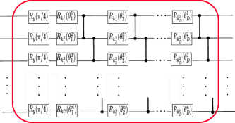
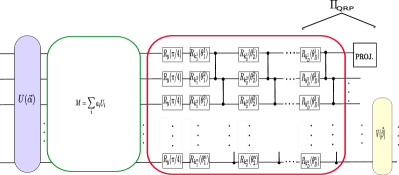
For the plots in the experiments section of the paper, we use the ansatz used in [36] which is assumed to be an exact 2-design ansatz beyond a certain depth Fig.1. The main text contains the depths at which the ansatz matches the exact 2-design limit(). There are many candidate local random circuit architectures which are approximate 2-designs [22]. Instead of studying the projection abilities of different local random circuits architecture, the appendix E contains some experiments where we look at less expensive ansatz and hence is in an approximate unitary 2- design regime by choosing a lower depth () (analogous to [34]) of the same circuit Fig. 1.
IV Experiments on quantum random Projectors
In this section, we consider two different experiments to benchmark the performance of quantum random projection discussed in the previous section against the SRHT projection which will be labeled as classical random projection in the plots. This should be looked at as a comparison of random projectors’ that can be stored and applied efficiently in terms of memory and time complexity in classical vs quantum settings. Since quantum random projectors approximate the Haar measure, their projection abilities are expected to be better than the SRHT projectors because the latter is less random compared to the Haar measure. However, in certain applications, it is known that they both converge to similar performance when the size of the data set tends to infinity [29]. We see in the appendix D that their performances start becoming closer when we increase the size of the data matrices, and vectors from 1024 to 2048 (corresponding to 10 and 11 qubits, respectively).
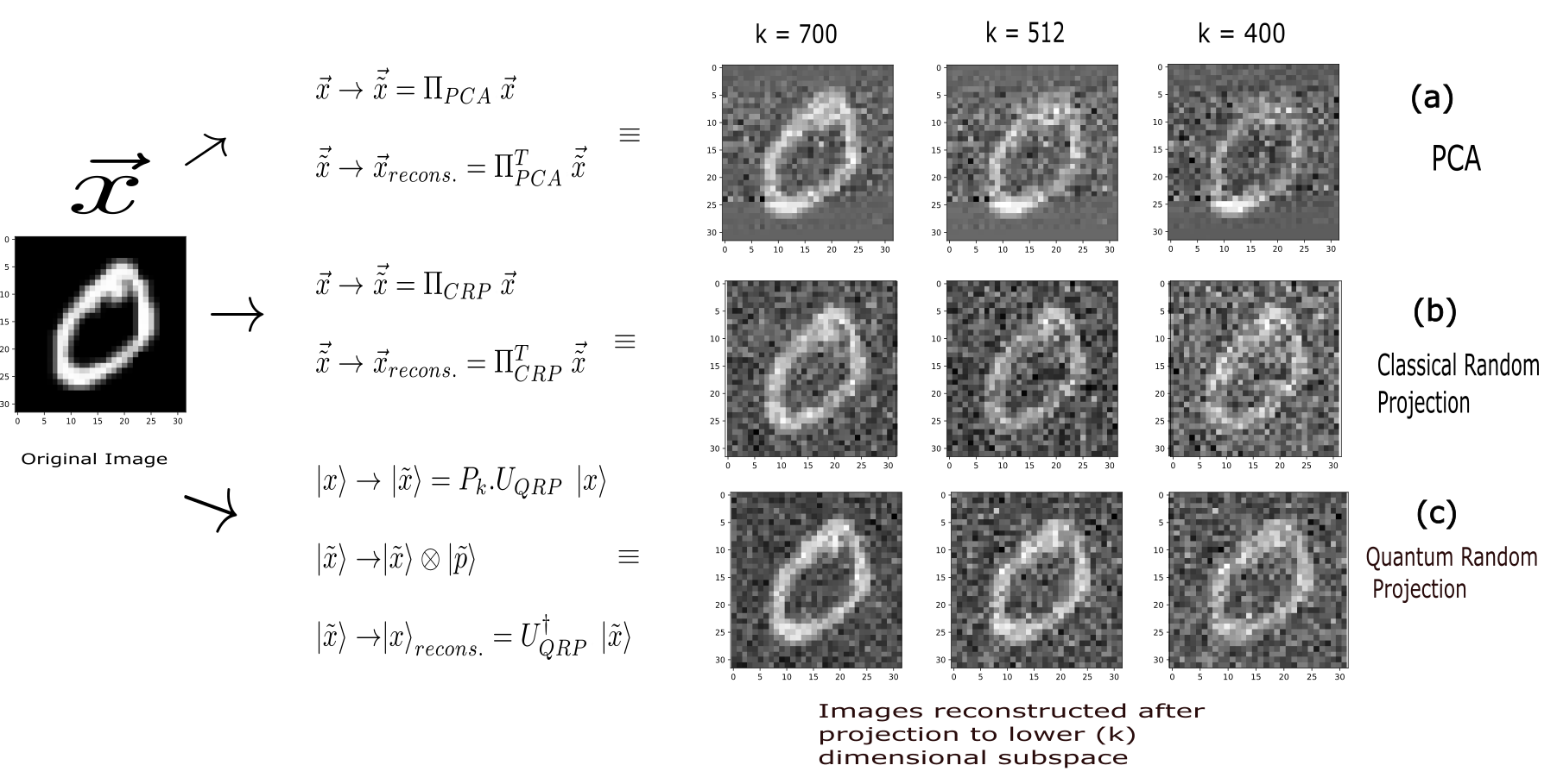
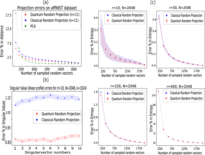
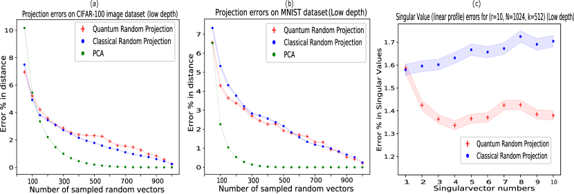
We initially consider the task that doesn’t require us to know the singular values and is concerned with only dimensionality reduction. In this regard, we reduce the dimensions of the MNIST [24] and CIFAR 100[25] image datasets and benchmark the performance of quantum random projection against classical random projection. We also compare it with the computationally expensive principal components analysis (PCA) which is supposed to give the exact projection to the dominant singular vectors of the datasets and cannot be outperformed beyond a certain rank.
In the second task, we calculate the Von Neumann entropy of low-rank density matrices (along the lines of [26]) which requires us to know the singular values after random projection in addition to the dimensionality reduction. We compare the performance of quantum random projection (QRP) vs classical random projection (CRP) for this task over different ranks (r) of the density matrices.
In this section, we pick the local random quantum circuit from Fig. 1 and we assume that we can make arbitrary projection operators with any number of basis vectors, i.e, if the operator projects to the first basis state in any basis. Then,
| (9) |
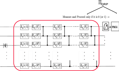
where we don’t have any restriction on what basis we pick and what values k can take. In a later section, we discuss the simplest projection operator one can construct by measuring one or more qubits and restricting to particular outputs (0 or 1) in those qubits, as shown in Fig.2. It is worth noting that this scheme has a structure similar to the quantum autoencoders ([37]) but the circuit here is data-agnostic.
IV.1 Dimensionality reduction of Image data sets
In this subsection, we benchmark the performance of the QRP against CRP in the task of dimension reduction of subsets of two different image datasets, MNIST and CIFAR-100. We also plot the performance of the computationally expensive PCA which is supposed to capture all the nonzero singular valued singular vectors. When the reduced dimension is greater than the rank of the system, PCA could never be outperformed.
MNIST contains 28x28 grayscale images. The matrix representations of the images were boosted to 32x32 so that they can be reshaped into 1024x1 normalised vectors by adding zeros(Note that this is not a common quantum encoding scheme. We use QRP on the normalized data vectors for a direct comparison with CRP). We have to do this preprocessing step because the projectors that we consider (both CRP and QRP) are of the form and hence take only dimensional vectors as the input.
CIFAR-100, in addition to being 28x28 images, are also colored images and had to be converted to 32x32 grayscale so that they can be fed as input to our projectors. But unlike MNIST, which contains handwritten integers from 0 to 9, the CIFAR-100 dataset contains images belonging to 100 different classes including Airplanes, Automobiles, birds, cats, trucks, etc. As a result, CIFAR-100 is expected to have more features in their datasets and hence greater rank compared to MNIST if we consider subsets from each of these datasets.
To perform the comparison between CRP and QRP, we took 1000 images from each of these datasets. And in each of these subsets, we reshaped the images into 1024x1 normalized vectors and performed random projection to lower dimensions (x-axis of the Fig. 3). Then, we randomly sampled two data vectors and compared the error percentage in their norm (Euclidean distance) between them in the original space and the reduced dimensional space obtained after random projection. This procedure is repeated 10,000 times and the mean error percentages and their 95 confidence intervals for different reduced dimensions has been reported in the plots Fig.3.
The random projections are performed by multiplying the vectors with random matrices (see Algorithm 1 and Algorithm 2)
| (10) | |||
| (11) |
where is the SRHT projector and , are the sampled from the matrix representation of local random quantum circuit and projectors used. And PCA projection is obtained by first computing singular value decomposition on the dataset and projecting them to the subspace of dominant singular vectors.
| (12) |
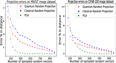
Fig.3 show that the PCA outperforms the random projection methods beyond a certain rank. This is because, beyond the rank of the dataset considered, PCA projects exactly to the subspace with non-zero singular values. Despite that, we see that random projection methods which are not computationally extensive (because they don’t compute the subspace with non-zero singular values) perform to the same extent and even better than the PCA at lower reduced dimensions. This dominance in performance at lower reduced dimensions is visible in larger dimensional datasets (see Appendix D). We also see that PCA takes more reduced dimensional vectors to catch up with the random projection algorithms in the case of CIFAR-100 because it has comparatively more rank (loosely because it has more features) than the MNIST dataset. These data vectors dimensionally reduced via quantum random projection could be used in quantum machine learning applications such as training an image recognition/classification model (See for example [38]).
Within the random projection methods, quantum random projection performs slightly better than the classical random projection mainly because Haar random matrices are more random and have tighter JL lemma bounds than the classical random projector. The performance of quantum random projectors which are away from the exact 2-design limit has been analyzed in the Appendix E by looking at shorter depths () of Fig.1 and hence lesser expressive ansatz.
The discussion in this section assumed the existence of an exact amplitude encoding scheme for the data vectors. This would require impractical depths of unless the data vectors are genuinely quantum, e.g., groundstates of a family of local Hamiltonians. However, for general data vectors like image data vectors, we do not necessarily need exact encoding. Preserving the distinctness of image data vectors to a good enough accuracy enables us to use them for many image processing applications such as recognition, and classification. In this regard, there has been substantial work on Approximate amplitude encoding. These schemes encompass approximately encoding data vectors whose amplitudes are all positive [39], real[40], and even complex data vectors[41] using shallow parametrized quantum circuits.
With the plots in Fig.3, we showed that for exactly encoded data vectors () and quantum random projected vectors ()
| (13) |
on average for pairs of images in the data set used. Here is a very small fraction of . A good approximate amplitude encoding scheme is bound to preserve this distance with minimal error, since it preserves the distinctness of the samples as well as (calling approximate encoded vectors)
| (14) |
on average. Here is a small fraction of .
With the equations Eqs.13 and 14, it is clear that even with the approximate amplitude encoding, quantum random projection would preserve the distinctness of samples (up to a perturbation of ) and be useful for image processing applications. The exact value of depends on the efficiency of the approximate encoding used.
The other alternative to circumvent the impractical depths of the exact data encoding issue is by adopting different encoding schemes. One can start by reducing the resolution of the images (equivalent to reducing the pixels), which results in reduced classical image data vector dimension (to say ) and use any other existing data encoding schemes that use qubits’ dimensions greater than but with polynomial depths(For example [42],[43]).
If is the encoding function that takes the original data vector and encodes it as a data vector of dimension . Then, to check how well the distinctness is preserved, experiments need to be run on the qubits with a quantum random projector corresponding to qubits. Mathematically, we need to check how low the following values are (on average) for two data vectors from the original dataset
| (15) |
where are reduced randomly projected encoded vectors.
In this work, we confined ourselves to experiments involving an exact encoding scheme despite impractical depths because the preservation of distance for the exact encoding scheme implies the same for the approximate encoding schemes as described earlier. Checking the preservation of distance for other encoding schemes would require knowing the exact form of encoding in Eq.15.
Just like its classical counterpart, we can also reconstruct the images back to the original size after the random projection. For classical methods (for a data vector and its reduced data vector )
| (16) | |||
| (17) |
For the quantum case, we need to put in the extra qubits or the subspace to which we projected to get back to the original size and then apply the inverse of the unitary circuit used for projection. For example, if we had projected to the subspace where one of the qubits is in state. We boost the size back to the original size by having a new qubit at and add the inverse unitary circuit () on this new system. For a general projector, where tensor product with the ensures that we get back the original size of the data(image). And the reconstruction is done as follows (For the dataset )
| (18) |
This is similar to the reconstruction done in [37]. These reconstructions work on the premise that the product of the original data dimension. It is trivial to see that this holds for the PCA projector. It turns out that this also holds for the random projectors. This is because in a larger dimensional space, finding almost orthogonal vectors becomes more common, this has been studied in [44] and was used in the discussion of [11]. Fig.4 shows how one would reconstruct an image from the MNIST dataset after dimensionally reducing a subset of the MNIST images.
With the reconstructed quantum data vectors, there are processing applications which have computational advantage over classical processing. For example, the complexity of the quantum edge detection algorithm [45] is polynomial and doesn’t require exponential resources if we have an image encoded either exactly or approximately. The measurement outputs of the edge detection algorithm contain information about the edges. To get the outputs of this experiment, one can also adopt the classical shadows [46, 47] approach to get the probabilities of all the bit strings with less number of measurements than full-state tomography.
IV.2 Entropy estimation of low-rank density matrices
In this subsection, we compare the performance of the quantum random projectors against the classical random projector, SRHT on a task that requires one to obtain the approximate singular values of the dominant singular vectors of a data matrix after the dimensionality reduction. Unlike the previous task, this is concerned with reducing the dimensions of a large data matrix instead of individual data vectors by random projection. After the dimensionality reduction, we check how well the system captures the properties of the dataset by computing the error percentage in a particular property of the data matrix which requires the knowledge of all its singular values.
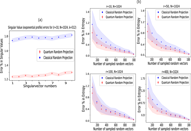
Specifically, we will consider randomly generated semi-positive definite density matrices with random singular vectors but their singular values follow a certain profile. We then compute their entropy after quantum random projection and check their accuracy(along the lines of [26]). The exact singular values profile of these density matrices depends on the nature of the system. In this experiment, we consider singular values which are linearly decaying and exponentially decaying until the rank of the system and zero afterward. These profiles could be motivated through the existence of physical systems with such profiles. A thermal ensemble of a simple harmonic oscillator mode of frequency with N internal degrees of freedom has an exponentially decaying profile. Here, singular values of will be proportional to and so on. And, it is known that maximal second order Rényi entropy ensemble of a system with a simple harmonic oscillator mode of frequency and N internal degrees of freedom follows a linearly decaying singular value profile for its density matrix [48]. The main text contains the plots related to the linearly decaying singular profile and the appendix C contains the plots related to the exponential decay profile.
Here is the procedure to perform random projection given a semi-positive definite matrix of dimension
-
•
Project the original density matrix of size to a lower dimension using and
-
•
Perform SVD (classical) or QSVD (quantum) on the lower dimensional matrix to get the singular vectors with singular values ,,,…. which are approximations to .
-
•
Then we obtain an approximation to entropy (S) using
The accuracy in the approximated entropy is bounded in the following theorem IV.1
Theorem IV.1.
For a random matrix satisfying the Johnson-Lindenstrauss (JL) lemma with a distortion , where and , the difference in the Von Neumann entropy of a density matrix computed using the random projection with (denoted as ) and the true entropy () can be bounded as follows
| (19) |
with probability at least ().
Proof.
See Appendix A.3 ∎
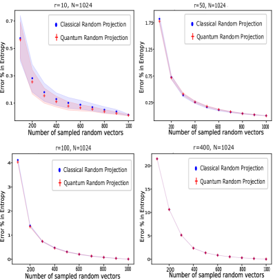
The Fig.5 shows the error percentage in the computed entropy after random projection for density matrices of size with linearly decaying singular values until a certain rank ( in the plot) and zero afterward. The x-axis represents the different reduced dimensions (). The accuracies are better for low ranks as expected and get worse for larger ranks. We observe that the quantum random Projector and the classical random projector perform to similar extents (if not a better quantum performance than classical performance for density matrices
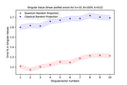
with very low rank) in this task. This matches the trends reported in [26] where they reported similar performance for various other classical random projection matrices like Gaussian, SRHT, and IST. We also show the accuracies with which the quantum and classical random projectors capture the singular values of the system for the rank when the system’s size has been reduced by half in figure 6. Here, we see that the quantum random projectors perform better than their classical counterpart mainly because Haar random matrices that the random circuits try to approximate is more random than any classical random projectors that could be stored with similar or comparable complexity. The appendix contains a discussion regarding how the accuracy improves when we increase the size of the original datasets from 1024 1024 to 2048 2048.
We discuss the same plots for density matrices with exponentially decaying singular value profile until a certain rank in the Appendix C. We observe there that increasing the rank doesn’t change the singular value profile as much and hence the accuracy with which the random projection algorithms work remains pretty much constant. The appendix E contains the error plots for the accuracy in individual singular values for the case obtained using lesser expressive random circuits (depth ).
V How to project in a real Quantum Computer?
For the quantum random projection to work, in addition to sampling a unitary from the exact (or approximate 2 designs), we also need to have a circuit component for projector operators. In one of the previous sections, we considered arbitrary projection operators which might not be able to be efficiently implemented in a quantum computer with polynomial resources. However, we can look at the simplest projection operations that one can use for the quantum random projection. In Fig.2, we looked at the simplest projection operation, which is measuring some of the qubits and proceeding only if the qubits are in a certain state ( or ). This is equivalent to projecting it to the subspace where those qubits take that specific value. For example, when you have a circuit of 10 qubits, measuring one of the qubits and proceeding only when that qubit is in means a reduction in the data vector (or ket) dimension from 1024 to 512.
However, the projection through measurement discussed above is different compared to the classical projection because a quantum measurement (wavefunction collapse) automatically takes care of the normalization factor and the extra is not needed. Since the Hilbert space we consider here is large and the ket entries are randomized, the normalization that happens because of the wavefunction is the same as the prefactor we would get in a classical random projection.
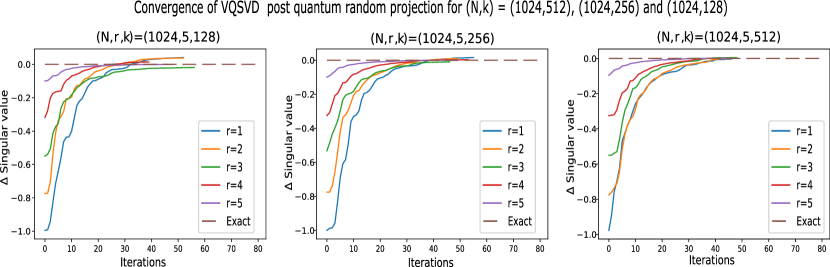
To demonstrate the quantum random projection with a simple projection operation, we will consider projection operators of the form which is a projection operator to the space where qubit is at state.To demonstrate this, we perform such a quantum random projection for a large data matrix with a linearly decaying singular values profile of size and rank by reducing the data vectors to sizes 512, 256 and 128 by projecting out 1, 2 and 3 qubits respectively. Then, we retrieve the dominant singular vectors by performing a variational quantum singular value decomposition (VQSVD)[6]. But since the data matrix has been dimensionally reduced, the ansatz we use for finding the right singular vectors is also of reduced size (Fig.7). The details regarding the implementation of VQSVD, and the ansatz type used can be found in the Appendix F.
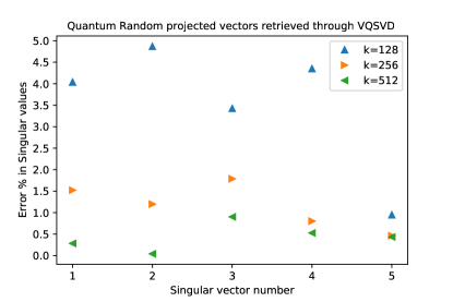
The Fig.8 shows the accuracy with which we were able to reconstruct the singular vectors after quantum random projection for individual singular vectors. This demonstrates how one can perform quantum random projection in near-term devices as the VQSVD algorithm used to retrieve the dominant vectors is a near-term algorithm. The accuracy with which the singular values have been retrieved depends on the expressivity of the ansatz and whether or not it falls into a barren plateau during the training procedure. We haven’t discussed the most accurate retrieval of the singular vectors, as that is beyond the scope of this paper. There are many strategies to avoid falling into the barren plateau and improve the convergence rate [49, 50, 51]. We used the identity block strategy [51] to avoid barren plateaus (more details on that in the appendix F.)
VI Conclusion
In this work, we explored a practically useful application of local random quantum circuits in the task of dimensional reduction of large low-rank data sets. The main essence of the applicability of the local random circuits in this task is their ability to anticoncentrate rapidly at linear or sub-linear depths [52, 53]. This makes them a good random projector to lower dimensions, meaning they preserve the distinctness of different dominant data vectors in a large dataset after dimensional reduction.
The theorems discussed in the paper show that just like the Haar random matrices which are good random projectors, their approximate quantum implementations, the exact and approximate t-designs are also good random projectors. The rapid anti-concentration of Hilbert space at linear depths means that the number of random parameters(the random rotation parameters) required to create and reproduce a random projector is logarithmic in the size of the data sets. Such efficiency in the storage complexity of classically generated Haar random matrices or in any classical random projector is not possible. We then, benchmarked its performance against the commonly used classical random projector, Subsampled Randomised Hadamard Transform (SRHT). The quantum random projectors performed slightly better than this classical candidate because they are trying to approximate Haar random matrices which are more random than the classical candidate. We then demonstrated these comparisons for various tasks such as image compression, reconstruction, retrieving the singular values of the dominant singular vectors post-dimension reduction, etc.
Though the initial discussion assumed arbitrary projection operators to arbitrary subspaces, we showed simplest projection operators and projection subspaces exist. We demonstrated this simplest quantum random projection and retrieved the dominant singular vectors post-quantum random projection via VQSVD [6]. This shows the applicability of such quantum random projections and their retrievals in near-term devices.
Dimensionality reduction facilitated by random projections as discussed in this work can also precede kernel-based variants of PCA wherein eigenvalue decomposition of the Gram matrix associated with the higher-dimensional embedding (often called kernel) is sought [54] especially if the said Gram matrix is low-rank. Beyond the precincts of classical data, such a technique can act as an effective precursor to improve the efficiency of simulation even on quantum data as has been studied in recent work [55]. The essential crux of the idea is heavily rooted on PCA but applied to quantum data wherein repeated Schmidt decomposition of the states and vectorized form of arbitrary operators are performed followed by subsequent removal of singular vectors associated with non-dominant singular values akin to PCA. The techniques explored in this work involving good random projections can be used in conjunction prior to the application of such a protocol to contract the effective space of the states/operators involved. Owing to the demonstrated near-term applicability, similar reduction can also be afforded
as a preprocessing step in a host of quantum algorithms manipulating quantum data [56] on noisy hardwares. Such protocols are of active interest to the scientific community due to their profound physico-chemical applications ranging from exotic condensed-matter physical systems like Rydberg excitonic arrays[57], modeling higher dimensional spin-graphical architectures in quantum gravity [58] and in learning theory of neural networks[59], constructing unknown hamiltonians through time-series analysis [60, 61], tomographic estimation of quantum state [62, 63], in electronic structure of molecules and periodic materials [64], quantum preparation of low energy states of desired symmetry [64, 65] or even order-disorder transitions in conventional Ising spin glass using quantum annealers [66] and quantum variants of Sherrington-Kirkpatrick model [67] to name a few.
We did an extensive comparison using deep () exact 2-design ansatz and deferred the discussion about circuits away from the exact 2-design limit to the appendix E. This is because there exist various random circuit architectures which anti concentrate just like the exact 2-design ansatz and hence could be good candidates for random projection. This could be a good starting point for future study. Also, it is worth studying and constructing quantum random projectors suited for specific applications and datasets( for example, the datasets in health care [68, 69]). It has to be noted that the results derived in the main text assumed noiseless quantum gates and measurements. Similar theorems need to be understood for real quantum computers where different noise sources are unavoidable. This leads to a possible future study to understand the extent to which the theorems in the main text are valid on real quantum computers by performing statistical analysis on the bitstrings from the output of real quantum computers (See Refs. [70, 71]).
VII Code availability
The classical and the quantum random projection matrix(and the rotation parameters used to generate the circuit) used for the comparisons, the data matrix used to generate Fig. 8 along with the code for generating the plots in this paper will be made available upon reasonable request. The simulation for the retrieval of dominant singular vectors through VQSVD was done in the Paddle quantum framework [72].
VIII ACKNOWLEDGEMENTS
We would like to acknowledge funding from the Office of Science through the Quantum Science Center (QSC), a National Quantum Information Science Research Center, the U.S. Department of Energy (DOE) (Office of Basic Energy Sciences) under award no. DE-SC0019215, and the National Science Foundation under award number 1955907.
References
- Velliangiri et al. [2019] S. Velliangiri, S. Alagumuthukrishnan, and S. I. Thankumar joseph, A review of dimensionality reduction techniques for efficient computation, Procedia Computer Science 165, 104 (2019), 2nd International Conference on Recent Trends in Advanced Computing ICRTAC -DISRUP - TIV INNOVATION , 2019 November 11-12, 2019.
- Salem and Hussein [2019] N. Salem and S. Hussein, Data dimensional reduction and principal components analysis, Procedia Computer Science 163, 292 (2019), 16th Learning and Technology Conference 2019Artificial Intelligence and Machine Learning: Embedding the Intelligence.
- Lloyd et al. [2014] S. Lloyd, M. Mohseni, and P. Rebentrost, Quantum principal component analysis, Nature Physics 10, 631 (2014).
- Rebentrost et al. [2018] P. Rebentrost, A. Steffens, I. Marvian, and S. Lloyd, Quantum singular-value decomposition of nonsparse low-rank matrices, Phys. Rev. A 97, 012327 (2018).
- Kerenidis and Prakash [2016] I. Kerenidis and A. Prakash, Quantum recommendation systems (2016), arXiv:1603.08675 [quant-ph] .
- Wang et al. [2021] X. Wang, Z. Song, and Y. Wang, Variational Quantum Singular Value Decomposition, Quantum 5, 483 (2021).
- Wossnig et al. [2018] L. Wossnig, Z. Zhao, and A. Prakash, Quantum linear system algorithm for dense matrices, Phys. Rev. Lett. 120, 050502 (2018).
- Preskill [2018] J. Preskill, Quantum Computing in the NISQ era and beyond, Quantum 2, 79 (2018).
- Drineas and Mahoney [2016] P. Drineas and M. W. Mahoney, Randnla: Randomized numerical linear algebra, Commun. ACM 59, 80–90 (2016).
- Achlioptas [2003] D. Achlioptas, Database-friendly random projections: Johnson-lindenstrauss with binary coins, Journal of Computer and System Sciences 66, 671 (2003), special Issue on PODS 2001.
- Bingham and Mannila [2001] E. Bingham and H. Mannila, Random projection in dimensionality reduction: Applications to image and textdata (2001).
- Johnson and Lindenstrauss [1984] W. Johnson and J. Lindenstrauss, Extensions of lipschitz mappings into a hilbert space. (1984).
- Paul et al. [2014] S. Paul, C. Boutsidis, M. Magdon-Ismail, and P. Drineas, Random projections for linear support vector machines (2014), arXiv:1211.6085 [cs.LG] .
- Alman and Williams [2020] J. Alman and V. V. Williams, A refined laser method and faster matrix multiplication (2020), arXiv:2010.05846 [cs.DS] .
- Ailon and Chazelle [2009] N. Ailon and B. Chazelle, The fast johnson–lindenstrauss transform and approximate nearest neighbors, SIAM Journal on Computing 39, 302 (2009), https://doi.org/10.1137/060673096 .
- Knill [1995] E. Knill, Approximation by quantum circuits (1995), arXiv:quant-ph/9508006 [quant-ph] .
- Dankert et al. [2009] C. Dankert, R. Cleve, J. Emerson, and E. Livine, Exact and approximate unitary 2-designs and their application to fidelity estimation, Phys. Rev. A 80, 012304 (2009).
- Dankert [2005] C. Dankert, Efficient simulation of random quantum states and operators (2005), arXiv:quant-ph/0512217 [quant-ph] .
- Ambainis and Emerson [2007] A. Ambainis and J. Emerson, Quantum t-designs: t-wise independence in the quantum world, in Twenty-Second Annual IEEE Conference on Computational Complexity (CCC’07) (2007) pp. 129–140.
- Harrow and Low [2009] A. W. Harrow and R. A. Low, Random quantum circuits are approximate 2-designs, Communications in Mathematical Physics 291, 257 (2009).
- Brandão et al. [2016] F. G. S. L. Brandão, A. W. Harrow, and M. Horodecki, Local random quantum circuits are approximate polynomial-designs, Communications in Mathematical Physics 346, 397 (2016).
- Haferkamp [2022] J. Haferkamp, Random quantum circuits are approximate unitary -designs in depth , Quantum 6, 795 (2022).
- Sen [2018] P. Sen, A quantum johnson-lindenstrauss lemma via unitary t-designs (2018), arXiv:1807.08779 [quant-ph] .
- Deng [2012] L. Deng, The mnist database of handwritten digit images for machine learning research, IEEE Signal Processing Magazine 29, 141 (2012).
- Krizhevsky [2009] A. Krizhevsky, Learning multiple layers of features from tiny images, Tech. Rep. (2009).
- Kontopoulou et al. [2020] E.-M. Kontopoulou, G.-P. Dexter, W. Szpankowski, A. Grama, and P. Drineas, Randomized linear algebra approaches to estimate the von neumann entropy of density matrices (2020), arXiv:1801.01072 [cs.IT] .
- Dong et al. [2022] Y. Dong, T. Gong, S. Yu, H. Chen, and C. Li, Robust and fast measure of information via low-rank representation (2022), arXiv:2211.16784 [cs.LG] .
- Ghojogh et al. [2021] B. Ghojogh, A. Ghodsi, F. Karray, and M. Crowley, Johnson-lindenstrauss lemma, linear and nonlinear random projections, random fourier features, and random kitchen sinks: Tutorial and survey (2021), arXiv:2108.04172 [stat.ML] .
- Lacotte and Pilanci [2020] J. Lacotte and M. Pilanci, Optimal randomized first-order methods for least-squares problems (2020), arXiv:2002.09488 [math.OC] .
- Drineas et al. [2011] P. Drineas, and M. Mahoney, and S. Muthukrishnan, and T. Sarlós, Faster least squares approximation }Numerische Mathematik 117, 219 (2011), copyright: Copyright 2021 Elsevier B.V., All rights reserved.
- Nelson and NguyÅn [2013] J. Nelson and H. L. NguyÅn, Sparsity lower bounds for dimensionality reducing maps (Association for Computing Machinery, New York, NY, USA, 2013).
- Tropp [2011] J. A. Tropp, Improved analysis of the subsampled randomized hadamard transform, Adv. Adapt. Data Anal. 3, 115 (2011).
- Nakaji and Yamamoto [2021] K. Nakaji and N. Yamamoto, Expressibility of the alternating layered ansatz for quantum computation, Quantum 5, 434 (2021).
- Holmes et al. [2022] Z. Holmes, K. Sharma, M. Cerezo, and P. J. Coles, Connecting ansatz expressibility to gradient magnitudes and barren plateaus, PRX Quantum 3, 010313 (2022).
- Low [2010] R. A. Low, Pseudo-randomness and learning in quantum computation (2010), arXiv:1006.5227 [quant-ph] .
- McClean et al. [2018] J. R. McClean, S. Boixo, V. N. Smelyanskiy, R. Babbush, and H. Neven, Barren plateaus in quantum neural network training landscapes, Nature Communications 9, 10.1038/s41467-018-07090-4 (2018).
- Romero et al. [2017] J. Romero, J. P. Olson, and A. Aspuru-Guzik, Quantum autoencoders for efficient compression of quantum data, Quantum Science and Technology 2, 045001 (2017).
- Lü et al. [2021] Y. Lü, Q. Gao, J. Lü, M. Ogorzałek, and J. Zheng, A quantum convolutional neural network for image classification, in 2021 40th Chinese Control Conference (CCC) (2021) pp. 6329–6334.
- Zoufal et al. [2019] C. Zoufal, A. Lucchi, and S. Woerner, Quantum generative adversarial networks for learning and loading random distributions, npj Quantum Information 5, 10.1038/s41534-019-0223-2 (2019).
- Nakaji et al. [2022] K. Nakaji, S. Uno, Y. Suzuki, R. Raymond, T. Onodera, T. Tanaka, H. Tezuka, N. Mitsuda, and N. Yamamoto, Approximate amplitude encoding in shallow parameterized quantum circuits and its application to financial market indicators, Physical Review Research 4, 10.1103/physrevresearch.4.023136 (2022).
- Mitsuda et al. [2023] N. Mitsuda, K. Nakaji, Y. Suzuki, T. Tanaka, R. Raymond, H. Tezuka, T. Onodera, and N. Yamamoto, Approximate complex amplitude encoding algorithm and its application to data classification problems (2023), arXiv:2211.13039 [quant-ph] .
- Le et al. [2011] P. Q. Le, F. Dong, and K. Hirota, A flexible representation of quantum images for polynomial preparation, image compression, and processing operations, Quantum Information Processing 10, 63 (2011).
- Zhang et al. [2013] Y. Zhang, K. Lu, Y. Gao, and M. Wang, NEQR: a novel enhanced quantum representation of digital images, Quantum Information Processing 12, 2833 (2013).
- R. [1994] H.-N. R., Context vectors: general purpose approximate meaning representations self-organized from raw data, Computational Intelligence: Imitating Life, IEEE Press , 43 (1994).
- Yao et al. [2017] X.-W. Yao, H. Wang, Z. Liao, M.-C. Chen, J. Pan, J. Li, K. Zhang, X. Lin, Z. Wang, Z. Luo, W. Zheng, J. Li, M. Zhao, X. Peng, and D. Suter, Quantum image processing and its application to edge detection: Theory and experiment, Physical Review X 7, 10.1103/physrevx.7.031041 (2017).
- Huang et al. [2020] H.-Y. Huang, R. Kueng, and J. Preskill, Predicting many properties of a quantum system from very few measurements, Nature Physics 16, 1050–1057 (2020).
- Huang et al. [2021] H.-Y. Huang, R. Kueng, and J. Preskill, Efficient estimation of pauli observables by derandomization, Physical Review Letters 127, 10.1103/physrevlett.127.030503 (2021).
- Giudice et al. [2021] G. Giudice, A. Ç akan, J. I. Cirac, and M. C. Bañuls, Rényi free energy and variational approximations to thermal states, Physical Review B 103, 10.1103/physrevb.103.205128 (2021).
- Cerezo et al. [2021] M. Cerezo, A. Sone, T. Volkoff, L. Cincio, and P. J. Coles, Cost function dependent barren plateaus in shallow parametrized quantum circuits, Nature Communications 12, 10.1038/s41467-021-21728-w (2021).
- Cerezo et al. [2022] M. Cerezo, K. Sharma, A. Arrasmith, and P. J. Coles, Variational quantum state eigensolver, npj Quantum Information 8, 10.1038/s41534-022-00611-6 (2022).
- Grant et al. [2019] E. Grant, L. Wossnig, M. Ostaszewski, and M. Benedetti, An initialization strategy for addressing barren plateaus in parametrized quantum circuits, Quantum 3, 214 (2019).
- Hangleiter et al. [2018] D. Hangleiter, J. Bermejo-Vega, M. Schwarz, and J. Eisert, Anticoncentration theorems for schemes showing a quantum speedup, Quantum 2, 65 (2018).
- Dalzell et al. [2022] A. M. Dalzell, N. Hunter-Jones, and F. G. S. L. Brandã o, Random quantum circuits anticoncentrate in log depth, PRX Quantum 3, 10.1103/prxquantum.3.010333 (2022).
- Wang [2012] Q. Wang, Kernel principal component analysis and its applications in face recognition and active shape models, arXiv preprint arXiv:1207.3538 (2012).
- Daskin et al. [2023] A. Daskin, R. Gupta, and S. Kais, Dimension reduction and redundancy removal through successive schmidt decompositions, Applied Sciences 13, 10.3390/app13053172 (2023).
- Sajjan et al. [2022a] M. Sajjan, J. Li, R. Selvarajan, S. H. Sureshbabu, S. S. Kale, R. Gupta, V. Singh, and S. Kais, Quantum machine learning for chemistry and physics, Chem. Soc. Rev. 51, 6475 (2022a).
- Sajjan et al. [2022b] M. Sajjan, H. Alaeian, and S. Kais, Magnetic phases of spatially modulated spin-1 chains in rydberg excitons: Classical and quantum simulations, The Journal of Chemical Physics 157 (2022b).
- Borissov et al. [1996] R. Borissov, S. Major, and L. Smolin, The geometry of quantum spin networks, Classical and Quantum Gravity 13, 3183 (1996).
- Sajjan et al. [2023] M. Sajjan, V. Singh, R. Selvarajan, and S. Kais, Imaginary components of out-of-time-order correlator and information scrambling for navigating the learning landscape of a quantum machine learning model, Physical Review Research 5, 013146 (2023).
- Gupta et al. [2023] R. Gupta, R. Selvarajan, M. Sajjan, R. D. Levine, and S. Kais, Hamiltonian learning from time dynamics using variational algorithms, The Journal of Physical Chemistry A 127, 3246 (2023).
- Yu et al. [2023] W. Yu, J. Sun, Z. Han, and X. Yuan, Robust and efficient hamiltonian learning, Quantum 7, 1045 (2023).
- Gupta et al. [2022] R. Gupta, M. Sajjan, R. D. Levine, and S. Kais, Variational approach to quantum state tomography based on maximal entropy formalism, Physical Chemistry Chemical Physics 24, 28870 (2022).
- Gupta et al. [2021] R. Gupta, R. Xia, R. D. Levine, and S. Kais, Maximal entropy approach for quantum state tomography, PRX Quantum 2, 010318 (2021).
- Sajjan et al. [2021] M. Sajjan, S. H. Sureshbabu, and S. Kais, Quantum machine - learning for eigenstate filtration in two - dimensional materials, Journal of the American Chemical Society 143, 18426 (2021).
- Selvarajan et al. [2022] R. Selvarajan, M. Sajjan, and S. Kais, Variational quantum circuits to prepare low energy symmetry states, Symmetry 14, 457 (2022).
- Yaacoby et al. [2022] R. Yaacoby, N. Schaar, L. Kellerhals, O. Raz, D. Hermelin, and R. Pugatch, Comparison between a quantum annealer and a classical approximation algorithm for computing the ground state of an ising spin glass, Phys. Rev. E 105, 035305 (2022).
- Schindler et al. [2022] P. M. Schindler, T. Guaita, T. Shi, E. Demler, and J. I. Cirac, Variational ansatz for the ground state of the quantum sherrington-kirkpatrick model, Physical Review Letters 129, 220401 (2022).
- Mirniaharikandehei et al. [2020] S. Mirniaharikandehei, M. Heidari, G. Danala, S. Lakshmivarahan, B. Z. S. of Electrical, C. Engineering, U. of Oklahoma, Norman, Ok, Usa, and S. of Physical Sciences, Applying a random projection algorithm to optimize machine learning model for predicting peritoneal metastasis in gastric cancer patients using ct images, Computer methods and programs in biomedicine 200, 105937 (2020).
- Heidari et al. [2020] M. Heidari, S. Lakshmivarahan, S. Mirniaharikandehei, G. Danala, S. K. R. Maryada, H. Liu, B. Zheng, S. of Electrical, C. Engineering, U. of Oklahoma, Norman, Ok, Usa, and S. of Physical Sciences, Applying a random projection algorithm to optimize machine learning model for breast lesion classification, IEEE Transactions on Biomedical Engineering 68, 2764 (2020).
- Oh and Kais [2023] S. Oh and S. Kais, Comparison of quantum advantage experiments using random circuit sampling, Phys. Rev. A 107, 022610 (2023).
- Oh and Kais [2022] S. Oh and S. Kais, Statistical analysis on random quantum circuit sampling by sycamore and zuchongzhi quantum processors, Physical Review A 106, 10.1103/physreva.106.032433 (2022).
- Pad [2020] Paddle Quantum (2020).
- Woodruff [2014] D. P. Woodruff, Computational advertising: Techniques for targeting relevant ads, Foundations and Trends® in Theoretical Computer Science 10, 1 (2014).
- Kandala et al. [2017] A. Kandala, A. Mezzacapo, K. Temme, M. Takita, M. Brink, J. M. Chow, and J. M. Gambetta, Hardware-efficient variational quantum eigensolver for small molecules and quantum magnets, Nature 549, 242 (2017).
Appendix A Proofs of theorems in the main text
Theorem A.1.
(Theorem III.1 in main manuscript) Let be sampled uniformly from the Haar measure() and let , . Then the matrix obtained by considering any k rows of followed by multiplication with satisfy
| (20) |
with probability greater than with being the error threshold.
Proof.
Let be the projector operator to any k basis states of the Hilbert space. Without loss of generality, let us consider to be of unit norm. The components of such will be such that .Then,
| (21) |
where are k components of the vector depending on the ’s projection subspace. Then,
| (22) |
because we know that the Haar measure satisfies the translational invariance
| (23) |
when V is an element belonging to the group. By choosing to be the matrix that switches -th and -th components of an -dimensional complex vector, we get the required relation Eq. 22. Now using the fact that is unit norm, we get
| (24) |
Now, to show that sampling from the Haar measure produces a low distortion () with a very high probability, we should look at the variance of the projected norm. We should essentially show that with a very high probability. Consider Variance
| (25) | |||
| (26) |
We know that the Haar measure and quantum circuits which are 2-designs (with ) depth anti concentrate ([52, 53]). Specifically for Haar measure at large N, we have
| (27) |
Using , we get
| (28) |
Then, similar to our previous arguments, we can show that
| (29) |
and
| (30) |
and . (Eqs. 29,30) can be proved by using V in Eq.23 to be basis switch and basis switch. Eqs. 29,30 allows us to write Eq.26 as,
| (31) |
The variance for the would be which scales as for large . Using the derived variance and the deviation from the mean to be gives (using Chebysev’s inequality)
| (32) |
∎
Theorem A.2.
(Theorem III.2 in main manuscript) Let be sampled uniformly from the approximate unitary 2- design () and let , . Then the matrix obtained by considering any k rows of followed by multiplication with satisfy
| (33) |
with a probability greater than with being the error threshold.
Proof.
Define a function
| (34) |
Let be defined as follows
| (35) | |||
| (36) |
In terms of we can write Eq. 26 and Eq.36 as
| (37) |
| (38) |
Then,
| (39) |
| (40) |
where we used the monomial definition of approximate unitary 2-designs and its equivalence (See [35]) to the diamond norm definition used in the main text. Using the theorem A.1, we get
| (41) |
The variance for the would be greater than which scales as for large . Using the derived variance (upper bound from Eq.40) and the deviation from the mean to be gives (using Chebysev’s inequality )
| (42) |
∎
Theorem A.3.
(Theorem IV.1 in main manuscript) For a random matrix satisfying the Johnson-Lindenstrauss (JL) lemma with a distortion , where and , the difference in the Von Neumann entropy of a density matrix computed using the random projection with (denoted as ) and the true entropy () can be bounded as follows
| (43) |
with probability at least ().
To prove the theorem we will need to use theorems 10 and 13 of [26]. According to theorem 13, let DAD be a symmetric positive definite matrix such that D is a diagonal matrix and for all . Also, let DED be a perturbation matrix such that . Now, let be the -th eigenvalue of DAD and let be the eigenvalue of D(A+E)D. Then,
| (44) |
Now, consider a distribution on matrices (or if data vectors get multiplied from the right) satisfying
| (45) |
then, according to theorem 13 of [73], for any orthonormal matrix with rows
| (46) |
Having these two results, we can derive the bounds on the accuracy of entropy computed post-random projection. In this regard, let us look at a general semi-positive definite density matrix which could be written as where has orthonormal columns and is a diagonal matrix containing the singular values of . We note that the eigenvalues of are equal to the eigenvalues of the diagonal matrix . Similarly, the eigenvalues of are equal to the eigenvalues of . Now, using the Eq.44, we can compare the eigenvalues of the matrices
Using in the Eq. 46, we get that
| (47) |
with a probability greater than .
The eigenvalues of are equal to for and the eigenvalues of the are equal to , where are the singular values of . These are exactly equal to the singular values of . This along with Eqs.47,44 leads us to conclude:
| (48) |
This result guarantees that the singular values of (from the main text) are captured with a perturbative factor of . Using this, we can find bounds to the error in the entropy computed after the random projection. We start with the upper bound
In the second to last inequality, we used for any , and in the last inequality we used for . Similarly, we can find the lower bound to be
Combining both that bounds we get the bound for the error in entropy obtained after random projection wrt true entropy
| (49) |
Appendix B Image reconstruction post-quantum random projection
The figure 4 was a demonstration of the reconstruction of one image vector of the dataset. Since the dimensionality reduction is for the dataset as a whole, here we attach the plot of average for all the image vectors (the subset of MNIST containing 1000 images) and their reconstructed vectors in Fig.9 for various reduced dimensions along with their confidence intervals.
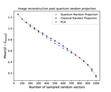
The average norm of the difference between any two unit norm vectors in 1024 dimensional space is . This sets a standard to compare the average norms plotted in the 9.
As mentioned in the experiments section, we assume that we can make arbitrary projection operators with any number of basis vectors, i.e, if the operator projects to the first basis state in any basis. Then,
| (50) |
where we don’t have any restriction on what basis we pick and what values k can take. Quantum projectors are easy to construct when k takes values 128,256 and 512 (corresponding to measuring 1,2 and 3 qubits respectively). Though it is impractical to construct such quantum projection operators for , we used those values only to compare the performance of quantum random projection against classical random projection which doesn’t have any restrictions on the values can take.
For the specific numbers mentioned in the figure, we used the first 400 and 700 components of the wave vector after the random quantum circuit () and added extra basis states with zero amplitudes to make them 1024 dimensional. Then, the wavevectors are reconstructed by the action of the inverse of i.e., . We understand that this process is more insightful when the projection operators are just 1,2 or 3 qubit measurements to specific states ( or ). There, if the quantum random projection is made such that one of the qubits is projected to say state. Then, reconstruction is done by appending the circuit to the reduced quantum state + measured qubit in (This is equivalent to adding zeros to the basis elements where the measured qubit is in state just like how we boosted dimensions from k=400 or 700 to 1024.)
Appendix C Performance of quantum random projection on exponential decay profile
Appendix D Performance of quantum random projection on larger datasets
Appendix E Performance of quantum random projection constructed using lesser expressive local random quantum circuits
Appendix F Details regarding the VQSVD performed to retrieve the dominant singular vectors
The variational quantum singular value decomposition was used to retrieve the dominant singular vectors of a randomly generated data matrix with rank () and singular values following a linearly decaying profile. The matrix on which one has to perform quantum random projection and quantum SVD needs to be loaded as a sum of unitaries or Pauli strings (unit depth). This process has exponential complexity for an exact representation of the matrix. But with importance sampling (as mentioned in the [6]) one only uses a subset of Pauli strings which approximates the matrix to sufficient accuracy. However, for our computation, just like the exact encoding scheme, we used the exact matrix. The demonstration of accurately retrieving the Singular vectors implies the same when the importance sampling creates the matrix with high accuracy.
Since, the system size we used for this variational algorithm is large, we had to use the block initialisation strategy discussed in Ref.[51] with two identity blocks in our training ansatz to avoid the barren plateau issue [36]. Each block used in our ansatz has a hardware efficient ansatz circuit [74] of depth 25 followed by it’s inverse circuit (this part will remain an inverse circuit only at the beginning of the training. During training, the parameters of these two parts update independently) to start the training procedure close to identity and hence avoid the barren plateau. The accuracies with which we retrieved the singular values and the dominant singular vectors could also be improved with other ansatze which avoid barren plateau.
The projection operators in the figure are just measurements of certain qubits and making sure they are in a certain state () or operators of the form which projects to state of qubit .