Transfer Learning for Microstructure Segmentation with CS-UNet: A Hybrid Algorithm with Transformer and CNN Encoders

Abstract

Transfer learning improves the performance of deep learning models by initializing them with parameters pre-trained on larger datasets. Intuitively, transfer learning is more effective when pre-training is on the in-domain datasets. A recent study by NASA has demonstrated that the microstructure segmentation with encoder-decoder algorithms benefits more from CNN encoders pre-trained on microscopy images than from those pre-trained on natural images. However, CNN models only capture the local spatial relations in images. In recent years, attention networks such as Transformers are increasingly used in image analysis to capture the long-range relations between pixels. In this study, we compare the segmentation performance of Transformer and CNN models pre-trained on microscopy images with those pre-trained on natural images. Our result partially confirms the NASA study that the segmentation performance of out-of-distribution images (taken under different imaging and sample conditions) is significantly improved when pre-training on microscopy images. However, the performance gain for one-shot and few-shot learning is more modest with Transformers. We also find that for image segmentation, the combination of pre-trained Transformers and CNN encoders are consistently better than pre-trained CNN encoders alone. Our dataset (of about 50,000 images) combines the public portion of the NASA dataset with additional images we collected. Even with much less training data, our pre-trained models have significantly better performance for image segmentation. This result suggests that Transformers and CNN complement each other and when pre-trained on microscopy images, they are more beneficial to the downstream tasks.

1 Introduction

Microscopy imaging provides real information about matters, but retrieving quantitative information on morphology, size, and distribution requires manual measurements on micrographs, which is not only time-consuming and labor-intensive but also prone to biases. The length and time scales of material structures and phenomena differ significantly among the components, which adds to the complexity. Creating connections between process, structure, and properties is thus a challenging problem [1, 2].

Deep Learning (DL) has been widely applied to complex systems because of its ability to extract important information automatically. Researchers have applied DL algorithms to image analysis to identify structures and to determine the relationship between microstructure and performance. DL has been demonstrated to complement physics-based methods for materials design. However, DL requires large amount of training data while the limited number of microscopy images tends to reduce its effectiveness. Learning techniques, such as transfer learning, multi-fidelity modeling, and active learning, were developed to make DL applicable to smaller datasets [2, 3]. Transferring learning uses the parameters of a model pre-trained on a larger dataset to initialize a model trained on a smaller dataset for a downstream task. For example, a Convolutional Neural Network (CNN) pre-trained on natural images can be used to initialize a neural network for image segmentation to improve its precision and reduce the training time.

Pre-training with natural images such as ImageNet is not ideal since the models trained on natural images identify high-level features that do not exist in microscopy images. Recent work by Stuckner et al. [1] demonstrated the advantage of pre-training CNN with a microscopy dataset called MicroNet that has over 110,000 images. They evaluated pre-trained CNN encoders for segmenting microscopy images of nickel-based superalloys (Super) and environmental barrier coatings (EBCs). Pre-training with MicroNet resulted in significantly higher accuracy measured in Intersection over Union (IoU) for one-shot and few-shot learning and for out-of-distribution images that have different compositions, etching, and imaging conditions than the training images.

In recent years, attention-based neural networks called Transformers are widely adopted in computer vision. While CNN extracts features from local regions of images using convolution filters to capture the spatial relation between the pixels, Transformer divides an image into patches and feeds them into a Transformer-based encoder to capture the long-range relation between pixels across the images [4, 5]. Thus, it is possible that a combination of CNN and Transformer may be more effective in transfer learning than either of the models alone.

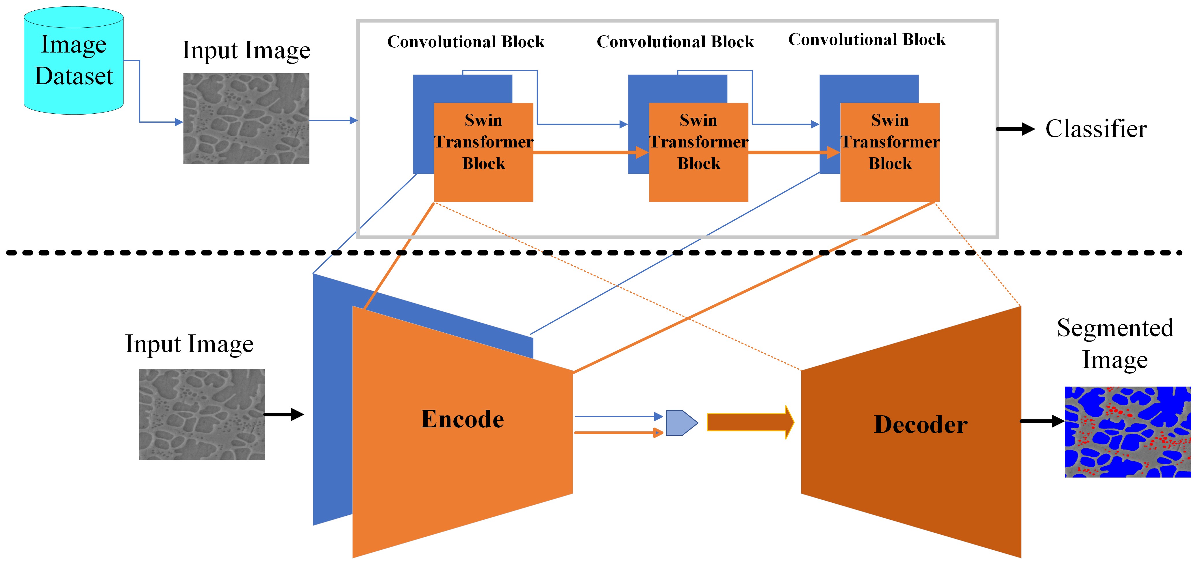
Figure 1: The encoder-decoder architecture for microstructure segmentation with transferring learning, where the CNN and Swin-T models are pre-trained on ImageNet and microscopy images. The weights of the pre-trained CNN and Swin-T models are used to initialize the encoders while the weights of the Swin-T models are used to initialize the decoders.

In this paper, we evaluate transfer learning using a combination of CNN and Transformer encoders for the segmentation of microscopy images. The transfer learning approach is illustrated in Figure 1, which contains an encoder-decoder architecture for image segmentation. Each encoder transforms the input image into a latent representation vector to extract semantic information. The decoder maps the extracted information back to each pixel in the input image to generate a pixel-wise classification of the image [1, 2, 6].

We use a popular version of Transformer – Swin-Transformer and specifically its tiny version – Swin-T[7] for efficiency purpose. Our pre-training dataset contains about 50,000 microscopy images in 74 classes, which we will refer to as MicroLite dataset. The Swin-T model can be initialized with weights from a model pre-trained on ImageNet before fine-tuned on MicroLite. We used CNN model pre-trained on MicroNet to initialize the weights of the blue encoder in Figure 1 while the Swin-T model is used to initialize the weights of the orange encoder and decoder. The output of the CNN and Swin-T encoders are fused before connecting to the decoder. To evaluate the segmentation performance with transfer learning, we compared the IoU scores of image segmentation on 7 datasets (subsets of Super and EBC) using models pre-trained on ImageNet alone and the models pre-trained on microscopy images. Our results show that while the segmentation accuracy of one-shot and few-shot learning is improved, the gain is not as large as demonstrated in the NASA paper [1]. The accuracy for out-of-distribution images remains significantly better with pre-training on microscopy images. We also compared the performance of segmentation using CNN, Swin-T, and their combination. Our results show that the combination is better than CNN alone in most cases and is better than Swin-T alone in some of the cases.

2 Related Work

In this section, we review prior research related to Transformers for image analysis and the Transformer-based segmentation algorithm that we have deployed and evaluated.

2.1 Transformer

CNN is based on the convolution operator to provide translational equivariance. However, the local receptive field of CNN limits its ability to capture long-range relation between pixels [5]. Transformer has recently been used for CV tasks as a alternative to CNN. Transformer is a type of deep neural network introduced by Vaswani et al. [8], which was successfully applied in Natural Language Processing (NLP) due to their ability to capture long-range dependencies in sequential data such as text. This approach led to significant improvements in NLP applications, such as language translation, text classification, and text generation. Compared to NLP tasks, using Transformer-based models on computer vision tasks is more challenging since images have size variations, noises, and redundant modalities. Self-attention process is the fundamental building block of Transformer aiming to learn self-alignment that provides the ability to capture the long-range relation between image patches [5]. This has led to much interest in the Transformer-based approach in CV domains [4] such as image recognition, image segmentation [9], object detection [10, 11], image super-resolution, and image generation [12].

Dosovitskiy et al. [4] proposed a Vision Transformer (ViT) based on a vanilla Transformer Network for NLP [8] with as few modifications as possible to capture the global context of an input image. ViT splits each image into patches and provides the Transformer with the linear embedding of each patch in order. Image patches are handled in the same manner as tokens in an NLP application. Supervised learning is used to train the model for image classification. The model is fine-tuned using downstream recognition benchmarks such as ImageNet classification after pre-training on a JFT dataset with 300 million images [13]. ViT has better performance than traditional CNN and achieved 88.5% on ImageNet classification task. However, ViT required more computational resources to train. In addition, the complexity of computing SoftMax for each self-attention block is quadratic with respect to the length of input sequence, limiting its applicability to high-resolution images [4, 5].

To improve a Transformer model to capture local information, Liu et al. [7] proposed a new vision Transformer called Shifted Window Transformer (Swin Transformer). This method proposed a new general-purpose backbone for image classification and recognition tasks and achieved state-of-the-art performance. The model used a shifted-window scheme to capture large variations in the scale of visual entities and high resolutions pixels in an image with linear computation complexity to input image size. In contrast, ViT [4] model produces feature maps of a single low resolution and have quadratic computation complexity to input image size because self-attention is applied globally to all the patches. Swin Transformer achieves a good performance of 87.3% on the ImageNet classification task, 58.7% box average precision score on COCO detection task, and 53.5% mIoU on the ADE20K dataset for segmentation task. The authors [7] have proposed a new version of Swin Transformer V2 that would scale it up to 3 billion parameters and allow it to train with images as high quality as $1,536\times 1,536$ pixels. Swin Transformer V2 [14] modified the Swin attention module[7] for better window resolution and scale model capacity. This is done by replacing the pre-norm with post-norm configuration, using scaled cosine attention instead of dot product attention, and replacing the previous parameterized approach with a log-spaced continuous relative position bias approach [14].

2.2 Segmentation

Ronneberger et al. [15, 16] proposed a Fully Convolutional Network (FCN) called U-Net. U-Net is a symmetric, U-shaped, encoder-decoder neural network for semantic image segmentation. U-Net consists of a typical downsampling encoder and upsampling decoder structure and a “skip connection” between them. These connections copy feature maps from the encoder and concatenate them with the feature maps in the decoder.

Xie et al. [17] proposed a semantic segmentation framework called SegFormer that combines Transformers with a lightweight multilayer perceptron (MLP) decoder. SegFormer is based on an encoder-decoder architecture, where the encoder is a hierarchically structured Transformer that outputs multi-scale features without the need for positional encoding and the lightweight All-MLP decoder aggregates the information from different layers and combines local and global attention to produce the final semantic segmentation mask. SegFormer uses a patch size of $4\times 4$ pixels to output a segmentation map. This approach helps improve dense prediction tasks and has resulted in impressive mIoU scores of 50.3% on the ADE20K dataset and 84% on the Cityscapes dataset.

Chen et al. [18] proposed TransUNet, a U-shaped architecture that employs a hybrid CNN-Transformer encoder followed by multiple up-sampling layers in the CNN-decoder. This method leverages both detailed high-resolution spatial information from CNN features and the global context encoded by Transformers. The TransUNet architecture includes 12 Vision Transformer (ViT [4]) layers in the encoder, which encode tokenized image patches obtained from CNN layers. These encoded features are then upsampled using up-sampling layers in the decoder to generate the final segmentation map, with skip-connections incorporated. TransUNet achieved high performance compared with CNN-based models.

Cao et al. [19] proposed a UNet-like pure transformer model called Swin-Unet for medical image segmentation. Swin-UNet has a U-shaped encoder-decoder architecture with skip-connections for local-global semantic feature learning by feeding the tokenized image patches into the Swin-UNet model. Both encoder and decoder structures are inspired by a hierarchical Swin-Transformer [7] with shifted windows.

Hatamizadeh et al. [20] proposed UNEt TRansformer (UNETR) model, a U-shaped encoder-decoder architecture that uses a ViT [4] as an encoder to capture global multi-scale information. The Transformer encoder is connected with the CNN-decoder using skip connections to compute the final semantic segmentation output. The proposed method has excellent accuracy and efficiency in various medical datasets for image segmentation tasks. Hatamizadeh et al.[21] also proposed a novel model for medical image segmentation of brain tumors using multi-modal MRI images. This model is called Swin UNETR. It uses the Swin Transformer [7] as encoder and connects to a CNN-based decoder via skip connections at different resolutions. In BraTS 2021 segmentation challenge, the team showed that the proposed model for multi-modal 3D brain tumor segmentation ranked among the top-performing approaches in the validation phase.

Heidari et al. [22] proposed HiFormer that bridges a CNN and a Transformer for medical image segmentation. HiFormer efficiently uses two multi-scale feature representations and a Double-Level Fusion (DLF) module to fuse global and local features. Extensive experiments show that HiFormer outperforms other CNN-based, Transformer-based, and hybrid methods in terms of computational complexity and quality of results. HiFormer provides an end-to-end training strategy that integrates global contextual representations from Swin Transformer and local representative features from the CNN module in the encoder, followed by a decoder that outputs the final segmentation map.

Azad et al. [23] proposed a novel approach, TransDeepLab, which is a DeepLabV3+ architecture based on pure Transformer for medical image segmentation. The proposed model uses a hierarchical Swin-Transformer with shifted windows to model the Atrous Spatial Pyramid Pooling (ASPP) module. The encoder module splits the input image into patches and applies Swin-Transformer blocks to encode local semantic and long-range contextual representation. A pyramid of Swin-Transformer blocks with varying window sizes is designed for ASPP to capture multi-scale information. The extracted multi-scale features are then fused into the decoder module using a Cross-Contextual attention mechanism. Finally, in the decoding path, the extracted multi-scale features are up-sampled and concatenated with the low-level features from the encoder to refine the feature representation.

The hybrid architectures mentioned in this section mainly focus on replacing CNN with a Transformer in the encoder, such as UNETR and Swin UNETR, or stacking CNN with a Transformer to form a new encoder in a sequential manner, such as Transnet [24, 25].

Replacing CNN with a Transformer in the encoder gives the strength of the ability to model long distance dependency in the network. However, it results in a lack of detailed texture feature extraction due to the removal of CNNs in the encoder. Stacking CNN with a Transformer to form a new encoder fails to account for the complementary relationship between the global modeling capability of self-attention and the local modeling capability of convolution. Instead, they treat the convolutional operation and self-attention as two separate and unrelated operations [26, 24].

To overcome these drawbacks, the encoder in CS-Unet uses CNN and Transformer in parallel to obtain rich feature information from microscopy images. CNN is used to extract low-level features and Swin-T is used to extract global contextual features, which are then fused using skip connections to the decoder at different stages/layers. Moreover, to reduce feature loss in the transmission process and increase the contextual information extracted by the Swin-T encoder, the Multi-Layer Perceptron (MLP) in two successive Swin-T blocks was replaced by Residual Multi-Layer Perceptron (ResMLP).

3 Methodology

Our objective is to demonstrate that Transformer-based pre-training models of microscopy images are beneficial to downstream tasks such as image segmentation and that they are more robust than CNN-based pre-training models. To this end, we completed the following tasks.

1. We collected a microscopy dataset with about 50,000 images after pre-processing (MicroLite),

2. We pre-trained Transformer encoders on MicroLite and used them to initialize the parameters of several Transformer-based segmentation algorithms (Swin-Unet, TransDeeplabv3+, and HiFormer) and a hybrid segmentation neural network based on CNN and Transformer encoders (CS-UNet),

3. To demonstrate the advantage of CS-UNet, we compared the top performance of CNN-based segmentation algorithms [1] with Transformer-based segmentation algorithms and CS-UNet. These algorithms are compared using the 7 test sets of the NASA team [1], where the CNN encoders are pre-trained on MicroNet [1] and Transformer encoders are pre-trained on MicroLite.

4. To evaluate the advantage of pre-training on in-domain data, we compared the top performance of CS-UNet when it is pre-trained on ImageNet and MicroLite.

5. To examine the detailed effects of pre-training on in-domain data, we compared the average performance of CNN-based segmentation algorithms with different pre-training settings. Similarly, we compared the average performance of Transformer-based and hybrid segmentation algorithms with different pre-training settings and Transformer architectures.

6. Finally, to illustrate the robustness of our hybrid strategy, we compared the performance of the three types of segmentation algorithms averaged over all configurations.

3.1 Dataset Pre-processing

The images in our MicroLite dataset are collected from multiple sources including images from different materials and compounds using various measurement techniques such as light microscopy, SEM, TEM, and X-ray. MicroLite aggregates the Aversa dataset [27], UltraHigh Carbon Steel Micrograph [28], SEM images from the Materials Data Repository, and the images from the authors of some recent publications [29, 30, 31, 32, 33, 34, 35, 36].

The Aversa dataset includes over 25,000 SEM microscopy images in 10 classes, where each class consists of images in different scales (including 1, 2, 10, 20 um and 100, 200 nm) and contrast. To properly classify these images, we used a pre-trained VGG-16 model to extract feature maps from these images and used a K-means algorithm to cluster the feature maps so that images with similar feature maps are grouped in the same class. After the pre-processing step, we obtained 53 classes. The authors of Aversa dataset manually classified a small set of the images (1038) into a hierarchical dataset where the 10 classes are further divided into 27 subclasses [27]. Our classification of these 1038 images is largely consistent with the manually assigned subclasses. Note that we have more classes since we processed the entire Aversa dataset.

In total, MicroLite includes 50,000 microscopy images labelled in 74 classes, which are obtained using the following pre-processing steps.

1. Remove any artifacts such as scale bars from the images.

2. Split the images into $512\times 512$-pixel tiles with or without overlapping depending on the size of the original images.

3. Apply data augmentation to increase the size of the dataset.

4. Aggregate the original image, the images tiles, and the augmented images to form the final dataset.

3.2 Pre-training

We trained Swin Transformers on microscopy images to learn feature representation so that it can be transferred to tasks such as segmentation. We evaluated two types of training.

1. Fine-tune a model pre-trained on ImageNet with MicroLite (denoted by ImageNet → MicroLite).

2. Pre-train a model with MicroLite from scratch (denoted by MicroLite).

The classification tasks uses Swin-T, which is the tiny version of the Swin Transformer. Swin-T consists of two types of architectures: the original Swin-T with [2,2,6,2] transformer blocks and the intermediate network with [2,2,2,2] transformer blocks. Figure 2 shows the original architecture of Swin-T. We speculate that intermediate network may be enough for microscopy analysis tasks since the earlier layers learn corner edges and shapes, the intermediate layers learn the texture or patterns, and deeper network layers in the original models learn the high-level features such as eyespots and caudal appendages. The original and intermediate Swin-T models were pre-trained on MicroLite from scratch, where the model weights are randomly initialized. The two models were also pre-trained on ImageNet and fine-tuned on MicroLite.

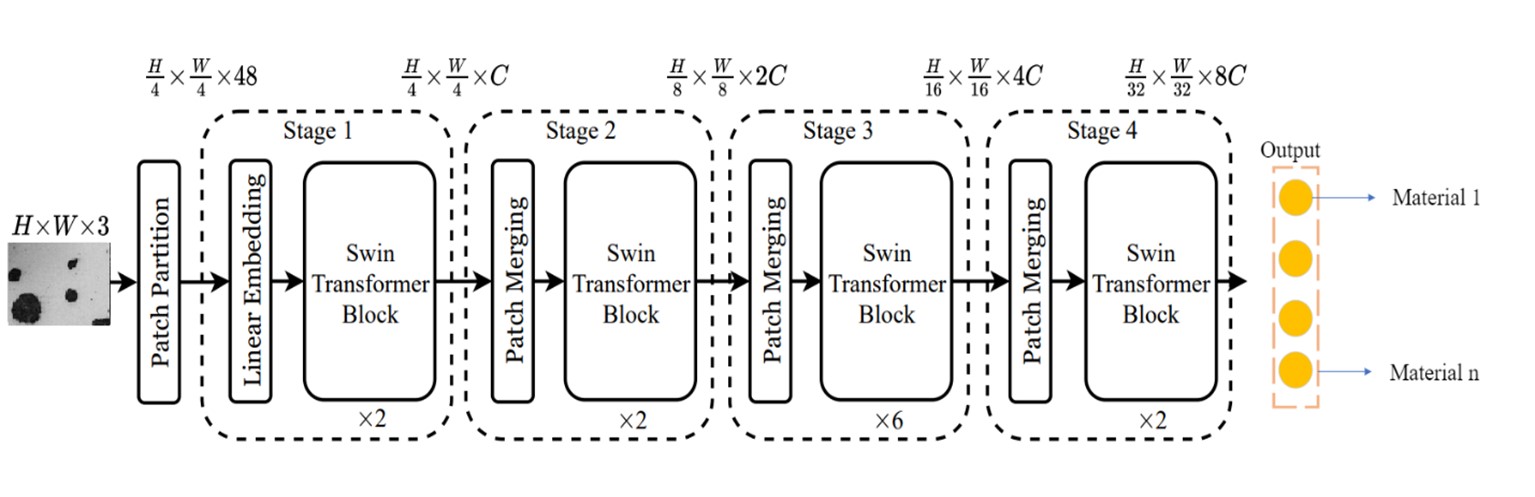
Figure 2: The original Swin-T architecture consists of four stages. Each stage contains two Swin transformer blocks except the stage three that contains six Swin transformer blocks [7]

The pre-training step uses an AdamW optimizer for 30 epochs with a cosine-decay learning-rate scheduler with 5 epochs of linear warm-up and batch size of 128. The initial learning rate is $10^{-3}$ and weight decay is $0.05$. The fine-tuning step also uses an AdamW optimizer for 30 epochs with a batch size of 128 but the learning rate is reduced to $10^{-5}$ and the weight decay is reduced to $10^{-8}$. Models were trained until there was no improvement to the validation score using an early stopping criterion with a patience of 5 epochs. Training data had been augmented using albumentations library, which included random changes to the contrast and the brightness, vertical and horizonal flips, photometric distortions, and added noise.

For the down-stream segmentation tasks, several models were trained for each task, which include Swin-Unet, HiFormer, and TrasDeeplapv3+. A comparative analysis was performed on the results of these models that were pre-trained with ImageNet and microscopy images.

3.3 Combine CNN with Transformer (CS-UNet)

CNN does not capture long-range spatial relation due to its intrinsic locality. Transformer was introduced to overcome this limitation. However, Transformer has limitations in capturing low-level features. It was shown that both local and global information are essential for dense prediction tasks such as segmentation in challenging context. Some researchers introduced hybrid models that efficiently bridge a CNN and a Transformer for image segmentation. Initializing the weights of CNN and Transformer in the hybrid models will significantly improve the performance. Therefore, we introduce a hybrid UNet called CS-UNet, which is a U-shaped segmentation model that uses both CNN and Transformer. As shown in Figure 3 , the method consists of encoder, bottleneck, decoder, and skip connections.

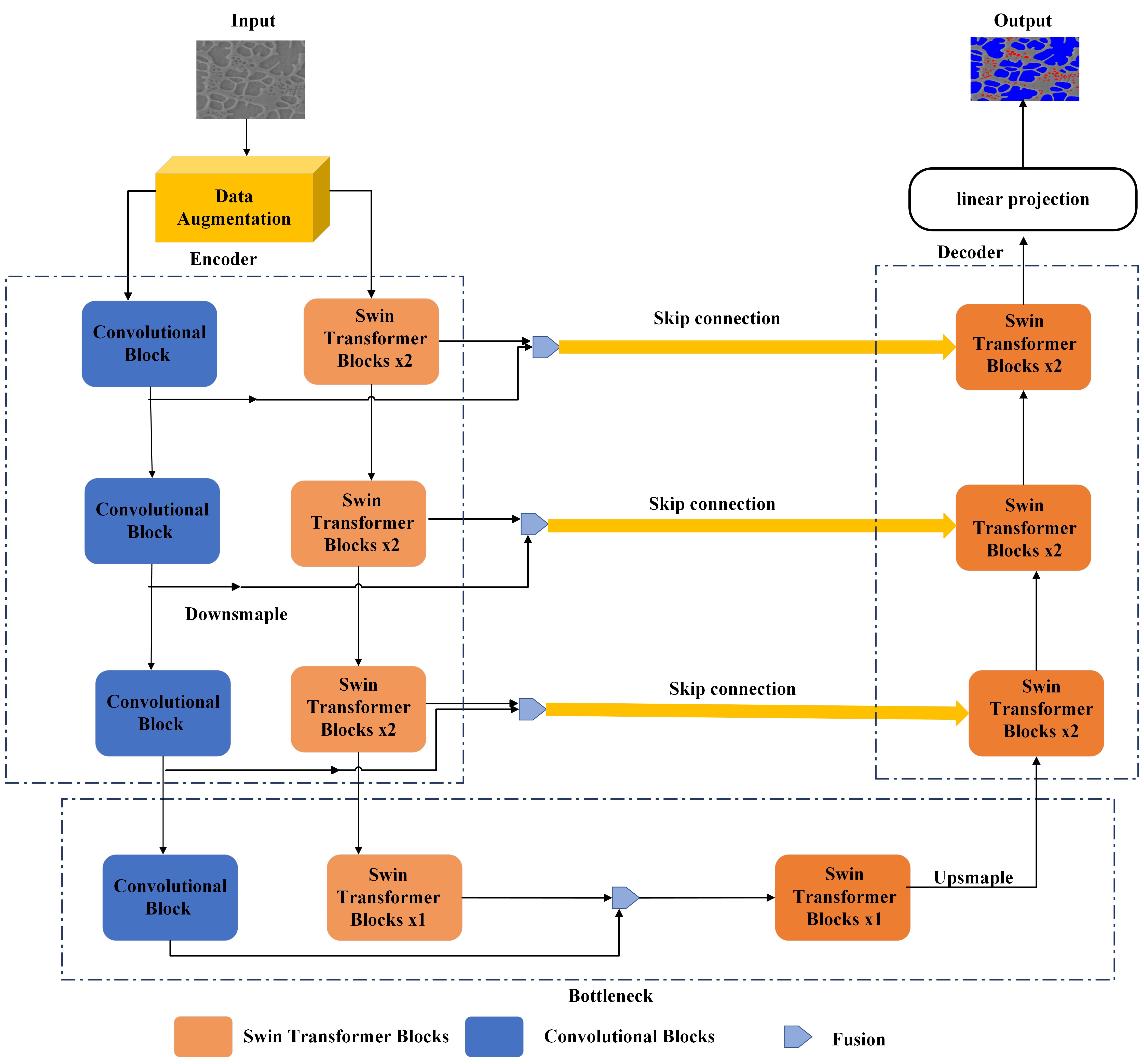
Figure 3: : Overview of the proposed CS-UNet architecture consist of encoder, bottleneck, and decoder, where the encoder part includes CNN and Swin-T.

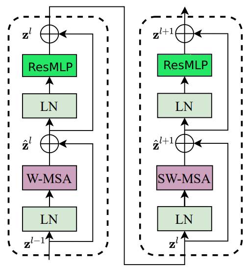
Figure 4: ResMLP used to improve Swin Transformer block [37].

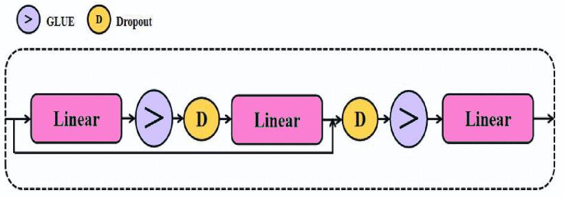
Figure 5: ResMLP module block [37].

The encoder combines a CNN encoder and a Swin-T encoder, where CNN is used to extract low-level features and Swin-T is used to extract global contextual features. The Swin-T encoder operates on the input image divided into non-overlapping patches, applying self-attention mechanisms to capture global dependencies. The encoder captures long-range dependencies and contextual information from the entire image at different scales. Inspired by the TFCN (Transformers for Fully Convolutional dense Net) [38] and Lightweight Swin-Unet [37], the Multi-Layer Perceptron (MLP) in two successive Swin-T blocks was replaced by Residual Multi-Layer Perceptron (ResMLP). As illustrated in Figure 4, ResMLP is used to reduce feature loss in the transmission process and to increase the contextual information extracted by the encoder. ResMLP is illustrated in Figure 5, which consists of two GELU [39] nonlinear layers, three Linear layers, and two dropout layers. The CNN encoder processes the input image in a series of convolution layers, gradually reducing the spatial dimensions while extracting hierarchical features. Along the way, the encoder captures low-level features in early layers and higher-level semantic features in deeper layers.

To fuse the information from both encoders, the skip connections concatenate the feature maps from the CNN encoder and the Swin-T encoder with the corresponding decoder layers. To ensure compatibility between the feature dimensions of the CNN and the Swin-T encoders, it is necessary to normalize the dimensions before fusing them. This is achieved by passing the features obtained from the CNN block through a linear embedding layer, which flattens and reshapes the feature map from the shape of $(B,C,H,W)$ to $(B,C,H\times W)$, where $B$, $C$, $H$, $W$ are the batch size, the number of channels, the height, and the width of the feature map, respectively. The flattened feature map is transposed to swap the last two dimensions resulting in the shape of $(B,H\times W,C)$ and is then fused with extracted features from the Swin-T encoder. By fusing the information from different encoder pathways, the skip connections enable the decoder to benefit from both the local spatial details captured by the CNN encoder and the global context captured by the Swin-T encoder.

The decoder is similar to that of Swin-Unet[19], which employs the patch-expanding layer to up-sample the extracted deep features by reshaping the feature maps of adjacent dimensions to form a higher-resolution feature map, which effectively achieves a $2\times$ up-sampling. Additionally, it reduces the feature dimension to half of the original dimension. This allows the decoder to reconstruct the output with increased spatial resolution while reducing the feature dimension for efficient processing. The final patch-expanding layer further performs a $4\times$ up-sampling to restore the resolution of the feature maps to match the input resolution $(W\times H)$. Finally, a linear projection layer is applied to these up-sampled features to generate pixel-level segmentation predictions.

Different CNN families can be used in the encoder part such as EfficientNet, ResNet, MobileNet, DenseNet, VGG, and Inception. We initialize CNN weights using MicroNet and the transformer weights using MicroLite.

4 Results

The pre-trained Swin-T models were used to classify microscopy images among 74 different classes. Swin-T models were either pre-trained on ImageNet (specifically the imageNet1K dataset) and fine-tuned on MicroLite or trained with MicroLite with randomized parameters. The training stops when the validation accuracy does not improve after 5 epochs. The model accuracy is evaluated using the top-1 and top-5 accuracy. The top-1 accuracy measures the percentage of test samples for which the correct label is predicted while the top-5 accuracy measures the percentage of correct labeling in the top five predictions.

As shown in Table I, the Swin-T models, when trained from scratch, take longer to converge. Specifically, the original Swin-T model takes 23 epochs, while the intermediate version takes 19 epochs. In contrast, the Swin-T models pre-trained on the ImageNet and then fine-tuned on the MicroLite converge faster. The original Swin-T model takes only 13 epochs, while the intermediate version takes 12 epochs. On average, the models initialized with ImageNet weights converged about 40.16% faster than those with the random initialization. Original Swin-T fine-tuned on MicroLite after pre-training with ImageNet achieved the top-1 accuracy of 84.63%. Overall, the Swin-T models pre-trained on ImageNet and fine-tuned on MicroLite have higher accuracy and faster convergence.

TABLE I: Classification accuracy of pre-trained models, where the “ImageNet → MicroLite” indicate that the models were pre-trained on ImageNet and then fine-tuned on MicroLite.

Swin-T architecture	Pre-training method	top-1 accuracy	top-5 accuracy	# of epochs to converge
Original	MicroLite	84.23	95.91	23
	ImageNet → MicroLite	84.63	96.353	13
Intermediate	MicroLite	84.0	96.91	19
	ImageNet → MicroLite	84.45	97.83	12

4.1 Microstructural Image Segmentation

To evaluate how well the Swin-T models can extract feature representations, the pre-trained models were used to initialize the models for segmentation tasks. To allow comparison to the NASA study [1], we used the same 7 microscopy datasets derived from two materials: nickel-based super-alloys (Super) and Environmental Barrier Coatings (EBC). EBC datasets have two classes: the oxide layer and the background (non-oxide) layer, Super datasets have 3 classes: matrix, secondary, and tertiary. The number of images in each dataset split is shown in Table II. Super-1 and EBC-1 contain the full dataset labeled for their respective materials. Super-2 and EBC-2 have only 4 images in the training set to evaluate the performance of the models in a few shots. Super-3 and EBC-3 have only 1 image in the training set to evaluate performance during the one-shot learning. Super-4 have test images taken under different imaging and sample conditions. All segmentation models in this study were trained using PyTorch [40].

TABLE II: Number of Microscopy images in the training, validation, and test set for each experimental dataset

Experiment	# of training images	# of validation images	# of test images
Super-1	10	4	4
Super-2	4	4	4
Super-3	1	4	4
Super-4	4	4	5
EBC-1	18	3	3
EBC-2	4	3	3
EBC-3	1	3	3

EBC and Super datasets were augmented in ways similar to the NASA study [1], which includes random cropping to $512\times 512$ pixels, random changes to contrast, brightness, and gamma, and added blurring or sharpening. EBC dataset was horizontally flipped and Super dataset was randomly flipped vertically and horizontally and rotated. The training used an Adam optimizer with an initial learning rate of $2\times 10^{-4}$ until the validation accuracy showed no improvement for 30 epochs. Afterwards, the training continued with a learning rate of $10^{-5}$ until early stopping was triggered after an additional 30 epochs without any validation improvement. Since the datasets are imbalanced, the loss function was set by the weighted sum of Balanced Cross Entropy (BCE) and dice loss with a 70% weighting towards BCE [1].

TABLE III: The combinations of encoders in CS-UNet, where the second column shows the pre-training models for the Swin-T encoders and the third column shows the pre-training models for the CNN encoders. The last column shows the models for both types of encoders, where ‘Microscopy’ is either MicroNet or MicroLite.

Swin-T architecture	Swin-T pre-training model	CNN pre-training model	CS-UNet pre-training model
Original	ImageNet	ImageNet	ImageNet
Original	MicroLite	MicroNet	Microscopy
Original	ImageNet → MicroLite	ImageNet → MicroNet	ImageNet → Microscopy
Intermediate	MicroLite	MicroNet	Microscopy
Intermediate	ImageNet → MicroLite	ImageNet → MicroNet	ImageNet → Microscopy

The CS-UNet architecture is a flexible model that can be trained with different CNN families and initialized with different pre-trained models. Table III shows the various combinations of pre-trained weights that were used to train the CS-UNet model. The second column shows the pre-trained weights that initialize the Swin-T encoder and the third column shows the pre-trained weights that initialize the CNN encoder. In the last column, we use the term Microscopy to refer to the case where CNN encoders are trained with MicroNet and Transformer encoders are trained with MicroLite. Other combinations of pre-trained weights can also be used to train the CS-Unet model. For example, the Swin-T encoder could be initialized with the MicroLite weights and the CNN encoder could be initialized with the ImageNet→MicroNet weights. The flexibility of the CS-UNet architecture allows researchers to experiment with different combinations of pre-trained weights to find the best combination for their specific task.

TABLE IV: Comparison of the top performance (IoU) of UNet++/UNet pre-trained on MicroNet [1], Transformer segmentation models pre-trained on MicroLite, and CS-UNet pre-trained on MicroNet and MicroLite.

Dataset	UNet++/UNet + MicroNet	Transformer + MicroLite	CS-UNet + MicroNet + MicroLite
Super-1	96.4%	95.72%	96.43%
Super-2	94.2%	95.16%	96.06%
Super-3	93.0%	92.23%	93.5%
Super-4	78.5%	78.91%	82.13%
EBC-1	97.6%	96.59%	97.66%
EBC-2	93.3%	91.11%	92.82%
EBC-3	65.9%	82.13%	70.46%

Table IV compares the top performance of UNet++/UNet pre-trained on MicroNet (the numbers were reported in Figure 3–5 of [1]), Transformer models (including Swin-UNet, TransDeepLabV3+, and HiFormer) pre-trained on MicroLite, and CS-UNet pre-trained on MicroNet and MicroLite. The highest accuracy for each experiment is shown in bold font. CS-UNet has the best performance in most experiments except EBC-2 and EBC-3. For experiments with ample training data such as Super-1 and EBC-1, the difference between UNet++/UNet, Transformer, and CS-UNet is small. For few-shot learning experiments such as Super-2 and EBC-2, the accuracy gain of CS-UNet is modest. For one-shot learning experiments, the result is mixed, where CS-UNet has modest improvement in Super-3 while significant gain in EBC-3. For out of context learning, CS-UNet shows significant improvement over UNet or Transformer.

Overall, the results of the table suggest that CS-UNet is a promising approach for image segmentation tasks. CS-UNet is similar or significantly better than UNet++/UNet in all experiments and it is better than Transformers for most experiments. Note that MicroLite is about half the size of MicroNet. Despite this, Transformer + MicroLite has comparable or better performance than that of UNet++/UNet + MicroNet. Appendix A shows the configurations of the best performing Transformer models shown in Table IV. The configurations of the best performing CS-UNet models are shown in the next section, where we compare the performance of CS-UNet when it is pre-trained on microscopy images and on ImageNet.

4.2 Nickel-based Super-alloy (Super) Segmentation

Figure 6 and Figure 7 compare the best performance of CS-UNet on Super datasets when it is pre-trained on the microscopy images and ImageNet. The IoU scores for Super-1 and Super-2 are similar for both pre-training models while the IoU score for Super-3 is significantly higher for microscopy model at 93.5% in comparison to the 87.01% of the ImageNet model. This result differs from that of the NASA paper, where the performance of Super-2 was also increased. It appears that with the enhanced ability of CS-UNet, the benefit of in-domain dataset is more significant in one-shot learning than few-shot learning. The ImageNet model failed to identify many of the tertiary precipitates in the dark contrast images, as indicated by the orange triangles. The ImageNet model also over-segmented and combined some of the secondary precipitates, as indicated by the green arrows.

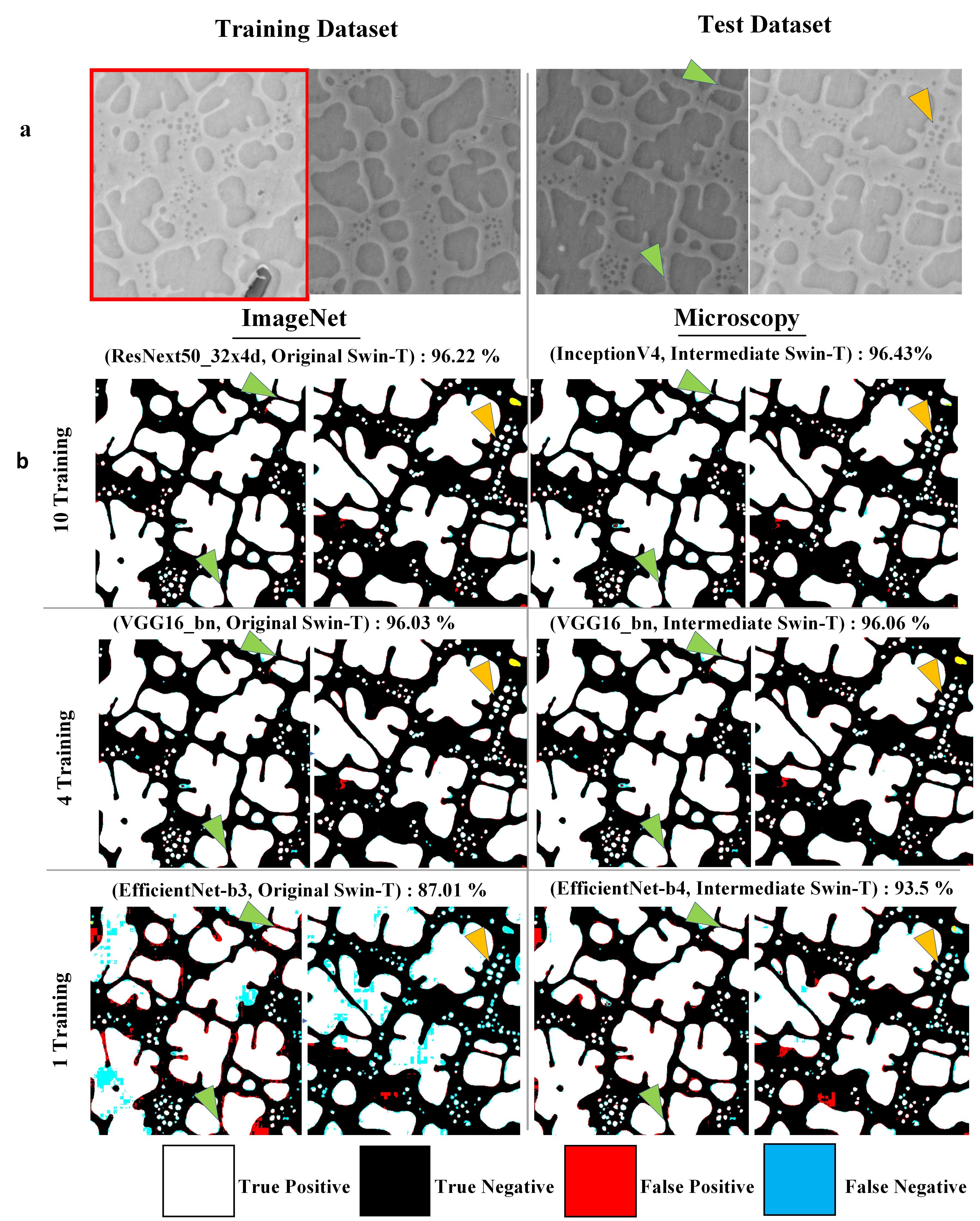
Figure 6: (a) are examples of the training and test images of the Super datasets [1], where the training image of Super-3 is outlined in red. (b) are the best segmentation masks of the test images when CS-UNet is trained with Super-1, Super-2, and Super-3 dataset, where the left is pre-trained with ImageNet and the right is pre-trained with microscopy images. The CNN/Transformer encoders and the IoU score of the best model are above the segmentation mask of each experiment. The green triangle points to the area where the ImageNet (but not the microscopy) model incorrectly segmented the secondary precipitates. The yellow triangle points to the area where the ImageNet (but not the microscopy) model incorrectly segmented the tertiary precipitates.

For Super-4, which contains images with different imaging conditions, microscopy model improves the performance of ImageNet model from 78.89% to 82.13%, which is consistent with the findings of the NASA paper. As shown in Figure 7, the test images of Super-4 comes from a different image distribution than the training images (Figure 6). The first row shows a micrograph that comes from a different alloy. Rows (2 and 3) show micrographs with different etching conditions, and the last row shows micrograph with poor imaging [1]. The microscopy model is more accurate and less over-segmented for separating the secondary precipitates than the ImageNet model, where the differences are marked with green arrow. The microscopy model performs better for the secondary and the tertiary precipitate of the segmented images.

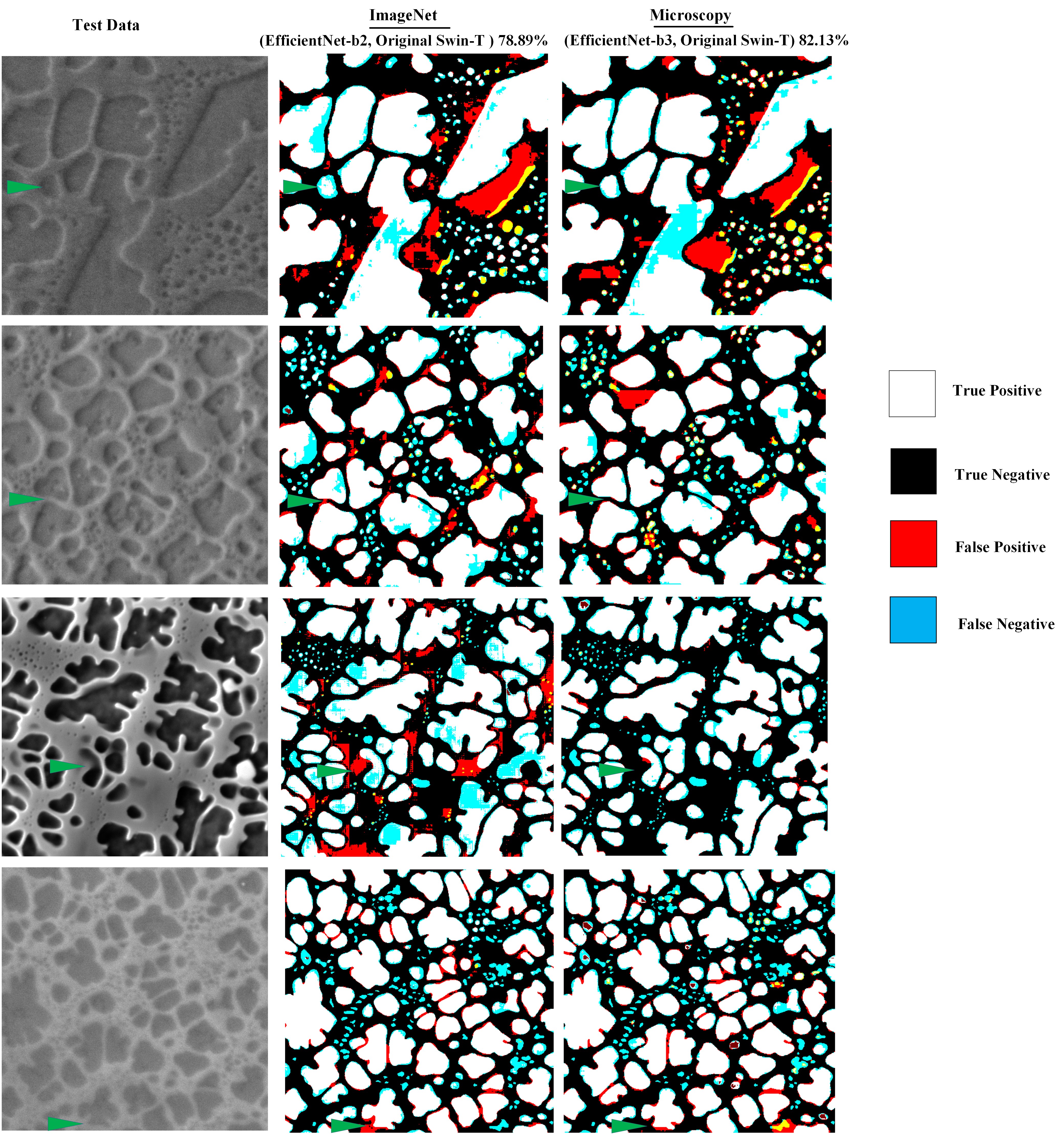
Figure 7: The test images of Super-4 have different imaging conditions than those of the training images. The left column shows the test images of Super-4 [1]. The accuracy mask colors are the same as those in Figure 6. The middle column shows the IoU accuracy masks for the best ImageNet model. The right column shows the same for the best microscopy model. Each row shows the test image and accuracy masks of the same image. The green arrow shows an example where the model was over-segmented and where the microscopy model accurately segmented the secondary precipitate. The yellow color indicates incorrect identification of a tertiary precipitate as a secondary precipitate. The maroon color indicates where the model improperly identified a secondary precipitate as a tertiary precipitate. The cyan color indicates where the model over-segmented the secondary precipitates.

4.3 Environmental Barrier Coating (EBC) Segmentation

As shown in Figure 8, the results of EBC datasets are consistent with the findings of the NASA paper, where the IoU scores of EBC-1 and EBC-2 are similar for both the microscopy and the ImageNet models. The segmentation outputs of EBC-1 and EBC-2 for both models are able to distinguish between the substrate and the thermally grown oxide layer and they are useful for oxide thickness measurements after simple morphological operations.

EBC-3 has one training image (outlined in red in Figure 8). The IoU score of the best microscopy model is 70.46% much higher than the IoU of 61.74% of the best ImageNet model. This also confirms the result of the NASA paper though our improvement is much larger. The ImageNet model is not able to distinguish between the substrate and the thermally grown oxide layer, which made it impossible to accurately measure oxide thickness.

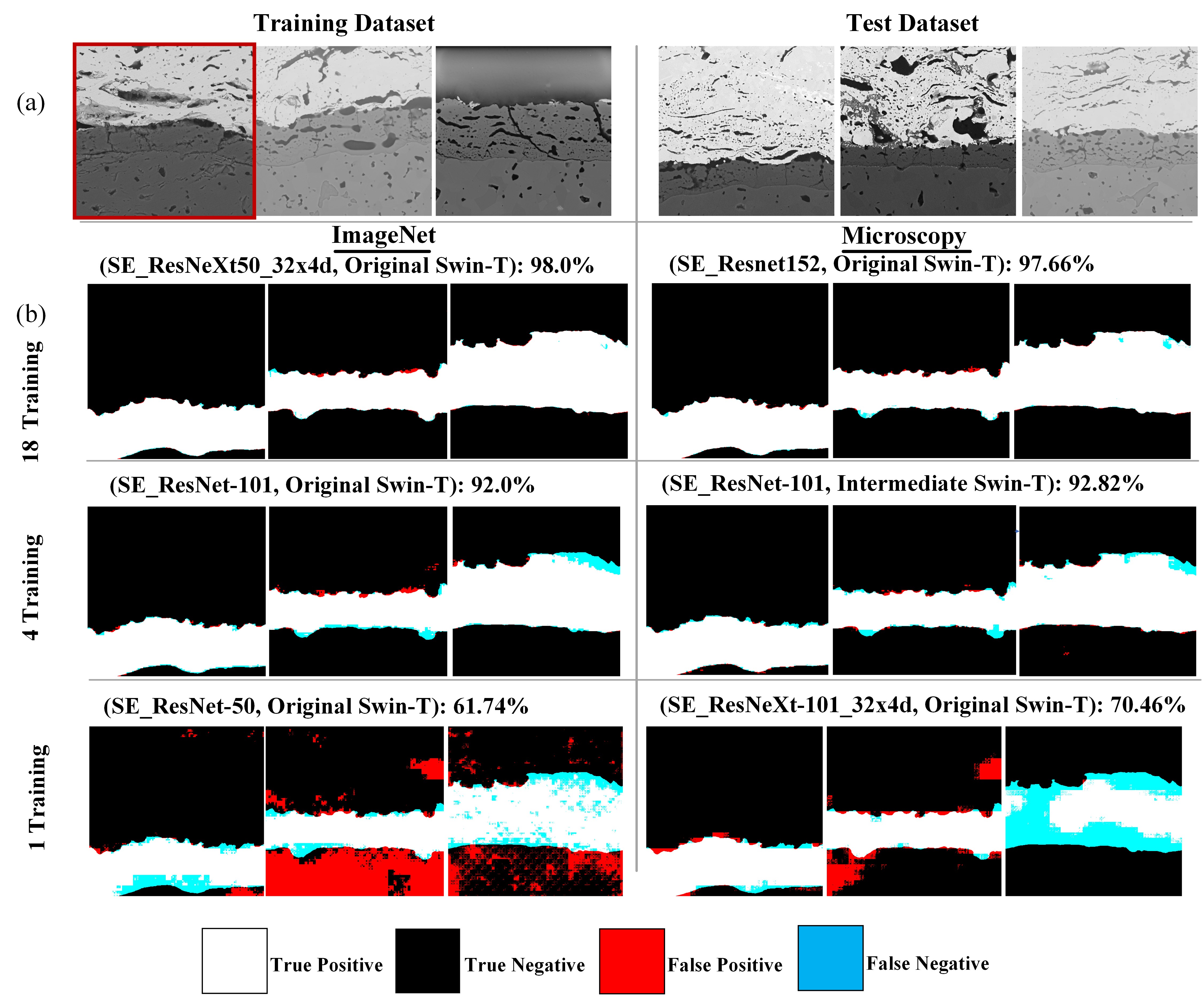
Figure 8: (a) shows examples of the train and test images in the EBC datasets, where the left column represents the training set and the right column represents the test set. The single training image for EBC-3 is outlined in red. (b) shows the segmentation results for the top ImageNet and microscopy models for each EBC dataset. The CNN/Transformer encoders and the IoU score of the best model is above the segmentation mask of each experiment.

5 Discussion

We have shown that CNN and Transformer encoders in CS-UNet provide better segmentation performance than CNN encoders alone in UNet. We have also shown that pre-training on microscopy images provide better performance for CS-UNet than pre-training on ImageNet, though the degree of improvement differs from that observed on UNet. Nevertheless, these comparisons are based on best performing models. Depending on the choice of CNN encoders, Transformer architectures, and pre-training models, the segmentation performance can vary significantly.

In this section, we compare the impact of pre-training on the average performance of CNN-based, Transformer-based, and hybrid segmentation algorithms. After that, we compare the average performance of the three types of segmentation algorithms. Our results indicate that pre-training on microscopy images generally has positive impacts to the performance. Our hybrid algorithm CS-UNet outperforms UNet in all experiments while it has similar or better performance than Transformer-based algorithms.

5.1 CNN-based Image Segmentation

TABLE V: The average performance of UNet when it is initialized with different pre-training weights. Each entry shows the mean and standard deviation of IoU value for a pre-training model. The highest score for each test is in bold.

Dataset	ImageNet	MicroNet	ImageNet→MicroNet
Super-1	96.09%±0.20%	95.99%±0.16%	95.92%±0.19%
Super-2	95.08%±1.27%	95.28%±0.26%	95.38±1.03%
Super-3	63.30%±4.55%	74.61%±17.21%	78.69±11.24%
Super-4	71.46%±6.88%	75.1%±9.0%	77.78%±0.17
EBC-1	95.18%±0.82%	94.65%±1.44%	95.69%±1.03%
EBC-2	80.74%±10.76%	87.06%±1.55%	86.0%±5.17%
EBC-3	39.36%±7.81%	41.95%±4.89%	46.44%±4.35%

We first examine the performance of UNet [15] with 3 types of encoder pre-training. We include this result since the configurations of CS-UNet only used 19 of the 35 CNN encoders in the NASA paper [1]. As shown in Appendix B, the 19 encoders have top-5 accuracy in at least one of the segmentation tasks. This selection reduces the number of experiments needed for a fair comparison,

The average performance of UNet when it is pre-trained with ImageNet or MicroNet is in Table V, which indicates that ImageNet→MicroNet model (i.e. CNN encoders initialized with ImageNet model and fine-tuned with MicroNet) achieves the best outcome in majority of the cases. The configurations of the top-performing CNN encoders are shown in Appendix C, which also indicates that pre-training on MicroNet provides better outcome in most of the cases.

Unsurprisingly, our results are largely consistent with that of the NASA paper [1], since we used their pre-training models on MicroNet. Specifically, pre-training with MicroNet improves the performance of one-shot and out-of-distribution learning. Since we picked CNN encoders that have top-5 performance in at least one experiment, the IoU scores are higher than the average scores shown in the NASA paper. In fact, the performances on Super-2 (few-shot learning) are basically the same with different pre-training models.

5.2 Transformer-based Image Segmentation

TABLE VI: Average performance of Transformer-based segmentation algorithms when initialized with different pre-training weights. Each entry shows the mean and standard deviation of IoU value for a pre-training model. The highest score for each dataset is in bold.

Swin-T arch.	Original			Intermediate
Dataset	ImageNet	MicroLite	ImageNet→MicroLite	MicroLite	ImageNet→MicroLite
Super-1	94.94%±0.31%	95.0%±0.43%	94.89%±0.45%	94.72%±0.97%	94.41%±0.51%
Super-2	93.26%±0.76%	93.83%±0.62%	93.55%±0.30%	94.03%±0.83%	93.43%±0.97%
Super-3	76.24%±7.06%	79.53%±13.69%	70.65%±10.74%	78.74%±17.08%	69.31%±6.44%
Super-4	73.04%±1.64%	73.18%±1.81%	72.89%±2.93%	72.10%±2.39%	71.23%±2.32%
ECB-1	91.73%±3.40%	94.67%±1.59%	91.44%±2.87%	94.95%±1.41%	90.56%±3.01%
ECB-2	82.47%±5.90%	86.02%±4.98%	83.20%±3.34%	86.67%±2.61%	83.07%±4.22%
ECB-3	52.21%±6.76%	65.90%±13.12%	55.15%±10.42%	56.91%±5.24%	49.03%±4.67%

Next, we show in Table VI the average performance of Transformer-based segmentation algorithms (Swin-UNet, HiFormer, and TransDeepLabv3+) using different configurations of pre-training and Swin-T architectures. We compared the algorithms by using the original or the intermediate Swin-T architecture and by initializing their weights with ImageNet or microscopy pre-training models. Our results indicate that the algorithms perform well with the MicroLite pre-training model and that the original Swin-T architecture is slightly better with 1-shot learning and out-of-distribution learning. Overall, pre-training with microscopy images provided better results for Transformer-based segmentation algorithms than pre-training on natural images.

5.3 Hybrid Image Segmentation

TABLE VII: Average performance of CS-UNet when initialized with different pre-training weights for each experiment. Each entry in the table shows the mean value and standard deviation of the evaluation IoU metric for a particular pre-training model. The highest accuracy score for each dataset is shown in bold.

Swin-T arch.	Original			Intermediate
Dataset	ImageNet	Microscopy	ImageNet → Microscopy	Microscopy	ImageNet → Microscopy
Super-1	96.11%±0.11%	96.19%±0.13%	96.16%±0.14%	96.22%±0.15%	96.02%±0.34%
Super-2	95.63%±0.23%	95.63%±0.44%	95.78%±0.14%	95.67%±0.46%	95.86%±0.11%
Super-3	78.64%±9.3%	76.59%±15.78%	78.01%±13.32%	78.18%±12.13%	80.68%±12.60%
Super-4	73.74%±3.74%	77.25%±3.31%	72.87%±6.26%	76.65%±2.53%	75.07%±1.10%
ECB-1	97.09%±0.86%	95.48%±1.04%	96.4%±0.79%	94.72%±1.37%	96.21%±0.78%
ECB-2	83.57%±7.71%	86.12%±1.76%	88.58%±1.46%	86.41%±1.65%	88.08%±2.98%
ECB-3	45.88%±10.12%	44.7%±8.57%	46.08%±13.92%	46.35%±9.91%	45.16%±10.58%
mean IoU	81.5	81.71	81.98	82.03	82.44

We also compare the performance of our hybrid segmentation algorithm CS-UNet in Table VII when it uses the original or the intermediate Swin-T architecture and when it is initialized with weights from ImageNet or microscopy models. Since CS-UNet uses both CNN and Transformer encoders, the results are mixed where pre-training with microscopy images does not provide better performance in all cases. The weaker performance of CNN encoders reduced the advantage of Transformer encoders when they are pre-trained on microscopy images. When we consider the mean IoU scores across all experiments, however, pre-training with microscopy images still offers some benefits.

5.4 Comparison of Segmentation Networks

TABLE VIII: The average performance of CNN, Transformer, and CS-UNet on all datasets. Each entry in the table shows the mean value and standard deviation of the IoU evaluation metric for a particular method.

Dataset	UNet [15]	CS-UNet	Swin-Unet [19]	TransDeepLabV3+ [23]	HiFormer [22]
Super-1	95.98% $\pm$ 0.20%	96.14% $\pm$ 0.21%	95.30%$\pm 0.34$ %	94.91% $\pm$ 0.47%	94.30% $\pm$ 0.58%
Super-2	95.24% $\pm$ 0.96%	95.70% $\pm$ 0.33%	93.39% $\pm$ 1.1%	94.1% $\pm$ 0.61%	93.11% $\pm$ 0.5%
Super-3	72.20% $\pm$ 13.79%	77.99% $\pm$ 12.90%	83.0% $\pm$ 6.14%	81.99% $\pm$ 8.29%	64.19% $\pm$ 8.14%
Super-4	74.57% $\pm$ 7.23%	75.08% $\pm$ 4.15%	77.16% $\pm$ 0.97%	70.95% $\pm$ 1.86%	72.61% $\pm$ 1.67%
EBC-1	95.17% $\pm$ 1.21%	95.98% $\pm$ 1.28	93.49$\pm$ 2.66%	91.59% $\pm$ 4.13%	93.96% $\pm$ 1.1%
EBC-2	84.60% $\pm$ 7.48%	86.73%$\pm$ 4.03%	83.13% $\pm$ 3.1%	83.1% $\pm$ 5.68%	86.67% $\pm$ 1.44%
EBC-3	42.58% $\pm$ 6.57%	45.69% $\pm$ 10.78%	58.62% $\pm$ 20.37%	58.7% $\pm$ 9.70%	52.84% $\pm$ 5.41%

Lastly, we compare the performance of the 3 types of segmentation algorithms (UNet, CS-UNet, Swin-Unet, HiFormer, and TransDeepLabv3+) averaged over different pre-training models and Swin-T architectures in Table VIII. The results show that CS-UNet is better than UNet on average across all experiments. While Transformer-based segmentation algorithms may be superior in 1-shot learning or out-of-distribution learning, their performance is not always consistently better than UNet. Therefore, our hybrid algorithm CS-UNet appears to be the more robust solution regardless of the pre-training models.

6 Conclusion

In this paper, we demonstrated that training CNN and Transformer encoders on an in-domain dataset can lead to better feature representations for image segmentation. We introduced CS-UNet – a hybrid network that combines CNN and Swin Transformer encoders for image segmentation. The encoders of CS-UNet extract low-level and high-level features from input images while the decoder part employs Swin Transformers for image segmentation. We show that CS-UNet generally outperforms UNet in our experiments and it has competitive performance compared to Transformer-based algorithms. The hybrid nature of CS-UNet enables effective segmentation of images with long-range dependencies and high spatial resolution.

Our pre-training dataset is limited in size. A larger dataset will produce better feature representation of microstructures through pre-training, which improves the accuracy of downstream analysis tasks. While CS-UNet can preserve spatial information and process long-range dependencies, it is computationally intensive compared to CNN and Transformer-based algorithms. As future work, we will explore the training of other Transformer architectures, such as Focal Transformer and FocalNet, on large microscopy datasets. These architectures may offer further advancements in image segmentation, expanding the range of available options and potential improvements in materials analysis tasks.

Appendix A Transformer Performance

Table IX shows the best-performing configurations of Transformer-based segmentation algorithms. Note that for pre-training with MicroLite, direct training with MicroLite resulted in the best performance in all cases except Super-4, where ImageNet→MicroLite has the best performance.

TABLE IX: The best performing configurations of Transformer-based segmentation algorithms.

Dataset	ImageNet		MicroLite
	best performing configuration	IoU	best performing configuration	IoU
Super-1	TransDeepLabV3+ / Orginal Swin-T	95.25%	Swin-Unet / Intermediate Swin-T	95.72%
Super-2	Swin-Unet / Orginal Swin-T	94.37%	TransDeepLabV3+ / Intermediate Swin-T	95.16%
Super-3	Swin-Unet / Orginal Swin-T	89.78%	TransDeepLabV3+ / Intermediate Swin-T	92.23%
Super-4	Swin-Unet / Orginal Swin-T	76.42%	Swin-Unet / Orginal Swin-T	78.91%
EBC-1	Swin-Unet / Orginal Swin-T	96.11%	TransDeepLabV3+ / Intermediate Swin-T	96.59%
EBC-2	HiFormer / Orginal Swin-T	84.21%	TransDeepLabV3+ / Orginal Swin-T	91.11%
EBC-3	TransDeepLabV3+ / Orginal Swin-T	65.77%	Swin-Unet / Orginal Swin-T	82.13%

Appendix B Selected CNN Encoders

Table X shows the 19 CNN encoders that were chosen to evaluate the performance of CS-UNet and UNet.

TABLE X: Each encoder has at least 1 top-5 average IoU score for Super/EBC datasets (based on Figure 4 of [1]).

CNN Encoder	Super-1	Super-2	Super-3	Super-4	EBC-1	EBC-2	EBC-3
SE_ResNet-50 [41]							✓
SE_ResNeXt-50_32x4d [42]	✓	✓			✓	✓	✓
SE_ResNeXt-101_32x4d [42]	✓	✓					✓
SE_ResNet-152 [41]	✓				✓
SE_ResNet-101 [41]					✓	✓	✓
SENet-154 [41]		✓	✓		✓
ResNeXt-101_32x8d [42]	✓
Inception-V4 [43]		✓	✓		✓
Inception-ResNet-V2 [43]			✓
DenseNet201 [44]						✓
DenseNet161 [44]						✓
VGG-16_bn [45]	✓		✓			✓
VGG-13_bn [45]			✓
MobileNet-V2 [46]							✓
EfficientNet-b1 [47]				✓
EfficientNet-b2 [47]				✓
EfficientNet-b3 [47]				✓
EfficientNet-b4 [47]				✓
EfficientNet-b5 [47]		✓		✓

Appendix C UNet Performance

Table XI shows the CNN encoders that produced the best performance of UNet for each dataset when pre-trained on ImageNet or MicroNet. EfficientNet and Se_ResNet families have better performance than the older encoder families such as VGG.

TABLE XI: The best performing CNN encoders of UNet that are pre-trained on ImageNet and MicroNet.

Dataset	ImageNet		MicroNet
	best performing CNN encoder	IoU	best performing CNN encoder	IoU
Super-1	SE_ResNeXt-50_32x4	96.2%	SE_ResNeXt-101_32x4d	95.95%
Super-2	EfficientNet-b5	95.45%	SENet-154	95.50%
Super-3	EfficientNet-b3	70.74%	EfficientNet-b3	92.5%
Super-4	EfficientNet-b2	77.34%	EfficientNet-b1	78.95%
EBC-1	SENet-154	96.23%	SENet-154	96.67%
EBC-2	DenseNet201	91.36%	InceptionResnetV2	90.97%
EBC-3	EfficientNet-b3	44.4%	EfficientNet-b3	52.84%

DATA AVAILABILITY

The pre-trained Swin-T models of our experiments are available at our GitHub repository:

https://github.com/Kalrfou/SwinT-pretrained-microscopy-models.

This work also used the pre-trained CNN models from

https://github.com/nasa/pretrained-microscopy-models.

AUTHOR CONTRIBUTIONS

Alrfou developed the CS-UNet method, conceived and designed the study, developed the software, evaluated results, provided datasets, and contributed to the formal analysis and writing of the original draft. Zhao and Kordijazi evaluated the results, contributed to the formal analysis and writing of the original draft, and proofread and reviewed the final manuscript.

References

- [1] J. Stuckner, B. Harder, and T. M. Smith, “Microstructure segmentation with deep learning encoders pre-trained on a large microscopy dataset,” npj Computational Materials, vol. 8, no. 1, p. 200, 2022.
- [2] M. Ge, F. Su, Z. Zhao, and D. Su, “Deep learning analysis on microscopic imaging in materials science,” Materials Today Nano, vol. 11, p. 100087, 2020.
- [3] K. Choudhary, B. DeCost, C. Chen, A. Jain, F. Tavazza, R. Cohn, C. W. Park, A. Choudhary, A. Agrawal, S. J. Billinge et al., “Recent advances and applications of deep learning methods in materials science,” npj Computational Materials, vol. 8, no. 1, p. 59, 2022.
- [4] A. Dosovitskiy, L. Beyer, A. Kolesnikov, D. Weissenborn, X. Zhai, T. Unterthiner, M. Dehghani, M. Minderer, G. Heigold, S. Gelly et al., “An image is worth 16x16 words: Transformers for image recognition at scale,” arXiv preprint arXiv:2010.11929, 2020.
- [5] K. Alrfou, A. Kordijazi, and T. Zhao, “Computer vision methods for the microstructural analysis of materials: The state-of-the-art and future perspectives,” arXiv preprint arXiv:2208.04149, 2022.
- [6] G. Jacquemet, “Deep learning to analyse microscopy images,” The Biochemist, vol. 43, no. 5, pp. 60–64, 2021.
- [7] Z. Liu, Y. Lin, Y. Cao, H. Hu, Y. Wei, Z. Zhang, S. Lin, and B. Guo, “Swin transformer: Hierarchical vision transformer using shifted windows,” in Proceedings of the IEEE/CVF international conference on computer vision, 2021, pp. 10 012–10 022.
- [8] A. Vaswani, N. Shazeer, N. Parmar, J. Uszkoreit, L. Jones, A. N. Gomez, Ł. Kaiser, and I. Polosukhin, “Attention is all you need,” Advances in neural information processing systems, vol. 30, 2017.
- [9] L. Ye, M. Rochan, Z. Liu, and Y. Wang, “Cross-modal self-attention network for referring image segmentation,” in Proceedings of the IEEE/CVF conference on computer vision and pattern recognition, 2019, pp. 10 502–10 511.
- [10] J. Dai, “Deformable detr: Deformable transformers for end-to-end object detection.”
- [11] N. Carion, F. Massa, G. Synnaeve, N. Usunier, A. Kirillov, and S. Zagoruyko, “End-to-end object detection with transformers,” in Computer Vision–ECCV 2020: 16th European Conference, Glasgow, UK, August 23–28, 2020, Proceedings, Part I 16. Springer, 2020, pp. 213–229.
- [12] H. Zhang, I. Goodfellow, D. Metaxas, and A. Odena, “Self-attention generative adversarial networks,” in International conference on machine learning. PMLR, 2019, pp. 7354–7363.
- [13] C. Sun, A. Shrivastava, S. Singh, and A. Gupta, “Revisiting unreasonable effectiveness of data in deep learning era,” in Proceedings of the IEEE international conference on computer vision, 2017, pp. 843–852.
- [14] Z. Liu, H. Hu, Y. Lin, Z. Yao, Z. Xie, Y. Wei, J. Ning, Y. Cao, Z. Zhang, L. Dong et al., “Swin transformer v2: Scaling up capacity and resolution,” in Proceedings of the IEEE/CVF conference on computer vision and pattern recognition, 2022, pp. 12 009–12 019.
- [15] O. Ronneberger, P. Fischer, and T. Brox, “U-net: Convolutional networks for biomedical image segmentation,” in Medical Image Computing and Computer-Assisted Intervention–MICCAI 2015: 18th International Conference, Munich, Germany, October 5-9, 2015, Proceedings, Part III 18. Springer, 2015, pp. 234–241.
- [16] K. Alrfou, A. Kordijazi, P. Rohatgi, and T. Zhao, “Synergy of unsupervised and supervised machine learning methods for the segmentation of the graphite particles in the microstructure of ductile iron,” Materials Today Communications, vol. 30, p. 103174, 2022.
- [17] E. Xie, W. Wang, Z. Yu, A. Anandkumar, J. M. Alvarez, and P. Luo, “Segformer: Simple and efficient design for semantic segmentation with transformers,” Advances in Neural Information Processing Systems, vol. 34, pp. 12 077–12 090, 2021.
- [18] J. Chen, Y. Lu, Q. Yu, X. Luo, E. Adeli, Y. Wang, L. Lu, A. L. Yuille, and Y. Zhou, “Transunet: Transformers make strong encoders for medical image segmentation,” arXiv preprint arXiv:2102.04306, 2021.
- [19] H. Cao, Y. Wang, J. Chen, D. Jiang, X. Zhang, Q. Tian, and M. Wang, “Swin-unet: Unet-like pure transformer for medical image segmentation,” in European Conference on Computer Vision. Springer, 2022, pp. 205–218.
- [20] A. Hatamizadeh, Y. Tang, V. Nath, D. Yang, A. Myronenko, B. Landman, H. R. Roth, and D. Xu, “Unetr: Transformers for 3d medical image segmentation,” in Proceedings of the IEEE/CVF winter conference on applications of computer vision, 2022, pp. 574–584.
- [21] A. Hatamizadeh, V. Nath, Y. Tang, D. Yang, H. R. Roth, and D. Xu, “Swin unetr: Swin transformers for semantic segmentation of brain tumors in mri images,” in Brainlesion: Glioma, Multiple Sclerosis, Stroke and Traumatic Brain Injuries: 7th International Workshop, BrainLes 2021, Held in Conjunction with MICCAI 2021, Virtual Event, September 27, 2021, Revised Selected Papers, Part I. Springer, 2022, pp. 272–284.
- [22] M. Heidari, A. Kazerouni, M. Soltany, R. Azad, E. K. Aghdam, J. Cohen-Adad, and D. Merhof, “Hiformer: Hierarchical multi-scale representations using transformers for medical image segmentation,” in Proceedings of the IEEE/CVF Winter Conference on Applications of Computer Vision, 2023, pp. 6202–6212.
- [23] R. Azad, M. Heidari, M. Shariatnia, E. K. Aghdam, S. Karimijafarbigloo, E. Adeli, and D. Merhof, “Transdeeplab: Convolution-free transformer-based deeplab v3+ for medical image segmentation,” in Predictive Intelligence in Medicine: 5th International Workshop, PRIME 2022, Held in Conjunction with MICCAI 2022, Singapore, September 22, 2022, Proceedings. Springer, 2022, pp. 91–102.
- [24] Y. Zhang, H. Liu, and Q. Hu, “Transfuse: Fusing transformers and cnns for medical image segmentation,” in Medical Image Computing and Computer Assisted Intervention–MICCAI 2021: 24th International Conference, Strasbourg, France, September 27–October 1, 2021, Proceedings, Part I 24. Springer, 2021, pp. 14–24.
- [25] X. He, Y. Zhou, J. Zhao, D. Zhang, R. Yao, and Y. Xue, “Swin transformer embedding unet for remote sensing image semantic segmentation,” IEEE Transactions on Geoscience and Remote Sensing, vol. 60, pp. 1–15, 2022.
- [26] J. Wang, H. Zhao, W. Liang, S. Wang, and Y. Zhang, “Cross-convolutional transformer for automated multi-organs segmentation in a variety of medical images,” Physics in Medicine & Biology, vol. 68, no. 3, p. 035008, 2023.
- [27] R. Aversa, M. H. Modarres, S. Cozzini, R. Ciancio, and A. Chiusole, “The first annotated set of scanning electron microscopy images for nanoscience,” Scientific data, vol. 5, no. 1, pp. 1–10, 2018.
- [28] B. L. DeCost, M. D. Hecht, T. Francis, B. A. Webler, Y. N. Picard, and E. A. Holm, “Uhcsdb: ultrahigh carbon steel micrograph database: tools for exploring large heterogeneous microstructure datasets,” Integrating Materials and Manufacturing Innovation, vol. 6, pp. 197–205, 2017.
- [29] E. Christiansen, C. D. Marioara, B. Holmedal, O. S. Hopperstad, and R. Holmestad, “Nano-scale characterisation of sheared ” precipitates in a deformed al-mg-si alloy,” Scientific reports, vol. 9, no. 1, p. 17446, 2019.
- [30] L. P. Mikkelsen, S. Fæster, S. Goutianos, and B. F. Sørensen, “Scanning electron microscopy datasets for local fibre volume fraction determination in non-crimp glass-fibre reinforced composites,” Data in Brief, vol. 35, p. 106868, 2021.
- [31] F. B. Salling, N. Jeppesen, M. R. Sonne, J. H. Hattel, and L. P. Mikkelsen, “Individual fibre inclination segmentation from x-ray computed tomography using principal component analysis,” Journal of Composite Materials, vol. 56, no. 1, pp. 83–98, 2022.
- [32] S. Masubuchi, E. Watanabe, Y. Seo, S. Okazaki, T. Sasagawa, K. Watanabe, T. Taniguchi, and T. Machida, “Deep-learning-based image segmentation integrated with optical microscopy for automatically searching for two-dimensional materials,” npj 2D Materials and Applications, vol. 4, no. 1, p. 3, 2020.
- [33] D. A. Boiko, E. O. Pentsak, V. A. Cherepanova, and V. P. Ananikov, “Electron microscopy dataset for the recognition of nanoscale ordering effects and location of nanoparticles,” Scientific data, vol. 7, no. 1, p. 101, 2020.
- [34] P. Creveling, W. Whitacre, and M. Czabaj, “Synthetic x-ray microtomographic image data of fiber-reinforced composites,” 2019.
- [35] M. Klinkmüller, G. Schreurs, M. Rosenau, and H. Kemnitz, “Properties of granular analogue model materials: A community wide survey,” Tectonophysics, vol. 684, pp. 23–38, 2016.
- [36] R. Van Stone, J. Low, and J. Shannon, “Investigation of the fracture mechanism of ti-5ai-2.5 sn at cryogenic temperatures,” Metallurgical Transactions A, vol. 9, pp. 539–552, 1978.
- [37] Z.-J. Gao, Y. He, and Y. Li, “A novel lightweight swin-unet network for semantic segmentation of covid-19 lesion in ct images,” Ieee Access, vol. 11, pp. 950–962, 2022.
- [38] Z. Li, D. Li, C. Xu, W. Wang, Q. Hong, Q. Li, and J. Tian, “Tfcns: A cnn-transformer hybrid network for medical image segmentation,” in Artificial Neural Networks and Machine Learning–ICANN 2022: 31st International Conference on Artificial Neural Networks, Bristol, UK, September 6–9, 2022, Proceedings; Part IV. Springer, 2022, pp. 781–792.
- [39] D. Hendrycks and K. Gimpel, “Gaussian error linear units (gelus),” arXiv preprint arXiv:1606.08415, 2016.
- [40] A. Paszke, S. Gross, F. Massa, A. Lerer, J. Bradbury, G. Chanan, T. Killeen, Z. Lin, N. Gimelshein, L. Antiga et al., “Pytorch: An imperative style, high-performance deep learning library,” Advances in neural information processing systems, vol. 32, 2019.
- [41] J. Hu, L. Shen, and G. Sun, “Squeeze-and-excitation networks,” in Proceedings of the IEEE conference on computer vision and pattern recognition, 2018, pp. 7132–7141.
- [42] S. Xie, R. Girshick, P. Dollár, Z. Tu, and K. He, “Aggregated residual transformations for deep neural networks,” in Proceedings of the IEEE conference on computer vision and pattern recognition, 2017, pp. 1492–1500.
- [43] C. Szegedy, S. Ioffe, V. Vanhoucke, and A. Alemi, “Inception-v4, inception-resnet and the impact of residual connections on learning,” in Proceedings of the AAAI conference on artificial intelligence, vol. 31, no. 1, 2017.
- [44] G. Huang, Z. Liu, L. Van Der Maaten, and K. Q. Weinberger, “Densely connected convolutional networks,” in Proceedings of the IEEE conference on computer vision and pattern recognition, 2017, pp. 4700–4708.
- [45] K. Simonyan and A. Zisserman, “Very deep convolutional networks for large-scale image recognition,” arXiv preprint arXiv:1409.1556, 2014.
- [46] M. Sandler, A. Howard, M. Zhu, A. Zhmoginov, and L.-C. Chen, “Mobilenetv2: Inverted residuals and linear bottlenecks,” in Proceedings of the IEEE conference on computer vision and pattern recognition, 2018, pp. 4510–4520.
- [47] M. Tan and Q. Le, “Efficientnet: Rethinking model scaling for convolutional neural networks,” in International conference on machine learning. PMLR, 2019, pp. 6105–6114.