Hellmann Feynman Theorem in Non-Hermitian system

Abstract

We revisit the celebrated Hellmann-Feynman theorem (HFT) in the PT invariant non-Hermitian quantum physics framework. We derive a modified version of HFT by changing the definition of inner product and explicitly show that it holds good for both PT broken, unbroken phases and even at the exceptional point of the theory. The derivation is extremely general and works for even PT non-invariant Hamiltonian. We consider several examples of discrete and continuum systems to test our results. We find that if the eigenvalue goes through a real to complex transition as a function of the Hermiticity breaking parameter, both sides of the modified HFT expression diverge at that point. If that point turns out to be an EP of the PT invariant quantum theory, then one also sees the divergence at EP. Finally, we also derive a generalized Virial theorem for non-Hermitian systems using the modified HFT, which potentially can be tested in experiments.

I Introduction

The so-called Hellmann Feynman Theorem (HFT) states that the derivative of the system’s total energy with respect to a parameter is equal to the expectation value of the derivative of the Hamiltonian of the system with respect to the same parameterFeynman (1939); Singh and Singh (1989), which is mathematically written as

$$\frac{\partial E_{\lambda}}{\partial\lambda}=\Big{\langle}\psi_{\lambda}\Big{|}\frac{\partial\widehat{H}_{\lambda}}{\partial\lambda}\Big{|}\psi_{\lambda}\Big{\rangle},$$ (1)

where $\lambda$ is some arbitrary parameter in the Hamiltonian. The origin of this theorem is not very clear. Neither Feynman nor Hellmann was the first to use it. Paul Guttinger may have been the first to derive the Eq. (1) in 1932 Güttinger (1932). Hellmann first proved the theorem in 1937 Hellmann (2015). Later in 1939, Feynman, who apparently did not know about the earlier works, derived the theorem in his undergraduate thesis and used it to calculate forces in molecules directlyFeynman (1939). However, the usefulness of HFT in evaluating the expectation values of dynamical quantities in some potential problems have been well demonstrated by several groupsFitts (1999). Since its inception, this theorem is widely in use in various branches of physics and chemistry, including high energy physics Fernández (2022); Briceño et al. (2020); Maslov and Blaschke (2023); Huang et al. (2020); Sen et al. (2021); Durr et al. (2016); Can et al. (2020); Batelaan et al. (2023a); Takeda et al. (2011); Bouchard et al. (2017); Qin et al. (2022); Batelaan et al. (2023b); Hannaford-Gunn et al. (2020); Lacour et al. (2010); Can et al. (2022), condensed matter physicsPhy ; Krotz et al. (2021); Chen and Zhang (2023); Rosi et al. (2023); Rufus and Gavini (2022); Zwanziger et al. (2023); Pakizer and Matos-Abiague (2021); Etea and Nigussa (2023); Karaca and Temizer (2023) , machine learning Unke et al. (2021), quantum chemistry Liu (2020). Various issues and discussions regarding its validity for degenerate systems can be found in Fernández (2019). Our work aims to explore the hidden power of this theorem, particularly to study its applicability beyond the usual quantum framework.

During the past two and half decades, non-Hermitian physics has become very exciting and secured its position in frontier research in almost all branches of physics Konotop et al. (2016a); Bergholtz et al. (2021). Non-Hermiticity can be originated from exchanges of energy or particles with an environment and leads to rich properties in quantum dynamics Makris et al. (2008); Klaiman et al. (2008); Lin et al. (2011); Wiersig (2014), localization Hamazaki et al. (2019); Kawabata and Ryu (2021); Pal et al. (2022), and topology Rudner and Levitov (2009); Zeuner et al. (2015); Lee (2016); Xu et al. (2017). On the other hand, non-hermitian Hamiltonian also plays a very important role in understanding quantum measurement problems Dhar et al. (2015); Modak and Aravinda (2023).

While in general non-Hermitian Hamiltonians have complex eigenvalues, by replacing the self-adjoint condition on the Hamiltonian with a much more physical and rather less constraining condition of space-time reflection symmetry known as PT-symmetry Bender et al. (2002); Bender (2005); Khare and Mandal (2000), can have real eigenvalues. Such systems described by PT-invariant non-Hermitian Hamiltonians can typically be divided into two categories, one in which the eigenvectors respect PT symmetry and the entire spectrum is real, and the other in which the whole spectrum or a part of it is complex and the eigenvectors do not respect the PT symmetry. These are known as PT-unbroken and broken phases, respectively and has been studied extensively in literaturePal et al. (2022); Rudner and Levitov (2009); Zeuner et al. (2015); Modak and Mandal (2021); Raval and Mandal (2019); Mandal (2005); Mandal et al. (2015, 2013). The phase transition point is known as the exceptional point (EP). It has been demonstrated that a consistent quantum theory with an entirely real spectrum, a complete set of orthonormal eigenfunctions having positive definite norms and unitary time evolution in the unbroken phase, can be constructed in a modified Hilbert space equipped with an appropriate positive definite inner product Ju et al. (2019a); Shukla et al. (2023). This field of PT-symmetric non-Hermitian physics received a huge boost when the consequence of PT transition was observed experimentally in various analogous systems Chitsazi et al. (2017); Biesenthal et al. (2019); Kremer et al. (2019); Konotop et al. (2016b); Ding et al. (2021); Yu et al. (2020).

In this work, our main goal is to derive a Hellmann-Feynman-type Theorem for non-Hermitian systems. Given HFT for Hermitian systems has huge applications in different branches of physics, a similar theorem for non-Hermitian systems can also be extremely useful, especially in the context of open quantum systems. HFT can be used to derive a generalized Virial theorem for quantum particles with zero-range or finite-range interactions in an arbitrary external potential Werner (2008). In the case of Unitary gas in a harmonic trap, this theorem provides us with a relation between the energy of the system and the trapping energy. Virial theorem for such systems has been verified experimentally in cold atom experiments Thomas et al. (2005); Werner and Castin (2006). We construct the generalized Virial theorem for non-Hermitian systems, which we believe can be tested in experiments.

The manuscript is organized as follows. First, we derive the modified HFT in Sec. II. Next, we show the validation of it for discrete models and continuum models in Sec.III and Sec. IV respectively. In Sec.V, we prove the generalized Virial theorem for the non-Hermitian system, and finally, we conclude in Sec. VI.

II HFT for Non-Hermitian system

First, let us consider a general PT-symmetric non-Hermitian, $\widehat{\mathcal{H}}^{\dagger}\not=\widehat{\mathcal{H}}\ \ \big{[}PT,\widehat{\mathcal{H}}\big{]}=0$ system. Such systems are characterized by right eigenvectors $|R_{i}\rangle$ and left eigenvectors $|L_{i}\rangle$ as defined by

$$\widehat{\mathcal{H}}|R_{i}\rangle=E_{i}|R_{i}\rangle\ \ \ \widehat{\mathcal{H}}^{\dagger}|L_{i}\rangle=E^{*}_{i}|L_{i}\rangle.$$

Theses eigenvectors form a complete bi-orthogonal set Shi and Sun (2009); Kleefeld (2009), satisfying, $\langle{L_{i}}|R_{j}\rangle=\delta_{ij}$ and $\sum_{i}|R_{i}\rangle\langle{L_{i}}|=I$. Alternatively, we can introduce a Hermitian metric operator G such that $\langle{L_{i}}|=\langle{R_{i}|G}$ and use it to define a more general inner product or G-inner product Ju et al. (2019b); Tzeng et al. (2021). The orthonormality and completeness relations then are expressed in terms of the G-inner product as

$$\langle{R_{i}}|R_{j}\rangle_{G}=\langle{R_{i}}|G|R_{j}\rangle=\langle{L_{i}}|R_{j}\rangle=\delta_{ij}$$ (2)

The G-operator can be calculated for the theory as,

$$G=\sum_{i}|L_{i}\rangle\langle L_{i}|=\left[\sum_{i}|R_{i}\rangle\langle R_{i}|\right]^{-1}$$ (3)

The expectation value of an observable $O$ will now be defined with respect to the G-inner product as,

$$\langle O\rangle_{G}=\langle{R_{i}}|GO|R_{i}\rangle=\langle{L_{i}}|O|R_{i}\rangle$$ (4)

It has been demonstrated explicitly in Ref. Shukla et al. (2023); Ju et al. (2019a) that $\langle O\rangle_{G}$ is a real number for any state in the Hilbert space if and only if $O$ satisfies the following condition i.e.

$$O^{\dagger}G=GO.$$

The observables which obey the above condition are called “good observables”.

Now we are in a position to obtain HFT for PT invariant non-Hermitian quantum mechanics. Let us first concentrate on the unbroken phase of the theory where Hamiltonian is good observable Shukla et al. (2023), i.e.

$$\widehat{\mathcal{H}}^{\dagger}{G}=G\widehat{\mathcal{H}}$$ (5)

and hence energy eigenvalues are real, $E_{i}=E_{i}^{*}$. Further, we consider our Hamiltonian depends on a real parameter $\lambda$ and $E_{\lambda}$ is the energy eigenvalue of an arbitrary right eigenstate $|R\rangle$ (note that we drop the suffix $i$ from Eq. (2) to simplify the notation). Differentiating the expression $\langle{L}|\widehat{\mathcal{H}}|R\rangle=E_{\lambda}$ with respect to $\lambda$, we obtain

$$\frac{\partial E_{\lambda}}{\partial\lambda}= \Bigl{(}\frac{\partial{\langle{L}|}}{\partial\lambda}\Bigr{)}\widehat{\mathcal{H}}\Big{|}R\Big{\rangle}+\Big{\langle}{L}\Big{|}\frac{\partial{\widehat{\mathcal{H}}}}{\partial\lambda}\Big{|}R\Big{\rangle}+\Big{\langle}{L}\Big{|}\widehat{\mathcal{H}}\Big{(}\frac{\partial{|R\rangle}}{\partial\lambda}\Big{)}$$

$$= E_{\lambda}\Bigl{(}\frac{\partial\langle{L}|}{\partial\lambda}\Bigr{)}\Big{|}R\Big{\rangle}+\Big{\langle}{L}\Big{|}\frac{\partial\widehat{\mathcal{H}}}{\partial\lambda}\Big{|}R\Big{\rangle}+\Big{\langle}{R}\Big{|}G\widehat{\mathcal{H}}\Big{(}\frac{\partial{|R\rangle}}{\partial\lambda}\Big{)}$$

$$= E_{\lambda}\Bigl{(}\frac{\partial\langle{L}|}{\partial\lambda}\Bigr{)}\Big{|}R\Big{\rangle}+\Big{\langle}{L}\Big{|}\frac{\partial\widehat{\mathcal{H}}}{\partial\lambda}\Big{|}R\Big{\rangle}$$

$$+\Big{\langle}{G^{-1}\widehat{\mathcal{H}}^{\dagger}{G}R}\Big{|}G\Big{(}\frac{\partial{|R\rangle}}{\partial\lambda}\Big{)}$$

The last term in the above equation can be simplified by using good observable conditions for the Hamiltonian in the unbroken phase to obtain

$$\frac{\partial E_{\lambda}}{\partial\lambda}= E_{\lambda}\Bigl{(}\frac{\partial\langle{L}|}{\partial\lambda}\Bigr{)}\Big{|}R\Big{\rangle}+\Big{\langle}{L}\Big{|}\frac{\partial\widehat{\mathcal{H}}}{\partial\lambda}\Big{|}R\Big{\rangle}+E_{\lambda}\Big{\langle}{L}\Big{|}\Big{(}\frac{\partial{|R\rangle}}{\partial\lambda}\Big{)}$$

$$= E_{\lambda}\frac{\partial\langle{L}|R\rangle}{\partial\lambda}+\Big{\langle}{L}\Big{|}\frac{\partial\widehat{\mathcal{H}}}{\partial\lambda}\Big{|}R\Big{\rangle}$$

This leads to the HFT in PT-symmetric non-Hermitian (unbroken phase) as

$$\boxed{\Bigl{\langle}{L}\Big{|}\frac{\partial\widehat{\mathcal{H}}}{\partial\lambda}\Big{|}R\Bigr{\rangle}=\frac{\partial E_{\lambda}}{\partial\lambda}}$$ (8)

or alternatively,

$$\boxed{\Bigl{\langle}{R}\Big{|}G\frac{\partial\widehat{\mathcal{H}}}{\partial\lambda}\Big{|}R\Bigr{\rangle}=\frac{\partial E_{\lambda}}{\partial\lambda}}$$ (9)

Eqs. (8) and (9) represent the modified HFT in the unbroken region.

Now we show that the same expression also holds in the broken phase. We take a different approach here as the Hamiltonian is not a good observable in the broken phase.

Let us start differentiating the complex $E_{\lambda}=\langle L|\widehat{\mathcal{H}}|R\rangle$ with respect to the parameter $\lambda$

$$\frac{\partial E_{\lambda}}{\partial\lambda}= \Bigl{(}\frac{\partial\langle{L}|}{\partial\lambda}\Bigr{)}\widehat{\mathcal{H}}\Big{|}R\Big{\rangle}+\Big{\langle}{L}\Big{|}\frac{\partial\widehat{\mathcal{H}}}{\partial\lambda}\Big{|}R\Big{\rangle}+\Big{\langle}{L}\Big{|}\widehat{\mathcal{H}}\Big{(}\frac{\partial|R\rangle}{\partial\lambda}\Big{)}$$

$$= E_{\lambda}\Bigl{(}\frac{\partial\langle{L}|}{\partial\lambda}\Bigr{)}\Big{|}R\Big{\rangle}+\Big{\langle}{L}\Big{|}\frac{\partial\widehat{\mathcal{H}}}{\partial\lambda}\Big{|}R\Big{\rangle}+\Big{\langle}{\widehat{\mathcal{H}}^{\dagger}{G}{R}}\Big{|}\Big{(}\frac{\partial|R\rangle}{\partial\lambda}\Big{)}.$$

On the other hand, $\mathcal{H}^{\dagger}|L\rangle=E^{*}_{\lambda}|L\rangle$ can be written as $\langle\mathcal{H}^{\dagger}{G}R|=E_{\lambda}\langle{R}|G$. Using this in the last term of the above equation we obtain

$$\frac{\partial E_{\lambda}}{\partial\lambda}=E_{\lambda}\frac{\partial\langle{L}|R\rangle}{\partial\lambda}+\Big{\langle}{L}\Big{|}\frac{\partial\widehat{\mathcal{H}}}{\partial\lambda}\Big{|}R\Big{\rangle}.$$ (11)

$$\boxed{\frac{\partial E_{\lambda}}{\partial\lambda}=\Big{\langle}{L}\Big{|}\frac{\partial\widehat{\mathcal{H}}}{\partial\lambda}\Big{|}R\Big{\rangle}=\Big{\langle}{R}\Big{|}G\frac{\partial\widehat{\mathcal{H}}}{\partial\lambda}\Big{|}R\Big{\rangle}}$$ (12)

This leads to the same form of HFT as in the case of the unbroken phase. Remarkably, this proof is extremely general and should work for any non-Hermitian Hamiltonian even if the Hamiltonian is not PT invariant, i.e., $[\widehat{\mathcal{H}},PT]\neq 0$. However, note that given the Hamiltonian itself a good observable in the PT-symmetric phase, the LHS and RHS of the expression of modified HFT Eq. (8) will be always real, but in the broken phase or for non-PT-invariant systems, they can be complex numbers.

Next, we will consider explicit examples of non-Hermitian Hamiltonian, discrete and continuum to verify our claim.

III Discrete models

First, we consider a PT-symmetric non-Hermitian two-level system Modak and Mandal (2021) described by the following Hamiltonian,

$$H_{2\times 2}=\begin{pmatrix}{i\lambda}&{-1}\\ {-1}&{-i\lambda}.\end{pmatrix}$$

This system undergoes a PT phase transition at $\lambda_{c}=1$ The eigenvalues are $E_{\pm}=\pm\sqrt{1-\lambda^{2}}$ and corresponding right eigenvectors in the unbroken phase i.e. $\lambda<1$ are given by,

$$|R_{+}\rangle=\frac{i}{\sqrt{2\cos\alpha}}\begin{pmatrix}{e^{-\frac{i\alpha}{2}}}\\ {-e^{\frac{i\alpha}{2}}}\end{pmatrix}$$

$$|R_{-}\rangle=\frac{1}{\sqrt{2\cos\alpha}}\begin{pmatrix}{e^{\frac{i\alpha}{2}}}\\ {e^{-\frac{i\alpha}{2}}}\end{pmatrix}$$

where, $\sin\alpha=-\lambda$. The G-operator in the unbroken phase reads as,

$$G^{u}=\frac{1}{\sqrt{1-\lambda^{2}}}\begin{bmatrix}{1}&{i\lambda}\\ {-i\lambda}&{1}\end{bmatrix}.$$ (13)

Now it is straightforward to check that for $|R_{+}\rangle$ in the unbroken phase

$$\Big{\langle}{R_{+}}\Big{|}G^{u}\frac{\partial{H_{2\times 2}}}{\partial\lambda}\Big{|}R_{+}\Bigr{\rangle}=-\frac{\lambda}{\sqrt{1-\lambda^{2}}}=\frac{\partial{E_{+}}}{\partial\lambda}.$$ (14)

Even in the broken phase, one obtains,

$$\Big{\langle}{R_{+}}\Big{|}G^{b}\frac{\partial{H_{2\times 2}}}{\partial\lambda}\Big{|}R_{+}\Bigr{\rangle}=i\frac{\lambda}{\sqrt{1-\lambda^{2}}}=\frac{\partial{E_{+}}}{\partial\lambda}.$$ (15)

where $G^{b}$ is the $G$ matrix in the broken phase.$|R_{-}\rangle$ also satisfies Eq. (12) for both broken and unbroken phases. This confirms the validity of the modified HFT for this model. We have explicitly verified the validity of modified HFT even for $4\times 4$ PT-symmetric non-Hermitian system (see Appendix A for details).

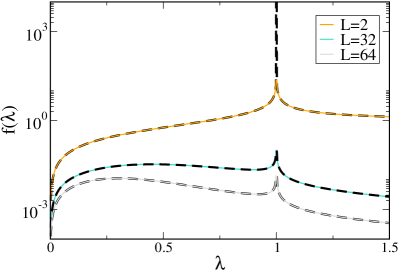
Figure 1: Comparison between the absolute values of LHS and RHS of the Eq. (8) for Hamiltonian Eq. (17) in solid lines and dashed lines respectively for different values of $L$.

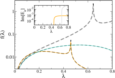
Figure 2: Comparison between the absolute value of LHS and RHS of the Eq. (8) for Hamiltonian Eq. (18) in solid lines and dashed lines respectively for $L=64$ and different eigenstates. Inset shows the imaginary part of those eigenvalues as a function of $\lambda$. Note that the cyan color plot is missing from the inset, that is because imaginary part of that eigenvalue is zero for $\lambda\leq 0.8$.

Next, we study $L\times L$ version of the above $2\times 2$, such Hamiltonian can be interpreted as a model of non-interacting fermions in 1D lattice with open boundary and described by the following Hamiltonian,

$${H_{0}}=-\sum_{j=1}^{L-1}(\hat{c}^{{\dagger}}_{j}\hat{c}_{j+1}+\text{H.c.})$$

(16)

where $\hat{c}^{{\dagger}}_{j}$ ($\hat{c}_{j}$) is the fermionic creation (annihilation) operator at site $j$, which satisfies standard anti-commutation relations. $L$ is the size of the system, which we set to be an even number for all our calculations ( we choose the lattice spacing as unity).

To make the Hamiltonian $PT$ symmetric and non-Hermitian, we add a local term at site $L/2$ and $L/2+1$. The $PT$ symmetric Hamiltonian reads as,

$$H_{L\times{L}}=H_{0}+i\lambda(\hat{n}_{L/2}-\hat{n}_{L/2+1})$$

(17)

where, $\hat{n}_{j}=\hat{c}^{{\dagger}}_{j}\hat{c}_{j}$ is the number operator and $\lambda$ is identified as the Hermiticity breaking parameter. While under Parity transformation $c_{j}\to c_{L-j+1}$, Time reversal symmetry operation changes $i\to-i$. Hence, $H_{L\times{L}}$ remains invariant under $PT$ transformation, which implies $[H_{L\times{L}},PT]=0$. For non-zero values of $\lambda$, $H_{L\times{L}}$ is non-Hermitian. For $L=2$, this model is identical to the two-level system we have studied previously. For any finite and even $L$ the Hamiltonian Eq. (17) shows a PT transition at $\lambda=1$ Modak and Mandal (2021). Like a two-level system, all eigenvalues are completely complex for $\lambda>1$. Note that it’s not necessary to have all eigenvalues to be complex in the PT broken phase; in contrast, we only need two of them to be complex. Fig. 1 shows excellent agreement between LHS and RHS of Eq. (8) (which we refer to as $f(\lambda)$). Interestingly, while Eq. (8) remains valid even when we approach towards EP i.e. $\lambda=1$, but the numerical value seems to diverge at EP. This is already clear for two-level systems from Eqs. (14) and (15), which diverge in the $\lambda\to 1$ limit. While this result is tempting to conclude that near EP LHS and RHS of Eq. (8) always diverges, it turns out to be not always true. Next, we study another model that is described by the Hamiltonian,

$$\tilde{H}_{L\times{L}}=H_{0}+i\lambda\sum_{j=L/2-(r-1)}^{L/2+r}(-1)^{j}\hat{n}_{j},$$

(18)

where we chose $r=2$. Hamiltonian Eq. (18) is interesting in the sense that in the PT broken phase of this model, not all eigenvalues are completely complex. A parameter regime exists when some eigenvalues are completely real, even in the broken phase. We find that while all eigenvalues and eigenstates modified HFT are valid, the divergence of LHS and RHS of Eq. (8) near EP occurs only for those eigenstates that show real to complex transition at EP. Eigenstates correspond to eigenvalues that remain real even after EP, for which no divergence has been observed at EP (see Fig. 2). We focus on three eigenstates of the Hamiltonian Eq. (18) for $L=64$ in Fig. 2 and also have plotted imaginary part of those eigenvalues as a function of $\lambda$. Note that while EP of this model corresponds to $\lambda_{c}\simeq 0.48$  Modak and Mandal (2021); Shukla et al. (2023), some states show no signature of divergence in $f(\lambda)$ at EP. However, it seems that $f(\lambda)$ tends to diverge when that eigenvalue also shows a real to complex transition. Hence, we conjecture the divergence of Eq. (8) is because of the real to complex transition of eigenvalues, and it explicitly has nothing to do with EP. Also, we believe that a variant of our lattice models with gain and loss is experimentally realizable in an ultracold fermionic system.

IV Continuum Model

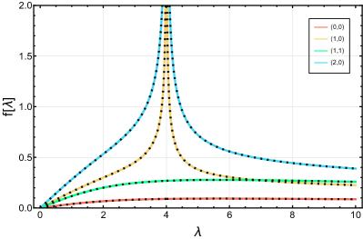
Figure 3: Comparison between the absolute value of $\Big{\langle}\frac{\partial\widehat{\mathcal{H}}}{\partial\lambda}\Big{\rangle}_{G}$ and $\frac{\partial{E_{n_{1},n_{2}}}}{\partial\lambda}$ for both broken and unbroken regions for the states $(n_{1},n_{2})=(0,0),(1,0),(1,1)$ and $(2,0)$. The solid lines and black dotted lines indicate the LHS and RHS of Eq. (22).

Now we consider the continuum model as an example; we take a 2-d anharmonic oscillator with a non-hermitian interaction term Mandal et al. (2013), which is described by

$$H_{2d}=\frac{p_{x}^{2}}{2m}+\frac{p_{y}^{2}}{2m}+\frac{1}{2}m\omega_{x}^{2}x^{2}+\frac{1}{2}m\omega_{y}^{2}y^{2}+i\lambda{xy},$$ (19)

where $\lambda$ is real and $\omega_{x}\neq\omega_{y}$. This system can be solved exactly. The energy eigenvalues and the right eigenvectors are given by,

$$R_{n_{1},n_{2}} = Ne^{-\frac{m}{2\hbar}\left[(C_{1}X^{2}+C_{2}Y^{2})\right]}H_{n_{1}}\left(\alpha_{1}X\right)H_{n_{2}}\left(\alpha_{2}Y\right)$$

$$E_{n_{1},n_{2}} = (n_{1}+\frac{1}{2})\hbar{C_{1}}+(n_{2}+\frac{1}{2})\hbar{C_{2}}$$ (20)

where, $\alpha_{1}=\sqrt{\frac{mC_{1}}{\hbar}}$ and $\alpha_{2}=\sqrt{\frac{mC_{2}}{\hbar}}$ and the left eigenvectors are given by,

$$L_{n_{1},n_{2}}=Ne^{-\frac{m}{2\hbar}\left[(C_{1}^{*}{X^{*}}^{2}+C_{2}^{*}{Y^{*}}^{2})\right]}H_{n_{1}}\left(\alpha_{1}^{*}X^{*}\right)H_{n_{2}}\left(\alpha_{2}^{*}Y^{*}\right)$$

where, $\alpha_{1}^{*}=\sqrt{\frac{mC_{1}^{*}}{\hbar}}$ and $\alpha_{2}^{*}=\sqrt{\frac{mC_{2}^{*}}{\hbar}}$

where,

$X=\sqrt{\frac{k+1}{2}}x-i\sqrt{\frac{k-1}{2}}y$

$Y=i\sqrt{\frac{k-1}{2}}x+\sqrt{\frac{k+1}{2}}y$. Moreover, $C_{1}=\sqrt{\frac{1}{2}\Big{(}\omega_{+}^{2}-\frac{\omega_{-}^{2}}{k}\Big{)}},\qquad{C_{2}=\sqrt{\frac{1}{2}\Big{(}\omega_{+}^{2}+\frac{\omega_{-}^{2}}{k}\Big{)}}}$

$\omega_{+}^{2}=\omega_{y}^{2}+\omega_{x}^{2},\qquad{\omega_{-}^{2}=\omega_{y}^{2}-\omega_{x}^{2}}$

$\frac{1}{k}=\sqrt{1-\frac{\lambda^{2}}{\lambda_{c}^{2}}}$ $\lambda_{c}=\frac{m\omega_{-}^{2}}{2}.$

The modified HFT in the case of continuum models is written in the integral form as,

$$\frac{\int{{\Big{(}L_{n_{1},n_{2}}^{*}}\Big{)}\frac{\partial{H_{2d}}}{\partial\lambda}\Big{(}R_{n_{1},n_{2}}\Big{)}dxdy}}{\int{{\Big{(}L_{n_{1},n_{2}}^{*}}\Big{)}\Big{(}R_{n_{1},n_{2}}\Big{)}dxdy}}=\frac{\partial{E_{n_{1},n_{2}}}}{\partial\lambda}.$$ (22)

It is straightforward to show that when $n_{1}=n_{2}$, the energy eigenvalues are real, and the eigenvectors are PT-symmetric over all values of $\lambda$. We have explicitly shown that the LHS and RHS of Eq. (22) are the same for ground state ( $n_{1}=n_{2}=0$) [ see Appendix B for details ].

Next we consider some of the low lying excited states. The energy eigenvalues can be real or complex depending on the value of $\lambda$. We have plotted the absolute value of LHS and RHS of the modified HFT for all these states in Fig. 3 to check the validity of the theorem. Note that we have also checked explicitly for $(1,0),(2,0)$, the real and imaginary parts of the LHS and RHS of the Eq. (22) separately (see Appendix B). We also find that $f(\lambda)$ for the 1st excited state diverges near $\lambda=4$ and at the same value of $\lambda$ the eigenvalue of the 1st excited state also shows real to complex transition. This result strengthens our previous claim, i.e., the divergence of $f(\lambda)$ corresponds to the real to the complex transition of the eigenvalues.

V Virial theorem for non-Hermitian system

A generalized virial theorem has been derived for $N$ particles quantum system Werner (2008), with arbitrary statistics and dispersion relations. One can consider a general Hamiltonian,

$$\widehat{\mathcal{H}}=\widehat{\mathcal{H}}^{\prime}+U(r_{1},...,r_{N})$$ (23)

where $\widehat{\mathcal{H}}^{\prime}$ and its domain depend on p parameters $l_{1},...,l_{p}$ which have the dimension of a length, and $U(r_{1},...,r_{N})$ is an arbitrary function, where $r_{i}$ is the position of particle $i$. Using HFT for the Hermitian system, it has been shown in Ref. Werner (2008) that for any stationary state energy $E$ the following relation holds,

$$E=\left\langle{U+\frac{1}{2}\sum_{i=1}^{N}{r_{i}}.\nabla{U\left(r_{i}\right)}}\right\rangle-\frac{1}{2}\sum_{q=1}^{p}l_{q}{\frac{\partial E}{\partial l_{q}}}.$$ (24)

If $\widehat{\mathcal{H}}$ is non-Hermitian, it is straightforward to derive a generalized version of the virial theorem using the modified HFT. It just reads as,

$$E=\left\langle{U+\frac{1}{2}\sum_{i=1}^{N}{r_{i}}.\nabla{U\left(r_{i}\right)}}\right\rangle_{G}-\frac{1}{2}\sum_{q=1}^{p}l_{q}{\frac{\partial E}{\partial l_{q}}}.$$ (25)

Next, we take a concrete example of 1D non-Hermitian harmonic oscillator with complex angular frequency; the Hamiltonian reads as,

$$H_{1d}=\frac{p^{2}}{2}+\frac{1}{2}\Omega^{2}x^{2}$$ (26)

where, $\Omega=\omega_{1}+i\omega_{2}$ and $\omega_{1}\neq 0$. Note that this Hamiltonian is not PT invariant. However, given our modified HFT holds even for the Hamiltonian, which is not PT invariant, one can still use the modified HFT to derive the generalized virial theorem Eq. (25).

The trapping energy for such a non-hermitian system is given by

$$\tilde{E}_{tr}=\frac{1}{2}\left\langle{U\left(x\right)+\frac{1}{2}{x}.\nabla_{x}{U\left(x\right)}}\right\rangle_{G}$$ (27)

We have,

$$U=\frac{1}{2}\Omega^{2}x^{2}$$ (28)

Therefore, Eq. (27) implies,

$$\tilde{E}_{tr}=\frac{1}{2}\left\langle{\frac{1}{2}\Omega^{2}x^{2}+\frac{1}{2}{x}.\nabla{\left(\frac{1}{2}\Omega^{2}x^{2}\right)}}\right\rangle_{G}$$

$$=\frac{1}{2}\left\langle{\Omega^{2}x^{2}}\right\rangle_{G}$$ (29)

Using the definition of the G-inner product given in Eq. (4), we will now deduce Eq. (V) for the ground state and all the excited states. For ground state,

Left eigenvector of $H_{1d}$ is given by

$$L_{0}={\left(\frac{\omega_{1}-i\omega_{2}}{\pi}\right)}^{\frac{1}{4}}e^{-\frac{\omega_{1}{x^{2}}}{2}}e^{\frac{i\omega_{2}{x^{2}}}{2}}$$ (30)

and right eigenvector of $H_{1d}$ is given by

$$R_{0}={\left(\frac{\omega_{1}+i\omega_{2}}{\pi}\right)}^{\frac{1}{4}}e^{-\frac{\omega_{1}{x^{2}}}{2}}e^{-\frac{i\omega_{2}{x^{2}}}{2}}.$$ (31)

Therefore, Eq. (V) implies,

$$\tilde{E}_{tr_{0}}= \frac{\int{{\Big{(}L_{0}^{*}}\Big{)}{\frac{1}{2}\Omega^{2}x^{2}}\Big{(}R_{0}\Big{)}dx}}{\int{{\Big{(}L_{0}^{*}}\Big{)}\Big{(}R_{0}\Big{)}dx}}$$

$$= \frac{\int{e^{-\omega_{1}{x^{2}}}e^{-i\omega_{2}{x^{2}}}{\frac{1}{2}\Omega^{2}x^{2}}dx}}{\int{e^{-\omega_{1}{x^{2}}}e^{-i\omega_{2}{x^{2}}}dx}}$$

$$= \frac{1}{4}\Omega=\frac{1}{2}E_{0},$$ (32)

where $E_{0}$ is the ground state energy of the Hamiltonian Eq. (26).

One can also compute trapping energy for the $n^{th}$ eigenstate. we have,

$$x=\frac{1}{\sqrt{2\Omega}}\left(a^{\dagger}+a\right)$$ (33)

and

$$p=i\sqrt{\frac{\Omega}{2}}\left(a^{\dagger}-a\right)$$ (34)

such that

$$a|n\rangle=\sqrt{n}|n-1\rangle\quad\text{and}\quad a^{\dagger}|n\rangle=\sqrt{n+1}|n+1\rangle$$ (35)

where, $|n\rangle$ is the $n^{th}$ state of $H_{1d}$, also, the right eigenvector, $|R_{n}\rangle$ of $H_{1d}$, $\left(i.e.,|R_{n}\rangle=|n\rangle\right)$.

Similarly,

$$H_{1d}^{\dagger}=\frac{p^{2}}{2}+\frac{1}{2}{\Omega^{*}}^{2}x^{2},$$ (36)

and we have,

$$x=\frac{1}{\sqrt{2\Omega^{*}}}\left(b^{\dagger}+b\right)$$ (37)

and

$$p=i\sqrt{\frac{\Omega^{*}}{2}}\left(b^{\dagger}-b\right)$$ (38)

such that

$$b|\bar{n}\rangle=\sqrt{\bar{n}}|\bar{n}-1\rangle\quad\text{and}\quad b^{\dagger}|\bar{n}\rangle=\sqrt{\bar{n}+1}|\bar{n}+1\rangle$$ (39)

where, $|\bar{n}\rangle$ is the $\bar{n}^{th}$ state of $H_{1d}^{\dagger}$, also, the left eigenvector, $|L_{n}\rangle$ of $H_{1d}$, $\left(i.e.,|L_{n}\rangle=|\bar{n}\rangle\right)$.

Therefore, by using Eq. (4), we can derive the trapping energy for $n^{th}$-eigenstate as,

$$\tilde{E}_{tr_{n}}= \langle{L_{n}}|\frac{1}{2}\Omega^{2}x^{2}|R_{n}\rangle=\langle{\bar{n}}|\frac{1}{2}\Omega^{2}x^{2}|n\rangle$$

$$= \frac{1}{2}\Omega^{2}\left(\frac{1}{2\Omega}\right)\langle{\bar{n}}|{a^{\dagger}}^{2}+a^{2}+a^{\dagger}a+aa^{\dagger}|n\rangle$$

$$= \frac{\Omega}{4}\langle{\bar{n}}|2n+1|n\rangle$$

$$= \frac{1}{2}\left(n+\frac{1}{2}\right)\Omega=\frac{1}{2}E_{n},$$ (40)

where $E_{n}$ corresponds to eigenenergy of the $n^{th}$ state. The relation between the energy eigenvalue and the trapping energy is the same even for the Hermitian harmonic oscillator.

VI Conclusions

In this work, we derive the modified HFT for the non-Hermitian system. Our modified HFT works for both PT-invariant and non-invariant systems. The derivation is extremely general. However, given the Hamiltonian is a good observable in the PT-symmetric phase of the PT invariant system, only in that phase the LHS and RHS of the modified HFT in Eq. (8) guaranteed to be completely real. Moreover, if the eigenvalue goes through a real to complex transition as a function of the Hermiticity breaking parameter, the LHS and RHS of the modified HFT diverge at that point. If that point is an EP of the PT invariant quantum theory, then one sees the divergence at EP as well; otherwise, both sides of Eq. (8) can be finite at EP as well. We test our results for different discrete and continuum models; some of those models have already been experimentally realized and have a huge technological application as a quantum sensor Yu et al. (2020).

Finally, we also derive a generalized Virial theorem for non-Hermitian systems and show that for a Harmonic oscillator with complex frequency, the system’s energy is twice the trapping energy, precisely what one observes for a Hermitian Harmonic oscillator. For the Hermitian system, the trapping potential energy $E_{tr}$ has been computed from the density profile Bartenstein et al. (2004); den , and the released energy $E-E_{tr}$ from a time-of-flight experiment Bourdel et al. (2004). Note that recently there has been an experimental proposal to compute the G-inner product for a non-Hermitian system using weak measurement Huang et al. (2019); we believe the same strategy can be used to compute both energy and trapping energy of the non-Hermitian system; hence experimental verification of Virial theorem for the non-Hermitian system should be possible. Moreover, given that DNA-unzipping transition can be effectively described by a non-Hermitian Hatano-Nelson model  Pal et al. (2022); Hatano and Nelson (1996), it will be interesting in future to compute the critical force for DNA-unzipping transition using the modified HFT.

Acknowledgements: RM acknowledges the DST-Inspire fellowship by the Department of Science and Technology, Government of India, SERB start-up grant (SRG/2021/002152). BPM acknowledges the research grant for faculty under IoE Scheme (Number 6031) of Banaras Hindu University, Varanasi. GH acknowledges the UGC-JRF Fellowship

Appendix A Four level System

We consider a particular $4\times 4$ non-Hermitian Hamiltonian as Modak and Mandal (2021),

$$H_{4\times{4}}=\begin{pmatrix}{i\lambda}&{-1}&{0}&{0}\\ {-1}&{-i\lambda}&{-1}&{0}\\ {0}&{-1}&{i\lambda}&{-1}\\ {0}&{0}&{-1}&{-i\lambda}\end{pmatrix}$$

The eigenvalues and right eigenfunctions for this system are calculated as
$E_{1}=-\sqrt{\frac{3-\sqrt{5}-2\lambda^{2}}{2}},\quad{E_{2}=\sqrt{\frac{3-\sqrt{5}-2\lambda^{2}}{2}}},\quad{E_{3}=-\sqrt{\frac{3+\sqrt{5}-2\lambda^{2}}{2}}},\quad{E_{4}=\sqrt{\frac{3+\sqrt{5}-2\lambda^{2}}{2}}}$ and

$$|R_{1}\rangle=\begin{pmatrix}{u_{1_{-}}}\\ {v_{1}}\\ w_{1_{+}}\\ 1\end{pmatrix},\quad|R_{2}\rangle=\begin{pmatrix}{u_{1_{+}}}\\ {v_{1}}\\ w_{1_{-}}\\ 1\end{pmatrix},\quad|R_{3}\rangle=\begin{pmatrix}{u_{2_{-}}}\\ {v_{2}}\\ w_{2_{+}}\\ 1\end{pmatrix},\quad|R_{4}\rangle=\begin{pmatrix}{u_{2_{+}}}\\ {v_{2}}\\ w_{2_{-}}\\ 1\end{pmatrix}$$

where,

$$u_{1_{\pm}}=\frac{1}{4}\left(2i\lambda\left(1+\sqrt{5}\right)\pm\left(\sqrt{2}+\sqrt{10}\right)\sqrt{3-\sqrt{5}-2\lambda^{2}}\right),$$

$${u_{2_{\pm}}}=\frac{1}{4}\left(2i\lambda\left(1-\sqrt{5}\right)\pm\left(\sqrt{2}-\sqrt{10}\right)\sqrt{3+\sqrt{5}-2\lambda^{2}}\right),$$

$${v_{1}}=\frac{\left(1-\sqrt{5}\right)}{2},\quad{v_{2}}=\frac{\left(1+\sqrt{5}\right)}{2},$$

$${w_{1_{\pm}}}=-i\lambda\pm\sqrt{\frac{3-\sqrt{5}-2\lambda^{2}}{2}},\quad{w_{2_{\pm}}}=-i\lambda\pm\sqrt{\frac{3+\sqrt{5}-2\lambda^{2}}{2}}.$$ (41)

We observe that if $\lambda<\lambda_{C_{1}}=\sqrt{\frac{3-\sqrt{5}}{2}},$ then all eigenvalues are real and if $\lambda_{C_{1}}<\lambda<\lambda_{C_{2}}=\sqrt{\frac{3+\sqrt{5}}{2}},$ then two of the eigenvalues are real and two are complex conjugate pair. For $\lambda>\lambda_{C_{2}},$ all four eigenvalues are complex. It can be shown that the system is in the unbroken phase for $\lambda<\lambda_{C_{1}}$.

We calculate the G metric in the unbroken phase using Eq. (3) as,

$$G^{u}=\frac{1}{10\left(1-3\lambda^{2}+\lambda^{4}\right)}\begin{bmatrix}3-2\lambda^{2}&{i\lambda\left(3-2\lambda^{2}\right)}&-{\left(\lambda^{2}+1\right)}&{i\lambda\left(\lambda^{2}-4\right)}\\ {i\lambda\left(2\lambda^{2}-3\right)}&{2-3\lambda^{2}}&{i\left(\lambda^{3}+\lambda\right)}&-{\left(\lambda^{2}+1\right)}\\ -{\left(\lambda^{2}+1\right)}&-{i\left(\lambda^{3}+\lambda\right)}&{2-3\lambda^{2}}&{i\lambda\left(3-2\lambda^{2}\right)}\\ -{i\lambda\left(\lambda^{2}-4\right)}&-{\left(\lambda^{2}+1\right)}&{i\lambda\left(2\lambda^{2}-3\right)}&{3-2\lambda^{2}}\end{bmatrix}$$

We explicitly check that $|R_{1}\rangle$ satisfies the modified HFT relation in Eq. (9):

$$\frac{\partial{E_{1}}}{\partial\lambda}=\frac{\partial}{\partial{\lambda}}\left(-\sqrt{\frac{3-\sqrt{5}-2\lambda^{2}}{2}}\right)=\frac{\sqrt{2}\lambda}{\sqrt{3-\sqrt{5}-2\lambda^{2}}}$$ (42)

We further calculate

$$\Big{\langle}{R_{1}}\Big{|}G^{u}\frac{\partial{H_{4\times{4}}}}{\partial\lambda}\Big{|}R_{1}\Bigr{\rangle}=\frac{\sqrt{2}\lambda}{\sqrt{3-\sqrt{5}-2\lambda^{2}}},$$ (43)

to establish the modified HFT for the state $|R_{1}\rangle$,

$$\boxed{\Big{\langle}{R_{1}}\Big{|}G^{u}\frac{\partial{H_{4\times{4}}}}{\partial\lambda}\Big{|}R_{1}\Bigr{\rangle}=\frac{\partial{E_{1}}}{\partial\lambda}}$$

In the similar way, it can be shown that other states also satisfy the modified HFT.

Now we consider the system in the broken phase, when $\lambda_{C_{1}}<\lambda<\lambda_{C_{2}}$. The eigenvalues in this region are, $E_{1}^{\prime}=-i\sqrt{\frac{-3+\sqrt{5}+2\lambda^{2}}{2}},\quad{E_{2}^{\prime}=i\sqrt{\frac{-3+\sqrt{5}+2\lambda^{2}}{2}}},\quad{E_{3}^{\prime}=-\sqrt{\frac{3+\sqrt{5}-2\lambda^{2}}{2}}},\quad{E_{4}^{\prime}=\sqrt{\frac{3+\sqrt{5}-2\lambda^{2}}{2}}}$

The G metric in this region of coupling $\lambda$ is calculated as

$$G^{b}_{1}=\frac{1}{10\left(1-3\lambda^{2}+\lambda^{4}\right)}\begin{bmatrix}-\sqrt{5}&{-i\lambda\sqrt{5}}&{-\sqrt{5}\left(\lambda^{2}-1\right)}&-{i\lambda\sqrt{5}\left(\lambda^{2}-2\right)}\\ {i\lambda\sqrt{5}}&{2-\left(6+\sqrt{5}\right)\lambda^{2}+2\lambda^{4}}&{i\lambda\left(\lambda^{2}-1\right)}&g_{2,4}\\ {-\sqrt{5}\left(\lambda^{2}-1\right)}&-{i\lambda\left(\lambda^{2}-1\right)}&{-\sqrt{5}\lambda^{2}}&{-i\lambda\sqrt{5}}\\ {i\lambda\sqrt{5}\left(\lambda^{2}-2\right)}&g_{4,2}&{i\lambda\sqrt{5}}&g_{4,4}\end{bmatrix}$$

where, $g_{4,2}=g_{2,4}=-1+\left(3+2\sqrt{5}\right)\lambda^{2}-\left(1+\sqrt{5}\right)\lambda^{4}$ and $g_{4,4}={3+\left(3+\sqrt{5}\right)\lambda^{2}\left(-3+\lambda^{2}\right)}$

We find that the states in this broken region also satisfy the modified HFT relation ( Eq. (12)):

$$\frac{\partial{E_{1}^{\prime}}}{\partial\lambda}=\frac{\partial}{\partial{\lambda}}\left(-i\sqrt{\frac{-3+\sqrt{5}+2\lambda^{2}}{2}}\right)=-\frac{i\sqrt{2}\lambda}{\sqrt{-3+\sqrt{5}+2\lambda^{2}}}$$ (44)

and,

$$\Big{\langle}{R_{1}}\Big{|}G^{b}_{1}\frac{\partial{H_{4\times{4}}}}{\partial\lambda}\Big{|}R_{1}\Bigr{\rangle}=-\frac{i\sqrt{2}\lambda}{\sqrt{-3+\sqrt{5}+2\lambda^{2}}}=\frac{\partial{E_{1}^{\prime}}}{\partial\lambda}$$ (45)

implying that,

$$\boxed{\Big{\langle}{R_{1}}\Big{|}G^{b}_{1}\frac{\partial{H_{4\times{4}}}}{\partial\lambda}\Big{|}R_{1}\Bigr{\rangle}=\frac{\partial{E_{1}^{{}^{\prime}}}}{\partial\lambda}}$$

In the similar straightforward manner other states can be shown to satisfy the modified HFT in this broken region.

Finally, we consider the region $\lambda>\lambda_{C_{2}},$ where all eigenvalues are complex. The eigenvalues in this region are calculated as, $E_{1}^{\prime\prime}=-i\sqrt{\frac{-3+\sqrt{5}+2\lambda^{2}}{2}},\quad{E_{2}{\prime\prime}=i\sqrt{\frac{-3+\sqrt{5}+2\lambda^{2}}{2}}},\quad{E_{3}^{\prime\prime}=-i\sqrt{\frac{-3-\sqrt{5}+2\lambda^{2}}{2}}},\quad{E_{4}^{\prime\prime}=i\sqrt{\frac{-3-\sqrt{5}+2\lambda^{2}}{2}}}$. The G metric is constructed as,

$$G^{b}_{2}=\frac{1}{10\left(1-3\lambda^{2}+\lambda^{4}\right)}\begin{bmatrix}-3+2\lambda^{2}&{i\lambda\left(-3+2\lambda^{2}\right)}&{\left(\lambda^{2}+1\right)}&-{i\lambda\left(\lambda^{2}-4\right)}\\ {i\lambda\left(-2\lambda^{2}+3\right)}&{2-9\lambda^{2}+4\lambda^{4}}&-{i\left(\lambda^{3}+\lambda\right)}&-1+7\lambda^{2}-2\lambda^{4}\\ {\left(\lambda^{2}+1\right)}&{i\left(\lambda^{3}+\lambda\right)}&{-2+3\lambda^{2}}&{i\lambda\left(-3+2\lambda^{2}\right)}\\ {i\lambda\left(\lambda^{2}-4\right)}&-1+7\lambda^{2}-2\lambda^{4}&{i\lambda\left(-2\lambda^{2}+3\right)}&{3-16\lambda^{2}+6\lambda^{4}}\end{bmatrix}$$

We now check below that $|R_{1}\rangle$ still satisfies the modified HFT relation as given in Eq. (12): The LHS of modified HFT is

$$\frac{\partial{E_{1}^{\prime\prime}}}{\partial\lambda}=\frac{\partial}{\partial{\lambda}}\left(-i\sqrt{\frac{-3+\sqrt{5}+2\lambda^{2}}{2}}\right)=-\frac{i\sqrt{2}\lambda}{\sqrt{-3+\sqrt{5}+2\lambda^{2}}}$$ (46)

which is exactly equal to the RHS of the modified HFT.

$$\Big{\langle}{R_{1}}\Big{|}G^{b}_{2}\frac{\partial{H_{4\times{4}}}}{\partial\lambda}\Big{|}R_{1}\Bigr{\rangle}=-\frac{i\sqrt{2}\lambda}{\sqrt{-3+\sqrt{5}+2\lambda^{2}}}=\frac{\partial{E_{1}^{\prime\prime}}}{\partial\lambda}$$ (47)

The same is true for all other states. This establishes the verification of the modified HFT for $4\times 4$ system in broken and unbroken phases.

Appendix B HFT for 2-d anharmonic oscillator with non-Hermitian interaction

We consider the 2-d anharmonic oscillator as described in Eq. (19). We choose the following numerical values for different parameters, $\omega_{x}=1,\quad\omega_{y}=3,\quad\hbar=1,\quad{m}=1$ for the numerical computations. The critical coupling $\lambda_{c}=\frac{m\omega_{-}^{2}}{2}$ becomes 4.

• For unbroken region $(\lambda<\lambda_{c})$:

  $$k^{*}=k;\ \ C_{1}^{*}=C_{1},\ C_{2}^{*}=C_{2};\ \ \alpha_{1}^{*}=\alpha_{1},\ \alpha_{2}^{*}=\alpha_{2}$$ (48)

  $$X^{*}=\sqrt{\frac{k+1}{2}}x+i\sqrt{\frac{k-1}{2}}y$$ (49)

  $$Y^{*}=-i\sqrt{\frac{k-1}{2}}x+\sqrt{\frac{k+1}{2}}y$$ (50)

• For broken region $(\lambda>\lambda_{c})$:

  $$k^{*}=-k;\ \ C_{1}^{*}=C_{2}=A+iB;\ \ \alpha_{1}^{*}=\alpha_{2},\ \ \alpha_{2}^{*}=\alpha_{1}$$ (51)

  $$X^{*}=i\sqrt{\frac{k-1}{2}}x-\sqrt{\frac{k+1}{2}}y$$ (52)

  $$Y^{*}=\sqrt{\frac{k+1}{2}}x+i\sqrt{\frac{k-1}{2}}y$$ (53)

  with

  $$A=\frac{1}{2}\sqrt{\sqrt{\frac{\omega_{-}^{4}}{k_{1}^{2}}+\omega_{+}^{4}}+\omega_{+}^{2}};\ \ B=\frac{1}{2}\sqrt{\sqrt{\frac{\omega_{-}^{4}}{k_{1}^{2}}+\omega_{+}^{4}}-\omega_{+}^{2}};\ \ \mbox{and }k_{1}=ik$$ (54)

1. Now for ground state $n_{1}=0,n_{2}=0,$ the energy eigenvalues $E_{0,0}$ are always real for all values of $\lambda$, suggesting that there is no broken phase. We have calculated LHS and RHS of modified HFT analytically to show the equivalence. Using Eqs. (48) to (50), the Eqs. (IV) and (IV) are rewritten as,

   $$R_{0,0} = Ne^{-\frac{1}{4}\big{[}(C_{1}+C_{2})(x^{2}+y^{2})+(C_{2}-C_{1})\big{\{}\frac{2i\lambda{kxy}}{\lambda_{c}}-k(x^{2}-y^{2})\big{\}}\big{]}}$$ (55)

   $$L_{0,0} = Ne^{-\frac{1}{4}\big{[}(C_{1}+C_{2})(x^{2}+y^{2})+(C_{1}-C_{2})\left\{\frac{2i\lambda{kxy}}{\lambda_{c}}+k(x^{2}-y^{2})\right\}\big{]}},$$ (56)

   Now, we proceed to verify the modified HFT, using Eqs. (55) and (56) the LHS of Eq. (22) implies,

   $$\Big{\langle}\frac{\partial{H_{2d}}}{\partial\lambda}\Big{\rangle}_{G,(0,0)}=\frac{\int{{\Big{(}L_{0,0}^{*}}\Big{)}\frac{\partial{H_{2d}}}{\partial\lambda}\Big{(}R_{0,0}\Big{)}dxdy}}{\int{{\Big{(}L_{0,0}^{*}}\Big{)}\Big{(}R_{0,0}\Big{)}dxdy}}$$

   $$=\frac{|N|^{2}\int{ixye^{-\frac{m}{2\hbar}\big{[}(C_{1}+C_{2})(x^{2}+y^{2})+(C_{2}-C_{1})\big{\{}\frac{2i\lambda{kxy}}{\lambda_{c}}-k(x^{2}-y^{2})\big{\}}\big{]}}dxdy}}{|N|^{2}\int{e^{-\frac{m}{2\hbar}\big{[}(C_{1}+C_{2})(x^{2}+y^{2})+(C_{2}-C_{1})\big{\{}\frac{2i\lambda{kxy}}{\lambda_{c}}-k(x^{2}-y^{2})\big{\}}\big{]}}dxdy}}$$

   $$=-\frac{\lambda\left(\lambda^{2}-4\sqrt{\lambda^{2}+9}+4\right)\sqrt{5-\sqrt{16-\lambda^{2}}}}{\left(16-\lambda^{2}\right)\left(\lambda^{2}+8\right)\sqrt{\lambda^{2}+9}}-\frac{\lambda\left(\lambda^{2}-4\sqrt{\lambda^{2}+9}+4\right)\sqrt{5-\sqrt{16-\lambda^{2}}}}{4\sqrt{16-\lambda^{2}}\left(\lambda^{2}+8\right)\sqrt{\lambda^{2}+9}}$$

   $$+\frac{\lambda\left(\lambda^{2}-4\sqrt{\lambda^{2}+9}+4\right)\sqrt{\sqrt{16-\lambda^{2}}+5}}{4\sqrt{16-\lambda^{2}}\left(\lambda^{2}+8\right)\sqrt{\lambda^{2}+9}}-\frac{\lambda\left(\lambda^{2}-4\sqrt{\lambda^{2}+9}+4\right)\sqrt{\sqrt{16-\lambda^{2}}+5}}{\left(16-\lambda^{2}\right)\left(\lambda^{2}+8\right)\sqrt{\lambda^{2}+9}}$$ (57)

   RHS of Eq. (22) for the $(0,0)$ state is,

   $$\frac{\partial{E_{0,0}}}{\partial\lambda}=\frac{\partial}{\partial\lambda}\Big{(}\frac{1}{2}{C_{1}}+\frac{1}{2}{C_{2}}\Big{)}=\frac{\lambda\sqrt{\sqrt{\lambda^{2}+9}-5}}{2\sqrt{2}\sqrt{\lambda^{2}-16}\sqrt{\lambda^{2}+9}}$$ (58)

   The RHS of the Eqs. (1) and (58) are same for all values of $\lambda$, as shown in Fig. 4, indicating that modified HFT is valid for the ground state $n_{1}=n_{2}=0$, for all values of $\lambda$.

   

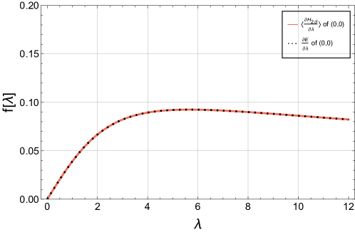
   Figure 4: Comparison between $\Big{\langle}\frac{\partial{H_{2d}}}{\partial\lambda}\Big{\rangle}_{G,(0,0)}$ and $\frac{\partial{E_{0,0}}}{\partial\lambda}$, represented by the solid and the dotted lines respectively.

2. First excited state: $n_{1}=1,n_{2}=0$.

   • Unbroken phase: $\lambda<\lambda_{c}$

     Using the relations in Eqs. (48) to (50), the right and the left eigenvectors are derived as,

     $$R_{1,0} = Ne^{-\frac{1}{4}\big{[}(C_{1}+C_{2})(x^{2}+y^{2})+(C_{2}-C_{1})\big{\{}\frac{2i\lambda{kxy}}{\lambda_{c}}-k(x^{2}-y^{2})\big{\}}\big{]}}2\alpha_{1}\left(\sqrt{\frac{k+1}{2}}x-i\sqrt{\frac{k-1}{2}y}\right)$$ (59)

     $$L_{1,0} = Ne^{-\frac{1}{4}\big{[}(C_{1}+C_{2})(x^{2}+y^{2})+(C_{1}-C_{2})\big{\{}\frac{2i\lambda{kxy}}{\lambda_{c}}+k(x^{2}-y^{2})\big{\}}\big{]}}2\alpha_{1}\left(\sqrt{\frac{k+1}{2}}x+i\sqrt{\frac{k-1}{2}y}\right)$$ (60)

     with the common eigenvalue, $\quad\quad{E_{1,0}^{*}}=E_{1,0}=(\frac{3}{2}){C_{1}}+(\frac{1}{2}){C_{2}}$. Hence, the LHS of modified HFT is,

     $$\Big{\langle}\frac{\partial{H_{2d}}}{\partial\lambda}\Big{\rangle}_{G,(1,0)}=\frac{\int{{\Big{(}L_{1,0}^{*}}\Big{)}\frac{\partial{H_{2d}}}{\partial\lambda}\Big{(}R_{1,0}\Big{)}dxdy}}{\int{{\Big{(}L_{1,0}^{*}}\Big{)}\Big{(}R_{1,0}\Big{)}dxdy}}$$

     $$=\frac{|N|^{2}\int{ixyc_{1}\left(\sqrt{\frac{k+1}{2}}x-i\sqrt{\frac{k-1}{2}}y\right)^{2}e^{-\frac{1}{2}\big{[}(C_{1}+C_{2})(x^{2}+y^{2})+(C_{2}-C_{1})\big{\{}\frac{2i\lambda{kxy}}{\lambda_{c}}-k(x^{2}-y^{2})\big{\}}\big{]}}dxdy}}{|N|^{2}\int{c_{1}\left(\sqrt{\frac{k+1}{2}}x-i\sqrt{\frac{k-1}{2}}y\right)^{2}e^{-\frac{1}{2}\big{[}(C_{1}+C_{2})(x^{2}+y^{2})+(C_{2}-C_{1})\big{\{}\frac{2i\lambda{kxy}}{\lambda_{c}}-k(x^{2}-y^{2})\big{\}}\big{]}}dxdy}}$$ (61)

     And the RHS of modified HFT is,

     $$\frac{\partial{E_{1,0}}}{\partial\lambda}=\frac{\partial}{\partial\lambda}\Big{(}\frac{3}{2}{C_{1}}+\frac{1}{2}{C_{2}}\Big{)}=\frac{3\lambda}{8\sqrt{2\left(1-\frac{\lambda^{2}}{16}\right)\left(10-8\sqrt{1-\frac{\lambda^{2}}{16}}\right)}}-\frac{\lambda}{8\sqrt{2\left(1-\frac{\lambda^{2}}{16}\right)\left(10+8\sqrt{1-\frac{\lambda^{2}}{16}}\right)}}$$ (62)

     The expressions in the RHS of the Eqs. (61) and (62) in the domain $\lambda<\lambda_{c}(=4)$ are equal as shown in Fig. 3, indicating that the modified HFT is valid for the state $(n_{1}=1,n_{2}=0)$ in the unbroken case.

   • Broken phase: $\lambda>\lambda_{c}$

     Using the relations in Eqs. (51) to (53), the right and the left eigenvectors are calculated along with their eigenvalues as,

     $$R_{1,0}=Ne^{-\frac{1}{4}\big{[}2A(x^{2}+y^{2})+2iB\big{\{}\frac{2i\lambda{kxy}}{\lambda_{c}}-k(x^{2}-y^{2})\big{\}}\big{]}}2\alpha_{1}\left(\sqrt{\frac{k+1}{2}}x-i\sqrt{\frac{k-1}{2}}y\right)$$ (63)

     $${E_{1,0}}=\frac{3}{2}{C_{1}}+\frac{1}{2}{C_{2}}=\frac{3}{2}{(A-iB)}+\frac{1}{2}{(A+iB)}=2A-iB$$ (64)

     And,

     $$L_{1,0}=Ne^{-\frac{1}{4}\big{[}2A(x^{2}+y^{2})-2iB\big{\{}\frac{2i\lambda{kxy}}{\lambda_{c}}+k(x^{2}-y^{2})\big{\}}\big{]}}2\alpha_{1}^{*}\left(i\sqrt{\frac{k-1}{2}}x-\sqrt{\frac{k+1}{2}}y\right)$$ (65)

     with eigenvalue $E_{1,0}^{*}$. The LHS of the modified HFT is calculated as,

     $$\Big{\langle}\frac{\partial{H_{2d}}}{\partial\lambda}\Big{\rangle}_{G,(1,0)} = \frac{\int{{\Big{(}L_{1,0}^{*}}\Big{)}\frac{\partial{H_{2d}}}{\partial\lambda}\Big{(}R_{1,0}\Big{)}dxdy}}{\int{{\Big{(}L_{1,0}^{*}}\Big{)}\Big{(}R_{1,0}\Big{)}dxdy}}$$ (66)

     $$= \frac{|N|^{2}\int{ixyc_{1}\left(\sqrt{\frac{k+1}{2}}x-i\sqrt{\frac{k-1}{2}}y\right)^{2}e^{-\frac{1}{2}\big{[}2A(x^{2}+y^{2})+i2B\big{\{}\frac{2i\lambda{kxy}}{\lambda_{c}}-k(x^{2}-y^{2})\big{\}}\big{]}}dxdy}}{|N|^{2}\int{c_{1}\left(\sqrt{\frac{k+1}{2}}x-i\sqrt{\frac{k-1}{2}}y\right)^{2}e^{-\frac{1}{2}\big{[}2A(x^{2}+y^{2})+i2B\big{\{}\frac{2i\lambda{kxy}}{\lambda_{c}}-k(x^{2}-y^{2})\big{\}}\big{]}}dxdy}}$$

     RHS of modified HFT is,

     $$\frac{\partial{E_{1,0}}}{\partial\lambda}=\frac{\partial}{\partial\lambda}\Big{(}2A-iB\Big{)}$$ (67)

     $$= \frac{2\lambda}{\sqrt{64\left(\frac{\lambda^{2}}{16}-1\right)+100}\sqrt{\sqrt{64\left(\frac{\lambda^{2}}{16}-1\right)+100}+10}}-\frac{i\lambda}{\sqrt{64\left(\frac{\lambda^{2}}{16}-1\right)+100}\sqrt{\sqrt{64\left(\frac{\lambda^{2}}{16}-1\right)+100}-10}}$$

     The imaginary and the real parts of the relations given by Eqs. (66) and (67) over the broken region are shown in Fig. 5. We have also shown the real and imaginary parts of Eq. (22) for $(2,0)$ state in the same figure in order to compare it with the $(1,0)$ state. We find that the curves representing the LHS and RHS of Eq. (22) completely overlap each other for both $(1,0)$ and $(2,0)$ states, indicating the validity of the modified HFT for these states as well.

     

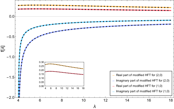
     Figure 5: Comparison between real and imaginary parts of $\Big{\langle}\frac{\partial{H_{2d}}}{\partial\lambda}\Big{\rangle}_{G,(1,0)}$ and $\Big{\langle}\frac{\partial{H_{2d}}}{\partial\lambda}\Big{\rangle}_{G,(2,0)}$ with that of $\frac{\partial{E_{1,0}}}{\partial\lambda}$ and $\frac{\partial{E_{2,0}}}{\partial\lambda}$ in the broken region. Colored solid lines and black dotted lines represent the LHS and RHS of modified HFT respectively.

Appendix C HFT for non-PT invariant non-Hermitian system

We consider here a simple 1-d Hamiltonian( Eq. (26))representing non-PT symmetric non-hermitian system

$$H_{1d}=\frac{p^{2}}{2}+\frac{1}{2}\Omega^{2}x^{2}.$$ (68)

where, $\Omega=\omega_{1}+i\omega_{2}$ and $\omega_{1,2}$ are real and $\omega_{1,2}\neq 0.$

We intend to verify the modified HFT

$$\Big{\langle}\frac{\partial{H_{1d}}}{\partial\lambda}\Big{\rangle}_{G,(n)}=\frac{\partial{E_{n}}}{\partial\lambda}$$ (69)

for the above system for an arbitrary $n^{th}$ state with 3 different choices of $\lambda:$

1. First choice, $\lambda=\omega_{1}$: Considering the relations in equations from Eqs. (33) to (35), we can write,

   $$\Big{\langle}\frac{\partial{H_{1d}}}{\partial\omega_{1}}\Big{\rangle}_{G,(n)}=\langle{\bar{n}}|\Omega{x^{2}}|n\rangle=\frac{1}{2}\langle{\bar{n}}|{a^{+}}^{2}+a^{2}+a^{+}a+aa^{+}|n\rangle=\frac{1}{2}\langle{\bar{n}}|2n+1|n\rangle=\left(n+\frac{1}{2}\right)$$ (70)

   And it is straight-forward to check that,

   $$\boxed{\frac{\partial{E_{n}}}{\partial\omega_{1}}=\left(n+\frac{1}{2}\right)=\Big{\langle}\frac{\partial{H_{1d}}}{\partial\omega_{1}}\Big{\rangle}_{G,(n)}}$$ (71)

2. Second choice, $\lambda=\omega_{2}$:

   Here too it is straight forward to check,

   $$\Big{\langle}\frac{\partial{H_{1d}}}{\partial\omega_{2}}\Big{\rangle}_{G,(n)}=\langle{\bar{n}}|i\Omega{x^{2}}|n\rangle=\frac{i}{2}\langle{\bar{n}}|{a^{+}}^{2}+a^{2}+a^{+}a+aa^{+}|n\rangle=\frac{i}{2}\langle{\bar{n}}|2n+1|n\rangle=i\left(n+\frac{1}{2}\right)$$ (72)

   Again,

   $$\boxed{\frac{\partial{E_{n}}}{\partial\omega_{2}}=i\left(n+\frac{1}{2}\right)=\Big{\langle}\frac{\partial{H_{1d}}}{\partial\omega_{2}}\Big{\rangle}_{G,(n)}}$$ (73)

3. Third choice, $\lambda=\Omega$:

   Similarly for this choice,

   $$\Big{\langle}\frac{\partial{H_{1d}}}{\partial\Omega}\Big{\rangle}_{G,(n)}=\langle{\bar{n}}|\Omega{x^{2}}|n\rangle=\frac{1}{2}\langle{\bar{n}}|{a^{+}}^{2}+a^{2}+a^{+}a+aa^{+}|n\rangle=\frac{1}{2}\langle{\bar{n}}|2n+1|n\rangle=\left(n+\frac{1}{2}\right)$$ (74)

   Again,

   $$\boxed{\frac{\partial{E_{n}}}{\partial\Omega}=\left(n+\frac{1}{2}\right)=\Big{\langle}\frac{\partial{H_{1d}}}{\partial\Omega}\Big{\rangle}_{G,(n)}}$$ (75)

From Eqs. (71), (73) and (75), we see that the modified HFT is valid in case of non-PT invariant non-Hermitian system as well.

References

- Feynman (1939) R. P. Feynman, “Forces in molecules,” Phys. Rev. 56, 340–343 (1939).
- Singh and Singh (1989) S. Brajamani Singh and C. A. Singh, “Extensions of the Feynman–Hellman theorem and applications,” American Journal of Physics 57, 894–899 (1989), https://pubs.aip.org/aapt/ajp/article-pdf/57/10/894/8503482/894_1_online.pdf .
- Güttinger (1932) P. Güttinger, “Das Verhalten von Atomen im magnetischen Drehfeld,” Zeitschrift fur Physik 73, 169–184 (1932).
- Hellmann (2015) Hans Hellmann, Hans Hellmann: Einführung in die Quantenchemie, edited by Dirk Andrae (Springer Spektrum Berlin, Heidelberg, 2015) pp. VII, 389.
- Fitts (1999) Donald D. Fitts, Principles of Quantum Mechanics: As Applied to Chemistry and Chemical Physics (Cambridge University Press, 1999).
- Fernández (2022) Francisco M. Fernández, “Comment on “pdm klein–gordon oscillators in cosmic string spacetime in magnetic and aharonov–bohm flux fields within the kaluza–klein theory”,” Annals of Physics 447, 169158 (2022).
- Briceño et al. (2020) Raúl A. Briceño, Maxwell T. Hansen, and Andrew W. Jackura, “Consistency checks for two-body finite-volume matrix elements. ii. perturbative systems,” Phys. Rev. D 101, 094508 (2020).
- Maslov and Blaschke (2023) K. Maslov and D. Blaschke, “Effect of mesonic off-shell correlations in the pnjl equation of state,” Phys. Rev. D 107, 094010 (2023).
- Huang et al. (2020) Jing-Hui Huang, Ting-Ting Sun, and Huan Chen, “Evaluation of pion-nucleon sigma term in dyson-schwinger equation approach of qcd,” Phys. Rev. D 101, 054007 (2020).
- Sen et al. (2021) Aniket Sen, Marcus Petschlies, Nikolas Schlage, and Carsten Urbach, “Hadronic parity violation from 4-quark interactions,” (2021), arXiv:2111.09025 [hep-lat] .
- Durr et al. (2016) S. Durr, Z. Fodor, C. Hoelbling, S. D. Katz, S. Krieg, L. Lellouch, T. Lippert, T. Metivet, A. Portelli, K. K. Szabo, C. Torrero, B. C. Toth, and L. Varnhorst (Budapest-Marseille-Wuppertal Collaboration), “Lattice computation of the nucleon scalar quark contents at the physical point,” Phys. Rev. Lett. 116, 172001 (2016).
- Can et al. (2020) K. U. Can, A. Hannaford-Gunn, R. Horsley, Y. Nakamura, H. Perlt, P. E. L. Rakow, G. Schierholz, K. Y. Somfleth, H. Stüben, R. D. Young, and J. M. Zanotti (QCDSF/UKQCD/CSSM Collaborations), “Lattice qcd evaluation of the compton amplitude employing the feynman-hellmann theorem,” Phys. Rev. D 102, 114505 (2020).
- Batelaan et al. (2023a) M. Batelaan, K. U. Can, A. Hannaford-Gunn, R. Horsley, Y. Nakamura, H. Perlt, P. E. L. Rakow, G. Schierholz, H. Stüben, R. D. Young, and J. M. Zanotti (QCDSF/UKQCD/CSSM Collaborations), “Moments and power corrections of longitudinal and transverse proton structure functions from lattice qcd,” Phys. Rev. D 107, 054503 (2023a).
- Takeda et al. (2011) K. Takeda, S. Aoki, S. Hashimoto, T. Kaneko, J. Noaki, and T. Onogi (JLQCD Collaboration), “Nucleon strange quark content from two-flavor lattice qcd with exact chiral symmetry,” Phys. Rev. D 83, 114506 (2011).
- Bouchard et al. (2017) Chris Bouchard, Chia Cheng Chang, Thorsten Kurth, Kostas Orginos, and André Walker-Loud, “On the feynman-hellmann theorem in quantum field theory and the calculation of matrix elements,” Phys. Rev. D 96, 014504 (2017).
- Qin et al. (2022) Pianpian Qin, Zhan Bai, Muyang Chen, and Si-xue Qin, “Partial wave analysis for the in-hadron condensate,” Phys. Rev. D 106, 034006 (2022).
- Batelaan et al. (2023b) M. Batelaan, K. U. Can, R. Horsley, Y. Nakamura, H. Perlt, P. E. L. Rakow, G. Schierholz, H. Stüben, R. D. Young, and J. M. Zanotti, “Quasi-degenerate baryon energy states, the feynman–hellmann theorem and transition matrix elements,” (2023b), arXiv:2302.04911 [hep-lat] .
- Hannaford-Gunn et al. (2020) A. Hannaford-Gunn, R. Horsley, Y. Nakamura, H. Perlt, P. E. L. Rakow, G. Schierholz, K. Somfleth, H. Stüben, R. D. Young, and J. M. Zanotti, “Scaling and higher twist in the nucleon compton amplitude,” (2020), arXiv:2001.05090 [hep-lat] .
- Lacour et al. (2010) A Lacour, J A Oller, and U-G Meißner, “The chiral quark condensate and pion decay constant in nuclear matter at next-to-leading order,” Journal of Physics G: Nuclear and Particle Physics 37, 125002 (2010).
- Can et al. (2022) K. U. Can, A. Hannaford-Gunn, R. Horsley, Y. Nakamura, H. Perlt, P. E. L. Rakow, E. Sankey, G. Schierholz, H. Stüben, R. D. Young, and J. M. Zanotti, “The compton amplitude, lattice qcd and the feynman-hellmann approach,” (2022), arXiv:2201.08367 [hep-lat] .
- (21) .
- Krotz et al. (2021) Alex Krotz, Justin Provazza, and Roel Tempelaar, “A reciprocal-space formulation of mixed quantum–classical dynamics,” The Journal of Chemical Physics 154 (2021), 10.1063/5.0053177, 224101, https://pubs.aip.org/aip/jcp/article-pdf/doi/10.1063/5.0053177/14002402/224101_1_online.pdf .
- Chen and Zhang (2023) Siyuan Chen and Shiwei Zhang, “Computation of forces and stresses in solids: Towards accurate structural optimization with auxiliary-field quantum monte carlo,” Phys. Rev. B 107, 195150 (2023).
- Rosi et al. (2023) Giulia De Rosi, Riccardo Rota, Grigori E Astrakharchik, and Jordi Boronat, “Correlation properties of a one-dimensional repulsive bose gas at finite temperature,” New Journal of Physics 25, 043002 (2023).
- Rufus and Gavini (2022) Nelson D. Rufus and Vikram Gavini, “Ionic forces and stress tensor in all-electron density functional theory calculations using an enriched finite-element basis,” Phys. Rev. B 106, 085108 (2022).
- Zwanziger et al. (2023) J. W. Zwanziger, M. Torrent, and X. Gonze, “Orbital magnetism and chemical shielding in the projector augmented-wave formalism,” Phys. Rev. B 107, 165157 (2023).
- Pakizer and Matos-Abiague (2021) Joseph D. Pakizer and Alex Matos-Abiague, “Signatures of topological transitions in the spin susceptibility of josephson junctions,” Phys. Rev. B 104, L100506 (2021).
- Etea and Nigussa (2023) H. D. Etea and K. N. Nigussa, “Study of novel properties of graphene-zno heterojunction interface using density functional theory,” (2023), arXiv:2305.02798 [cond-mat.mtrl-sci] .
- Karaca and Temizer (2023) K. Karaca and İ. Temizer, “Variationally consistent hellmann–feynman forces in the finite element formulation of kohn–sham density functional theory,” Computer Methods in Applied Mechanics and Engineering 403, 115674 (2023).
- Unke et al. (2021) Oliver T. Unke, Stefan Chmiela, Huziel E. Sauceda, Michael Gastegger, Igor Poltavsky, Kristof T. Schütt, Alexandre Tkatchenko, and Klaus-Robert Müller, “Machine learning force fields,” Chemical Reviews 121, 10142–10186 (2021), pMID: 33705118, https://doi.org/10.1021/acs.chemrev.0c01111 .
- Liu (2020) Qing-Long Liu, “Pseudo-mass parameterized alchemical equation: a generalisation of the molecular schrödinger equation,” (2020), arXiv:2012.00843 [physics.chem-ph] .
- Fernández (2019) Francisco M. Fernández, “On the hellmann-feynman theorem for degenerate states,” (2019), arXiv:1912.04876 [quant-ph] .
- Konotop et al. (2016a) Vladimir V. Konotop, Jianke Yang, and Dmitry A. Zezyulin, “Nonlinear waves in pt-symmetric systems,” Rev. Mod. Phys. 88, 035002 (2016a).
- Bergholtz et al. (2021) Emil J. Bergholtz, Jan Carl Budich, and Flore K. Kunst, “Exceptional topology of non-hermitian systems,” Rev. Mod. Phys. 93, 015005 (2021).
- Makris et al. (2008) K. G. Makris, R. El-Ganainy, D. N. Christodoulides, and Z. H. Musslimani, “Beam dynamics in pt symmetric optical lattices,” Phys. Rev. Lett. 100, 103904 (2008).
- Klaiman et al. (2008) Shachar Klaiman, Uwe Günther, and Nimrod Moiseyev, “Visualization of branch points in pt-symmetric waveguides,” Phys. Rev. Lett. 101, 080402 (2008).
- Lin et al. (2011) Zin Lin, Hamidreza Ramezani, Toni Eichelkraut, Tsampikos Kottos, Hui Cao, and Demetrios N. Christodoulides, “Unidirectional invisibility induced by pt-symmetric periodic structures,” Phys. Rev. Lett. 106, 213901 (2011).
- Wiersig (2014) Jan Wiersig, “Enhancing the sensitivity of frequency and energy splitting detection by using exceptional points: Application to microcavity sensors for single-particle detection,” Phys. Rev. Lett. 112, 203901 (2014).
- Hamazaki et al. (2019) Ryusuke Hamazaki, Kohei Kawabata, and Masahito Ueda, “Non-hermitian many-body localization,” Phys. Rev. Lett. 123, 090603 (2019).
- Kawabata and Ryu (2021) Kohei Kawabata and Shinsei Ryu, “Nonunitary scaling theory of non-hermitian localization,” Phys. Rev. Lett. 126, 166801 (2021).
- Pal et al. (2022) Tanmoy Pal, Ranjan Modak, and Bhabani Prasad Mandal, “Dna unzipping as pt-symmetry breaking transition,” arXiv preprint arXiv:2212.14394 (2022).
- Rudner and Levitov (2009) M. S. Rudner and L. S. Levitov, “Topological transition in a non-hermitian quantum walk,” Phys. Rev. Lett. 102, 065703 (2009).
- Zeuner et al. (2015) Julia M. Zeuner, Mikael C. Rechtsman, Yonatan Plotnik, Yaakov Lumer, Stefan Nolte, Mark S. Rudner, Mordechai Segev, and Alexander Szameit, “Observation of a topological transition in the bulk of a non-hermitian system,” Phys. Rev. Lett. 115, 040402 (2015).
- Lee (2016) Tony E. Lee, “Anomalous edge state in a non-hermitian lattice,” Phys. Rev. Lett. 116, 133903 (2016).
- Xu et al. (2017) Yong Xu, Sheng-Tao Wang, and L.-M. Duan, “Weyl exceptional rings in a three-dimensional dissipative cold atomic gas,” Phys. Rev. Lett. 118, 045701 (2017).
- Dhar et al. (2015) Shrabanti Dhar, Subinay Dasgupta, Abhishek Dhar, and Diptiman Sen, “Detection of a quantum particle on a lattice under repeated projective measurements,” Phys. Rev. A 91, 062115 (2015).
- Modak and Aravinda (2023) Ranjan Modak and S Aravinda, “Non-hermitian description of sharp quantum resetting,” arXiv preprint arXiv:2303.03790 (2023).
- Bender et al. (2002) Carl M. Bender, Dorje C. Brody, and Hugh F. Jones, “Complex extension of quantum mechanics,” Phys. Rev. Lett. 89, 270401 (2002).
- Bender (2005) Carl M Bender, “Introduction to pt-symmetric quantum theory,” Contemporary Physics 46, 277–292 (2005), https://doi.org/10.1080/00107500072632 .
- Khare and Mandal (2000) Avinash Khare and Bhabani Prasad Mandal, “A pt-invariant potential with complex qes eigenvalues,” Physics Letters A 272, 53–56 (2000).
- Modak and Mandal (2021) Ranjan Modak and Bhabani Prasad Mandal, “Eigenstate entanglement entropy in a pt-invariant non-hermitian system,” Phys. Rev. A 103, 062416 (2021).
- Raval and Mandal (2019) Haresh Raval and Bhabani Prasad Mandal, “Deconfinement to confinement as pt phase transition,” Nuclear Physics B 946, 114699 (2019).
- Mandal (2005) Bhabani Prasad Mandal, “Pseudo-hermitian interaction between an oscillator and a spin-1/2 particle in the external magnetic field,” Modern Physics Letters A 20 (2005), https://doi.org/10.1142/S0217732305016488.
- Mandal et al. (2015) B.P. Mandal, B.K. Mourya, K. Ali, and A. Ghatak, “Pt phase transition in a (2+1)-d relativistic system,” Annals of Physics 363, 185–193 (2015).
- Mandal et al. (2013) Bhabani Prasad Mandal, Brijesh Kumar Mourya, and Rajesh Kumar Yadav, “Pt phase transition in higher-dimensional quantum systems,” Physics Letters A 377, 1043–1046 (2013).
- Ju et al. (2019a) Chia-Yi Ju, Adam Miranowicz, Guang-Yin Chen, and Franco Nori, “Non-hermitian hamiltonians and no-go theorems in quantum information,” Phys. Rev. A 100, 062118 (2019a).
- Shukla et al. (2023) Namrata Shukla, Ranjan Modak, and Bhabani Prasad Mandal, “Uncertainty relation for non-hermitian systems,” Phys. Rev. A 107, 042201 (2023).
- Chitsazi et al. (2017) Mahboobeh Chitsazi, Huanan Li, F. M. Ellis, and Tsampikos Kottos, “Experimental realization of floquet pt-symmetric systems,” Phys. Rev. Lett. 119, 093901 (2017).
- Biesenthal et al. (2019) Tobias Biesenthal, Mark Kremer, Matthias Heinrich, and Alexander Szameit, “Experimental realization of pt-symmetric flat bands,” Phys. Rev. Lett. 123, 183601 (2019).
- Kremer et al. (2019) Mark Kremer, Tobias Biesenthal, Lukas J Maczewsky, Matthias Heinrich, Ronny Thomale, and Alexander Szameit, “Demonstration of a two-dimensional pt-symmetric crystal,” Nature communications 10, 435 (2019).
- Konotop et al. (2016b) Vladimir V Konotop, Jianke Yang, and Dmitry A Zezyulin, “Nonlinear waves in pt-symmetric systems,” Reviews of Modern Physics 88, 035002 (2016b).
- Ding et al. (2021) Liangyu Ding, Kaiye Shi, Qiuxin Zhang, Danna Shen, Xiang Zhang, and Wei Zhang, “Experimental determination of pt-symmetric exceptional points in a single trapped ion,” Phys. Rev. Lett. 126, 083604 (2021).
- Yu et al. (2020) Shang Yu, Yu Meng, Jian-Shun Tang, Xiao-Ye Xu, Yi-Tao Wang, Peng Yin, Zhi-Jin Ke, Wei Liu, Zhi-Peng Li, Yuan-Ze Yang, Geng Chen, Yong-Jian Han, Chuan-Feng Li, and Guang-Can Guo, “Experimental investigation of quantum pt-enhanced sensor,” Phys. Rev. Lett. 125, 240506 (2020).
- Werner (2008) Félix Werner, “Virial theorems for trapped cold atoms,” Phys. Rev. A 78, 025601 (2008).
- Thomas et al. (2005) J. E. Thomas, J. Kinast, and A. Turlapov, “Virial theorem and universality in a unitary fermi gas,” Phys. Rev. Lett. 95, 120402 (2005).
- Werner and Castin (2006) Félix Werner and Yvan Castin, “Unitary gas in an isotropic harmonic trap: Symmetry properties and applications,” Phys. Rev. A 74, 053604 (2006).
- Shi and Sun (2009) T. Shi and C. P. Sun, “Recovering unitarity of lee model in biorthogonal basis,” (2009), arXiv:0905.1771 [hep-th] .
- Kleefeld (2009) F. Kleefeld, “The construction of a general inner product in non-hermitian quantum theory and some explanation for the nonuniqueness of the c operator in pt quantum mechanics,” (2009), arXiv:0906.1011 [hep-th] .
- Ju et al. (2019b) Chia-Yi Ju, Adam Miranowicz, Guang-Yin Chen, and Franco Nori, “Non-hermitian hamiltonians and no-go theorems in quantum information,” Phys. Rev. A 100, 062118 (2019b).
- Tzeng et al. (2021) Yu-Chin Tzeng, Chia-Yi Ju, Guang-Yin Chen, and Wen-Min Huang, “Hunting for the non-hermitian exceptional points with fidelity susceptibility,” Phys. Rev. Res. 3, 013015 (2021).
- Bartenstein et al. (2004) M. Bartenstein, A. Altmeyer, S. Riedl, S. Jochim, C. Chin, J. Hecker Denschlag, and R. Grimm, “Crossover from a molecular bose-einstein condensate to a degenerate fermi gas,” Phys. Rev. Lett. 92, 120401 (2004).
- (72) .
- Bourdel et al. (2004) T. Bourdel, L. Khaykovich, J. Cubizolles, J. Zhang, F. Chevy, M. Teichmann, L. Tarruell, S. J. J. M. F. Kokkelmans, and C. Salomon, “Experimental study of the bec-bcs crossover region in lithium 6,” Phys. Rev. Lett. 93, 050401 (2004).
- Huang et al. (2019) Minyi Huang, Ray-Kuang Lee, Lijian Zhang, Shao-Ming Fei, and Junde Wu, “Simulating broken pt-symmetric hamiltonian systems by weak measurement,” Phys. Rev. Lett. 123, 080404 (2019).
- Hatano and Nelson (1996) Naomichi Hatano and David R Nelson, “Localization transitions in non-hermitian quantum mechanics,” Physical review letters 77, 570 (1996).