Estimation and Hypothesis Testing of Derivatives in Smoothing Spline ANOVA Models

Abstract

This article studies the derivatives in models that flexibly characterize the relationship between a response variable and multiple predictors, with goals of providing both accurate estimation and inference procedures for hypothesis testing. In the setting of tensor product reproducing spaces for nonparametric multivariate functions, we propose a plug-in kernel ridge regression estimator to estimate the derivatives of the underlying multivariate regression function under the smoothing spline ANOVA model. This estimator has an analytical form, making it simple to implement in practice. We first establish $L_{\infty}$ and $L_{2}$ convergence rates of the proposed estimator under general random designs. For derivatives with some selected interesting orders, we provide an in-depth analysis establishing the minimax lower bound, which matches the $L_{2}$ convergence rate. Additionally, motivated by a wide range of applications, we propose a hypothesis testing procedure to examine whether a derivative is zero. Theoretical results demonstrate that the proposed testing procedure achieves the correct size under the null hypothesis and is asymptotically powerful under local alternatives. For ease of use, we also develop an associated bootstrap algorithm to construct the rejection region and calculate the p-value, and the consistency of the proposed algorithm is established. Simulation studies using synthetic data and an application to a real-world dataset confirm the effectiveness of our methods.

Keywords: Smoothing Spline ANOVA, Derivative Estimation, Bootstrap Hypothesis Testing

1 Introduction

This article focuses on the derivatives in models that flexibly characterize the relationship between a response variable and multiple predictors. We view the derivatives as nonparametric functionals of the unknown regression functions and consider general derivative orders, and for this challenging context, we provide both estimations with convergence analysis and inference procedures for hypothesis testing.

Derivative estimation in nonparametric regression is a critical problem with wide-ranging applications in diverse fields. For instance, in economics, derivatives play significant roles in determining partial marginal effects, measuring elasticities, and evaluating the curvature or concavity of functions (Charnes et al., 1985; Shephard, 2015). Manufacturing industries often use the structures of productivity curves such as local extrema for abnormality detection (Woodall et al., 2004), and derivative estimation can provide insight into identifying these local extrema (Li et al., 2021). In genomic studies, detecting local extrema is also a primary objective (Song et al., 2006). In the realm of deep learning, derivatives can be utilized to prune network structures (Dong et al., 2017). In spatial data analysis (Banerjee et al., 2003; Chen et al., 2019), spatial gradients are often used to quantify the degree of change of a spatial surface at a given location or in a given direction. Examples include meteorologists measuring temperature or rainfall gradients and environmental scientists evaluating eco-environmental quality via pollution gradients. Moreover, statistical bias-correction techniques can employ estimated derivatives to achieve more reliable confidence intervals (Xia, 1998).

In addition to accurate estimation, assessing whether a derivative is zero is also of substantial practical interest. For example, in econometric demand analysis (Deaton, 1986; Atalla et al., 2018), zero first- and second-order derivatives of the demand function with respect to price imply inelastic demand and constant price elasticity, respectively. Furthermore, derivatives can serve as a tool for model selection (Yang et al., 2003); zero first-order partial derivatives suggest the corresponding variables can be excluded, while higher-order partial derivatives can help verify if there are interactions among dependent variables.

There has been increasing recent literature on estimating or inferring derivatives of univariate functions (e.g., see Wang and Lin, 2015; Liu and De Brabanter, 2018, 2020). However, the extension to multivariate functions remains a challenge and is considerably underexplored. One major hurdle is the curse of dimensionality, which arises from the fact that even a reasonably large number of data points may be inadequate for accurately estimating functions with high-dimensional covariates. This issue is further exacerbated when inferring derivatives, as direct observations for such derivatives are not available.

For the underlying function class, we consider the Smoothing Spline ANOVA (SS-ANOVA) model, a dimension-reduction framework for flexibly modeling multivariate functions (Lin, 2000; Wahba, 2003; Gu, 2013). This model posits that the underlying regression function to be estimated can be expressed as a sum of one-dimensional functions (main effects), two-dimensional functions (two-way interactions), and so forth. This flexible structure not only generalizes additive models (Hastie, 2017) but also provides an interpretable way to model the interactions among covariates. Due to its advantages in modeling multivariate functions, the SS-ANOVA model has found widespread application across various areas including computer codes (Touzani and Busby, 2013), medical studies (Wahba et al., 1995; Gao et al., 2001), geographical sciences (Wahba and Luo, 1996; Luo et al., 1998; Wang, 1998), complex data analysis (Zhang et al., 2018), and model selection (Lin and Zhang, 2006; Zhang and Lin, 2006).

However, despite the rich literature above, to the best of our knowledge, there has been no work on the important problem of estimation and hypothesis testing for derivatives under the flexible SS-ANOVA model with multiple covariates, general interaction order, and arbitrary derivative order. We propose a simple but powerful plug-in kernel ridge regression (KRR) estimator for derivative estimation and the associated hypothesis testing, leading to a general framework with theoretical guarantees when studying derivatives of multivariate functions. The KRR estimator has been studied in the existing literature but is limited in scope to particular cases, which we will elaborate on now.

1.1 Related Works

The term “Kernel Ridge Regression” was first introduced in Cristianini and Shawe-Taylor (2000) to describe a simplified variant of support vector regression. Due to its efficiency in dealing with nonlinear problems (e.g., see Hastie et al., 2009; Gu, 2013), KRR has gained increasing popularity and been widely applied in many areas including image processing (Kumar and Aravind, 2008), option pricing (Hu and Zastawniak, 2020), forecasting (Exterkate et al., 2016).

The analysis of KRR can be primarily divided into two paths based on their application objectives. The first research line focuses on quantifying the estimation performance of the method. This includes establishing bounds on the convergence rates of the estimators with general kernels and function spaces (e.g., Zhang, 2005; Steinwart et al., 2009; Gu, 2013; Zhang et al., 2015). A work closely related to this paper is Lin (2000), which proved a minimax optimal convergence rate of KRR estimators in SS-ANOVA models. Moreover, the convergence analysis of KRR has also been established in functional data regression (Yuan and Cai, 2010; Sun et al., 2018; Wang et al., 2022), quantile regression (Zhang et al., 2016; Lian, 2022; Wang et al., 2022), and density estimation (Yu et al., 2022).

The second direction of analysis utilizes KRR for statistical inference, often based on techniques such as the Bahadur representation developed in Shang (2010). For instance, Shang and Cheng (2013) established uniform asymptotic inference results in smoothing spline models, which were further extended to semi-parametric models in Cheng and Shang (2015) and generalized functional linear models in Shang and Cheng (2015). More recently, the Bahadur representation has been applied to factor models (Zhao et al., 2021), and functional linear quantile regression models (Sang et al., 2022).

The existing literature on KRR has focused primarily on the underlying regression functions rather than their derivatives. Research on derivative estimation using KRR is scarce. Two loosely related works are Dai and Chien (2017) and Dai (2022), which estimated both the regression function and its first-order partial derivatives in SS-ANOVA models. Specifically, they showed that the convergence rate of estimating the regression function can be improved using additional observations from first-order partial derivatives. In addition, they provided minimax optimal rates for first-order partial derivative estimations when derivative data are available. In contrast, we do not assume the availability of additional derivative observations and allow for derivatives of general orders. Liu and Li (2023) derived error bounds for plug-in KRR estimators for partial derivatives and obtained a nearly minimax convergence rate for univariate function classes; however, optimality for multivariate functions was not studied. In addition, to the best of our knowledge, there is no existing work on statistical inference for derivatives based on KRR estimators.

1.2 Contributions

This paper investigates SS-ANOVA models and introduces a plug-in KRR estimator, as well as a hypothesis testing approach, for estimating and inferring the partial derivatives of the multivariate regression function. Our main contributions can be summarized as follows.

1. We establish $L_{\infty}$ and $L_{2}$ convergence rates for our proposed derivative estimator under general random designs, subject to the condition that the density of covariates is bounded and bounded away from zero. For partial derivatives with specific orders, we establish the minimax lower bound under the $L_{2}$ norm, which matches our upper bound. These results are non-trivial extensions from previous works that focused on estimating the regression function (Lin, 2000) to now include its derivatives, and from univariate functions (Liu and Li, 2023) to the multivariate case.

2. We develop a novel testing procedure for examining whether a partial derivative is zero. Prior testing procedures based on KRR estimators were designed primarily to test the function forms of underlying regression functions (e.g., see Cheng and Shang, 2015; Liu et al., 2020). Their results relied on expressing the KRR estimator through an orthonormal basis. Since the derivatives of the orthonormal basis are generally not orthogonal, the existing testing procedures cannot be directly adapted to our problem. To address this challenge, we construct a test statistic based on a maximum over sampling points from the covariate domain. It is proved that the associated testing procedure has a correct size under the null hypothesis and a satisfactory power under local alternatives. To the best of our knowledge, this is the first work conducting hypothesis testing about derivatives in SS-ANOVA models.

3. Similar to the existing results in the literature (e.g., see Liu et al., 2020), the rejection region of the proposed testing procedure involves the eigenvalues and eigenfunctions of the reproducing kernel. However, the analytic forms of these unknown eigenpairs are usually unavailable or complicated. To address this limitation, we develop a theoretically valid bootstrap algorithm to construct the rejection region and calculate the p-value. As shown in our simulation studies, the proposed bootstrap algorithm enjoys satisfactory finite sample performance.

The rest of the paper is organized as follows. Section 2 reviews the preliminaries of SS-ANOVA models. In Section 3, we propose a plug-in KRR estimator for derivatives and investigate its convergence rate. Section 4 develops a hypothesis testing procedure based on the plug-in KRR estimator. An associated bootstrap algorithm is proposed to construct the rejection region and calculate the p-value. Section 5 presents the results of Monte Carlo simulation, and Section 6 provides the results of an empirical study. All the proofs are deferred to the Appendix.

2 Smoothing Spline ANOVA

In this section, we review the SS-ANOVA model in the nonparametric regression problem. Suppose observations $\mathcal{D}_{n}=\{(\mathbf{X}_{i},Y_{i}),i=1,\ldots,n\}$ are generated from the following model

$$Y=f_{0}(\mathbf{X})+\epsilon,$$

where $X\in\mathcal{X}\mathrel{\stackrel{{\scriptstyle\makebox[0.0pt]{\mbox{\tiny def}}}}{{=}}}[0,1]^{r}$ is the covariate vector with density $\pi_{\mathbf{X}}$, $Y\in\mathbb{R}$ is the response, and $\epsilon$ is the unobserved error. Moreover, we assume that the underlying regression function $f_{0}$ admits the following decomposition:

$$f_{0}(\mathbf{x}) = \textrm{constant}+\sum_{s=1}^{r}g_{s}(x_{s})+\sum_{1\leq s_{1}<s_{2}\leq r}g_{s_{1},s_{2}}(x_{s_{1}},x_{s_{2}})+\ldots$$ (2.1)

$$+\sum_{1\leq s_{1}<\ldots<s_{q}\leq r}g_{s_{1},\ldots,s_{q}}(x_{s_{1}},\ldots,x_{s_{q}}).$$

Here $\mathbf{x}=(x_{1},\ldots,x_{r})^{\top}\in\mathcal{X}$. The component $g_{s_{1},\ldots,s_{k}}$ models the interaction among $x_{s_{1}},\ldots,x_{s_{k}}$, with an interaction order of $k$. The highest order of interactions in (2.1) is $q\in\{1,\ldots,r\}$. The flexible structure of $f_{0}$ allows us to control the order of interactions. In many applications, we may have prior knowledge that $q$, the highest order of interactions, is strictly less than $r$. For instance, a common example is when $q=1$, indicating no interactions among the covariates, and simplifying to an additive model. In this paper, we are interested in estimating the underlying regression function $f_{0}$ and its derivatives.

In nonparametric regression problems, it is common to impose some smoothness assumptions on $f_{0}$. When $\mathbf{X}$ is univariate ($r=1$), a widely used function class is the Sobolev-Hilbert space of univariate functions defined as

$$\mathbb{S}_{m}\mathrel{\stackrel{{\scriptstyle\makebox[0.0pt]{\mbox{\tiny def}}}}{{=}}}\left\{f\mathrel{\mathop{\mathchar 58\relax}}\int_{0}^{1}\left|f^{(k)}(x)\right|^{2}dx<\infty,\textrm{ for all }k=0,1,\ldots,m\right\},$$

where $m\geq 0$ is an integer specifying the degree of smoothness. The Sobolev inner product for this class is $\langle f,g\rangle_{\mathbb{S}_{m}}\mathrel{\stackrel{{\scriptstyle\makebox[0.0pt]{\mbox{\tiny def}}}}{{=}}}\sum_{k=0}^{m-1}\int_{0}^{1}\int_{0}^{1}f^{(k)}(x)g^{(k)}(y)dxdy+\int_{0}^{1}f^{(m)}(x)g^{(m)}(x)dx$.

When $r>1$, the tensor product space provides an intuitive way to model multivariate regression functions. Specifically, for Hilbert spaces $H_{s}$ of functions of $x_{s}$ with $s=1,\ldots,d$, the tensor product space $\otimes_{s=1}^{d}H_{s}$ is the completion of the class $\{\sum_{i=1}^{k}\prod_{s=1}^{d}f_{si}(x_{s})\mathrel{\mathop{\mathchar 58\relax}}f_{si}\in H_{s},k\geq 1\}$. Here the completion is under an inner product $\langle\cdot,\cdot\rangle_{\otimes_{s=1}^{d}H_{s}}$ that satisfies $\langle\prod_{s=1}^{d}f_{s},\prod_{s=1}^{d}g_{s}\rangle_{\otimes_{s=1}^{d}H_{s}}=\prod_{s=1}^{d}\langle f_{s},g_{g}\rangle_{H_{s}}.$

To design a tensor product space modeling functions with the structure in equation (2.1), we first decompose $\mathbb{S}_{m}$ into a direct sum of two orthogonal subspaces, $\mathbb{S}_{m}=\{1\}\oplus\mathbb{S}_{m}^{(0)},$ where $\{1\}$ is the space of constants, and $\mathbb{S}_{m}^{(0)}\mathrel{\stackrel{{\scriptstyle\makebox[0.0pt]{\mbox{\tiny def}}}}{{=}}}\{f\in\mathbb{S}_{m}\mathrel{\mathop{\mathchar 58\relax}}\int_{0}^{1}f(x)dx=0\}$. Relying on the preceding notations, we consider the following space:

$${\mathcal{H}_{q}} \mathrel{\stackrel{{\scriptstyle\makebox[0.0pt]{\mbox{\tiny def}}}}{{=}}} \{1\}\oplus\left\{\sum_{s=1}^{r}S_{m}^{(0)}(x_{s})\right\}\oplus\left\{\sum_{1\leq s_{1}<s_{2}\leq r}S_{m}^{(0)}(x_{s_{1}})\otimes S_{m}^{(0)}(x_{s_{2}})\right\}$$

$$\oplus\ldots\oplus\left\{\sum_{1\leq s_{1}<\ldots<s_{q}\leq r}S_{m}^{(0)}(x_{s_{1}})\otimes\ldots\otimes S_{m}^{(0)}(x_{s_{q}})\right\},$$

where we use $x_{i}$’s to denote the arguments in the corresponding spaces. Clearly, all the functions in ${\mathcal{H}_{q}}$ admit the decomposition in (2.1), and ${\mathcal{H}_{q}}=\otimes_{i=1}^{r}\mathbb{S}_{m}(x_{i})$ if $q=r$. Consequently, we assume $f_{0}\in{\mathcal{H}_{q}}$ throughout this paper.

We end this section by describing some commonly used notations. For any two positive sequences $a_{n}$ and $b_{n}$, we say $a_{n}\lesssim(\gtrsim)b_{n}$ if $a_{n}\leq(\geq)Cb_{n}$ for some $C>0$ and for all $n$ large enough. We say $a_{n}\asymp b_{n}$ if $a_{n}\lesssim b_{n}$ and $a_{n}\gtrsim b_{n}$. For a sequence of random vectors $X_{n}$ and a sequence of deterministic scalars $a_{n}>0$, we write $X_{n}=O_{P}(a_{n})$ if $\lim_{C\to\infty}\lim_{n\to\infty}\mathbb{P}(\|X_{n}\|>Ca_{n})=0$, and $X_{n}=o_{P}(a_{n})$ if $\lim_{n\to\infty}\mathbb{P}(\|X_{n}\|>\delta a_{n})=0$ for any $\delta>0$, where $\|\cdot\|$ is the Euclidean norm of vectors. The notation $\xrightarrow[\text{}]{\text{$\mathbb{P}$}}$ stands for convergence in probability. For a multivariate function $f\mathrel{\mathop{\mathchar 58\relax}}\mathcal{X}\to\mathbb{R}$, we use $\|f\|_{\sup}$ to denote its supremum norm and $\|f\|_{L_{2}}=\sqrt{\int_{\mathcal{X}}f^{2}(\mathbf{x})\pi_{\mathbf{X}}(\mathbf{x})d\mathbf{x}}$ to denote the $L_{2}$ norm. Moreover, for any vector $\bm{\beta}=(\beta_{1},\ldots,\beta_{r})^{\top}$ with $\beta_{i}$’s being non-negative integers, we use $\partial^{\bm{\beta}}f$ to denote the partial derivative $\partial^{|\bm{\beta}|}f/\partial x_{1}^{\beta_{1}}\ldots\partial x_{r}^{\beta_{r}}$, where $x_{1},\ldots,x_{r}$ are the arguments and $|\bm{\beta}|=\sum_{i=1}^{r}\beta_{i}$. Finally, we use $\mathbb{N}_{+}$ to represent the set of all positive integers and define $\mathbb{N}=\mathbb{N}_{+}\cup\{0\}$. For any multi-index $\mathbf{i}=(i_{1},\ldots,i_{r})$ and vector $\bm{\beta}=(\beta_{1},\ldots,\beta_{r})^{\top}$, we define $\mathbf{i}^{\bm{\beta}}=i_{1}^{\beta_{1}}\ldots i_{r}^{\beta_{r}}$.

3 Derivative Estimation

3.1 Plug-in Estimator

In SS-ANOVA models, the classical KRR estimator of $f_{0}$ is defined as:

$$\widehat{f}\mathrel{\stackrel{{\scriptstyle\makebox[0.0pt]{\mbox{\tiny def}}}}{{=}}}\operatorname*{argmin}_{f\in{\mathcal{H}_{q}}}\left\{\frac{1}{2n}\sum_{i=1}^{n}\left(Y_{i}-f(\mathbf{X}_{i})\right)^{2}+\frac{\lambda}{2}\|f\|^{2}_{\mathcal{H}_{q}}\right\},$$

where $\lambda>0$ is the tuning parameter. A popular tool to solve this optimization problem over a space of functions is the reproducing kernel hilbert space (RKHS). It is well known that $\mathbb{S}_{m}$ is an RKHS endowed with the inner product $\langle\cdot,\cdot\rangle_{\mathbb{S}_{m}}$. Specifically, let

$$R(x,y)\mathrel{\stackrel{{\scriptstyle\makebox[0.0pt]{\mbox{\tiny def}}}}{{=}}}1+\sum_{v=1}^{m}\frac{B_{v}(x)B_{v}(y)}{(v!)^{2}}+(-1)^{m-2}\frac{B_{2m}(|x-y|)}{(2m)!}$$

for $x,y\in[0,1]$ with $B_{v}$’s being the Bernoulli polynomials. It can be verified that $R(x,y)$ is the reproducing kernel for $\mathbb{S}_{m}$ that satisfies $\langle f,R_{x}\rangle_{\mathbb{S}_{m}}=f(x)$ for every $f\in\mathbb{S}_{m}$; see Gu (2013). Here $R_{x}(\cdot)=R(x,\cdot)$. It is worth mentioning that $\widetilde{R}(x,y)\mathrel{\stackrel{{\scriptstyle\makebox[0.0pt]{\mbox{\tiny def}}}}{{=}}}R(x,y)-1$ is the reproducing kernel for the subspace $\mathbb{S}_{m}^{(0)}$.

Extension from $\mathbb{S}_{m}$ to ${\mathcal{H}_{q}}$ can be easily made using the standard kernel construction procedure. To proceed, let us define

$$R^{(q)}(\mathbf{x},\mathbf{y}) \mathrel{\stackrel{{\scriptstyle\makebox[0.0pt]{\mbox{\tiny def}}}}{{=}}} 1+\sum_{s=1}^{r}\widetilde{R}(x_{s},y_{s})+\sum_{1\leq s_{1}<s_{2}\leq r}\widetilde{R}(x_{s_{1}},y_{s_{1}})\widetilde{R}(x_{s_{2}},y_{s_{2}})$$

$$+\ldots+\sum_{1\leq s_{1}<\ldots<s_{q}\leq r}\widetilde{R}(x_{s_{1}},y_{s_{1}})\ldots\widetilde{R}(x_{s_{q}},y_{s_{q}}),$$

for $\mathbf{x}=(x_{1},\ldots,x_{r})^{\top},\mathbf{y}=(y_{1},\ldots,y_{r})^{\top}\in\mathcal{X}$. It was shown in Gu (2013) that $R^{(q)}(\mathbf{x},\mathbf{y})$ is a reproducing kernel of ${\mathcal{H}_{q}}$ under the inner product $\langle\cdot,\cdot\rangle_{\mathcal{H}_{q}}$. In a special case when $q=r$, a simple expression of the reproducing kernel is $R^{(r)}(\mathbf{x},\mathbf{y})=\prod_{s=1}^{r}R(x_{s},y_{s})$.

Relying on the above notations and the representer theorem (e.g., see Gu, 2013), the explicit formula of the KRR estimator is given by

$$\widehat{f}(\mathbf{x})=\Phi^{\top}(\mathbf{x})\left(\mathbf{R}+n\lambda\mathbf{I}\right)^{-1}\mathbf{Y},$$ (3.1)

where $\Phi(\mathbf{x})=(R^{(q)}(\mathbf{x},\mathbf{X}_{1}),\ldots,R^{(q)}(\mathbf{x},\mathbf{X}_{n}))^{\top}\in\mathbb{R}^{n}$, $\mathbf{Y}=(Y_{1},\ldots,Y_{n})^{\top}\in\mathbb{R}^{n}$, and $\mathbf{R}=[R^{(q)}(\mathbf{X}_{i},\mathbf{X}_{j})]\in\mathbb{R}^{n\times n}$. We propose to use the following plug-in estimator to estimate $\partial^{\bm{\beta}}f_{0}$:

$$\partial^{\bm{\beta}}\widehat{f}(\mathbf{x})=\left(\partial^{\bm{\beta}}\Phi(\mathbf{x})\right)^{\top}\left(\mathbf{R}+n\lambda\mathbf{I}\right)^{-1}\mathbf{Y},$$ (3.2)

where $\partial^{\bm{\beta}}\Phi(\mathbf{x})$ is the entry-wise $\bm{\beta}$-directional derivative of $\Phi(\mathbf{x})$.

Since $\widehat{f},f_{0}\in{\mathcal{H}_{q}}$, the highest order of interaction for both functions is $q$. It follows that $\partial^{\bm{\beta}}\widehat{f}=\partial^{\bm{\beta}}f_{0}=0$ if $\sum_{i=1}^{r}I(\beta_{i}>0)>q$. Therefore, without loss of generality, we focus on the non-trivial case when $\bm{\beta}\in\mathbb{B}_{q}\mathrel{\stackrel{{\scriptstyle\makebox[0.0pt]{\mbox{\tiny def}}}}{{=}}}\{(\beta_{1},\ldots,\beta_{r})^{\top}\in\mathbb{N}^{r}\mathrel{\mathop{\mathchar 58\relax}}\sum_{i=1}^{r}I(\beta_{i}>0)\leq q\}$.

3.2 Convergence Analysis

In this section, we establish the convergence rate of the proposed plug-in estimator. This development results in showing its consistency under the $L_{\infty}$ norm and an upper bound under the $L_{2}$ norm. Before proceeding, let us review the eigensystem in ${\mathcal{H}_{q}}$. Let $\mathbb{I}_{r}=\{\mathbf{i}=(i_{1},\ldots,i_{r})\mathrel{\mathop{\mathchar 58\relax}}i_{1},\ldots,i_{r}\in\mathbb{N}_{+}\}$ and $\mathbb{I}_{q}=\{\mathbf{i}\in\mathbb{I}_{r}\mathrel{\mathop{\mathchar 58\relax}}\sum_{k=1}^{r}I(i_{k}>1)\leq q\}$. From Lin (2000), we see that if $\pi_{\mathbf{X}}$, the density function $\mathbf{X}$, is uniformly bounded and bounded away from zero, then there is a sequence of eigenvalues $\rho_{\mathbf{i}}$ and eigenfunctions $\psi_{\mathbf{i}}$ with $\mathbf{i}\in\mathbb{I}_{q}$ such that

$$\langle\psi_{\mathbf{i}},\psi_{\mathbf{j}}\rangle_{L_{2}}=\delta_{\mathbf{i}\mathbf{j}},\quad\langle\psi_{\mathbf{i}},\psi_{\mathbf{j}}\rangle_{{\mathcal{H}_{q}}}=\delta_{\mathbf{i}\mathbf{j}}/\rho_{\mathbf{i}},$$ (3.3)

where $\delta_{\mathbf{i}\mathbf{j}}$ is the Kronecker delta. Moreover, the eigenvalue satisfies $\rho_{\mathbf{i}}\asymp i_{1}^{-2m}\ldots i_{r}^{-2m}$, and the eigenfunctions $\psi_{\mathbf{i}}$’s form an orthonormal basis of ${\mathcal{H}_{q}}$ in terms of $\langle\cdot,\cdot\rangle_{L_{2}}$.

We introduce the following quantity for any $\bm{\beta}\in\mathbb{B}_{q}$:

$$\quad h_{\bm{\beta}}\mathrel{\stackrel{{\scriptstyle\makebox[0.0pt]{\mbox{\tiny def}}}}{{=}}}\left(\sum_{\mathbf{i}\in\mathbb{I}_{q}}\frac{\mathbf{i}^{\bm{\beta}}}{1+\lambda/\rho_{\mathbf{i}}}\right)^{-1}.$$ (3.4)

For $\bm{\beta}=0$, $h_{\bm{\beta}}$ reduces to $h\mathrel{\stackrel{{\scriptstyle\makebox[0.0pt]{\mbox{\tiny def}}}}{{=}}}\left(\sum_{\mathbf{i}\in\mathbb{I}_{q}}\frac{1}{1+\lambda/\rho_{\mathbf{i}}}\right)^{-1}$, wherein $h^{-1}$ is referred to as the effective dimension in the existing literature (see Zhang, 2005). In parallel to the role that $h^{-1}$ performs in the convergence rate of $\widehat{f}$, $h_{\bm{\beta}}^{-1}$ serves an analogous but generalized function when studying the derivative estimator $\partial^{\bm{\beta}}\widehat{f}$. We make the following assumptions.

Assumption A1.

1. There is a constant $C_{\pi}\geq 1$ such that $C_{\pi}^{-1}\leq\pi_{\mathbf{X}}(\mathbf{x})\leq C_{\pi}$ for all $\mathbf{x}\in\mathcal{X}$.

2. The noise term $\epsilon$ is sub-Gaussian, i.e., $\mathbb{P}(|\epsilon|>t)\leq 2\exp\{-t^{2}/(2\sigma^{2})\}$ for some $\sigma>0$ and for all $t>0$. Moreover, for some constant $C_{\sigma}>0$, it holds almost surely that $\mathbb{E}(\epsilon|\mathbf{X})=0$, $\mathbb{E}(\epsilon^{2}|\mathbf{X})\geq C_{\sigma}^{-1}$ and $\mathbb{E}(\epsilon^{k}|\mathbf{X})\leq C_{\sigma}^{k}$ for $k=1,2,3,4$.

Assumption A2.

It holds that $\sup_{\mathbf{x}\in\mathcal{X}}|\psi_{\mathbf{i}}(\mathbf{x})|\leq C_{\psi}$ and $\sup_{\mathbf{x}\in\mathcal{X}}|\partial^{\bm{\beta}}\psi_{\mathbf{i}}(\mathbf{x})|\leq C_{\psi}\mathbf{i}^{\bm{\beta}}$ for all $\mathbf{i}\in\mathbb{I}_{q}$ and for some constant $C_{\psi}>0$.

Assumption A1(i) is a standard assumption in nonparametric regression; see Huang (1998); Shang and Cheng (2013); Lin (2000); Liu et al. (2020). Under this assumption, Lin (2000) showed that $\rho_{\mathbf{i}}\asymp i_{1}^{-2m}\ldots i_{r}^{-2m}$. Assumption A1(ii) specifies that the noise term $\epsilon$ is sub-Gaussian with zero conditional mean. Moreover, $\epsilon$ also has bounded conditional moments, and its conditional variance is bounded away from zero. Gaussian errors certainly satisfy this assumption, but we allow other distributional families that are sub-Gaussian.

Assumption A2 imposes certain boundedness conditions on the eigenfunctions, and similar assumptions were also imposed in Shang and Cheng (2013); Liu and Li (2023); Liu et al. (2020); Zhao et al. (2021). In particular, when $\pi_{\mathbf{X}}$ is the uniform distribution over $\mathcal{X}$, this assumption is satisfied (see Appendix).

Theorem 1.

Under Assumptions A1 and A2, if $nh^{2}\to\infty$, $\lambda\to 0$, and $\max_{1\leq i\leq r}\beta_{i}\leq m-1$, then

$$\|\partial^{\bm{\beta}}\widehat{f}-\partial^{\bm{\beta}}f_{0}\|_{\sup}^{2}=O_{P}\left(\frac{\lambda}{h_{2\bm{\beta}}}+\frac{1}{nhh_{2\bm{\beta}}}\right).$$

Theorem 1 provides an $L_{\infty}$ convergence rate for the plug-in estimator $\partial^{\bm{\beta}}\widehat{f}$ under mild conditions. To facilitate interpretation and to enable further comprehensive analysis, we shall simplify this rate which currently depends on $\lambda,h_{2\bm{\beta}},h$, and $n$. In particular, we establish the following result that expresses $h_{\bm{\beta}}$ and $h$ in terms of $\lambda$.

Lemma 1.

Under Assumptions A1 and A2, if $2m>\beta_{\max}+1$ and $\lambda\to 0$, then we have

$$h_{\bm{\beta}}^{-1}\asymp\lambda^{-\frac{\beta_{\max}+1}{2m}}[\log(1/\lambda)]^{N_{\max}\wedge q-1},$$

where $\beta_{\max}=\max_{1\leq i\leq r}\beta_{i}$ and $N_{\max}=\sum_{i=1}^{r}I(\beta_{i}=\beta_{\max})$. As a consequence, it follows that $h^{-1}\asymp\lambda^{-\frac{1}{2m}}[\log(1/\lambda)]^{q-1}$.

Lemma 1 is a key technical result of this paper, based on which we can quantify the role played by $\lambda$ in the convergence rate. Compared with existing results in the literature, Lemma 1 is a non-trivial generalization. For example, when $\bm{\beta}=0$ and $q=1$, it is well known that $h^{-1}\asymp\lambda^{-\frac{1}{2m}}$ (e.g., see Liu and Li, 2023; Liu et al., 2020). In addition, Lin (2000) proved that $h_{\bm{\beta}}^{-1}\asymp\lambda^{-\frac{\beta+1}{2m}}[\log(1/\lambda)]^{q-1}$ with $\bm{\beta}=(\beta,\ldots,\beta)^{\top}$ for some $\beta<2m-1$. Lemma 1, however, allows for the general case with any $\bm{\beta}$ and $q$.

Combining Theorem 1 with Lemma 1 leads to the following corollary.

Corollary 1.

Under Assumptions A1 and A2, if $n\lambda^{1/m}[\log(n)]^{2-2q}\to\infty$, $\lambda\to 0$, and $\beta_{\max}\leq m-1$, then

$$\|\partial^{\bm{\beta}}\widehat{f}-\partial^{\bm{\beta}}f_{0}\|_{\sup}^{2}=O_{P}\left(\lambda^{1-\frac{2\beta_{\max}+1}{2m}}[\log(n)]^{N_{\max}\wedge q-1}+n^{-1}\lambda^{-\frac{\beta_{\max}+1}{m}}[\log(n)]^{N_{\max}\wedge q+q-2}\right).$$ (3.5)

As a consequence, we have the following statements:

1. If $\lambda\asymp\left(n[\log(n)]^{1-q}\right)^{-2m/(2m+1)}$, then

   $$\|\partial^{\bm{\beta}}\widehat{f}-\partial^{\bm{\beta}}f_{0}\|_{\sup}^{2}=O_{P}\left(n^{-\frac{2m-2\beta_{\max}-1}{2m+1}}[\log(n)]^{\frac{(q-1)(2m-2\beta_{\max}-1)}{2m+1}+N_{\max}\wedge q-1}\right);$$

2. If $\lambda\asymp n^{-\nu}$ with $0<\nu<m/(\beta_{\max}+1)$, then $\|\partial^{\bm{\beta}}\widehat{f}-\partial^{\bm{\beta}}f_{0}\|_{\sup}=o_{P}(1)$.

A few remarks are in order. First, the convergence rate presented in Corollary 1 provides a bias and variance decomposition. To see this, note that $\beta_{\max}\leq m-1$ implies that $1>(2\beta_{\max}+1)/(2m)$. Consequently, the first term on the right side of (3.5) increases with larger $\lambda$ values, representing the bias. Meanwhile, the second term on the right side of (3.5) corresponds to the variance, as it decreases with increasing $\lambda$. As shown in Statement (i), their sum can be minimized through a particular selection of $\lambda$. Second, the optimal choice of $\lambda$ in Statement (i) does not depend on the derivative order to be estimated. This property remarkably suggests that the proposed plug-in KRR estimator adapts to the derivative order under the considered model. An important practical implication is that we could use the same tuning method designed for the regression function for its derivatives of any order, leading to easy tuning. Finally, when $\lambda$ is appropriately chosen, Statement (ii) reveals the consistency of the plug-in estimator in terms of the $L_{\infty}$ norm. In practice, $m=2$ is a popular choice for KRR, while many important statistical problems like model selection require $\beta_{\max}=1$ (see Section 6). For this case, the consistency will be valid if $0<\nu<1$.

The following theorem obtains an $L_{2}$ convergence rate of the plug-in estimator.

Theorem 2.

Under the conditions of Theorem 1, it holds that

$$\|\partial^{\bm{\beta}}\widehat{f}-\partial^{\bm{\beta}}f_{0}\|_{L_{2}}^{2}=O_{P}\left(\lambda^{1-\frac{\beta_{\max}}{m}}+n^{-1}\lambda^{-\frac{1+2\beta_{\max}}{2m}}[\log(n)]^{q-1}\right).$$

In particular, when $\lambda\asymp\left(n[\log(n)]^{1-q}\right)^{-2m/(2m+1)}$, it follows that

$$\|\partial^{\bm{\beta}}\widehat{f}-\partial^{\bm{\beta}}f_{0}\|_{L_{2}}^{2}=O_{P}\left\{\left(\frac{n}{[\log(n)]^{q-1}}\right)^{-\frac{2(m-\beta_{\max})}{2m+1}}\right\}.$$

Compared to Corollary 1, Theorem 2 yields an improved convergence rate of $n^{-\frac{1}{2m+1}}$ (up to a logarithmic factor) for any $\bm{\beta}=(\beta_{1},\ldots,\beta_{r})^{\top}\in\mathbb{B}_{q}$. It should be noted that the optimal choice of $\lambda$ coincides with that in Corollary 1.

3.3 Minimax Optimal Rate

In this section, we study the minimax optimality of the proposed plug-in estimator. The derived optimal rate for inferring derivatives in SS-ANOVA models focuses on several interesting derivative orders that play a crucial role in statistical applications; this result may be of independent interest.

Instead of considering general $\bm{\beta}\in\mathbb{B}_{q}$, we focus on $\mathbb{B}_{q}^{*}$, a subset of $\mathbb{B}_{q}$ containing all the $\bm{\beta}$’s that satisfy one of the following conditions:

1. $\beta_{1}=\ldots=\beta_{r}=0$;

2. $\beta_{1},\ldots,\beta_{r}\in\{0,\beta\}$ and $\sum_{i=1}^{r}I(\beta_{i}>0)=q$ for some integer $\beta\in\{1,\ldots,m-1\}$.

The derivatives with direction $\bm{\beta}\in\mathbb{B}_{q}^{*}$ can be categorized into two special types. The first type is the regression function $f_{0}$ itself, which corresponds to $\bm{\beta}=0$. The second type considers partial derivatives of the form $\partial^{q\beta}f_{0}/(\partial x_{i_{1}}^{\beta}\ldots\partial x_{i_{q}}^{\beta})$, for some $\beta\in\{1,\ldots,m-1\}$ and $i_{1},\ldots,i_{q}\in\{1,\ldots,r\}$. Derivatives of this type are also important in many statistical applications such as model selection, which are illustrated by Examples 1-3 below.

Example 1.

When $\beta=q=1$, the underlying regression function becomes

$$f_{0}(\mathbf{x})=\textrm{constant}+\sum_{s=1}^{r}g_{s}(x_{s}).$$ (3.6)

Hence, derivatives satisfying condition (ii) in $\mathbb{B}_{q}^{*}$ should be $\partial^{\bm{\beta}}f_{0}=g_{s}^{\prime}(x_{s})$ for some $s=1,\ldots,r$. The magnitude of $g_{s}^{\prime}(x_{s})$ helps determine if $x_{s}$ should be included in the model.

Example 2.

When $\beta=2$ and $q=1$, the underlying regression function is the same as (3.6). Accordingly, derivatives satisfying condition (ii) in $\mathbb{B}_{q}^{*}$ become $\partial^{\bm{\beta}}f_{0}=g_{s}^{\prime\prime}(x_{s})$ for some $s=1,\ldots,r$. The magnitude of $g_{s}^{\prime\prime}(x_{s})$ tells if $g_{s}$ can be simplified to a linear function.

Example 3.

When $\beta=1$ and $q=2$, the underlying regression function becomes

$$f_{0}(\mathbf{x})=\textrm{constant}+\sum_{s=1}^{r}g_{s}(x_{s})+\sum_{1\leq i<j\leq r}g_{i,j}(x_{i},x_{j}).$$

Hence, derivatives satisfying condition (ii) in $\mathbb{B}_{q}^{*}$ are of the form $\partial^{\bm{\beta}}f_{0}=\partial^{2}g_{i,j}/\partial x_{i}\partial x_{j}$ for some $1\leq i<j\leq r$. If $\partial^{2}g_{i,j}/\partial x_{i}\partial x_{j}=0$ for all $1\leq i<j\leq r$, then we can remove all the interaction terms, and $f_{0}$ is reduced to (3.6).

We next apply Theorem 2 to the selected derivative orders $\bm{\beta}\in\mathbb{B}_{q}^{*}$.

Corollary 2.

Under the conditions of Theorem 2, if $\bm{\beta}=(\beta_{1},\ldots,\beta_{r})^{\top}\in\mathbb{B}_{q}^{*}$ and $\lambda\asymp\left(n[\log(n)]^{1-q}\right)^{-2m/(2m+1)}$, then

$$\|\partial^{\bm{\beta}}\widehat{f}-\partial^{\bm{\beta}}f_{0}\|_{L_{2}}^{2}=O_{P}\left\{\left(\frac{n}{[\log(n)]^{q-1}}\right)^{-\frac{2(m-\beta)}{2m+1}}\right\}.$$

Corollary 2 generalizes the results in Liu and Li (2023) from univariate regression ($q=r=1$) to multivariate cases ($r>1$). Interestingly, when $q=r=1$, it improves the rate derived in Liu and Li (2023) by eliminating the $\log(n)$ factor therein. Similar to the observation made in our remark under Corollary 1, our derived rate in Corollary 2 is achieved with the same choice of $\lambda$ for any derivative order to be estimated, indicating the adaptivity of the proposed plug-in KRR estimator to derivative orders that eases parameter tuning.

The next theorem confirms that the rate in Corollary 2 is minimax optimal.

Theorem 3.

Let $\Omega$ be the collection of all possible joint distributions of $(\mathbf{X}^{\top},Y)^{\top}$. Moreover, for some constant $C>0$, let us define

$$\Omega_{m}=\{\mathbb{P}_{f}\in\Omega\mathrel{\mathop{\mathchar 58\relax}}Y=f(\mathbf{X})+\epsilon,f\in{\mathcal{H}_{q}},\|f\|_{\mathcal{H}_{q}}\leq C,\epsilon\textrm{ and }\mathbf{X}\textrm{ satisfy Assumption \ref{Assumption:distribution}}\}.$$

If $\bm{\beta}=(\beta_{1},\ldots,\beta_{r})^{\top}\in\mathbb{B}_{q}^{*}$, then there is a constant $c>0$ not relying on $n$ such that

$$\inf_{\widehat{f}}\sup_{\mathbb{P}_{f}\in\Omega_{m}}\mathbb{E}_{\mathbb{P}_{f}}\left(\left\|\partial^{\bm{\beta}}\widehat{f}-\partial^{\bm{\beta}}{f}\right\|_{L_{2}}^{2}\right)\geq c\left(\frac{n}{[\log(n)]^{q-1}}\right)^{-\frac{2(m-\beta)}{2m+1}}.$$

Here $\mathbb{E}_{\mathbb{P}_{f}}$ is the expectation associated with the distribution $\mathbb{P}_{f}$, and the infimum is taken over all estimators based on $n$ observations.

Theorem 3 provides the minimax lower bound for estimating $\partial^{\bm{\beta}}f_{0}$ in SS-ANOVA models when $\bm{\beta}\in\mathbb{B}_{q}^{*}$. When $q=r=1$, the lower bound in Theorem 3 matches the result in Stone (1982). When $\beta=0$, it also coincides with the minimax rate of estimating $f_{0}$ in Lin (2000). Thus, Theorem 3 generalizes the univariate case to the multivariate case and extends from $\beta=0$ to general $\beta\geq 0$.

4 Hypothesis Testing

4.1 Testing Procedure

In many statistical applications, it is often of interest to test the following hypotheses:

$$H_{0}\mathrel{\mathop{\mathchar 58\relax}}\partial^{\bm{\beta}}f_{0}=0\quad\textrm{ V.S. }\quad H_{1}\mathrel{\mathop{\mathchar 58\relax}}\partial^{\bm{\beta}}f_{0}\neq 0.$$

For example, $\partial f_{0}/\partial x_{1}=0$ suggests that we can remove $x_{1}$ from the model, which can serve as a tool for variable selection. Moreover, $\partial^{2}f_{0}/\partial x_{1}\partial x_{2}=0$ implies that (2.1) does not contain component $g_{s_{1},\ldots,s_{k}}$ with $s_{1}=1$ and $s_{2}=2$, which suggests no $k$-way interactions simultaneously including $x_{1}$ and $x_{2}$ for all $k\geq 2$. In this section, we propose a testing procedure based on the plug-in estimator $\partial^{\bm{\beta}}\widehat{f}$ to examine $H_{0}$. Before proceeding, we first introduce the concept of equivalent kernel.

Given smoothing parameter $\lambda>0$, the equivalent kernel $K(\cdot,\cdot)\mathrel{\mathop{\mathchar 58\relax}}\mathcal{X}\times\mathcal{X}\to\mathbb{R}$ is a function such that

$$K(\mathbf{x},\mathbf{y})\mathrel{\stackrel{{\scriptstyle\makebox[0.0pt]{\mbox{\tiny def}}}}{{=}}}\sum_{\mathbf{i}\in\mathbb{I}_{q}}\frac{\psi_{\mathbf{i}}(\mathbf{x})\psi_{\mathbf{i}}(\mathbf{y})}{1+\lambda/\rho_{\mathbf{i}}},$$ (4.1)

where $(\psi_{\mathbf{i}},\rho_{\mathbf{i}})$’s are the eigenpairs introduced in Section 3.2. We write $K_{\mathbf{x}}(\cdot)=K(\mathbf{x},\cdot)$, and let $\partial^{\bm{\beta}}K_{\mathbf{x}}(\widetilde{\mathbf{x}})$ denote the derivative of $\widetilde{\mathbf{x}}\to K_{\mathbf{x}}(\widetilde{\mathbf{x}})$. Using the above notation, our procedure can be summarized in three steps.

1. Generate $p$ i.i.d. observations $\mathbf{x}_{1},\ldots,\mathbf{x}_{p}$ from a prespecified density $\omega(\mathbf{x})$ over $\mathcal{X}$, and construct the statistic $\max_{1\leq i\leq p}\sqrt{nh_{2\bm{\beta}}}|\partial^{\bm{\beta}}\widehat{f}(\mathbf{x}_{i})|$.

2. Let $G_{P}(g_{\mathbf{x}})$ be a Gaussian process indexed by $\mathbf{x}\in\mathcal{X}$ with covariance function $\textrm{cov}(g_{\mathbf{x}}(\zeta),g_{\widetilde{\mathbf{x}}}(\zeta))$, where $g_{\mathbf{x}}(\zeta)=\sqrt{h_{2\bm{\beta}}}\partial^{\bm{\beta}}K_{\mathbf{X}}(\mathbf{x})\epsilon$ and $\zeta=(\epsilon,\mathbf{X}^{\top})^{\top}$. Obtain the critical value $q_{\alpha,n}$ such that $\mathbb{P}(\max_{1\leq i\leq p}|G_{P}(g_{\mathbf{x}_{i}})|>q_{\alpha,n})=\alpha.$

3. Reject $H_{0}$ if $\max_{1\leq i\leq p}\sqrt{nh_{2\bm{\beta}}}|\partial^{\bm{\beta}}\widehat{f}(\mathbf{x}_{i})|>q_{\alpha,n}$.

The following additional assumptions are required to investigate the performance of the proposed testing procedure.

Assumption A3.

It holds that $\inf_{\mathbf{x}\in\mathcal{X}}h_{2\bm{\beta}}\sum_{\mathbf{i}\in\mathbb{I}_{q}}{|\partial^{\bm{\beta}}\psi_{\mathbf{i}}(\mathbf{x})|^{2}}{(1+\lambda/\rho_{\mathbf{i}})^{-2}}\geq c_{\psi}$ for some constant $c_{\psi}>0$.

Assumption A4.

It holds that $C_{\omega}^{-1}\leq\omega(\mathbf{x})\leq C_{\omega}$ for some $C_{\omega}>1$ and all $\mathbf{x}\in\mathcal{X}$.

Assumption A3 is a technical assumption. Essentially, the variance of $G_{P}(g_{\mathbf{x}})$ is represented by the term $h_{2\bm{\beta}}\sum_{\mathbf{i}\in\mathbb{I}_{q}}{|\partial^{\bm{\beta}}\psi_{\mathbf{i}}(\mathbf{x})|^{2}}{(1+\lambda/\rho_{\mathbf{i}})^{-2}}$. Its uniform lower bound enables the application of the anti-concentration inequality for the maximum of Gaussian random variables (see Chernozhukov et al., 2016). A similar assumption was also used in Shang and Cheng (2013) for the case where $\bm{\beta}=0$. Assumption A4 states that the sampling density $\omega(\mathbf{x})$ must be uniformly bounded and bounded away from zero. An example is the uniform distribution over $\mathcal{X}$.

Theorem 4.

Under Assumptions A1-A4, if $\lambda n^{m}[\log(n)]^{-m(3q-N_{\max}\wedge q-1)}\to\infty$, $\lambda n\log(n)\to 0$, and $\beta_{\max}\leq m-1$, then the following statements hold.

1. Under $H_{0}\mathrel{\mathop{\mathchar 58\relax}}\partial^{\bm{\beta}}f_{0}=0$, it follows that

   $$\sup_{t\in\mathbb{R}}\left|\mathbb{P}\left(\max_{1\leq i\leq p}\sqrt{nh_{2\bm{\beta}}}|\partial^{\bm{\beta}}\widehat{f}(\mathbf{x}_{i})|\leq t\right)-\mathbb{P}\left(\max_{1\leq i\leq p}|G_{P}(g_{\mathbf{x}_{i}})|\leq t\right)\right|\to 0.$$

   As a consequence, it follows that

   $$\lim_{n\to\infty}\mathbb{P}\left(\max_{1\leq i\leq p}\sqrt{nh_{2\bm{\beta}}}|\partial^{\bm{\beta}}\widehat{f}(\mathbf{x}_{i})|>q_{\alpha,n}\right)=\alpha.$$

2. Let $d_{n}=(nh_{2\bm{\beta}})^{-1/2}\log(n)$. If $d_{n}\sqrt{p}\to\infty$ and $\omega(\mathbf{x})\in[C_{\omega}^{-1},C_{\omega}]$ for some $C_{\omega}>1$ and for all $\mathbf{x}\in\mathcal{X}$, then for any sequence $C_{n}\to\infty$, it holds that

   $$\lim_{n\to\infty}\inf_{f_{0}\in\Sigma_{C_{n}d_{n}}}\mathbb{P}_{f_{0}}\left(\max_{1\leq i\leq p}\sqrt{nh_{2\bm{\beta}}}|\partial^{\bm{\beta}}\widehat{f}(\mathbf{x}_{i})|>q_{\alpha,n}\right)=1,$$

   where $\Sigma_{C_{n}d_{n}}=\{f_{0}\in{\mathcal{H}_{q}}\mathrel{\mathop{\mathchar 58\relax}}\|\partial^{\bm{\beta}}f_{0}\|_{L_{2}}\geq C_{n}d_{n},\|\partial^{\bm{\beta}}f_{0}\|_{\sup}\leq C_{\bm{\beta}}\}$ with $C_{\bm{\beta}}<\infty$ being some constant, and $\mathbb{P}_{f_{0}}$ indicates that the observations $(\mathbf{X}_{i}^{\top},Y_{i})^{\top}$’s are generated with the regression function $f_{0}$. Consequently, if $\lambda\asymp n^{-1}[\log(n)]^{-2}$, then it holds that

   $$d_{n}\asymp n^{-\frac{2m-2\beta_{\max}-1}{4m}}[\log(n)]^{\frac{2\beta_{\max}+1}{2m}+\frac{N_{\max}\wedge q+1}{2}}.$$

The first statement of Theorem 4 indicates that the proposed testing procedure has an asymptotic size of $\alpha$. The second statement, on the other hand, states that the testing procedure is capable of rejecting the $H_{0}$ when the underlying regression function satisfies $\|\partial^{\bm{\beta}}f_{0}\|_{L_{2}}\gtrsim d_{n}$. With a suitable choice of $\lambda$, it follows that $d_{n}\asymp n^{-\frac{2m-2\beta{\max}-1}{4m}}$ (up to a logarithm factor). The proof of Theorem 4 relies on the following asymptotic expansion:

$$\sqrt{nh_{2\bm{\beta}}}\|\partial^{\bm{\beta}}\widehat{f}-\partial^{\bm{\beta}}e-\partial^{\bm{\beta}}f_{0}\|_{\sup}=o_{P}(1),$$

where $e(\mathbf{x})=n^{-1}\sum_{i=1}^{n}\epsilon_{i}K_{\mathbf{X}_{i}}(\mathbf{x})$ for $\mathbf{x}\in\mathcal{X}$, $\partial e=n^{-1}\sum_{i=1}^{n}\epsilon_{i}\partial^{\bm{\beta}}K_{\mathbf{X}_{i}}$, and $K_{\mathbf{X}_{i}}(\cdot)=K(\mathbf{X}_{i},\cdot)$ and $\partial^{\bm{\beta}}K_{\mathbf{X}_{i}}$ are the equivalent kernel defined in (4.1) and its derivative. The testing procedure is closely related to but significantly distinct from the existing works. When $\bm{\beta}=0$, the hypothesis testing procedures proposed in Shang and Cheng (2013); Liu et al. (2020, 2019) are based on $\|\widehat{f}\|_{L_{2}}^{2}\approx\|e\|_{L_{2}}^{2}$ under $H_{0}$. Their results make use of the orthonormality of $\psi_{\mathbf{i}}$, which plays a crucial role in proving the limiting distributions. However, when $\bm{\beta}\neq 0$, it becomes challenging to establish the asymptotic normality of $\|\partial e\|^{2}_{L_{2}}$, as the sequence $\partial^{\bm{\beta}}\psi_{\mathbf{i}}$’s is no longer orthogonal. Another possible direction is to use $\sup_{\mathbf{x}\in\mathcal{X}}|\partial^{\bm{\beta}}\widehat{f}(\mathbf{x})|$ as a statistic for testing $H_{0}$, which requires showing the weak convergence of the process $\mathbf{x}\to\partial^{\bm{\beta}}e(\mathbf{x})$. As a matter of fact, one difficulty of this approach is quantifying the complexity of the function class $\{\epsilon K_{\mathbf{X}}(\mathbf{x}),\mathbf{x}\in\mathcal{X}\}$. Noting that this function class also depends on $\lambda$, quantifying its complexity would be extremely challenging, and we leave this problem for future research. This difficulty motivates our testing procedure that approximates the maximum over $\mathcal{X}$ using the maximum over the sampling points $\{\mathbf{x}_{1},\ldots,\mathbf{x}_{p}\}$, while the limiting distribution of the latter can be established by the coupling techniques in Chernozhukov et al. (2016).

4.2 Bootstrap Algorithm

While the testing procedure proposed in the preceding section enjoys appealing theoretical guarantees, its practical implementation is hampered by the computational challenges associated with computing both $h_{2\bm{\beta}}$ and $q_{\alpha,n}$, which requires the non-trivial calculation of the eigenpairs $(\rho_{\mathbf{i}},\psi_{\mathbf{i}})^{\prime}$s. To address this limitation, we introduce a bootstrap algorithm that can automatically construct the rejection region and calculate the p-value.

We define the bootstrap estimator of $f_{0}$ as follows

$$\widehat{f}^{*}\mathrel{\stackrel{{\scriptstyle\makebox[0.0pt]{\mbox{\tiny def}}}}{{=}}}\operatorname*{argmin}_{f\in{\mathcal{H}_{q}}}\left\{\frac{1}{2n}\sum_{i=1}^{n}W_{i}\left(Y_{i}-f(\mathbf{X}_{i})\right)^{2}+\frac{\lambda}{2}\|f\|^{2}_{\mathcal{H}_{q}}\right\},$$ (4.2)

where $W_{1},\ldots,W_{n}$ are i.i.d. nonnegative random weights that satisfy Assumption A5 below. Similar to (3.1), the solution is explicitly given by $\widehat{f}^{*}(\mathbf{x})=\Phi^{\top}(\mathbf{x})\left(\mathbf{W}\mathbf{R}+n\lambda\mathbf{I}\right)^{-1}\mathbf{W}\mathbf{Y},$ where $\mathbf{W}\in\mathbb{R}^{n\times n}$ is the diagonal matrix with diagonal elements $W_{1},\ldots,W_{n}$. The corresponding bootstrap plug-in estimator is

$$\partial^{\bm{\beta}}\widehat{f}^{*}(\mathbf{x})=\left(\partial^{\bm{\beta}}\Phi(\mathbf{x})\right)^{\top}\left(\mathbf{W}\mathbf{R}+n\lambda\mathbf{I}\right)^{-1}\mathbf{W}\mathbf{Y}.$$ (4.3)

Assumption A5.

The weight $W_{i}$ is nonnegative that satisfies $\mathbb{E}(W_{i})=\textrm{Var}(W_{i})=1$ and $\mathbb{P}(W_{i}>t)\leq C_{W}e^{-t/C_{W}}$ for some $C_{W}>0$ and for all $t>0$.

The nonnegative weights specified in Assumption A5 ensure the convexity of the optimization problem in (4.2). The tail probability condition on $W_{i}$ is mild and can be satisfied by many distributions. For instance, if $P(W_{i}=0)=P(W_{i}=2)=1/2$, it corresponds to the Rademacher weights. Another common choice for $W_{i}$ is $Exp(1)$, the exponential distribution with mean one.

Theorem 5.

Under Assumptions A1-A5, if $\lambda n^{m}[\log(n)]^{-2m(q+7)}\to\infty$, $\lambda\to 0$, and $\beta_{\max}\leq m-1$, then it follows that

$$\sup_{t\in\mathbb{R}}\left|\mathbb{P}\left(\max_{1\leq i\leq p}\sqrt{nh_{2\bm{\beta}}}|\partial^{\bm{\beta}}\widehat{f}^{*}(\mathbf{x}_{i})-\partial^{\bm{\beta}}\widehat{f}(\mathbf{x}_{i})|\leq t\bigg{|}\mathcal{D}_{n}\right)-\mathbb{P}\left(\max_{1\leq i\leq p}|G_{P}(g_{\mathbf{x}_{i}})|\leq t\right)\right|\xrightarrow[\text{}]{\text{$\mathbb{P}$}}0,$$

where $G_{P}$ is the Gaussian process defined in Section 4.1, and $\mathcal{D}_{n}=\{(\mathbf{X}_{i}^{\top},Y_{i})^{\top}\}_{i=1}^{n}$ are the observations. As a consequence, it follows that

$$\mathbb{P}\left(\max_{1\leq i\leq p}\sqrt{nh_{2\bm{\beta}}}|\partial^{\bm{\beta}}\widehat{f}^{*}(\mathbf{x}_{i})-\partial^{\bm{\beta}}\widehat{f}(\mathbf{x}_{i})|>q_{\alpha,n}\bigg{|}\mathcal{D}_{n}\right)\xrightarrow[\text{}]{\text{$\mathbb{P}$}}\alpha.$$

Theorem 5 shows that the conditional distribution of $\eta_{n}^{*}\mathrel{\stackrel{{\scriptstyle\makebox[0.0pt]{\mbox{\tiny def}}}}{{=}}}\max_{1\leq i\leq p}\sqrt{nh_{2\bm{\beta}}}|\partial^{\bm{\beta}}\widehat{f}^{*}(\mathbf{x}_{i})-\partial^{\bm{\beta}}\widehat{f}(\mathbf{x}_{i})|$ is asymptotically equivalent to $\max_{1\leq i\leq p}|G_{P}(g_{\mathbf{x}_{i}})|$ in Kolmogorov distance either under $H_{0}$ or $H_{1}$. A direct implication of Theorems 4 and 5 is that we can use the empirical quantile of $\eta_{n,(1)}^{*},\ldots,\eta_{n,(B)}^{*}$ to estimate $q_{\alpha,n}$, as well as to estimate the p-value. Here $\eta_{n,(k)}^{*}$’s are bootstrap samples of $\eta_{n}^{*}$ with a sample size $B$. This leads to our Bootstrap procedure summarized by Algorithm 1. This algorithm has two practically appealing characteristics. First, utilizing the scale-invariance property of sample quantiles, Algorithm 1 does not require estimating $h_{2\bm{\beta}}$, which makes it more practically convenient. Second, the plug-in estimator’s structure enables efficient testing of multiple $\bm{\beta}$ values by calculating the involved inverse covariance matrices just once, irrespective of the number of $\bm{\beta}$ values considered.

Input: Data $(\mathbf{X}_{i},Y_{i}),i=1,\ldots,n$; Smoothing parameter $\lambda>0$; Sampling density $\omega(\mathbf{x})$; Bootstrap sample size: $B\in\mathbb{N}_{+}$; Bootstrap weight distribution $P_{W}$; Significant level $\alpha\in(0,1);$

Generate i.i.d. observations $\mathbf{x}_{1},\ldots,\mathbf{x}_{p}$ from the density $\omega(\mathbf{x})$;

Use (3.2) to calculate the estimator $\partial^{\bm{\beta}}\widehat{f}$;

Calculate the unscaled statistic $\phi_{n}=\max_{1\leq i\leq p}|\partial^{\bm{\beta}}\widehat{f}(\mathbf{x}_{i})|$;

for $k=1$ to $B$ do

       Generate i.i.d. random variables $W_{1}^{(k)},\ldots W_{n}^{(k)}$ from distribution $P_{W}$;

      

      Calculate $\mathbf{W}^{(k)}=\textrm{Diag}(W_{1}^{(k)},\ldots W_{n}^{(k)})$;

      Calculate the bootstrap estimator $\partial^{\bm{\beta}}\widehat{f}^{*}_{(k)}$ by replacing $\mathbf{W}$ with $\mathbf{W}^{(k)}$ in (4.3);

      Generate i.i.d. observations $\mathbf{x}_{1}^{(k)},\ldots,\mathbf{x}_{p}^{(k)}$ from the density $\omega(\mathbf{x})$;

       Construct the bootstrap sample $\phi^{*}_{n,(k)}=\max_{1\leq i\leq p}|\partial^{\bm{\beta}}\widehat{f}^{*}_{(k)}(\mathbf{x}_{i}^{(k)})-\partial^{\bm{\beta}}\widehat{f}(\mathbf{x}_{i}^{(k)})|$.

end for

Let $t_{\alpha,n}$ be the upper $\alpha$-quantile of $\phi^{*}_{n,(1)},\ldots,\phi^{*}_{n,(B)}$;

Output: Rejct $H_{0}$ if and only if $\phi_{n}>t_{\alpha,n}$, p-value $\sum_{k=1}^{B}I(\phi^{*}_{n,(k)}\geq\phi_{n})/B$.

Algorithm 1 Bootstrap Algorithm

5 Monte Carlo Simulation

In this section, we conduct extensive simulation studies to examine the finite sample performance of the proposed method on synthetic datasets. For all experiments, we consider Sobolev-Hilbert space $\mathbb{S}_{m}$ with the degree of smoothness $m=2$. Given a signal strength parameter $b\in\mathbb{R}$, three data generation processes (DGP) are considered:

• DGP 1: $f_{0}(x_{1},x_{2})=g_{01}(x_{1})+g_{02}(x_{2})+bg_{03}(x_{1},x_{2})$, where $g_{01}(x_{1})=\exp\{-4(1-2x_{1}^{2})\}(1-2x_{1})$, $g_{02}(x_{2})=\sin(8x_{2})+\cos(8x_{2})+\log(4/3+x_{2})$, $g_{03}(x_{1},x_{2})=1.5\exp(x_{1}+x_{2})$. In this DGP, we use the gradient direction $\bm{\beta}=(1,1)^{\top}$ and the highest order of interactions $q=2$.

• DGP 2: $f_{0}(x_{1},x_{2},x_{3},x_{4},x_{5})=bg_{01}(x_{1})+g_{02}(x_{2})+g_{03}(x_{3})+g_{04}(x_{4})+g_{05}(x_{5})$, where $g_{01}(x_{1})=5x_{1}$, $g_{02}(x_{2})=3(2x_{2}-1)^{2}$, $g_{03}(x_{3})=4\sin(2\pi x_{3})/(2-\sin(2\pi x_{3}))$, $g_{04}(x_{4})=2x_{4}^{3}+\min(x_{4},0.2)+\max(x_{4},0.8)$, and $g_{05}(x_{5})=0.6\sin(2\pi x_{5})+1.2\cos(2\pi x_{5})+1.8\sin^{2}(2\pi x_{5})+2.4\cos^{3}(2\pi x_{5})+3\sin^{3}(2\pi x_{5})$. We $\bm{\beta}=(1,0,0,0,0)^{\top}$ and $q=1$.

• DGP 3: $f_{0}(x_{1},x_{2},x_{3})=b\{(g_{01}(x_{1})+g_{012}(x_{1},x_{2})+g_{013}(x_{1},x_{3})+g_{0123}(x_{1},x_{2},x_{3})\}+g_{02}(x_{2})+g_{03}(x_{3})+g_{023}(x_{2},x_{3})$, where $g_{01}(x_{1})=x_{1}$, $g_{02}(x_{2})=(2x_{2}-1)^{2}$, $g_{03}(x_{3})=\exp(x_{3}-0.5)$, $g_{012}(x_{1},x_{2})=x_{1}\sin(x_{2})$, $g_{023}(x_{2},x_{3})=x_{2}^{2}x_{3}$, $g_{013}(x_{1},x_{3})=x_{3}\sin(x_{1})$, and $g_{0123}(x_{1},x_{2},x_{3})={x_{1}}/{(x_{2}+x_{3})}$. We use $\bm{\beta}=(1,0,0)^{\top}$ and $q=3$.

In each DGP, we use the error distribution $\epsilon\sim N(0,\sigma^{2})$ with $\sigma$ controlling the level of noise, while the signal strength is controlled by the parameter $b$. In particular, $b=0$ is used to examine the empirical size of the proposed test under $H_{0}\mathrel{\mathop{\mathchar 58\relax}}\partial^{\bm{\beta}}f_{0}=0$, and $b\neq 0$ is to examine the empirical power of the proposed test. To implement Algorithm 1, the bootstrap sample size is set as $B=500$, and the target significance level is chosen as $\alpha=0.1$. The sampling density $w$ and weight distribution $P_{W}$ are uniform and $Exp(1)$, respectively. Following Liu and Li (2023), we choose the regularization parameter $\lambda$ by maximizing the (pseudo) marginal likelihood $\mathbf{Y}\mid\mathbf{X}\sim N\left(0,\hat{\sigma}_{n}^{2}(n\lambda)^{-1}\mathbf{R}+\hat{\sigma}_{n}^{2}\mathbf{I}\right)$, where $\hat{\sigma}_{n}^{2}\mathrel{\stackrel{{\scriptstyle\makebox[0.0pt]{\mbox{\tiny def}}}}{{=}}}\lambda\mathbf{Y}^{T}\left[\mathbf{R}+n\lambda\mathbf{I}\right]^{-1}\mathbf{Y}$.

5.1 Estimation

In this section, we evaluate the estimation performance of KRR estimator. For comparison, we also use local polynomial regression (LPR) and B-spline regression (BSR) estimators as the competitors. The bandwidth of LPR is selected by cross-validation. For BSR, we first construct cubic tensor product B-spline basis for DGP 1 and DGP 3, and additive B-spline basis for DGP 2. For each dimension, the number of knots is $6$, and the knots are equally spaced on $[0,1]$. Next, we use ridge regression to fit the models, and the tuning parameter is selected by cross-validation. In each DGP, we let $b=1$, $\sigma=1$, and $n=100,200$. The estimation accuracy is evaluated by the root mean squared errors (RMSE) defined as

$$\textrm{RMSE}=\sqrt{\frac{1}{500}\sum_{i=1}^{500}\left(\partial^{\bm{\beta}}\widehat{f}(\bm{s}_{i})-\partial^{\bm{\beta}}f_{0}(\bm{s}_{i})\right)^{2}},$$

where $\bm{s}_{i}$ for $i=1,\ldots,500$ are randomly generated on the domain of the covariates. The simulation results are summarized in Figure 1 based on 100 replications, which shows that the RMSEs decrease as $n$ increases. Moreover, the KRR estimator has the best performance among the three estimators.

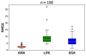
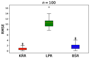
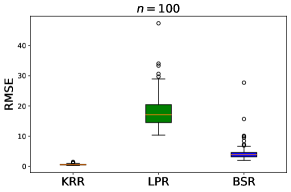
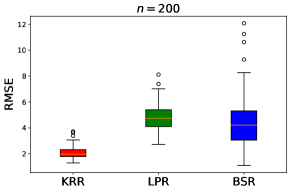
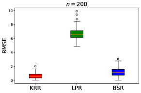
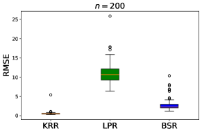
Figure 1: RMSE with $b=1$. DGP 1: left two panels, DGP 2: middle two panels, DGP 3: right two panels.

5.2 Bootstrap Hypothesis Testing

In this section, we investigate the empirical sizes and powers of the bootstrap hypothesis testing procedure proposed in Algorithm 1. Figures 2 reports the empirical rejection rates (ERR) for each DGP with $\alpha=1$, $\sigma=0.5,0.1,1.5$, and $b\in[-1,1]$. Each experiment is repeated 1000 times. It is straightforward to see that, when $b=0$, the rates are close to the nominal size, indicating the Type I error could be well controlled as stated in Theorem 5. When considering any value of $|b|$ greater than $0$, it can be observed that the EERs increase as the sample size $n$ grows larger. Given a sample size $n$, an increase in $|b|$ leads to an increase in the ERR. It is also easy to observe that as the signal-to-noise ratio increases (i.e., $\sigma$ decreases), the EER increases regardless of the sample size and $b$.

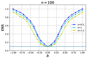
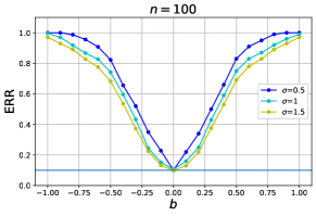
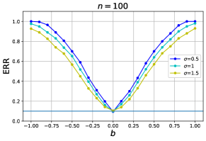
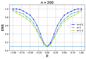
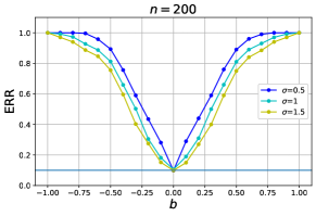
Figure 2: Empirical rejection rates with $\alpha=0.1$. DGP 1: left two panels, DGP 2: middle two panels, DGP 3: right two panels.

6 Empirical Application

In this section, we apply the proposed method to the ozone concentration dataset. This dataset contains measurements of air quality in 111 days from May to September 1973 in New York, which is available in the R package “ElemStatLearn”. The response variable, denoted as $y$, represents the ozone concentration. The dataset includes three predictors: solar radiation ($X_{1}$), wind speed ($X_{2}$), and temperature ($X_{3}$). For our analysis, we standardize all the independent variables to the interval $[0,1]$ using the transformation $x\to x/x_{\max}$.

We start with a KRR analysis using three dependent variables $(r=3)$ and up to three-way interactions $(q=3)$. A series of hypothesis testing is conducted for model selection. The bootstrap p-values for testing derivatives with first- and second-order are all less than 0.05 (almost zero). First, it reveals that all the covariates are highly informative. This finding aligns with visual inspections of the scatter plots in Figure 3. Furthermore, the p-values for testing second-order derivatives also suggest the presence of significant interactions for $(X_{1},X_{2})$, $(X_{2},X_{3})$, and $(X_{1},X_{3})$. Similar findings can be observed in the heat maps in Figure 4. For example, in the first subplot of Figure 4, when $(X_{1},X_{2})$ is close to $(1,0)$ (bottom right), the response shows a noticeably larger value than those in other locations. This observation suggests that there is a synergistic effect between $X_{1}$ and $X_{2}$ in influencing $y$. We next examine the presence of three-way interactions between the covariates, and the corresponding p-value is 0.72, indicating substantially less statistical significance compared to the lower-order counterparts. We also plot the histograms of $B=2000$ bootstrap samples for each test statistic in Figure 5. The plots suggest that the bootstrap procedure can be used to approximate the limiting distribution of the test statistic even though it is skewed.

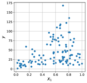
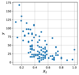
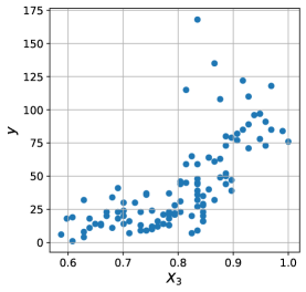
Figure 3: Scatter plots for response against predictors

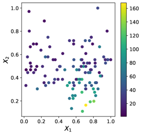
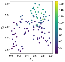
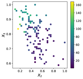
Figure 4: Heat maps for predictor pairs

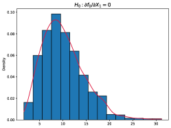
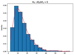
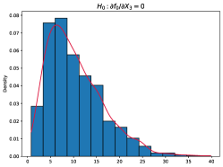
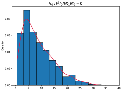
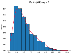
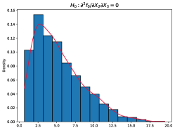
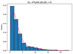
Figure 5: Histograms of bootstrap samples

Using the above exploration, our method suggests a model including $X_{1},X_{2},X_{3}$, and all their interactions up to order two $(q=2)$. This particular model structure illustrates how our method can inform otherwise challenging model-building decisions. We compare our models (KRR with $q=1,2,3$) with the following three single index models (SIM) appeared in Wang and Ke (2009): (a) $y=g(\theta_{1}X_{1}+\theta_{2}X_{2}+\sqrt{1-\theta_{1}^{2}-\theta_{2}^{2}}X_{3})+\epsilon$, (b) $y=\theta_{1}X_{1}+g(\theta_{2}X_{2}+\sqrt{1-\theta_{2}^{2}}X_{3})+\epsilon$, and (c) $y=g_{1}(X_{1})+g_{2}(\theta_{2}X_{2}+\sqrt{1-\theta_{2}^{2}}X_{3})+\epsilon$. For this purpose, we randomly divide the entire dataset by an $80/20$ split for training and prediction, and the averaged prediction errors and standard deviations are calculated based on 100 replications. The results are summarized in Table 1. It shows that the additive model (KRR 1) has the worst performance, while the selected model (KRR 2) performs best, suggesting high predictive power while maintaining model parsimony.

Table 1: Prediction errors

Our Models	Error	Models in Wang and Ke (2009)	Error [t]
KRR 1	22.05 (4.68)	SIM (a)	21.68 (4.04)
KRR 2	17.88 (3.69)	SIM (b)	20.57 (3.92)
KRR 3	18.96 (3.77)	SIM (c)	19.82 (3.72) [b]

Note: KRR $1,2,3$ stand for KRR with $q=1,2,3$.

7 Conclusion

In this paper, we propose a plug-in KRR estimator for estimating derivatives of the underlying regression function in SS-ANOVA models. The proposed estimator can be easily calculated and enjoys favorable theoretical properties. We first establish $L_{\infty}$ and $L_{2}$ convergence rates of the proposed estimator under general random designs. Additionally, we also show that the $L_{2}$ convergence rate is sharp under certain order conditions on the derivatives. Motivated by the wide range of real-world applications, we introduce a hypothesis testing procedure to examine a global zero partial derivative structure. To address the difficulty in estimating the critical value of the test, we also develop an associated bootstrap algorithm to construct the rejection region and calculate the p-value.

There are several interesting next directions building on our approach. First, it is interesting to develop model selection and interaction selection methods with a controlled rate such as the false discovery rate, particularly in situations with high-dimensional covariates. In addition, a natural step is to derive the weak convergence of the process $\mathbf{x}\to\partial^{\bm{\beta}}\widehat{f}(\mathbf{x})$, which enables the construction of simultaneous confidence corridors. Finally, there may be a need to extend the minimax lower bound established in Theorem 3 to encompass other $\bm{\beta}$ that hold practical significance.

References

- Atalla et al. (2018) Atalla, T. N., A. A. Gasim, and L. C. Hunt (2018). Gasoline demand, pricing policy, and social welfare in saudi arabia: A quantitative analysis. Energy policy 114, 123–133.
- Banerjee et al. (2003) Banerjee, S., A. E. Gelfand, and C. Sirmans (2003). Directional rates of change under spatial process models. Journal of the American Statistical Association 98(464), 946–954.
- Charnes et al. (1985) Charnes, A., W. W. Cooper, B. Golany, L. Seiford, and J. Stutz (1985). Foundations of data envelopment analysis for pareto-koopmans efficient empirical production functions. Journal of Econometrics 30(1-2), 91–107.
- Chen et al. (2019) Chen, J., S. E. McIlroy, A. Archana, D. M. Baker, and G. Panagiotou (2019). A pollution gradient contributes to the taxonomic, functional, and resistome diversity of microbial communities in marine sediments. Microbiome 7, 1–12.
- Cheng and Shang (2015) Cheng, G. and Z. Shang (2015). Joint asymptotics for semi-nonparametric regression models with partially linear structure. Annals of Statistics 43(3), 1351–1390.
- Chernozhukov et al. (2016) Chernozhukov, V., D. Chetverikov, and K. Kato (2016). Empirical and multiplier bootstraps for suprema of empirical processes of increasing complexity, and related gaussian couplings. Stochastic Processes and their Applications 126(12), 3632–3651.
- Cristianini and Shawe-Taylor (2000) Cristianini, N. and J. Shawe-Taylor (2000). An Introduction to Support Vector Machines and Other Kernel-based Learning Methods. Cambridge University press.
- Dai (2022) Dai, X. (2022). Nonparametric estimation via mixed gradients. arXiv preprint arXiv:2209.07672.
- Dai and Chien (2017) Dai, X. and P. Chien (2017). Minimax optimal rates of estimation in functional anova models with derivatives. arXiv preprint arXiv:1706.00850.
- Deaton (1986) Deaton, A. (1986). Demand analysis. Volume 3 of Handbook of Econometrics, pp. 1767–1839. Elsevier.
- Dong et al. (2017) Dong, X., S. Chen, and S. Pan (2017). Learning to prune deep neural networks via layer-wise optimal brain surgeon. In Advances in Neural Information Processing Systems, Volume 30.
- Exterkate et al. (2016) Exterkate, P., P. J. Groenen, C. Heij, and D. van Dijk (2016). Nonlinear forecasting with many predictors using kernel ridge regression. International Journal of Forecasting 32(3), 736–753.
- Gao et al. (2001) Gao, F., G. Wahba, R. Klein, and B. Klein (2001). Smoothing spline anova for multivariate bernoulli observations with application to ophthalmology data. Journal of the American Statistical Association 96(453), 127–160.
- Gu (2013) Gu, C. (2013). Smoothing Spline ANOVA Models. Springer New York, NY.
- Hastie et al. (2009) Hastie, T., R. Tibshirani, and J. Friedman (2009). The Elements of Statistical Learning: Data mining, Inference, and Prediction. Springer Science & Business Media.
- Hastie (2017) Hastie, T. J. (2017). Generalized additive models. In Statistical models in S, pp. 249–307. Routledge.
- Hu and Zastawniak (2020) Hu, W. and T. Zastawniak (2020). Pricing high-dimensional american options by kernel ridge regression. Quantitative Finance 20(5), 851–865.
- Huang (1998) Huang, J. (1998). Projection estimation in multiple regression with application to functional anova models. Annals of Statistics 26(1), 242–272.
- Kumar and Aravind (2008) Kumar, B. V. and R. Aravind (2008). Face hallucination using olpp and kernel ridge regression. In 2008 15th IEEE International Conference on Image Processing, pp. 353–356. IEEE.
- Li et al. (2021) Li, M., Z. Liu, C.-H. Yu, and M. Vannucci (2021). Semiparametric Bayesian inference for local extrema of functions in the presence of noise. arXiv preprint arXiv:2103.10606.
- Lian (2022) Lian, H. (2022). Distributed learning of conditional quantiles in the reproducing kernel hilbert space. In Advances in Neural Information Processing Systems, Volume 35, pp. 11686–11696.
- Lin (2000) Lin, Y. (2000). Tensor product space anova models. Annals of Statistics 28(3), 734–755.
- Lin and Zhang (2006) Lin, Y. and H. H. Zhang (2006). Component selection and smoothing in multivariate nonparametric regression. Annals of Statistics 34(5), 2272 – 2297.
- Liu et al. (2019) Liu, M., Z. Shang, and G. Cheng (2019). Sharp theoretical analysis for nonparametric testing under random projection. In Conference on Learning Theory, Volume 99, pp. 2175–2209.
- Liu et al. (2020) Liu, M., Z. Shang, and G. Cheng (2020). Nonparametric distributed learning under general designs. Electronic Journal of Statistics 14(2), 3070 – 3102.
- Liu and De Brabanter (2018) Liu, Y. and K. De Brabanter (2018). Derivative estimation in random design. In Advances in Neural Information Processing Systems, Volume 31.
- Liu and De Brabanter (2020) Liu, Y. and K. De Brabanter (2020). Smoothed nonparametric derivative estimation using weighted difference quotients. Journal of Machine Learning Research 21(1), 2438–2482.
- Liu and Li (2023) Liu, Z. and M. Li (2023). On the estimation of derivatives using plug-in kernel ridge regression estimators. Journal of Machine Learning Research. To appear, arXiv preprint arXiv:2006.01350.
- Luo et al. (1998) Luo, Z., G. Wahba, and D. R. Johnson (1998). Spatial–temporal analysis of temperature using smoothing spline anova. Journal of Climate 11(1), 18–28.
- Sang et al. (2022) Sang, P., Z. Shang, and P. Du (2022). Statistical inference for functional linear quantile regression. arXiv preprint arXiv:2202.11747.
- Shang (2010) Shang, Z. (2010). Convergence rate and Bahadur type representation of general smoothing spline M-estimates. Electronic Journal of Statistics 4, 1411 – 1442.
- Shang and Cheng (2013) Shang, Z. and G. Cheng (2013). Local and global asymptotic inference in smoothing spline models. Annals of Statistics 41(5), 2608–2638.
- Shang and Cheng (2015) Shang, Z. and G. Cheng (2015). Nonparametric inference in generalized functional linear models. Annals of Statistics 43(4), 1742 – 1773.
- Shephard (2015) Shephard, R. W. (2015). Theory of Cost and Production Functions. Princeton University Press.
- Song et al. (2006) Song, P. X.-K., X. Gao, R. Liu, and W. Le (2006). Nonparametric inference for local extrema with application to oligonucleotide microarray data in yeast genome. Biometrics 62(2), 545–554.
- Steinwart et al. (2009) Steinwart, I., D. R. Hush, C. Scovel, et al. (2009). Optimal rates for regularized least squares regression. In Conference on Learning Theory, pp. 79–93.
- Stone (1982) Stone, C. J. (1982). Optimal global rates of convergence for nonparametric regression. Annals of Statistics 10(4), 1040–1053.
- Sun et al. (2018) Sun, X., P. Du, X. Wang, and P. Ma (2018). Optimal penalized function-on-function regression under a reproducing kernel hilbert space framework. Journal of the American Statistical Association 113(524), 1601–1611.
- Touzani and Busby (2013) Touzani, S. and D. Busby (2013). Smoothing spline analysis of variance approach for global sensitivity analysis of computer codes. Reliability Engineering & System Safety 112, 67–81.
- Wahba (2003) Wahba, G. (2003). An introduction to smoothing spline anova models in rkhs, with examples in geographical data, medicine, atmospheric sciences and machine learning. IFAC Proceedings Volumes 36(16), 531–536. 13th IFAC Symposium on System Identification (SYSID 2003), Rotterdam, The Netherlands, 27-29 August, 2003.
- Wahba and Luo (1996) Wahba, G. and Z. Luo (1996). Smoothing spline anova fits for very large, nearly regular data sets, with application to historical global climate data. Annals of Numerical Mathematics 4, 579–598.
- Wahba et al. (1995) Wahba, G., Y. Wang, C. Gu, R. Klein, and B. Klein (1995). Smoothing spline anova for exponential families, with application to the wisconsin epidemiological study of diabetic retinopathy: the 1994 neyman memorial lecture. Annals of Statistics 23(6), 1865–1895.
- Wang and Lin (2015) Wang, W. W. and L. Lin (2015). Derivative estimation based on difference sequence via locally weighted least squares regression. Journal of Machine Learning Research 16(1), 2617–2641.
- Wang (1998) Wang, Y. (1998). Smoothing spline models with correlated random errors. Journal of the American Statistical Association 93(441), 341–348.
- Wang and Ke (2009) Wang, Y. and C. Ke (2009). Smoothing spline semiparametric nonlinear regression models. Journal of Computational and Graphical Statistics 18(1), 165–183.
- Wang et al. (2022) Wang, Y., Y. Zhou, R. Li, and H. Lian (2022). Sparse high-dimensional semi-nonparametric quantile regression in a reproducing kernel hilbert space. Computational Statistics & Data Analysis 168, 107388.
- Wang et al. (2022) Wang, Z., H. Dong, P. Ma, and Y. Wang (2022). Estimation and model selection for nonparametric function-on-function regression. Journal of Computational and Graphical Statistics 31(3), 835–845.
- Woodall et al. (2004) Woodall, W. H., D. J. Spitzner, D. C. Montgomery, and S. Gupta (2004). Using control charts to monitor process and product quality profiles. Journal of Quality Technology 36(3), 309–320.
- Xia (1998) Xia, Y. (1998). Bias-corrected confidence bands in nonparametric regression. Journal of the Royal Statistical Society: Series B 60(4), 797–811.
- Yang et al. (2003) Yang, L., S. Sperlich, and W. Härdle (2003). Derivative estimation and testing in generalized additive models. Journal of Statistical Planning and Inference 115(2), 521–542.
- Yu et al. (2022) Yu, J., J. Shi, A. Liu, and Y. Wang (2022). Smoothing spline semiparametric density models. Journal of the American Statistical Association 117(537), 237–250.
- Yuan and Cai (2010) Yuan, M. and T. T. Cai (2010). A reproducing kernel Hilbert space approach to functional linear regression. Annals of Statistics 38(6), 3412 – 3444.
- Zhang et al. (2016) Zhang, C., Y. Liu, and Y. Wu (2016). On quantile regression in reproducing kernel hilbert spaces with the data sparsity constraint. Journal of Machine Learning Research 17(1), 1374–1418.
- Zhang and Lin (2006) Zhang, H. H. and Y. Lin (2006). Component selection and smoothing for nonparametric regression in exponential families. Statistica Sinica 16(3), 1021–1041.
- Zhang et al. (2018) Zhang, J., H. Jin, Y. Wang, X. Sun, P. Ma, and W. Zhong (2018). Smoothing spline anova models and their applications in complex and massive datasets. In Y. K.-N. Truong and M. Sarfraz (Eds.), Topics in Splines and Applications, Chapter 4. Rijeka: IntechOpen.
- Zhang (2005) Zhang, T. (2005). Learning bounds for kernel regression using effective data dimensionality. Neural Computation 17(9), 2077–2098.
- Zhang et al. (2015) Zhang, Y., J. Duchi, and M. Wainwright (2015). Divide and conquer kernel ridge regression: A distributed algorithm with minimax optimal rates. Journal of Machine Learning Research 16(1), 3299–3340.
- Zhao et al. (2021) Zhao, S., R. Liu, and Z. Shang (2021). Statistical inference on panel data models: a kernel ridge regression method. Journal of Business & Economic Statistics 39(1), 325–337.