Semi-Supervised Semantic Segmentation via Marginal Contextual Information

Abstract

We present a novel confidence refinement scheme that enhances pseudo-labels in semi-supervised semantic segmentation. Unlike current leading methods, which filter pixels with low-confidence predictions in isolation, our approach leverages the spatial correlation of labels in segmentation maps by grouping neighboring pixels and considering their pseudo-labels collectively. With this contextual information, our method, named S4MC, increases the amount of unlabeled data used during training while maintaining the quality of the pseudo-labels, all with negligible computational overhead. Through extensive experiments on standard benchmarks, we demonstrate that S4MC outperforms existing state-of-the-art semi-supervised learning approaches, offering a promising solution for reducing the cost of acquiring dense annotations. For example, S4MC achieves a 1.29 mIoU improvement over the prior state-of-the-art method on PASCAL VOC 12 with 366 annotated images. The code to reproduce our experiments is available at https://s4mcontext.github.io/.

1 Introduction

Supervised learning has been the driving force behind advancements in modern computer vision, including classification Krizhevsky et al. (2012); Dai et al. (2021), object detection Girshick (2015); Zong et al. (2022), and segmentation Zagoruyko et al. (2016); Chen et al. (2018a); Li et al. (2022); Kirillov et al. (2023). However, it requires extensive amounts of labeled data, which can be costly and time-consuming to obtain. In many practical scenarios, there is no shortage of available data, but only a fraction can be labeled due to resource constraints. This challenge has led to the development of semi-supervised learning (SSL; Rasmus et al., 2015; Berthelot et al., 2019; Sohn et al., 2020a; Yang et al., 2022a), a methodology that leverages both labeled and unlabeled data for model training.

This paper focuses on applying SSL to semantic segmentation, which has applications in various areas such as perception for autonomous vehicles Bartolomei et al. (2020), mapping Van Etten et al. (2018) and agriculture Milioto et al. (2018). SSL is particularly appealing for segmentation tasks, as manual labeling can be prohibitively expensive.

A widely adopted approach for SSL is pseudo-labeling Lee (2013); Arazo et al. (2020). This technique dynamically assigns supervision targets to unlabeled data during training based on the model’s predictions. To generate a meaningful training signal, it is essential to adapt the predictions before integrating them into the learning process. Several techniques have been proposed, such as using a teacher network to generate supervision to a student network Hinton et al. (2015). The teacher network can be made more powerful during training by applying a moving average to the student network’s weights Tarvainen and Valpola (2017). Additionally, the teacher may undergo weaker augmentations than the student Berthelot et al. (2019), simplifying the teacher’s task.

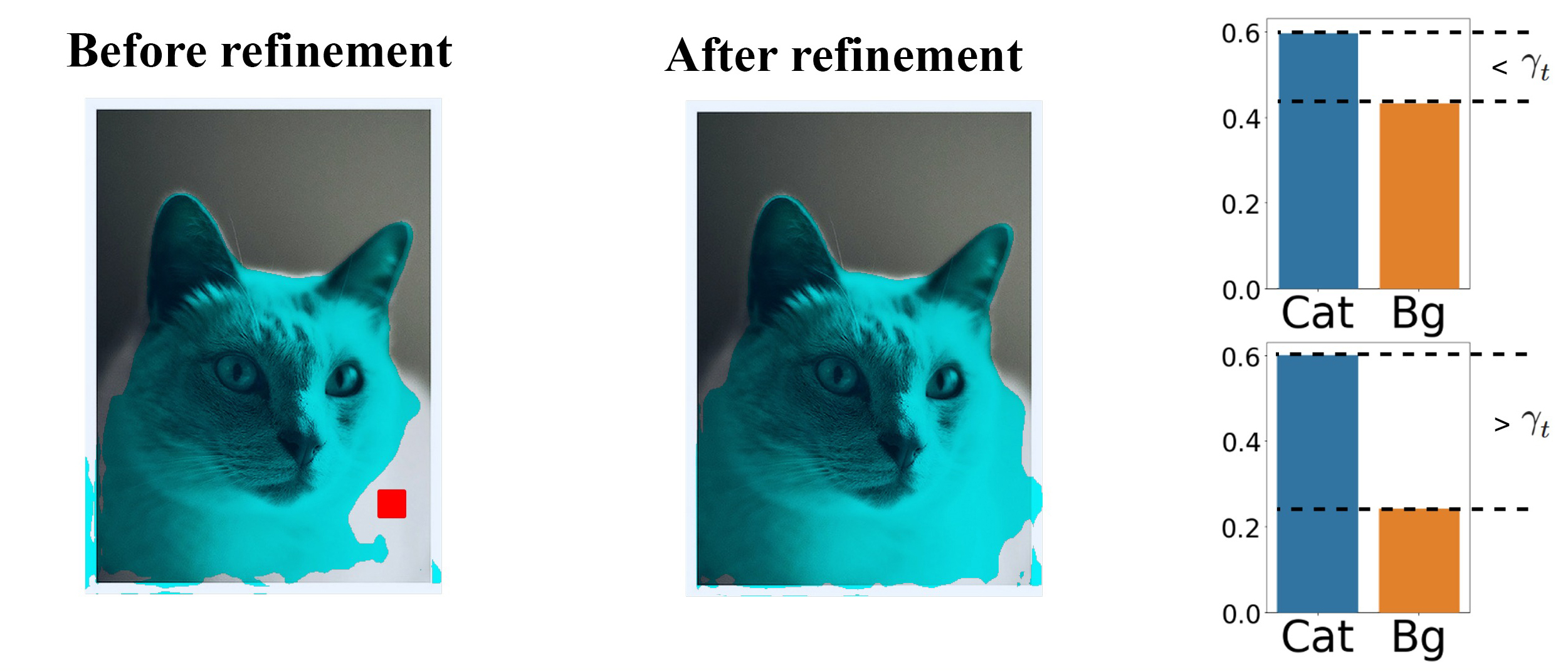
Figure 1: Confidence refinement. Left: pseudo-labels generated by the teacher network without refinement. Middle: pseudo-labels obtained from the same model after refinement with marginal contextual information. Right Top: predicted probabilities of the top two classes of the pixel highlighted by the red square before, and Bottom: after refinement. S4MC allows additional correct pseudo labels to propagate.

However, pseudo-labeling is intrinsically susceptible to confirmation bias, which tends to reinforce the model predictions instead of improving the student model. Mitigating confirmation bias becomes particularly important when dealing with erroneous predictions made by the teacher network.

Confidence-based filtering is a popular technique to address this issue  Sohn et al. (2020a). This approach assigns pseudo-labels only when the model’s confidence surpasses a specified threshold, thereby reducing the number of incorrect pseudo-labels. Though simple, this strategy was proven effective and inspired multiple improvements in semi-supervised classification Zhang et al. (2021); Rizve et al. (2021), segmentation Wang et al. (2022), and object detection in images Sohn et al. (2020b); Liu et al. (2021) and 3D scenes Zhao et al. (2020); Wang et al. (2021). However, the strict filtering of the supervision signal leads to extended training periods and, potentially, to overfitting when the labeled instances used are insufficient to represent the entire sample distribution. Lowering the threshold would allow for higher training volumes at the cost of reduced quality, further hindering the performance Sohn et al. (2020a).

In response to these challenges, we introduce a novel confidence refinement scheme for the teacher network predictions in segmentation tasks designed to increase the availability of pseudo-labels without sacrificing their accuracy. Drawing on the observation that labels in segmentation maps exhibit strong spatial correlation, we propose to group neighboring pixels and collectively consider their pseudo-labels. When considering pixels in spatial groups, we asses the event-union probability, which is the probability that at least one pixel belongs to a given class. We assign a pseudo-label if this probability is sufficiently larger than the event-union probability of any other class. By taking context into account, our approach Semi-Supervised Semantic Segmentation via Marginal Contextual Information (S4MC), enables a relaxed filtering criterion which increases the number of unlabeled pixels utilized for learning while maintaining high-quality labeling, as demonstrated in Fig. 1.

We evaluated S4MC on multiple semi-supervised segmentation benchmarks. S4MC achieves significant improvements in performance over previous state-of-the-art methods. In particular, we observed an increase of +1.29 mIoU on PASCAL VOC 12 Everingham et al. (2010) using 366 annotated images and an increase of +1.01 mIoU on Cityscapes Cordts et al. (2016) using only 186 annotated images. These findings highlight the effectiveness of S4MC in producing high-quality segmentation results with minimal labeled data.

2 Related Work

2.1 Semi-Supervised Learning

Pseudo-labeling Lee (2013) is a popular and effective technique in SSL, where labels are assigned to unlabeled data based on model predictions. To make the most of these labels during training, it is essential to refine them Laine and Aila (2016); Berthelot et al. (2019, 2020); Xie et al. (2020). One way to achieve this is through consistency regularization Laine and Aila (2016); Tarvainen and Valpola (2017); Miyato et al. (2018), which ensures consistent predictions between different views of the unlabeled data. Alternatively, a teacher model can be used to obtain pseudo-labels, which are then used to train a student model. To ensure that the pseudo-labels are helpful, the temperature of the prediction (soft pseudo-labels; Berthelot et al., 2019) can be increased, or the label can be assigned to samples with high confidence (hard pseudo-labels; Xie et al., 2020; Sohn et al., 2020a; Zhang et al., 2021). In this work, we follow the hard pseudo-label assignment approach and improve upon previous methods by proposing a confidence refinement scheme.

2.2 Semi-Supervised Semantic Segmentation

In semantic segmentation, most SSL methods rely on consistency regularization and developing augmentation strategies compatible with segmentation tasks French et al. (2020); Ke et al. (2020); Chen et al. (2021); Zhong et al. (2021); Xu et al. (2022). Given the uneven distribution of labels typically encountered in segmentation maps, techniques such as adaptive sampling, augmentation, and loss re-weighting are commonly employed Hu et al. (2021). Feature perturbations (FP) on unlabeled data Ouali et al. (2020); Zou et al. (2021); Liu et al. (2022b); Yang et al. (2023b) are also used to enhance consistency and the virtual adversarial training Liu et al. (2022b). Curriculum learning strategies that incrementally increase the proportion of data used over time are beneficial in exploiting more unlabeled data Yang et al. (2022b); Wang et al. (2022). A recent approach introduced by Wang et al. (2022) used unreliable predictions by employing contrastive loss with the least confident classes predicted by the model. Unimatch Yang et al. (2023b) combined SSL (Sohn et al., 2020a) with several self-supervision signals, i.e., two strong augmentations and one more with FP, obtained good results without complex losses or class-level heuristics. However, most existing works primarily focus on individual pixel label predictions. In contrast, we delve into the contextual information offered by spatial predictions on unlabeled data.

2.3 Contextual Information

Contextual information encompasses environmental cues that assist in interpreting and extracting meaningful insights from visual perception Toussaint (1978); Elliman and Lancaster (1990). Incorporating spatial context explicitly has been proven beneficial in segmentation tasks, for example, by encouraging smoothness like in the Conditional Random Fields method Chen et al. (2018a) and attention mechanisms Vaswani et al. (2017); Dosovitskiy et al. (2021); Wang et al. (2020). Combating dependence on context has shown to be helpful by Nekrasov et al. (2021). This work uses the context from neighboring pixel predictions to enhance pseudo-label propagation.

3 Method

This section describes the proposed method using the teacher–student paradigm. Adjustments from teacher–student consistency to weak–strong image-level consistency are described in Appendix C.

3.1 Overview

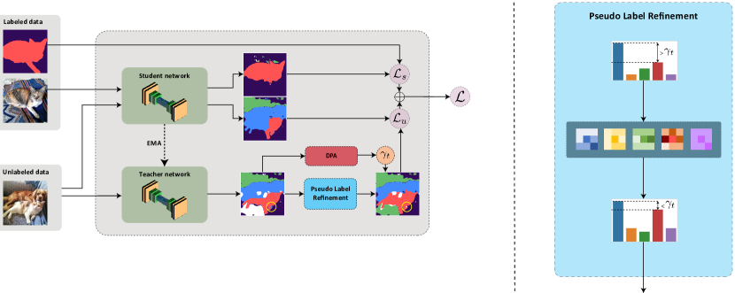
Figure 2: Left: S4MC employs a teacher-student paradigm for semi-supervised segmentation. Labeled images are used to supervise the student network directly; both teacher and student networks process unlabeled images. Predictions from the teacher network are refined and used to evaluate the margin value, which is then thresholded to produce pseudo-labels that guide the student network. The threshold, denoted as $\gamma_{t}$, is dynamically adjusted based on the teacher network’s predictions. Right: Our confidence refinement module exploits neighboring pixels to adjust per-class predictions, as detailed in Section 3.2.1. The class distribution of the pixel marked by the yellow circle on the left is changed. Before refinement, the margin surpasses the threshold and erroneously assigns the blue class (dog) as a pseudo-label. However, after refinement, the margin significantly reduces, thereby preventing the propagation of this error.

In semi-supervised semantic segmentation, we are given a labeled training set of images $\mathcal{D}_{\ell}=\left\{(\mathbf{x}_{i}^{\ell},\mathbf{y}_{i})\right\}_{i=1}^{N_{\ell}}$, and an unlabeled set $\mathcal{D}_{u}=\left\{\mathbf{x}_{i}^{u}\right\}_{i=1}^{N_{u}}$ sampled from the same distribution, i.e., $\quantity{\mathbf{x}_{i}^{\ell},\mathbf{x}_{i}^{u}}\sim D_{x}$. Here, $\mathbf{y}$ are 2D tensors of shape $H\times W$, assigning a semantic label to each pixel of $\mathbf{x}$. We aim to train a neural network $f_{\theta}$ to predict the semantic segmentation of unseen images sampled from $D_{x}$.

We follow a teacher–student approach Tarvainen and Valpola (2017) and train two networks $f_{\theta_{s}}$ and $f_{\theta_{t}}$ that share the same architecture but update their parameters separately. The student network $f_{\theta_{s}}$ is trained using supervision from the labeled samples and pseudo-labels created by the teacher’s predictions for unlabeled ones. The teacher model $f_{\theta_{t}}$ is updated as an exponential moving average (EMA) of the student weights. $f_{\theta_{s}}(\mathbf{x}_{i})$ and $f_{\theta_{t}}(\mathbf{x}_{i})$ denote the predictions of the student and teacher models for the $\mathbf{x}_{i}$ sample, respectively. At each training step, a batch of $\mathcal{B}_{\ell}$ and $\mathcal{B}_{u}$ images is sampled from $\mathcal{D}_{\ell}$ and $\mathcal{D}_{u}$, respectively. The optimization objective can be written as the following loss:

$$\mathcal{L} =\mathcal{L}_{s}+\lambda\mathcal{L}_{u}$$ (1)

$$\mathcal{L}_{s} =\frac{1}{M_{l}}\sum_{\mathbf{x}_{i}^{\ell},\mathbf{y}_{i}\in\mathcal{B}_{l}}\ell_{CE}(f_{\theta_{s}}(\mathbf{x}_{i}^{\ell}),\mathbf{y}_{i})$$ (2)

$$\mathcal{L}_{u} =\frac{1}{M_{u}}\sum_{\mathbf{x}_{i}^{u}\in\mathcal{B}_{u}}\ell_{CE}(f_{\theta_{s}}(\mathbf{x}_{i}^{u}),\hat{\mathbf{y}}_{i}),$$ (3)

where $\mathcal{L}_{s}$ and $\mathcal{L}_{u}$ are the losses over the labeled and unlabeled data correspondingly, $\lambda$ is a hyperparameter controlling their relative weight, and $\hat{\mathbf{y}}_{i}$ is the pseudo-label for the $i$-th unlabeled image. Not every pixel of $\mathbf{x}_{i}$ has a corresponding label or pseudo-label, and $M_{l}$ and $M_{u}$ denote the number of pixels with label and assigned pseudo-label in the image batch, respectively.

3.1.1 Pseudo-label Propagation

For a given image $\mathbf{x}_{i}$, we denote by $\mathbf{x}^{i}_{j,k}$ the pixel in the $j$-th row and $k$-th column. We adopt a thresholding-based criterion inspired by FixMatch Sohn et al. (2020a). By establishing a score, denoted as $\kappa$, which is based on the class distribution predicted by the teacher network, we assign a pseudo-label to a pixel if its score exceeds a threshold $\gamma_{t}$:

$$\hat{\mathbf{y}}^{i}_{j,k}=\begin{cases}\arg\max_{c}\{p_{c}(x^{i}_{j,k})\}&\text{if}\ \kappa(x^{i}_{j,k};\theta_{t})>\gamma_{t},\\ \text{ignore}&\text{otherwise},\end{cases},$$ (4)

where $p_{c}(x^{i}_{j,k})$ is the pixel probability of class $c$. A commonly used score is given by $\kappa(x^{i}_{j,k};\theta_{t})=\max_{c}\{p_{c}(x^{i}_{j,k})\}$. However, we found that using a pixel-wise margin, similar to scores proposed by Scheffer et al. (2001) and Shin et al. (2021), produces more stable results. This approach calculates the margin as the difference between the highest and the second-highest values of the probability vector:

$$\kappa_{\text{margin}}(x^{i}_{j,k})=\max_{c}\{p_{c}(x^{i}_{j,k})\}-\operatorname*{\mathrm{max2}}_{c}\{p_{c}(x^{i}_{j,k})\},$$ (5)

where $\mathrm{max2}$ denotes the vector’s second highest value.

3.1.2 Dynamic Partition Adjustment (DPA)

Following Wang et al. (2022), we use a decaying threshold $\gamma_{t}$. DPA replaces the fixed threshold with a quantile-based threshold that decreases with time. At each iteration, we set $\gamma_{t}$ as the $\alpha_{t}$-th quantile of $\kappa_{\text{margin}}$ over all pixels of all images in the batch. We use linearly decreasing $\alpha_{t}$:

$$\alpha_{t}=\alpha_{0}\cdot\quantity(1-\nicefrac{{t}}{{\mathrm{iterations}}}).$$ (6)

As the model predictions improve with each iteration, gradually lowering the threshold increases the number of propagated pseudo-labels without compromising their quality.

3.2 Marginal Contextual Information

Utilizing contextual information (Section 2.3), we look at surrounding predictions (predictions on neighboring pixels) to refine the semantic map at each pixel. We introduce the concept of “Marginal Contextual Information,” which involves integrating additional information to enhance predictions across all classes. At the same time, reliability-based pseudo-label methods focus on the dominant class only Sohn et al. (2020a); Wang et al. (2023). Section 3.2.1 describes our confidence refinement, followed by our thresholding strategy and a description of S4MC methodology.

3.2.1 Confidence Margin Refinement

We refine the predicted pseudo-label of each pixel by considering the predictions of its neighboring pixels. Given a pixel $x^{i}_{j,k}$ with a corresponding per-class prediction $p_{c}(x^{i}_{j,k})$, we examine neighboring pixels $x^{i}_{\ell,m}$ within an $N\times N$ pixel neighborhood surrounding it. We then calculate the probability that at least one of the two pixels belongs to class $c$:

$$\tilde{p}_{c}(x^{i}_{j,k})=p_{c}(x^{i}_{j,k})+p_{c}(x^{i}_{\ell,m})-p_{c}(x^{i}_{j,k},x^{i}_{\ell,m}),$$ (7)

where $p_{c}(x^{i}_{j,k},x^{i}_{\ell,m})$ denote the joint probability of both $x^{i}_{j,k}$ and $x^{i}_{\ell,m}$ belonging to the same class $c$.

While the model does not predict joint probabilities, it is reasonable to assume a non-negative correlation between the probabilities of neighboring pixels. This is largely due to the nature of segmentation maps, which are typically piecewise constant. Consequently, any information regarding the model’s prediction of neighboring pixels belonging to a specific class should not lead to a reduction in the posterior probability of the given pixel also falling into that class. The joint probability can thus be bounded from below by assuming independence: $p_{c}(x^{i}_{j,k},x^{i}_{\ell,m})\geqslant p_{c}(x^{i}_{j,k})\cdot p_{c}(x^{i}_{\ell,m})$. By substituting this into Eq. 7, we obtain an upper bound for the event union probability:

$$\tilde{p}_{c}(x^{i}_{j,k})\leq p_{c}(x^{i}_{j,k})+p_{c}(x^{i}_{\ell,m})-p_{c}(x^{i}_{j,k})\cdot p_{c}(x^{i}_{\ell,m}).$$ (8)

This formulation allows us to filter out confidence margins that do not exceed the threshold.

For each class $c$, we select the neighbor with the maximal information gain using Eq. 8:

$$\tilde{p}_{c}^{\mathbf{N}}(x^{i}_{j,k})=\max_{\ell,m}\tilde{p}_{c}(x^{i}_{j,k}).$$ (9)

Computing the event union over all classes employs neighboring predictions to amplify differences in ambiguous cases. Similarly, this prediction refinement prevents the creation of over-confident predictions not supported by additional spatial evidence and helps reduce confirmation bias. The refinement is visualized in Fig. 1. In our experiments, we used a neighborhood size of $3\times 3$. To determine whether the incorporation of contextual information could be enhanced with larger neighborhoods, we conducted an ablation study focusing on the neighborhood size and the neighbor selection criterion, as detailed in Table 4(a). For larger neighborhoods, we decrease the probability contribution of the neighboring pixels with a distance-dependent factor:

$$\tilde{p}_{c}(x^{i}_{j,k})=p_{c}(x^{i}_{j,k})+\beta_{\ell,m}\quantity[p_{c}(x^{i}_{\ell,m})-p_{c}(x^{i}_{j,k},x^{i}_{\ell,m})],$$ (10)

where $\beta_{\ell,m}=\exp(-\frac{1}{2}(\absolutevalue{\ell-j}+\absolutevalue{m-k}))$ is a spatial weighting function. Empirically, contextual information refinement affects mainly the most probable one or two classes. This aligns well with our choice to use the margin confidence (5).

Considering more than two events (more than one neighbor), one can use the formulation for three or four event-union. In practice, we calculate it iteratively, starting with two event-union defined by Eq. 10, using it as $p_{c}(x^{i}_{j,k})$, finding the next desired event using Eq. 9 with the remaining neighbors, and repeating the process.

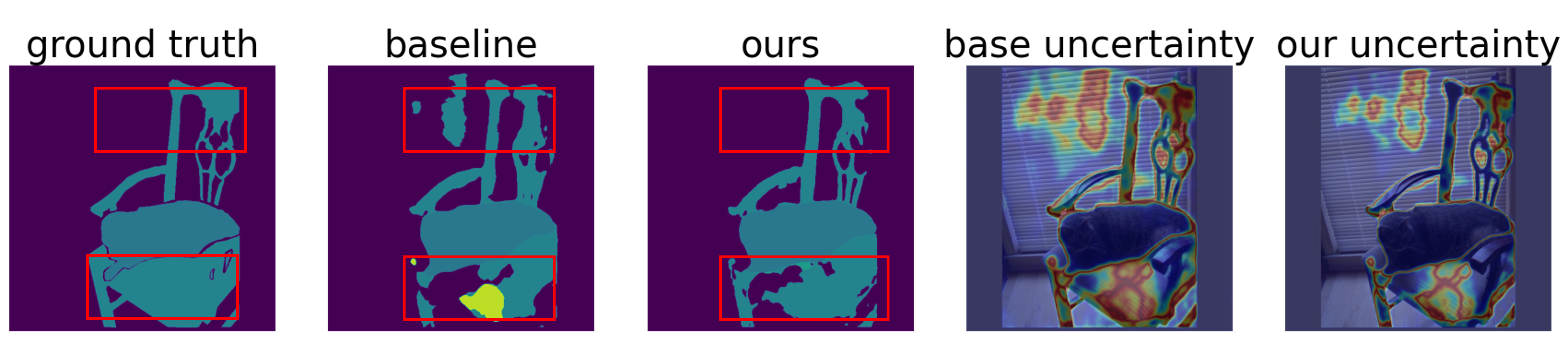
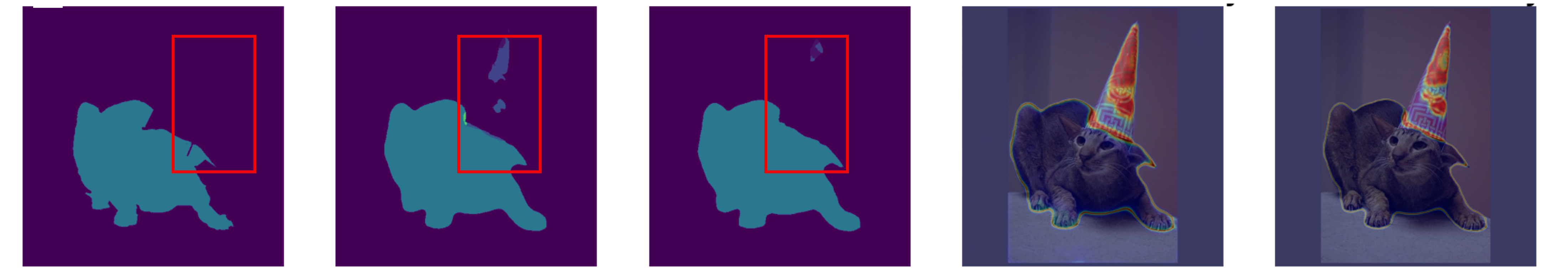
Figure 3: Qualitative results of S4MC. The outputs of two trained models and the annotated ground truth. The segmentation map predicted by S4MC (Ours) compared to the segmentation map using no refinement module (Baseline) and to the ground truth. Heat map represents the uncertainty of the model as $\kappa^{-1}$, showing a more confident prediction over certain areas, yielding to a smother segmentation maps (compared in the red boxes).

3.2.2 Threshold Setting

Setting a high threshold can prevent confirmation bias from the teacher model’s “beliefs” transferring to the student model. However, this comes at the expense of learning from fewer examples, potentially resulting in a less comprehensive model. For determining the DPA threshold, we use the teacher predictions pre-refinement $p_{c}(x^{i}_{j,k})$, but we filter values based on $\tilde{p}_{c}(x^{i}_{j,k})$. Consequently, more pixels pass the threshold that remains unaffected. We set $\alpha_{0}=0.4$, i.e., 60% of raw predictions pass the threshold at $t=0$, as this value demonstrated superior performance in our experiments. An ablation study for $\alpha_{0}$ is provided in Table 4(b).

3.3 Putting it All Together

We perform semi-supervised learning for semantic segmentation by pseudo-labeling pixels using their neighbors’ contextual information. Labeled images are only fed into the student model, producing the supervised loss (Eq. 2). Unlabeled images are fed into the student and teacher models. We sort the margin based $\kappa_{\text{margin}}$ (Eq. 5) values of teacher predictions and set $\gamma_{t}$ as described in Section 3.2.2. The per-class teacher predictions are refined using the weighted union event relaxation, as defined in Eq. 10. Pixels with higher margin values than $\gamma_{t}$ are assigned with pseudo-labels as described in Eq. 4, producing the unsupervised loss (Eq. 3). The entire pipeline is visualized in Fig. 2.

The impact of S4MC is demonstrated in Fig. 4, which compares the fraction of pixels that pass the threshold with and without refinement. Our method uses more unlabeled data during most of the training process (a), while the refinement ensures high-quality pseudo-labels (b). We further analyze the quality improvement by studying true positive (TP) and false positive (FP) rates, as shown in Fig. B.1 in the Appendix. Qualitative results are presented in Fig. 3, where one can see both the confidence heatmap and the pseudo-labels with and without the impact of S4MC.

4 Experiments

This section presents our experimental results. The setup for the different datasets and partition protocols is detailed in Section 4.1. Section 4.2 compares our method against existing approaches and Section 4.3 provides the ablation study. Further implementation details are given in Appendix G.

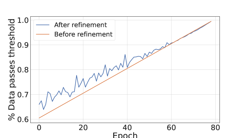
(a) Data fraction that passes the threshold. The baseline model has a fixed percentage, as it is based on DPA. Our method increases the number of pixels assigned pseudo-label, mostly in the early stage of the training when the model is under-confident.

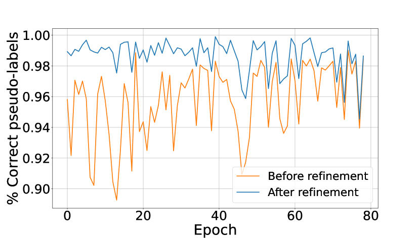
(b) Fraction of correct pseudo-labels the assigned pseudo-labels with the correct class divided by the total assigned pseudo-label. S4MC produces more quality pseudo-labels during the training process, most notably at the early stages.

Figure 4: Pseudo-label quantity and quality on PASCAL VOC 2012 Everingham et al. (2010) with 366 labeled images using our margin (5) confidence function.

Table 1: Comparison between our method and prior art on the PASCAL VOC 2012 val on different partition protocols. the caption describes the share of the training set used as labeled data and, in parentheses, the actual number of labeled images. Larger improvement can be observed for partitions of extremely low annotated data, where other methods suffer from starvation due to poor teacher generalization. * denotes reproduced results, $\psi$ denotes the use of UniMatch Yang et al. (2023a) without the use of feature perturbation.

Method	1/16 (92)	1/8 (183)	1/4 (366)	1/2 (732)	Full (1464)
CutMix-Seg French et al. (2020)	52.16	63.47	69.46	73.73	76.54
ReCo Liu et al. (2022a)	64.80	72.0	73.10	74.70	-
ST++ Yang et al. (2022b)	65.2	71.0	74.6	77.3	79.1
U2PL Wang et al. (2022)	67.98	69.15	73.66	76.16	79.49
PS-MT Liu et al. (2022b)	65.8	69.6	76.6	78.4	80.0
PCR Xu et al. (2022)	70.06	74.71	77.16	78.49	80.65
FixMatch* Yang et al. (2023a)	68.07	73.72	76.38	77.97	79.97
UniMatch* Yang et al. (2023a)	73.75	75.05	77.7	79.9	80.43
CutMix-Seg + S4MC	70.96	71.69	75.41	77.73	80.58
FixMatch + S4MC	73.13	74.72	77.27	79.07	79.6
$\text{UniMatch}^{\psi}$ + S4MC	74.72	75.21	79.09	80.12	81.56

4.1 Setup

Datasets

In our experiments, we use PASCAL VOC 2012 Everingham et al. (2010) and Cityscapes Cordts et al. (2016) datasets.

The PASCAL VOC dataset comprises 20 object classes (plus background). The dataset includes 2,913 annotated images, divided into a training set of 1,464 images and a validation set of 1,449 images. In addition, the dataset includes 9,118 coarsely annotated training images Hariharan et al. (2011), in which only a subset of the pixels are labeled. Following previous research, we conducted two sets of experiments. The ”classic“ setup uses only the original training set Wang et al. (2022); Zou et al. (2021), while the ”coarse“ setup uses all available data Wang et al. (2022); Chen et al. (2021); Hu et al. (2021).

The Cityscapes Cordts et al. (2016) dataset includes urban scenes from 50 different cities with 30 classes, of which only 19 are typically used for evaluation Chen et al. (2018a, b). Similarly to PASCAL, in addition to 2,975 training and 500 validation images, the dataset includes 19,998 coarsely annotated images, which we do not use in our experiment.

Implementation details

We implement S4MC on top of two framework variants: teacher-student Tarvainen and Valpola (2017); French et al. (2020) and consistency optimization Sohn et al. (2020a); Yang et al. (2023b). Both use DeepLabv3+ Chen et al. (2018b) with a Imagenet-pre-trained Russakovsky et al. (2015) ResNet-101 He et al. (2016). For the teacher–student setup, the teacher parameters $\theta_{t}$ are updated via an exponential moving average (EMA) of the student parameters (Tarvainen and Valpola, 2017): $\theta^{\eta}_{t}=\tau\theta^{\eta-1}_{t}+(1-\tau)\theta^{\eta}_{s},$ where $0\leq\tau\leq 1$ defines how close the teacher is to the student and $\eta$ denotes the training iteration. We used $\tau=0.99$. For the consistency paradigm, the teaching branch uses weak augmentations and the student branch uses strong ones. Additional details are provided in Appendix G.

Table 2: Comparison between our method and prior art on the ’coarse’ PASCAL VOC 2012 val dataset under different partition protocols, using additional unlabeled data from Hariharan et al. (2011). We included the number of labeled images in parentheses for each partition ratio. As in Table 1, larger improvements are observed for partitions with less annotated data. * denotes reproduced results, $\psi$ denotes the use of UniMatch Yang et al. (2023a) without the use of feature perturbation.

Method	1/16 (662)	1/8 (1323)	1/4 (2646)	1/2 (5291)
CutMix-Seg French et al. (2020)	71.66	75.51	77.33	78.21
AEL Hu et al. (2021)	77.20	77.57	78.06	80.29
PS-MT Liu et al. (2022b)	75.5	78.2	78.7	-
U2PL Wang et al. (2022)	77.21	79.01	79.3	80.50
PCR Xu et al. (2022)	78.6	80.71	80.78	80.91
FixMatch* Yang et al. (2023a)	74.35	76.33	76.87	77.46
UniMatch* Yang et al. (2023a)	76.6	77.0	77.32	77.9
S4MC + CutMix-Seg (Ours)	78.49	79.67	79.85	81.11
FixMatch + S4MC	75.19	76.56	77.11	78.07
$\text{UniMatch}^{\psi}$ + S4MC	76.95	77.54	77.62	78.08

Table 3: Comparison between our method and prior art on the Cityscapes val dataset under different partition protocols. Labeled and unlabeled images are selected from the Cityscapes training dataset. For each partition protocol, the caption gives the share of the training set used as labeled data, in parentheses, the number of labeled images. * denotes reproduced results, $\psi$ denotes the use of UniMatch Yang et al. (2023a) without the use of feature perturbation.

Method	1/16 (186)	1/8 (372)	1/4 (744)	1/2 (1488)
CutMix-Seg French et al. (2020)	69.03	72.06	74.20	78.15
AEL Hu et al. (2021)	74.45	75.55	77.48	79.01
U2PL Wang et al. (2022)	70.30	74.37	76.47	79.05
PS-MT Liu et al. (2022b)	-	76.89	77.6	79.09
PCR Xu et al. (2022)	73.41	76.31	78.4	79.11
FixMatch* Yang et al. (2023a)	74.17	76.2	77.14	78.43
UniMatch* Yang et al. (2023a)	75.99	77.55	78.54	79.22
CutMix-Seg + S4MC	75.03	77.02	78.78	78.86
FixMatch + S4MC	75.2	77.61	79.04	79.74
$\text{UniMatch}^{\psi}$ + S4MC	77.0	77.78	79.52	79.76

Evaluation

We compare S4MC with state-of-the-art methods and baselines under the common partition protocols – using $1/2$, $1/4$, $1/8$, and $1/16$ of the training set as labeled data. For the ’classic’ setting of the PASCAL experiment, we additionally compare using all the finely annotated images. We follow standard protocols and use mean Intersection over Union (mIoU) as our evaluation metric. We use the data split published by Wang et al. (2022) when available to ensure a fair comparison. We use PASCAL VOC 2012 val with $1/4$ partition for the ablation studies.

4.2 Results

PASCAL VOC 2012.

Table 1 compares our method with state-of-the-art baselines on the PASCAL VOC 2012 dataset. While Table 2 shows the comparison results on the PASCAL VOC 2012 dataset with additional coarsely annotated data from SBD Hariharan et al. (2011). In both setups, S4MC outperforms all the compared methods in standard partition protocols, both when using labels only for the original PASCAL VOC 12 dataset and when using SBD annotations as well. Qualitative results are shown in Fig. 3. As can be seen our refinement procedure aids in both adding falsely filtered pseudo-labels as well as removing erroneous ones.

Cityscapes.

Table 3 presents the comparison results on the Cityscapes val dataset. Table 3 compares our method with other state-of-the-art methods on the Cityscapes Cordts et al. (2016) dataset under various partition protocols. S4MC outperforms the compared methods in most partitions, except for the $1/2$ setting, and combined with the FixMatch scheme, S4MC outperforms compared approaches across all partitions.

Contextual information at inference.

Given that our margin refinement scheme operates through prediction adjustments, we explored whether it could be employed at inference time to enhance performance. The results reveal a negligible improvement in the DeepLab-V3-plus model, from an 85.7 mIOU to 85.71. This underlines that the performance advantage of S4MC primarily derives from the adjusted margin, as the most confident class is rarely swapped. A heatmap of the prediction over several samples is presented in Fig. 3 and Fig. H.1.

4.3 Ablation Study

We ablate different components of our method using the CutMix-Seg framework variant and evaluated using the Pascal VOC 12 dataset with a partition protocol of 1/4 labeled images.

Neighborhood size and neighbor selection criterion.

Our prediction refinement scheme employs event-union probability with neighboring pixels, which depends on the chosen neighbor to pair with the current pixel. To assess this, we tested varying neighborhood sizes ($N=3,5,7$) and criteria for selecting the neighboring pixel: (a) random, (b) maximal class probability, (c) minimal class probability, and (d) two neighbors, as described in Section 3.2.1. We also compare with $1\times 1$ neighborhood, which corresponds to not using S4MC at all. As shown in Table 4(a), a small $3\times 3$ neighborhood with one neighboring pixel of the highest class probability proved most efficient in our experiments.

Table 4: The effect of neighborhood size and neighbor selection criterion.

(a) Neighborhood choice.

Selection criterion	Neighborhood size $\mathbf{N}$
	$\mathbf{1\times 1}$	$\mathbf{3\times 3}$	$\mathbf{5\times 5}$	$\mathbf{7\times 7}$
Random neighbor	69.46	73.25	71.1	70.41
Max neighbor		75.41	75.18	74.89
Min neighbor		74.54	74.11	70.28
Two max neighbors		74.14	75.15	74.36

(b) $\alpha_{0}$ in Eq. 6, which controls the initial proportion of confidence pixels

20%	30%	40%	50%	60%
74.45	73.85	75.41	74.56	74.31

We also examine the contribution of the proposed pseudo-label refinement (PLR) as well as DPA. Results in Table 5 show that the PLR helps improve the mask mIoU by 1.09%, while DPA alone harms the performance. This indicates that PLR helps semi-supervised learning mainly because it enforces more spatial dependence on the pseudo-labels.

Table 5: Ablation study on the different components of S4MC on top of FixMatch. PLR is the pseudo-label refinement module and DPA is dynamic partition adjustment.

PLR	DPA	1/4
		76.8
✓		76.2
	✓	77.89
✓	✓	78.07

Threshold parameter tuning

As outlined in Section 3.1.2, we utilize a dynamic threshold that depends on an initial value, $\alpha_{0}$. In Table 4(b), we examine the effect of different initial quantiles to establish this threshold. A smaller $\alpha_{0}$ would propagate too many errors, leading to significant confirmation bias. In contrast, a larger $\alpha_{0}$ would mask most of the data, resulting in insufficient label propagation, rendering the semi-supervised learning process lengthy and inefficient. We found that an $\alpha_{0}$ of 40% yields the best performance.

5 Conclusion

In this paper, we introduce S4MC, a novel approach for incorporating spatial contextual information in semi-supervised segmentation. This strategy refines confidence levels and enables us to leverage more unlabeled data. S4MC outperforms existing approaches and achieves state-of-the-art results on multiple popular benchmarks under various data partition protocols, such as Cityscapes and Pascal VOC 12. Despite its effectiveness in lowering the annotation requirement, there are several limitations to using S4MC. First, its reliance on event-union relaxation is applicable only in cases involving spatial coherency. As a result, using our framework for other dense prediction tasks would require an examination of this relaxation’s applicability. Furthermore, our method uses a fixed-shape neighborhood without considering the object’s structure. It would be interesting to investigate the use of segmented regions to define new neighborhoods; this is a future direction we plan to explore.

Appendix A Limitations and Potential Negative Social Impacts

Limitations.

The constraint imposed by the spatial coherence assumption also restricts the applicability of this work to dense prediction tasks. Improving pseudo-labels’ quality for overarching tasks such as classification might necessitate reliance on data distribution and the exploitation of inter-sample relationships. We are currently exploring this avenue of research.

Societal impact.

Similar to most semi-supervised models, we utilize a small subset of annotated data, which can potentially introduce biases from the data into the model. Further, our PLR module assumes spatial coherence. While that holds for natural images, it may yield adverse effects in other domains, such as medical imaging. It is important to consider these potential impacts before choosing to use our proposed method.

Appendix B Pseudo-labels quality analysis

The quality improvement and the quantity increase of pseudo-labels are shown in Fig. 4. Further analysis of the quality improvement of our method is demonstrated in Fig. B.1 by separating the true positive and false positive.

Within the initial phase of the learning process, the enhancement in the quality of pseudo-labels can be primarily attributed to the advancement in true positive labels. In our method, the refinement not only facilitates the inclusion of a larger number of pixels surpassing the threshold but also ensures that a significant majority of these pixels are of high quality.

As the learning process progresses, most improvements are obtained from a decrease in false positives pseudo-labels. This analysis shows that our method effectively minimizes the occurrence of incorrect pseudo-labeled, particularly when the threshold is set to a lower value. In other words, our method reduces confirmation bias from decaying the threshold as the learning process progresses.

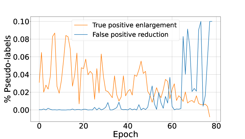
Figure B.1: Quality of pseudo-labels, on PASCAL VOC 2012 Everingham et al. (2010) over training iterations. Fig. 4 separated to True positive and False positive analysis. True positive are the bigger part of improvement at the early stage of the training process, while reduction of false positive is the main contribution late in the training process

Appendix C weak–strong consistency

To adjust the method to image level consistency framework Sohn et al. (2020a); Zhang et al. (2021); Wang et al. (2023), we need to re-define the supervision branch. Recall that within the teacher-student framework, we denote $f_{\theta_{s}}(\mathbf{x}_{i})$ and $f_{\theta_{t}}(\mathbf{x}_{i})$ as the predictions made by the student and teacher models for input $\mathbf{x}_{i}$, where the teacher serves as the source for generating confidence-based pseudo-labels. In the context of image-level consistency, both branches differ by augmented versions $\mathbf{x}^{w}_{i}$, $\mathbf{x}^{s}_{i}$ and share identical weights $f_{\theta}$. Here, $\mathbf{x}^{w}_{i}$ and $\mathbf{x}^{s}_{i}$ represent the weak and strong augmented renditions of the input $\mathbf{x}_{i}$, respectively. Following the aforementioned framework, it is the branch associated with weak augmentation that generates the pseudo-labels.

Appendix D Ablation studies

D.1 Confidence function alternatives

In this paper, we introduce a confidence function to determine pseudo-label propagation. We introduced $\kappa_{\text{margin}}(x_{i,j})$ and mentioned other alternatives have been examined.

Here, we define several options for the confidence function.

The simplest option is to look at the probability of the dominant class,

$$\kappa_{\text{max}}(x^{i}_{j,k})=\max_{c}{p_{c}(x^{i}_{j,k})},$$ (D.1)

which is commonly used to generate pseudo-labels.

The second alternative is negative entropy, defined as

$$\kappa_{\text{ent}}(x^{i}_{j,k})=\sum_{c\in C}p_{c}(x^{i}_{j,k})\log(p^{c}_{i,j}).$$ (D.2)

Note that this is indeed a confidence function since high entropy corresponds to high uncertainty, and low entropy corresponds to high confidence.

The third option is for us to define the margin function Scheffer et al. (2001); Shin et al. (2021) as the difference between the first and second maximal values of the probability vector and also described in the main paper:

$$\kappa_{\text{margin}}(x_{i,j})=\max_{c}(p_{c}(x^{i}_{j,k}))-\mathrm{max2}_{c}(p_{c}(x^{i}_{j,k})),$$ (D.3)

where $\mathrm{max2}$ denotes the vector’s second maximum value. All alternatives are compared in Table D.1.

Table D.1: Ablation study on the confidence function $\kappa$, over Pascal VOC 12 with partition protocols

Function	1/4 (366)	1/2 (732)	Full (1464)
$\kappa_{\text{max}}$	74.29	76.16	79.49
$\kappa_{\text{ent}}$	75.18	77.55	79.89
$\kappa_{\text{margin}}$	75.41	77.73	80.58

Table D.1 studies the impact of different confidence functions on pseudo-label refinement. We found that using a margin to describe confidence is a suitable way when there is a contradiction in smooth regions.

D.2 Decomposition and analysis of Unimatch

Unimatch Yang et al. (2023b) investigating the consistency and suggest to use FixMatch Sohn et al. (2020a) and a strong baseline for semi-supervised semantic segmentation. Moreover, they provide analysis that shows that combining 3 students for each supervision signal, one feature level augmentation, feature perturbation, denoted by FP, and two strong augmentations, denoted by S1 and S2. Fusing Unimatch and our method did not provide significant improvements, and we examined the contribution of different components of Unimatch. We measure the pixel-agreement as described in Eq. 10 and showed that the feature perturbation branch has the same effect on pixel-agreement as S4MC. Fig. 1(b) present the distribution of agreement using FixMatch (S1), DusPerb (S1,S2), Unimatch (S1, S2, FP) and S4MC (S1, S2).

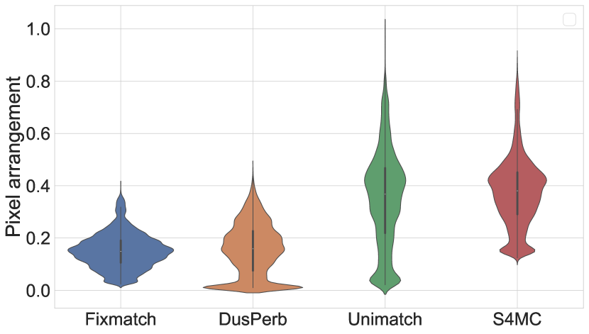
(a) The spatial agreement as we define in in 10 compared between different variations of Unimatch and S4MC, on PASCAL VOC 12 dataset.

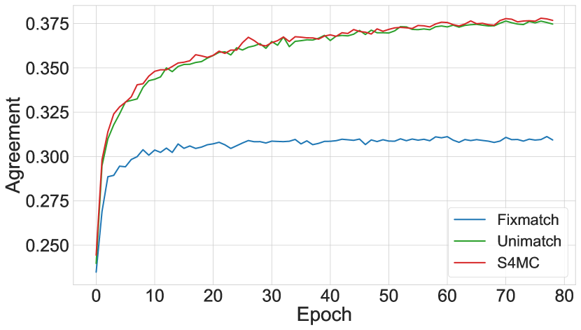
(b) The spatial agreement, compared between different variations of Unimatch Yang et al. (2023b) and S4MC, on PASCAL over time.

Appendix E Computational cost

Let us denote the image size by $H\times W$ and the number of classes by C.

First, the predicted map of dimension $H\times W\times C$ is stacked with the padded-shifted versions, creating a tensor of shape [n,H,W,C]. K top neighbors are picked via top-k operation and calculate the union event as presented in Eq. 10. (The pseudo label refinement pytorch-like pseudo-code can be obtained in Algorithm 1 for $N=4$ and $k$ max neighbors.)

The overall space (memory) complexity of the calculation is $O(n\times H\times W\times C)$, which is negligible considering all parameters and gradients of the model. Time complexity adds 3 tensor operations (stack, topk, and multiplication) over the $H\times W\times C$ tensor, where the multiplication operates k times, which means $O(k\times H\times W\times C)$. This is again negligible for any reasonable number of classes compared to tens of convolutional layers with hundreds of channels.

To verify that, we conducted a training time analysis comparing FixMatch and FixMatch + S4MC over PASCAL with 366 labeled examples, using distributed training with 8 Nvidia RTX 3090 GPUs. FixMatch average epoch takes 28:15 minutes, and FixMatch + S4MC average epoch takes 28:18 minutes, an increase of about 0.2% in runtime.

⬇

# X: predict prob of unlabeled data B x C x H x W

# k: number of neigbors

#create neighborhood tensor

neigborhood=[]

X = X.unsqueeze(1)

X = torch.nn.functional.pad(X, (1, 1, 1, 1, 0, 0, 0, 0))

for i,j in [(None,-2),(1,-1),(2,None)]:

for k,l in [(None,-2),(1,-1),(2,None)]:

if i==k and i==1:

continue

neighborhood.append(X[:,:,i:j, k:l])

neighborhood = torch.stack(neighborhood)

#pick k neighbors for union event

ktop_neighbors,neigbor_idx=torch.topk(neighborhood, k=k,axis=0)

for nbr in ktop_neighbors:

beta = torch.exp((-1/2) * neigbor_idx)

X = X + beta*nbr - (X*nbr*beta)

Algorithm 1 Pseudocode: Pseudo label refinement of S4MC, PyTorch-like style.

Appendix F Bounding the joint probability

In this paper, we had the union event estimation with the independence assumption, defined as

$$p_{c}^{1}(x^{i}_{j,k},x^{i}_{\ell,m})\approx p_{c}(x^{i}_{j,k})\cdot p_{c}(x^{i}_{\ell,m})$$ (F.1)

In addition to the independence approximation, it is possible to estimate the unconditional expectation of two neighboring pixels belonging to the same class based on labeled data:

$$p_{c}^{2}(x^{i}_{j,k},x^{i}_{\ell,m})=\frac{1}{|\mathcal{N}_{l}|\cdot H\cdot W\cdot|\mathbf{N}|}\sum_{i\in\mathcal{N}_{l}}\sum_{j,k\in H\times W}\sum_{\ell,m\in\mathbf{N}_{j,k}}\mathds{1}\{y^{i}_{j,k}=y^{i}_{\ell,m}\}.$$ (F.2)

To avoid overestimating that could lead to overconfidence, we set

$$p_{c}(x^{i}_{j,k},x^{i}_{\ell,m})=\max(p_{c}^{1}(x^{i}_{j,k},x^{i}_{\ell,m}),p_{c}^{2}(x^{i}_{j,k},x^{i}_{\ell,m}))$$ (F.3)

That upper bound of joint probability ensures that the independence assumption does not underestimate the joint probability, preventing overestimating the union event probability. Using Eq. F.3 increase the mIOU by 0.22 on average, compared to non use of S4MC refinement, using 366 annotated images from PASCAL VOC 12 Using only Eq. F.2 reduced the mIOU by -14.11 compared to non-use of S4MC refinement and actually harmed the model capabilities to produce quality pseudo-labels.

Appendix G Implementation Details

All experiments were conducted for 80 training epochs with the simple stochastic gradient descent (SGD) optimizer with a momentum of 0.9 and learning rate policy of $lr=lr_{\mathrm{base}}\cdot\left(1-\frac{\mathrm{iter}}{\mathrm{total\ iter}}\right)^{\mathrm{power}}$.

For the student–teacher paradigm, we apply resize, crop, horizontal flip, GaussianBlur, and with probability of $0.5$, we also apply Cutmix Yun et al. (2019) on the unlabeled data.

For the consistency paradigm (Sohn et al. (2020a); Yang et al. (2023b)) we apply resize, crop, and horizontal flip for weak and strong augmentations as well as ColorJitter, RandomGrayscale, and Cutmix for strong augmentations.

For PASCAL VOC 2012 $lr_{\mathrm{base}}=0.001$ and the decoder only $lr_{\mathrm{base}}=0.01$, the weight decay is set to $0.0001$ and all images are cropped to $513\times 513$ and $\mathcal{B}_{l}=\mathcal{B}_{u}=3$.

For Cityscapes, all parameters use $\mathrm{lr}_{\mathrm{base}}=0.01$, and the weight decay is set to $0.0005$. The learning rate decay parameter is set to $\mathrm{power}=0.9$. Due to memory constraints, all images are cropped to $769\times 769$ and $\mathcal{B}_{\ell}=\mathcal{B}_{u}=2$. All experiments are conducted on a machine with $8$ Nvidia RTX A5000 GPUs.

Appendix H More visual results

We present in Fig. H.1 an extension of Fig. 3, showing more instances from the unlabeled data and the corresponding pseudo-labeled with the baseline model and S4MC.

Our method can achieve more accurate predictions during the inference phase without any refinements. This results in the generation of more seamless and continuous predictions, which depict the spatial configuration of objects more accurately.

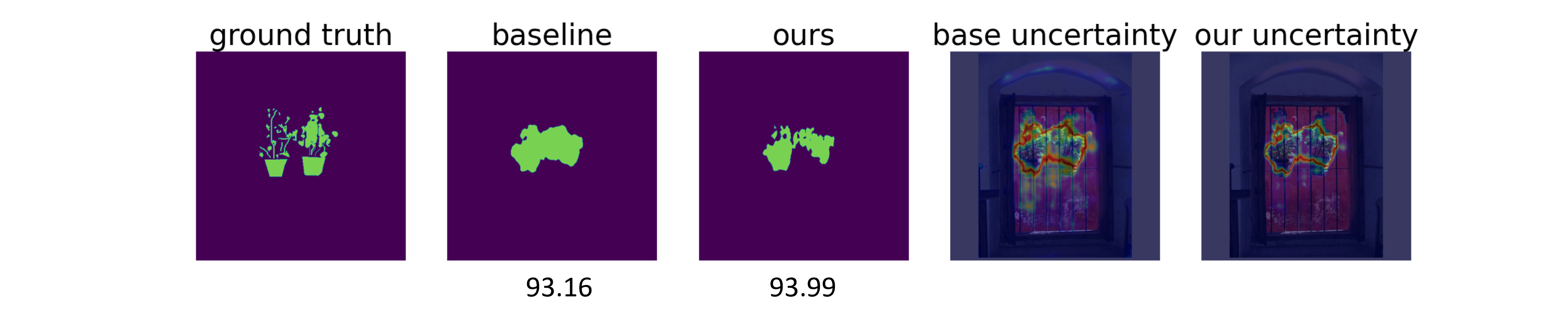
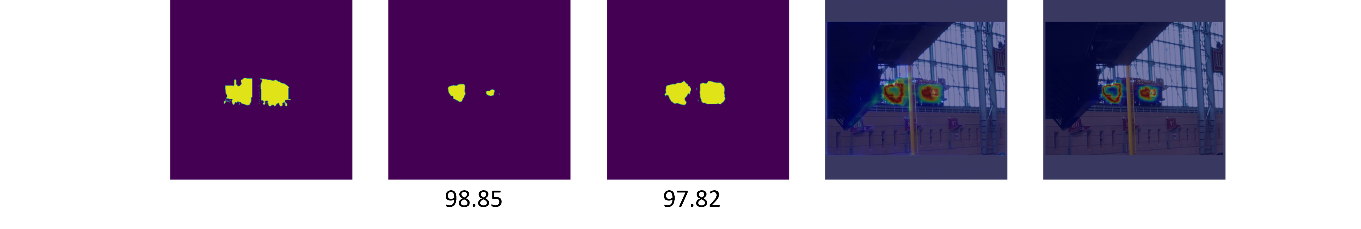
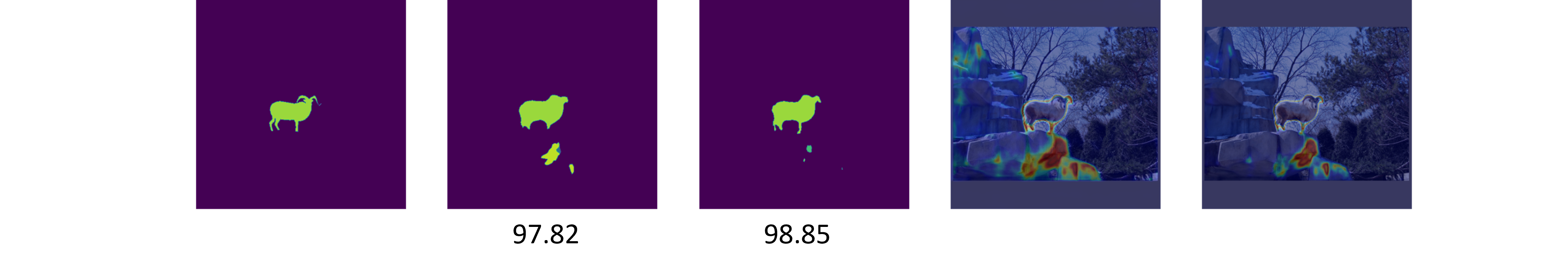
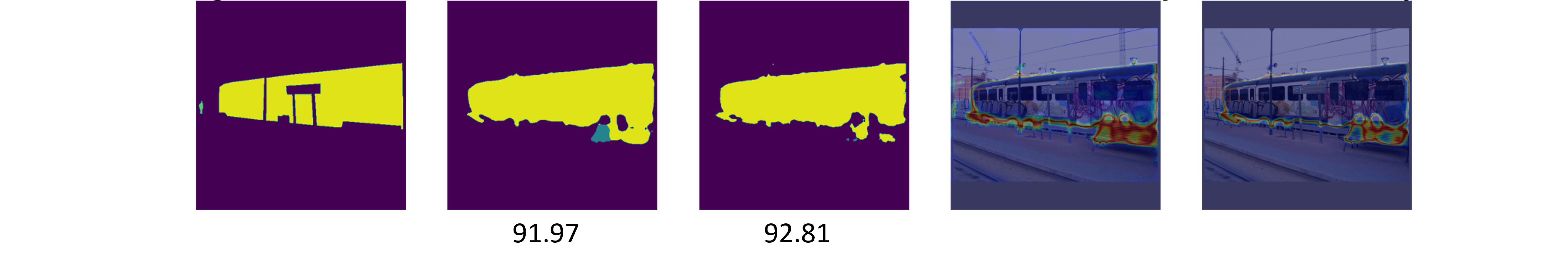
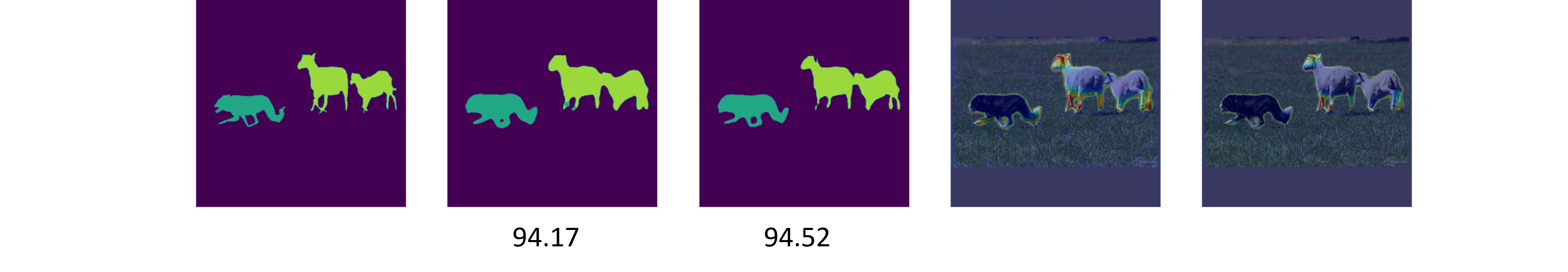
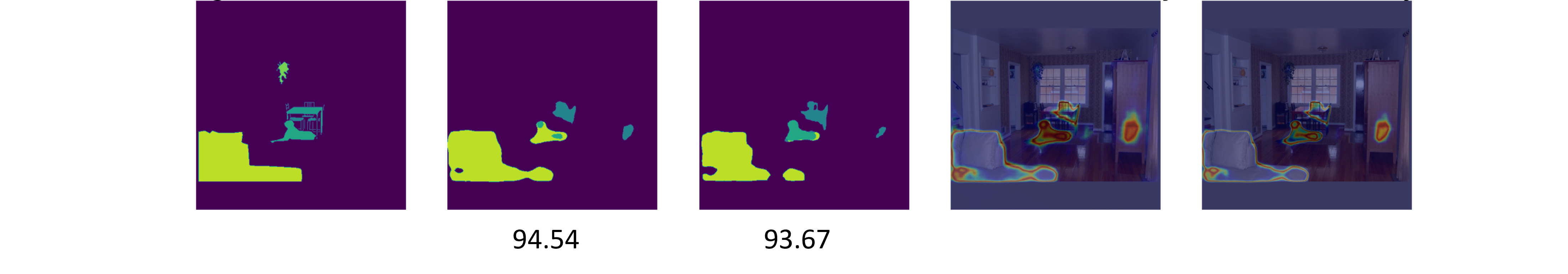
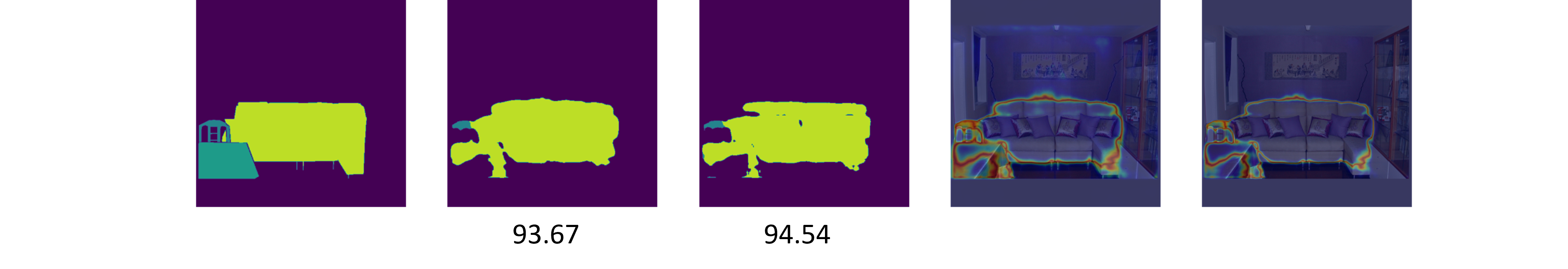
Figure H.1: Example of refined pseudo-labels, the structure is as in Fig. 3, and the numbers under the predictions show the pixel-wise accuracy of the prediction map.

References

- Arazo et al. (2020) Eric Arazo, Diego Ortego, Paul Albert, Noel E. O’Connor, and Kevin McGuinness. Pseudo-labeling and confirmation bias in deep semi-supervised learning. In International Joint Conference on Neural Networks, pages 1–8, 2020. doi: 10.1109/IJCNN48605.2020.9207304. URL https://arxiv.org/abs/1908.02983.
- Bartolomei et al. (2020) Luca Bartolomei, Lucas Teixeira, and Margarita Chli. Perception-aware path planning for UAVs using semantic segmentation. In IEEE/RSJ International Conference on Intelligent Robots and Systems (IROS), pages 5808–5815, 2020. doi: 10.1109/IROS45743.2020.9341347.
- Berthelot et al. (2019) David Berthelot, Nicholas Carlini, Ian Goodfellow, Nicolas Papernot, Avital Oliver, and Colin A. Raffel. MixMatch: a holistic approach to semi-supervised learning. In H. Wallach, H. Larochelle, A. Beygelzimer, F. d'Alché-Buc, E. Fox, and R. Garnett, editors, Advances in Neural Information Processing Systems, volume 32. Curran Associates, Inc., 2019. URL https://proceedings.neurips.cc/paper/2019/hash/1cd138d0499a68f4bb72bee04bbec2d7-Abstract.html.
- Berthelot et al. (2020) David Berthelot, Nicholas Carlini, Ekin D. Cubuk, Alex Kurakin, Kihyuk Sohn, Han Zhang, and Colin A. Raffel. ReMixMatch: semi-supervised learning with distribution matching and augmentation anchoring. In International Conference on Learning Representations, 2020. URL https://openreview.net/forum?id=HklkeR4KPB.
- Chen et al. (2018a) Liang-Chieh Chen, George Papandreou, Iasonas Kokkinos, Kevin Murphy, and Alan L. Yuille. DeepLab: semantic image segmentation with deep convolutional nets, atrous convolution, and fully connected CRFs. IEEE Transactions on Pattern Analysis and Machine Intelligence, 40(4):834–848, 2018a. doi: 10.1109/TPAMI.2017.2699184. URL https://arxiv.org/abs/1412.7062.
- Chen et al. (2018b) Liang-Chieh Chen, Yukun Zhu, George Papandreou, Florian Schroff, and Hartwig Adam. Encoder-decoder with atrous separable convolution for semantic image segmentation. In European Conference on Computer Vision (ECCV), September 2018b. URL https://openaccess.thecvf.com/content_ECCV_2018/html/Liang-Chieh_Chen_Encoder-Decoder_with_Atrous_ECCV_2018_paper.html.
- Chen et al. (2021) Xiaokang Chen, Yuhui Yuan, Gang Zeng, and Jingdong Wang. Semi-supervised semantic segmentation with cross pseudo supervision. In IEEE/CVF Conference on Computer Vision and Pattern Recognition (CVPR), pages 2613–2622, June 2021. URL https://openaccess.thecvf.com/content/CVPR2021/html/Chen_Semi-Supervised_Semantic_Segmentation_With_Cross_Pseudo_Supervision_CVPR_2021_paper.html.
- Cordts et al. (2016) Marius Cordts, Mohamed Omran, Sebastian Ramos, Timo Rehfeld, Markus Enzweiler, Rodrigo Benenson, Uwe Franke, Stefan Roth, and Bernt Schiele. The Cityscapes dataset for semantic urban scene understanding. In IEEE Conference on Computer Vision and Pattern Recognition (CVPR), June 2016. URL https://www.cv-foundation.org/openaccess/content_cvpr_2016/html/Cordts_The_Cityscapes_Dataset_CVPR_2016_paper.html.
- Dai et al. (2021) Zihang Dai, Hanxiao Liu, Quoc V. Le, and Mingxing Tan. CoAtNet: marrying convolution and attention for all data sizes. In M. Ranzato, A. Beygelzimer, Y. Dauphin, P.S. Liang, and J. Wortman Vaughan, editors, Advances in Neural Information Processing Systems, volume 34, pages 3965–3977. Curran Associates, Inc., 2021. URL https://proceedings.neurips.cc//paper/2021/hash/20568692db622456cc42a2e853ca21f8-Abstract.html.
- Dosovitskiy et al. (2021) Alexey Dosovitskiy, Lucas Beyer, Alexander Kolesnikov, Dirk Weissenborn, Xiaohua Zhai, Thomas Unterthiner, Mostafa Dehghani, Matthias Minderer, Georg Heigold, Sylvain Gelly, Jakob Uszkoreit, and Neil Houlsby. An image is worth 16x16 words: Transformers for image recognition at scale. In International Conference on Learning Representations, 2021. URL https://openreview.net/forum?id=YicbFdNTTy.
- Elliman and Lancaster (1990) Dave G. Elliman and Ian T. Lancaster. A review of segmentation and contextual analysis techniques for text recognition. Pattern Recognition, 23(3):337–346, 1990. ISSN 0031-3203. doi: https://doi.org/10.1016/0031-3203(90)90021-C. URL https://www.sciencedirect.com/science/article/pii/003132039090021C.
- Everingham et al. (2010) Mark Everingham, Luc Van Gool, Christopher K. I. Williams, John Winn, and Andrew Zisserman. The Pascal visual object classes (VOC) challenge. International Journal of Computer Vision, 88(2):303–338, June 2010. doi: 10.1007/s11263-009-0275-4. URL https://doi.org/10.1007/s11263-009-0275-4.
- French et al. (2020) Geoffrey French, Samuli Laine, Timo Aila, Michal Mackiewicz, and Graham D. Finlayson. Semi-supervised semantic segmentation needs strong, varied perturbations. In British Machine Vision Conference. BMVA Press, 2020. URL https://www.bmvc2020-conference.com/assets/papers/0680.pdf.
- Girshick (2015) Ross Girshick. Fast R-CNN. In IEEE International Conference on Computer Vision (ICCV), December 2015. URL https://openaccess.thecvf.com/content_iccv_2015/html/Girshick_Fast_R-CNN_ICCV_2015_paper.html.
- Hariharan et al. (2011) Bharath Hariharan, Pablo Arbeláez, Lubomir Bourdev, Subhransu Maji, and Jitendra Malik. Semantic contours from inverse detectors. In International Conference on Computer Vision, pages 991–998, 2011. doi: 10.1109/ICCV.2011.6126343.
- He et al. (2016) Kaiming He, Xiangyu Zhang, Shaoqing Ren, and Jian Sun. Deep residual learning for image recognition. In IEEE Conference on Computer Vision and Pattern Recognition (CVPR), June 2016. URL https://www.cv-foundation.org/openaccess/content_cvpr_2016/html/He_Deep_Residual_Learning_CVPR_2016_paper.html.
- Hinton et al. (2015) Geoffrey Hinton, Oriol Vinyals, and Jeff Dean. Distilling the knowledge in a neural network. arXiv preprint arXiv:1503.02531, 2015.
- Hu et al. (2021) Hanzhe Hu, Fangyun Wei, Han Hu, Qiwei Ye, Jinshi Cui, and Liwei Wang. Semi-supervised semantic segmentation via adaptive equalization learning. In M. Ranzato, A. Beygelzimer, Y. Dauphin, P.S. Liang, and J. Wortman Vaughan, editors, Advances in Neural Information Processing Systems, volume 34, pages 22106–22118. Curran Associates, Inc., 2021. URL https://proceedings.neurips.cc/paper/2021/file/b98249b38337c5088bbc660d8f872d6a-Paper.pdf.
- Ke et al. (2020) Zhanghan Ke, Di Qiu, Kaican Li, Qiong Yan, and Rynson W. H. Lau. Guided collaborative training for pixel-wise semi-supervised learning. In Andrea Vedaldi, Horst Bischof, Thomas Brox, and Jan-Michael Frahm, editors, European Conference on Computer Vision, pages 429–445, Cham, 2020. Springer International Publishing. ISBN 978-3-030-58601-0. URL https://www.ecva.net/papers/eccv_2020/papers_ECCV/html/1932_ECCV_2020_paper.php.
- Kirillov et al. (2023) Alexander Kirillov, Eric Mintun, Nikhila Ravi, Hanzi Mao, Chloe Rolland, Laura Gustafson, Tete Xiao, Spencer Whitehead, Alexander C. Berg, Wan-Yen Lo, Piotr Dollár, and Ross Girshick. Segment anything. arXiv preprint arXiv:2304.02643, 2023.
- Krizhevsky et al. (2012) Alex Krizhevsky, Ilya Sutskever, and Geoffrey E. Hinton. ImageNet classification with deep convolutional neural networks. In F. Pereira, C.J. Burges, L. Bottou, and K.Q. Weinberger, editors, Advances in Neural Information Processing Systems, volume 25. Curran Associates, Inc., 2012. URL https://papers.nips.cc/paper/2012/hash/c399862d3b9d6b76c8436e924a68c45b-Abstract.html.
- Laine and Aila (2016) Samuli Laine and Timo Aila. Temporal ensembling for semi-supervised learning. In International Conference on Learning Representations, 2016. URL https://openreview.net/forum?id=BJ6oOfqge.
- Lee (2013) Dong-Hyun Lee. Pseudo-label: The simple and efficient semi-supervised learning method for deep neural networks. ICML 2013 Workshop: Challenges in Representation Learning (WREPL), July 2013. URL http://deeplearning.net/wp-content/uploads/2013/03/pseudo_label_final.pdf.
- Li et al. (2022) Feng Li, Hao Zhang, Huaizhe xu, Shilong Liu, Lei Zhang, Lionel M. Ni, and Heung-Yeung Shum. Mask DINO: towards a unified transformer-based framework for object detection and segmentation. arXiv preprint, June 2022. URL https://arxiv.org/abs/2206.02777.
- Liu et al. (2022a) Shikun Liu, Shuaifeng Zhi, Edward Johns, and Andrew J. Davison. Bootstrapping semantic segmentation with regional contrast. In International Conference on Learning Representations, 2022a. URL https://openreview.net/forum?id=6u6N8WWwYSM.
- Liu et al. (2021) Yen-Cheng Liu, Chih-Yao Ma, Zijian He, Chia-Wen Kuo, Kan Chen, Peizhao Zhang, Bichen Wu, Zsolt Kira, and Peter Vajda. Unbiased teacher for semi-supervised object detection. In International Conference on Learning Representations, 2021. URL https://openreview.net/forum?id=MJIve1zgR_.
- Liu et al. (2022b) Yuyuan Liu, Yu Tian, Yuanhong Chen, Fengbei Liu, Vasileios Belagiannis, and Gustavo Carneiro. Perturbed and strict mean teachers for semi-supervised semantic segmentation. In IEEE/CVF Conference on Computer Vision and Pattern Recognition (CVPR), pages 4258–4267, June 2022b. URL https://openaccess.thecvf.com/content/CVPR2022/html/Liu_Perturbed_and_Strict_Mean_Teachers_for_Semi-Supervised_Semantic_Segmentation_CVPR_2022_paper.html.
- Milioto et al. (2018) Andres Milioto, Philipp Lottes, and Cyrill Stachniss. Real-time semantic segmentation of crop and weed for precision agriculture robots leveraging background knowledge in CNNs. In IEEE International Conference on Robotics and Automation (ICRA), pages 2229–2235, 2018. doi: 10.1109/ICRA.2018.8460962. URL https://arxiv.org/abs/1709.06764.
- Miyato et al. (2018) Takeru Miyato, Shin-Ichi Maeda, Masanori Koyama, and Shin Ishii. Virtual adversarial training: a regularization method for supervised and semi-supervised learning. IEEE Transactions on Pattern Analysis and Machine Intelligence, 41(8):1979–1993, 2018. doi: 10.1109/TPAMI.2018.2858821. URL https://ieeexplore.ieee.org/abstract/document/8417973.
- Nekrasov et al. (2021) Alexey Nekrasov, Jonas Schult, Or Litany, Bastian Leibe, and Francis Engelmann. Mix3d: Out-of-context data augmentation for 3d scenes. 3DV 2021, 2021.
- Ouali et al. (2020) Yassine Ouali, Céline Hudelot, and Myriam Tami. Semi-supervised semantic segmentation with cross-consistency training. In IEEE/CVF Conference on Computer Vision and Pattern Recognition (CVPR), June 2020. URL https://openaccess.thecvf.com/content_CVPR_2020/html/Ouali_Semi-Supervised_Semantic_Segmentation_With_Cross-Consistency_Training_CVPR_2020_paper.html.
- Rasmus et al. (2015) Antti Rasmus, Mathias Berglund, Mikko Honkala, Harri Valpola, and Tapani Raiko. Semi-supervised learning with ladder networks. In C. Cortes, N. Lawrence, D. Lee, M. Sugiyama, and R. Garnett, editors, Advances in Neural Information Processing Systems, volume 28. Curran Associates, Inc., 2015. URL https://papers.nips.cc/paper/2015/hash/378a063b8fdb1db941e34f4bde584c7d-Abstract.html.
- Rizve et al. (2021) Mamshad Nayeem Rizve, Kevin Duarte, Yogesh S. Rawat, and Mubarak Shah. In defense of pseudo-labeling: An uncertainty-aware pseudo-label selection framework for semi-supervised learning. In International Conference on Learning Representations, 2021. URL https://openreview.net/forum?id=-ODN6SbiUU.
- Russakovsky et al. (2015) Olga Russakovsky, Jia Deng, Hao Su, Jonathan Krause, Sanjeev Satheesh, Sean Ma, Zhiheng Huang, Andrej Karpathy, Aditya Khosla, Michael Bernstein, Alexander C. Berg, and Li Fei-Fei. ImageNet large scale visual recognition challenge. International Journal of Computer Vision, 115(3):211–252, 2015. doi: 10.1007/s11263-015-0816-y.
- Scheffer et al. (2001) Tobias Scheffer, Christian Decomain, and Stefan Wrobel. Active hidden Markov models for information extraction. In Frank Hoffmann, David J. Hand, Niall Adams, Douglas Fisher, and Gabriela Guimaraes, editors, Advances in Intelligent Data Analysis, pages 309–318, Berlin, Heidelberg, 2001. Springer Berlin Heidelberg. ISBN 978-3-540-44816-7. URL https://link.springer.com/chapter/10.1007/3-540-44816-0_31.
- Shin et al. (2021) Gyungin Shin, Weidi Xie, and Samuel Albanie. All you need are a few pixels: Semantic segmentation with PixelPick. In Proceedings of the IEEE/CVF International Conference on Computer Vision (ICCV) Workshops, pages 1687–1697, October 2021. URL https://openaccess.thecvf.com/content/ICCV2021W/ILDAV/html/Shin_All_You_Need_Are_a_Few_Pixels_Semantic_Segmentation_With_ICCVW_2021_paper.html.
- Sohn et al. (2020a) Kihyuk Sohn, David Berthelot, Nicholas Carlini, Zizhao Zhang, Han Zhang, Colin A. Raffel, Ekin Dogus Cubuk, Alexey Kurakin, and Chun-Liang Li. FixMatch: simplifying semi-supervised learning with consistency and confidence. In H. Larochelle, M. Ranzato, R. Hadsell, M. F. Balcan, and H. Lin, editors, Advances in Neural Information Processing Systems, volume 33, pages 596–608. Curran Associates, Inc., 2020a. URL https://proceedings.neurips.cc/paper/2020/hash/06964dce9addb1c5cb5d6e3d9838f733-Abstract.html.
- Sohn et al. (2020b) Kihyuk Sohn, Zizhao Zhang, Chun-Liang Li, Han Zhang, Chen-Yu Lee, and Tomas Pfister. A simple semi-supervised learning framework for object detection. arXiv preprint arXiv:2005.04757, 2020b.
- Tarvainen and Valpola (2017) Antti Tarvainen and Harri Valpola. Mean teachers are better role models: Weight-averaged consistency targets improve semi-supervised deep learning results. In I. Guyon, U. V. Luxburg, S. Bengio, H. Wallach, R. Fergus, S. Vishwanathan, and R. Garnett, editors, Advances in Neural Information Processing Systems, volume 30. Curran Associates, Inc., 2017. URL https://proceedings.neurips.cc/paper/2017/hash/68053af2923e00204c3ca7c6a3150cf7-Abstract.html.
- Toussaint (1978) Godfried T. Toussaint. The use of context in pattern recognition. Pattern Recognition, 10(3):189–204, 1978. ISSN 0031-3203. doi: https://doi.org/10.1016/0031-3203(78)90027-4. URL https://www.sciencedirect.com/science/article/pii/0031320378900274. The Proceedings of the IEEE Computer Society Conference.
- Van Etten et al. (2018) Adam Van Etten, Dave Lindenbaum, and Todd M. Bacastow. SpaceNet: a remote sensing dataset and challenge series. arXiv preprint, June 2018. URL https://arxiv.org/abs/1807.01232.
- Vaswani et al. (2017) Ashish Vaswani, Noam Shazeer, Niki Parmar, Jakob Uszkoreit, Llion Jones, Aidan N. Gomez, Lukasz Kaiser, and Illia Polosukhin. Attention is all you need. arXiv preprint, 2017.
- Wang et al. (2021) He Wang, Yezhen Cong, Or Litany, Yue Gao, and Leonidas J. Guibas. 3DIoUMatch: leveraging IoU prediction for semi-supervised 3D object detection. In Proceedings of the IEEE/CVF Conference on Computer Vision and Pattern Recognition (CVPR), pages 14615–14624, June 2021. URL https://openaccess.thecvf.com/content/CVPR2021/html/Wang_3DIoUMatch_Leveraging_IoU_Prediction_for_Semi-Supervised_3D_Object_Detection_CVPR_2021_paper.html.
- Wang et al. (2020) Qilong Wang, Banggu Wu, Pengfei Zhu, Peihua Li, Wangmeng Zuo, and Qinghua Hu. ECA-Net: Efficient channel attention for deep convolutional neural networks. In Proceedings of the IEEE/CVF conference on computer vision and pattern recognition, pages 11534–11542, 2020.
- Wang et al. (2023) Yidong Wang, Hao Chen, Qiang Heng, Wenxin Hou, Yue Fan, Zhen Wu, Jindong Wang, Marios Savvides, Takahiro Shinozaki, Bhiksha Raj, Bernt Schiele, and Xing Xie. FreeMatch: self-adaptive thresholding for semi-supervised learning. In International Conference on Learning Representations, 2023. URL https://openreview.net/forum?id=PDrUPTXJI_A.
- Wang et al. (2022) Yuchao Wang, Haochen Wang, Yujun Shen, Jingjing Fei, Wei Li, Guoqiang Jin, Liwei Wu, Rui Zhao, and Xinyi Le. Semi-supervised semantic segmentation using unreliable pseudo labels. In IEEE/CVF International Conference on Computer Vision and Pattern Recognition (CVPR), 2022. URL https://openaccess.thecvf.com/content/CVPR2022/html/Wang_Semi-Supervised_Semantic_Segmentation_Using_Unreliable_Pseudo-Labels_CVPR_2022_paper.html.
- Xie et al. (2020) Qizhe Xie, Zihang Dai, Eduard Hovy, Thang Luong, and Quoc V. Le. Unsupervised data augmentation for consistency training. In H. Larochelle, M. Ranzato, R. Hadsell, M. F. Balcan, and H. Lin, editors, Advances in Neural Information Processing Systems, volume 33, pages 6256–6268. Curran Associates, Inc., 2020. URL https://proceedings.neurips.cc/paper/2020/hash/44feb0096faa8326192570788b38c1d1-Abstract.html.
- Xu et al. (2022) Hai-Ming Xu, Lingqiao Liu, Qiuchen Bian, and Zhen Yang. Semi-supervised semantic segmentation with prototype-based consistency regularization. In Advances in Neural Information Processing Systems (NeurIPS), 2022.
- Yang et al. (2022a) Fan Yang, Kai Wu, Shuyi Zhang, Guannan Jiang, Yong Liu, Feng Zheng, Wei Zhang, Chengjie Wang, and Long Zeng. Class-aware contrastive semi-supervised learning. In IEEE/CVF Conference on Computer Vision and Pattern Recognition (CVPR), pages 14421–14430, June 2022a. URL https://openaccess.thecvf.com/content/CVPR2022/html/Yang_Class-Aware_Contrastive_Semi-Supervised_Learning_CVPR_2022_paper.html.
- Yang et al. (2022b) Lihe Yang, Wei Zhuo, Lei Qi, Yinghuan Shi, and Yang Gao. ST++: make self-training work better for semi-supervised semantic segmentation. In IEEE/CVF Conference on Computer Vision and Pattern Recognition (CVPR), pages 4268–4277, June 2022b. URL https://openaccess.thecvf.com/content/CVPR2022/html/Yang_ST_Make_Self-Training_Work_Better_for_Semi-Supervised_Semantic_Segmentation_CVPR_2022_paper.html.
- Yang et al. (2023a) Lihe Yang, Lei Qi, Litong Feng, Wayne Zhang, and Yinghuan Shi. Revisiting weak-to-strong consistency in semi-supervised semantic segmentation. In Proceedings of the IEEE/CVF Conference on Computer Vision and Pattern Recognition (CVPR), pages 7236–7246, June 2023a. URL https://openaccess.thecvf.com/content/CVPR2023/html/Yang_Revisiting_Weak-to-Strong_Consistency_in_Semi-Supervised_Semantic_Segmentation_CVPR_2023_paper.html.
- Yang et al. (2023b) Lihe Yang, Lei Qi, Litong Feng, Wayne Zhang, and Yinghuan Shi. Revisiting weak-to-strong consistency in semi-supervised semantic segmentation. In CVPR, 2023b.
- Yun et al. (2019) Sangdoo Yun, Dongyoon Han, Seong Joon Oh, Sanghyuk Chun, Junsuk Choe, and Youngjoon Yoo. CutMix: regularization strategy to train strong classifiers with localizable features. In IEEE/CVF International Conference on Computer Vision (ICCV), October 2019. URL https://openaccess.thecvf.com/content_ICCV_2019/html/Yun_CutMix_Regularization_Strategy_to_Train_Strong_Classifiers_With_Localizable_Features_ICCV_2019_paper.html.
- Zagoruyko et al. (2016) Sergey Zagoruyko, Adam Lerer, Tsung-Yi Lin, Pedro O. Pinheiro, Sam Gross, Soumith Chintala, and Piotr Dollár. A MultiPath network for object detection. In Edwin R. Hancock Richard C. Wilson and William A. P. Smith, editors, Proceedings of the British Machine Vision Conference (BMVC), pages 15.1–15.12. BMVA Press, September 2016. ISBN 1-901725-59-6. doi: 10.5244/C.30.15. URL https://dx.doi.org/10.5244/C.30.15.
- Zhang et al. (2021) Bowen Zhang, Yidong Wang, Wenxin Hou, Hao Wu, Jindong Wang, Manabu Okumura, and Takahiro Shinozaki. Flexmatch: Boosting semi-supervised learning with curriculum pseudo labeling. In M. Ranzato, A. Beygelzimer, Y. Dauphin, P.S. Liang, and J. Wortman Vaughan, editors, Advances in Neural Information Processing Systems, volume 34, pages 18408–18419. Curran Associates, Inc., 2021. URL https://proceedings.neurips.cc/paper/2021/hash/995693c15f439e3d189b06e89d145dd5-Abstract.html.
- Zhao et al. (2020) Na Zhao, Tat-Seng Chua, and Gim Hee Lee. SESS: self-ensembling semi-supervised 3D object detection. In Proceedings of the IEEE/CVF Conference on Computer Vision and Pattern Recognition (CVPR), June 2020. URL https://openaccess.thecvf.com/content_CVPR_2020/html/Zhao_SESS_Self-Ensembling_Semi-Supervised_3D_Object_Detection_CVPR_2020_paper.html.
- Zhong et al. (2021) Yuanyi Zhong, Bodi Yuan, Hong Wu, Zhiqiang Yuan, Jian Peng, and Yu-Xiong Wang. Pixel contrastive-consistent semi-supervised semantic segmentation. In IEEE/CVF International Conference on Computer Vision (ICCV), pages 7273–7282, October 2021. URL https://openaccess.thecvf.com/content/ICCV2021/html/Zhong_Pixel_Contrastive-Consistent_Semi-Supervised_Semantic_Segmentation_ICCV_2021_paper.html.
- Zong et al. (2022) Zhuofan Zong, Guanglu Song, and Yu Liu. DETRs with collaborative hybrid assignments training. arXiv preprint, November 2022. URL https://arxiv.org/abs/2211.12860.
- Zou et al. (2021) Yuliang Zou, Zizhao Zhang, Han Zhang, Chun-Liang Li, Xiao Bian, Jia-Bin Huang, and Tomas Pfister. PseudoSeg: designing pseudo labels for semantic segmentation. In International Conference on Learning Representations, 2021. URL https://openreview.net/forum?id=-TwO99rbVRu.