Estimating Changepoints in Extremal Dependence, Applied to Aviation Stock Prices During COVID-19 Pandemic

Abstract

The dependence in the tails of the joint distribution of two random variables is measured using $\chi$-measure. This work is motivated by the structural changes in $\chi$-measure between the daily return rates of the two largest Indian airlines in 2019, IndiGo and SpiceJet, during the COVID-19 pandemic. We model the daily maximum return rate vectors (potentially transformed) using the bivariate Hüsler-Reiss (BHR) distribution,  which is the only possible non-degenerate limiting distribution of a renormalized element-wise block maxima of a sequence of bivariate Gaussian random vectors. To estimate the changepoint in the $\chi$-measure of the BHR distribution, we explore the changepoint detection procedures based on Likelihood Ratio Test (LRT) and Modified Information Criterion (MIC). We obtain critical values and power curves of the LRT and MIC test statistics for low through high values of $\chi$-measure. We also explore the consistency of the estimators of the changepoint based on LRT and MIC numerically. In our data application, the most prominent changepoint detected by LRT and MIC coincides with the announcement of the first phase of lockdown declared by the Government of India, which is realistic; thus, our study would be beneficial for portfolio optimization in the case of future pandemic situations.

1 Introduction

The COVID-19 pandemic had a profound and disruptive impact on a global scale, causing not only a substantial loss of human lives but also significant economic turmoil. Nearly every industry faced adverse consequences as a result, including the aviation sector. The outbreak of the pandemic triggered a severe decline in air travel demand, as countries implemented travel restrictions and lockdown measures to curb the spread of the virus. Extensive research, such as the study conducted by the International Civil Aviation Organization (ICAO, 2020) on the effects of COVID-19 on worldwide Civil Aviation, has examined these repercussions. Indian airlines encountered numerous challenges during this unprecedented period, as highlighted in Sidhu and Shukla (2021) and Agrawal (2021), who examined the specific difficulties faced by Indian airlines due to the pandemic. The imposition of domestic and international flight suspensions for several months by the Government of India had a significant financial impact on airlines, leading to layoffs, salary cuts, and even bankruptcies (TOI, 2020).

The two airlines IndiGo and SpiceJet have played crucial roles in fostering the growth of the Indian aviation sector. These airlines have effectively increased the accessibility and affordability of air travel for a broader range of people. Operating in a highly competitive market, they have continuously expanded their flight routes, enhanced services, and taken innovative features to attract passengers (Banerji et al., 2016). Thus, it is unavoidable that there exists an interdependence within their businesses. Analyzing the share prices of the two companies over a period of time allows one to gauge the market’s perception of the companies and their financial performances. There are several parameters to consider while using share prices for performance evaluation, such as historical share price trends, relative performance, market index comparisons, and the impact of dividends and stock splits. The traders emphasize the importance of buying low and selling high while aiming to generate profits. This principle underscores the significance of timing and strategic decision-making in the context of stock market investments (Cartea et al., 2014). During the first phase of the lockdown, the world witnessed a significant decline in the stock market for many shares, primarily caused by reduced investments (Gormsen and Koijen, 2020). While analyzing daily average stock prices gives an understanding of the bulk of the distribution of the share prices, our goal is to focus on understanding the upper tail behavior of stock prices, which is a more precise indicator of their interdependence at the sell positions. Various companies employed diverse strategies to mitigate substantial losses during the pandemic (BT, 2020). As a result, their tail interdependence, i.e., the tendency of selling both SpiceJet and IndiGo stocks simultaneously in high amounts, could have experienced significant change during the COVID-19 pandemic. To analyze them effectively, we employ extreme value theory (EVT) and changepoint analysis.

In recent years, EVT has emerged as one of the most crucial fields of study in different scientific disciplines (Coles, 2001; Davison and Huser, 2015). The main applications of EVT are in areas such as portfolio management in actuarial studies (Huang et al., 2020), financial risk assessment (Chavez-Demoulin et al., 2016), telecom traffic prediction (Molina-Garcia et al., 2008), and detection of meteorological changes (Zwiers and Kharin, 1998). In financial extremes, Rocco (2014) showed that a portfolio is more affected by a few extreme movements in the market than by the sum of many small-scale shifts. While the majority of EVT focuses on methods for analyzing univariate extremes, Tawn (1988) and Tiago de Oliveira (1989) introduced the statistical methodology for bivariate extremes, and Coles and Tawn (1994) further studied multivariate extremes. While the Pearson correlation coefficient measures dependence in the bulk of the joint distribution of two random variables, $\chi$-measure (Sibuya, 1960) assesses the dependence in tails. While a bivariate Gaussian distribution is the most common model for bivariate responses, its components are asymptotically independent for any non-trivial choice of the Pearson correlation coefficient (Sibuya, 1960). In this context, Hüsler and Reiss (1989) obtained the limiting distribution of block maxima of bivariate Gaussian distribution under certain assumptions on the correlation between the components, and their bivariate model is known as the bivariate Hüsler-Reiss (BHR) distribution. The BHR distribution and its infinite-dimensional case called Brown-Resnick process (Brown and Resnick, 1977) have been used in numerous studies in the context of bivariate, multivariate, as well as spatial extreme value analysis (Kabluchko et al., 2009; Huser and Davison, 2013). Besides, the BHR distribution is a building block of the high-dimensional graphical models for extremes (Engelke and Hitz, 2020; Engelke and Ivanovs, 2021).

A changepoint is a place or time where the statistical properties of a sequence of observations change; in other words, the observations before and after the changepoint follow different probability distributions (Chen and Gupta, 2012; Killick and Eckley, 2014). We can use this information for prediction, monitoring, and decision-making purposes. Changepoint estimation or changepoint mining is common in many fields such as financial time series data (Thies and Molnár, 2018), environmental studies (Reeves et al., 2007), genome research (Muggeo and Adelfio, 2011), signal processing (Lavielle, 2005), quality control (Lai, 1995), and medical research (Bosc et al., 2003). During the 1950s, Page (1955) first proposed a methodology for detecting only one change in a one-parameter (location-type) model. For a univariate Gaussian distribution, Chernoff and Zacks (1964) and Gardner (1969) studied changepoint detection for the mean component, and Hsu (1977) studied a similar problem for the variance.

While their studies were limited to a single parameter and a single changepoint scenario, Hawkins (1992) proposed a novel approach for detecting a single shift in any known function of the unknown mean and covariance of an arbitrary multivariate distribution, and Inclán (1993) proposed a multiple changepoint detection procedure for the variance of a Gaussian distribution using posterior odds in a Bayesian setting. Lerman and Schechtman (1989) discussed techniques and results on changepoint estimation for the correlation coefficient of the bivariate Gaussian distribution. Among the various methods for detecting changepoints, the Likelihood Ratio Test (LRT) and Modified Information Criteria (MIC) are among the most common approaches. A detailed discussion on parametric and non-parametric changepoint detection approaches is in Csörgö and Horváth (1997) and Chen and Gupta (2012).

Worsley (1979) examined the utilization of LRT to identify shifts or changes in the location of normal populations, while Worsley (1983) focused on studying the power of LRT for detecting changes in binomial probabilities. Later, Srivastava and Worsley (1986) investigated LRT for identifying changepoints in a multivariate setting, and Ramanayake and Gupta (2003) discussed the detection of epidemic changes using LRT for exponential distribution. Further, Zhao et al. (2013) studied detecting changepoints in two-phase linear regression models using LRT, and Said et al. (2017) used LRT for detecting changepoints in a sequence of univariate skew-normal distributed random variables. Without imposing any parametric model assumption, Zou et al. (2007) proposed a changepoint detection procedure based on the empirical likelihood, and its asymptotic properties are justified by the work of Owen (1988). As an alternative to LRT, Chen and Gupta (1997), Chen et al. (2006), Hasan et al. (2014), Ngunkeng and Ning (2014), and Cai et al. (2016) used the information criteria approach for changepoint detection. Specifically, Chen et al. (2006) proposed Modified Information Criterion (MIC) and showed that MIC has simple asymptotic behaviors and is consistent. While LRT generally performs better in detecting changepoints occurring near the middle of the data sequence, MIC includes some correction terms that allow better performance in detecting changepoints occurring at the very beginning or at the very end of the data. Among its applications, Said et al. (2019) and Tian et al. (2023) used MIC for changepoint estimation in case of skew-normal and Kumaraswamy distributions, respectively.

In the context of changepoint estimation for a sequence of extremes, Leadbetter et al. (1983) and Embrechts et al. (1997) studied some theoretical properties of some test statistics. In a book chapter, Dias and Embrechts (2004) briefly discussed LRT for analyzing changes in the extreme value copulas and illustrated it for the bivariate Gumbel copula. Jarušková and Rencová (2008) discussed LRT for detecting a changepoint in the location parameter of annual maxima and minima series and described some methods for finding critical values. Instead of focusing on block maxima, Dierckx and Teugels (2010) discussed LRT for detecting changes in the shape parameter of the generalized Pareto distribution, which is the only possible limiting distribution of high-threshold exceedances. While the previous approaches focused on a frequentist analysis of extreme values, do Nascimento and e Silva (2017) discussed a Bayesian method to identify changepoints in a sequence of extremes. For detecting changepoints in financial extremes, Lattanzi and Leonelli (2021) discussed a Bayesian approach for analyzing threshold exceedances using a generalized Pareto distribution while modeling the bulk of the distribution using a finite mixture of gamma distributions.

Similar to the Pearson correlation coefficient for analyzing dependence in the bulk of the joint distribution of two random variables, the strength of the dependence in tails is measured using extremal dependence or $\chi$-measure. Our purpose is to identify structural changes in the $\chi$-measure between the daily stock return rates of the two largest Indian airlines, IndiGo and SpiceJet, during the COVID-19 pandemic in 2019. To accomplish this, we discuss necessary preprocessing steps, including transforming the daily maximum return rate series so that they jointly follow the BHR distribution. The main objective of this paper is to estimate the point at which a change occurs in the $\chi$-measure of the BHR distribution. Given the one-to-one correspondence between the dependence-related parameter of the BHR distribution and its $\chi$-measure, we explore a changepoint detection procedure utilizing LRT and MIC to achieve our goal. To assess the performance of these methods in practical settings with limited data samples, we numerically investigate their effectiveness. Since closed-form expressions for the finite sample distributions of LRT and MIC do not exist, we derive critical values and assess the power of the hypothesis testing problem across a range of low to high values of $\chi$-measure. In our real data analysis, we explore the likelihood of different changepoints from the beginning of the COVID-19 pandemic until the end of the third wave based on both LRT and MIC.

We organize the paper as follows. In Section 2, we discuss a summary of univariate and bivariate extreme value theory, quantification of extremal dependence, and the definition of the BHR distribution. Section 3 discusses the Indian aviation stock price dataset and some exploratory analyses. We describe LRT and MIC for detecting the most crucial changepoint in a sequence of BHR-distributed bivariate random vectors in Section 4. Section 5 discusses results on critical values and power comparison between LRT and MIC based on an extensive simulation study. In Section 6, we apply our methodology to analyze the stock prices of SpiceJet and IndiGo during the COVID-19 pandemic. Section 7 concludes and discusses some scopes for future research.

2 Background on Extreme Value Theory

2.1 Univariate and Bivariate Extreme Value Distributions

The Extreme Value Theory (EVT) deals with extreme observations; they are usually defined as block maxima (e.g., annual maxima of daily observations) or threshold exceedances (e.g., the observations above the $0.98^{th}$ data quantile). We stick to the first type of definition in our case. Under both definitions, the important aspect of EVT lies in describing the tail behavior of a stochastic process. In mathematical notations, consider $X_{1},X_{2},\ldots$, a sequence of independent random variables, where $X_{i}$’s are measured on a regular time scale, following a common continuous cumulative distribution function (CDF) $F_{0}(\cdot)$. The main goal of EVT is to study the asymptotic behavior of $M_{n}=\max_{n}\{X_{1},X_{2},\ldots,X_{n}\}$. The CDF of $M_{n}$ is given by $\textrm{P}(M_{n}\leq z)=F_{0}(z)^{n}$. But, in practice, $F_{0}(\cdot)$ is generally unknown. One approach would be estimating it from observed data in case the full sequence of observations is available; however, a small overestimation or underestimation usually influences the final inference substantially.

In this context, the celebrated Fisher-Tippett theorem (Fisher and Tippett, 1928) states that for any arbitrary CDF $F_{0}(\cdot)$, if there exist sequences of real numbers $\{a^{0}_{n}\}$ and $\{b^{0}_{n}\}$ and a non-degenerate CDF $G_{0}(\cdot)$ satisfying $\lim_{n\rightarrow\infty}F_{0}^{n}(a^{0}_{n}x+b^{0}_{n})=G_{0}(x)$ pointwise, then $G_{0}(\cdot)$ must belong to either Gumbel, Fréchet, or Weibull families. Here, $F_{0}(\cdot)$ is said to belong to the Domain of Attraction of $G_{0}(\cdot)$, and $a^{0}_{n}\in\mathbb{R}^{+}$ and $b^{0}_{n}\in\mathbb{R}$ are normalizing constants. Combining these three categories, $G_{0}(\cdot)$ is the CDF of the generalized extreme value (GEV) distribution given by

$$G_{0}(y)\;=\;\exp\left[-\left\{1\;+\;\xi\left(\frac{y-\mu}{\sigma}\right)\right\}_{+}^{-1/\xi}\right],$$ (1)

where $\mu\in\mathbb{R}$, $\sigma\in\mathbb{R}^{+}$, and $\xi\in\mathbb{R}$ are the location, scale, and shape parameters of the GEV distribution, and $x_{+}=\max\{x,0\}$. Depending on whether the shape parameter $\xi$ is zero, positive, or negative, the GEV family is called the Gumbel family, Fréchet family, or Weibull family, respectively. We denote the distribution with CDF $G_{0}(\cdot)$ by $\textrm{GEV}(\mu,\sigma,\xi)$, and in practice, we assume $M_{n}\sim\textrm{GEV}(\mu,\sigma,\xi)$ in a limiting sense. The centering (through $b^{0}_{n}$) and scaling (through $a^{0}_{n}$) of $M_{n}$ in the Fisher-Tippett theorem are assumed to be adjusted by the parameters $\mu$ and $\sigma$, respectively.

Multivariate extreme value theory focuses on the case where multiple sequences of random variables are available and we are interested in assessing the joint asymptotic behavior of the block maxima for all sequences. For our purpose, we stick to the bivariate extremes scenario. Suppose $\{(X_{1},Y_{1}),(X_{2},Y_{2}),\ldots\}$ is a sequence of IID bivariate random vectors having a common continuous CDF $F(\cdot,\cdot)$. The classical theory for characterizing the extremal behavior of bivariate extremes is based on the asymptotic behavior of the component-wise block maxima vector $\bm{M}_{n}=(M_{X,n},M_{Y,n})^{\prime}$, where $M_{X,n}=\max_{1\leq i\leq n}\{X_{i}\}$ and $M_{Y,n}=\max_{1\leq i\leq n}\{Y_{i}\}$. Extending the Fisher-Tippett theorem for bivariate cases, Campbell and Tsokos (1973) stated that if there exist real sequences $\{a_{n}\}$, $\{b_{n}\}$, $\{c_{n}\}$ and $\{d_{n}\}$, where $a_{n},c_{n}\in\mathbb{R}^{+}$ for all $n$, and a bivariate non-degenerate CDF $G(\cdot,\cdot)$ that satisfy $\lim_{n\rightarrow\infty}F^{n}(a_{n}x+b_{n},c_{n}y+d_{n})=G(x,y)$ pointwise, then $G(\cdot,\cdot)$ is called the bivariate GEV distribution. Here, the standard Fisher-Tippett theorem applies to both $\{X_{1},X_{2},\ldots\}$ and $\{Y_{1},Y_{2},\ldots\}$, and the limiting CDFs of renormalized $M_{X,n}$ and $M_{Y,n}$ are of the form (1). Suppose, $M_{X,n}\sim\textrm{GEV}(\mu_{X},\sigma_{X},\xi_{X})$ and $M_{Y,n}\sim\textrm{GEV}(\mu_{Y},\sigma_{Y},\xi_{Y})$ in a limiting sense. The CDF $G(\cdot,\cdot)$ can be written as

$$G(x,y)=\exp\{-V(\widetilde{x},\widetilde{y})\},$$ (2)

where $\widetilde{x}=[1+\xi_{X}(x-\mu_{X})/\sigma_{X}]^{1/\xi_{X}}$ and $\widetilde{y}=[1+\xi_{Y}(y-\mu_{Y})/\sigma_{Y}]^{1/\xi_{Y}}$. Here, we assume $[1+\xi_{X}(x-\mu_{X})/\sigma_{X}]>0$, $1+\xi_{Y}(y-\mu_{Y})/\sigma_{Y}>0$ and $V(\widetilde{x},\widetilde{y})=2\int_{0}^{1}\max\left\{w/\widetilde{x},(1-w)/\widetilde{y}\right\}\mathrm{d}\widetilde{G}(w)$, where $\widetilde{G}(\cdot)$ is a CDF on $[0,1]$ satisfying the mean constraint $\int_{0}^{1}w\mathrm{d}\widetilde{G}(w)=1/2$. Here, $V(\cdot,\cdot)$ is called the exponent measure of $G(\cdot,\cdot)$.

2.2 Extremal dependence and F-madogram

For certain bivariate CDFs with finite second moments, even if the two components of the corresponding bivariate random vector are highly correlated, i.e., the dependence in the bulk of the joint distribution is strong, the dependence in the tails can be weak or negligible. Similar to Pearson’s correlation for analyzing dependence in the bulk of the joint distribution, the most common metric for measuring dependence in the tails is called extremal dependence or $\chi$-measure introduced by Sibuya (1960). This measure does not require the second moments to be necessarily finite.

For a bivariate random vector with two components $X$ and $Y$, and marginal CDFs $F_{X}(\cdot)$ and $F_{Y}(\cdot)$, the $\chi$-measure at a quantile level $u$ is defined as

$$\chi(u)=\textrm{P}\{F_{Y}(Y)>u|F_{X}(X)>u\},~{}~{}~{}~{}u\in(0,1),$$ (3)

while the limiting $\chi$-measure is defined as $\chi=\lim_{u\uparrow 1}\chi(u)$. Here, $\chi(u)$ is not uniquely defined and dependent on $u$. Thus, for a unique measure of extremal dependence, we use $\chi$ unless specified. Intuitively, a high value of $\chi$ indicates the tendency of $Y$ being extremely large given $X$ is extremely large. If $\chi\in(0,1]$, we call $X$ and $Y$ to be asymptotically dependent, while for $\chi=0$, $X$ and $Y$ are said to be asymptotically independent. In (3), $X$ and $Y$ are interchangeable. More details are in Coles (2001).

For a bivariate GEV distribution, (2) and (3) are linked through the equation

$$\chi(u)\;=\;2\;-\;V(1,\;1),$$ (4)

uniformly for $u\in(0,1)$, and thus, $\chi=2-V(1,1)$; see Chapter 8 of Coles (2001). In case IID replications of $(X,Y)^{\prime}$ are available, $\chi(u)$ can be computed empirically. However, the concept of $\chi$-measure can be extended from a bivariate setting to a stochastic process setting. For a stationary extremal time series $\{Z_{1},Z_{2},\ldots\}$ with a common marginal CDF $F(\cdot)$, the $\chi$-measure at a temporal lag $h=1,2,\ldots$ can be investigated using $F$-madogram (Cooley et al., 2006) given by $\nu_{h}=E\left[|F(Z_{t+h})-F(Z_{t})|\right]/2$ for any $t$. Then, the $\chi$-measure at lag $h$, say $\chi_{h}$, satisfies

$$\chi_{h}=2-\left(\frac{1+2\nu_{h}}{1-2\nu_{h}}\right).$$ (5)

In practice, for testing temporal extremal independence, we calculate $\chi_{h}$ empirically and check whether the values are close to zero. If $\chi_{h}$ are negligible for all $h$, we can safely ignore extremal dependence and model $\{Z_{1},Z_{2},\ldots\}$ as IID observations.

2.3 Bivariate Hüsler-Reiss Distribution

For a sequence of independent random variables $X_{1},X_{2},\ldots$ measured on a regular time scale and with a common CDF $F_{0}(\cdot)$, if $F_{0}(\cdot)=\Phi(\cdot)$–the standard Gaussian CDF, $G_{0}(\cdot)$ in (1) belongs to the Gumbel family (David and Nagaraja, 2004), i.e., $\xi=0$, which is defined in a limiting sense $\xi\rightarrow 0$, and we have $G_{0}(y)=\exp(-\exp[-y]),~{}y\in\mathbb{R}$. Here, for a sequence $\{b_{n}\}$ satisfying $b_{n}=n\phi(b_{n})$, where $\phi(\cdot)$ denotes a standard Gaussian density, we have $\lim_{n\uparrow\infty}\Phi^{n}\left(b_{n}+x/b_{n}\right)=\exp(-\exp[-x])$, the standard Gumbel distribution, for all $x\in\mathbb{R}$. Similarly, for a sequence of bivariate random vectors $\{(X_{1},Y_{1}),(X_{2},Y_{2}),\ldots\}$ with common CDF $F$, if $F=\Phi_{\rho}$–the bivariate standard Gaussian CDF with correlation $\rho$, the component-wise renormalized block maxima $M_{X,n}$ and $M_{Y,n}$ (with notations as in Section 2.1) follow the standard Gumbel distribution.

For the bivariate Gaussian distributions, Sibuya (1960) proved that the components of the corresponding random vector are asymptotically independent, i.e., $\chi=0$, for any value of the correlation coefficient $\rho$ less than one. In this context, Hüsler and Reiss (1989) suggested an asymptotic formulation where the correlation coefficient $\rho\equiv\rho_{n}$ of a bivariate Gaussian distribution varies as sample size $n$ increases, and they proved that the marginal maxima are neither asymptotically independent nor completely independent if $(1-\rho_{n})\log(n)$ converges to a positive constant as $n\uparrow\infty$; the limiting joint distribution is called the bivariate Hüsler-Reiss (BHR) Distribution. More specifically, Hüsler and Reiss (1989) proved that if $\lim_{n\uparrow\infty}(1-\rho_{n})\log(n)=\Lambda^{-2}\in[0,\infty]$, then $\forall~{}x,y\in\mathbb{R}$, $\lim_{n\uparrow\infty}\Phi_{\rho_{n}}^{n}\left(b_{n}+x/b_{n},b_{n}+y/b_{n}\right)=H_{\Lambda}(x,y)$, where

$$H_{\Lambda}(x,y)=\exp\left[-\exp(-x)\,\Phi\left\{\frac{1}{\Lambda}+\frac{\Lambda}{2}(y-x)\right\}-\exp(-y)\,\Phi\left\{\frac{1}{\Lambda}+\frac{\Lambda}{2}(x-y)\right\}\right]$$ (6)

is the CDF of the BHR distribution with the dependence-related parameter $\Lambda$.

Obtaining the exponent measure $V(\cdot,\cdot)$ for the BHR distribution from (2) and (6) is straightforward. Further, from (4), we obtain the (limiting) extremal dependence measure to be $\chi=2-V(1,1)=2\overline{\Phi}(1/\Lambda)$, where $\overline{\Phi}(\cdot)$ denotes the standard Gaussian survival function. Here, $\chi$ is monotonically increasing with $\Lambda$, where $\Lambda=0$ and $\Lambda=\infty$ imply independence and complete dependence between the components.

For likelihood-based testing procedures discussed in Section 4, the probability density function (PDF) is required. From (6), the corresponding PDF is given by

$$h_{\Lambda}(x,y) = \exp\left[-\left(\Psi(\Lambda)+\widetilde{\Psi}(\Lambda)\right)\right]\left[\frac{\Lambda}{2}\left\{\left(\psi(\Lambda)+\widetilde{\psi}(\Lambda)\right)+\frac{\Lambda}{2}\left(\psi^{(1)}(\Lambda)+\widetilde{\psi}^{(1)}(\Lambda)\right)\right\}\right.$$ (7)

$$\left.+\left\{\Psi(\Lambda)+\frac{\Lambda}{2}\left(\psi(\Lambda)-\widetilde{\psi}(\Lambda)\right)\right\}\left\{\widetilde{\Psi}(\Lambda)+\frac{\Lambda}{2}\left(\widetilde{\psi}(\Lambda)-\psi(\Lambda)\right)\right\}\right],$$

where

$$\Psi(\Lambda)=e^{-x}\Phi\left(1/\Lambda+\Lambda(y-x)/2\right),~{}~{}\widetilde{\Psi}(\Lambda)=e^{-y}\Phi\left(1/\Lambda+\Lambda(x-y)/2\right),$$

$$\psi(\Lambda)=e^{-x}\phi\left(1/\Lambda+\Lambda(y-x)/2\right),~{}~{}\widetilde{\psi}(\Lambda)=e^{-y}\phi\left(1/\Lambda+\Lambda(x-y)/2\right),$$

$$\psi^{(1)}(\Lambda)=e^{-x}\frac{\partial}{\partial y}\left\{\phi\left(1/\Lambda+\Lambda(y-x)/2\right)\right\},~{}~{}\widetilde{\psi}^{(1)}(\Lambda)=e^{-y}\frac{\partial}{\partial y}\left\{\phi\left(1/\Lambda+\Lambda(x-y)/2\right)\right\}.$$

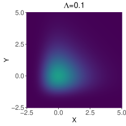
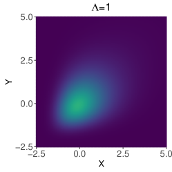
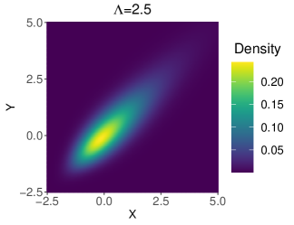
Figure 1: Densities of the bivariate Hüsler-Reiss distribution for different values of the dependence-related parameter $\Lambda$. A large (small) value of $\Lambda$ induces a strong (weak) dependence.

For $\Lambda=0.1,1$, and $2.5$, we present the PDFs of the BHR distribution in Figure 1. For these choices of $\Lambda$, the values of the $\chi$-measure are $1.52\times 10^{-23}$, 0.3173, and 0.6892, respectively. The figure demonstrates that a large (small) value of $\Lambda$ induces a strong (weak) dependence. Interchanging the arguments ($x$ and $y$), the PDF (7) remains the same; thus, the components of the BHR distribution are exchangeable.

3 Aviation Stock Price Dataset: Exploration and Pre-Processing

3.1 Data Description

This article focuses on analyzing the daily stock prices of two prominent Indian aviation companies, IndiGo and SpiceJet. We obtain the related datasets from the website https://www.investing.com/. We consider the period from December 2, 2019, to May 31, 2022, which coincides with the global COVID-19 pandemic. According to the World Health Organization (https://covid19.who.int/region/searo/country/in), India experienced three severe waves of the pandemic during this time. The first wave lasted from mid-March 2020 to mid-January 2021, followed by the deadliest second wave from mid-March 2021 to mid-August 2021. Lastly, the third wave persisted from mid-December 2021 to mid-March 2022. These waves had significant repercussions on various sectors of society and the economy, including the aviation market. Due to widespread travel restrictions and reduced investor activity, share prices experienced declines during the lockdown periods. This analysis aims to explore how the COVID-19 waves influenced the dependence between the share prices of these two aviation companies, with a focus on detecting the most crucial changepoint in their upper tail dependence, due to its link with simultaneous sell positions.

3.2 Maximum Return Rate

Instead of dealing with the stock prices in their original scales, we focus on analyzing their return rates, which are more meaningful comparison metrics. This rate signifies the percentage variation in the value of a particular stock investment over a specified period, indicating the level of gain or loss experienced by the investor on their stock holding. The return rate can be computed using the following formula:

$$\textrm{Return rate}\,=\,\frac{(\textrm{Ending price}\,-\,\textrm{Beginning price})\,+\,\textrm{Dividends}}{\textrm{Beginning price}}.$$

Here, the ending price corresponds to the stock price after a specified period, while the beginning price represents the stock price at the beginning of the same period. Additionally, the term “Dividends” refers to the total amount of dividends paid out by the company during that same period only. The return rate can take both positive and negative values, indicating whether an investor gains profit or incurs a loss on the investment, respectively. This measure holds great importance in evaluating the performance of a stock and comparing it to other investment options available. A standard period for calculating return rates is 24 hours and we stick to it here.

Given our focus on the right tail of the joint distribution of return rates, we define the daily maximum return rate as follows. Suppose $Y_{t}(s)$ represents the value of the stock on a specific day $t$ at time $s$. We calculate the daily maximum stock return rate $R_{t}$ on day $t$ by

$$R_{t} =\;\max_{s,s^{{}^{\prime}}}\;\left\{\frac{Y_{t+1}\,(s)\;-\;Y_{t}\,(s^{{}^{\prime}})}{Y_{t}\,(s^{{}^{\prime}})}\right\}=\;\frac{\max_{s}\,Y_{t+1}(s)}{\min_{s^{{}^{\prime}}}Y_{t}\,(s^{{}^{\prime}})}\,-\,1.$$ (8)

The standard publicly available datasets include both the daily maximum stock price $\max_{s}\,Y_{t+1}(s)$ and the daily minimum stock price $\min_{s^{{}^{\prime}}}Y_{t}\,(s^{{}^{\prime}})$. Hence, calculating $R_{t}$ from them is straightforward. The plots of daily maximum stock prices and $R_{t}$’s for both IndiGo and SpiceJet are presented in Figure 2. The daily maximum stock prices for both companies were low during the first wave of the COVID-19 period; however, the jumps (drops and hikes both) in the case of SpiceJet are sharper than those for IndiGo. After the first wave, the daily maximum stock prices show an increasing pattern for IndiGo, while an opposite pattern is observable for SpiceJet. The daily maximum return rate profiles are relatively more stable than the actual stock prices. However, we can observe a more jittery pattern for SpiceJet than IndiGo. During the initial days of the COVID-19 pandemic in India, $R_{t}$ profiles attend negative values for both airlines; however, the lowest value of $R_{t}$ is more negative for SpiceJet than that for IndiGo, and the subsequent $R_{t}$ values attend higher positive values for IndiGo than that for SpiceJet. A clear nonstationary pattern is observable in both series.

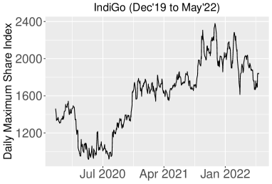
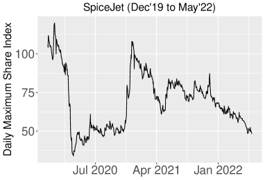
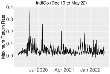
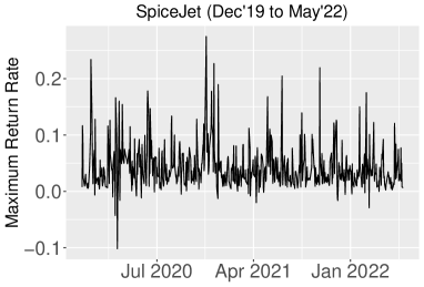
Figure 2: Daily maximum stock return of IndiGo and SpiceJet airlines (top panels) and the corresponding daily maximum return rates (bottom panels) as defined in (8).

3.3 Data Preprocessing

While the Fisher-Tippett theorem described in Section 2 assumes the underlying sequence of random variables to be independently and identically distributed, the result also holds in the case of dependent sequences under some additional regularity conditions explained in Leadbetter and Rootzen (1988). Here, the original stock prices across different timestamps $s$ on a certain day $t$, denoted by $Y_{t}(s)$ in (8), are likely to be dependent. Assuming the regularity conditions of Leadbetter and Rootzen (1988) hold, we assume that $R_{t}$’s follow the GEV distribution in (1), characterized by three parameters– location ($\mu$), scale ($\psi$), and shape ($\xi$). Therefore, to transform $R_{t}$’s to standard Gumbel margins, our first data preprocessing step involves estimating these parameters. However, the bottom panels of Figure 2 show that assuming the GEV parameters to be constant across $t$ is questionable for both airlines. Hence, we assume the marginal model to be $R_{t}\sim\textrm{GEV}(\mu_{t},\sigma_{t},\xi_{t})$ separately for each company. Here, we estimate the temporally-varying GEV parameters using local probability-weighted moments (PWM, Hosking et al., 1985) estimation.

In general, the term local likelihood, introduced by Tibshirani and Hastie (1987), refers to a method that estimates the parameters of a statistical model by considering local subsets of data instead of the entire dataset as a whole. The local likelihood approach involves placing a window around each observation and maximizing the likelihood function for the model’s parameters within that window. In our case, we utilize a window size of 100 for each analysis and employ PWM estimation. Unlike the traditional method of moments, where we equate population moments to their sample counterparts with equal weights, PWM utilizes a set of weights that depends on the probability density function of the population. These weights are carefully selected to capture the distribution’s shape more accurately, and thus, the PWM method is used widely in extreme value analysis. Implementing local PWM estimation, we obtain the estimates of $\{\mu_{t},\sigma_{t},\xi_{t}\}$ separately for IndiGo and SpiceJet at each day $t$ during the COVID-19 pandemic. We obtained the shape parameter estimates to be close to zero in almost all the cases, along with high standard errors. Thus, the shape parameter can be safely fixed to zero, i.e., the corresponding GEV distribution can be assumed to belong to the Gumbel class, for both airlines. We then apply the local PWM estimation procedure after setting $\xi_{t}=0$ for all cases.

Further, suppose we denote the joint daily maximum return rate vector for day $t$ by $\bm{R}_{t}=(R^{X}_{t},R^{Y}_{t})^{\prime}$, where $R^{X}_{t}$ and $R^{Y}_{t}$ denote the individual daily maximum return rates on day $t$ for IndiGo and SpiceJet, respectively. Besides, let the corresponding local PWM estimates for the parameters of the underlying Gumbel distributions be given by $\{\widehat{\mu}^{X}_{t},\widehat{\sigma}^{X}_{t}\}$ and $\{\widehat{\mu}^{Y}_{t},\widehat{\sigma}^{Y}_{t}\}$, respectively. We transform $R^{X}_{t}$ and $R^{Y}_{t}$ to standard Gumbel margins following the location-scale transformations

$$\widetilde{R}^{X}_{t}=\frac{R^{X}_{t}-\widehat{\mu}^{X}_{t}}{\widehat{\sigma}^{X}_{t}},\quad\widetilde{R}^{Y}_{t}=\frac{R^{Y}_{t}-\widehat{\mu}^{Y}_{t}}{\widehat{\sigma}^{Y}_{t}},$$ (9)

and obtain the transformed random vectors $\widetilde{\bm{R}}_{t}=(\widetilde{R}^{X}_{t},\widetilde{R}^{Y}_{t})$.

We explore the temporal extremal dependence within the time series $\{\widetilde{R}^{X}_{t}\}$ and $\{\widetilde{R}^{Y}_{t}\}$ through $F$-madogram as in (5). For both series, we observe that the estimated temporal $\chi$-measures are close to zero across low through high lags, and thus, we safely assume each of $\{\widetilde{R}^{X}_{t}\}$ and $\{\widetilde{R}^{Y}_{t}\}$ to be independent across $t$. To explore the extremal dependence between the components of $\widetilde{\bm{R}}_{t}$, we estimate it using $F$-madogram similar to its use for exploring temporal extremal dependence. We obtain the empirical $\chi$-measure to be 0.2553. Under the null hypothesis of independence between the components of $\widetilde{\bm{R}}_{t}$, the bootstrap-based critical value is 0.0646 based on a test of level 0.95. Thus, we can safely claim that there is a strong extremal dependence between the components of $\widetilde{\bm{R}}_{t}$, and further, we assume that the joint distribution of $\widetilde{\bm{R}}_{t}$ is the BHR distribution with CDF (6).

4 Methodology

In this section, we discuss the Likelihood Ratio Test (LRT) and Modified Information Criterion (MIC) to detect changepoints in the BHR distribution. Let the transformed daily maximum return rate vectors $\{\widetilde{\bm{R}}_{t}=(\widetilde{R}^{X}_{t},\widetilde{R}^{Y}_{t}),t=1,\ldots,T\}$ in (9) be a sequence of independent observations from the BHR distribution with dependence-related parameters $\{\Lambda_{t},t=1,\ldots,T\}$ respectively. We are interested in testing for changes in the parameters $\Lambda_{t}$’s, i.e., our null and alternative hypotheses of interest are

$$H_{0}\;:\;\Lambda_{1}=\cdots=\Lambda_{T}=\Lambda,\quad H_{A}\;:\;\Lambda_{1}=\ldots=\Lambda_{\tau}\neq\Lambda_{\tau+1}=\cdots=\;\Lambda_{T-1}\;=\;\Lambda_{T}$$

for a changepoint $\tau$, if exists. Then, under $H_{0}$, the log-likelihood is

$$\log L_{H_{0}}(\Lambda)=\sum_{t=1}^{T}\log\left[h_{\Lambda}\left(\widetilde{R}^{X}_{t},\widetilde{R}^{Y}_{t}\right)\right],$$ (10)

where $h_{\Lambda}(\cdot,\cdot)$ is as in (7), and the corresponding maximum likelihood estimate (MLE) of $\Lambda$, say $\widehat{\Lambda}$, is obtained by solving the following score equation

$$\frac{\partial}{\partial\Lambda}(\log\,L_{H_{0}}(\Lambda))=0.$$ (11)

Under the alternative hypothesis $H_{A}$, the log-likelihood function is

$$\log L_{H_{A}}(\Lambda_{1},\Lambda_{T},\tau)=\sum_{t=1}^{\tau}\log\left[h_{\Lambda_{1}}\left(\widetilde{R}^{X}_{t},\widetilde{R}^{Y}_{t}\right)\right]+\log\left[\sum_{t=\tau+1}^{T}h_{\Lambda_{T}}\left(\widetilde{R}^{X}_{t},\widetilde{R}^{Y}_{t}\right)\right],$$ (12)

and we obtain the MLEs of $\Lambda_{1}$ and $\Lambda_{T}$, say $\widehat{\Lambda}_{1}$ and $\widehat{\Lambda}_{T}$ respectively, by solving the following score equations

$$\frac{\partial}{\partial\Lambda_{1}}(\log\,L_{H_{A}}(\Lambda_{1},\Lambda_{T},\tau))=0,\quad\frac{\partial}{\partial\Lambda_{T}}(\log\,L_{H_{A}}(\Lambda_{1},\Lambda_{n},\tau))=0.$$ (13)

The above score equations (11) and (13) require nonlinear optimization and we use the function fbvevd from the R package evd (Stephenson, 2002) to get the MLEs.

4.1 Likelihood Ratio Test (LRT)

The most commonly used test for changepoint detection problems is LRT. Its asymptotic properties have been studied in detail in the literature and it provides theoretical guarantees under certain regularity conditions (Csörgö and Horváth, 1997).

LRT works in the following way. Consider a timepoint $\tau$ between $1$ and $T$ at which a change occurs. We reject our null hypothesis, i.e., no changepoint, if we observe a high value of the (2-times the log) likelihood ratio, for a fixed $\tau$, given by

$$\textrm{LR}(\tau) =-2\left\{\log L_{H_{0}}(\widehat{\Lambda})-\log L_{H_{A}}(\widehat{\Lambda}_{1},\widehat{\Lambda}_{T})\right\},$$ (14)

where $\log L_{H_{0}}$ and $\log L_{H_{A}}$ are given by (10) and (12), respectively. Further, considering a range of possible values of $\tau$, the alternative hypothesis is preferred if $\textrm{LR}(\tau)$ is high for any single $\tau$ and the related LRT statistic is given by

$$Z_{T}\;=\;\max_{1\leq\tau<T}\;\textrm{LR}(\tau).$$

If $\tau$ is small, we do have not sufficient data to obtain the MLE $\widehat{\Lambda}_{1}$. Similarly, for $\tau$ close to $T$, $\widehat{\Lambda}_{T}$ would be unstable due to insufficient data. Thus, to avoid high uncertainty of the estimates, Ngunkeng and Ning (2014) suggested the modified version of $Z_{T}$, or in other words the trimmed LRT statistic $Z^{\prime}_{T}$ given by

$$Z^{\prime}_{T}\;=\;\max_{\tau_{0}<\tau<T-\tau_{0}}\;\textrm{LR}(\tau),\;\;\textrm{where}\;\;\tau_{0}=2\lfloor\log(T)\rfloor.$$ (15)

while other choices of $\tau_{0}$ have been proposed in the literature, e.g., Liu and Qian (2009) suggested $\tau_{0}\;=\;\lfloor\log\,T\rfloor^{2}$, we stick to the choice in (15). Once we reject our null hypothesis, the estimated changepoint is

$$\widehat{\tau}_{\textrm{LRT}}\;=\;\operatorname*{arg\,max}_{\tau_{0}<\tau<T-\tau_{0}}\;\textrm{LR}(\tau).$$ (16)

For a given level of significance $\alpha$, we reject our null hypothesis $H_{0}$ if $Z^{\prime}_{T}>c_{\alpha,\;T}$, where $c_{\alpha,\;T}$ is the corresponding critical value. In Section 5, we numerically obtain $c_{\alpha,\;T}$ for different choices of $T$ and $\alpha$, and different true values of the dependence-related parameter $\Lambda$.

4.2 Modified Information Criterion (MIC)

The Modified Information Criterion (MIC) was proposed by Chen et al. (2006). The authors also showed that MIC has simple asymptotic behaviors and is consistent in selecting the correct model. Said et al. (2019) pointed out that MIC performs better than LRT in detecting the changepoints occurring near the very beginning or at the very end of the data sequence.

The idea of MIC is as follows. Similar to the case of LRT, consider an integer $\tau$ between $1$ (included) to $T$. If a change occurs at any $\tau$, we reject our null hypothesis $H_{0}$, i.e., no changepoint. Under $H_{0}$, we have $\tau=T$, and then, the MIC is defined as

$$\textrm{MIC}(T)\;=\;-2\log L_{H_{0}}(\widehat{\Lambda})\;+\;dim(\Lambda)\log(T),$$

where $\widehat{\Lambda}$ is the solution of (11). For the BHR distribution, the dimension of the parameter space is dim($\Lambda$) = 1. For $1\leq\,\tau<T$, the MIC is defined as

$$\textrm{MIC}(\tau)\;=\;-2\log L_{H_{A}}(\widehat{\Lambda}_{1},\;\widehat{\Lambda}_{T})\;+\;\left[2\;\textrm{dim}(\Lambda_{1})\;+\;\left(\frac{2\tau}{T}-1\right)^{2}\right]\log(T);$$ (17)

here, for our model, $\textrm{dim}(\Lambda_{1})=1$. If $\textrm{MIC}(T)\geq\min_{1\leq\tau<T}\textrm{MIC}(\tau)$, we select the model with a changepoint. Then, the estimated changepoint $\widehat{\tau}$ satisfies the equality $\textrm{MIC}(\widehat{\tau})=\min_{1\leq\tau<T}\textrm{MIC}(\tau)$. Chen et al. (2006) also suggested a test statistics $S_{T}$ based on $\textrm{MIC}(T)$ and $\textrm{MIC}(\tau)$ to detect one changepoint as follows

$$S_{T}=\textrm{MIC}(T)\;-\;\min_{1\leq\tau<T}\;\textrm{MIC}(\tau)\;+\;dim(\Lambda)\log(T).$$

For our model, dim$(\Lambda)$ = 1, and hence, $S_{T}$ can be written for our case as

$$S_{T}=-2\log L_{H_{0}}(\widehat{\Lambda})-\min_{1\leq\tau<T}\left[-2\log L_{H_{A}}(\widehat{\Lambda}_{1},\widehat{\Lambda}_{T})+\left\{\left(\frac{2\tau}{T}-1\right)^{2}-1\right\}\log(T)\right].$$

If changepoints occur at the very beginning or the end, then we do have not sufficient data to obtain the MLEs $\widehat{\Lambda}_{1}$ or $\widehat{\Lambda}_{T}$. In these cases, Ngunkeng and Ning (2014) suggested a trimmed version of $S_{T}$ as

$$S^{\prime}_{T}=-2\log L_{H_{0}}(\widehat{\Lambda})-\min_{\tau_{0}<\tau<T-\tau_{0}}\left[-2\log L_{H_{A}}(\widehat{\Lambda}_{1},\widehat{\Lambda}_{T})+\left\{\left(\frac{2\tau}{T}-1\right)^{2}-1\right\}\log(T)\right].$$ (18)

where $\tau_{0}=2\lfloor\log(T)\rfloor$. Applications of $S^{\prime}_{T}$ can be found in Tian and Yang (2022). Once we reject our null hypothesis, the estimated changepoint is

$$\widehat{\tau}_{\textrm{MIC}}\;=\;\operatorname*{arg\,min}_{\tau_{0}<\tau<T-\tau_{0}}\;\textrm{MIC}(\tau).$$ (19)

We reject our null hypothesis if $S^{\prime}_{T}>c_{\alpha,\;T}$, where $c_{\alpha,\;T}$ is the critical value for a given level of significance $\alpha$. We numerically obtain $c_{\alpha,\;T}$ for different choices of $T$, $\alpha$, and true dependence-related parameter $\Lambda$, and we tabulate them in Section 5.

5 Simulation Study

Here we discuss obtaining critical values for the LRT statistic $Z^{\prime}_{T}$ in (15) and the MIC statistic $S^{\prime}_{T}$ in (18) and compare their performances in terms of power. We derive the critical values and power numerically due to their intractable analytic expressions.

5.1 Critical Values

We numerically evaluate the critical values $c_{\alpha,T}$ for a few specific choices of the true parameter values $\Lambda$ of the BHR distribution, levels of significance $\alpha$, and sample sizes $T$, to illustrate the procedure for obtaining the critical values under a general set-up as well as for studying their patterns. We consider three choices of $\Lambda\in\{0.5,2,4\}$ under the null distribution, four choices of $T\in\{50,100,150,200\}$, and $\alpha\in\{0.01,0.05,0.1\}$.

For a choice of the true value of $\Lambda$ and $T$, we first obtain $B=10^{4}$ samples each comprising of $T$ IID observations from the BHR distribution with dependence-related parameter $\Lambda$, say $\mathcal{R}^{(b)}=\{\widetilde{\bm{R}}^{(b)}_{1},\ldots,\widetilde{\bm{R}}^{(b)}_{T}\}$ for $b=1,\ldots,B$. Then, we obtain $\widehat{\Lambda}^{(b)}$, the MLE of $\Lambda$ based on $\mathcal{R}^{(b)}$, following (11), and then calculate $\log L_{H_{0}}(\widehat{\Lambda}^{(b)})$ based on $\mathcal{R}^{(b)}$, following (10). Further, for each $\tau$ between $\tau_{0}=2\lfloor\log(T)\rfloor$ and $T-\tau_{0}$ (excluding the endpoints), we divide the sample $\mathcal{R}^{(b)}$ into two parts $\mathcal{R}^{(b,1)}=\{\widetilde{\bm{R}}^{(b)}_{1},\ldots,\widetilde{\bm{R}}_{\tau}^{(b)}\}$ and $\mathcal{R}^{(b,T)}=\{\widetilde{\bm{R}}_{\tau+1}^{(b)},\ldots,\widetilde{\bm{R}}^{(b)}_{T}\}$. We then assume that the observations in $\mathcal{R}^{(b,1)}$ and $\mathcal{R}^{(b,T)}$ follow two different BHR distributions with parameters $\Lambda_{1}$ and $\Lambda_{T}$, respectively, and obtain the MLEs $\widehat{\Lambda}^{(b)}_{1}$ and $\widehat{\Lambda}^{(b)}_{T}$ following (13). Based on $\mathcal{R}^{(b,1)}$, $\mathcal{R}^{(b,T)}$, $\widehat{\Lambda}^{(b)}_{1}$, and $\widehat{\Lambda}^{(b)}_{T}$, we calculate $\log L_{H_{A}}(\widehat{\Lambda}^{(b)}_{1},\widehat{\Lambda}^{(b)}_{T})$ following (12). We repeat the above procedure for each $\tau_{0}<\tau<T-\tau_{0}$ and calculate $Z^{\prime}_{T}$ following (15); we call it $Z^{{}^{\prime}(b)}_{T}$. We repeat the whole procedure for each $b=1,\ldots,B$ and obtain $\mathcal{Z}_{T}=\{Z^{{}^{\prime}(1)}_{T},\ldots,Z^{{}^{\prime}(B)}_{T}\}$. Similar to LRT statistics, based on $\log L_{H_{0}}(\widehat{\Lambda}^{(b)})$ and $\log L_{H_{A}}(\widehat{\Lambda}^{(b)}_{1},\widehat{\Lambda}^{(b)}_{T})$ for all $\tau_{0}<\tau<T-\tau_{0}$, we calculate $S^{\prime}_{T}$ following (18); we call it $S^{{}^{\prime}(b)}_{T}$. We repeat the whole procedure for each $b=1,\ldots,B$ and obtain $\mathcal{S}_{T}=\{S^{{}^{\prime}(1)}_{T},\ldots,S^{{}^{\prime}(B)}_{T}\}$. Finally, the critical values $c_{\alpha,T}$ for LRT and MIC are obtained by the $100(1-\alpha)$-th percentiles of $\mathcal{Z}_{T}$ and $\mathcal{S}_{T}$, respectively. Due to the inherent randomness of the above-explained sampling-based procedure, we also calculate the standard error of $c_{\alpha,T}$ for LRT and MIC using a straightforward nonparametric bootstrap procedure from $\mathcal{Z}_{T}$ and $\mathcal{S}_{T}$, as otherwise repeating the parametric bootstrap procedure several times would be computationally challenging. The critical values for both LRT and MIC and their (Monte Carlo) standard errors (S.E.) are presented in Table 1. For smaller $\alpha$, $c_{\alpha,T}$ are naturally higher. For a specific $\Lambda$ and $\alpha$, $c_{\alpha,T}$ are generally higher as $T$ increases; however, the underlying high S.E.s indicate that such differences are generally insignificant. The S.E.s of $c_{\alpha,T}$ are high for small $\alpha$ for all $\Lambda$ and $T$ for both LRT and MIC. By construction, the $c_{\alpha,T}$ values are smaller for MIC than that for LRT for any $\Lambda$, $T$, and $\alpha$.

Table 1: Critical values of LRT and MIC for different levels of significance $\alpha$ and different sample sizes $T$.

LRT
$T$	$\Lambda$		$\alpha\,=\,0.01$	$\alpha\,=\,0.05$	$\alpha\,=\,0.1$	$T$	$\Lambda$		$\alpha\,=\,0.01$	$\alpha\,=\,0.05$	$\alpha\,=\,0.1$
50	0.5	Cutoff	7.917	4.532	3.285	100	0.5	Cutoff	7.996	4.860	3.535
		S.E.	0.216	0.084	0.049			S.E.	0.236	0.084	0.052
	2	Cutoff	8.737	5.617	4.335		2	Cutoff	9.529	5.978	4.545
		S.E.	0.226	0.085	0.062			S.E.	0.177	0.097	0.078
	4	Cutoff	8.580	5.589	4.238		4	Cutoff	9.225	5.976	4.612
		S.E.	0.181	0.085	0.059			S.E.	0.231	0.089	0.053
150	0.5	Cutoff	7.966	4.948	3.654	200	0.5	Cutoff	8.036	4.968	3.698
		S.E.	0.185	0.086	0.053			S.E.	0.210	0.087	0.055
	2	Cutoff	9.405	6.178	4.738		2	Cutoff	9.676	6.155	4.807
		S.E.	0.278	0.087	0.069			S.E.	0.207	0.087	0.059
	4	Cutoff	9.369	6.112	4.692		4	Cutoff	9.588	6.263	4.786
		S.E.	0.171	0.095	0.067			S.E.	0.238	0.092	0.079
MIC
$T$	$\Lambda$		$\alpha\,=\,0.01$	$\alpha\,=\,0.05$	$\alpha\,=\,0.1$	$T$	$\Lambda$		$\alpha\,=\,0.01$	$\alpha\,=\,0.05$	$\alpha\,=\,0.1$
50	0.5	Cutoff	6.723	3.553	2.406	100	0.5	Cutoff	6.181	3.392	2.238
		S.E.	0.236	0.081	0.052			S.E.	0.191	0.099	0.044
	2	Cutoff	7.510	4.540	3.292		2	Cutoff	7.600	4.200	2.957
		S.E.	0.213	0.087	0.056			S.E.	0.257	0.082	0.053
	4	Cutoff	7.385	4.559	3.273		4	Cutoff	7.434	4.161	2.953
		S.E.	0.165	0.081	0.051			S.E.	0.167	0.061	0.056
150	0.5	Cutoff	6.016	3.271	2.179	200	0.5	Cutoff	5.440	3.008	2.017
		S.E.	0.193	0.064	0.045			S.E.	0.205	0.068	0.039
	2	Cutoff	6.896	3.981	2.806		2	Cutoff	7.031	3.747	2.508
		S.E.	0.252	0.073	0.051			S.E.	0.249	0.079	0.052
	4	Cutoff	7.164	4.029	2.749		4	Cutoff	6.778	3.743	2.535
		S.E.	0.200	0.083	0.060			S.E.	0.228	0.069	0.054

5.2 Power Comparison

In this subsection, we compare the power of LRT and MIC numerically under different scenarios of the alternative hypothesis $H_{A}$, i.e., we fix the changepoint $\tau$, the values of the dependence-related parameter of the BHR distribution before and after the changepoint, i.e., $\Lambda_{1}$ and $\Lambda_{T}$. We choose the sample sizes $T\in\{50,200\}$ and the levels of significance $\alpha\in\{0.01,0.05,0.1\}$. Then, for each $T$, we choose two different values of the changepoint $\tau=\lfloor\beta T\rfloor$, where $\beta\in\{0.25,0.5\}$. In each case, we consider the possible values of the dependence-related parameter before and after the changepoint as $\Lambda_{1}\in\{0.5,2,4\}$ and $\Lambda_{T}\in\{0.5,1,1.5,\ldots,5\}$, respectively. Under $H_{0}$, $\tau=T$ and the value of the dependence-related parameter under $H_{0}$ is the same as $\Lambda_{1}$. Hence, for the above choices, the critical values of LRT and MIC are obtained as in Section 5.1.

For a choice of the true values of $\Lambda_{1}$, $\Lambda_{T}$, $\tau$, and $T$, we first obtain $B=10^{4}$ samples each comprising of $\tau$ IID observations from the BHR distribution with dependence-related parameter $\Lambda_{1}$, say $\mathcal{R}^{(b,1)}=\{\widetilde{\bm{R}}^{(b)}_{1},\ldots,\widetilde{\bm{R}}_{\tau}^{(b)}\}$ and another $T-\tau$ IID observations from the BHR distribution with parameter $\Lambda_{T}$, say $\mathcal{R}^{(b,T)}=\{\widetilde{\bm{R}}_{\tau+1}^{(b)},\ldots,\widetilde{\bm{R}}^{(b)}_{T}\}$, for $b=1,\ldots,B$. For each $b$, we thus obtain a combined sample of size $T$ given by $\mathcal{R}^{(b)}=\{\widetilde{\bm{R}}^{(b)}_{1},\ldots,\widetilde{\bm{R}}^{(b)}_{T}\}$. Under $H_{0}$, we assume the observations in $\mathcal{R}^{(b)}$ to be IID following a BHR distribution with a common parameter $\Lambda$. Following (11), we obtain the MLE of $\Lambda$ given by $\widehat{\Lambda}^{(b)}$ and then calculate $\log L_{H_{0}}(\widehat{\Lambda}^{(b)})$ based on $\mathcal{R}^{(b)}$, following (10). Subsequently, under $H_{A}$, we obtain the MLEs $\widehat{\Lambda}^{(b)}_{1}$ and $\widehat{\Lambda}^{(b)}_{T}$ following (13). Based on $\mathcal{R}^{(b,1)}$, $\mathcal{R}^{(b,T)}$, $\widehat{\Lambda}^{(b)}_{1}$, and $\widehat{\Lambda}^{(b)}_{T}$, we calculate $\log L_{H_{A}}(\widehat{\Lambda}^{(b)}_{1},\widehat{\Lambda}^{(b)}_{T})$ following (12). We repeat the above procedure for each $\tau_{0}<\tau<T-\tau_{0}$ and calculate $Z^{\prime}_{T}$ following (15); we call it $Z^{{}^{\prime}(b)}_{T}$. We repeat the whole procedure for each $b=1,\ldots,B$ and obtain $\mathcal{Z}_{T}=\{Z^{{}^{\prime}(1)}_{T},\ldots,Z^{{}^{\prime}(B)}_{T}\}$. Similar to LRT statistics, based on $\log L_{H_{0}}(\widehat{\Lambda}^{(b)})$ and $\log L_{H_{A}}(\widehat{\Lambda}^{(b)}_{1},\widehat{\Lambda}^{(b)}_{T})$ for all $\tau_{0}<\tau<T-\tau_{0}$, we calculate $S^{\prime}_{T}$ following (18); we call it $S^{{}^{\prime}(b)}_{T}$. We repeat the whole procedure for each $b=1,\ldots,B$ and obtain $\mathcal{S}_{T}=\{S^{{}^{\prime}(1)}_{T},\ldots,S^{{}^{\prime}(B)}_{T}\}$. The reader should note that despite having a true value of $\tau$ under $H_{A}$, both LRT and MIC should be calculated based on maximizing the necessary terms in (15) and (18) over $\tau_{0}<\tau<T-\tau_{0}$. The critical values are obtained apriori following Section 5.1 and suppose we call the critical values $c_{\alpha,T}$ for LRT and MIC by $c^{\textrm{LRT}}_{\alpha,T}$ and $c^{\textrm{MIC}}_{\alpha,T}$, respectively. We thus can approximate their powers by

$$P_{\textrm{LRT}}=\frac{1}{B}\sum_{b=1}^{B}\textrm{I}\left(Z_{T}^{{}^{\prime}{(b)}}\geq c^{\textrm{LRT}}_{\alpha,T}\right),\quad P_{\textrm{MIC}}=\frac{1}{B}\sum_{b=1}^{B}\textrm{I}\left(S_{T}^{{}^{\prime}(b)}\geq c^{\textrm{MIC}}_{\alpha,T}\right),$$ (20)

where I($\cdot$) is an indicator function.

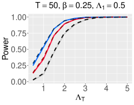
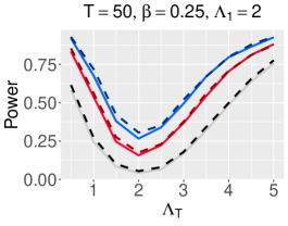
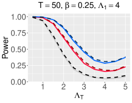
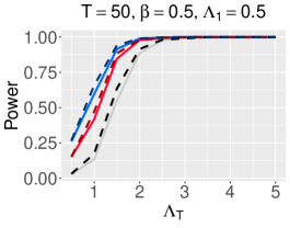
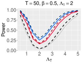
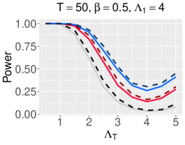
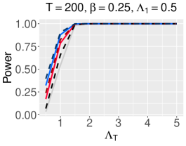
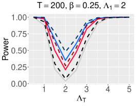
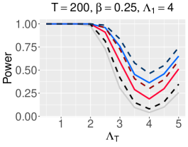
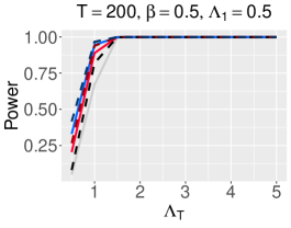
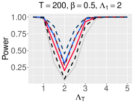
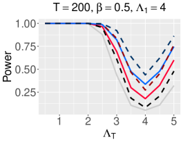
Figure 3: Power curves of LRT and MIC under different choices of $T$, $\tau=\lfloor\beta T\rfloor$, $\Lambda_{1}$, $\Lambda_{T}$, and $\alpha$. The curves for LRT are presented by solid lines while the curves for MIC are presented by dashed lines. For each case, the curves from bottom to top, represented in black, red, and blue, are for $\alpha=0.01,0.05,0.1$, respectively. A higher value of power indicates a better testing procedure.

We present the power curves in Figure 3. For both LRT and MIC, the power is higher for larger levels of significance $\alpha$ under all settings; this is obvious and follows directly from (20). When $T=50$, $\beta=0.25$, and $\Lambda_{1}=0.5$, the power curves of LRT and MIC for $\alpha=0.01$ are close to one only when $\Lambda_{T}\approx 3.5$. After changing $\beta=0.25$ to $\beta=0.5$ keeping other parameters fixed, both power curves for $\alpha=0.01$ are close to one when $\Lambda_{T}\approx 2.5$. Here, the availability of more observations for estimating $\Lambda_{1}$ allows higher power even when the difference between $\Lambda_{1}$ and $\Lambda_{T}$ remains the same. In general, the power of both LRT and MIC are higher for $\beta=0.5$ than for $\beta=0.25$ while keeping the other parameters fixed. This feature is more prominent when the sample size is small. Keeping other parameters fixed (with respect to the top-left panel), increasing the sample size from $T=50$ to $T=200$, the power increases significantly for both tests; both power curves for $\alpha=0.01$ are close to one when $\Lambda_{T}\approx 1.5$. A similar increasing pattern in power curves is visible for other values of $\Lambda_{1}$ and $\beta$. In all cases, naturally, the power is lowest when $\Lambda_{1}=\Lambda_{T}$. For $T=50$ and $\Lambda_{1}=2$, we observe that the power curves are asymmetric for $\Lambda_{T}<\Lambda_{1}$ and $\Lambda_{T}>\Lambda_{1}$. When $\Lambda_{T}<\Lambda_{1}$, the power values of LRT and MIC get closer to one faster than that in the case of $\Lambda_{T}>\Lambda_{1}$. For $T=200$, the power curves become more symmetric around $\Lambda_{1}$. However, for this asymmetry changes with the value of $\Lambda_{1}$; for example, when $\Lambda_{1}=0.5$ and $T=200$, the power curves reach near one when $\Lambda_{T}-\Lambda_{1}\approx 1$, while for $\Lambda_{1}=4$ and $T=200$, all the power curves become close to one only when $\Lambda_{1}-\Lambda_{T}\approx 2$. In general, MIC appears to be more powerful than LRT. This characteristic is more prominent when $T=200$. For both $T=50$ and $T=200$, the differences between the power curves of LRT and MIC are generally more prominent when $\beta=0.5$ compared to the case of $\beta=0.25$.

5.3 Consistency of the Estimator of Changepoint

There is a vast literature on the asymptotic theoretical guarantees of both LRT (Csörgö and Horváth, 1997) and MIC (Chen et al., 2006). They hold in general under certain regularity conditions. However, despite the availability of asymptotic results, an analytical exposition of finite sample properties is often intricate because of the non-existence of any closed-form expression of the estimators of changepoint $\widehat{\tau}_{\textrm{LRT}}$ in (16) and $\widehat{\tau}_{\textrm{MIC}}$ in (19). As a result, in this subsection, we numerically calculate the probabilities of the estimators $\widehat{\tau}_{\textrm{LRT}}$ and $\widehat{\tau}_{\textrm{MIC}}$ being within a small neighborhood of the true value of the changepoint $\tau$, i.e., $\textrm{P}(|\widehat{\tau}-\tau|\leq\delta)$ for $\widehat{\tau}=\widehat{\tau}_{\textrm{LRT}},\widehat{\tau}_{\textrm{MIC}}$ and $\delta=1,2,3$. We calculate this probability under different scenarios of the alternative hypothesis $H_{A}$, i.e., we fix the changepoint $\tau$, the values of the dependence-related parameter of the BHR distribution before and after the changepoint, i.e., $\Lambda_{1}$ and $\Lambda_{T}$. We choose the sample sizes $T\in\{50,200\}$. Then, for each $T$, we choose two different values of the changepoint $\tau=\lfloor\beta T\rfloor$, where $\beta\in\{0.25,0.5\}$. In each case, we consider the possible values of the dependence-related parameter before and after the changepoint as $\Lambda_{1}\in\{0.5,1,1.5,\ldots,5\}$ and $\Lambda_{T}\in\{0.5,2,4\}$, respectively. We ignore the cases when $\Lambda_{1}=\Lambda_{T}$ as they indicate no changepoint scenarios.

We present the curves of $\textrm{P}(|\widehat{\tau}-\tau|\leq\delta)$ in Figure 4. As $\delta$ increases, $\textrm{P}(|\widehat{\tau}-\tau|\leq\delta)$ naturally also increases for $\widehat{\tau}=\widehat{\tau}_{\textrm{LRT}},\widehat{\tau}_{\textrm{MIC}}$ under all settings. When $T=50,\beta=0.25$, and $\Lambda_{T}=0.5$ (top-left panel), the values of $\textrm{P}(|\widehat{\tau}-\tau|\leq\delta)$ are close to each other for LRT and MIC; for small differences between $\Lambda_{1}$ and $\lambda_{T}$, LRT performs slightly better than MIC and the difference fades away as the difference between $\Lambda_{1}$ and $\lambda_{T}$ increases. Upon changing $\Lambda_{T}=0.5$ to $\Lambda_{T}=2$, the difference in $\textrm{P}(|\widehat{\tau}-\tau|\leq\delta)$ between LRT and MIC is more prominent, and LRT generally outperforms MIC. Further, changing $\Lambda_{T}=2$ to $\Lambda_{T}=4$, we see a less prominent difference in performance between LRT and MIC. When $\beta=0.5$ (second row of Figure 4) instead of $\beta=0.25$ as in the previous cases, we notice an opposite pattern in terms of the performances of LRT and MIC, i.e., MIC performs better than LRT for small differences between $\Lambda_{1}$ and $\Lambda_{T}$, and for large values of $|\Lambda_{1}-\Lambda_{T}|$, both methods perform similarly. When $T=200$, both LRT and MIC perform equally in general, and for $\beta=0.5$, MIC outperforms LRT for small values of $|\Lambda_{1}-\Lambda_{T}|$. Theoretically, the probability $\textrm{P}(|\widehat{\tau}-\tau|\leq\delta)$ should converge to one as $T\uparrow\infty$ for any positive $|\Lambda_{1}-\Lambda_{T}|$; however, we see that for $|\Lambda_{1}-\Lambda_{T}|=0.5$, the probability is less than 0.5 for all settings we consider. However, corresponding to the bottom-left panel of Figure 4, for example, we observe that the inclusion probability is close to one for $\delta=3$ when $|\Lambda_{1}-\Lambda_{T}|=4.5$. This observation indicates that the convergence underlying the asymptotic consistency holds only slowly while increasing $T$, and the difference in $\Lambda_{1}$ and $\Lambda_{T}$ plays a crucial role here.

We further study (not shown) the bias and mean squared error (MSE) in estimating the changepoint $\tau$ using $\widehat{\tau}_{\textrm{LRT}}$ and $\widehat{\tau}_{\textrm{MIC}}$. We observe that MIC produces significantly smaller values of MSE than LRT, and the difference is more prominent when $T=200$ compared to the case of $T=50$. Both bias and MSE are higher when the difference between $\Lambda_{1}$ and $\Lambda_{T}$ is small. We observe that the MSE decreases at a faster rate with $|\Lambda_{1}-\Lambda_{T}|$ when $\Lambda_{1}<\Lambda_{T}$ compared to the case when $\Lambda_{1}>\Lambda_{T}$. This pattern is consistent across the choices of $\beta$. For $\beta=0.25$, we observe positive biases for both LRT and MIC across all choices of $\Lambda_{1}$ and $\Lambda_{T}$. However, for $\beta=0.5$, we observe positive biases when $\Lambda_{1}>\Lambda_{T}$ and negative biases when $\Lambda_{1}<\Lambda_{T}$, irrespective of the method and the value of $T$. The absolute bias based on MIC is slightly higher than that for LRT when $\beta=0.25$, and the reverse is observable when $\beta=0.5$.

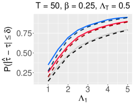
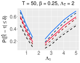
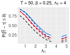
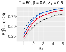
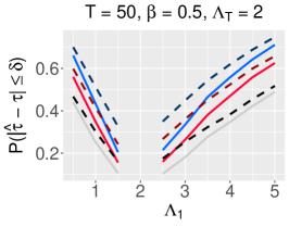
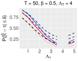
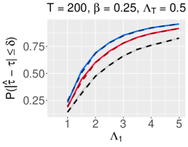
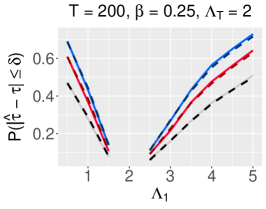
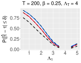
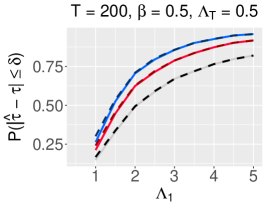
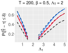
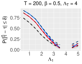
Figure 4: The probabilities $\textrm{P}(|\widehat{\tau}-\tau|\leq\delta)$ for $\widehat{\tau}=\widehat{\tau}_{\textrm{LRT}},\widehat{\tau}_{\textrm{MIC}}$ and $\delta\in\{1,2,3\}$ under different choices of $T$, $\tau=\lfloor\beta T\rfloor$, $\Lambda_{1}$, and $\Lambda_{T}$. The curves for LRT are presented by solid lines while the curves for MIC are presented by dashed lines. For each case, the curves from bottom to top, represented in black, red, and blue, are for $\delta=1,2,$ and 3, respectively. A higher value of $\textrm{P}(|\widehat{\tau}-\tau|\leq\delta)$ indicates a better accuracy in the estimation of a changepoint.

6 Data Application

6.1 Local Probability Weighted Moments Estimation

In Figure 2, we observe the nonstationary nature of the daily maximum return rates for both IndiGo and SpiceJet airlines, and in Section 3.3, we discuss considering the temporally-varying location and scale parameters of the underlying Gumbel distributions. We estimate them using local probability weighted moments estimation and obtain $\{\widehat{\mu}^{X}_{t},\widehat{\sigma}^{X}_{t}\}$, the location and scale parameters for IndiGo, and $\{\widehat{\mu}^{Y}_{t},\widehat{\sigma}^{Y}_{t}\}$, the location and scale parameters for SpiceJet, respectively. We present the time series of those estimates in Figure 5. The estimated location and scale profiles are higher during the first half of the COVID-19 period and lower during the second half for both airlines. This observation indicates that the median daily maximum return rates and variability are higher during the first half of the observation period, i.e., the overall volatility is high. Later, the median daily maximum return rates and the variability drop. All profiles attain peaks during August 2020; however, we observe a decreasing trend afterward for both profiles of SpiceJet, while the profiles stabilize afterward for IndiGo. This pattern indicates that the median daily maximum return rates are unstable after a volatile first half of the COVID-19 period. Both the estimated location profiles $\{\widehat{\mu}^{X}_{t},\widehat{\mu}^{Y}_{t}\}$ remain positive throughout the COVID-19 period. While our main focus in this paper and the next subsection is on the shifts in the dependence structure, the patterns observable in Figure 5 shed light on the marginal behavior of the daily maximum return rates.

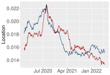
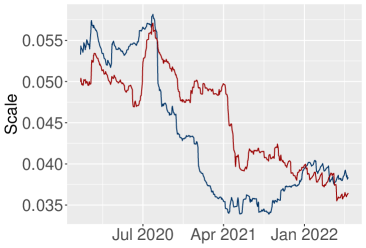
Figure 5: Local Probability Weighted Moments estimates of the temporally-varying location (left) and scale (right) parameters of the fitted Gumbel distribution to daily maximum return rates for IndiGo (blue) and SpiceJet (red) airlines.

6.2 Changepoint Estimation

Based on the estimated location and scale parameters of the marginal Gumbel distributions in Section 6.1, we transform the daily maximum return rates to standard Gumbel margins according to (9). We denote the transformed data by $\mathcal{R}=\{\widetilde{\bm{R}}_{t}=(\widetilde{R}^{X}_{t},\widetilde{R}^{Y}_{t}),t=1,\ldots,T\}$. We first calculate the LRT and MIC statistics as follows. Under $H_{0}$, we assume the observations in $\mathcal{R}$ to be IID following a BHR distribution with a common parameter $\Lambda$. Following (11), we obtain the MLE of $\Lambda$ given by $\widehat{\Lambda}$ and then calculate $\log L_{H_{0}}(\widehat{\Lambda})$ based on $\mathcal{R}$, following (10). Subsequently, under $H_{A}$, for each possible value of the changepoint $\tau$ such that $\tau_{0}<\tau<T-\tau_{0}$ where $\tau_{0}=2\lfloor\log(T)\rfloor$, we obtain the MLEs $\widehat{\Lambda}_{1}$ and $\widehat{\Lambda}_{T}$ following (13), based on $\mathcal{R}^{(1)}=\{\widetilde{\bm{R}}_{t},t=1,\ldots,\tau\}$ and $\mathcal{R}^{(T)}=\{\widetilde{\bm{R}}_{t},t=\tau+1,\ldots,T\}$, respectively. Based on $\mathcal{R}^{(1)}$, $\mathcal{R}^{(T)}$, $\widehat{\Lambda}_{1}$, and $\widehat{\Lambda}_{T}$, we calculate $\log L_{H_{A}}(\widehat{\Lambda}_{1},\widehat{\Lambda}_{T})$ following (12). Accordingly, we calculate $Z^{\prime}_{T}$ following (15); we call it $Z^{{}^{\prime}(obs)}_{T}$. Similarly, we calculate $S^{\prime}_{T}$ following (18); we call it $S^{{}^{\prime}(obs)}_{T}$.

Here, we deal with a real dataset, and thus, the true parameter values of the underlying distribution are unknown. Hence, for determining the critical values for both tests and the corresponding $p$-values, we use parametric bootstrapping. For each $b=1,\ldots,B$, where we choose $B=2000$, we draw an IID sample of size $T$, say $\mathcal{R}^{(b)}$, from the BHR distribution with parameter $\widehat{\Lambda}$. We repeat the same procedure of obtaining $Z^{\prime}_{T}$ and $S^{\prime}_{T}$ based on $\mathcal{R}^{(b)}$ and suppose we call them by $Z^{{}^{\prime}(b)}_{T}$ and $S^{{}^{\prime}(b)}_{T}$, respectively. We repeat the whole procedure for each $b=1,\ldots,B$ and obtain $\mathcal{Z}_{T}=\{Z^{{}^{\prime}(1)}_{T},\ldots,Z^{{}^{\prime}(B)}_{T}\}$ and $\mathcal{S}_{T}=\{S^{{}^{\prime}(1)}_{T},\ldots,S^{{}^{\prime}(B)}_{T}\}$. We calculate the critical values based on the $100(1-\alpha)$-th percentiles of $\mathcal{Z}_{T}$ and $\mathcal{S}_{T}$, respectively. The corresponding $p$-values are obtained by

$$p_{\textrm{LRT}}=\frac{1}{B}\sum_{b=1}^{B}\textrm{I}\left(Z_{T}^{{}^{\prime}{(b)}}\geq Z^{{}^{\prime}(obs)}_{T}\right),\quad p_{\textrm{MIC}}=\frac{1}{B}\sum_{b=1}^{B}\textrm{I}\left(S_{T}^{{}^{\prime}(b)}\geq S^{{}^{\prime}(obs)}_{T}\right).$$ (21)

In the case of LRT, we obtain a $p$-value of 0.027. Hence, we reject our null hypothesis $H_{0}$, i.e., no changepoint. We obtain the estimated changepoint to be $\widehat{\tau}_{\textrm{LRT}}=81$, which corresponds to the date March 26, 2020. Based on MIC, we obtain a $p$-value of 0.021. Hence, we also reject our null hypothesis $H_{0}$ based on MIC. We obtain the estimated changepoint to be $\widehat{\tau}_{\textrm{MIC}}=81$, which coincides with the result based on LRT. Figure 6 presents the profiles $\textrm{LR}(\tau)$ in (14) and $\textrm{MIC}(\tau)$ in (17). Apart from $\widehat{\tau}_{\textrm{LRT}}=\widehat{\tau}_{\textrm{MIC}}=81$, certain other peaks are also observable in both profiles $\textrm{LR}(\tau)$ and $\textrm{MIC}(\tau)$; the most prominent peaks, where $\textrm{LR}(\tau)$ is higher than 6, occur between $\tau=81$ and $\tau=94$. Corresponding to $\tau=81$, the MLE of $\Lambda_{1}$ and $\Lambda_{T}$ are $\widehat{\Lambda}_{1}=1.012$ and $\widehat{\Lambda}_{T}=1.540$, respectively. Ignoring the first and the last 50 days (due to the instability in estimation), for $\tau=81$, $\widehat{\Lambda}_{T}-\widehat{\Lambda}_{1}$ attains its highest value, which shows the correctness of the inference based on LRT and MIC.

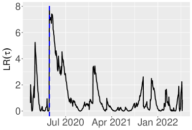
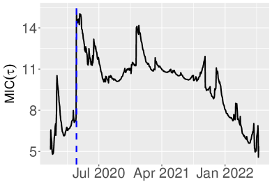
Figure 6: Temporal profiles of $\textrm{LR}(\tau)$ in (14) and $\textrm{MIC}(\tau)$ in (17).

According to Jaiswal (2020), the Government of India imposed a countrywide lockdown on March 25, 2020, which is very close to our estimated changepoint on March 26, 2020. This lockdown phase continued for 21 days, and all the high peaks in $\textrm{LR}(\tau)$ indicate this period. Before this date, we see less dependence (small $\Lambda_{1}$) between the daily maximum return rates of IndiGo and SpiceJet airlines due to the pre-lockdown situation. After the announcement of the lockdown, the aviation sector faced an unprecedented interruption, and both return rates behaved in a more similar fashion; this led to a higher $\Lambda_{T}$ than $\Lambda_{1}$. Despite the two companies focusing on different strategies to mitigate the challenges posed by COVID-19 as described in Section 1, the effect of the initial phase of the lockdown appears to be the strongest one.

7 Discussions and Conclusions

The literature on changepoint estimation in the context of extreme value analysis is scarce. Some recent publications (Jarušková and Rencová, 2008; Dierckx and Teugels, 2010; do Nascimento and e Silva, 2017; Lattanzi and Leonelli, 2021) focused on both frequentist and Bayesian perspectives of changepoint estimation for the univariate block maxima and threshold exceedances; however, as of our knowledge, no literature so far has focused on estimating changepoints in the extremal dependence structures or extreme value copulas except for a book chapter by Dias and Embrechts (2004), where the authors focused on a specific copula, namely the bivariate Gumbel copula. Understanding the structural changes in the extremal dependence structure is often crucial for analyzing stock price data because the buy and sell positions generally occur when the prices reach high and low values, respectively. Share prices of two companies doing similar businesses are naturally dependent, specifically when both companies do business in a volatile sector like aviation, where a pandemic like COVID-19 can impact businesses severely. Given the bivariate Hüsler-Reiss distribution being the only possible limit of a sequence of bivariate Gaussian random variables, we explore different changepoint estimation strategies for this distribution. While the likelihood ratio test is the most popular approach in the literature, using simulation studies, we showcase that the hypothesis testing based on modified information criterion proposed by Chen et al. (2006) is generally more powerful. The most crucial changepoint in the daily maximum return rates of the IndiGo and SpiceJet airlines, identified based on the methodology discussed here, almost coincides with the declaration of the first phase of the lockdown in India during COVID-19. This observation showcases the effectiveness of the two hypothesis testing procedures discussed here. During the announcement of the first phase of the lockdown, the number of COVID-19 cases was lower compared to the peaks of the three waves until mid-2022. Thus, the number of COVID-19 cases per day is not a meaningful predictor of the changepoint; rather, information on precautionary measures like lockdowns are significant factors while analyzing data related to the aviation industry.

While we focused on two specific airlines IndiGo and SpiceJet that acquired the highest market shares in the Indian aviation industry during COVID-19, our methodology can be adapted easily for analyzing data from other airlines, other countries, and other business sectors. While we focused on a pandemic, one can also use our methodology in case of a recession. From a methodological perspective, one can adapt our approach to a general multivariate extreme value analysis beyond the bivariate case and also for analyzing spatial extremes, using pairwise likelihood (Huser and Davison, 2013), where each component is a bivariate Hüsler-Reiss density. Further, graphical approaches for multivariate (Engelke and Hitz, 2020) and spatial extremes (Cisneros et al., 2023) use the bivariate Hüsler-Reiss densities for each edge of a graph. Extending our methodology for detecting changepoints in a sequence of multivariate or spatial extremes would be a future endeavor.

Disclosure statement

No potential conflict of interest was reported by the authors.

References

- Agrawal (2021) Agrawal, A. (2021) Sustainability of airlines in India with COVID-19: Challenges ahead and possible way-outs. Journal of Revenue and Pricing Management 20, 1–16.
- Banerji et al. (2016) Banerji, D., Mukherjee, P. and Siroya, N. (2016) Case study-soaring into the high skies. SSRN 2873325 .
- Bosc et al. (2003) Bosc, M., Heitz, F., Armspach, J.-P., Namer, I., Gounot, D. and Rumbach, L. (2003) Automatic change detection in multimodal serial MRI: application to multiple sclerosis lesion evolution. NeuroImage 20(2), 643–656.
- Brown and Resnick (1977) Brown, B. M. and Resnick, S. I. (1977) Extreme values of independent stochastic processes. Journal of Applied Probability 14(4), 732–739.
- BT (2020) BT (2020) Coronavirus impact: How IndiGo is turning COVID crisis into an opportunity. Business Today .
- Cai et al. (2016) Cai, X., Said, K. K. and Ning, W. (2016) Changepoint analysis with bathtub shape for the exponential distribution. Journal of Applied Statistics 43(15), 2740–2750.
- Campbell and Tsokos (1973) Campbell, J. W. and Tsokos, C. P. (1973) The asymptotic distribution of maxima in bivariate samples. Journal of the American Statistical Association 68(343), 734–739.
- Cartea et al. (2014) Cartea, Á., Jaimungal, S. and Ricci, J. (2014) Buy low, sell high: A high frequency trading perspective. SIAM Journal on Financial Mathematics 5(1), 415–444.
- Chavez-Demoulin et al. (2016) Chavez-Demoulin, V., Embrechts, P. and Hofert, M. (2016) An extreme value approach for modeling operational risk losses depending on covariates. The Journal of Risk and Insurance 83(3), 735–776.
- Chen and Gupta (2012) Chen, J. and Gupta, A. (2012) Parametric Statistical Change Point Analysis: With Applications to Genetics, Medicine, and Finance. ISBN 978-0-8176-4800-8.
- Chen et al. (2006) Chen, J., Gupta, A. and Pan, J. (2006) Information criterion and change point problem for regular models. Sankhyā: The Indian Journal of Statistics (2003-2007) 68.
- Chen and Gupta (1997) Chen, J. and Gupta, A. K. (1997) Testing and locating variance changepoints with application to stock prices. Journal of the American Statistical Association 92(438), 739–747.
- Chernoff and Zacks (1964) Chernoff, H. and Zacks, S. (1964) Estimating the current mean of a normal distribution which is subjected to changes in time. The Annals of Mathematical Statistics 35(3), 999 – 1018.
- Cisneros et al. (2023) Cisneros, D., Hazra, A. and Huser, R. (2023) Spatial wildfire risk modeling using mixtures of tree-based multivariate Pareto distributions. arXiv preprint arXiv:2308.03870 .
- Coles (2001) Coles, S. (2001) An introduction to statistical modeling of extreme vaues. Springer Series in Statistics, Springer, New York pp. XIV, 209.
- Coles and Tawn (1994) Coles, S. G. and Tawn, J. A. (1994) Statistical methods for multivariate extremes: An application to structural design. Journal of the Royal Statistical Society. Series C (Applied Statistics) 43(1), 1–48.
- Cooley et al. (2006) Cooley, D., Naveau, P. and Poncet, P. (2006) Variograms for spatial max-stable random fields. In Dependence in probability and statistics, pp. 373–390. New York, NY: Springer.
- Csörgö and Horváth (1997) Csörgö, M. and Horváth, L. (1997) Limit theorems in change-point analysis. Wiley series in probability and statistics. Chichester: John Wiley and Sons. ISBN 0471955221.
- David and Nagaraja (2004) David, H. A. and Nagaraja, H. N. (2004) Order statistics. New Jersey: John Wiley and Sons.
- Davison and Huser (2015) Davison, A. C. and Huser, R. (2015) Statistics of extremes. Annual Review of Statistics and its Application 2, 203–235.
- Dias and Embrechts (2004) Dias, A. D. C. and Embrechts, P. (2004) Change-point analysis for dependence structures in finance and insurance. In Risk Measures for the 21st Century, ed. G. P. Szegö, chapter 16, pp. 321–335. Chichester: Wiley.
- Dierckx and Teugels (2010) Dierckx, G. and Teugels, J. L. (2010) Changepoint analysis of extreme values. Environmetrics 21, 661–686.
- Embrechts et al. (1997) Embrechts, P., Klüppelberg, C. and Mikosch, T. (1997) Modelling extremal events: for insurance and finance. Berlin: Springer Science and Business Media.
- Engelke and Hitz (2020) Engelke, S. and Hitz, A. S. (2020) Graphical models for extremes. Journal of the Royal Statistical Society Series B: Statistical Methodology 82(4), 871–932.
- Engelke and Ivanovs (2021) Engelke, S. and Ivanovs, J. (2021) Sparse structures for multivariate extremes. Annual Review of Statistics and Its Application 8, 241–270.
- Fisher and Tippett (1928) Fisher, R. A. and Tippett, L. H. C. (1928) Limiting forms of the frequency distribution of the largest or smallest member of a sample. Mathematical Proceedings of the Cambridge Philosophical Society 24(2), 180–190.
- Gardner (1969) Gardner, L. A. (1969) On detecting changes in the mean of normal variates. The Annals of Mathematical Statistics 40(1), 116 – 126.
- Gormsen and Koijen (2020) Gormsen, N. J. and Koijen, R. S. (2020) Coronavirus: Impact on stock prices and growth expectations. The Review of Asset Pricing Studies 10(4), 574–597.
- Hasan et al. (2014) Hasan, A., Ning, W. and Gupta, A. (2014) An information-based approach to the change-point problem of the noncentral skew-t distribution with applications to stock market data. Sequential Analysis 33, 458–474.
- Hawkins (1992) Hawkins, D. (1992) Detecting shifts in functions of multivariate location and covariance parameters. Journal of Statistical Planning and Inference 33(2), 233–244.
- Hosking et al. (1985) Hosking, J. R. M., Wallis, J. R. and Wood, E. F. (1985) Estimation of the generalized extreme-value distribution by the method of probability-weighted moments. Technometrics 27(3), 251–261.
- Hsu (1977) Hsu, D. (1977) Tests for variance shift at an unknown time point. Journal of The Royal Statistical Society Series C-Applied Statistics 26, 279–284.
- Huang et al. (2020) Huang, F., Maller, R. and Ning, X. (2020) Modelling life tables with advanced ages: An extreme value theory approach. Insurance: Mathematics and Economics 93, 95–115.
- Huser and Davison (2013) Huser, R. and Davison, A. C. (2013) Composite likelihood estimation for the Brown–Resnick process. Biometrika 100(2), 511–518.
- Hüsler and Reiss (1989) Hüsler, J. and Reiss, R.-D. (1989) Maxima of normal random vectors: Between independence and complete dependence. Statistics and Probability Letters 7, 283–286.
- ICAO (2020) ICAO (2020) Effects of Novel Coronavirus (COVID-19) on Civil Aviation: Economic Impact Analysis. International Civil Aviation Organization Report .
- Inclán (1993) Inclán, C. (1993) Detection of multiple changes of variance using posterior odds. Journal of Business and Economic Statistics 11(3), 289–300.
- Jaiswal (2020) Jaiswal, M. (2020) Coronavirus in India: 21-day lockdown begins; key highlights of PM Modi’s speech. Business Today .
- Jarušková and Rencová (2008) Jarušková, D. and Rencová, M. (2008) Analysis of annual maximal and minimal temperatures for some European cities by change point methods. Environmetrics 19(3), 221–233.
- Kabluchko et al. (2009) Kabluchko, Z., Schlather, M. and De Haan, L. (2009) Stationary max-stable fields associated to negative definite functions. Ann. Probab. 37, 2042––2065.
- Killick and Eckley (2014) Killick, R. and Eckley, I. (2014) changepoint: An R package for changepoint analysis. Journal of Statistical Software 58(3), 1–19.
- Lai (1995) Lai, T. L. (1995) Sequential changepoint detection in quality control and dynamical systems. Journal of the Royal Statistical Society: Series B (Methodological) 57(4), 613–644.
- Lattanzi and Leonelli (2021) Lattanzi, C. and Leonelli, M. (2021) A change-point approach for the identification of financial extreme regimes. Brazilian Journal of Probability and Statistics 35(4), 811–837.
- Lavielle (2005) Lavielle, M. (2005) Using penalized contrasts for the change-point problem. Signal Processing 85(8), 1501–1510.
- Leadbetter and Rootzen (1988) Leadbetter, M. and Rootzen, H. (1988) Extremal theory for stochastic processes. The Annals of Probability pp. 431–478.
- Leadbetter et al. (1983) Leadbetter, M. R., Lindgren, G. and Rootzén, H. (1983) Extremes and related properties of random sequences and processes. New York: Springer Science and Business Media.
- Lerman and Schechtman (1989) Lerman, Z. and Schechtman, E. (1989) Detecting a change in the correlation coefficient in a sequence of bivariate normal variables. Communications in Statistics - Simulation and Computation 18(2), 589–599.
- Liu and Qian (2009) Liu, Z. and Qian, L. (2009) Changepoint estimation in a segmented linear regression via empirical likelihood. Communications in Statistics - Simulation and Computation 39(1), 85–100.
- Molina-Garcia et al. (2008) Molina-Garcia, M., Fernandez-Duran, A. and Alonso, J. I. (2008) Application of extreme value distribution to model propagation fading in indoor mobile radio environments. In 2008 IEEE Radio and Wireless Symposium, pp. 97–100.
- Muggeo and Adelfio (2011) Muggeo, V. M. and Adelfio, G. (2011) Efficient change point detection for genomic sequences of continuous measurements. Bioinformatics 27(2), 161–166.
- do Nascimento and e Silva (2017) do Nascimento, F. F. and e Silva, W. V. M. (2017) A Bayesian model for multiple change point to extremes, with application to environmental and financial data. Journal of Applied Statistics 44(13), 2410–2426.
- Ngunkeng and Ning (2014) Ngunkeng, G. and Ning, W. (2014) Information approach for the change-point detection in the skew normal distribution and its applications. Sequential Analysis 33(4), 475–490.
- Tiago de Oliveira (1989) Tiago de Oliveira, J. (1989) Statistical decision for bivariate extremes. In Extreme Value Theory: Proceedings of a Conference held in Oberwolfach, Dec. 6–12, 1987, pp. 246–261.
- Owen (1988) Owen, A. B. (1988) Empirical likelihood ratio confidence intervals for a single functional. Biometrika 75, 237–249.
- Page (1955) Page, E. S. (1955) A test for a change in a parameter occurring at an unknown point. Biometrika 42(3/4), 523–527.
- Ramanayake and Gupta (2003) Ramanayake, A. and Gupta, A. K. (2003) Tests for an epidemic change in a sequence of exponentially distributed random variables. Biometrical Journal 45(8), 946–958.
- Reeves et al. (2007) Reeves, J., Chen, J., Wang, X. L., Lund, R. and Lu, Q. Q. (2007) A review and comparison of changepoint detection techniques for climate data. Journal of Applied Meteorology and Climatology 46(6), 900–915.
- Rocco (2014) Rocco, M. (2014) Extreme value theory in finance: A survey. Journal of Economic Surveys 28(1), 82–108.
- Said et al. (2017) Said, K. K., Ning, W. and Tian, Y. (2017) Likelihood procedure for testing changes in skew normal model with applications to stock returns. Communications in Statistics - Simulation and Computation 46(9), 6790–6802.
- Said et al. (2019) Said, K. K., Ning, W. and Tian, Y. (2019) Modified information criterion for testing changes in skew normal model. Brazilian Journal of Probability and Statistics 33(2), 280 – 300.
- Sibuya (1960) Sibuya, M. (1960) Bivariate extreme statistics. Annals of the Institute of Statistical Mathematics 11, 195–210.
- Sidhu and Shukla (2021) Sidhu, P. K. and Shukla, R. (2021) Impact of the COVID-19 pandemic on the Indian domestic aviation industry. In 2021 Reconciling Data Analytics, Automation, Privacy, and Security: A Big Data Challenge (RDAAPS), pp. 1–8.
- Srivastava and Worsley (1986) Srivastava, M. and Worsley, K. J. (1986) Likelihood ratio tests for a change in the multivariate normal mean. Journal of the American Statistical Association 81(393), 199–204.
- Stephenson (2002) Stephenson, A. G. (2002) evd: Extreme value distributions. R news 2(2), 31–32.
- Tawn (1988) Tawn, J. A. (1988) Bivariate extreme value theory: Models and estimation. Biometrika 75(3), 397–415.
- Thies and Molnár (2018) Thies, S. and Molnár, P. (2018) Bayesian change point analysis of Bitcoin returns. Finance Research Letters 27, 223–227.
- Tian et al. (2023) Tian, W., Pang, L., Tian, C. and Ning, W. (2023) Changepoint analysis for Kumaraswamy distribution. Mathematics 11(3).
- Tian and Yang (2022) Tian, W. and Yang, Y. (2022) Changepoint analysis for weighted exponential distribution. Communications in Statistics - Simulation and Computation 0(0), 1–13.
- Tibshirani and Hastie (1987) Tibshirani, R. and Hastie, T. (1987) Local likelihood estimation. Journal of the American Statistical Association 82(398), 559–567.
- TOI (2020) TOI (2020) Lockdown impact: IndiGo reports INR 2,844 crore loss in April. Times of India .
- Worsley (1983) Worsley, K. (1983) The power of likelihood ratio and cumulative sum tests for a change in a binomial probability. Biometrika 70(2), 455–464.
- Worsley (1979) Worsley, K. J. (1979) On the likelihood ratio test for a shift in location of normal populations. Journal of the American Statistical Association 74(366a), 365–367.
- Zhao et al. (2013) Zhao, H., Chen, H. and Ning, W. (2013) Changepoint analysis by modified empirical likelihood method in two-phase linear regression models. Open Journal of Applied Sciences 03, 1–6.
- Zou et al. (2007) Zou, C., Liu, Y., Qin, P. and Wang, Z. (2007) Empirical likelihood ratio test for the change-point problem. Statistics and Probability Letters 77, 374–382.
- Zwiers and Kharin (1998) Zwiers, F. W. and Kharin, V. V. (1998) Changes in the extremes of the climate simulated by CCC GCM2 under CO2 doubling. Journal of Climate 11(9), 2200 – 2222.