Homological Convolutional Neural Networks

Abstract

Deep learning methods have demonstrated outstanding performances on classification and regression tasks on homogeneous data types (e.g., image, audio, and text data). However, tabular data still pose a challenge, with classic machine learning approaches being often computationally cheaper and equally effective than increasingly complex deep learning architectures. The challenge arises from the fact that, in tabular data, the correlation among features is weaker than the one from spatial or semantic relationships in images or natural language, and the dependency structures need to be modeled without any prior information. In this work, we propose a novel deep learning architecture that exploits the data structural organization through topologically constrained network representations to gain relational information from sparse tabular inputs. The resulting model leverages the power of convolution and is centered on a limited number of concepts from network topology to guarantee: (i) a data-centric and deterministic building pipeline; (ii) a high level of interpretability over the inference process; and (iii) an adequate room for scalability. We test our model on $18$ benchmark datasets against $5$ classic machine learning and $3$ deep learning models, demonstrating that our approach reaches state-of-the-art performances on these challenging datasets. The code to reproduce all our experiments is provided at https://github.com/FinancialComputingUCL/HomologicalCNN.

1 Introduction

We are experiencing a tremendous and inexorable progress in the field of deep learning. Such a progress has been catalyzed by the availability of increasing computational resources and always larger datasets. The areas of success of deep learning are heterogeneous. However, the three application domains where superior performances have been detected are the ones involving the usage of images (He et al., 2015; Pak and Kim, 2017), audio (Purwins et al., 2019; Bose and Tripathy, 2020) and text (Lai et al., 2015; Chowdhary and Chowdhary, 2020; Zhang and Li, 2021). Despite their inherent diversity, these data types share a fundamental characteristic: they exhibit homogeneity, with notable inter-feature correlations and evident spatial or semantic relationships. On the contrary, tabular data represent the “unconquered castle” of deep neural network models (Kadra et al., 2021b). They are heterogeneous data types and present a mixture of continuous, categorical, and ordinal values, which can be either independent or correlated. They are characterized by the absence of any inherent positional information, and tabular models have to handle features from multiple discrete and continuous distributions. However, tabular data are the most common data format and are ubiquitous in many critical applications, such as medicine (Ulmer et al., 2020; Somani et al., 2021), finance (Sachan et al., 2020; Ohana et al., 2021), recommendation systems (Zhang et al., 2019a, 2021), cybersecurity (Buczak and Guven, 2015; Rawat et al., 2019), and anomaly detection (Pang et al., 2022; Wang et al., 2022) – to mention a few. During the last decade, traditional machine learning methods dominated tabular data modeling, and, nowadays, tree ensemble algorithms (i.e. XGBoost, LightGBM, CatBoost) are the recommended option to solve real-life problems of this kind (Friedman, 2001; Prokhorenkova et al., 2018; Shwartz-Ziv and Armon, 2022).

In the current paper, we introduce a novel deep learning architecture for tabular numerical data classification and we name it “Homological Convolutional Neural Network” (HCNN). We exploit a class of information filtering networks (Barfuss et al., 2016; Briola et al., 2022; Briola and Aste, 2022, 2023; Vidal-Tomás et al., 2023; Wang et al., 2023b), namely the Triangulated Maximally Filtered Graph (Massara et al., 2017), to model the inner sparsity of tabular data and obtain a geometrical organization of input features. Emerging data relationships are hence studied at different granularity levels to capture both simplicial and homological structures through the usage of Convolutional Neural Networks (CNNs). Compared to state-of-the-art (SOTA) machine learning alternatives (Friedman, 2001; Chen and Guestrin, 2016; Ke et al., 2017; Prokhorenkova et al., 2018), our method (i) maintains an equivalent level of explainability; (ii) has a comparatively lower level of computational complexity; and (iii) can be scaled to a higher number of learning tasks (e.g. time series forecasting) without structural changes. Compared to its SOTA deep-learning alternatives (Arik and Pfister, 2021; Badirli et al., 2020; Hazimeh et al., 2020; Huang et al., 2020; Klambauer et al., 2017; Kontschieder et al., 2015; Popov et al., 2019; Song et al., 2019; Somepalli et al., 2021; Beutel et al., 2018; Wang et al., 2019; Kadra et al., 2021a, b; Shavitt and Segal, 2018; Baosenguo, 2021), our method (i) is data-centric (i.e. the architecture depends on the data defining the system under analysis); (ii) presents an algorithmic data-driven building pipeline; and (iii) has a lower complexity, replacing complex architectural modules (e.g. attention-based mechanisms) with elementary computational units (e.g. convolutional layers). We provide a comparison between HCNNs, simple-to-advanced machine learning algorithms and SOTA deep tabular architectures using a heterogeneous battery of small-to-medium sized numerical benchmark datasets. We observe that HCNN always ties SOTA performances on the proposed tasks, providing, at the same time, structural and computational advantages.

2 Data and Methods

2.1 Data

To provide a fair comparison between HCNN and SOTA models, we use a collection of $18$ tabular numerical datasets from the open-source “OpenML-CC18” benchmark suite (Bischl et al., 2017). Following the selection criteria in (Hollmann et al., 2022), all the datasets contain up to $2\,000$ samples, $100$ features, and $10$ classes. A deep overview on the properties of this first set of data is provided in app:Appendix_Small_Tabular_Data. Following (Grinsztajn et al., 2022), we focus on small datasets because of two main reasons: (i) small datasets are often encountered in real-world applications (Dua et al., 2017); and (ii) existing deep learning methods are limited in this domain. It is worth noticing that, differently from other deep learning architectures (Hollmann et al., 2022; Arik and Pfister, 2021), the applicability of HCNNs is not limited to small tabular data problems and can easily scale to medium-to-large problems. To provide evidence of this, we use a collection of $9$ numerical tabular datasets from the “OpenML tabular benchmark numerical classification” suite (Grinsztajn et al., 2022). All these datasets violate at least one of the selection criteria in (Hollmann et al., 2022) (i.e. they are characterized by a number of samples $>2\,000$ or they are characterized by a number of features $>100$). A deep overview on the properties of this second set of data is provided in app:Appendix_Small_Tabular_Data.

2.2 Information Filtering Networks

The HCNN’s building process is entirely centered on the structural organization of data emerging from the underlying sparse network representation. The choice of the network representation is not binding even if limited to the family of simplicial complexes (Torres and Bianconi, 2020; Salnikov et al., 2018). In this paper, we exploit the power of a class of information filtering networks (IFNs) (Mantegna, 1999; Aste et al., 2005; Barfuss et al., 2016; Massara et al., 2017; Tumminello et al., 2005), namely the Triangulated Maximally Filtered Graph (TMFG) (Massara et al., 2017), to model the inner sparsity of tabular data and obtain a structural organization of input features. IFNs are an effective tool to represent and model dependency structures among variables characterizing complex systems while imposing topological constraints (e.g. being a tree or a planar graph) and optimizing specific global properties (e.g. the likelihood) (Aste, 2022). Starting from a system characterized by $n$ features and $T$ samples, arranged in a matrix X, this methodology builds a $n\times n$ similarity matrix $\hat{\textbf{C}}$ which is filtered to obtain a sparse adjacency matrix A retaining only the most structurally significant relationships among variables. Working with numerical-only tabular data, in the current paper, $\hat{\textbf{C}}$ corresponds to a matrix of squared correlation coefficients. To improve the robustness of the correlation similarity measure, in line with the work by (Tumminello et al., 2007), we use the bootstrapping approach (Efron et al., 1996). This technique requires to build a number $r$ of replicas $X_{i}^{*}$, $i\in 1,\dots,r$ of the data matrix X. Each replica $X_{i}^{*}$ is built by randomly selecting $T$ rows from the matrix X allowing for repetitions. For each replica $X_{i}^{*}$, the correlation matrix $\hat{\textbf{C}}_{i}^{*}$ is then computed. We highlight that (i) the bootstrap approach does not require the knowledge of the data distribution; and (ii) it is particularly useful to deal with high dimensional systems where it is difficult to infer the joint probability distribution from data. Once obtained replicas-dependent correlation matrices, we treat them in two different ways:

• We compute $\hat{\textbf{C}}$ as the entry-wise mean of correlation matrices $\hat{\textbf{C}}_{i\in 1,\dots,r}^{*}$, and we construct a TMFG (see app:Appendix_TMFG_Algo) by using it.

• Based on each replica-dependent correlation matrix $\hat{\textbf{C}}_{i}^{*}$, we compute a $\textnormal{TMFG}_{i}^{*}$ (see app:Appendix_TMFG_Algo) and we obtain the final, filtered, TMFG by taking only the links that appear in all the $\textnormal{TMFG}^{*}$ with a frequency higher than a specified threshold.

In the rest of the paper, we will refer to the first configuration as MeanSimMatrix and to the second one as BootstrapNet. These two approaches lead to widely different results. In the former case, the final TMFG will be a sparse, connected graph that necessarily maintains all the topological characterization of the family of IFNs it belongs to (i.e. planarity (Tumminello et al., 2005) and chordality (Massara et al., 2017)). In the latter case, instead, there will be no guarantee on the connectedness of the graph. Indeed, the chosen threshold could lead to disconnected components and to the removal of edges assuring the graph’s chordality.

2.3 Homological Convolutional Neural Networks

The main idea behind IFNs is to explicitly model higher-order sub-structures, which are crucial for the representation of the underlying system’s interactions. Based on this, in a recent work (Wang et al., 2023a), the authors propose a simple higher-order representation which (i) starts from a layered representation (i.e. the Hasse diagram); (ii) explicitly takes into account higher-order sub-structures (i.e. simplices) and their higher-order interconnections (i.e. homological priors); (iii) and converts this representation into a stand-alone computational unit named “Homological Neural Network” (HNN). Despite the undeniable advantages deriving from this sparse architecture (see app:Appendix_HNN_HCNN), results suggest that the authors’ choice of using the Multilayer Perceptron as a deep learning architecture to process the information encoded in the underlying network representation, is sub-optimal (especially for tabular data problems). In addition to this, HNNs impose the chordality of the underlying network and the building process of the deep neural network architecture implies the usage of non-native components inducing a substantial computational overhead while limiting its applicability to simple classification and regression problems. In this research work, we propose an alternative computational architecture that aims to solve these issues and we name it “Homological Convolutional Neural Network” (HCNN).

Figure 1: Pictorial representation of an HCNN and its building pipeline. From left to right, (i) we start from a chordal graph representing the dependency structures of features in the underlying system; (ii) we isolate the maximal cliques corresponding to $1$-, $2$- and $3$-dimensional simplices (i.e. edges, triangles, tetrahedra) and we group them into $1$D vectors containing features’ realizations; (iii) we compute a $1^{st}$-level convolution to extract simplicial-wise non-linear relationships; (iv) we compute a $2^{nd}$-level convolution, which operates on the output of the previous level of convolution across all the representatives of each simplicial family extracting a class of non-trivial homological insights; (v) we finally apply a linear map from the $2^{nd}$-level convolution to the output, extracting model’s predictions.

Given the adjacency matrix A constructed using IFNs (see sec:Information_Filtering_Networks), we isolate $3$ different simplicial families: (i) maximal cliques with size $4$ (i.e. $3$-dimensional simplices or tetrahedra); (ii) maximal cliques with size $3$ (i.e. $2$-dimensional simplices or triangles); and (iii) maximal cliques with size $2$ (i.e. $1$-dimensional simplices or edges). When using the TMFG as a network representation, these $3$ structures are sufficient to capture all the higher-order dependency structures characterizing the underlying system. The input of the novel deep learning architecture is hence represented by $3$ different $1$D vectors that we call $H$ (i.e. realizations of the input features belonging to at least one tetrahedron), $R$ (i.e. realizations of the input features belonging to at least one triangle), and $E$ (i.e. realizations of the input features belonging to at least one edge) respectively. As a first step, in HCNN, we perform a $1$D convolution across each set of features defining a realization of a simplicial family. We use a kernel size and a stride equals to $k+1$ (i.e. the dimension of the simplicial structure itself), and a number of filters $\zeta\in[4,8,12,16]$ (notice that, as described in sec:Experiments, the punctual value is chosen through an extended hyper-parameters search). This means that, given the three input vectors $H$, $R$ and $E$ representing the three simplicial families characterizing a TMFG, we compute a $1$D convolution with a kernel size and a stride equal to $2$, $3$ and $4$ respectively for edges, triangles, and tetrahedra. The usage of stride is necessary to prevent the “parameter sharing” (Zhang et al., 2019b). While generally considered an attractive property as fewer parameters are estimated and overfitting is avoided, in our case it leads to inconsistencies. Indeed, geometrical structures belonging to the same simplicial family (i.e. edges, triangles, and tetrahedra), but independent in the hierarchical dependency structure of the system, would share parameters.

After the $1^{st}$-level convolution, which extract element-wise information from geometrical structures belonging to the same simplicial family, we apply a $2^{nd}$-level convolution to extract further homological insights. Indeed, the convolution is applied to the output of the first layer, extracting information related to entities belonging to the same simplicial family, which are not necessarily related in the original network representation. In this case, we use a kernel with a size equal to the cardinality of the simplicial family (i.e. $|E|$, $|R|$, $|H|$ respectively) and a number of filters $\xi\in[32-64]$ (notice that, also in this case, the punctual value is chosen through an extended hyper-parameters search). The final layer of the HCNN architecture is linear, and maps the outputs from the $2^{nd}$-level convolution to the output. It is worth noticing that each level of convolution is followed by a regularization layer with a dropout rate equal to $0.25$ and the non-linear activation function is the standard Rectified Linear Unit (ReLU). As one can see, the HCNN’s building pipeline is fully explainable: (i) we start from a network representation (i.e. the IFN) that captures the system’s multivariate probability distribution by maximising its likelihood (see sec:Formal_justification) and gaining relational information from sparse tabular inputs; and (ii) we transform such a representation into a standalone neural network architecture by mapping each topological prior into a computational block. The only hyper-parameter subject to tuning is the number of filters in both layers of the HCNN (i.e. $\zeta$ and $\xi$); all the other architectural choices are deterministic and led by the topological structure of the IFN describing the underlying system.

2.4 On the learning process of network’s representation

According to the setup described in sec:Homological_Convolutional_Neural_Networks, the architecture proposed in the current paper arises from a graph-based higher-order representation $\mathcal{G}$ of a multivariate system $\textbf{X}=(X_{1},\dots,X_{n})^{\top}$, where the components $X_{i}$ are unidimensional scalar random variables characterized by an (unknown) probability density function $f(\textbf{X})$. Our primary goal is hence estimating the multivariate probability density function with representation structure $\mathcal{G}^{*}$, $\widetilde{f}(\textbf{X}|\mathcal{G}^{*})$, that best describes the true and unknown $f(\textbf{X})$. This problem is known to be NP-hard (Osman et al., 2003), however one can restrict the search space and identify a priori the optimal network representation by analysing the dependency structure of the features characterizing the system under analysis. From an information theoretic perspective, the learning of an optimal network representation $\mathcal{G}^{*}$ consists of minimising the Kullback-Leibler divergence ($D_{KL}$) (Kullback and Leibler, 1951) between $f(\textbf{X})$ and $\widetilde{f}(\textbf{X}|\mathcal{G})$, and, consequently, the cross-entropy ($H$) of the underlying system:

$$\mathcal{G}^{*} \Rightarrow\arg\min_{\mathcal{G}}{D_{KL}(f(\textbf{X})\;||\;\widetilde{f}(\textbf{X}|\mathcal{G}}))$$ (1)

$$\Rightarrow\arg\min_{\mathcal{G}}{\cancel{\mathbb{E}_{f}(\log f(\textbf{X}))}-\mathbb{E}_{f}(\log\widetilde{f}(\textbf{X}|\mathcal{G}))}$$

$$\Rightarrow\arg\min_{\mathcal{G}}(H(\textbf{X}|\mathcal{G}))$$

The term $\mathbb{E}_{f}(\log f(\textbf{X}))$ in eq:new_general_problem_formulation is independent of $\mathcal{G}$ and therefore its value is irrelevant to the purpose of discovering the optimal representation network. The second term, $-\mathbb{E}(\log\widetilde{f}(\mathbf{X}|\mathcal{G}))$ (notice the minus), instead depends on $\mathcal{G}$ and must be minimized. It is the estimate of the entropy of the multivariate system under analysis and corresponds to the so-called cross-entropy. Given that the true underlying distribution is unknown, the expectation cannot be computed exactly, however, it can be estimated with arbitrary precision using the sample mean. Such a sample mean approximates the expected value of the negative log-likelihood of the model $\widetilde{f}(\mathbf{X}|\mathcal{G})$. Therefore, the previously described optimization problem, becomes a likelihood ($\mathcal{L}$) maximization problem. The network associated with the largest system’s likelihood can be constructed step-by-step by joining disconnected parts that share the largest mutual information. Indeed, in a graph, the gain achieved by joining two variables $X_{a}$ and $X_{b}$, is approximately given by the mutual information shared by the two variables $\simeq I(X_{a};X_{b})$. In turn, at the second-order approximation, the mutual information corresponds to the squared correlation coefficient between the two variables. It follows that the gain in likelihood is $I(X_{a};X_{b})\simeq\rho_{a,b}^{2}$ (Ihara, 1993), and the TMFG construction with $\rho^{2}$ weights implies a graph that maximizes the system’s likelihood itself.

3 Experiments

In this section, we compare the performance of the HCNN classifier in its MeanSimMatrix and BootstrapNet configuration (see sec:Information_Filtering_Networks) against $5$ machine learning and $3$ deep learning SOTA classifiers under homogeneous evaluation conditions. We consider LogisticRegression, RandomForest, XGBoost, LightGBM and CatBoost as representatives of machine learning classifiers, and MLP, TabNet and TabPFN as representatives of deep learning classifiers. For each of them, the inference process is structured into two different phases: (i) the hyper-parameters search stage; and (ii) the training/test stage with optimal hyper-parameters. Both stages are repeated $10$ times with fixed seeds (see app:Appendix_Small_Tabular_Data) to guarantee a full reproducibility of results. For each run, we allow for a maximum of $500$ hyper-parameters search iterations allocating $8$ CPUs with $2$GB memory each and a time budget of $48$ hours. Obtained results are statistically validated using the Wilcoxon significance test, a standard metric for comparing classifiers across multiple datasets (Demšar, 2006). On a second stage of the analysis, we investigate the scalability of each model in tackling extensive numerical tabular classification tasks. In so doing, we use an ad-hoc suite of datasets (see sec:Data), while maintaining the inference process described earlier in this Section. A model converges (i.e. it is able to scale to larger classification problems) once completing the learning task using the given computational resources in the allocated time budget for all the $10$ seeds.

3.1 Small tabular classification problems

tab:General_Table_Small_Tabular_Classification_Problems reports a cross-datasets, out-of-sample comparison of classifiers previously listed in this section. For each model, we provide (i) the average; (ii) the best/worst ranking position considering three different evaluation metrics; (iii) the average value for each evaluation metric; (iv) the time required for the hyper-parameters tuning; and (v) for the training/test run with optimal hyper-parameters. An extended version of these results is provided in app:Appendix_Radar_Plots and in app:Appendix_Dataset_Wise_Scores_Small_Tabular_Data.

Table 1: Cross-datasets, out-of-sample comparison of classifiers’ performance. For each model, we provide (i) the average (“M.” abbreviation); (ii) the best/worst (“B/W” abbreviation) ranking position considering three different evaluation metrics; (iii) the average (“M.” abbreviation) value for each evaluation metric; and (iv) the time in seconds ($s$) required for the hyper-parameters tuning and for the training/test run with optimal hyper-parameters.

	LogisticRegression	RandomForest	XGBoost	LightGBM	CatBoost	MLP	TabNet	TabPFN	HCNN BootstrapNet	HCNN MeanSimMatrix
M. rank F1_Score	5.333	6.333	5.500	5.277	4.666	9.500	7.388	2.388	4.888	3.722
M. rank Accuracy	4.888	5.972	6.194	5.916	5.388	9.666	7.166	1.833	4.694	3.277
M. rank MCC	5.166	6.388	5.611	5.666	4.833	9.500	7.333	2.166	4.777	3.5556
B/W rank F1_Score	1-9	1-10	1-9	1-8	1-8	8-10	2-10	1-10	1-9	2-7
B/W rank Accuracy	1-10	1-10	3-9	2-8	1-10	8-10	2-10	1-5	1-9	1-6
B/W rank MCC	1-10	2-10	1-9	1-8	1-8	8-10	2-10	1-8	1-9	2-6
M. F1_Score	0.79$\pm$0.14	0.77$\pm$0.15	0.81$\pm$0.13	0.80$\pm$0.12	0.80$\pm$0.12	0.74$\pm$0.15	0.77$\pm$0.15	0.83$\pm$0.14	0.80$\pm$0.14	0.81$\pm$0.13
M. Accuracy	0.86$\pm$0.09	0.86$\pm$0.09	0.87$\pm$0.10	0.86$\pm$0.09	0.86$\pm$0.10	0.83$\pm$0.09	0.86$\pm$0.09	0.88$\pm$0.09	0.87$\pm$0.09	0.88$\pm$0.09
M. MCC	0.68$\pm$0.24	0.65$\pm$0.27	0.69$\pm$0.24	0.68$\pm$0.23	0.68$\pm$0.24	0.59$\pm$0.29	0.64$\pm$0.28	0.71$\pm$0.26	0.68$\pm$0.26	0.70$\pm$0.25
M. Time (s) (Tune)	22.95	3097.83	842.08	900.24	3704.13	136.47	37148.33	11475.86	6349.97	7103.76
M. Time (s) (Train + Test)	0.03	1.24	0.88	4.49	17.73	0.17	35.82	15.51	17.09	15.58

From the table above, one can observe that, on average, the TabPFN model occupies a ranking position higher than the one of HCNN both in its MeanSimMatrix and in BootstrapNet configuration. However, it is worth noticing that when we evaluate models’ performance through the F1_Score and the Matthew’s Correlation Coefficient (MCC) (i.e. the two performance metrics that are less prone to bias induced by unbalanced datasets), the HCNN in the MeanSimMatrix configuration occupies a ranking position for the worst performance which is better than the one of its immediate competitor (i.e. position $7$ and $6$ for HCNN MeanSimMatrix vs position $10$ and $8$ for TabPFN). The same happens in the case of the HCNN BootstrapNet with the F1_score. These findings highlight an evident robustness of the HCNN model, which is superior not only to TabPFN model, but also to all the other deep learning and machine learning alternatives. More generally, both TabPFN and HCNN show superior performances compared to the other two deep learning models (i.e. MLP and TabNet), which occupy an average ranking position equal to $\sim 7$ and $\sim 9$ respectively for all the three different evaluation metrics. Among machine learning models, CatBoost achieves the highest performance with an average ranking position equal to $\sim 4$ considering the F1_Score and the MCC, and equal to $\sim 5$ considering the accuracy score (in this case the position number $4$ is occupied by LogisticRegression).

[] [] []

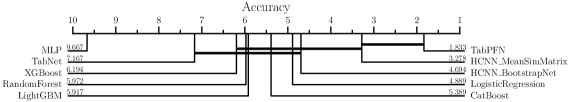
Figure 2: Critical Difference plots on out-of-sample average ranks with a Wilcoxon significance analysis. In (a) the test is run considering the F1$\_$Score; in (b) the test is run considering the accuracy; in (c) the test is run considering the MCC.

Models’ numerical performances for each evaluation metric (see app:Appendix_Dataset_Wise_Scores_Small_Tabular_Data) enforce all the findings discussed above. It is, however, clear that the differences in performance are very small. To assess their statistical significance, we use the Critical Difference (CD) diagram of the ranks based on the Wilcoxon significance test (with $p$-values below $0.1$), a standard metric for comparing classifiers across multiple datasets (Demšar, 2006). The overall empirical comparison of the methods is given in fig:Wilcoxon_Test_Small_Datasets_0_1. We notice that the performance of HCNN and TabPFN is not statistically different. This finding is coherent across the three evaluation metrics and is particularly relevant because it makes these deep learning architectures the only two which are consistently comparable with the SOTA machine learning ones. These findings legitimate the methodology proposed in the current research work as being itself a SOTA, both in terms of performance and in terms of computational complexity (see app:Appendix_Number_Of_Parameters for an extended study on the number of parameters). We cannot assert the same for the TabPFN, which is among the SOTA models in terms of performance but it is the worst model in terms of computational (and architectural) complexity.

3.2 Models’ scalability to larger tabular numerical classification problems

All the models considered in the current research work are primarily designed to handle small tabular classification problems. According to (Hollmann et al., 2022), a dataset is defined as “small” if it contains up to $2\,000$ samples and $100$ features. However, in this section, we explore the ability of the models to scale to larger problems. In doing so, we use benchmark datasets characterized, in turn, by a number of samples greater than $2\,000$ or a number of features greater than $100$.

Table 2: Study on models’ ability to scale to larger problems. Considered datasets belong to the OpenML benchmark suite “Tabular benchmark numerical classification” (Grinsztajn et al., 2022). For each of them, we report the OpenML ID, the number of samples, and the number of features. We indicate the success in solving the corresponding tabular classification task with a (✓) symbol, while a failure to solve the problem is denoted by an (✗) symbol.

OpenML ID	# Samples	# Features	Model
			LogisticRegression	RandomForest	XGBoost	LightGBM	CatBoost	MLP	TabNet	TabPFN	HCNN BootstrapNet	HCNN MeanSimMatrix
361055	16714	10	✓	✓	✓	✓	✓	✓	✓	✗	✓	✓
361062	10082	26	✓	✓	✓	✓	✓	✓	✓	✗	✓	✓
361063	13488	16	✓	✓	✓	✓	✓	✓	✓	✗	✓	✓
361065	13376	10	✓	✓	✓	✓	✓	✓	✓	✗	✓	✓
361066	10578	7	✓	✓	✓	✓	✓	✓	✓	✗	✓	✓
361275	13272	20	✓	✓	✓	✓	✓	✓	✓	✗	✓	✓
361276	3434	419	✓	✓	✓	✓	✓	✓	✓	✗	✓	✗
361277	20634	8	✓	✓	✓	✓	✓	✓	✓	✗	✓	✓
361278	10000	22	✓	✓	✓	✓	✓	✓	✓	✗	✓	✓

From tab:Scalability_Table, one can observe that the proposed datasets are sufficient in underlining the issues of two models, namely the TabPFN model and the HCNN model in its MeanSimMatrix configuration. In the first case, the model is entirely unable to scale to problems with a larger number of samples and features. This limitation was already pointed out in the original work by (Hollmann et al., 2022) and directly depends on the model’s architecture, which strongly leverage the power of attention-based mechanism. Indeed, the runtime and memory usage of the TabPFN architecture scales quadratically with the number of inputs (i.e. training samples passed) and the fitted model cannot work with datasets with a number of features $>100$. In the case of HCNN MeanSimMatrix, instead, the proposed architecture demonstrates a limit in handling problems characterised by a large number of features (but not samples). Also in this case, the reason of the failure should be searched in the model’s architectural design choices. Indeed, this architecture is characterised by a strong linear relationship between the number of features and the number of parameters (see app:Appendix_Number_Of_Parameters), meaning that when the first parameter is large, convolving across all representatives of each simplicial complex family becomes computationally demanding. A solution to this problem can be found in employing the BootstrapNet configuration, which disrupts the linear relationship discussed earlier, resulting in a significant reduction in the number of parameters when dealing with a large number of features. While this approach demonstrates considerable efficacy, it remains reliant on a threshold parameter (see sec:Information_Filtering_Networks), suggesting the need for more advanced and parameter-free alternatives. For the seek of completeness, in app:Appendix_Results_Scalability_Datasets we partially repeat the analyses presented in sec:Small_tabular_classification_results on the newly introduced datasets. Because of the fragmentation caused by the increased size, we report only the dataset-dependent analyses, excluding cross-datasets ones.

4 Conclusion

In this paper, we introduce the Homological Convolutional Neural Network (HCNN), a novel deep learning architecture that revisits the simpler Homological Neural Network (HNN) to gain abstraction, representation power, robustness, and scalability. The proposed architecture is data-centric and arises from a graph-based higher-order representation of dependency structures among multivariate input features. Compared to HNN, our model demonstrates a higher level of abstraction. Indeed, we have higher flexibility in choosing the initial network’s representation, as we can choose from the universe simplicial complexes and we are not restricted to specific sub-families. Looking at geometrical structures at different granularity levels, we propose a clear-cut way to leverage the power of convolution on sparse data representations. This allows to fully absorb the representation power of HNN in the very first layer of HCNN, leaving room for additional data transformations at deeper levels of the architecture. Specifically, in the current research work, we build the HCNN using a class of information filtering networks (i.e. the TMFG) that uses squared correlation coefficients to maximize the likelihood of the underlying system. We propose two alternative architectural solutions: (i) the MeanSimMatrix configuration; and (ii) the BootstrapNet configuration. Both of them leverage the power of bootstrapping to gain robustness toward data noise and the intrinsic complexity of interactions among the underlying system’s variables. We test these two modeling solutions on a set of tabular numerical classification problems (i.e. one of the most challenging tasks for deep learning models and the one where HNN demonstrates the poorest performances). We compare HCNN with different machine- and deep learning architectures, always teeing SOTA performances and demonstrating superior robustness to data unbalances. Specifically, we demonstrate that HCNN is able to compete with the latest transformer-based architectures (e.g. TabPFN) by using a considerably lower and easily controllable number of parameters (especially in the BootstrapNet configuration), guaranteeing a higher level of explicability in the neural network’s building process and having a comparable running time without the need for pre-training. We finally propose a study on models’ scalability to large datasets. We underline the fragility of transformer-based models and we demonstrate that HCNN in its MeanSimMatrix configuration is unable to manage datasets characterized by a large number of input features. In contrast, we show that the design choices adopted for the BootstrapNet configuration offers a parametric solution to the problem. Despite significant advances introduced by HCNNs, this class of neural networks remains in an embryonic phase. Further studies on underlying network representations should propose alternative similarity metrics that replace the squared correlation coefficients for mixed data-types (i.e. categorical and numerical or categorical only data-types), and further work is finally required to better understand low-level interactions captured by the proposed neural network model. This final point would certainly lead to a class of non-parametric, parsimonious HCNNs.

Appendix A

Tables 3 and 4 report an overview of the main characteristics of the two suites of benchmark datasets used in the current research work. In both cases the open-access of data is guaranteed by OpenML (Bischl et al., 2021). Training/validation/test split is not provided. For all the datasets, the $50\%$ of the raw dataset is used as a training set, the $25\%$ as validation set, and the remaining $25\%$ as a test set. To prove the statistical significance of results presented in the current research work, all the analyses are repeated on $10$ different combinations of training/validation/test splits. The reproducibility of results is guaranteed by a rigorous usage of seeds (i.e. $[12,\,\,190,\,\,903,\,\,7\,687,\,\,8\,279,\,\,9\,433,\,\,12\,555,\,\,22\,443,\,\,67\,822,9\,822\,127]$).

Table 3: Datasets used for models’ evaluation. These include 18 numerical tabular datasets from the OpenML-CC18 benchmark suite with at most $2\,000$ samples, $100$ features and $10$ classes. For each dataset we report the name, the number of input features, the number of samples before training/validation/test split, the number of classes, the number of samples by class and, finally, the corresponding ID number in the OpenML benchmark suite.

Dataset Name	# Features	# Samples	# Classes	Samples by Class	OpenML ID
balance-scale	4	625	3	49/288/288	11
mfeat-fourier	76	2,000	10	200/200/200/200/200/ 200/200/200/200/200	14
breast-w	9	683	2	444/239	15
mfeat-karhunen	64	2,000	10	200/200/200/200/200/ 200/200/200/200/200	16
mfeat-morphological	6	2,000	10	200/200/200/200/200/ 200/200/200/200/200	18
mfeat-zernike	47	2,000	10	200/200/200/200/200/ 200/200/200/200/200	22
diabetes	8	768	2	500/268	37
vehicle	18	846	4	218/212/217/199	54
analcatdata_authorship	70	841	4	317/296/55/173	458
pc4	37	1458	2	1280/178	1049
kc2	21	522	2	415/107	1063
pc1	21	1109	2	1032/77	1068
banknote-authentication	4	1372	2	762/610	1462
blood-transfusion-service-center	4	748	2	570/178	1464
qsar-biodeg	41	1055	2	699/356	1494
wdbc	30	569	2	357/212	1510
steel-plates-fault	27	1941	7	402/55/391/ 673/158/72/190	40982
climate-model-simulation-crashes	18	540	2	46/494	40994

The first set of data belongs to the “OpenML-CC18” benchmark suite (Hollmann et al., 2022) and is used to compare models’ performance in solving numerical classification problems, while the second set of data belongs to the “OpenML tabular benchmark numerical classification” suite (Grinsztajn et al., 2022) and is used to test the models’ ability to scale to larger problems of the same type. Looking at tab:datasets_description_table, we notice that the average number of features is $28.5$ with a standard deviation equal to $22.2$. The dataset with the lowest number of features is “balance-scale” (i.e. $4$ features) with OpenML ID $11$. The dataset with the largest number of features is “mfeat-fourier” (i.e. $76$ features) with OpenML ID $14$. All the features in all the datasets are numerical only and no missing values are detected. The average number of samples is $1191.6$ with a standard deviation equal to $557.3$. The dataset with the lowest number of samples is “kc2” (i.e. $522$ samples) with OpenML ID $1063$. The dataset with the largest number of samples is “mfeat-morphological” (i.e. $2\,000$ samples) with OpenML ID $18$. $11$ of the considered datasets are binary, while $8$ are multi-class.

Table 4: Datasets used to test models’ scalability. These include $9$ numerical tabular datasets from the OpenML “Tabular benchmark numerical classification” suite (Grinsztajn et al., 2022). All these datasets violate at least one of the selection criteria in (Hollmann et al., 2022) (i.e. they are characterised by a number of samples $>2\,000$ or they are characterised by a number of features $>100$). For each dataset we report the name, the number of input features, the number of samples before training/validation/test split, the number of classes, the number of samples by class and, finally, the corresponding ID number in the OpenML benchmark suite.

Dataset Name	# Features	# Samples	# Classes	Samples by Class	OpenML ID
credit	10	16714	2	8357/8357	361055
pol	26	10082	2	5041/5041	361062
house_16H	16	13488	2	6744/6744	361063
MagicTelescope	10	13376	2	6688/6688	361065
bank-marketing	7	10578	2	5289/5289	361066
default-of-credit-card-clients	20	13272	2	6636/6636	361275
Bioresponse	419	3434	2	1717/1717	361276
california	8	20634	2	10317/10317	361277
heloc	22	10000	2	5000/5000	361278

Looking at tab:scalability_datasets_description, we notice that the average number of features is $59.8$ with a standard deviation equal to $127.2$. The dataset with the lowest number of features is “bank-marketing” (i.e. $7$ features) with OpenML ID $361066$. The dataset with the largest number of features is “Bioresponse” (i.e. $419$ features) with OpenML ID $361276$. All the features in all the datasets are numerical only and no missing values are detected. The average number of samples is $12397.6$ with a standard deviation equal to $4523.4$. The dataset with the lowest number of samples is “Bioresponse” (i.e. $3434$ samples) with OpenML ID $361276$. The dataset with the largest number of samples is “california” (i.e. $20634$ samples) with OpenML ID $361277$. All the considered datasets are binary.

Appendix B

Data: Similarity matrix $\hat{\textbf{C}}\in\mathbb{R}^{n,n}$ from a set of observations $\{x_{1,1},\dots,x_{s,1}\},\{x_{1,2},\dots,x_{s,2}\}\dots\{x_{1,n},\dots,x_{s,n}\}$.

Result: Sparse adjacency matrix A describing the TMFG.

Function MaximumGain($\hat{\textbf{C}}$, $\mathcal{V}$, $t$):

       Initialize a vector of zeros $g\in\mathbb{R}^{1\times n}$

       for $j\in t$ do

             for $v\notin\mathcal{V}$ do

                   $\hat{\textbf{C}}_{v,j}=0$

                  

             end for

            $g=g\oplus\hat{\textbf{C}}_{v,j}$

            

       end for

      return $\max{\{g\}}$

      

Initialize four empty sets: $\mathcal{C}$ (cliques), $\mathcal{T}$ (triangles), $\mathcal{S}$ (separators), and $\mathcal{V}$ (vertices)

Initialize an adjacency matrix $\textbf{{A}}\in\mathbb{R}^{n,n}$ with all zeros

$\mathcal{C}_{1}\leftarrow$ tetrahedron, $\{v_{1},v_{2},v_{3},v_{4}\}$, obtained by choosing the $4$ entries of $\hat{\textbf{C}}$ maximizing the similarity among features

$\mathcal{T}\leftarrow$ the four triangular faces in $\mathcal{C}_{1}$: $\{v_{1},v_{2},v_{3}\}$, $\{v_{1},v_{2},v_{4}\}$, $\{v_{1},v_{3},v_{4}\}$, $\{v_{2},v_{3},v_{4}\}$

$\mathcal{V}\leftarrow$ Assign to $\mathcal{V}$ the remaining $n-4$ vertices not in $\mathcal{C}_{1}$

while $\mathcal{V}$ is not empty do

       Find the combination of $\{v_{a},v_{b},v_{c}\}\in\mathcal{T}$ (i.e. $t$) and $v_{d}\in\mathcal{V}$ which maximizes MaximumGain($\hat{\textbf{C}}$, $\mathcal{V}$, $t$)

       /* $\{v_{a},v_{b},v_{c},v_{d}\}$ is a new 4-clique $\mathcal{C}$, $\{v_{a},v_{b},v_{c}\}$ becomes a separator $\mathcal{S}$, three new triangular faces, $\{v_{a},v_{b},v_{d}\}$, $\{v_{a},v_{c},v_{d}\}$, and $\{v_{b},v_{c},v_{d}\}$ are created */

       Remove $v_{d}$ from $\mathcal{V}$

       Remove $\{v_{a},v_{b},v_{c}\}$ from $\mathcal{T}$

       Add $\{v_{a},v_{b},v_{d}\}$, $\{v_{a},v_{c},v_{d}\}$, and $\{v_{b},v_{c},v_{d}\}$ to $\mathcal{T}$

      

end while

for each pair of nodes $i,j$ in $\mathcal{C}$ do

       Set $\textbf{{A}}_{i,j}=1$

      

end for

return A

Algorithm 1 TMFG built on the similarity matrix $\hat{\textbf{C}}$ to maximize global properties of the system under analysis (e.g., likelihood).

Appendix C

[] []

Figure 3: Pictorial representations of an HNN and HCNN architectures. In Figure (a), from left to right, (i) we start from a chordal graph representing the dependency structures of features in the underlying system; (ii) we re-arrange the network’s representation to highlight the underlying simplicial complex structures (i.e. edges, triangles, tetrahedra); and (iii) we finally report a layered representation, which explicitly takes into account higher order sub-structures and their interconnections, and can be easily converted into a computational unit (i.e. a sparse MLP). In Figure (b), from left to right, (i) we start from a chordal graph representing the dependency structures of features in the underlying system; (ii) we isolate the maximal cliques corresponding to $1$-, $2$- and $3$-dimensional simplices (i.e. edges, triangles, tetrahedra) and we group them into $1$D vectors containing features’ realizations; (iii) we compute a $1^{st}$-level convolution to extract simplicial-wise non-linear relationships; (iv) we compute a $2^{nd}$-level convolution, which operates on the output of the previous level of convolution across all the representatives of each simplicial family extracting a class of non-trivial homological insights; (v) we finally apply a linear map from the $2^{nd}$-level convolution to the output, extracting model’s predictions.

Appendix D

Table 5: Hyper-parameters’ search space for all the classifiers considered in the current paper. When possible, search space is inherited from (Shwartz-Ziv et al., 2018) and (Hollmann et al., 2022).

Model	Name	Type	Value	Skip
LogisticRegression	penalty max_iter	cat int	(l1, l2, elasticnet) ($100$, $500$, $1000$)	- -
RandomForest	n_estimators max_depth min_samples_leaf min_samples_split	int int int int	[$100$, $4000$] [$10$, $50$] [$2$, $10$] [$2$, $10$]	$200$ $10$ $2$ $2$
XGBoost	n_estimators max_depth learning_rate subsample colsample_bytree colsample_bylevel alpha lambda gamma	int int float float float float float float float	[$100$, $4000$] [$1$, $10$] [$e^{-4}$, $1$] [$0.2$, $1$] [$0.2$, $1$] [$0.2$, $1$] [$e^{-4}$, $e^{2}$] [$e^{-4}$, $e^{2}$] [$e^{-4}$, $e^{2}$]	$200$ $3$ - - - - - - -
CatBoost	n_estimators max_depth learning_rate random_strength l2_leaf_reg bagging_temperature leaf_estimation_iterations	int int float int int float int	[$100$, $4000$] [$1$, $10$] [$e^{-4}$, $1$] [$1$, $10$] [$1$, $10$] [$0$, $1$] [$1$, $10$]	$300$ $3$ - $3$ $3$ - $3$
LightGBM	n_estimators max_depth learning_rate num_leaves reg_alpha reg_lambda subsample	int int float int float float float	[$100$, $4000$] [$1$, $10$] [$e^{-4}$, $1$] [$5$, $50$] ($0$, $0.01$, $1$, $2$, $5$, $7$, $10$, $50$, $100$) ($0$, $0.01$, $1$, $5$, $10$, $20$, $50$, $100$) [$0.2$, $0.8$]	$300$ $3$ - $5$ - - -
MLP	hidded_layer_sizes alpha max_iter learning_rate	int float int cat	($10$, $50$, $100$, $150$, $200$) ($0.1$, $0.01$, $0.001$, $0.0001$) ($100$, $500$, $1000$) (constant, invscaling, adaptive)	- - - -
TabNet	learning_rate n_steps relaxation_factor	float int float	[$e^{-4}$, $1$] [$1$, $8$] [$0.3$, $2$]	- - -
TabPFN	n_ensemble_configurations	int	[$8$, $128$]	$8$
HCNN BootstrapNet	n_filters_l1 n_filters_l2 tmfg_iterations tmfg_confidence tmfg_similarity	int int int float cat	[$4$, $16$] [$32$, $64$] [$100$, $1000$] ($0.90$, $0.95$, $0.99$) (pearson, spearman)	$4$ $4$ $300$ - -
HCNN MeanSimMatrix	n_filters_l1 n_filters_l2 tmfg_iterations tmfg_similarity	int int int cat	[$4$, $16$] [$32$, $64$] [$100$, $1000$] (pearson, spearman)	$4$ $4$ $300$ -

Appendix E

[] [] []

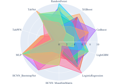
Figure 4: Out-of-sample model- and dataset-dependent average ranking considering (a) F1$\_$Score, (b) Accuracy, and (c) MCC evaluation metric. This representation allows to clearly assess the higher robustness of HCNN model to datasets’ unbalance over all its deep learning and machine learning alternatives.

All the findings related to tab:Small_Tabular_Classification_Compact_Results and discussed in sec:Small_tabular_classification_results can be graphically visualized in Figure 4. Specifically, the highest robustness of HCNN model in its MeanSimMatrix configuration compared to TabPFN model can be observed in Figure 4 and Figure 4. They report the ranking position of each model on each dataset belonging to the ”OpenML-CC18” benchmark suite using the F1_Score and the MCC as performance metrics respectively. In the first case, we notice that the worst ranking position by HCNN is $7$ and is reached when dealing with dataset “climate-model-simulation-crashes” (OpenML ID $40994$), while the one occupied by TabPFN is $10$ with dataset “pc_1” (OpenML ID $1068$). In the second case, we notice that the worst performance by HCNN has ranking $6$ and is reached when dealing with datasets “mfeat-karhunen” (OpenML ID $16$), “steel-plates-fault” (OpenML ID $40982$) and “climate-model-simulation-crashes” (OpenML ID $40994$), while the one occupied by TabPFN is $8$ with dataset “pc_1” (OpenML ID $1068$). Except for “mfeat-karhunen” dataset (OpenML ID $16$), all the datasets listed before are strongly unbalanced.

Appendix F

Table 6: For each considered model, we report the average F1_score and the corresponding standard deviation (across $10$ different seeds) on the $18$ benchmark datasets from the “OpenML-CC-18” benchmark suite.

Dataset ID	Model
	LogisticRegression	RandomForest	XGBoost	LightGBM	CatBoost	MLP	TabNet	TabPFN	HCNN BootstrapNet	HCNN MeanSimMatrix
11	0.62$\pm$0.03	0.60$\pm$0.01	0.93$\pm$0.03	0.71$\pm$0.07	0.73$\pm$0.04	0.59$\pm$0.03	0.65$\pm$0.05	0.97$\pm$0.02	0.95$\pm$0.04	0.94$\pm$0.04
14	0.79$\pm$0.01	0.82$\pm$0.02	0.81$\pm$0.02	0.81$\pm$0.02	0.82$\pm$0.01	0.77$\pm$0.03	0.82$\pm$0.01	0.82$\pm$0.01	0.81$\pm$0.01	0.82$\pm$0.02
15	0.97$\pm$0.01	0.96$\pm$0.01	0.96$\pm$0.01	0.96$\pm$0.01	0.96$\pm$0.01	0.95$\pm$0.02	0.95$\pm$0.02	0.97$\pm$0.01	0.97$\pm$0.01	0.96$\pm$0.01
16	0.95$\pm$0.01	0.96$\pm$0.01	0.95$\pm$0.00	0.95$\pm$0.01	0.96$\pm$0.01	0.94$\pm$0.01	0.96$\pm$0.01	0.97$\pm$0.01	0.94$\pm$0.01	0.96$\pm$0.01
18	0.73$\pm$0.02	0.72$\pm$0.02	0.71$\pm$0.03	0.72$\pm$0.01	0.72$\pm$0.02	0.68$\pm$0.02	0.72$\pm$0.02	0.73$\pm$0.02	0.73$\pm$0.02	0.73$\pm$0.02
22	0.82$\pm$0.01	0.77$\pm$0.02	0.79$\pm$0.01	0.78$\pm$0.01	0.79$\pm$0.02	0.77$\pm$0.03	0.80$\pm$0.03	0.82$\pm$0.02	0.82$\pm$0.02	0.82$\pm$0.01
37	0.73$\pm$0.04	0.72$\pm$0.03	0.72$\pm$0.04	0.72$\pm$0.03	0.71$\pm$0.03	0.70$\pm$0.04	0.68$\pm$0.08	0.73$\pm$0.03	0.72$\pm$0.04	0.72$\pm$0.02
54	0.76$\pm$0.03	0.73$\pm$0.03	0.77$\pm$0.04	0.76$\pm$0.04	0.77$\pm$0.04	0.67$\pm$0.06	0.80$\pm$0.04	0.84$\pm$0.03	0.82$\pm$0.03	0.83$\pm$0.03
458	1.00$\pm$0.00	0.98$\pm$0.01	0.99$\pm$0.01	0.98$\pm$0.01	0.99$\pm$0.01	0.95$\pm$0.04	0.96$\pm$0.03	1.00$\pm$0.00	0.97$\pm$0.04	0.99$\pm$0.01
1049	0.73$\pm$0.03	0.69$\pm$0.04	0.75$\pm$0.03	0.74$\pm$0.05	0.74$\pm$0.04	0.63$\pm$0.08	0.70$\pm$0.10	0.77$\pm$0.04	0.75$\pm$0.03	0.75$\pm$0.04
1063	0.68$\pm$0.05	0.70$\pm$0.04	0.64$\pm$0.11	0.71$\pm$0.05	0.70$\pm$0.03	0.62$\pm$0.09	0.58$\pm$0.09	0.69$\pm$0.06	0.68$\pm$0.06	0.68$\pm$0.05
1068	0.57$\pm$0.03	0.60$\pm$0.06	0.64$\pm$0.04	0.63$\pm$0.05	0.64$\pm$0.06	0.52$\pm$0.05	0.52$\pm$0.05	0.52$\pm$0.05	0.54$\pm$0.05	0.58$\pm$0.03
1462	0.98$\pm$0.01	0.99$\pm$0.00	0.99$\pm$0.00	1.00$\pm$0.00	1.00$\pm$0.00	0.94$\pm$0.05	0.97$\pm$0.04	1.00$\pm$0.00	1.00$\pm$0.00	1.00$\pm$0.00
1464	0.56$\pm$0.06	0.64$\pm$0.05	0.62$\pm$0.04	0.64$\pm$0.03	0.60$\pm$0.05	0.56$\pm$0.08	0.54$\pm$0.10	0.63$\pm$0.06	0.62$\pm$0.05	0.61$\pm$0.06
1494	0.85$\pm$0.02	0.83$\pm$0.02	0.83$\pm$0.02	0.84$\pm$0.02	0.82$\pm$0.02	0.81$\pm$0.04	0.78$\pm$0.13	0.86$\pm$0.01	0.83$\pm$0.02	0.84$\pm$0.02
1510	0.97$\pm$0.02	0.94$\pm$0.02	0.95$\pm$0.02	0.94$\pm$0.02	0.95$\pm$0.01	0.93$\pm$0.02	0.93$\pm$0.02	0.97$\pm$0.01	0.96$\pm$0.02	0.96$\pm$0.02
40982	0.71$\pm$0.02	0.76$\pm$0.03	0.79$\pm$0.02	0.79$\pm$0.02	0.79$\pm$0.02	0.70$\pm$0.05	0.75$\pm$0.02	0.79$\pm$0.01	0.72$\pm$0.02	0.76$\pm$0.03
40994	0.83$\pm$0.05	0.49$\pm$0.03	0.74$\pm$0.05	0.73$\pm$0.05	0.72$\pm$0.07	0.51$\pm$0.07	0.69$\pm$0.12	0.82$\pm$0.05	0.65$\pm$0.11	0.68$\pm$0.10

Table 7: For each considered model, we report the average Accuracy score and the corresponding standard deviation (across $10$ different seeds) on the $18$ benchmark datasets from the “OpenML-CC-18” benchmark suite.

Dataset ID	Model
	LogisticRegression	RandomForest	XGBoost	LightGBM	CatBoost	MLP	TabNet	TabPFN	HCNN BootstrapNet	HCNN MeanSimMatrix
11	0.88$\pm$0.02	0.86$\pm$0.02	0.97$\pm$0.01	0.87$\pm$0.08	0.90$\pm$0.02	0.85$\pm$0.04	0.89$\pm$0.02	0.99$\pm$0.01	0.98$\pm$0.01	0.98$\pm$0.01
14	0.79$\pm$0.01	0.82$\pm$0.02	0.81$\pm$0.02	0.81$\pm$0.01	0.82$\pm$0.02	0.77$\pm$0.03	0.82$\pm$0.01	0.81$\pm$0.02	0.81$\pm$0.01	0.82$\pm$0.01
15	0.97$\pm$0.01	0.96$\pm$0.01	0.96$\pm$0.01	0.96$\pm$0.01	0.97$\pm$0.01	0.95$\pm$0.02	0.96$\pm$0.02	0.97$\pm$0.01	0.97$\pm$0.01	0.97$\pm$0.01
16	0.95$\pm$0.01	0.96$\pm$0.01	0.95$\pm$0.01	0.95$\pm$0.01	0.96$\pm$0.01	0.94$\pm$0.01	0.96$\pm$0.01	0.97$\pm$0.01	0.94$\pm$0.01	0.96$\pm$0.01
18	0.74$\pm$0.02	0.72$\pm$0.02	0.71$\pm$0.02	0.72$\pm$0.02	0.72$\pm$0.02	0.70$\pm$0.02	0.74$\pm$0.01	0.73$\pm$0.02	0.74$\pm$0.02	0.74$\pm$0.02
22	0.82$\pm$0.02	0.77$\pm$0.02	0.79$\pm$0.01	0.78$\pm$0.02	0.79$\pm$0.02	0.77$\pm$0.03	0.82$\pm$0.02	0.82$\pm$0.02	0.82$\pm$0.02	0.82$\pm$0.01
37	0.76$\pm$0.03	0.75$\pm$0.03	0.74$\pm$0.04	0.74$\pm$0.03	0.73$\pm$0.03	0.73$\pm$0.03	0.73$\pm$0.05	0.76$\pm$0.03	0.75$\pm$0.04	0.76$\pm$0.02
54	0.76$\pm$0.03	0.73$\pm$0.03	0.76$\pm$0.04	0.75$\pm$0.04	0.76$\pm$0.04	0.68$\pm$0.06	0.80$\pm$0.04	0.84$\pm$0.03	0.82$\pm$0.04	0.82$\pm$0.03
458	1.00$\pm$0.00	0.99$\pm$0.01	0.99$\pm$0.00	0.99$\pm$0.01	0.99$\pm$0.01	0.96$\pm$0.03	0.97$\pm$0.02	1.00$\pm$0.00	0.98$\pm$0.02	0.99$\pm$0.01
1049	0.90$\pm$0.01	0.90$\pm$0.02	0.90$\pm$0.01	0.90$\pm$0.02	0.89$\pm$0.02	0.88$\pm$0.01	0.89$\pm$0.02	0.91$\pm$0.01	0.90$\pm$0.01	0.90$\pm$0.01
1063	0.82$\pm$0.03	0.82$\pm$0.03	0.80$\pm$0.03	0.82$\pm$0.03	0.81$\pm$0.02	0.76$\pm$0.06	0.80$\pm$0.02	0.82$\pm$0.04	0.82$\pm$0.04	0.82$\pm$0.02
1068	0.93$\pm$0.01	0.94$\pm$0.01	0.93$\pm$0.02	0.93$\pm$0.01	0.93$\pm$0.01	0.88$\pm$0.08	0.91$\pm$0.04	0.93$\pm$0.01	0.93$\pm$0.01	0.93$\pm$0.01
1462	0.98$\pm$0.01	0.99$\pm$0.00	0.99$\pm$0.00	1.00$\pm$0.00	1.00$\pm$0.00	0.94$\pm$0.05	0.97$\pm$0.04	1.00$\pm$0.00	1.00$\pm$0.00	1.00$\pm$0.00
1464	0.78$\pm$0.03	0.79$\pm$0.02	0.77$\pm$0.04	0.78$\pm$0.02	0.74$\pm$0.03	0.76$\pm$0.05	0.76$\pm$0.05	0.79$\pm$0.03	0.79$\pm$0.02	0.79$\pm$0.02
1494	0.87$\pm$0.01	0.86$\pm$0.02	0.85$\pm$0.02	0.86$\pm$0.02	0.85$\pm$0.02	0.83$\pm$0.04	0.83$\pm$0.07	0.88$\pm$0.01	0.85$\pm$0.02	0.85$\pm$0.01
1510	0.97$\pm$0.01	0.95$\pm$0.02	0.95$\pm$0.01	0.95$\pm$0.02	0.96$\pm$0.01	0.93$\pm$0.02	0.94$\pm$0.02	0.97$\pm$0.01	0.96$\pm$0.01	0.96$\pm$0.02
40982	0.71$\pm$0.02	0.75$\pm$0.03	0.77$\pm$0.02	0.78$\pm$0.02	0.78$\pm$0.01	0.72$\pm$0.02	0.73$\pm$0.01	0.77$\pm$0.02	0.71$\pm$0.02	0.75$\pm$0.01
40994	0.95$\pm$0.01	0.91$\pm$0.02	0.94$\pm$0.01	0.93$\pm$0.01	0.93$\pm$0.02	0.84$\pm$0.11	0.91$\pm$0.02	0.95$\pm$0.01	0.93$\pm$0.03	0.93$\pm$0.02

Table 8: For each considered model, we report the average MCC and the corresponding standard deviation (across $10$ different seeds) on the $18$ benchmark datasets from the “OpenML-CC-18” benchmark suite.

Dataset ID	Model
	LogisticRegression	RandomForest	XGBoost	LightGBM	CatBoost	MLP	TabNet	TabPFN	HCNN BootstrapNet	HCNN MeanSimMatrix
11	0.79$\pm$0.03	0.75$\pm$0.03	0.95$\pm$0.02	0.78$\pm$0.11	0.83$\pm$0.04	0.73$\pm$0.06	0.80$\pm$0.04	0.98$\pm$0.01	0.96$\pm$0.02	0.96$\pm$0.02
14	0.77$\pm$0.02	0.80$\pm$0.02	0.79$\pm$0.02	0.79$\pm$0.02	0.80$\pm$0.02	0.75$\pm$0.03	0.80$\pm$0.01	0.80$\pm$0.02	0.79$\pm$0.02	0.80$\pm$0.02
15	0.93$\pm$0.02	0.92$\pm$0.02	0.92$\pm$0.02	0.92$\pm$0.03	0.92$\pm$0.03	0.90$\pm$0.04	0.91$\pm$0.04	0.94$\pm$0.02	0.93$\pm$0.02	0.93$\pm$0.02
16	0.94$\pm$0.01	0.95$\pm$0.01	0.95$\pm$0.01	0.94$\pm$0.01	0.96$\pm$0.01	0.93$\pm$0.01	0.95$\pm$0.01	0.96$\pm$0.01	0.94$\pm$0.01	0.96$\pm$0.01
18	0.71$\pm$0.02	0.69$\pm$0.03	0.68$\pm$0.03	0.69$\pm$0.02	0.68$\pm$0.03	0.67$\pm$0.02	0.71$\pm$0.01	0.70$\pm$0.02	0.72$\pm$0.03	0.71$\pm$0.02
22	0.80$\pm$0.02	0.74$\pm$0.02	0.76$\pm$0.01	0.76$\pm$0.02	0.77$\pm$0.02	0.75$\pm$0.03	0.80$\pm$0.03	0.80$\pm$0.02	0.80$\pm$0.02	0.80$\pm$0.01
37	0.47$\pm$0.08	0.45$\pm$0.07	0.44$\pm$0.09	0.44$\pm$0.06	0.42$\pm$0.06	0.41$\pm$0.07	0.40$\pm$0.10	0.48$\pm$0.07	0.45$\pm$0.09	0.46$\pm$0.05
54	0.68$\pm$0.05	0.65$\pm$0.05	0.68$\pm$0.06	0.67$\pm$0.06	0.69$\pm$0.06	0.58$\pm$0.08	0.74$\pm$0.05	0.78$\pm$0.04	0.76$\pm$0.05	0.76$\pm$0.04
458	0.99$\pm$0.01	0.98$\pm$0.01	0.99$\pm$0.01	0.98$\pm$0.01	0.98$\pm$0.01	0.94$\pm$0.04	0.96$\pm$0.02	1.00$\pm$0.00	0.96$\pm$0.03	0.99$\pm$0.01
1049	0.50$\pm$0.05	0.45$\pm$0.07	0.50$\pm$0.05	0.49$\pm$0.10	0.49$\pm$0.08	0.32$\pm$0.16	0.43$\pm$0.18	0.57$\pm$0.07	0.52$\pm$0.05	0.51$\pm$0.08
1063	0.39$\pm$0.11	0.41$\pm$0.08	0.32$\pm$0.17	0.42$\pm$0.11	0.42$\pm$0.06	0.30$\pm$0.15	0.25$\pm$0.15	0.41$\pm$0.12	0.40$\pm$0.12	0.40$\pm$0.09
1068	0.20$\pm$0.05	0.28$\pm$0.12	0.30$\pm$0.08	0.30$\pm$0.10	0.30$\pm$0.13	0.07$\pm$0.10	0.06$\pm$0.09	0.09$\pm$0.13	0.14$\pm$0.13	0.25$\pm$0.08
1462	0.96$\pm$0.01	0.98$\pm$0.01	0.99$\pm$0.01	0.99$\pm$0.01	1.00$\pm$0.01	0.88$\pm$0.10	0.94$\pm$0.08	1.00$\pm$0.00	1.00$\pm$0.00	1.00$\pm$0.00
1464	0.24$\pm$0.08	0.33$\pm$0.09	0.27$\pm$0.08	0.30$\pm$0.06	0.22$\pm$0.09	0.19$\pm$0.13	0.18$\pm$0.16	0.33$\pm$0.07	0.31$\pm$0.07	0.31$\pm$0.08
1494	0.70$\pm$0.03	0.67$\pm$0.04	0.67$\pm$0.04	0.67$\pm$0.03	0.65$\pm$0.04	0.63$\pm$0.07	0.60$\pm$0.20	0.73$\pm$0.03	0.66$\pm$0.04	0.67$\pm$0.03
1510	0.93$\pm$0.03	0.88$\pm$0.04	0.90$\pm$0.03	0.89$\pm$0.04	0.90$\pm$0.02	0.86$\pm$0.04	0.87$\pm$0.04	0.93$\pm$0.02	0.92$\pm$0.03	0.92$\pm$0.03
40982	0.62$\pm$0.03	0.68$\pm$0.03	0.70$\pm$0.03	0.71$\pm$0.02	0.72$\pm$0.02	0.63$\pm$0.03	0.65$\pm$0.02	0.70$\pm$0.02	0.62$\pm$0.03	0.67$\pm$0.02
40994	0.68$\pm$0.10	0.03$\pm$0.10	0.53$\pm$0.08	0.51$\pm$0.09	0.49$\pm$0.13	0.07$\pm$0.11	0.39$\pm$0.25	0.65$\pm$0.11	0.38$\pm$0.24	0.43$\pm$0.18

Appendix G

[] [] []

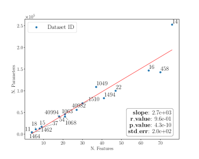
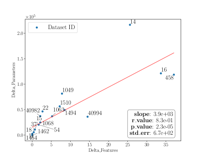
Figure 5: Study of the relationship between the number of total features ($x$-axis) and the number of parameters ($y$-axis) for the (a) HCNN MeanSimMatrix and (b) HCNN BootstrapNet configuration. Figure (c) reports the relationship structure among the difference in the number of features ($x$-axis) and the difference in the number of total parameters ($y$-axis) when using the two above-mentioned configurations.

Figure 5 reports the relationship between the number of features and the total number of parameters for the HCNN in its MeanSimMatrix configuration, the relationship between the number of features and the total number of parameters for the HCNN in its BootstrapNet configuration and the relationship between the difference in the number of features and the difference in the total number of parameters in the two configurations. Looking at Figure 5, it is possible to conclude that a strong linear relationship exists between the number of features and the total number of parameters of the HCNN model in the MeanSimMatrix configuration. This finding was expected since the proposed model’s architecture entirely depends on the complete homological structure of the underlying system. This means that, each time a new feature is introduced, we could potentially observe an increase in the number of edges, triangles, and tetrahedra, which in turn determines a proportional increase in the number of parameters of the HCNN itself. On this point, we need to underline that the magnitude of the slope of the regression line heavily depends on the optimal hyper-parameters describing the number of filters in the two convolutional layers. Looking at Figure 5, we observe again a relatively strong linear relationship between the number of features and the total number of parameters of the HCNN model in the BootstrapNet configuration. The difference in r_value between the two configurations is equal to $0.19$ and depends on the fact that, in the second case, the optimal threshold value which maximizes the model’s performance (different across datasets), does not depend on the number of inputs features and determines the ablation of a number of features that has no dependence with any other factor. More generally, in the BootstrapNet configuration, we observe a number of parameters that is, on average, one order of magnitude below the one in the HCNN MeanSimMatrix configuration. To better study this finding, in Figure 5 we report, on the $x$-axis the difference in the number of features $\Delta_{f}$ and on $y$-axis the difference in the number of parameters $\Delta_{p}$. As one can see, the linear relationship is strong only when the two deltas are low. For higher deltas, specifically for the three datasets “mfeat-fourier” (OpenML ID $14$), “mfeat-karhunen” (OpenML ID $16$), and “analcatdata_authorship” (OpenML ID $458$), even if the decrement is significant for both parameters, the relationship is not linear.

Appendix H

Table 9: For each considered model, we report the average F1_score and the corresponding standard deviation (across $10$ different seeds) on the $9$ benchmark datasets from the “OpenML tabular benchmark numerical classification” suite. The symbol ”/” denotes the inability of the model to achieve convergence within the time or computing resources allocated for the corresponding learning task.

Dataset ID	Model
	LogisticRegression	RandomForest	XGBoost	LightGBM	CatBoost	MLP	TabNet	TabPFN	HCNN BootstrapNet	HCNN MeanSimMatrix
361055	0.72$\pm$0.01	0.78$\pm$0.00	0.77$\pm$0.00	0.78$\pm$0.00	0.78$\pm$0.00	0.75$\pm$0.01	0.66$\pm$0.14	/	0.77$\pm$0.01	0.76$\pm$0.01
361062	0.86$\pm$0.01	0.98$\pm$0.00	0.98$\pm$0.00	0.98$\pm$0.00	0.98$\pm$0.00	0.97$\pm$0.00	0.98$\pm$0.00	/	0.99$\pm$0.00	0.99$\pm$0.00
361063	0.82$\pm$0.01	0.88$\pm$0.01	0.88$\pm$0.01	0.88$\pm$0.01	0.88$\pm$0.00	0.86$\pm$0.00	0.86$\pm$0.01	/	0.88$\pm$0.01	0.88$\pm$0.01
361065	0.77$\pm$0.01	0.86$\pm$0.00	0.86$\pm$0.01	0.86$\pm$0.01	0.86$\pm$0.00	0.84$\pm$0.01	0.86$\pm$0.01	/	0.82$\pm$0.03	0.85$\pm$0.00
361066	0.74$\pm$0.01	0.80$\pm$0.01	0.80$\pm$0.01	0.80$\pm$0.01	0.80$\pm$0.01	0.78$\pm$0.01	0.79$\pm$0.01	/	0.80$\pm$0.01	0.79$\pm$0.00
361275	0.67$\pm$0.01	0.71$\pm$0.01	0.71$\pm$0.01	0.71$\pm$0.01	0.71$\pm$0.01	0.70$\pm$0.01	0.70$\pm$0.01	/	0.70$\pm$0.01	0.70$\pm$0.01
361276	0.73$\pm$0.02	0.78$\pm$0.01	0.78$\pm$0.02	0.78$\pm$0.02	0.78$\pm$0.02	0.75$\pm$0.02	0.71$\pm$0.03	/	0.72$\pm$0.02	/
361277	0.83$\pm$0.01	0.89$\pm$0.00	0.90$\pm$0.00	0.90$\pm$0.00	0.90$\pm$0.00	0.86$\pm$0.01	0.84$\pm$0.02	/	0.88$\pm$0.01	0.88$\pm$0.00
361278	0.71$\pm$0.01	0.72$\pm$0.01	0.72$\pm$0.01	0.72$\pm$0.01	0.72$\pm$0.01	0.71$\pm$0.01	0.71$\pm$0.01	/	0.72$\pm$0.01	0.72$\pm$0.01

Table 10: For each considered model, we report the average Accuracy score and the corresponding standard deviation (across $10$ different seeds) on the $9$ benchmark datasets from the “OpenML tabular benchmark numerical classification” suite. The symbol ”/” denotes the inability of the model to achieve convergence within the time or computing resources allocated for the corresponding learning task.

Dataset ID	Model
	LogisticRegression	RandomForest	XGBoost	LightGBM	CatBoost	MLP	TabNet	TabPFN	HCNN BootstrapNet	HCNN MeanSimMatrix
361055	0.72$\pm$0.01	0.78$\pm$0.00	0.77$\pm$0.00	0.78$\pm$0.00	0.78$\pm$0.00	0.75$\pm$0.01	0.69$\pm$0.09	/	0.77$\pm$0.01	0.76$\pm$0.01
361062	0.86$\pm$0.01	0.98$\pm$0.00	0.98$\pm$0.00	0.98$\pm$0.00	0.98$\pm$0.00	0.97$\pm$0.00	0.98$\pm$0.00	/	0.99$\pm$0.00	0.99$\pm$0.00
361063	0.82$\pm$0.01	0.88$\pm$0.01	0.88$\pm$0.01	0.88$\pm$0.01	0.88$\pm$0.00	0.86$\pm$0.00	0.86$\pm$0.01	/	0.88$\pm$0.01	0.88$\pm$0.01
361065	0.77$\pm$0.01	0.86$\pm$0.00	0.86$\pm$0.01	0.86$\pm$0.01	0.86$\pm$0.00	0.84$\pm$0.01	0.86$\pm$0.01	/	0.82$\pm$0.03	0.85$\pm$0.00
361066	0.75$\pm$0.01	0.80$\pm$0.01	0.80$\pm$0.01	0.80$\pm$0.01	0.80$\pm$0.01	0.78$\pm$0.01	0.79$\pm$0.01	/	0.80$\pm$0.01	0.79$\pm$0.00
361275	0.67$\pm$0.01	0.71$\pm$0.01	0.71$\pm$0.01	0.71$\pm$0.01	0.71$\pm$0.01	0.70$\pm$0.01	0.70$\pm$0.01	/	0.71$\pm$0.01	0.71$\pm$0.01
361276	0.73$\pm$0.02	0.78$\pm$0.01	0.78$\pm$0.02	0.78$\pm$0.02	0.78$\pm$0.02	0.75$\pm$0.02	0.71$\pm$0.03	/	0.73$\pm$0.02	/
361277	0.83$\pm$0.01	0.89$\pm$0.00	0.90$\pm$0.00	0.90$\pm$0.00	0.90$\pm$0.00	0.86$\pm$0.01	0.84$\pm$0.02	/	0.88$\pm$0.01	0.88$\pm$0.00
361278	0.71$\pm$0.01	0.72$\pm$0.01	0.72$\pm$0.01	0.72$\pm$0.01	0.72$\pm$0.01	0.71$\pm$0.01	0.71$\pm$0.01	/	0.72$\pm$0.01	0.72$\pm$0.01

Table 11: For each considered model, we report the average MCC and the corresponding standard deviation (across $10$ different seeds) on the $9$ benchmark datasets from the “OpenML tabular benchmark numerical classification” suite. The symbol ”/” denotes the inability of the model to achieve convergence within the time or computing resources allocated for the corresponding learning task.

Dataset ID	Model
	LogisticRegression	RandomForest	XGBoost	LightGBM	CatBoost	MLP	TabNet	TabPFN	HCNN BootstrapNet	HCNN MeanSimMatrix
361055	0.45$\pm$0.03	0.56$\pm$0.01	0.55$\pm$0.01	0.55$\pm$0.01	0.55$\pm$0.00	0.50$\pm$0.02	0.41$\pm$0.15	/	0.53$\pm$0.02	0.52$\pm$0.02
361062	0.72$\pm$0.01	0.96$\pm$0.01	0.96$\pm$0.00	0.97$\pm$0.00	0.97$\pm$0.00	0.95$\pm$0.00	0.96$\pm$0.01	/	0.97$\pm$0.00	0.97$\pm$0.00
361063	0.65$\pm$0.02	0.76$\pm$0.01	0.76$\pm$0.01	0.77$\pm$0.01	0.76$\pm$0.01	0.73$\pm$0.01	0.72$\pm$0.02	/	0.75$\pm$0.01	0.75$\pm$0.01
361065	0.55$\pm$0.01	0.72$\pm$0.01	0.72$\pm$0.01	0.72$\pm$0.01	0.72$\pm$0.01	0.69$\pm$0.01	0.72$\pm$0.01	/	0.64$\pm$0.05	0.71$\pm$0.01
361066	0.49$\pm$0.01	0.60$\pm$0.01	0.60$\pm$0.02	0.60$\pm$0.01	0.60$\pm$0.02	0.56$\pm$0.02	0.57$\pm$0.01	/	0.59$\pm$0.01	0.59$\pm$0.01
361275	0.34$\pm$0.02	0.43$\pm$0.02	0.42$\pm$0.01	0.42$\pm$0.01	0.42$\pm$0.02	0.41$\pm$0.01	0.42$\pm$0.02	/	0.42$\pm$0.01	0.42$\pm$0.01
361276	0.47$\pm$0.03	0.56$\pm$0.02	0.57$\pm$0.03	0.55$\pm$0.04	0.55$\pm$0.03	0.50$\pm$0.05	0.43$\pm$0.06	/	0.45$\pm$0.04	/
361277	0.66$\pm$0.02	0.78$\pm$0.01	0.81$\pm$0.01	0.81$\pm$0.01	0.81$\pm$0.01	0.72$\pm$0.02	0.69$\pm$0.04	/	0.76$\pm$0.02	0.76$\pm$0.01
361278	0.42$\pm$0.02	0.44$\pm$0.01	0.44$\pm$0.02	0.44$\pm$0.02	0.44$\pm$0.02	0.43$\pm$0.02	0.42$\pm$0.02	/	0.43$\pm$0.02	0.44$\pm$0.02

References

- Arik and Pfister (2021) Sercan Ö Arik and Tomas Pfister. Tabnet: Attentive interpretable tabular learning. In Proceedings of the AAAI Conference on Artificial Intelligence, volume 35, pages 6679–6687, 2021.
- Aste (2022) Tomaso Aste. Topological regularization with information filtering networks. Information Sciences, 608:655–669, 2022.
- Aste et al. (2005) Tomaso Aste, Tiziana Di Matteo, and ST Hyde. Complex networks on hyperbolic surfaces. Physica A: Statistical Mechanics and its Applications, 346(1-2):20–26, 2005.
- Badirli et al. (2020) Sarkhan Badirli, Xuanqing Liu, Zhengming Xing, Avradeep Bhowmik, Khoa Doan, and Sathiya S Keerthi. Gradient boosting neural networks: Grownet. arXiv preprint arXiv:2002.07971, 2020.
- Baosenguo (2021) Baosenguo. baosenguo/kaggle-moa-2nd-place-solution. https://github.com/baosenguo/Kaggle-MoA-2nd-Place-Solution, 2021. Online; accessed 07-June-2023.
- Barfuss et al. (2016) Wolfram Barfuss, Guido Previde Massara, Tiziana Di Matteo, and Tomaso Aste. Parsimonious modeling with information filtering networks. Physical Review E, 94(6):062306, 2016.
- Beutel et al. (2018) Alex Beutel, Paul Covington, Sagar Jain, Can Xu, Jia Li, Vince Gatto, and Ed H Chi. Latent cross: Making use of context in recurrent recommender systems. In Proceedings of the Eleventh ACM International Conference on Web Search and Data Mining, pages 46–54, 2018.
- Bischl et al. (2017) Bernd Bischl, Giuseppe Casalicchio, Matthias Feurer, Pieter Gijsbers, Frank Hutter, Michel Lang, Rafael G Mantovani, Jan N van Rijn, and Joaquin Vanschoren. Openml benchmarking suites. arXiv preprint arXiv:1708.03731, 2017.
- Bischl et al. (2021) Bernd Bischl, Giuseppe Casalicchio, Matthias Feurer, Pieter Gijsbers, Frank Hutter, Michel Lang, Rafael Gomes Mantovani, Jan N. van Rijn, and Joaquin Vanschoren. Openml: A benchmarking layer on top of openml to quickly create, download, and share systematic benchmarks. NeurIPS, 2021. URL https://openreview.net/forum?id=OCrD8ycKjG.
- Bose and Tripathy (2020) Ankita Bose and BK Tripathy. Deep learning for audio signal classification. Deep learning research and applications, pages 105–136, 2020.
- Briola and Aste (2022) Antonio Briola and Tomaso Aste. Dependency structures in cryptocurrency market from high to low frequency. arXiv preprint arXiv:2206.03386, 2022.
- Briola and Aste (2023) Antonio Briola and Tomaso Aste. Topological feature selection. In Topological, Algebraic and Geometric Learning Workshops 2023, pages 534–556. PMLR, 2023.
- Briola et al. (2022) Antonio Briola, David Vidal-Tomás, Yuanrong Wang, and Tomaso Aste. Anatomy of a stablecoin’s failure: The terra-luna case. Finance Research Letters, page 103358, 2022.
- Buczak and Guven (2015) Anna L Buczak and Erhan Guven. A survey of data mining and machine learning methods for cyber security intrusion detection. IEEE Communications surveys & tutorials, 18(2):1153–1176, 2015.
- Chen and Guestrin (2016) Tianqi Chen and Carlos Guestrin. Xgboost: A scalable tree boosting system. In Proceedings of the 22nd acm sigkdd international conference on knowledge discovery and data mining, pages 785–794, 2016.
- Chowdhary and Chowdhary (2020) KR1442 Chowdhary and KR Chowdhary. Natural language processing. Fundamentals of artificial intelligence, pages 603–649, 2020.
- Demšar (2006) Janez Demšar. Statistical comparisons of classifiers over multiple data sets. The Journal of Machine learning research, 7:1–30, 2006.
- Dua et al. (2017) Dheeru Dua, Casey Graff, et al. Uci machine learning repository. 2017.
- Efron et al. (1996) Bradley Efron, Elizabeth Halloran, and Susan Holmes. Bootstrap confidence levels for phylogenetic trees. Proceedings of the National Academy of Sciences, 93(23):13429–13429, 1996.
- Friedman (2001) Jerome H Friedman. Greedy function approximation: a gradient boosting machine. Annals of statistics, pages 1189–1232, 2001.
- Grinsztajn et al. (2022) Léo Grinsztajn, Edouard Oyallon, and Gaël Varoquaux. Why do tree-based models still outperform deep learning on tabular data? arXiv preprint arXiv:2207.08815, 2022.
- Hazimeh et al. (2020) Hussein Hazimeh, Natalia Ponomareva, Petros Mol, Zhenyu Tan, and Rahul Mazumder. The tree ensemble layer: Differentiability meets conditional computation. In International Conference on Machine Learning, pages 4138–4148. PMLR, 2020.
- He et al. (2015) Kaiming He, Xiangyu Zhang, Shaoqing Ren, and Jian Sun. Delving deep into rectifiers: Surpassing human-level performance on imagenet classification. In Proceedings of the IEEE international conference on computer vision, pages 1026–1034, 2015.
- Hollmann et al. (2022) Noah Hollmann, Samuel Müller, Katharina Eggensperger, and Frank Hutter. Tabpfn: A transformer that solves small tabular classification problems in a second. arXiv preprint arXiv:2207.01848, 2022.
- Huang et al. (2020) Xin Huang, Ashish Khetan, Milan Cvitkovic, and Zohar Karnin. Tabtransformer: Tabular data modeling using contextual embeddings. arXiv preprint arXiv:2012.06678, 2020.
- Ihara (1993) Shunsuke Ihara. Information theory for continuous systems, volume 2. World Scientific, 1993.
- Kadra et al. (2021a) Arlind Kadra, Marius Lindauer, Frank Hutter, and Josif Grabocka. Regularization is all you need: Simple neural nets can excel on tabular data. arXiv preprint arXiv:2106.11189, 536, 2021a.
- Kadra et al. (2021b) Arlind Kadra, Marius Lindauer, Frank Hutter, and Josif Grabocka. Well-tuned simple nets excel on tabular datasets. Advances in neural information processing systems, 34:23928–23941, 2021b.
- Ke et al. (2017) Guolin Ke, Qi Meng, Thomas Finley, Taifeng Wang, Wei Chen, Weidong Ma, Qiwei Ye, and Tie-Yan Liu. Lightgbm: A highly efficient gradient boosting decision tree. Advances in neural information processing systems, 30, 2017.
- Klambauer et al. (2017) Günter Klambauer, Thomas Unterthiner, Andreas Mayr, and Sepp Hochreiter. Self-normalizing neural networks. Advances in neural information processing systems, 30, 2017.
- Kontschieder et al. (2015) Peter Kontschieder, Madalina Fiterau, Antonio Criminisi, and Samuel Rota Bulo. Deep neural decision forests. In Proceedings of the IEEE international conference on computer vision, pages 1467–1475, 2015.
- Kullback and Leibler (1951) Solomon Kullback and Richard A Leibler. On information and sufficiency. The annals of mathematical statistics, 22(1):79–86, 1951.
- Lai et al. (2015) Siwei Lai, Liheng Xu, Kang Liu, and Jun Zhao. Recurrent convolutional neural networks for text classification. In Proceedings of the AAAI conference on artificial intelligence, volume 29, 2015.
- Mantegna (1999) Rosario N Mantegna. Hierarchical structure in financial markets. The European Physical Journal B-Condensed Matter and Complex Systems, 11(1):193–197, 1999.
- Massara et al. (2017) Guido Previde Massara, Tiziana Di Matteo, and Tomaso Aste. Network filtering for big data: Triangulated maximally filtered graph. Journal of complex Networks, 5(2):161–178, 2017.
- Ohana et al. (2021) Jean Jacques Ohana, Steve Ohana, Eric Benhamou, David Saltiel, and Beatrice Guez. Explainable ai (xai) models applied to the multi-agent environment of financial markets. In Explainable and Transparent AI and Multi-Agent Systems: Third International Workshop, EXTRAAMAS 2021, Virtual Event, May 3–7, 2021, Revised Selected Papers 3, pages 189–207. Springer, 2021.
- Osman et al. (2003) Ibrahim H Osman, Baydaa Al-Ayoubi, and Musbah Barake. A greedy random adaptive search procedure for the weighted maximal planar graph problem. Computers & industrial engineering, 45(4):635–651, 2003.
- Pak and Kim (2017) Myeongsuk Pak and Sanghoon Kim. A review of deep learning in image recognition. In 2017 4th international conference on computer applications and information processing technology (CAIPT), pages 1–3. IEEE, 2017.
- Pang et al. (2022) Guansong Pang, Charu Aggarwal, Chunhua Shen, and Nicu Sebe. Editorial deep learning for anomaly detection. IEEE Transactions on Neural Networks and Learning Systems, 33(6):2282–2286, 2022.
- Popov et al. (2019) Sergei Popov, Stanislav Morozov, and Artem Babenko. Neural oblivious decision ensembles for deep learning on tabular data. arXiv preprint arXiv:1909.06312, 2019.
- Prokhorenkova et al. (2018) Liudmila Prokhorenkova, Gleb Gusev, Aleksandr Vorobev, Anna Veronika Dorogush, and Andrey Gulin. Catboost: unbiased boosting with categorical features. Advances in neural information processing systems, 31, 2018.
- Purwins et al. (2019) Hendrik Purwins, Bo Li, Tuomas Virtanen, Jan Schlüter, Shuo-Yiin Chang, and Tara Sainath. Deep learning for audio signal processing. IEEE Journal of Selected Topics in Signal Processing, 13(2):206–219, 2019.
- Rawat et al. (2019) Danda B Rawat, Ronald Doku, and Moses Garuba. Cybersecurity in big data era: From securing big data to data-driven security. IEEE Transactions on Services Computing, 14(6):2055–2072, 2019.
- Sachan et al. (2020) Swati Sachan, Jian-Bo Yang, Dong-Ling Xu, David Eraso Benavides, and Yang Li. An explainable ai decision-support-system to automate loan underwriting. Expert Systems with Applications, 144:113100, 2020.
- Salnikov et al. (2018) Vsevolod Salnikov, Daniele Cassese, and Renaud Lambiotte. Simplicial complexes and complex systems. European Journal of Physics, 40(1):014001, 2018.
- Shavitt and Segal (2018) Ira Shavitt and Eran Segal. Regularization learning networks: deep learning for tabular datasets. Advances in Neural Information Processing Systems, 31, 2018.
- Shwartz-Ziv and Armon (2022) Ravid Shwartz-Ziv and Amitai Armon. Tabular data: Deep learning is not all you need. Information Fusion, 81:84–90, 2022.
- Shwartz-Ziv et al. (2018) Ravid Shwartz-Ziv, Amichai Painsky, and Naftali Tishby. Representation compression and generalization in deep neural networks, 2018.
- Somani et al. (2021) Sulaiman Somani, Adam J Russak, Felix Richter, Shan Zhao, Akhil Vaid, Fayzan Chaudhry, Jessica K De Freitas, Nidhi Naik, Riccardo Miotto, Girish N Nadkarni, et al. Deep learning and the electrocardiogram: review of the current state-of-the-art. EP Europace, 23(8):1179–1191, 2021.
- Somepalli et al. (2021) Gowthami Somepalli, Micah Goldblum, Avi Schwarzschild, C Bayan Bruss, and Tom Goldstein. Saint: Improved neural networks for tabular data via row attention and contrastive pre-training. arXiv preprint arXiv:2106.01342, 2021.
- Song et al. (2019) Weiping Song, Chence Shi, Zhiping Xiao, Zhijian Duan, Yewen Xu, Ming Zhang, and Jian Tang. Autoint: Automatic feature interaction learning via self-attentive neural networks. In Proceedings of the 28th ACM International Conference on Information and Knowledge Management, pages 1161–1170, 2019.
- Torres and Bianconi (2020) Joaquín J Torres and Ginestra Bianconi. Simplicial complexes: higher-order spectral dimension and dynamics. Journal of Physics: Complexity, 1(1):015002, 2020.
- Tumminello et al. (2005) Michele Tumminello, Tomaso Aste, Tiziana Di Matteo, and Rosario N Mantegna. A tool for filtering information in complex systems. Proceedings of the National Academy of Sciences, 102(30):10421–10426, 2005.
- Tumminello et al. (2007) Michele Tumminello, Claudia Coronnello, Fabrizio Lillo, Salvatore Micciche, and Rosario N Mantegna. Spanning trees and bootstrap reliability estimation in correlation-based networks. International Journal of Bifurcation and Chaos, 17(07):2319–2329, 2007.
- Ulmer et al. (2020) Dennis Ulmer, Lotta Meijerink, and Giovanni Cinà. Trust issues: Uncertainty estimation does not enable reliable ood detection on medical tabular data. In Machine Learning for Health, pages 341–354. PMLR, 2020.
- Vidal-Tomás et al. (2023) David Vidal-Tomás, Antonio Briola, and Tomaso Aste. Ftx’s downfall and binance’s consolidation: the fragility of centralized digital finance. arXiv preprint arXiv:2302.11371, 2023.
- Wang et al. (2019) Qiang Wang, Bei Li, Tong Xiao, Jingbo Zhu, Changliang Li, Derek F Wong, and Lidia S Chao. Learning deep transformer models for machine translation. arXiv preprint arXiv:1906.01787, 2019.
- Wang et al. (2022) Siqi Wang, Jiyuan Liu, Guang Yu, Xinwang Liu, Sihang Zhou, En Zhu, Yuexiang Yang, Jianping Yin, and Wenjing Yang. Multiview deep anomaly detection: A systematic exploration. IEEE Transactions on Neural Networks and Learning Systems, 2022.
- Wang et al. (2023a) Yuanrong Wang, Antonio Briola, and Tomaso Aste. Homological neural networks: A sparse architecture for multivariate complexity, 2023a.
- Wang et al. (2023b) Yuanrong Wang, Antonio Briola, and Tomaso Aste. Topological portfolio selection and optimization. arXiv preprint arXiv:2310.14881, 2023b.
- Zhang and Li (2021) Min Zhang and Juntao Li. A commentary of gpt-3 in mit technology review 2021. Fundamental Research, 1(6):831–833, 2021.
- Zhang et al. (2021) Qi Zhang, Longbing Cao, Chongyang Shi, and Zhendong Niu. Neural time-aware sequential recommendation by jointly modeling preference dynamics and explicit feature couplings. IEEE Transactions on Neural Networks and Learning Systems, 33(10):5125–5137, 2021.
- Zhang et al. (2019a) Shuai Zhang, Lina Yao, Aixin Sun, and Yi Tay. Deep learning based recommender system: A survey and new perspectives. ACM computing surveys (CSUR), 52(1):1–38, 2019a.
- Zhang et al. (2019b) Zihao Zhang, Stefan Zohren, and Stephen Roberts. Deeplob: Deep convolutional neural networks for limit order books. IEEE Transactions on Signal Processing, 67(11):3001–3012, 2019b.