DeLELSTM: Decomposition-based Linear Explainable LSTM to Capture Instantaneous and Long-term Effects in Time Series

Abstract

Time series forecasting is prevalent in various real-world applications. Despite the promising results of deep learning models in time series forecasting, especially the Recurrent Neural Networks (RNNs), the explanations of time series models, which are critical in high-stakes applications, have received little attention. In this paper, we propose a Decomposition-based Linear Explainable LSTM (DeLELSTM) to improve the interpretability of LSTM. Conventionally, the interpretability of RNNs only concentrates on the variable importance and time importance. We additionally distinguish between the instantaneous influence of new coming data and the long-term effects of historical data. Specifically, DeLELSTM consists of two components, i.e., standard LSTM and tensorized LSTM. The tensorized LSTM assigns each variable with a unique hidden state making up a matrix $\mathbf{h}_{t}$, and the standard LSTM models all the variables with a shared hidden state $\mathbf{H}_{t}$. By decomposing the $\mathbf{H}_{t}$ into the linear combination of past information $\mathbf{h}_{t-1}$ and the fresh information $\mathbf{h}_{t}-\mathbf{h}_{t-1}$, we can get the instantaneous influence and the long-term effect of each variable. In addition, the advantage of linear regression also makes the explanation transparent and clear. We demonstrate the effectiveness and interpretability of DeLELSTM on three empirical datasets. Extensive experiments show that the proposed method achieves competitive performance against the baseline methods and provides a reliable explanation relative to domain knowledge.

1 Introduction

Time series forecasting is ubiquitous across a broad range of applications, including finance [1], meteorology [2], energy consumption [3], and medical health [4]. Deep neural networks have been successfully developed for time series forecasting tasks. Among them, Recurrent Neural Networks (RNNs) and its variant, the Long-Short Term Memory (LSTM) [5] and the Gated Recurrent Units (GRU) [6], are widely used networks for handling sequential data and have been proven to be powerful tools [7].

Despite the promising results of RNNs in time series forecasting, using RNNs to modelling time series lack interpretability, which is critical in high-stakes applications like finance and healthcare. For example, in the medical field, e.g., predicting the mortality rate after patients enter the ICU, it is crucial for clinicians to understand how models output a specific prediction and which indicators are useful. Such explanations can aid reliable decision-making for clinicians and increase trust in models’ predictions.

Although much recent work has been done on explainability in the computer vision and natural language processing [8, 9, 10], this problem has been overlooked in the case of time series forecasting [11, 12, 13]. The time series is special because of its dynamic nature, which causes multivariable patterns to change over time and makes it more difficult to build explainable models.

There are two main challenges in explaining time series forecasting models. First, each variable has a different impact on the target series, and the effects of variables on the target series are dynamic over time. Therefore, capturing the different dynamic impacts of each variable and distinguishing the contribution of each variable to the prediction is difficult for explaining the forecasting model. Second, the serial dependencies for each variable are heterogeneous. When predicting target series, the long-term effects of some variables play a decisive role, while the instantaneous effect of other variables is more important. For example, in the financial market, investors tend to utilize multivariate time series, such as the stock index and related stocks, to forecast the stock prices at the next time point. If the instantaneous influence and the long-term effects of each feature can be distinguished, investors can focus on more significant information and make appropriate investment decisions. As a result, we should solve the challenge of distinguishing the long-term effect and the instantaneous influence of each variable.

Existing explainable RNNs primarily use the attention mechanism on the hidden states to get the important variables [11, 7]. The hidden states involve information from previous steps and the new inputs of all variables, but none of these methods explicitly model the immediate impact of fresh information and the long-term effects of historical data. In addition, whether the attention mechanism can be directly applied to model interpretation is still controversial [14, 15]. Moreover, most of the explainable studies just make predictions once based on historical data and ignore the importance of real-time series forecasting, which predicts at each time point. For example, predicting electricity consumption at each hour is crucial for electric power providers to maximize resource utilization and cut costs.

To address these challenges, we propose DeLELSTM: Decomposed-based Linear Explainable LSTM, which simultaneously: (i) identifies the instantaneous influence and long-term effects of each variable; (ii) leverages the linearity of linear regression to make interpretation transparent and straightforward. Specifically, DeLELSTM involves two components. One is standard LSTM, in which the hidden state $\mathbf{H}_{t}$ encapsulates information of all variables until time $t$. The other is tensorized LSTM [16], where the hidden state $\mathbf{h}_{t}$ is a matrice and each row of the hidden state only encodes information exclusively from a certain variable of the input. To capture the instantaneous influence and long-term effects of each variable, the linear combination of the hidden state at time $t-1$ and the dynamic change of the hidden state at time $t$ of each variable is used to approximate the $\mathbf{H}_{t}$. The linearity of the linear regression can make the explanation transparent and clear. In addition, given the significance of real-time forecasting in time series, we aim to build an explainable model for real-time series forecasting.

The major contributions of this work are as follows:

• We consider the instantaneous influence and long-term effects of each variable, which commonly exists in time series data.

• We take advantage of the explanation of the linear regression model to make a clear and transparent explanation.

• Extensive experiments with three benchmark datasets show that DeLELSTM can achieve competitive performance and provide transparent explanations relative to domain knowledge.

The rest of the paper is organized as follows. Section 2 reviews the related work. Section 3 introduces the problem definition and details our proposed framework. Then we evaluate our method by comparing it with several baselines in Section 4 and conclude in Section 5.

2 Related Work

In recent years, different classes of approaches have been proposed to explain time series forecasting models, especially RNNs. One general approach is post-hoc analysis, which explains the models by evaluating the importance of each variable in the predictions. The other is ante-hoc methods, which incorporate interpretability directly into their structures.

Post-hoc methods frequently adopt variable-level attribution interpretations, also known as salience maps [17]. These methods assign a relevance score to each variable, indicating how sensitive a variable is to the output. Gradient-based and perturbation-based methods are the two main types of attribution methods. Gradient-based methods examine the characteristics to which output was most sensitive [18, 19, 20, 21]. In perturbation-based approaches, the variable importance is obtained by perturbing the variables with mean value or random uniform noise, running a forward pass on the new put, and comparing the difference to the original output [22, 23]. However, these post-hoc explainable models have been criticized for failing to capture the sequential dependencies and clarifying how the underlying model arrived at a specific prediction [11, 24].

On the other hand, ante-hoc models can provide intrinsic explanations by building self-explanatory systems. Among ante-hoc models, attention-based interpretable models are widely used for explaining RNNs. The parameters of these models, known as attention weights, are utilized to explain how the models behave over time. For example,  [25] proposed RETAIN, an explainable model based on a two-level attention mechanism. Two sets of attention scores are used to identify relevant clinical variables and influential hospital visits, respectively.  [7] proposed a mixture attention framework to get variable importance and temporal importance. However, the focus of the current attention mechanism is on hidden states, which encode information from both past and new observations. Differentiating between the immediate impact of new information and the long-term effects of historical data can be difficult. In addition, attention’s interpretability is still debatable  [14], and other studies found that attention patterns cannot reliably provide transparent and reliable explanations  [26].

In this paper, we propose a decomposition-based method to decompose hidden states at each time step into two components, representing instantaneous information and historical information, respectively. In addition, the linear regression model is utilized to build a transparent and faithful explainable model for time series forecasting.

3 The Proposed Framework - DeLELSTM

3.1 Problem Definition

Let $\textbf{X}\in\mathbb{R}^{D\times T}$ be a sample of a multivariate time-series data where $D$ is the number of variables with $T$ observations over time. Further, $\mathbf{x}_{t}\in\mathbb{R}^{D}$ is the set of all observations at time $t\in[1,\cdots,T]$, denoted by the vector $[x_{t}^{1},x_{t}^{2},\cdots,x_{t}^{D}]$ and $\mathbf{X}_{1:t}\in\mathbb{R}^{D\times t}$ is the matrix $[\mathbf{x}_{1};\mathbf{x}_{2};\cdots;\mathbf{x}_{t}]$, representing the observations until $t$.

Let $\textbf{Y}\in\mathbb{R}^{T}$ be the target time series of length $T$. Noted, the target series can be one of the multivariate time series X or not. Given $\textbf{X}_{1:t}\in\mathbb{R}^{D\times t}$, we aim to learn a function $\mathcal{F}$ to predict the next value of the target series, namely, $y_{t+1}=\mathcal{F}(\textbf{X}_{1:t})$

3.2 Network Architecture: DeLELSTM

This subsection first describes the framework of our proposed model DeLELSTM, then follows with the details of the model and the process of obtaining the interpretation.

DeLELSTM consists of two components (i) a standard LSTM, in which $\mathbf{x}_{t}$ is the input at time $t$ and $\mathbf{H}_{t}$ is the hidden state at $t$. The hidden state $\mathbf{H}_{t}$ incorporates new information and past information of all variables; (ii) a tensorized LSTM, in which the hidden state $\mathbf{h}_{t}$ is a matrix and each row of the hidden state $\mathbf{h}_{t}$ only contains information taken from one particular input variable. $\mathbf{h}_{t-1}$ stands for the information from the past, and $\mathbf{h}_{t}-\mathbf{h}_{t-1}$ is the dynamic change brought by the new observations at time $t$. Here, we define $\Delta\mathbf{h}_{t}=\mathbf{h}_{t}-\mathbf{h}_{t-1}$. To capture both the immediate influence and the long-term effect of each variable, we propose to approximate $\mathbf{H}_{t}$ as a linear combination of $\mathbf{h}_{t-1}$ and the dynamic change $\Delta\mathbf{h}_{t}$, thereby allowing the separation of output states into contributions from instantaneous influence and long-term effects of each variable. Finally, the approximated hidden state $\hat{\mathbf{H}}_{t}$ is used to predict the $y_{t+1}$ and the computation of the hidden state in the next step $\mathbf{H}_{t+1}$. Figure 1 shows the architecture of the proposed DELeLSTM framework.

The architecture of DeLELSTM is made to learn a representation of the multivariate time series data that suffices for accurate real-time prediction and offers a transparent explanation of each variable’s long-term effect and instantaneous influence. We now proceed to illustrate each module of DeLELSTM in more detail.

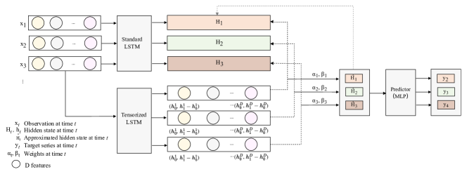
Figure 1: Proposed DeLELSTM model Framework.

3.2.1 Standard LSTM

The standard LSTM is shown in Equation (1).

$$\mathbf{I}_{t}=\sigma({U}_{i}\mathbf{H}_{t-1}+{W}_{i}\mathbf{x}_{t}+\mathbf{B}_{i})$$ (1)

$$\mathbf{F}_{t}=\sigma({U}_{f}\mathbf{H}_{t-1}+{W}_{f}\mathbf{x}_{t}+\mathbf{B}_{f})$$

$$\mathbf{O}_{t}=\sigma({U}_{o}\mathbf{H}_{t-1}+{W}_{o}\mathbf{x}_{t}+\mathbf{B}_{o})$$

$$\mathbf{\tilde{C}}_{t}=\tanh({U}_{c}\mathbf{H_{t-1}}+{W}_{c}\mathbf{x}_{t}+\mathbf{B}_{c})$$

$$\mathbf{C}_{t}=\mathbf{F}_{t}\odot\mathbf{C}_{t-1}+\mathbf{I}_{t}\odot\mathbf{\tilde{C}}_{t}$$

$$\mathbf{H}_{t}=\mathbf{O}_{t}\odot\tanh(\mathbf{C}_{t})$$

where $\mathbf{x}_{t}\in\mathbb{R}^{D}$ is the new observations of $D$ variables at time $t$, $\mathbf{H}_{t}\in\mathbb{R}^{M}$ is the hidden state at time $t$ which encodes information from all input variables until time $t$. $M$ is the dimension of the hidden state. $\odot$ is the elementwise product.

3.2.2 Tensorized LSTM

The tensorized LSTM is used to explain and approximate the hidden state $\mathbf{H}_{t}$ and identify the contribution of each variable. Here, the tensorized LSTM can be considered as a set of parallel LSTMs, each of which processes a single variable series. The hidden state of the tensorized LSTM is a matrix, and each row of the hidden state incorporates information only from a particular variable. Equation (2) shows the tensorized LSTM.

$$\mathbf{i}_{t}=\sigma(\mathcal{U}_{i}\circledast\mathbf{h}_{t-1}+\mathcal{W}_{i}\circledast\mathbf{x}_{t}+\mathbf{b_{i}})$$ (2)

$$\mathbf{f}_{t}=\sigma(\mathcal{U}_{f}\circledast\mathbf{h}_{t-1}+\mathcal{W}_{f}\circledast\mathbf{x}_{t}+\mathbf{b_{f}})$$

$$\mathbf{o}_{t}=\sigma(\mathcal{U}_{o}\circledast\mathbf{h}_{t-1}+\mathcal{W}_{o}\circledast\mathbf{x}_{t}+\mathbf{b_{o}})$$

$$\mathbf{\tilde{c}}_{t}=\tanh(\mathcal{U}_{c}\circledast\mathbf{h}_{t-1}+\mathcal{W}_{c}\circledast\mathbf{x}_{t}+\mathbf{b}_{c})$$

$$\mathbf{c}_{t}=\mathbf{f}_{t}\odot\mathbf{c}_{t-1}+\mathbf{i}_{t}\odot\mathbf{\tilde{c}}_{t}$$

$$\mathbf{h}_{t}=\mathbf{o}_{t}\odot\tanh(\mathbf{c}_{t})$$

where $\mathbf{h}_{t}=[\mathbf{h}_{t}^{1},\cdots,\mathbf{h}_{t}^{D}]^{T},\mathbf{h}_{t}\in\mathbb{R}^{D\times M}$,$\mathbf{h}_{t}^{d}\in\mathbb{R}^{M}$. The $\mathbf{h}_{t}^{d}$ is the hidden state vector specific to the $d$-th input variable at time $t$, and the $\mathbf{h}_{t}$ is the hidden state of all variables at time $t$. $\mathcal{U}_{c}=[\mathbf{u}_{c}^{1},\cdots,\mathbf{u}_{c}^{D}],~{}\mathcal{U}_{c}\in\mathbb{R}^{D\times M\times M},~{}\mathbf{u}_{c}^{d}\in\mathbb{R}^{M\times M}$, is the hidden-to-hidden transition. $\mathcal{W}_{c}=[\mathbf{w}_{c}^{1},\cdots,\mathbf{w}_{c}^{D}],~{}\mathcal{W}_{c}\in\mathbb{R}^{D\times M\times 1},~{}\mathbf{w}_{c}^{d}\in\mathbb{R}^{M\times 1}$, is the input-to-hidden transition. ($\mathcal{U}_{i},\mathcal{U}_{f},\mathcal{U}_{o}$), ( $\mathcal{W}_{i},\mathcal{W}_{f},\mathcal{W}_{o}$) have the same shapes as $\mathcal{U}_{c},\mathcal{W}_{c}$, respectively. $\circledast$ is the tensor-dot operation, which is defined as the product of two tensors along the $D$ axis, e.g., $\mathcal{U}_{c}\circledast\mathbf{h}_{t-1}=[\mathbf{u}_{c}^{1}\mathbf{h}_{t-1}^{1},\cdots,\mathbf{u}_{c}^{D}\mathbf{h}_{t-1}^{D}]^{T}$, $\mathbf{u}_{c}^{d}\mathbf{h}_{t-1}^{d}\in\mathbb{R}^{M}$. Such a design can guarantee that gates and memory cells are also matrices, and each row of these matrices only captures the information from a single variable.

3.2.3 Decomposition

$\mathbf{H}_{t}$ involves the information from previous steps and new input of all variables, so it is challenging to measure the influence of each variable, including the long-term effect from $\mathbf{H}_{t-1}$ and the instantaneous impact from $\mathbf{x}_{t}$.

Theoretically, each row of $\mathbf{h}_{t-1}$ corresponds to the information belonging to a particular variable until time $t-1$. Each row of $\Delta\mathbf{h}_{t}$ represents a single variable’s new information of time $t$, We propose to decompose $\mathbf{H}_{t}$ as a linear combination of $\mathbf{h}_{t-1}$ and $\Delta\mathbf{h}_{t}$, so that we can obtain each variable’s instantaneous influence and long-term impact.

Specifically, we approximate $\mathbf{H}_{t}$ using Equation (3):

$$\mathbf{H}_{t}\approx\sum_{i=1}^{D}(\alpha_{t}^{i}\mathbf{h}_{t-1}^{i}+\beta_{t}^{i}(\mathbf{h}_{t}^{i}-\mathbf{h}_{t-1}^{i}))$$ (3)

$$=\mathbf{h}_{t-1}^{T}\boldsymbol{\alpha}_{t}+(\mathbf{h}_{t}-\mathbf{h}_{t-1})^{T}\boldsymbol{\beta}_{t}$$

This approximation is minimised following a least squares criterion, which has a well-known solution, $\hat{\boldsymbol{\alpha}}_{t}$, $\hat{\boldsymbol{\beta}}_{t}$, and corresponding optimal approximation $\hat{\mathbf{H}}_{t}$. Here, we use $\hat{\mathbf{H}}_{t}$ to get the prediction of target $y_{t+1}$ and compute the hidden state $\mathbf{H}_{t+1}$.

3.3 Learning to Interpret

To get the immediate impact and the long-term effect of each variable, we derive significance from the magnitude of linear approximation weights rather than only focusing on the largest values. We first take the absolute value of $\hat{\boldsymbol{\alpha}}_{t}$, $\hat{\boldsymbol{\beta}}_{t}$ and get $\tilde{\boldsymbol{\alpha}}_{t}$, $\tilde{\boldsymbol{\beta}}_{t}$ after normalizing weights at each time step. Then, we propose several measures to interpret the prediction model for real-time series forecasting.

Definition 1.

The instantaneous importance of the d-th variable at time t, $In_{t}^{d}$, is defined as the Equation (4), the ratio of $\tilde{\beta}_{t}^{d}$ and $(\tilde{\alpha}_{t}^{d}+\tilde{\beta}_{t}^{d})$. Accordingly, the long-term effect of the d-th variable at time t is $1-In_{t}^{d}$.

$$In_{t}^{d}=\frac{\tilde{\beta}_{t}^{d}}{(\tilde{\alpha}_{t}^{d}+\tilde{\beta}_{t}^{d})}$$ (4)

$In_{t}^{d}$ can help us figure out which is more important: past information until time $t-1$ versus current data at time $t$ of the $d$-th variable. If $In_{t}^{d}$ is close to 1, we can know that the past information of the variable $d$ has little impact on the prediction; in other words, it has no long-term effect.

Definition 2.

The global importance of the d-th variable at time T, $Gl_{T}^{d}$, is defined as the Equation (5), which considers both the immediate impact and long-term impact of the d-th variable.

$$Gl_{T}^{d}=\frac{1}{T}\sum_{t=1}^{T}\sqrt{(\tilde{\alpha}_{t}^{d}{}^{2}+\tilde{\beta}_{t}^{d}{}^{2})}$$ (5)

The global importance of each variable can help us identify the important variables in general. Further, we can also get the dynamic shift in a variable’s weight by considering $\sqrt{(\tilde{\alpha}_{t}^{d}{}^{2}+\tilde{\beta}_{t}^{d}{}^{2})}$ over time, which we use to provide further model interpretability.

Algorithm 1 summarizes the proposed procedure.

Algorithm 1 The Training Process of DeLELSTM

Input:Time series $\mathbf{X}_{1:T}$, where $T$ is the max time length;
Set: $\mathbf{H}_{t}=\mathbf{H}_{0}$, $\mathbf{h}_{t}=\mathbf{h}_{0}$
Output: $\boldsymbol{\alpha}_{1:T}$, $\boldsymbol{\beta}_{1:T}$, $\mathbf{y}_{2:T+1}$

1:  for $t=1$ to $T$ do

2:     $\mathbf{H}_{t}$=standard LSTM($\mathbf{x}_{t}$, $\mathbf{H}_{t-1}$);

3:     $\mathbf{h}_{t}$=Tensorized LSTM($\mathbf{x}_{t}$, $\mathbf{h}_{t-1}$);

4:     $\Delta\mathbf{h}_{t}=\mathbf{h}_{t}-\mathbf{h}_{t-1}$;% Compute the dynamic change of hidden state $\mathbf{h}_{t}$ from $t-1$ to $t$

5:     $(\boldsymbol{\alpha}_{t},\boldsymbol{\beta}_{t})$=Least Square$(\mathbf{H}_{t},\mathbf{h}_{t-1},\Delta\mathbf{h}_{t})$;% Compute the optimal solution of $(\boldsymbol{\alpha}_{t},\boldsymbol{\beta}_{t})$ using Leaset Square

6:     $\hat{\mathbf{H}}_{t}=(\mathbf{h}_{t-1})^{T}\boldsymbol{\alpha}_{t}+(\Delta\mathbf{h}_{t})^{T}\boldsymbol{\beta}_{t}$% Compute the approximated hidden state $\hat{\mathbf{H}}_{t}$

7:     $\hat{y}_{t+1}$=MLP($\hat{\mathbf{H}}_{t})$

8:  end for

9:  return $\boldsymbol{\alpha}_{1:T}$, $\boldsymbol{\beta}_{1:T}$, $\mathbf{y}_{2:T+1}$

4 Experiment

In this section, we describe our experiments to evaluate the prediction performance and the interpretation ability of our proposed model .

4.1 Datasets

We used three publicly available real-world multivariate time series datasets covering meteorology, energy, and finance fields.

PM2.5 [27]: It contains hourly PM2.5 data and the associated meteorological measurements in Beijing from 2010.1.1 to 2014.12.31. PM2.5 is the target series. Aside from PM2.5 values, the meteorological variables include dew point, temperature, pressure, wind direction, wind speed, hours of snow, and hours of rain. Given the measurements, the task is to forecast PM2.5 each hour within a day. For example, using the data before 2:00 predicts PM2.5 at 2:00; using the data before 3:00 predict its value at 3:00, etc.

Electricity [28]: It records the time series of electricity consumption in the US, from 2017.10.11 to 2020.6.24. The consumption is chosen as the target series sampled hourly. The other 15 time series are exogenous factors, including max temperature, min temperature, visibility, etc. Similarly to PM2.5, our task is also to forecast consumption each hour of the day.

Exchange [29]: It is the collection of the daily exchange rates of eight foreign countries, including Australia, British, Canada, Switzerland, China, Japan, New Zealand, and Singapore, ranging from 1990 to 2016. We consider the time series of 30 days as a sample for this task. The Singapore exchange is taken as the target series, and we aim to predict the exchange rate of Singapore each day of a month.

4.2 Baseline Methods and Evaluation Setup

We evaluate the prediction performance of DeLELSTM with several baseline models as follows:

LSTM:[5]: LSTM network with one hidden layer is used to learn an encoding from multivariate time series data and make predictions at each time step. The prediction performance is also used as the basis for other models.

RETAIN:[25]: RETAIN is a two-level neural attention model for sequential data that can recognize the influential events and relevant characteristics within these events.

IMV-LSTM:[7]:IMV-LSTM explores the structure of LSTM network to learn variable-wise hidden states and separate the contribution of variables to the prediction. With hidden states, a mixture attention mechanism is explored to model the generative process of the target. It has two realizations of IMV-LSTM, i.e., IMV-Full and IMV-Tensor. We consider both versions.

We implemented the proposed model and deep learning baseline methods with Pytorch. We used Adam[30] optimizer. We conduct the grid search to select optimal parameters. The batch size is selected in $\{32,64,128\}$. Learning rate is searched in $\{0.05,0.01,0.001\}$. The size of the hidden states is selected in $\{32,64,128\}$. We train the models using $75\%$ of the samples, and $15\%$ of the samples are for validation. The remaining $10\%$ is used as the test set. We repeat the experiment five times and report the average performance with standard deviation.

We consider three metrics to measure the prediction performance, i.e., RMSE, MAE, and MAPE. RMSE is defined as $RMSE=\sqrt{\sum_{n}(y_{n}-\hat{y}_{n})^{2}/N}$. MAE is defined as $MAE=\sum_{n}\|y_{n}-\hat{y}_{n}\|/N$. MAPE is defined as $MAPE=\sum_{n}(\lvert\hat{y}_{n}-y_{n}\rvert/\lvert y_{n}\rvert)/N\times 100\%$, where $\hat{y}_{n}$ is the predicted value, and ${y}_{n}$ is the true value.

4.3 Prediction Performance

We compared the proposed DeLELSTM with four baseline models on real-time series forecasting and reported the results in Table 1. As shown in Table 1, among the attention-based models, the performance of RETAIN is better than IMV-LSTM in most cases. The IMV-Full is better than IMV-Tensor. Our proposed model presents comparable performance and obtains the best performance in electricity consumption prediction, indicating that our decomposition-based linear explainable model can still guarantee the prediction performance, while capturing the instantaneous and long-term effects and providing transparent and clear interpretation.

Dataset	Metric	LSTM	RETAIN	IMV-Full	IMV-Tensor	DeLELSTM
Electricity	RMSE	5.1049±6.3693	2.6685±0.2622	2.0284±0.1001	2.6069±0.9455	1.7247±0.0370
	MAE	3.9574±5.3274	2.0000±0.2136	1.4085±0.0899	1.7526±0.6754	1.1025±0.0128
	MAPE	6.49% ± 8.84%	3.21% ± 0.36%	2.28% ± 0.17%	2.74% ± 1.04%	1.69%±0.02%
PM2.5	RMSE	26.566 ± 0.152	24.913 ± 0.177	28.465 ± 0.264	28.866 ± 0.277	26.612 ± 0.470
	MAE	13.466 ± 0.098	13.402 ± 0.089	14.087 ± 0.266	14.480 ± 0.164	13.553 ± 0.168
	MAPE	22.47%±0.83%	21.23%±0.42%	25.21%±1.63%	26.67%±1.64%	22.16%±0.98%
Exchange	RMSE	0.0026±9.7e-06	0.0025±9.4e-06	0.0026±5.0e-06	0.0026±4.6e-06	0.0023±2.7e-05
	MAE	0.0015±3.8e-06	0.0015±1.0e-05	0.0015±5.5e-06	0.0015±3.1e-06	0.0015±1.5e-05
	MAPE	0.23%±5.5e-06	0.23% ±1.6e-05	0.22% ±3.2e-04	0.23% ±5.7e-06	0.23% ±2.3e-05

Table 1: Performance (±standard deviation) of baseline and proposed models

4.4 Interpretation

In this subsection, we depict three case studies designed to evaluate the effectiveness of DeLELSTM in providing insightful explanations of its forecasting. In particular, we qualitatively analyze the immediate and long-term impact of each variable identified by the defined measurement $ln_{t}^{d}$ and $1-ln_{t}^{d}$. We also report the meaningful variables at each time step and overall according to the defined measurement $Gl_{T}^{d}$.

4.4.1 Case Study I: Electricity Data

Predicting real-time electricity consumption accurately is quite important for electric power providers, so that they can more precisely manage resources for energy generation to maximize resource utilization, cut costs, and advance the development of smart grids. Figure 2 shows how the long-term and instantaneous (short-term) impacts change throughout the day. Here, we depict the change of the top 10 features, ordered by their overall importance for predicting electricity consumption. We can observe that compared with the short-term effects, the long-term information of most features is vital when people are sleeping and not engaged in other activities, and gradually diminishes importance during the daytime. On the other hand, the long-term effects of WindChill are important for electricity prediction.

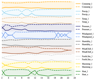
Figure 2: Electricity Long (l)/Short (s) term effects evolving over time (24h)

Figure 3 depicts the dynamic change of variable importance for the electricity consumption forecast. It is seen that the electricity consumption itself has an evident auto-correlation and contributes more to the prediction. In addition, as evening approaches, pressure and precipitation become more critical. While the temperature becomes important for electricity consumption at noon, because the temperature at noon tends to be high, people need to switch on the air-conditioner to have a comfortable environment. It is a primary reason that affects electricity consumption at noon. In general, variables consumption, precipitation, temperature, pressure, wind speed and humidity are highly ranked by DeLELSTM.

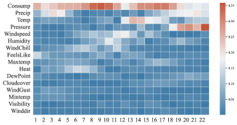
Figure 3: Electricity variable importance.

4.4.2 Case Study II: PM2.5 Data

PM2.5 is fine inhalable particles, with diameters that are generally 2.5 micrometers and smaller. Exposure to such fine particles has been linked to early death from heart and lung disease [31]. Understanding influential variables and forecasting PM2.5 accurately are necessary so that people can avoid going outside on time with high PM2.5 levels. We report the long-term and short-term effects of each variable during the day in Figure 4.

As shown in Figure 4, the impact of prior PM2.5 information is more significant than that of recent fresh information for real-time forecasting PM2.5 in a day. It indicates that PM2.5 always has long-term effects; we should utilize both past and current data of PM2.5. On the other hand, for other variables, such as dew point (DEWP), hours of snow(IS), temperature (TEMP), and the hours of rain (IR), the past information is only helpful before 6:00 am. After that, the ratio of instantaneous influence occupies almost $99\%$ for predicting PM2.5 in the next hour, showing little long-term effect. Therefore, we can conclude that it is sufficient to see the current data of these variables for forecasting PM2.5 during the daytime. One possible reason is that the natural environment has a significant impact on PM2.5 changes when there is less human activity and less pollution released at night, but human activity plays an important role during the day, so the long-term effects of these meteorological variables are lost.

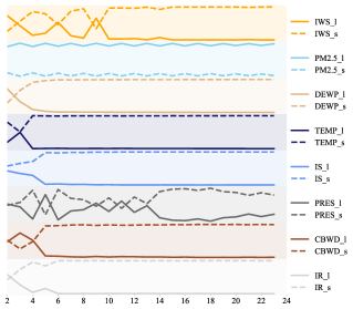
Figure 4: PM2.5 Long (l)/Short (s) term effects evolving over time (24h).

Figure 5 shows the dynamic change of variable importance considering the long-term effect and instantaneous influence. As shown in Figure 5, in the early morning, the PM2.5 itself contributes more to predict PM2.5 in the next hour. In the daytime, the wind speed, dew point, temperature, all take on greater significance. Taking into account all time steps, the top four important variables are the wind speed, PM2.5, the dew point, and the temperature. According to [32], wind speed has a significant impact on the amount of such inhalable particles transported and dispersion between Beijing and its surrounding areas. In addition, [27] also conclude that dew point and temperature are critical factors for PM2.5 prediction. Therefore, our variable importance is in line with the domain knowledge.

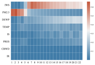
Figure 5: PM2.5 variable importance.

4.4.3 Case Study III: Exchange Data

Investors need to be very aware of changes in foreign exchange rates. These changes greatly impact the returns on foreign investments. As a result, if the exchange rate can be predicted with accuracy, investors could improve the timing of their foreign investments and earn higher returns. The long-term and short-term effects evolving over time for predicting Singapore’s exchange rate on the next day is shown in Figure 6. The exchange rates of Japan and Switzerland have both an immediate and long-term effects. Nevertheless, for other countries, the instantaneous influence is gradually increasing compared with the long-term effect.

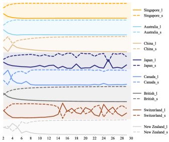
Figure 6: Exchange Long (l)/Short (s) term effects evolving over time (30 days).

Figure 7 displays the variable importance changing over time. Singapore has the biggest influence on predicting Singapore’s exchange rate on the next day, followed by Australia, China, and Japan.

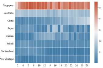
Figure 7: Exchange variable importance.

In summary, three case studies demonstrate that our proposed DeLELSTM can not only provide a transparent and clear explanation but also be able to distinguish the instantaneous influence and long-term effect of each variable. These explanations aid us in better understanding the data and building models for time series prediction.

4.5 Baseline Comparisons

In this subsection, we compare the interpretation results of the three baseline models, i.e., RETAIN, IMV-Full, and IMV-Tensor. Due to the page limitation, we show the variable importance at each time of three models in the supplementary.

As shown in Figure 1,2,3 in the supplementary¹, we can observe that the interpretable models based on the attention mechanism give the variable importance always the same at most of the time points. In addition, except for the most important variables identified by the models, it is hard for them to distinguish the importance of the other variables. The reason might be the hidden state representations are similar across time steps [9].

To further evaluate the sufficiency of our explanation model, we retain the top 50% of features identified by each explainable model, and then feed them into the LSTM of the same architecture to obtain the prediction results. Table 2 shows the prediction results on the electricity consumption task. We can observe that features selected by our model can obtain better performance.

Model	RMSE	MAE	MAPE
DeLELSTM	1.677±0.022	1.116±0.019	1.746%±0.038%
IMV-Full	5.332±1.232	3.964±0.959	6.264%±1.418%
IMV-Tensor	1.686±0.020	1.130±0.022	1.776%±0.046%
RETAIN	1.695±0.027	1.146±0.025	1.807%±0.046%

Table 2: Performance based on top 50% important variables

Compared with these baseline models, our proposed model is able to identify the dynamic impacts of variables on the prediction over time, and distinguish the instantaneous influence and the long-term effects of each variable.

5 Conclusion

Explaining the time series forecasting model is of significance, especially in high-stakes applications. In this work, we propose DeLELSTM, a decomposition-based linear explainable LSTM, to improve the interpretability of LSTM. Specifically, DeLELSTM decomposes the hidden states into the linear combination of the past information and the new information of each variable so that it can capture the instantaneous influence and long-term effects. The utilization of linear regression also guarantees that the explanations are transparent and clear. The experimental results on three real datasets demonstrate the effectiveness of DeLELSTM compared with baseline models. The case studies show that the explanations made by DeLELSTM are in line with domain knowledge.

One limitation of this work is that the contributions to the prediction are for individual variables, ignoring the complex interactions between variables, which is common in real life. We keep this challenging task as our future work.

References

- [1] Yue Wu, José Miguel Hernández-Lobato, and Ghahramani Zoubin. Dynamic covariance models for multivariate financial time series. In International Conference on Machine Learning, pages 558–566. PMLR, 2013.
- [2] Prithwish Chakraborty, Manish Marwah, Martin Arlitt, and Naren Ramakrishnan. Fine-grained photovoltaic output prediction using a bayesian ensemble. Proceedings of the AAAI Conference on Artificial Intelligence, 26(1):274–280, Sep. 2021.
- [3] Jian Qi Wang, Yu Du, and Jing Wang. Lstm based long-term energy consumption prediction with periodicity. Energy, 197:117197, 2020.
- [4] Yuan Zhang. Attain: Attention-based time-aware lstm networks for disease progression modeling. In In Proceedings of the 28th International Joint Conference on Artificial Intelligence (IJCAI-2019), pp. 4369-4375, Macao, China., 2019.
- [5] Sepp Hochreiter and Jürgen Schmidhuber. Long short-term memory. Neural computation, 9(8):1735–1780, 1997.
- [6] Kyunghyun Cho, Bart Van Merriënboer, Caglar Gulcehre, Dzmitry Bahdanau, Fethi Bougares, Holger Schwenk, and Yoshua Bengio. Learning phrase representations using rnn encoder-decoder for statistical machine translation. arXiv preprint arXiv:1406.1078, 2014.
- [7] Tian Guo, Tao Lin, and Nino Antulov-Fantulin. Exploring interpretable lstm neural networks over multi-variable data. In International conference on machine learning, pages 2494–2504. PMLR, 2019.
- [8] Aria Masoomi, Davin Hill, Zhonghui Xu, Craig P Hersh, Edwin K Silverman, Peter J Castaldi, Stratis Ioannidis, and Jennifer Dy. Explanations of black-box models based on directional feature interactions. In International Conference on Learning Representations, 2021.
- [9] Akash Kumar Mohankumar, Preksha Nema, Sharan Narasimhan, Mitesh M Khapra, Balaji Vasan Srinivasan, and Balaraman Ravindran. Towards transparent and explainable attention models. arXiv preprint arXiv:2004.14243, 2020.
- [10] Michael Tsang, Sirisha Rambhatla, and Yan Liu. How does this interaction affect me? interpretable attribution for feature interactions. Advances in neural information processing systems, 33:6147–6159, 2020.
- [11] Sana Tonekaboni, Shalmali Joshi, Kieran Campbell, David K Duvenaud, and Anna Goldenberg. What went wrong and when? instance-wise feature importance for time-series black-box models. Advances in Neural Information Processing Systems, 33:799–809, 2020.
- [12] Thomas Rojat, Raphaël Puget, David Filliat, Javier Del Ser, Rodolphe Gelin, and Natalia Díaz-Rodríguez. Explainable artificial intelligence (xai) on timeseries data: A survey. arXiv preprint arXiv:2104.00950, 2021.
- [13] Tsung-Yu Hsieh, Suhang Wang, Yiwei Sun, and Vasant Honavar. Explainable multivariate time series classification: a deep neural network which learns to attend to important variables as well as time intervals. In Proceedings of the 14th ACM international conference on web search and data mining, pages 607–615, 2021.
- [14] Xiaofei Sun, Diyi Yang, Xiaoya Li, Tianwei Zhang, Yuxian Meng, Han Qiu, Guoyin Wang, Eduard Hovy, and Jiwei Li. Interpreting deep learning models in natural language processing: A review. arXiv preprint arXiv:2110.10470, 2021.
- [15] Sofia Serrano and Noah A Smith. Is attention interpretable? arXiv preprint arXiv:1906.03731, 2019.
- [16] Zhen He, Shaobing Gao, Liang Xiao, Daxue Liu, Hangen He, and David Barber. Wider and deeper, cheaper and faster: Tensorized lstms for sequence learning. Advances in neural information processing systems, 30, 2017.
- [17] Weiping Ding, Mohamed Abdel-Basset, Hossam Hawash, and Ahmed M Ali. Explainability of artificial intelligence methods, applications and challenges: A comprehensive survey. Information Sciences, 2022.
- [18] Marco Ancona, Enea Ceolini, Cengiz Öztireli, and Markus Gross. Towards better understanding of gradient-based attribution methods for deep neural networks. arXiv preprint arXiv:1711.06104, 2017.
- [19] Avanti Shrikumar, Peyton Greenside, and Anshul Kundaje. Learning important features through propagating activation differences. In International conference on machine learning, pages 3145–3153. PMLR, 2017.
- [20] Mukund Sundararajan, Ankur Taly, and Qiqi Yan. Axiomatic attribution for deep networks. In International conference on machine learning, pages 3319–3328. PMLR, 2017.
- [21] Yinchong Yang, Volker Tresp, Marius Wunderle, and Peter A Fasching. Explaining therapy predictions with layer-wise relevance propagation in neural networks. In 2018 IEEE International Conference on Healthcare Informatics (ICHI), pages 152–162. IEEE, 2018.
- [22] Piotr Dabkowski and Yarin Gal. Real time image saliency for black box classifiers. Advances in neural information processing systems, 30, 2017.
- [23] Ruth C Fong and Andrea Vedaldi. Interpretable explanations of black boxes by meaningful perturbation. In Proceedings of the IEEE international conference on computer vision, pages 3429–3437, 2017.
- [24] Mattia Rigotti, Christoph Miksovic, Ioana Giurgiu, Thomas Gschwind, and Paolo Scotton. Attention-based interpretability with concept transformers. In International Conference on Learning Representations, 2021.
- [25] Edward Choi, Mohammad Taha Bahadori, Jimeng Sun, Joshua Kulas, Andy Schuetz, and Walter Stewart. Retain: An interpretable predictive model for healthcare using reverse time attention mechanism. Advances in neural information processing systems, 29, 2016.
- [26] Sarthak Jain and Byron C Wallace. Attention is not explanation. arXiv preprint arXiv:1902.10186, 2019.
- [27] Xuan Liang, Tao Zou, Bin Guo, Shuo Li, Haozhe Zhang, Shuyi Zhang, Hui Huang, and Song Xi Chen. Assessing beijing’s pm2. 5 pollution: severity, weather impact, apec and winter heating. Proceedings of the Royal Society A: Mathematical, Physical and Engineering Sciences, 471(2182):20150257, 2015.
- [28] Penglei Gao, Xi Yang, Kaizhu Huang, Rui Zhang, and John Yannis Goulermas. Explainable tensorized neural ordinary differential equations for arbitrary-step time series prediction. IEEE Transactions on Knowledge and Data Engineering, 2022.
- [29] Guokun Lai, Wei-Cheng Chang, Yiming Yang, and Hanxiao Liu. Modeling long-and short-term temporal patterns with deep neural networks. In The 41st international ACM SIGIR conference on research & development in information retrieval, pages 95–104, 2018.
- [30] Diederik P Kingma and Jimmy Ba. Adam: A method for stochastic optimization. arXiv preprint arXiv:1412.6980, 2014.
- [31] Meredith Franklin, Petros Koutrakis, and Joel Schwartz. The role of particle composition on the association between pm2. 5 and mortality. Epidemiology (Cambridge, Mass.), 19(5):680, 2008.
- [32] Wei-wei Pu, Xiu-juan Zhao, Xiao-ling Zhang, and Zhi-qiang Ma. Effect of meteorological factors on pm2. 5 during july to september of beijing. Procedia Earth and Planetary Science, 2:272–277, 2011.