Causally Sound Priors for Binary Experiments

Abstract

We introduce the BREASE framework for the Bayesian analysis of randomized controlled trials with a binary treatment and a binary outcome. Approaching the problem from a causal inference perspective, we propose parameterizing the likelihood in terms of the baseline risk, efficacy, and adverse side effects of the treatment, along with a flexible, yet intuitive and tractable jointly independent beta prior distribution on these parameters, which we show to be a generalization of the Dirichlet prior for the joint distribution of potential outcomes. Our approach has a number of desirable characteristics when compared to current mainstream alternatives: (i) it naturally induces prior dependence between expected outcomes in the treatment and control groups; (ii) as the baseline risk, efficacy and risk of adverse side effects are quantities commonly present in the clinicians’ vocabulary, the hyperparameters of the prior are directly interpretable, thus facilitating the elicitation of prior knowledge and sensitivity analysis; and (iii) we provide analytical formulae for the marginal likelihood, Bayes factor, and other posterior quantities, as well as exact posterior sampling via simulation, in cases where traditional MCMC fails. Empirical examples demonstrate the utility of our methods for estimation, hypothesis testing, and sensitivity analysis of treatment effects.

1 Introduction

Randomized controlled trials (RCTs) form the cornerstone of scientific research across numerous disciplines. In their most basic form, these trials compare the occurrence of an adverse (or favorable) outcome between treatment and control groups. This is particularly evident in a drug or vaccine trial, in which the efficacy of an intervention is established by comparing the number of individuals who die or develop a disease in each arm of the study. We refer to this type of study design as a “binary experiment,” wherein each participant is subjected to either a treatment or a control condition (a binary exposure), and we observe either the presence or absence of the adverse effect of interest (a binary outcome).

If participants of the trial are independent draws from a common (super-)population, statistical inference in binary experiments amounts to what is perhaps the simplest of tasks in statistics—the comparison of two binomial proportions. Indeed, from a Bayesian perspective, inference on the parameter of a binomial distribution dates back to at least as early as the origins of Bayesian inference itself, as evidenced by the seminal works of [67] and [68]. The task comprises specifying a joint prior distribution for both binomial parameters, and computing the posterior distribution (or Bayes factors) of (relevant contrasts of) such parameters (e.g., the risk difference, or the risk ratio). Yet, perhaps surprisingly, despite this long tradition, their widespread occurrence in the sciences, and the apparent simplicity of the inferential task, mainstream approaches for prior specification in the analysis of binary experiments have several shortcomings.

As reviewed in [110] and [129] (and also evident from perusing popular textbooks) the two predominant approaches for the Bayesian analysis of binary experiments consist of: (i) assigning independent beta priors to each of the binomial proportions, which are conjugate priors to the (also independent) binomials comprising the likelihood; and, (ii) what is essentially a logistic regression, i.e., applying a logit transformation to the binomial proportions, and assigning Gaussian priors to the average log odds and the log odds ratio. For all their popularity, these two approaches are unsatisfactory in several ways. For example, in the first case, the assumption of prior independence of the two proportions is often not credible—e.g., in most settings, one expects that learning about the mortality rate in the control group should inform our beliefs about the mortality rate in the treatment group. Moreover, while the logit approach addresses the problem of prior dependence, it does so at the sacrifice of clarity and interpretation—odds ratios are notoriously difficult to understand [103], thus hindering the utility of this approach for prior elicitation and sensitivity analysis.

In this paper we demonstrate how causal logic can be used to address these challenges. Approaching the problem from a causal inference perspective, we first propose parameterizing the likelihood in terms of three clinically meaningful counterfactual quantities: the baseline risk, efficacy, and risk of adverse side effects (BREASE) of the intervention. We then propose a flexible, yet intuitive and tractable jointly independent beta prior distribution on these parameters, which we show to be a generalization of the Dirichlet prior on the joint distribution of potential outcomes. Our approach has a number of desirable characteristics: (i) it naturally induces prior dependence between the two binomial proportions of the treatment and control arms of the study; (ii) as the baseline risk, efficacy and risk of adverse side effects are quantities familiar to clinicians, the hyperparameters of the prior are directly interpretable, thus facilitating the elicitation of prior knowledge and sensitivity analysis; and (iii) we derive analytical formulae for the marginal likelihood, Bayes factor, and other posterior quantities, as well as exact posterior sampling via simulation, in cases where traditional MCMC fails.

Related literature.

When framed in the language of potential outcomes, causal inference can be seen as a missing data problem. Thus, our analysis is most closely related to the literature on contingency tables with missing or incomplete observations on certain cell counts. In fact, our proposed prior can be shown to induce a generalized Dirichlet distribution on the joint distribution of potential outcomes. This distribution has been studied in the 1970s and 1980s [74, 77, 87, 91], though mostly in the context of survey sampling. Perhaps due to the intractability of the integrals, the difficulty in interpretation of the original generalized Dirichlet parameterization, and the missing connection to formal causal inference, this prior has received little to no attention in the analysis of binary experiments. Our analysis shows that the generalized Dirichlet distribution emerges naturally from the causal formulation of the problem, that the parameters of the distribution can be cast in intuitive clinical terms, and that statistical inference is manageable, with exact posterior sampling and analytical formulae for Bayes factors, which we derive in this paper.

Outline of the paper.

Section 2 introduces the statistical setup for the analysis of binary experiments and reviews existing methods for Bayesian inference in this setting. Section 3 introduces our proposal. It also derives key results for implementation, such as analytical formulae for the marginal likelihood and algorithms for exact posterior sampling. Section 4 demonstrates the utility of our method in three empirical examples. Section 5 concludes the paper, and suggests possible extensions for future research. Code to replicate our analysis is available at https://github.com/njirons/causally-sound.

2 Preliminaries

In this section we set notation, the statistical setup, and briefly review the two main approaches currently used for the Bayesian analysis of binary experiments—the independent beta and logit transformation approaches. We also briefly introduce the response type parameterization of the joint distribution of potential outcomes, which is an important stepping stone for understanding our proposal.

2.1 Potential outcomes

Our analysis is situated within the potential outcomes framework of causal inference [93, 79]. Let $N$ denote the total number of participants in the study, $Z_{i}$ a binary treatment indicator and $Y_{i}$ a binary outcome indicator for subject $i\in\{1,\ldots,N\}$. We denote by $Y_{i}(z)$ the potential outcome of subject $i$ under the experimental condition $Z_{i}=z$, where $z=0$ indicates the control and $z=1$ the treatment condition. Under the standard consistency assumption, we have that the observed outcome of subject $i$ equals the potential outcome associated to the experimental condition that subject $i$ has actually received, i.e., $Y_{i}=Y_{i}(Z_{i})$. Throughout the paper, we adopt the convention that $Y_{i}=1$ denotes an adverse outcome, such as death or the contraction of a disease. We take a super-population perspective, and assume that subjects are independent and identically distributed (i.i.d.) draws from a common population. We assume complete randomization, which implies ignorability of the treatment assignment, $\{Y_{i}(1),Y_{i}(0)\}\perp\!\!\!\perp Z_{i}$.

2.2 Marginal parameterization

When subjects are independently drawn from a common super-population and the treatment is assigned at random, it follows that the observed counts of adverse outcomes in each treatment arm,

$$y_{0}=\sum_{i:Z_{i}=0}Y_{i},\qquad y_{1}=\sum_{i:Z_{i}=1}Y_{i},$$

follow independent binomial distributions:

$$y_{0} \sim\text{Binomial}(N_{0},\theta_{0})\quad\perp\!\!\!\perp\quad y_{1}\sim\text{Binomial}(N_{1},\theta_{1}),$$

where here, $\theta_{1}=\mathbb{P}(Y_{i}(1)=1)$, $N_{1}=\sum_{i}Z_{i}$ denote the probability of an adverse outcome and the sample size of the treatment group, and $\theta_{0}=\mathbb{P}(Y_{i}(0)=1)$, $N_{0}=N-N_{1}$ are the analogous quantities for the control group. We refer to the probabilities $\theta_{0}$ and $\theta_{1}$ as the baseline risk and risk of treatment, respectively.

This defines the likelihood under the marginal parameterization of a binary experiment—so called because the parameters $(\theta_{0},\theta_{1})$ are defined in terms of the marginal distribution of the potential outcomes $Y_{i}(0)$ and $Y_{i}(1)$:

$$L(\mathcal{D}|\theta_{0},\theta_{1})=\binom{N_{0}}{y_{0}}\theta_{0}^{y_{0}}(1-\theta_{0})^{N_{0}-y_{0}}\times\binom{N_{1}}{y_{1}}\theta_{1}^{y_{1}}(1-\theta_{1})^{N_{1}-y_{1}},$$ (2.1)

where hereafter we denote the observed data by $\mathcal{D}=(y_{0},y_{1},N_{0},N_{1})$. To determine the effect of treatment, if any, Bayesian inference is carried out using the posterior distribution of the parameters $(\theta_{0},\theta_{1})$, which requires specification of a prior distribution for $(\theta_{0},\theta_{1})$. There are two main parameterizations with accompanying priors currently in use, discussed extensively in [110] and [129]—these are the independent beta (IB) and logit transformation (LT) approaches, which we now discuss.

2.2.1 Independent beta (IB) approach

The independent beta (IB) approach [69] assigns the prior

$$\theta_{0}\sim\text{Beta}(a_{0},b_{0})\quad\perp\!\!\!\perp\quad\theta_{1}\sim\text{Beta}(a_{1},b_{1}),$$ (2.2)

for some hyperparameters $a_{0},b_{0},a_{1},b_{1}>0$. A common specification is $a_{0}=b_{0}=a_{1}=b_{1}=1$, which assigns a uniform distribution to $(\theta_{0},\theta_{1})$. This choice of flat priors is usually thought to encode ignorance of $(\theta_{0},\theta_{1})$ a priori, though it makes strong implicit assumptions as we discuss next. We refer to (2.2) as the $\text{IB}(a;b)$ prior, where $a=(a_{0},a_{1}),b=(b_{0},b_{1})$.

The main advantage of the IB approach is its simplicity. As the beta prior is conjugate to the binomial likelihood, estimation and posterior simulation can be carried out exactly without resorting to approximate sampling algorithms, such as MCMC. Furthermore, marginal likelihoods and Bayes factors, which are widely used for Bayesian hypothesis testing and can be difficult to calculate in general (usually requiring numerical approximation or estimation via posterior simulation), can be calculated analytically [98].

A significant drawback of the IB approach is the restrictive assumption of independence between $\theta_{0}$ and $\theta_{1}$. In most experimental settings, we would expect our knowledge about the risks in the control and treatment groups to be dependent. For example, if we known that the population prevalence of an infectious disease is approximately 1%, we would expect the prevalence of the disease among those receiving a vaccine to be concentrated around 1% or below, reflecting the common prior belief that it is unlikely that the vaccine would cause the disease. The IB prior fails to accommodate this natural dependence between risks in each arm of the trial. Furthermore, since independence in the prior and the likelihood implies independence a posteriori, this failure also extends to the posterior.

2.2.2 Logit Transformation (LT) approach

The logit transformation (LT) approach [94, 109, 129] reparameterizes the model in terms of the logit-transformed risks, by defining the parameters $(\beta,\psi)$ satisfying

$$\log\left(\frac{\theta_{0}}{1-\theta_{0}}\right)=\beta-\frac{\psi}{2},\qquad\log\left(\frac{\theta_{1}}{1-\theta_{1}}\right)=\beta+\frac{\psi}{2}.$$

Note this parameterization is equivalent to a logistic regression of the outcome on the treatment with the encoding $Z\in\{-1/2,1/2\}$ [127]. It then assigns an independent normal prior to $(\beta,\psi)$:

$$\beta\sim\text{Normal}(\mu_{\beta},\sigma_{\beta}^{2})\quad\perp\!\!\!\perp\quad\psi\sim\text{Normal}(\mu_{\psi},\sigma_{\psi}^{2}),$$ (2.3)

where $\mu=(\mu_{\beta},\mu_{\psi})$ and $\sigma=(\sigma_{\beta},\sigma_{\psi})>0$ are hyperparameters. This prior encodes correlation between $\theta_{0}$ and $\theta_{1}$ through their shared dependence on $\beta$ and $\psi$. We refer to (2.3) as the $\text{LT}(\mu;\sigma)$ prior. Figure 1 depicts probabilistic graphical models comparing the IB and LT parameterizations, as well as the other approaches we will introduce in this paper.

(a) Independent Beta

(b) Logit Transform

(c) Response Type

(d) BREASE

Figure 1: Probabilistic graphical models for different parameterizations and prior setups. Gray nodes denote observed variables, white nodes denote latent parameters, and double borders indicate that a node is a deterministic function of its parents. (a) Independent beta priors are placed directly on $\theta_{0}$ and $\theta_{1}$; (b) Independent Gaussian priors are placed on the log odds quantities $\beta$ and $\psi$; (c) A Dirichlet prior is placed on the response type probabilities $\mathbf{p}$; (d) Our proposal, independent beta priors are placed on $\theta_{0}$, $\eta_{e}$, and $\eta_{s}$. In all cases, the observed data depends only on $\theta_{0}$ and $\theta_{1}$.

While the LT approach induces prior dependence between $\theta_{0}$ and $\theta_{1}$, this comes at the cost of a less intuitive parameterization. Here $\beta$ is interpreted as the “grand log odds,” i.e, the average of the log odds across treatment arms, whereas $\psi$ is the log odds ratio. Odds ratios are notoriously difficult to understand, and thus reasoning about the plausible prior means and variances of log odds—two unbounded hyperparameters—is often challenging in practice. The LT approach also has other computational disadvantages relative to the IB prior. Unlike the IB approach, marginal likelihoods and Bayes factors for the LT approach are not available analytically, and posterior sampling must be carried out approximately.

2.3 Response type (RT) parameterization

The IB and LT approaches focus on the margins of the joint distribution of the potential outcomes $Y_{i}(0)$ and $Y_{i}(1)$. This focus is natural, because the observed data depends only upon the parameters $\theta_{0}$ and $\theta_{1}$. However, thinking in terms of their joint distribution reveals alternative ways of inducing prior dependence between these parameters. Specifically, the joint distribution of potential outcomes is fully characterized by four probabilities

$$p_{jk}=\mathbb{P}(Y_{i}(0)=j,Y_{i}(1)=k),\qquad j,k\in\{0,1\}.$$ (2.4)

The probabilities $\mathbf{p}=\{p_{jk}\}_{j,k\in\{0,1\}}$ describe the frequencies of the four possible response types in the population [76, 90]. These include: (i) the “doomed” $\{Y_{i}(0)=1,Y_{i}(1)=1\}$, for whom the adverse outcome occurs regardless of treatment; (ii) the “immune” $\{Y_{i}(0)=0,Y_{i}(1)=0\}$, for whom the adverse outcome does not occur regardless of treatment; (iii) the “preventive” $\{Y_{i}(0)=1,Y_{i}(1)=0\}$, for whom treatment prevents the adverse outcome; and, (iv) the “causal” $\{Y_{i}(0)=0,Y_{i}(1)=1\}$, for whom treatment causes the adverse outcome. Here $\theta_{0}$ and $\theta_{1}$, which satisfy $\theta_{0}=p_{10}+p_{11}$ and $\theta_{1}=p_{01}+p_{11}$, define the margins of Table 1.

	${Y_{i}(0)=0}$	${Y_{i}(0)=1}$	Row Sum
${Y_{i}(1)=0}$	$p_{00}=(1-\eta_{s})(1-\theta_{0})$	$p_{10}=\eta_{e}\theta_{0}$	$1-\theta_{1}$
${Y_{i}(1)=1}$	$p_{01}=\eta_{s}(1-\theta_{0})$	$p_{11}=(1-\eta_{e})\theta_{0}$	$\theta_{1}$
Column Sum	$1-\theta_{0}$	$\theta_{0}$

Table 1: $2\times 2$ contingency table of potential outcomes for a binary experiment. Only the margins of the table are identified from the observed data.

Whereas in the marginal parameterization, independence of the likelihood and prior imply that estimation of $\theta_{0}$ is only informed by data in the control group (and similarly for $\theta_{1}$), the response type (RT) parameterization intertwines the data from each arm of the study. The shared dependence of $\theta_{0}$ and $\theta_{1}$ on the response type proportions reveals the link between outcomes in the control and treated groups.

A Bayesian approach to modeling the response type probabilities $\mathbf{p}$ requires specification of a prior density supported on the probability simplex, making the Dirichlet distribution a natural candidate

$$\mathbf{p}=(p_{00},p_{10},p_{01},p_{11})\sim\text{Dirichlet}(a_{00},a_{10},a_{01},a_{11}),\qquad a_{00},a_{10},a_{01},a_{11}>0.$$ (2.5)

Indeed, priors of this type have been used in the analysis of partially identified quantities in randomized trials with non-compliance, such as in [101]. As we show next, the Dirichlet prior is a special case of our proposal, and our analysis not only extends it, but also clarifies its advantages and limitations as a means to induce the desired joint prior distribution on the two binomial proportions $(\theta_{0},\theta_{1})$.

3 The BREASE framework

In this section we introduce the BREASE framework for the analysis of binary experiments. We start by parameterizing the likelihood in terms of the baseline risk, efficacy, and risk of adverse side effects of the treatment. We then propose a jointly independent beta prior distributions on these three parameters, which we show to be a generalization of the Dirichlet prior on the response types. Our proposal has a number of advantages. From a statistical perspective, it induces dependence between the risks in the treatment and control groups, while also enabling exact posterior sampling, and marginal likelihood calculations. From a clinical perspective, this parameterization casts the model in terms of natural quantities appearing frequently in the clinician’s vocabulary, thereby facilitating interpretability, elicitation of prior knowledge, and sensitivity analyses.

3.1 Baseline risk, efficacy and adverse side effects

To make things concrete, suppose $Y_{i}=1$ denotes death. We define the efficacy of the treatment, $\eta_{e}$, as the probability that the treatment prevents the death of a patient that would have otherwise died without it:

$$\eta_{e}=\mathbb{P}(Y_{i}(1)=0|Y_{i}(0)=1).$$ (3.1)

Similarly, we define the risk of adverse side effects of the treatment, $\eta_{s}$, as the probability that the treatment causes the death of a patient that would have otherwise been healthy:

$$\eta_{s}=\mathbb{P}(Y_{i}(1)=1|Y_{i}(0)=0).$$ (3.2)

These quantities can be interpreted as probabilities of sufficient causation [107, 126], i.e., $\eta_{e}$ is the probability that treatment is sufficient to save or cure a patient, while $\eta_{s}$ is the probability that treatment is sufficient to kill or hurt a patient. They correspond directly to the counterfactual interpretation of what clinicians colloquially refer to as “efficacy” and “side effects” of a drug or vaccine. Indeed, not coincidentally, a commonly used measure in clinical trials called “efficacy”, defined as $1-\theta_{1}/\theta_{0}$, equals precisely $\eta_{e}$ under the assumption that treatment causes no harm ($\eta_{s}=0$).

Applying the law of total probability, we can decompose the risk of treatment in terms of the baseline risk, efficacy, and risk of adverse side effects (BREASE), as

$$\theta_{1}=(1-\eta_{e})\theta_{0}+\eta_{s}(1-\theta_{0}).$$ (3.3)

Table 1 shows how the response type probabilities $\mathbf{p}$ can be written as products of $\theta_{0}$, $\eta_{s}$, and $\eta_{e}$. As with the response type approach, this parameterization highlights the natural dependence between $\theta_{0}$ and $\theta_{1}$ that is nevertheless easy to miss without framing the problem in the language of potential outcomes. For example, note that $\theta_{0}$ and $\theta_{1}$ are functionally independent only under the strong assumption that $\eta_{e}=1-\eta_{s}$, i.e., the probability of treatment saving a patient is equal to the probability that it doesn’t kill one.

3.1.1 Likelihood

Plugging in (3.3), we can rewrite the likelihood (2.1) in terms of $(\theta_{0},\eta_{e},\eta_{s})$.

Theorem 1.

Under (2.1) and (3.1-3.3), the likelihood is

$$L(\mathcal{D}|\theta_{0},\eta_{e},\eta_{s}) =\binom{N_{0}}{y_{0}}\binom{N_{1}}{y_{1}}\sum_{j=0}^{y_{1}}\sum_{k=0}^{N_{1}-y_{1}}\binom{y_{1}}{j}\binom{N_{1}-y_{1}}{k}\times\theta_{0}^{y_{0}+j+k}(1-\theta_{0})^{N-(y_{0}+j+k)}$$

$$\quad\times\eta_{e}^{k}(1-\eta_{e})^{j}$$

$$\quad\times\eta_{s}^{y_{1}-j}(1-\eta_{s})^{N_{1}-y_{1}-k},\qquad(\theta_{0},\eta_{e},\eta_{s})\in[0,1]^{3}.$$ (3.4)

Theorem 1 follows from applying the binomial theorem twice. As the likelihood (3.4) is polynomial in $(\theta_{0},\eta_{e},\eta_{s})$, any prior distribution $\pi(\theta_{0},\eta_{e},\eta_{s})$ for which the moments can be explicitly calculated yields an analytical expression for the marginal likelihood. In particular, if

$$\pi(\theta_{0},\eta_{e},\eta_{s})\propto\theta_{0}^{\alpha_{0}-1}(1-\theta_{0})^{\beta_{0}-1}\times\eta_{e}^{\alpha_{e}-1}(1-\eta_{e})^{\beta_{e}-1}\times\eta_{s}^{\alpha_{s}-1}(1-\eta_{s})^{\beta_{s}-1}$$

is a product of independent beta distributions, as we will see in the next section, then the marginal likelihood is a weighted sum of beta function values. Furthermore, the posterior distribution $\pi(\theta_{0},\eta_{e},\eta_{s}|\mathcal{D})$ will be a mixture of independent beta distributions, from which we can sample exactly via simulation.

3.1.2 Partial identification and monotonicity

The parameters $\eta_{e}$ and $\eta_{s}$ are only partially identified by the observed data. That is, without further assumptions, we have the following bounds,

$$\max\left\{0,1-\frac{\theta_{1}}{\theta_{0}}\right\}\leq\eta_{e}\leq\min\left\{\frac{1-\theta_{1}}{\theta_{0}},1\right\},\quad\max\left\{0,\frac{\theta_{1}-\theta_{0}}{1-\theta_{0}}\right\}\leq\eta_{s}\leq\min\left\{\frac{\theta_{1}}{1-\theta_{0}},1\right\}.$$

Thus, as the sample size increases, the posterior distribution of $\eta_{s}$ and $\eta_{e}$ will not concentrate in a point—rather, it will remain spread over its partially identified region [118, 121]. Notice, however, that this does not affect the behavior of the posterior distribution of $(\theta_{0},\theta_{1})$. The BREASE parameterization thus explicitly separates the identified and partially identified parameters—$(\theta_{0},\theta_{1})$ and $(\eta_{e},\eta_{s})$, respectively. Even if interest does not lie in the counterfactual probabilities $(\eta_{s},\eta_{e})$ per se, assigning a prior to those quantities can be thought of as a causally principled way to specify a joint prior on the identified target parameters $(\theta_{0},\theta_{1})$.

Finally, a common assumption in the potential outcomes literature is called monotonicity, which states that the treatment does no harm. In our framework, this corresponds to the constraint $\eta_{s}=0$. This assumption is reasonable in many clinical settings. Under monotonicity, the efficacy of the treatment is in fact point identified, and given by $\eta_{e}=1-\theta_{1}/\theta_{0}$. The quantity $\theta_{1}/\theta_{0}$ is known as the risk ratio, and the quantity $1-\theta_{1}/\theta_{0}$ is indeed known as “efficacy” in the clinical trials literature. While the hard constraint $\eta_{s}=0$ may not be credible in some settings, if side effects are expected to be small, the BREASE approach allows one to instead place an informative prior on $\eta_{s}$.

3.2 Prior specification

Bayesian inference with the likelihood (3.4) requires specifying a prior distribution on three separate and variation independent probabilities, $(\theta_{0},\eta_{e},\eta_{s})$. We propose setting jointly independent beta prior distributions on these parameters:

$$\theta_{0}\sim\text{Beta}^{*}(\mu_{0},n_{0})\quad\perp\!\!\!\perp\quad\eta_{e}\sim\text{Beta}^{*}(\mu_{e},n_{e})\quad\perp\!\!\!\perp\quad\eta_{s}\sim\text{Beta}^{*}(\mu_{s},n_{s}),$$ (3.5)

where here $\text{Beta}^{*}(\mu,n)$ denotes a $\text{Beta}(a,b)$ distribution, with mean $\mu=a/(a+b)$ and prior “sample size” $n=a+b$. We refer to (3.5) as the $\text{BREASE}(\mu;n)$ prior, where $\mu=(\mu_{0},\mu_{e},\mu_{s})$, $n=(n_{0},n_{e},n_{s})$.

Since (3.5) defines a jointly independent beta prior on $(\theta_{0},\eta_{e},\eta_{s})$, the discussion in Section 3.1.1 applies. In particular, the posterior of $(\theta_{0},\eta_{e},\eta_{s})$ is a mixture of independent betas, which permits exact sampling via simulation, and the marginal likelihood is available analytically as a weighted sum of beta functions, as we show in Sections 3.3 and 3.4.

Connections to the (generalized) Dirichlet.

The prior (3.5) induces a generalized Dirichlet distribution [87, 91, 108] on the vector of potential outcomes probabilities $\mathbf{p}$—see Appendix B for derivation and further discussion. In particular, the generalized Dirichlet reduces to the traditional Dirichlet distribution (2.5) for the following restricted choice of prior sample sizes

$$n_{e}=\mu_{0}n_{0},\quad n_{s}=(1-\mu_{0})n_{0}.$$ (3.6)

Moreover, since $\theta_{1}=p_{01}+p_{11}$, by the aggregation property of the Dirichlet [117], marginally we have

$$\theta_{1}\sim\text{Beta}^{*}\left((1-\mu_{e})\mu_{0}+\mu_{s}(1-\mu_{0}),n_{0}\right),$$ (3.7)

which mirrors the decomposition (3.3). The BREASE approach thus reveals an implicit “equal confidence” assumption of the Dirichlet: the prior spread for $\theta_{0}$ determines the spread of the distributions of $\eta_{e}$, $\eta_{s}$, and $\theta_{1}$ a priori. Hence, the Dirichlet is underparameterized, and unsuitable for cases in which, say, we have ample knowledge of the baseline risk but relatively little information about the possible efficacy or side effects of the treatment (or vice-versa). Casting the likelihood in terms of the BREASE parameters makes such choices explicit, by allowing the hyperparameters governing $\theta_{0}$, $\eta_{e}$ and $\eta_{s}$ to be set independently.

3.2.1 Induced prior distribution of $(\theta_{0},\theta_{1})$

As mentioned in Section 3.1.2, our goal with the BREASE approach is primarily to induce causally sound priors on the identified parameters of interest, the two binomial proportions $(\theta_{0}$, $\theta_{1})$. Thus we now discuss the induced marginal and conditional distribution of the risk of treatment, $\theta_{1}$, under the BREASE prior (3.5).

From equation (3.3) we see that $\theta_{1}$, conditionally on $\theta_{0}$, is distributed as a convex combination of independent beta random variables a priori. This distribution was studied in [104] and is given in terms of Appell’s first hypergeometric function $F_{1}$—in Appendix A we derive the explicit formula and provide further discussion. From here, the marginal prior on $\theta_{1}$ can be obtained as $\pi(\theta_{1})=\int_{0}^{1}\pi(\theta_{1}|\theta_{0})\pi(\theta_{0})d\theta_{0}.$ While the general formula for $\pi(\theta_{1}|\theta_{0})$ may look unwieldy, and the integration in $\pi(\theta_{1})$ prohibitive, there are noteworthy specific cases.

Equal confidence.

As noted in the previous discussion, under the equal confidence assumption, $n_{e}=\mu_{0}n_{0}$, $n_{s}=(1-\mu_{0})n_{0}$, the marginal prior induced on $\theta_{1}$ is the beta distribution in (3.7). In particular, to obtain equal marginal priors for the treatment and control groups, i.e., $\theta_{z}\sim\text{Beta}(\mu_{0},n_{0})$ for $z\in\{0,1\}$, it suffices to set $\mu_{s}=(\mu_{0}/(1-\mu_{0}))\mu_{e}$, with $0\leq\mu_{e}\leq\min(1,(1-\mu_{0})/\mu_{0})$. Choosing $\mu_{0}=1/2$, $n_{0}=2$, and $\mu_{e}=\mu_{s}=\mu$ results in marginal uniform priors with prior correlation $\text{Cor}(\theta_{0},\theta_{1})=1-2\mu$.

Uniform prior.

When at least one of $\eta_{e},\eta_{s}$ is uniformly distributed, the conditional prior $\pi(\theta_{1}|\theta_{0})$ reduces to a simple expression in terms of the CDF of the beta distribution, which we derive in Appendix A. In particular, with a flat prior $(\theta_{0},\eta_{e},\eta_{s})\sim\text{Uniform(0,1)}^{3}$, the marginal on $\theta_{1}$ is $\pi(\theta_{1})=-2\theta_{1}\log\theta_{1}-2(1-\theta_{1})\log(1-\theta_{1}).$

Monotonicity.

Under the “no harm” monotonicity assumption, $\eta_{s}=0$, we have $\theta_{1}=(1-\eta_{e})\theta_{0}$, in which case $\theta_{1}$ is a product of independent beta random variables a priori. [73] derived the form of this distribution, with the density given as a Meijer $G$-function. In particular, if $n_{e}=\mu_{0}n_{0}$, we can show that $\theta_{1}\sim\text{Beta}((1-\mu_{e})n_{e},\mu_{e}n_{e}+(1-\mu_{0})n_{0}).$ For another example, if $(\theta_{0},\eta_{e})\sim\text{Uniform}(0,1)^{2}$, we have $\pi(\theta_{1})=-\log\theta_{1}.$ Regarding the conditional prior $\pi(\theta_{1}|\theta_{0})$ under the “no harm” assumption, it is clearly a scaled beta distribution, since $\theta_{1}=(1-\eta_{e})\theta_{0}$. If $\eta_{e}\sim\text{Uniform}(0,1)$, we have $\theta_{1}|\theta_{0}\sim\text{Uniform}(0,\theta_{0})$. Similarly, under the “no benefit” assumption $\eta_{e}=0$, we have that $\theta_{1}=\theta_{0}+\eta_{s}(1-\theta_{0})$, which is a scaled and shifted beta random variable conditional on $\theta_{0}$. If $\eta_{s}\sim\text{Uniform}(0,1)$, then $\theta_{1}|\theta_{0}\sim\text{Uniform}(\theta_{0},1)$.

Moments.

The joint density $\pi(\theta_{0},\theta_{1})$ induced by the BREASE$(\mu;n)$ prior is generally complicated, but its moments are easily computed in terms of the hyperparameters $(\mu,n)$ as $\theta_{1}$ is a polynomial in $(\theta_{0},\eta_{e},\eta_{s})$, which are beta distributed a priori. For example, the prior covariance has a simple form, $\text{Cov}(\theta_{0},\theta_{1})=\frac{\mu_{0}(1-\mu_{0})}{n_{0}+1}(1-\mu_{e}-\mu_{s})$. This implies the following directions of the prior correlation,

$$\text{Cor}(\theta_{0},\theta_{1})\left\{\begin{array}[]{ll}<0,&\qquad\mu_{e}+\mu_{s}>1,\\ =0,&\qquad\mu_{e}+\mu_{s}=1,\\ >0,&\qquad\mu_{e}+\mu_{s}<1.\end{array}\right.$$ (3.8)

In words, $\theta_{0}$ and $\theta_{1}$ are positively correlated a priori when the expected harm and benefit of treatment are small, and negatively correlated otherwise.

Default prior.

While we encourage the use of informative priors, it is useful to have reasonable defaults to start the analysis. If we would like to put $\theta_{0}$ and $\theta_{1}$ on equal footing, the $\text{BREASE}(1/2,\mu,\mu;2,1,1)$ is thus the natural choice, with the following properties: (i) puts flat uniform priors on $\theta_{0}$ and $\theta_{1}$ (as with the IB approach); (ii) induces prior correlation between parameters (as with the LT approach); (iii) assumes no effect of treatment, on average (as with the IB and LT approaches); and, (iv) depends on a single, easily interpretable parameter $\mu$ denoting the expected benefits (efficacy) or harm (side effects) of the treatment. When $\mu>1/2$, $\theta_{1}$ and $\theta_{0}$ become anti-correlated, and thus for most cases, $\mu~{}\leq~{}1/2$ is a reasonable choice. Our preferred specification uses $\mu=0.3$ as the default. As Figure 6 in the appendix shows, this (weakly) encodes the expectation of moderate effects and concentrates mass on the diagonal $\theta_{0}=\theta_{1}$. This quality is useful in the context of Bayesian hypothesis testing. When testing a null hypothesis $H_{0}$ (e.g., no effect of treatment on average, $H_{0}:\theta_{0}=\theta_{1}$) nested within an alternative $H_{1}$, it is desirable for the prior under $H_{1}$ to concentrate mass around the null model [70, 78, 114].

3.3 Posterior sampling

The posterior under (3.5) is given by the following mixture of independent betas

$$\pi(\theta_{0},\eta_{e},\eta_{s}|\mathcal{D}) \propto\sum_{j=0}^{y_{1}}\sum_{k=0}^{N_{1}-y_{1}}\binom{y_{1}}{j}\binom{N_{1}-y_{1}}{k}\times\theta_{0}^{y_{0}+j+k+\mu_{0}n_{0}}(1-\theta_{0})^{N-(y_{0}+j+k)+(1-\mu_{0})n_{0}}$$

$$\qquad\times\eta_{e}^{\eta_{e};k+\mu_{e}n_{e}}(1-\eta_{e})^{j+(1-\mu_{e})n_{e}}$$

$$\qquad\times\eta_{s}^{y_{1}-j+\mu_{s}n_{s}}(1-\eta_{s})^{N_{1}-y_{1}-k+(1-\mu_{s})n_{s}}.$$ (3.9)

As with the prior, this posterior falls into the family of generalized Dirichlet distributions on the vector of potential outcomes probabilities $\mathbf{p}$. While some posterior quantities can be obtained analytically (see Appendix D), working with the posterior density can often be cumbersome; thus, we now describe how to sample exactly from the posterior via simulation.

Algorithm 1 BREASE posterior sampling algorithm

Input: Data $\mathcal{D}=(y_{0},y_{1},N_{0},N_{1})$, hyperparameters $(\mu_{0},\mu_{e},\mu_{s},n_{0},n_{e},n_{s})$, and desired number of posterior samples $T$.

Iterate: For sample $t\in\{1,\ldots,T\}$,

1. Sample $x_{1}(1)\in\{0,\ldots,N_{1}-y_{1}\}$ conditional on $\mathcal{D}$ with probability, according to (3.11),

   $$\pi(x_{1}(1)|\mathcal{D})=\sum_{y_{1}(0)=0}^{y_{1}}\pi(y_{1}(0),x_{1}(1)|\mathcal{D}).$$

2. Sample $y_{1}(0)\in\{0,\ldots,y_{1}\}$ conditional on $(x_{1}(1),\mathcal{D})$ with probability, according to (3.11),

   $$\pi(y_{1}(0)|x_{1}(1),\mathcal{D})\propto\pi(y_{1}(0),x_{1}(1)|\mathcal{D}).$$

3. Sample $(\theta_{0},\eta_{e},\eta_{s})$ conditional on $(y_{1}(0),x_{1}(1),\mathcal{D})$ from the distribution (3.12).

Output: Posterior samples $\{(\theta_{0}^{(t)},\eta_{e}^{(t)},\eta_{s}^{(t)})\}_{t\in\{1,\ldots,T\}}$.

Theorem 2.

Let $(\theta_{0},\eta_{e},\eta_{s})$ be random variables drawn according to Algorithm 1. Then $(\theta_{0},\eta_{e},\eta_{s})$ are distributed according to the BREASE posterior (3.9).

Sketch of proof..

Let $I_{0}=\{1,\ldots,N_{0}\},I_{1}=\{N_{0}+1,\ldots,N_{0}+N_{1}\}$ denote the indices of subjects in the control and treatment groups, respectively. For $j,k\in\{0,1\}$, we define the counterfactual counts

$$y_{j}(k) =\sum_{i\in I_{j}}I(Y_{i}(j)=1,Y_{i}(1-j)=k),\qquad x_{j}(k)=\sum_{i\in I_{j}}I(Y_{i}(j)=0,Y_{i}(1-j)=k),$$

which are unobserved quantities. For example, $y_{1}(0)$ is the number of subjects in the treatment group who died but would not have if untreated. Similarly, $x_{1}(1)$ is the number of subjects in the treatment group who did not die but would have if untreated. The BREASE posterior can then be expressed as a mixture distribution:

$$\pi(\theta_{0},\eta_{e},\eta_{s}|\mathcal{D})=\sum_{y_{1}(0)=0}^{y_{1}}\sum_{x_{1}(1)=0}^{N_{1}-y_{1}}\pi(\theta_{0},\eta_{e},\eta_{s}|y_{1}(0),x_{1}(1),\mathcal{D})\times\pi(y_{1}(0),x_{1}(1)|\mathcal{D}).$$ (3.10)

Hence, we can sample from the posterior by first drawing from the distribution of unobserved counts $(y_{1}(0),x_{1}(1))$ conditional on the observed data $\mathcal{D}$. This distribution has probability mass function

$$\pi (y_{1}(0),x_{1}(1)|\mathcal{D})\propto\binom{y_{1}}{y_{1}(0)}\binom{N_{1}-y_{1}}{x_{1}(1)}\text{B}(x_{1}(1)+\mu_{e}n_{e},y_{1}-y_{1}(0)+(1-\mu_{e})n_{e})$$

$$\quad\times\text{B}(y_{0}+y_{1}-y_{1}(0)+x_{1}(1)+\mu_{0}n_{0},N-(y_{0}+y_{1}-y_{1}(0)+x_{1}(1))+(1-\mu_{0})n_{0})$$

$$\quad\times\text{B}(y_{1}(0)+\mu_{s}n_{s},N_{1}-y_{1}-x_{1}(1)+(1-\mu_{s})n_{s}).$$ (3.11)

We then sample the parameters $(\theta_{0},\eta_{e},\eta_{s})$, which have an independent beta distribution conditional on the augmented data $(y_{1}(0),x_{1}(1),\mathcal{D})$:

$$\pi (\theta_{0},\eta_{e},\eta_{s}|y_{1}(0),x_{1}(1),\mathcal{D})=\text{Beta}(\eta_{e};x_{1}(1)+\mu_{e}n_{e},y_{1}-y_{1}(0)+(1-\mu_{e})n_{e})$$

$$\quad\times\text{Beta}(\theta_{0};y_{0}+y_{1}-y_{1}(0)+x_{1}(1)+\mu_{0}n_{0},N-(y_{0}+y_{1}-y_{1}(0)+x_{1}(1))+(1-\mu_{0})n_{0})$$

$$\quad\times\text{Beta}(\eta_{s};y_{1}(0)+\mu_{s}n_{s},N_{1}-y_{1}-x_{1}(1)+(1-\mu_{s})n_{s}).$$ (3.12)

Note this provides a counterfactual interpretation of the mixture weights resulting from the normalization of the kernels in (3.9). ∎

To demonstrate the utility of exact posterior simulation, we now turn to an example for which RJAGS [131] and RStan [132], two popular MCMC software packages, fail to sample from the BREASE posterior. We use the data $y_{0}~{}=~{}20$, $N_{0}~{}=~{}1000$, $y_{1}~{}=~{}40$, $N_{1}~{}=~{}1000$, and the hyperparameters $\mu_{0}~{}=~{}0.5$, $n_{0}~{}=~{}2$, $\mu_{e}~{}=~{}0.5$, $n_{e}~{}=~{}2,\mu_{s}~{}=~{}0.01$, $n_{s}~{}=~{}1$. The prior distributions for $\theta_{0}$ and $\eta_{e}$ are vague independent $\text{Uniform}(0,1)$ distributions. On the other hand, the prior on the risk of side effects $\eta_{s}$ is concentrated near 0 with mean $\mu_{s}=0.01$. This prior encodes a quasi-monotonicity assumption on the treatment that is clearly in conflict with the data.

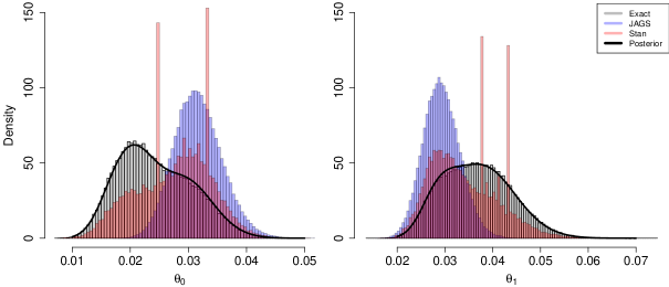
Figure 2: Pathological MCMC posterior sampling exhibited in posterior histograms of the baseline risk $\theta_{0}$ (left) and treatment risk $\theta_{1}$ (right). The marginal posterior of $\theta_{1}$ (black curve) was approximated using numerical integration.

Prior-data conflict, which arises when the prior is concentrated on parameter values that are unlikely given the data, is a common culprit when diagnosing pathological MCMC sampling [112]. This example is no exception. Figure 2 shows histograms of 100,000 posterior samples of $\theta_{0}$ and $\theta_{1}$ drawn using Algorithm 1 (grey), JAGS (blue), and Stan (red). The marginal posterior density is plotted in black for reference. The posterior of $\theta_{0}$ is a mixture of beta distributions and its multimodality is exhibited in the left panel of Figure 2. While Algorithm 1 produces exact posterior samples that fully capture the distribution, JAGS and Stan fail to adequately explore the left-hand mode. Although Stan manages to deviate from the right-hand mode as compared to JAGS, its chains get stuck at $\theta_{0}\approx 0.024$ and $\theta_{0}\approx 0.033$ when the sampler rejects numerous proposal draws. The story is much the same for $\theta_{1}$.

Monotonicity.

Posterior sampling under monotonicity constraints, such as setting $\eta_{s}=0$ or $\eta_{e}=0$, can be obtained with similar procedures, and we thus defer their discussion to the appendix. See Theorems 4-5 of Appendix C.

3.4 Marginal likelihoods and Bayes factors

From a Bayesian perspective, hypothesis testing is essentially a model comparison exercise [70, 71, 98]. Consider two competing hypothesis, $H_{0}$ and $H_{1}$. For each hypothesis $H_{k}$, $k\in\{0,1\}$, the Bayesian approach requires postulating a fully specified model $M_{k}$, with likelihood $L_{k}(\mathcal{D}|\theta)$ and prior $\pi_{k}(\theta)$, respecting the constraints of the hypothesis the model is intended to represent. Evidence in favor of $H_{1}$ relative to $H_{0}$ is then quantified using the Bayes factor $\text{BF}_{10}$, given by the ratio of the marginal likelihoods of the observed data under each model, $\text{BF}_{10}=L_{1}(\mathcal{D})/L_{0}(\mathcal{D})$, where $L_{k}(\mathcal{D})=\int L_{k}(\mathcal{D}|\theta)\pi_{k}(\theta)d\theta$. Given prior model probabilities ${\mathbb{P}(M_{0})}$, ${\mathbb{P}(M_{1})}$, the posterior odds of $M_{1}$ and $M_{0}$ are then ${\mathbb{P}(M_{1}|\mathcal{D})}/{\mathbb{P}(M_{0}|\mathcal{D})}=\text{BF}_{10}\times{\mathbb{P}(M_{1})}/{\mathbb{P}(M_{0})}.$ In this section we show how to formulate such models instantiating a number of relevant statistical hypotheses with the BREASE approach, and provide analytical formulae for the marginal likelihoods. For all models considered here the likelihood is the same, so we focus the discussion on the formulation of the prior.

Let us first consider testing the null hypothesis $H_{0}:\theta_{1}=\theta_{0}$ against the alternative hypothesis $H_{1}:\theta_{1}\neq\theta_{0}$. For $H_{1}$, we propose using the unconstrained model $M_{1}$, with the BREASE prior in (3.5) and equation (3.3),

$$M_{1}:(\theta_{0},\eta_{e},\eta_{s})\sim\text{BREASE}(\mu;n),\qquad\theta_{1}=(1-\eta_{e})\theta_{0}+\eta_{s}(1-\theta_{0}).$$ (3.13)

As for the null hypothesis $H_{0}:\theta_{1}=\theta_{0}$, we instantiate it with the null model,

$$M_{0}:\theta_{0}\sim\text{Beta}^{*}(\mu_{0},n_{0}),\qquad\theta_{1}=\theta_{0}.$$ (3.14)

One benefit of $M_{0}$ is that its prior is logically consistent with the marginal distribution of $\theta_{0}$ under $M_{1}$, both implying $\theta_{0}\sim\text{Beta}^{*}(\mu_{0},n_{0})$ a priori. Note that the prior (3.14) emerges naturally from $M_{1}$ in at least two ways: (i) when postulating that the treatment does not work at all, by setting $\eta_{s}=\eta_{s}=0$; or, (ii) by noting that, if the treatment has no effect on average (i.e, the efficacy of the treatment precisely offsets its side effects), one can side-step thinking about $\eta_{s}$ and $\eta_{e}$ altogether. In both cases, we borrow the prior of $\theta_{0}$ from $M_{1}$, and simply set $\theta_{1}$ equal to $\theta_{0}$. We discuss alternative prior formulations for $H_{0}$ in Appendix E.1.

Other relevant hypothesis one may wish to test are that the treatment is beneficial $H_{-}:\theta_{1}<\theta_{0}$ or that the treatment is harmful $H_{+}:\theta_{1}>\theta_{0}$, on average. A straightforward approach to specify models for such hypotheses is to note that $M_{1}$ already induces positive probabilities to the events postulated in $H_{-}$ and $H_{+}$. Thus, we can borrow this knowledge, already elicited when forming $M_{1}$, to define the priors $\pi_{-}$ and $\pi_{+}$,

$$\pi_{-}(\theta_{0},\eta_{e},\eta_{s}):=\pi_{1}(\theta_{0},\eta_{e},\eta_{s}|\theta_{1}<\theta_{0}),\quad\pi_{+}(\theta_{0},\eta_{e},\eta_{s}):=\pi_{1}(\theta_{0},\eta_{e},\eta_{s}|\theta_{1}>\theta_{0}).$$ (3.15)

The priors $\pi_{-}$ and $\pi_{+}$ result in the models $M_{-}$ and $M_{+}$, for $H_{-}$ and $H_{+}$ respectively. Similarly to $M_{0}$, one benefit of these models is that the induced priors on $(\theta_{0},\eta_{e},\eta_{s})$ are logically consistent with the beliefs expressed in $M_{1}$, under the constraints $H_{-}$ and $H_{+}$. Note that the same strategy employed here can be used for interval hypotheses of the type $H_{0}^{\delta}:|\theta_{1}-\theta_{0}|\leq\delta$, with $\delta>0$ (or, more generally, for any event with nonzero probability under $M_{1}$). Alternative models for $H_{-}$ and $H_{+}$, leveraging instead monotonicity constraints, such as $\eta_{s}=0$ or $\eta_{e}=0$, are discussed in Appendix E.2.

In all cases above, the marginal likelihood can be obtained using analytical formulae and simple Monte Carlo approximation, thereby facilitating the computation of Bayes factors.

Theorem 3.

The marginal likelihood of the data under $M_{0}$ is given by a beta-binomial distribution. Under $M_{1}$, it is given by a weighted sum of beta functions:

$$L_{1}(\mathcal{D}) =\binom{N_{0}}{y_{0}}\binom{N_{1}}{y_{1}}\sum_{j=0}^{y_{1}}\sum_{k=0}^{N_{1}-y_{1}}\binom{y_{1}}{j}\binom{N_{1}-y_{1}}{k}\times\frac{\text{B}(k+\mu_{e}n_{e},j+(1-\mu_{e})n_{e})}{\text{B}(\mu_{e}n_{e},(1-\mu_{e})n_{e})}$$

$$\qquad\times\frac{\text{B}(y_{0}+j+k+\mu_{0}n_{0},N-(y_{0}+j+k)+(1-\mu_{0})n_{0})}{\text{B}(\mu_{0}n_{0},(1-\mu_{0})n_{0})}$$

$$\qquad\times\frac{\text{B}(y_{1}-j+\mu_{s}n_{s},N_{1}-y_{1}-k+(1-\mu_{s})n_{s})}{\text{B}(\mu_{s}n_{s},(1-\mu_{s})n_{s})}.$$ (3.16)

Under $M_{-}$ and $M_{+}$, it can be obtained from $L_{1}(\mathcal{D})$ as follows,

$$L_{-}(\mathcal{D})=L_{1}(\mathcal{D})\times\frac{\pi_{1}(\theta_{1}<\theta_{0}|\mathcal{D})}{\pi_{1}(\theta_{1}<\theta_{0})},\qquad L_{+}(\mathcal{D})=L_{1}(\mathcal{D})\times\frac{\pi_{1}(\theta_{1}>\theta_{0}|\mathcal{D})}{\pi_{1}(\theta_{1}>\theta_{0})}.$$ (3.17)

Proof.

The result for $M_{0}$ is well-known. $L_{1}(\mathcal{D})$ in (3.16) follows directly from integration of (3.4) under the prior (3.5). $L_{-}(\mathcal{D})$ and $L_{+}(\mathcal{D})$ in (3.17) follow from Bayes’ rule. ∎

Remark 1.

The prior and posterior probabilities $\pi_{1}(\theta_{1}<\theta_{0})$ and $\pi_{1}(\theta_{1}<\theta_{0}|\mathcal{D})$ can be approximated using Monte Carlo integration with exact samples, as per Section 3.3.

Remark 2.

As per (3.17), if one postulates prior model probabilities $\mathbb{P}(M_{-}|M_{1})=\pi_{1}(\theta_{1}<\theta_{0})$ and $\mathbb{P}(M_{+}|M_{1})=\pi_{1}(\theta_{1}>\theta_{0})$, the Bayes factor testing $H_{0}:\theta_{1}=\theta_{0}$ against $H_{1}:\theta_{1}\neq\theta_{0}$ (using $M_{1}$) conveniently decomposes into the weighted average of the Bayes factors testing $H_{0}$ against $H_{-}$ (using $M_{-}$) and $H_{0}$ against $H_{+}$ (using $M_{+}$)—though, of course, users can postulate prior probabilities for the models $M_{-}$ and $M_{+}$ as they wish.

As noted by [128], if one reports a Bayes factor comparing models, it is advisable to also report posterior estimates accounting for model uncertainty, i.e., using the implied mixture prior given by the weighted combination of the priors of all models being compared, $\pi(\theta)=\sum_{k}\mathbb{P}(M_{k})\pi_{k}(\theta)$. In this case, samples from the mixture posterior can be readily obtained by sampling from the posterior of each model (as detailed in Section 3.3) proportionally to each model’s posterior probability, $\pi(\theta|\mathcal{D})=\sum_{k}\mathbb{P}(M_{k}|\mathcal{D})\pi_{k}(\theta|\mathcal{D})$.

4 Empirical Examples

We now demonstrate the utility of our approach in three empirical examples. We show how the BREASE framework can be used to facilitate Bayesian estimation, hypothesis testing, and sensitivity analysis of the results of binary experiments. Concretely, the examples illustrate how our proposal can: (i) help analysts distinguish robust from fragile findings; (ii) clarify what one needs to believe in order to claim that a treatment is effective; and (iii) reconcile disparate results obtained from different methods.

4.1 The effect of aspirin on myocardial infarction

We revisit the aspirin component of the Physicians’ Health Study, a large-scale randomized, placebo-controlled trial designed, in part, to investigate whether low-dose aspirin decreases the risk of cardiovascular mortality [92]. During the study, $y_{0}=26$ out of $N_{0}=$ 11,034 subjects in the placebo group experienced fatal myocardial infarction compared to $y_{1}=10$ out of $N_{1}=$ 11,037 prescribed aspirin. Using maximum likelihood estimation, the estimated risk ratio $\theta_{1}/\theta_{0}$ is 0.38, with 95% confidence interval (based on inverting Fisher’s exact test) $\text{CI}(95\%)=[0.17,0.82]$. Consequently, we reject the null hypothesis of zero effect, $H_{0}:\theta_{1}=\theta_{0}$, with $p$-value $0.008$. Results based on asymptotic Wald and Pearson tests are nearly identical. Hence, a frequentist would confidently conclude that low-dose aspirin significantly reduces cardiovascular mortality.

Traditional Bayesian estimation under the alternative hypothesis (i.e, with a prior that gives zero probability to the null hypothesis of zero effect) yields qualitatively similar, though more conservative, answers. Using our default prior, $\text{BREASE}(1/2,.3,.3;2,1,1)$, the posterior median of the risk ratio is 0.44 with a wider 95% credible interval of $\text{CrI}(95\%)=[0.2,0.96]$. The results for the LT and IB approach are similar.

Traditional estimation, however, does not give the null hypothesis of zero effect a fighting chance, as it is assumed to be false a priori. One may thus be interested in performing a Bayesian hypothesis test assigning nonzero prior probability to $H_{0}$. Perhaps surprisingly, a test based on the IB approach yields a Bayes factor $\text{BF}_{01}=20.27$, suggesting that the data provide strong evidence in favor of $H_{0}$. On the other hand, the Bayes factor under the LT approach is $\text{BF}_{10}=5.24$, which suggests moderate evidence in favor of $H_{1}:\theta_{1}\neq\theta_{0}$. Finally, the default BREASE prior results in $\text{BF}_{10}=1.2$ providing essentially little evidence in favor of one hypothesis or the other. How can we make sense of these disparate results? As is well known, Bayes factors are sensitive to the prior distribution [98]. It is important, then, that prior assumptions are encoded in a way that practitioners can understand, both to examine the reasonableness of the prior, as well as to explore how robust inferences are to sensible perturbations of the prior [82, 88, 98].

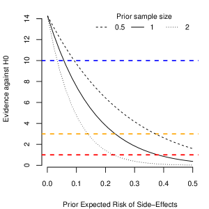
(a) Sensitivity plot varying $\mu_{s}$ and $n_{s}$.

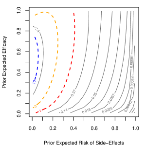
(b) Sensitivity contours varying $\mu_{s}$ and $\mu_{e}$.

Figure 3: Sensitivity analysis of $\text{BF}_{10}$ for the aspirin trial.

One benefit of the BREASE approach is that it allows one to clearly encode prior assumptions in terms of the expected efficacy and side effects of aspirin, and to examine how sensitive the BF is to those assumptions. For example, aspirin is an over-the-counter medicine, with ample usage, and it would thus be unreasonable to expect that aspirin would cause myocardial infarction in a large fraction of otherwise healthy patients. Figure 3(a) inspects how the Bayes factor is affected as we vary the prior expectation of side effects, ranging from 0.01% to 50%, while still keeping relatively vague priors on the baseline risk and efficacy. The dashed red, orange, and blue lines denote (slightly modified) Jeffreys’ thresholds for weak $(1\leq\text{BF}_{10}\leq 3)$, moderate $(3\leq\text{BF}_{10}\leq 10)$, and strong $(\text{BF}_{10}\geq 10)$ evidence against $H_{0}$, respectively [70, 98]. Indeed, as the plot shows, the results are extremely sensitive to the choice of $\mu_{s}$. Setting the expected value of side effects to 1% results in $\text{BF}_{10}=13.45$, yielding strong evidence in favor of $H_{1}$, while setting it to 50% results in $\text{BF}_{01}=2.66$, yielding weak evidence in favor of $H_{0}$. Translating these to posterior probabilities, we have the wide range of 27% to 93% probability of the existence of an effect (assuming equal prior odds for $H_{0}$ and $H_{1}$).

One may also want to conduct a sensitivity analysis with respect to both hyperparameters simultaneously for the $\text{BREASE}(1/2,\mu_{e},\mu_{s};2,1,1)$ prior. Figure 3(b) shows the contour lines of $\text{BF}_{10}$ as a function of $(\mu_{e},\mu_{s})\in(0,1)^{2}$ over their full range of possible values, while keeping $n_{e}=n_{s}=1$ fixed. In general, the results seem more sensitive to plausible variations of the expected risk of side effects $\mu_{s}$ than to plausible variations of the expected efficacy $\mu_{e}$ of aspirin. Overall, only when (i) side effects are expected to be small ($<1\%$), and (ii) the efficacy is expected to be relatively large (between 30% and 70%), does the Bayes factor provide strong evidence against the null of no effect. For all other combinations of prior hyperparameters, the evidence is either moderate, weak, or favors the null. In this light, the results of the trial are ambiguous, and the conclusion that aspirin prevents heart attack strongly depends on the prior. Note that this need not always be the case, as we show next in a reanalysis of the Pfizer-BioNTech COVID-19 vaccine trial.

4.2 The Pfizer-BioNTech COVID-19 vaccine trial

We now reexamine the results of the Pfizer-BioNTech mRNA COVID-19 vaccine study [124]. The experiment was a global multi-phase randomized placebo-controlled trial designed, in part, to evaluate the efficacy of the BNT162b2 vaccine candidate in preventing COVID-19. Vaccine development and evaluation were carried out in rapid response to the emerging SARS-CoV-2 pandemic. The results of the trial were definitive and precipitated the U.S. Food and Drug Administration’s emergency use authorization for widespread dissemination of the vaccine [125].

During the study, $y_{1}=9$ out of $N_{1}=$ 19,965 subjects contracted COVID-19 subsequent to the second dose of the vaccine, while there were $y_{0}=169$ cases out of $N_{0}=$ 20,172 subjects receiving placebo injections. In their paper, [124] adopted a Bayesian approach, focusing particularly on evaluating the vaccine’s efficacy (defined in the study as the estimand $1-\theta_{1}/\theta_{0}$). The efficacy of the vaccine was estimated at 0.95, with credible interval $\text{CrI}(95\%)=[0.90,0.97]$. Frequentist estimates are similar, with a point estimate of 0.95, confidence interval $\text{CI}(95\%)=[0.90,0.97]$, and a $p$-value for testing the null hypothesis of zero effect of the order $6\times 10^{-33}$.

[124] estimate $1-\theta_{1}/\theta_{0}$ as the efficacy of the vaccine, but, as per Section 3.1.2, this only has the counterfactual interpretation of efficacy (i.e., $\eta_{e}=1-\theta_{1}/\theta_{0}$) under the assumption of monotonicity. Using the BREASE approach we can easily encode the monotonicity assumption by setting $\eta_{s}=0$ and then proceed with estimation. The default BREASE prior, with the monotonicity constraint, results in posterior median and 95% credible interval for $\eta_{e}=1-\theta_{1}/\theta_{0}$ that are essentially the same as the previous results, namely, 0.94 and $\text{CrI}(95\%)=[0.90,0.97]$. In the absence of the monotonicity assumption, we have that $1-\theta_{1}/\theta_{0}$ is in fact a lower bound on $\eta_{e}$. Again using the default BREASE prior, results are virtually unchanged, with posterior median and 95% credible interval for $1-\theta_{1}/\theta_{0}$ of 0.94 and $\text{CrI}(95\%)=[0.90,0.97]$. Conclusions using the IB and LT priors are practically equivalent.

(a) Sensitivity plot varying $\mu_{s}$ and $n_{s}$.

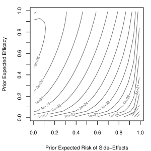
(b) Sensitivity contours varying $\mu_{s}$ and $\mu_{e}$.

Figure 4: Sensitivity analysis of $\text{BF}_{10}$ for the COVID-19 vaccine trial.

Turning to hypothesis testing, differently from the aspirin study, here all approaches point to the same direction, with overwhelming evidence against $H_{0}$. The Bayes factors against the null hypothesis of zero effect are $9\times 10^{33}$, $5\times 10^{34}$ and $4\times 10^{35}$ for the IB, LT and BREASE default priors, respectively. Further, sensitivity analyses reveal the Bayes factor is in fact robust to variations in the hyperparameters across the whole range of prior expected efficacy and side effects of the vaccine, i.e., $(\mu_{e},\mu_{s})\in(0,1)^{2}$. Figure 4 replicates the same sensitivity plots of the aspirin study for the COVID-19 trial. Notice that, in all scenarios, the posterior probability of the null hypothesis is essentially zero even if we posit equal prior odds for $H_{0}$ and $H_{1}$. Therefore, in this case, credible intervals constructed under $H_{1}$, neglecting $H_{0}$, are identical to credible intervals constructed using the mixture prior assigning a point mass of 0.5 to $H_{0}$. The trial provides unequivocal evidence that the vaccine is highly efficacious.

4.3 Null results in the New England Journal of Medicine

[129] conducted a Bayesian reanalysis of 39 binary experiments reporting null results (claiming absence or nonsignificance of an effect of treatment) in the New England Journal of Medicine (NEJM). They were particularly concerned with distinguishing between absence of evidence and evidence of absence of an effect when outcomes in the treatment and control groups are similar. Finding that Bayes factors calculated using the IB approach often strongly favored the null hypothesis (leaning heavily toward evidence of absence) whereas LT Bayes factors were generally equivocal, [129] concluded that the LT approach should be preferred for Bayesian tests for an equality of proportions. In our final empirical example, we expand their reanalysis to include the BREASE approach, and we show how it can easily address the concerns of [129] while also providing a better fit to the data in most cases.

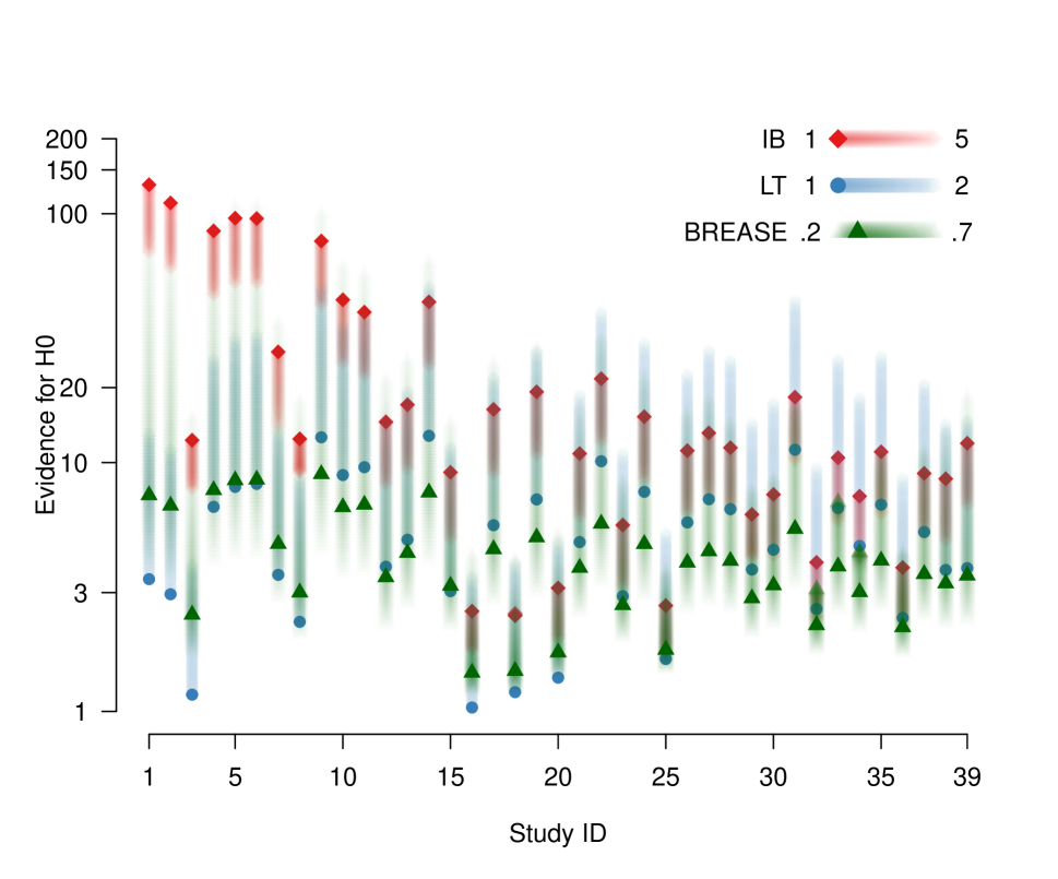
(a) Bayes factors.

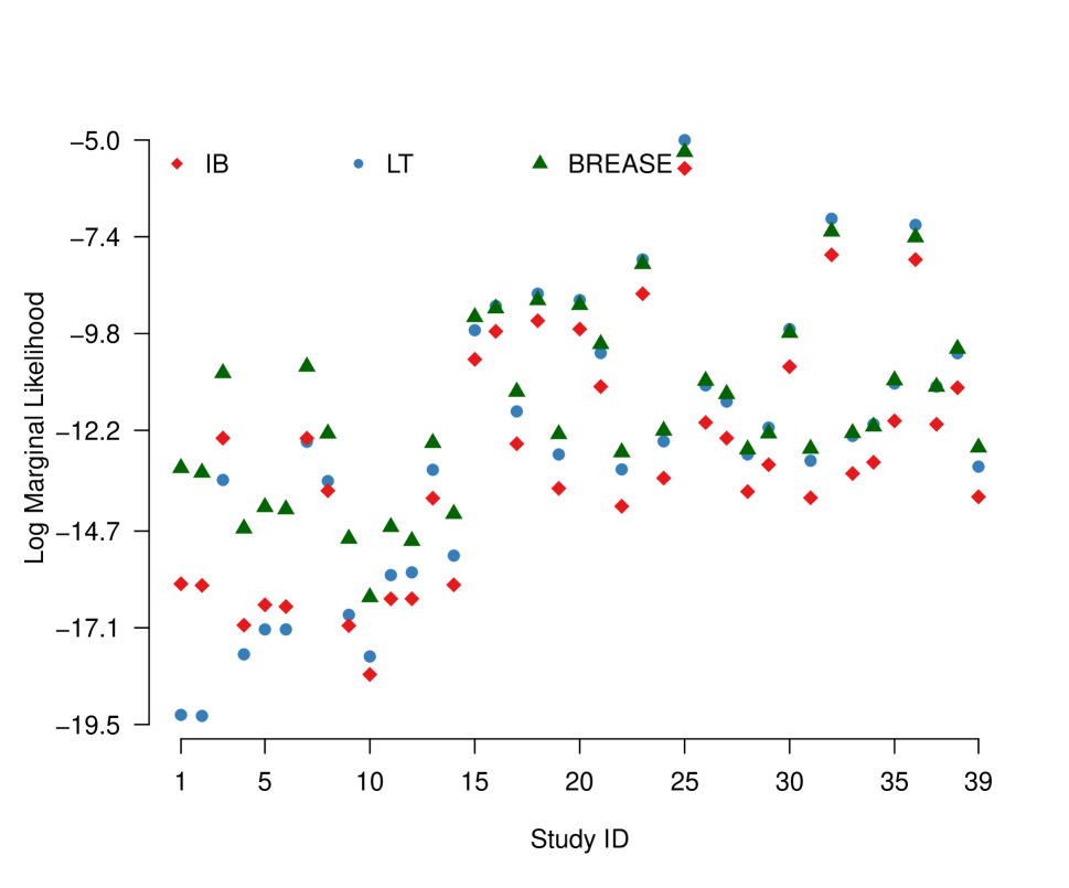
(b) Log marginal likelihoods.

Figure 5: Comparisons of log marginal likelihoods and Bayes factors across 39 NEJM studies, for the IB, LT and BREASE priors.

Figure 5(a) contrasts the Bayes factors in favor of the null hypothesis using: (i) the $\text{IB}(a,a;a,a)$ prior varying $a\in[1,5]$ (red diamonds); (ii) the $\text{LT}(0,0;1,\sigma_{\psi})$ prior varying $\sigma_{\psi}\in[1,2]$ (blue circles); and, the $\text{BREASE}(1/2,\mu,\mu;2,1,1)$ prior varying $\mu\in[.2,.7]$ (green triangles). The solid color stands for the proposed default values of each method, namely $a=1$ for the IB, $\sigma_{\psi}=1$ for the LT and $\mu=.3$ for the BREASE. Note that the Bayes factors of the BREASE and LT default priors (solid triangle and circles) are similar across studies. Moreover, [129] noted that, in many examples, the Bayes factors of the IB and LT approaches could not be easily reconciled, even when reasonably varying their hyperparameters. The BREASE approach shows that this behavior is a mere artifact of those parameterizations. Indeed, for all studies, the BREASE prior easily interpolates between the two regimes, thus solving the apparent contradiction between the results of the LT and IB approaches, by transparently revealing how sensitive inferences are to the prior expected efficacy and side effects of the treatment $\mu$. Finally, Figure 5(b) compares the predictive performance of the default IB, LT, and BREASE priors via the log marginal likelihood. The BREASE prior exhibits superior performance in every study when compared to the IB prior, and in more than 74% of the studies when compared to the LT prior. Thus, in this setting, our proposed default prior seems to provide not only a more sensible parameterization, but also a better fit to the data.

5 Conclusion

We have introduced the BREASE framework for the Bayesian analysis of randomized controlled trials with a binary treatment and outcome. Framing the problem in the language of potential outcomes, we reparameterized the likelihood in terms of clinically meaningful quantities—the baseline risk, efficacy, and risk of adverse side effects of the treatment—and proposed a simple, yet flexible jointly independent beta prior distribution on these parameters. We provided algorithms for exact posterior sampling, as well as analytical formulae for marginal likelihoods, Bayes factors, and other quantities. Finally, we showed with empirical examples how our proposal facilitates estimation, hypothesis testing, elicitation of prior knowledge and sensitivity analysis of treatment effects in binary experiments.

Many interesting extensions of this framework are possible. One possibility is to extend the method to pool evidence across multiple trials. The problem of aggregating evidence is important in its own right, and data from multiple sites may also allow to point identify, or at least narrow the bounds on the fraction of people who benefit or are harmed by the intervention. In a similar vein, another possibility is to extend our framework to the analysis of crossover trials. Under certain assumptions of temporal homogeneity, the efficacy and side effects may be identifiable, making our parameterization and prior proposal natural candidates to the study of treatment effects in such designs.

Acknowledgments.

Irons’s research was supported by a Shanahan Endowment Fellow- ship and a Eunice Kennedy Shriver National Institute of Child Health and Human Development training grant, T32 HD101442-01, to the Center for Studies in Demography & Ecology at the University of Washington.

[sorting=bibsort]

Appendix A Implied prior on $\theta_{1}$

Let the prior of $(\theta_{0},\eta_{e},\eta_{s})$ consist of independent beta distributions with PDFs denoted by $\theta_{0}\sim\pi_{\theta_{0}}(\theta_{0})$, $\eta_{s}\sim\pi_{s}(\eta_{s})$, and $\eta_{e}\sim\pi_{e}(\eta_{e})$. By the law of total probability, the conditional distribution of $\theta_{1}$ given $\theta_{0}$ can be written as

$$\pi(\theta_{1}\mid\theta_{0})=\int_{0}^{1}\pi(\theta_{1}\mid\theta_{0},\eta_{e})\pi_{e}(\eta_{e})d\eta_{e},$$ (A.1)

where here we make use of the fact that $\eta_{e}$ and $\theta_{0}$ are a priori independent. Note that, conditional on $\theta_{0}$ and $\eta_{e}$, $\theta_{1}$ is simply a linear transformation of $\eta_{s}$, namely $\theta_{1}=\theta_{0}(1-\eta_{e})+(1-\theta_{0})\eta_{s}$. We can thus write the density of $\theta_{1}$ in terms of the density of $\eta_{s}$ as

$$\pi(\theta_{1}\mid\theta_{0},\eta_{e})=\left(\frac{1}{1-\theta_{0}}\right)\pi_{s}\left(\frac{\theta_{1}-\theta_{0}(1-\eta_{e})}{1-\theta_{0}}\right),$$

where we make use of the fact that $\displaystyle\frac{d\eta_{s}}{d\theta_{1}}=\frac{1}{1-\theta_{0}}$. Substituting this back into Eq. A.1, we have the following integral

$$\pi(\theta_{1}\mid\theta_{0})=\left(\frac{1}{1-\theta_{0}}\right)\int_{0}^{1}\pi_{s}\left(\frac{\theta_{1}-\theta_{0}(1-\eta_{e})}{1-\theta_{0}}\right)\pi_{e}(\eta_{e})d\eta_{e}.$$ (A.2)

For the special case where $\eta_{e}$ is uniformly distributed, $\pi_{e}(\eta_{e})=1$, the integral simplifies,

$$\pi(\theta_{1}\mid\theta_{0}) =\left(\frac{1}{1-\theta_{0}}\right)\int_{0}^{1}\pi_{s}\left(\frac{\theta_{1}-\theta_{0}(1-\eta_{e})}{1-\theta_{0}}\right)d\eta_{e}$$ (A.3)

$$=\left(\frac{1}{\theta_{0}}\right)\int_{\frac{\theta_{1}-\theta_{0}}{1-\theta_{0}}}^{\frac{\theta_{1}}{1-\theta_{0}}}\pi_{s}\left(\eta_{s}\right)d\eta_{s}$$ (A.4)

$$=\left(\frac{1}{\theta_{0}}\right)\left(F_{s}\left(\frac{\theta_{1}}{1-\theta_{0}}\right)-F_{s}\left(\frac{\theta_{1}-\theta_{0}}{1-\theta_{0}}\right)\right),$$ (A.5)

where the second equality follows from change of variables, noting $d\eta_{e}=(1-\theta_{0})/\theta_{0}d\eta_{s}$. Here $F_{s}(\cdot)$ denotes the CDF of the beta distribution, which is given by the the regularized incomplete beta function.

For special cases the expression above simplifies. For instance, when $\eta_{s}$ is also uniformly distributed, we have that $F_{s}(x)=x$, and we obtain a simple closed form expression for the conditional density. Specifically, for $\theta_{0}\leq 1/2$,

$$\pi(\theta_{1}\mid\theta_{0})=\begin{cases}\dfrac{\theta_{1}}{\theta_{0}(1-\theta_{0})}&\text{if }0\leq\theta_{1}<\theta_{0},\\[10.0pt] \dfrac{1}{1-\theta_{0}}&\text{if }\theta_{0}\leq\theta_{1}<1-\theta_{0},\\[10.0pt] \dfrac{1-\theta_{1}}{\theta_{0}(1-\theta_{0})}&\text{if }1-\theta_{0}\leq\theta_{1}\leq 1,\end{cases}$$ (A.6)

and zero, otherwise. Analogously, for $\theta_{0}\geq 1/2$,

$$\pi(\theta_{1}\mid\theta_{0})=\begin{cases}\dfrac{\theta_{1}}{\theta_{0}(1-\theta_{0})}&\text{if }0\leq\theta_{1}<1-\theta_{0},\\[10.0pt] \dfrac{1}{\theta_{0}}&\text{if }1-\theta_{0}\leq\theta_{1}<\theta_{0},\\[10.0pt] \dfrac{1-\theta_{1}}{\theta_{0}(1-\theta_{0})}&\text{if }\theta_{0}\leq\theta_{1}\leq 1,\end{cases}$$ (A.7)

and zero, otherwise. Notice this is a piece-wise linear function of $\theta_{1}$. Remarkably, however, integrating each region over $\theta_{0}$ results in the following marginal distribution of $\pi(\theta_{1})$,

$$\pi(\theta_{1})=2(-\theta_{1}\log\theta_{1}-(1-\theta_{1})\log(1-\theta_{1})),$$

for $\theta_{1}\in[0,1]$, and zero otherwise, which is twice the entropy of the $\text{Bernoulli}(\theta_{1})$ distribution.

More generally, the distribution of linear combinations of beta random variables was studied in [104] and is given in terms of Appell’s first hypergeometric function $F_{1}$, which is an infinite series in two variables:

$$F_{1}(x,y;a;b_{1},b_{2};c)=\sum_{m_{1}=0}^{\infty}\sum_{m_{2}=0}^{\infty}\frac{\Gamma(a+m_{1}+m_{2})\Gamma(b_{1}+m_{1})\Gamma(b_{2}+m_{2})\Gamma(c)}{\Gamma(a)\Gamma(b_{1})\Gamma(b_{2})\Gamma(c+m_{1}+m_{2})}\frac{x^{m_{1}}}{m_{1}!}\frac{y^{m_{2}}}{m_{2}!}.$$ (A.8)

Appell’s function also has an integral representation given by

$$F_{1}(x,y;a;b_{1},b_{2};c)=\text{B}(a,c-a)^{-1}\int_{0}^{1}u^{a-1}(1-u)^{c-a-1}(1-ux)^{-b_{1}}(1-uy)^{-b_{2}}du.$$ (A.9)

Applying the results of [104] to our setup, the prior on $\theta_{1}$ conditional on $\theta_{0}$ induced by the BREASE prior can be obtained as the following piecewise function: (i) for $\theta_{0}\leq 1/2$, we have

$$\pi(\theta_{1}|\theta_{0}) =I(0\leq\theta_{1}\leq\theta_{0})$$

$$\qquad\times\frac{\theta_{1}^{(1-\mu_{e})n_{e}+\mu_{s}n_{s}-1}(\theta_{0}-\theta_{1})^{\mu_{e}n_{e}-1}\text{B}(\mu_{s}n_{s},(1-\mu_{e})n_{e})}{\theta_{0}^{n_{e}-1}(1-\theta_{0})^{\mu_{s}n_{s}}\text{B}(\mu_{s}n_{s},(1-\mu_{s})n_{s})\text{B}((1-\mu_{e})n_{e},\mu_{e}n_{e})}$$

$$\qquad\times F_{1}\left(\frac{-\theta_{1}}{\theta_{0}-\theta_{1}},\frac{\theta_{1}}{1-\theta_{0}};\mu_{s}n_{s};1-\mu_{e}n_{e},1-(1-\mu_{s})n_{s};(1-\mu_{e})n_{e}+\mu_{s}n_{s}\right)$$

$$+I(\theta_{0}\leq\theta_{1}\leq 1-\theta_{0})$$

$$\qquad\times\frac{(\theta_{1}-\theta_{0})^{\mu_{s}n_{s}-1}(1-\theta_{1})^{(1-\mu_{s})n_{s}-1}}{(1-\theta_{0})^{n_{s}-1}\text{B}(\mu_{s}n_{s},(1-\mu_{s})n_{s})}$$

$$\qquad\times F_{1}\left(\frac{-\theta_{0}}{\theta_{1}-\theta_{0}},\frac{\theta_{0}}{1-\theta_{1}};\mu_{e}n_{e};1-\mu_{s}n_{s},1-(1-\mu_{s})n_{s};n_{e}\right)$$

$$+I(1-\theta_{0}\leq\theta_{1}\leq 1)$$

$$\qquad\times\frac{(1-\theta_{1})^{\mu_{e}n_{e}+(1-\mu_{s})n_{s}-1}(\theta_{1}-\theta_{0})^{\mu_{s}n_{s}-1}\text{B}(\mu_{e}n_{e},(1-\mu_{s})n_{s})}{\theta_{0}^{\mu_{e}n_{e}}(1-\theta_{0})^{n_{s}-1}\text{B}(\mu_{s}n_{s},(1-\mu_{s})n_{s})\text{B}((1-\mu_{e})n_{e},\mu_{e}n_{e})}$$

$$\qquad\times F_{1}\left(\frac{1-\theta_{1}}{\theta_{0}},\frac{\theta_{1}-1}{\theta_{1}-\theta_{0}};\mu_{e}n_{e};1-(1-\mu_{e})n_{e},1-\mu_{s}n_{s};\mu_{e}n_{e}+(1-\mu_{s})n_{s}\right).$$ (A.10)

Similarly, (ii) for $\theta_{0}\geq 1/2$, we have

$$\pi(\theta_{1}|\theta_{0}) =I(0\leq\theta_{1}\leq 1-\theta_{0})$$

$$\qquad\times\frac{\theta_{1}^{(1-\mu_{e})n_{e}+\mu_{s}n_{s}-1}(1-\theta_{0}-\theta_{1})^{(1-\mu_{s})n_{s}-1}\text{B}((1-\mu_{e})n_{e},\mu_{s}n_{s})}{(1-\theta_{0})^{n_{s}-1}\theta_{0}^{(1-\mu_{e})n_{e}}\text{B}((1-\mu_{e})n_{e},\mu_{e}n_{e})\text{B}(\mu_{s}n_{s},(1-\mu_{s})n_{s})}$$

$$\qquad\times F_{1}\left(\frac{-\theta_{1}}{1-\theta_{0}-\theta_{1}},\frac{\theta_{1}}{\theta_{0}};(1-\mu_{e})n_{e};1-(1-\mu_{s})n_{s},1-\mu_{e}n_{e};(1-\mu_{e})n_{e}+\mu_{s}n_{s}\right)$$

$$+I(1-\theta_{0}\leq\theta_{1}\leq\theta_{0})$$

$$\qquad\times\frac{(\theta_{1}-(1-\theta_{0}))^{(1-\mu_{e})n_{e}-1}(1-\theta_{1})^{\mu_{e}n_{e}-1}}{\theta_{0}^{n_{e}-1}\text{B}((1-\mu_{e})n_{e},\mu_{e}n_{e})}$$

$$\qquad\times F_{1}\left(\frac{-(1-\theta_{0})}{\theta_{1}-(1-\theta_{0})},\frac{1-\theta_{0}}{1-\theta_{1}};(1-\mu_{s})n_{s};1-(1-\mu_{e})n_{e},1-\mu_{e}n_{e};n_{s}\right)$$

$$+I(\theta_{0}\leq\theta_{1}\leq 1)$$

$$\qquad\times\frac{(1-\theta_{1})^{\mu_{e}n_{e}+(1-\mu_{s})n_{s}-1}(\theta_{1}-(1-\theta_{0}))^{(1-\mu_{e})n_{e}-1}\text{B}((1-\mu_{s})n_{s},\mu_{e}n_{e})}{(1-\theta_{0})^{(1-\mu_{s})n_{s}}\theta_{0}^{n_{e}-1}\text{B}((1-\mu_{e})n_{e},\mu_{e}n_{e})\text{B}(\mu_{s}n_{s},(1-\mu_{s})n_{s})}$$

$$\qquad\times F_{1}\left(\frac{1-\theta_{1}}{1-\theta_{0}},\frac{\theta_{1}-1}{\theta_{1}-(1-\theta_{0})};(1-\mu_{s})n_{s};1-\mu_{s}n_{s},1-(1-\mu_{e})n_{e};\mu_{e}n_{e}+(1-\mu_{s})n_{s}\right).$$ (A.11)

Monotonicity.

Under the “no harm” monotonicity assumption $\eta_{s}=0$ we have $\theta_{1}=(1-\eta_{e})\theta_{0}$, in which case $\theta_{1}$ is a product of independent beta random variables a priori. [73] derived the form of this distribution, with the density given as a Meijer $G$-function. In general, this function is expressed as a contour integral in the complex plane. However, when $a_{e}=\mu_{e}n_{e}$, $b_{e}=(1-\mu_{e})n_{e}$, $a_{0}=\mu_{0}n_{0}$, and $b_{0}=(1-\mu_{0})n_{0}$ are integers, the prior on $\theta_{1}$ can be expressed in closed form as

$$\pi(\theta_{1})=\frac{\Gamma(n_{0})\Gamma(n_{e})}{\Gamma(\mu_{0}n_{0})\Gamma((1-\mu_{e})n_{e})}\sum_{k=1}^{m}\sum_{j=0}^{e_{k}-1}\frac{K_{kj}\theta_{1}^{d_{k}-1}(-\log\theta_{1})^{e_{k}-j-1}}{\Gamma(e_{k}-j)\Gamma(j+1)},$$

where $\{d_{1},\ldots,d_{m}\}$ denote the $m$ different integers occurring with multiplicity $\{e_{1},\ldots,e_{m}\}$, respectively, among the sets $\{a_{0}-1,\ldots,a_{0}+b_{0}-2\}$ and $\{a_{e}-1,\ldots,a_{e}+b_{e}-2\}$, and

$$K_{kj}=\sum_{r=0}^{j}\sum_{q\in\{1,\ldots,m\},q\neq k}(-1)^{r+1}\binom{j}{r}\frac{\Gamma(r+1)e_{q}}{(d_{q}-d_{k})^{r+1}}.$$

In particular, if $a_{e}+b_{e}=a_{0}$ (equivalently $n_{e}=\mu_{0}n_{0}$, an implicit assumption of the Dirichlet prior), we have

$$\theta_{1}\sim\text{Beta}((1-\mu_{e})n_{e},\mu_{e}n_{e}+(1-\mu_{0})n_{0}).$$

For another example, if $(\theta_{0},\eta_{e})\sim\text{Uniform}(0,1)^{2}$, we have

$$\pi(\theta_{1})=-\log\theta_{1}.$$

Regarding the conditional prior $\pi(\theta_{1}|\theta_{0})$ under the “no harm” assumption, it is clearly a scaled beta distribution, since $\theta_{1}=(1-\eta_{e})\theta_{0}$. If $\eta_{e}\sim\text{Uniform}(0,1)$, we then have that $\theta_{1}|\theta_{0}\sim\text{Uniform}(0,\theta_{0})$. Similarly, under the “no benefit” assumption $\eta_{e}=0$, we have that $\theta_{1}=\theta_{0}+\eta_{s}(1-\theta_{0})$, which is a scaled and shifted beta random variable conditional on $\theta_{0}$. If $\eta_{s}\sim\text{Uniform}(0,1)$, then $\theta_{1}|\theta_{0}\sim\text{Uniform}(\theta_{0},1)$.

As for the moments, applying the law of total covariance to the terms involving $\theta_{1}$ by conditioning on $\theta_{0}$ and making use of equation (3.3), we obtain

$$\text{Cov}(\theta_{0},\theta_{1}) =\frac{\mu_{0}(1-\mu_{0})}{n_{0}+1}(1-\mu_{e}-\mu_{s}),$$

$$\text{Var}(\theta_{0}) =\frac{\mu_{0}(1-\mu_{0})}{n_{0}+1},$$

$$\text{Var}(\theta_{1}) =\frac{\mu_{0}(1-\mu_{0})}{n_{0}+1}(1-\mu_{e}-\mu_{s})^{2}$$

$$\qquad+\frac{\mu_{e}(1-\mu_{e})}{n_{e}+1}\left\{\frac{\mu_{0}(1-\mu_{0})}{n_{0}+1}+\mu_{0}^{2}\right\}$$

$$\qquad+\frac{\mu_{s}(1-\mu_{s})}{n_{s}+1}\left\{\frac{\mu_{0}(1-\mu_{0})}{n_{0}+1}+(1-\mu_{0})^{2}\right\}.$$

This can be used to obtain the prior correlation,

$$\text{Cor}(\theta_{0},\theta_{1}) =\frac{\text{Cov}(\theta_{0},\theta_{1})}{\sqrt{\text{Var}(\theta_{0})\text{Var}(\theta_{1})}}.$$

Figure 6: Heatmaps of the joint density of $(\theta_{0},\theta_{1})$ under the $\text{BREASE}(1/2,\mu,\mu;n,n/2,n/2)$ prior varying $n$ and $\mu$. Our proposed default prior takes $n=2$ and $\mu=.3$. As the plot shows, this: (i) leads to uniform marginals on $\theta_{0}$ and $\theta_{1}$; (ii) assumes zero treatment effect on average; (iii) concentrates mass on the diagonal $\theta_{0}=\theta_{1}$; (iv) favors small (or large) proportions, instead of proportions around the center, which is expected when one quantifies rare outcomes such as death (proportions would be small) or, its complement, survival (in which case proportions would be large).

Appendix B The generalized Dirichlet distribution on $\mathbf{p}$

Given a vector of probabilities $\mathbf{p}=(p_{1},\dots,p_{k})$, such that $\sum_{i=1}^{k}p_{i}=1$, the generalized Dirichlet distribution [108] is defined as,

$$\pi(\mathbf{p})\propto\prod_{i=1}^{k}p_{i}^{a_{i}-1}\prod_{j=1}^{m}\left(\sum_{i=1}^{k}\gamma_{ij}p_{i}\right)^{b_{j}-1}$$ (B.1)

where $\Gamma=(\gamma_{ij})$ is a $k\times m$ known scale matrix. We refer to (B.1) as $\text{GD}(a,b,\Gamma)$. Now consider the vector of potential outcomes $\mathbf{p}=(p_{00},p_{01},p_{10},p_{11})$. By change of variables arguments, if $(\theta_{0},\eta_{e},\eta_{s})\sim\text{BREASE}(\mu;n)$ as in (3.5), it is easy to show that $\mathbf{p}$ has density

$$\pi(\mathbf{p})\propto p_{00}^{(1-\mu_{s})n_{s}-1}p_{01}^{\mu_{s}n_{s}-1}p_{10}^{\mu_{e}n_{e}-1}p_{11}^{(1-\mu_{e})n_{e}-1}(p_{00}+p_{01})^{(1-\mu_{0})n_{0}-n_{s}}(p_{10}+p_{11})^{\mu_{0}n_{0}-n_{e}},$$ (B.2)

which is a $\text{GD}(a,b,\Gamma)$ distribution with parameters

$$a =(\mu_{s}n_{s},(1-\mu_{s})n_{s},\mu_{e}n_{e},(1-\mu_{e})n_{e}),$$

$$b =((1-\mu_{0})n_{0}-n_{s}+1,\mu_{0}n_{0}-n_{e}+1,1,1),$$

$$\Gamma =\begin{bmatrix}1&0&1&0\\ 1&0&0&1\\ 0&1&1&0\\ 0&1&0&1\end{bmatrix}.$$

The prior (B.2) is also a grouped Dirichlet distribution, as defined in [108] and [113] (which is a special case of the generalized Dirichlet). Similarly, the posterior in (3.9) induces the following posterior distribution on the vector $\mathbf{p}$,

$$\pi(\mathbf{p}|\mathcal{D}) \propto p_{00}^{(1-\mu_{s})n_{s}-1}p_{01}^{\mu_{s}n_{s}-1}p_{10}^{\mu_{e}n_{e}-1}p_{11}^{(1-\mu_{e})n_{e}-1}$$

$$\times(p_{00}+p_{01})^{N_{0}-y_{0}+(1-\mu_{0})n_{0}-n_{s}}(p_{10}+p_{11})^{y_{0}+\mu_{0}n_{0}-n_{e}}$$

$$\times(p_{00}+p_{10})^{N_{1}-y_{1}}(p_{01}+p_{11})^{y_{1}},$$

which is again a generalized Dirichlet distribution, $\text{GD}(a,b^{\prime},\Gamma)$, with parameters $a$ and $\Gamma$ as in the prior, and updated parameter $b^{\prime}$ given by

$$b^{\prime} =(N_{0}+y_{0}+(1-\mu_{0})n_{0}-n_{s}+1,y_{0}+\mu_{0}n_{0}-n_{e}+1,N_{1}-y_{1}+1,y_{1}+1).$$

The generalized Dirichlet distribution of [87], as well as special cases, such as the grouped Dirichlet and Dirichlet-beta, have been proposed for the Bayesian analysis of categorical data and contingency tables with missing observations [72, 74, 77, 88, 91, 108, 113]. These studies largely focused on the derivation of closed-form expressions (when available) and accurate approximations for posterior moments and predictive probabilities used in estimation and inference. They did not address the parameterization and interpretation of the generalized Dirichlet in terms of the baseline risk, efficacy, and side effects; algorithms for exact posterior simulation; testing for an effect of treatment and sensitivity analysis using analytical formulae; or the specific application to and prior elicitation for binary experiments.

The Dirichlet as a product of independent betas.

To better understand the connection of the BREASE prior with the traditional Dirichlet distribution, it is instructive to first derive the distribution of $(\theta_{0},\eta_{e},\eta_{s})$ induced by a Dirichlet prior on the response type probabilities $\mathbf{p}$. The BREASE parameters can be expressed as

$$\theta_{0}=p_{10}+p_{11},\qquad\eta_{e}=\frac{p_{10}}{p_{10}+p_{11}},\qquad\eta_{s}=\frac{p_{01}}{p_{00}+p_{01}}.$$

Elementary properties of the Dirichlet distribution then imply that these quantities are mutually independent beta random variables [117]

$$\theta_{0}\sim\text{Beta}(a_{10}+a_{11},a_{00}+a_{01})\quad\perp\!\!\!\perp\quad\eta_{e}\sim\text{Beta}(a_{10},a_{11})\quad\perp\!\!\!\perp\quad\eta_{s}\sim\text{Beta}(a_{01},a_{00}).$$ (B.3)

Similarly, since $\theta_{1}=p_{01}+p_{11}$, we also have that $\theta_{1}\sim\text{Beta}(a_{01}+a_{11},a_{00}+a_{10})$ marginally.

While the Dirichlet density seems like a natural choice for the probability vector $\mathbf{p}$, the implied distribution on $(\theta_{0},\eta_{e},\eta_{s})$ reveals some implicit assumptions. In particular, this prior has the peculiar (and potentially undesirable) feature that once we have decided on the parameters underlying the marginal distribution of the efficacy and side effects of treatment $(\eta_{e},\eta_{s})$—which requires specifying $(a_{00},a_{10},a_{01},a_{11})$—we have fully determined the joint prior on $(\theta_{0},\eta_{e},\eta_{s})$. In this sense, the Dirichlet distribution is underparametrized.

This underparameterization becomes clearer with an alternative representation of the beta distribution, in terms of the prior mean and prior “sample size.” For $\mu=a/(a+b)$ and $n=a+b$, we write $\text{Beta}^{*}(\mu,n)$ to denote a $\text{Beta}(a,b)$ distribution, with mean $\mu$ and sample size $n$. The Dirichlet joint prior on $(\theta_{0},\eta_{e},\eta_{s})$ has then the following alternative stochastic representation,

$$\theta_{0}\sim\text{Beta}^{*}(\mu_{0},n_{0})\quad\perp\!\!\!\perp\quad\eta_{e}\sim\text{Beta}^{*}(\mu_{e},\mu_{0}n_{0})\quad\perp\!\!\!\perp\quad\eta_{s}\sim\text{Beta}^{*}(\mu_{s},(1-\mu_{0})n_{0}),$$ (B.4)

which is equivalent to the BREASE prior imposing a restriction on the choice of prior sample sizes $n_{e}$ and $n_{s}$. Marginally, we also have

$$\theta_{1}\sim\text{Beta}^{*}\left((1-\mu_{e})\mu_{0}+\mu_{s}(1-\mu_{0}),n_{0}\right),$$ (B.5)

which mirrors the decomposition (3.3).

Appendix C Posterior sampling

C.1 Proof of Theorem 2

We now describe in greater detail how to sample exactly from the BREASE posterior distribution via simulation.

Proof of Theorem 2.

Let $I_{0}=\{1,\ldots,N_{0}\},I_{1}=\{N_{0}+1,\ldots,N_{0}+N_{1}\}$ denote the indices of subjects in the control and treatment groups, respectively. Define the counterfactual counts

$$y_{j}(k) =\sum_{i\in I_{j}}I(Y_{i}(j)=1,Y_{i}(1-j)=k),$$

$$x_{j}(k) =\sum_{i\in I_{j}}I(Y_{i}(j)=0,Y_{i}(1-j)=k),\qquad j,k\in\{0,1\}.$$

For example, $y_{1}(0)$ is the number of subjects in the treatment group who died but would not have if untreated. Similarly, $x_{1}(1)$ is the number of subjects in the treatment group who did not die but would have if untreated. The posterior can then be expressed as a mixture distribution:

$$\pi(\theta_{0},\eta_{e},\eta_{s}|\mathcal{D})=$$

$$\qquad\qquad\sum_{y_{1}(0)=0}^{y_{1}}\sum_{x_{1}(1)=0}^{N_{1}-y_{1}}\pi(\theta_{0},\eta_{e},\eta_{s}|y_{1}(0),x_{1}(1),\mathcal{D})\times\pi(y_{1}(0),x_{1}(1)|\mathcal{D}).$$ (C.1)

We will derive each term in the sum. A straightforward calculation shows that

$$(y_{0}(0),y_{0}(1),x_{0}(0),x_{0}(1)) |(\theta_{0},\eta_{e},\eta_{s},N_{0})\sim$$

$$\text{Multinomial}_{N_{0}}(\theta_{0}\eta_{e},\theta_{0}(1-\eta_{e}),(1-\theta_{0})(1-\eta_{s}),(1-\theta_{0})\eta_{s}),$$

$$(y_{1}(0),y_{1}(1),x_{1}(0),x_{1}(1)) |(\theta_{0},\eta_{e},\eta_{s},N_{1})\sim$$

$$\text{Multinomial}_{N_{1}}((1-\theta_{0})\eta_{s},\theta_{0}(1-\eta_{e}),(1-\theta_{0})(1-\eta_{s}),\theta_{0}\eta_{e}),$$

and the two distributions are independent. Since

$$y_{1}=y_{1}(0)+y_{1}(1)\qquad\text{and}\qquad N_{1}-y_{1}=x_{1}(0)+x_{1}(1),$$

it follows that

$$y_{1}(0)|(y_{1},\theta_{0},\eta_{e},\eta_{s}) \sim\text{Binomial}\left(y_{1},\frac{(1-\theta_{0})\eta_{s}}{\theta_{1}}\right),$$

$$x_{1}(1)|(y_{1},N_{1},\theta_{0},\eta_{e},\eta_{s}) \sim\text{Binomial}\left(N_{1}-y_{1},\frac{\theta_{0}\eta_{e}}{1-\theta_{1}}\right),$$

independently. Consequently, we have

$$\pi (\theta_{0},\eta_{e},\eta_{s}|y_{1}(0),x_{1}(1),\mathcal{D})$$

$$\propto\pi(y_{1}(0),x_{1}(1),\mathcal{D}|\theta_{0},\eta_{e},\eta_{s})\times\pi(\theta_{0},\eta_{e},\eta_{s})$$

$$=\pi(y_{1}(0),x_{1}(1)|\mathcal{D},\theta_{0},\eta_{e},\eta_{s})\times\pi(\mathcal{D}|\theta_{0},\eta_{e},\eta_{s})\times\pi(\theta_{0},\eta_{e},\eta_{s})$$

$$=\pi(y_{1}(0)|y_{1},\theta_{0},\eta_{e},\eta_{s})\times\pi(x_{1}(1)|y_{1},N_{1},\theta_{0},\eta_{e},\eta_{s})$$

$$\qquad\times\pi(\mathcal{D}|\theta_{0},\eta_{e},\eta_{s})\times\pi(\theta_{0},\eta_{e},\eta_{s})$$

$$=\text{Binomial}\left(y_{1}(0);y_{1},\frac{(1-\theta_{0})\eta_{s}}{\theta_{1}}\right)\times\text{Binomial}\left(x_{1}(1);N_{1}-y_{1},\frac{\theta_{0}\eta_{e}}{1-\theta_{1}}\right)$$

$$\qquad\times\text{Binomial}(y_{0};N_{0},\theta_{0})\times\text{Binomial}(y_{1};N_{1},\theta_{1})$$

$$\qquad\times\text{Beta}(\theta_{0};\mu_{0}n_{0},(1-\mu_{0})n_{0})\times\text{Beta}(\eta_{e};\mu_{e}n_{e},(1-\mu_{e})n_{e})\times\text{Beta}(\eta_{s};\mu_{s}n_{s},(1-\mu_{s})n_{s})$$

$$\propto\theta_{0}^{y_{0}+y_{1}-y_{1}(0)+x_{1}(1)+\mu_{0}n_{0}-1}(1-\theta_{0})^{N-(y_{0}+y_{1}-y_{1}(0)+x_{1}(1))+(1-\mu_{0})n_{0}-1}$$

$$\qquad\times\eta_{e}^{x_{1}(1)+\mu_{e}n_{e}-1}(1-\eta_{e})^{y_{1}-y_{1}(0)+(1-\mu_{e})n_{e}-1}$$

$$\qquad\times\eta_{s}^{y_{1}(0)+\mu_{s}n_{s}-1}(1-\eta_{s})^{N_{1}-y_{1}-x_{1}(1)+(1-\mu_{s})n_{s}-1}.$$

It follows that

$$\pi (\theta_{0},\eta_{e},\eta_{s}|y_{1}(0),x_{1}(1),\mathcal{D})$$

$$=\text{Beta}(\theta_{0};y_{0}+y_{1}-y_{1}(0)+x_{1}(1)+\mu_{0}n_{0},N-(y_{0}+y_{1}-y_{1}(0)+x_{1}(1))+(1-\mu_{0})n_{0})$$

$$\qquad\times\text{Beta}(\eta_{e};x_{1}(1)+\mu_{e}n_{e},y_{1}-y_{1}(0)+(1-\mu_{e})n_{e})$$

$$\qquad\times\text{Beta}(\eta_{s};y_{1}(0)+\mu_{s}n_{s},N_{1}-y_{1}-x_{1}(1)+(1-\mu_{s})n_{s}).$$ (C.2)

Similarly, for the mixture weights we have

$$\pi (y_{1}(0),x_{1}(1)|\mathcal{D})=\int\pi(y_{1}(0),x_{1}(1),\theta_{0},\eta_{e},\eta_{s}|\mathcal{D})d\theta_{0}d\eta_{e}d\eta_{s}$$

$$=\int\pi(y_{1}(0),x_{1}(1)|\theta_{0},\eta_{e},\eta_{s},\mathcal{D})\pi(\theta_{0},\eta_{e},\eta_{s}|\mathcal{D})d\theta_{0}d\eta_{e}d\eta_{s}$$

$$\propto\binom{y_{1}}{y_{1}(0)}\binom{N_{1}-y_{1}}{x_{1}(1)}\text{B}(x_{1}(1)+\mu_{e}n_{e},y_{1}-y_{1}(0)+(1-\mu_{e})n_{e})$$

$$\qquad\times\text{B}(y_{0}+y_{1}-y_{1}(0)+x_{1}(1)+\mu_{0}n_{0},N-(y_{0}+y_{1}-y_{1}(0)+x_{1}(1))+(1-\mu_{0})n_{0})$$

$$\qquad\times\text{B}(y_{1}(0)+\mu_{s}n_{s},N_{1}-y_{1}-x_{1}(1)+(1-\mu_{s})n_{s}).$$ (C.3)

Hence, we can sample from the mixture distribution (3.10) as follows:

1. Sample the unobserved count $x_{1}(1)\in\{0,\ldots,N_{1}-y_{1}\}$ conditional on $\mathcal{D}$ with probability

   $$\pi(x_{1}(1)|\mathcal{D})=\sum_{y_{1}(0)=0}^{y_{1}}\pi(y_{1}(0),x_{1}(1)|\mathcal{D}).$$

   according to (3.11)

2. Sample $y_{1}(0)\in\{0,\ldots,y_{1}\}$ conditional on $(x_{1}(1),\mathcal{D})$ with probability

   $$\pi(y_{1}(0)|x_{1}(1),\mathcal{D})\propto\pi(y_{1}(0),x_{1}(1)|\mathcal{D}).$$

   according to (3.11),

3. Sample $(\theta_{0},\eta_{e},\eta_{s})$ conditional on $(y_{1}(0),x_{1}(1),\mathcal{D})$ from the independent beta distribution (3.12).

∎

C.2 Sampling under monotonicity: no harm

Here we derive the BREASE posterior sampling algorithm under the “no harm” $(\eta_{s}=0)$ monotonicity model $M_{-}^{{}^{\prime}}$ (E.1).

Theorem 4.

Let $(\theta_{0},\eta_{e})$ be random variables drawn according to Algorithm 2. Then $(\theta_{0},\eta_{e})$ are distributed according to the posterior of model $M_{-}^{{}^{\prime}}$ (E.1).

Proof.

In this case, we make use of the posterior mixture representation

$$\pi(\theta_{0},\eta_{e}|\mathcal{D})=\sum_{x_{1}(1)=0}^{N_{1}-y_{1}}\pi(\theta_{0},\eta_{e}|x_{1}(1),\mathcal{D})\times\pi(x_{1}(1)|\mathcal{D}).$$ (C.4)

As discussed in Section C.1, we have

$$x_{1}(1)|(y_{1},N_{1},\theta_{0},\eta_{e})\sim\text{Binomial}\left(N_{1}-y_{1},\frac{\theta_{0}\eta_{e}}{1-\theta_{1}}\right).$$

Note that $\theta_{1}=(1-\eta_{e})\theta_{0}$ by hypothesis. Consequently, we have

$$\pi (\theta_{0},\eta_{e}|x_{1}(1),\mathcal{D})$$

$$\propto\pi(x_{1}(1),\mathcal{D}|\theta_{0},\eta_{e})\times\pi(\theta_{0},\eta_{e})$$

$$=\pi(x_{1}(1)|\mathcal{D},\theta_{0},\eta_{e})\times\pi(\mathcal{D}|\theta_{0},\eta_{e})\times\pi(\theta_{0},\eta_{e})$$

$$=\pi(x_{1}(1)|y_{1},N_{1},\theta_{0},\eta_{e})\times\pi(\mathcal{D}|\theta_{0},\eta_{e})\times\pi(\theta_{0},\eta_{e})$$

$$=\text{Binomial}\left(x_{1}(1);N_{1}-y_{1},\frac{\theta_{0}\eta_{e}}{1-\theta_{1}}\right)\times\text{Binomial}(y_{0};N_{0},\theta_{0})\times\text{Binomial}(y_{1};N_{1},\theta_{1})$$

$$\qquad\times\text{Beta}(\theta_{0};\mu_{0}n_{0},(1-\mu_{0})n_{0})\times\text{Beta}(\eta_{e};\mu_{e}n_{e},(1-\mu_{e})n_{e})$$

$$\propto\theta_{0}^{y_{0}+y_{1}+x_{1}(1)+\mu_{0}n_{0}-1}(1-\theta_{0})^{N-(y_{0}+y_{1}+x_{1}(1))+(1-\mu_{0})n_{0}-1}$$

$$\qquad\times\eta_{e}^{x_{1}(1)+\mu_{e}n_{e}-1}(1-\eta_{e})^{y_{1}+(1-\mu_{e})n_{e}-1}.$$

It follows that

$$\pi(\theta_{0},\eta_{e}| x_{1}(1),\mathcal{D})$$

$$=\text{Beta}(\theta_{0};y_{0}+y_{1}+x_{1}(1)+\mu_{0}n_{0},N-(y_{0}+y_{1}+x_{1}(1))+(1-\mu_{0})n_{0})$$

$$\qquad\times\text{Beta}(\eta_{e};x_{1}(1)+\mu_{e}n_{e},y_{1}+(1-\mu_{e})n_{e}).$$ (C.5)

Similarly, for the mixture weights we have

$$\pi(x_{1}(1)| \mathcal{D})=\int\pi(x_{1}(1),\theta_{0},\eta_{e}|\mathcal{D})d\theta_{0}d\eta_{e}$$

$$=\int\pi(x_{1}(1)|\theta_{0},\eta_{e},\mathcal{D})\pi(\theta_{0},\eta_{e}|\mathcal{D})d\theta_{0}d\eta_{e}$$

$$\propto\binom{N_{1}-y_{1}}{x_{1}(1)}\text{B}(x_{1}(1)+\mu_{e}n_{e},y_{1}+(1-\mu_{e})n_{e})$$

$$\qquad\times\text{B}(y_{0}+y_{1}+x_{1}(1)+\mu_{0}n_{0},N-(y_{0}+y_{1}+x_{1}(1))+(1-\mu_{0})n_{0}).$$ (C.6)

Algorithm 2 defines the procedure to sample from the distribution C.4 based on these calculations. ∎

Algorithm 2 “No harm” $(\eta_{s}=0)$ posterior sampling algorithm

Input: Data $\mathcal{D}=(y_{0},y_{1},N_{0},N_{1})$, hyperparameters $(\mu_{0},\mu_{e},n_{0},n_{e})$, and desired number of posterior samples $T$.

Iterate: For sample $t\in\{1,\ldots,T\}$,

1. Sample $x_{1}(1)\in\{0,\ldots,N_{1}-y_{1}\}$ conditional on $\mathcal{D}$ with probability $\pi(x_{1}(1)|\mathcal{D})$ given by (C.6).

2. Sample $(\theta_{0},\eta_{e})$ conditional on $(x_{1}(1),\mathcal{D})$ from the independent beta distribution (C.5).

Output: Posterior samples $\{(\theta_{0}^{(t)},\eta_{e}^{(t)})\}_{t\in\{1,\ldots,T\}}$.

C.3 Sampling under monotonicity: no benefit

Here we derive the BREASE posterior sampling algorithm under the “no benefit” $(\eta_{e}=0)$ monotonicity model $M_{+}^{{}^{\prime}}$ (E.2).

Theorem 5.

Let $(\theta_{0},\eta_{s})$ be random variables drawn according to Algorithm 3. Then $(\theta_{0},\eta_{s})$ are distributed according to the posterior of model $M_{+}^{{}^{\prime}}$ (E.2).

Proof.

In this case, we make use of the posterior mixture representation

$$\pi(\theta_{0},\eta_{s}|\mathcal{D})=\sum_{y_{1}(0)=0}^{y_{1}}\pi(\theta_{0},\eta_{s}|y_{1}(0),\mathcal{D})\times\pi(y_{1}(0)|\mathcal{D}).$$ (C.7)

As discussed in Section C.1, we have

$$y_{1}(0)|(y_{1},\theta_{0},\eta_{s})\sim\text{Binomial}\left(y_{1},\frac{(1-\theta_{0})\eta_{s}}{\theta_{1}}\right).$$

Note that $\theta_{1}=\theta_{0}+(1-\theta_{0})\eta_{s}$ by hypothesis. Consequently, we have

$$\pi(\theta_{0},\eta_{s}| y_{1}(0),\mathcal{D})$$

$$\propto\pi(y_{1}(0),\mathcal{D}|\theta_{0},\eta_{s})\times\pi(\theta_{0},\eta_{s})$$

$$=\pi(y_{1}(0)|\mathcal{D},\theta_{0},\eta_{s})\times\pi(\mathcal{D}|\theta_{0},\eta_{s})\times\pi(\theta_{0},\eta_{s})$$

$$=\pi(y_{1}(0)|y_{1},\theta_{0},\eta_{s})\times\pi(\mathcal{D}|\theta_{0},\eta_{s})\times\pi(\theta_{0},\eta_{s})$$

$$=\text{Binomial}\left(y_{1}(0);y_{1},\frac{(1-\theta_{0})\eta_{s}}{\theta_{1}}\right)\times\text{Binomial}(y_{0};N_{0},\theta_{0})\times\text{Binomial}(y_{1};N_{1},\theta_{1})$$

$$\qquad\times\text{Beta}(\theta_{0};\mu_{0}n_{0},(1-\mu_{0})n_{0})\times\text{Beta}(\eta_{s};\mu_{s}n_{s},(1-\mu_{s})n_{s})$$

$$\propto\theta_{0}^{y_{0}+y_{1}-y_{1}(0)+\mu_{0}n_{0}-1}(1-\theta_{0})^{N-(y_{0}+y_{1}-y_{1}(0))+(1-\mu_{0})n_{0}-1}$$

$$\qquad\times\eta_{s}^{y_{1}(0)+\mu_{s}n_{s}-1}(1-\eta_{s})^{N_{1}-y_{1}+(1-\mu_{s})n_{s}-1}.$$

It follows that

$$\pi(\theta_{0},\eta_{s}| y_{1}(0),\mathcal{D})$$

$$=\text{Beta}(\theta_{0};y_{0}+y_{1}-y_{1}(0)+\mu_{0}n_{0},N-(y_{0}+y_{1}-y_{1}(0))+(1-\mu_{0})n_{0})$$

$$\qquad\times\text{Beta}(\eta_{s};y_{1}(0)+\mu_{s}n_{s},N_{1}-y_{1}+(1-\mu_{s})n_{s}).$$ (C.8)

Similarly, for the mixture weights we have

$$\pi(y_{1}(0)| \mathcal{D})=\int\pi(y_{1}(0),\theta_{0},\eta_{s}|\mathcal{D})d\theta_{0}d\eta_{s}$$

$$=\int\pi(y_{1}(0)|\theta_{0},\eta_{s},\mathcal{D})\pi(\theta_{0},\eta_{s}|\mathcal{D})d\theta_{0}d\eta_{s}$$

$$\propto\binom{y_{1}}{y_{1}(0)}\text{B}(y_{0}+y_{1}-y_{1}(0)+\mu_{0}n_{0},N-(y_{0}+y_{1}-y_{1}(0))+(1-\mu_{0})n_{0})$$

$$\qquad\times\text{B}(y_{1}(0)+\mu_{s}n_{s},N_{1}-y_{1}+(1-\mu_{s})n_{s}).$$ (C.9)

Algorithm 3 defines the procedure to sample from the distribution C.7 based on these calculations. ∎

Algorithm 3 “No benefit” $(\eta_{e}=0)$ posterior sampling algorithm

Input: Data $\mathcal{D}=(y_{0},y_{1},N_{0},N_{1})$, hyperparameters $(\mu_{0},\mu_{s},n_{0},n_{s})$, and desired number of posterior samples $T$.

Iterate: For sample $t\in\{1,\ldots,T\}$,

1. Sample $y_{1}(0)\in\{0,\ldots,y_{1}\}$ conditional on $\mathcal{D}$ with probability $\pi(y_{1}(0)|\mathcal{D})$ given by (C.9).

2. Sample $(\theta_{0},\eta_{s})$ conditional on $(y_{1}(0),\mathcal{D})$ from the independent beta distribution (C.8).

Output: Posterior samples $\{(\theta_{0}^{(t)},\eta_{s}^{(t)})\}_{t\in\{1,\ldots,T\}}$.

C.4 Sampling with an alternate prior under $H_{0}:\theta_{0}=\theta_{1}$

We now derive a sampling algorithm for the aggregated Dirichlet prior under $H_{0}$ introduced in Section E.1.1:

$$\mathbf{p}^{*}=(p_{00},p^{*}_{10},p_{11})\sim\text{Dirichlet}((1-\mu_{s})n_{s},\mu_{e}n_{e}+\mu_{s}n_{s},(1-\mu_{e})n_{e}),\qquad p^{*}_{10}=p_{10}+p_{01}.$$

The algorithm is based on the posterior decomposition

$$\pi(\mathbf{p}^{*}|\mathcal{D})=\sum_{w(0)=0}^{y_{0}+y_{1}}\sum_{w(1)=0}^{N_{0}+N_{1}-y_{0}-y_{1}} \pi(\mathbf{p}^{*}|w(0),w(1),\mathcal{D})\times\pi(w(0),w(1)|\mathcal{D}),$$ (C.10)

where

$$w(0)=y_{0}(0)+y_{1}(0),\qquad w(1)=x_{0}(1)+x_{1}(1).$$

We have

$$(y_{0}(0),y_{0}(1),x_{0}(0),x_{0}(1)) |(\mathbf{p}^{*},N_{0})\sim\text{Multinomial}_{N_{0}}(p^{*}_{10}/2,p_{11},p_{00},p^{*}_{10}/2),$$

$$(y_{1}(0),y_{1}(1),x_{1}(0),x_{1}(1)) |(\mathbf{p}^{*},N_{1})\sim\text{Multinomial}_{N_{1}}(p^{*}_{10}/2,p_{11},p_{00},p^{*}_{10}/2),$$

and the two distributions are independent. It follows that

$$y_{0}(0)|(y_{0},\mathbf{p}^{*}) \sim\text{Binomial}\left(y_{0},\frac{p^{*}_{10}}{p^{*}_{10}+2p_{11}}\right),$$

$$x_{0}(1)|(y_{0},N_{0},\mathbf{p}^{*}) \sim\text{Binomial}\left(N_{0}-y_{0},\frac{p^{*}_{10}}{p^{*}_{10}+2p_{00}}\right),$$

$$y_{1}(0)|(y_{1},\mathbf{p}^{*}) \sim\text{Binomial}\left(y_{1},\frac{p^{*}_{10}}{p^{*}_{10}+2p_{11}}\right),$$

$$x_{1}(1)|(y_{1},N_{1},\mathbf{p}^{*}) \sim\text{Binomial}\left(N_{1}-y_{1},\frac{p^{*}_{10}}{p^{*}_{10}+2p_{00}}\right),$$

independently. Hence, $w(0)$ and $w(1)$ are distributed independently as

$$w(0)|(y_{0},y_{1},\mathbf{p}^{*}) \sim\text{Binomial}\left(y_{0}+y_{1},\frac{p^{*}_{10}}{p^{*}_{10}+2p_{11}}\right),$$

$$w(1)|(\mathcal{D},\mathbf{p}^{*}) \sim\text{Binomial}\left(N_{0}+N_{1}-y_{0}-y_{1},\frac{p^{*}_{10}}{p^{*}_{10}+2p_{00}}\right),$$

Consequently, we have

$$\pi(\mathbf{p}^{*}|w(0), w(1),\mathcal{D})$$

$$\propto\pi(w(0),w(1),\mathcal{D}|\mathbf{p}^{*})\times\pi(\mathbf{p}^{*})$$

$$=\pi(w(0),w(1)|\mathcal{D},\mathbf{p}^{*})\times\pi(\mathcal{D}|\mathbf{p}^{*})\times\pi(\mathbf{p}^{*})$$

$$=\pi(w(0)|y_{0},y_{1},\mathbf{p}^{*})\times\pi(w(1)|\mathcal{D},\mathbf{p}^{*})$$

$$\qquad\times\pi(\mathcal{D}|\mathbf{p}^{*})\times\pi(\mathbf{p}^{*})$$

$$=\text{Binomial}\left(w(0);y_{0}+y_{1},\frac{p^{*}_{10}}{p^{*}_{10}+2p_{11}}\right)$$

$$\qquad\times\text{Binomial}\left(w(1);N_{0}+N_{1}-y_{0}-y_{1},\frac{p^{*}_{10}}{p^{*}_{10}+2p_{00}}\right)$$

$$\qquad\times\text{Binomial}(y_{0};N_{0},p^{*}_{10}/2+p_{11})\times\text{Binomial}(y_{1};N_{1},p^{*}_{10}/2+p_{11})$$

$$\qquad\times(p^{*}_{10})^{\mu_{e}n_{e}+\mu_{s}n_{s}-1}p_{11}^{(1-\mu_{e})n_{e}-1}p_{00}^{(1-\mu_{s})n_{s}-1}$$

$$\propto(p^{*}_{10})^{w(0)+w(1)+\mu_{e}n_{e}+\mu_{s}n_{s}-1}p_{11}^{y_{0}+y_{1}-w(0)+(1-\mu_{e})n_{e}-1}p_{00}^{N_{0}+N_{1}-y_{0}-y_{1}-w(1)+(1-\mu_{s})n_{s}-1}$$

It follows that

$$\mathbf{p}^{*}|(w(0),w(1),\mathcal{D}) \sim\text{Dirichlet}(a_{00},a_{10},a_{11}),$$ (C.11)

where

$$a_{00} =N_{0}+N_{1}-y_{0}-y_{1}-w(1)+(1-\mu_{s})n_{s},$$

$$a_{10} =w(0)+w(1)+\mu_{e}n_{e}+\mu_{s}n_{s},$$

$$a_{11} =y_{0}+y_{1}-w(0)+(1-\mu_{e})n_{e}.$$

Consequently, for the mixture weights we have

$$\pi (w(0),w(1)|\mathcal{D})=\int\pi(w(0),w(1),\mathbf{p}^{*}|\mathcal{D})d\mathbf{p}^{*}$$

$$=\int\pi(w(0),w(1)|\mathbf{p}^{*},\mathcal{D})\pi(\mathbf{p}^{*}|\mathcal{D})d\mathbf{p}^{*}$$

$$\propto\binom{y_{0}+y_{1}}{w(0)}\binom{N_{0}+N_{1}-y_{0}-y_{1}}{w(1)}$$

$$\qquad\times\int(p^{*}_{10}/2)^{w(0)+w(1)+\mu_{e}n_{e}+\mu_{s}n_{s}-1}p_{11}^{y_{0}+y_{1}-w(0)+(1-\mu_{e})n_{e}-1}p_{00}^{N_{0}+N_{1}-y_{0}-y_{1}-w(1)+(1-\mu_{s})n_{s}-1}d\mathbf{p}^{*}$$

$$\propto 2^{-(w(0)+w(1))}\binom{y_{0}+y_{1}}{w(0)}\binom{N_{0}+N_{1}-y_{0}-y_{1}}{w(1)}\text{B}(a_{00},a_{10},a_{11}).$$ (C.12)

Algorithm 4 defines the procedure to sample from the distribution C.10 based on these calculations.

Algorithm 4 Alternate $H_{0}:\theta_{0}=\theta_{1}$ posterior sampling algorithm

Input: Data $(y_{0},y_{1},N_{0},N_{1})$, hyperparameters $(\mu_{e},\mu_{s},n_{e},n_{s})$, and posterior samples $T$.

Iterate: For sample $t\in\{1,\ldots,T\}$,

1. Sample $w(1)\in\{0,\ldots,N_{0}+N_{1}-y_{0}-y_{1}\}$ conditional on $(y_{0},y_{1},N_{0},N_{1})$ as

   $$\pi(w(1)|y_{0},y_{1},N_{0},N_{1})=\sum_{w(0)=0}^{y_{0}+y_{1}}\pi(w(0),w(1)|y_{0},y_{1},N_{0},N_{1}).$$

2. Sample $w(0)\in\{0,\ldots,y_{0}+y_{1}\}$ conditional on $(w(1),y_{0},y_{1},N_{0},N_{1})$ with probability

   $$\pi(w(0)|w(1),y_{0},y_{1},N_{0},N_{1})\propto\pi(w(0),w(1)|y_{0},y_{1},N_{0},N_{1}).$$

3. Sample $\mathbf{p}^{*}=(p_{00},p^{*}_{10},p_{11})$ conditional on $(w(0),w(1),y_{0},y_{1},N_{0},N_{1})$ from the Dirichlet distribution (C.11).

4. Transform $\mathbf{p}^{*}$ to obtain samples of $(\theta_{0},\theta_{1},\eta_{e},\eta_{s})$ via

   $$\theta_{0} =p^{*}_{10}/2+p_{11}=\theta_{1},\qquad\eta_{e}=\frac{p^{*}_{10}}{p^{*}_{10}+2p_{11}},\qquad\eta_{s}=\frac{p^{*}_{10}}{p^{*}_{10}+2p_{00}}.$$

Output: Posterior samples $\{((\mathbf{p}^{*})^{(t)},\theta_{0}^{(t)},\theta_{1}^{(t)},\eta_{e}^{(t)},\eta_{s}^{(t)})\}_{t\in\{1,\ldots,T\}}$.

Appendix D Posterior quantities of interest

In addition to marginal likelihoods, we can derive analytical expressions for certain relevant functionals of the BREASE posterior distribution $\pi(\theta_{0},\eta_{e},\eta_{s}|\mathcal{D})$. While posterior quantities can generally be easily estimated using simple Monte Carlo approximation with samples obtained from Algorithm 1, analytical formulae may be of value, e.g., for conducting prior sensitivity analysis of treatment effect estimands without needing to sample the posterior for every choice of the hyperparameters $(\mu,n)$.

The risk difference $\theta_{1}-\theta_{0}$ and risk ratio $\theta_{1}/\theta_{0}$ are of particular interest in practice, with expectations of their posterior distributions often reported. We first note that, since the posterior $\pi(\theta_{0},\eta_{e},\eta_{s}|\mathcal{D})$ is a mixture of independent beta distributions, conditional and marginal expectations and percentiles can be easily computed by first calculating expectations or percentiles of the beta summands and averaging these quantities across the mixture weights. For example, using the mixture representation (3.10) of the posterior, we have

$$\mathbb{E}[\theta_{0}|\mathcal{D}] =\int\theta_{0}\cdot\pi(\theta_{0},\eta_{e},\eta_{s}|\mathcal{D})d\theta_{0}d\eta_{e}d\eta_{s}$$

$$=\sum_{y_{1}(0)=0}^{y_{1}}\sum_{x_{1}(1)=0}^{N_{1}-y_{1}}\pi(y_{1}(0),x_{1}(1)|\mathcal{D})\int\theta_{0}\cdot\pi(\theta_{0},\eta_{e},\eta_{s}|y_{1}(0),x_{1}(1),\mathcal{D})d\theta_{0}d\eta_{e}d\eta_{s}.$$

Applying equations (3.11) and (3.12) then yields an expression for $\mathbb{E}[\theta_{0}|\mathcal{D}]$ in terms of the data $\mathcal{D}$ and hyperparameters $(\mu,n)$, which we omit for brevity. In a similar fashion, by exploiting the mixture-of-betas representation of the posterior, we can easily calculate posterior expectations of polynomials $\sum_{(\alpha_{0},\alpha_{e},\alpha_{s})}a_{(\alpha_{0},\alpha_{e},\alpha_{s})}\theta_{0}^{\alpha_{0}}\eta_{e}^{\alpha_{e}}\eta_{s}^{\alpha_{s}}$, including those with negative exponents, assuming $\mathcal{D}$ and $(\mu,n)$ are such that the integrals converge.

In particular, assuming treatment is not harmful $(\eta_{s}=0)$, the efficacy can be written in terms of the risk ratio as $\eta_{e}=1-\theta_{1}/\theta_{0}$. The formulae derived in Appendix C.2 can then be applied to calculate $\mathbb{E}[\theta_{1}/\theta_{0}|\mathcal{D}]=1-\mathbb{E}[\eta_{e}|\mathcal{D}]$ using the posterior $\pi(\theta_{0},\eta_{e}|\mathcal{D})$ under the monotonicity assumption. More generally, we have

$$\mathbb{E}[\theta_{1}/\theta_{0}|\mathcal{D}] =\mathbb{E}\left[\frac{\theta_{0}(1-\eta_{e}-\eta_{s})+\eta_{s}}{\theta_{0}}\bigg{|}\mathcal{D}\right]$$

$$=1-\mathbb{E}[\eta_{e}|\mathcal{D}]-\mathbb{E}[\eta_{s}|\mathcal{D}]+\mathbb{E}[\theta_{0}^{-1}\eta_{s}|\mathcal{D}].$$

Similarly, the expected posterior risk difference can be obtained as

$$\mathbb{E}[\theta_{1}-\theta_{0}|\mathcal{D}] =\mathbb{E}[\eta_{s}|\mathcal{D}]-\mathbb{E}[\theta_{0}\eta_{e}|\mathcal{D}]-\mathbb{E}[\theta_{0}\eta_{s}|\mathcal{D}].$$

In Section 4 we demonstrate how to conduct sensitivity analysis with the BREASE prior for Bayes factors using the marginal likelihoods derived in Section 3.4. The discussion therein applies just as well to treatment effects and other posterior quantities.

Appendix E Alternative models and priors

E.1 Other priors for $H_{0}$

Recalling that $\theta_{0}=p_{10}+p_{11}$ and $\theta_{1}=p_{01}+p_{11}$, we see that $\theta_{0}=\theta_{1}$ if and only if $p_{10}=p_{01}$. In this light, we discuss some alternate priors that conform to these constraints. While instantiating $H_{0}$ using the beta-binomial model $M_{0}$ (3.14) should be preferable in most applications, the prior we discuss here may apply in cases where one has stronger prior information concerning the efficacy and side effects of treatment $(\eta_{e},\eta_{s})$ rather than the baseline risk $\theta_{0}$ itself.

E.1.1 Aggregated Dirichlet

With a $\text{Dirichlet}^{*}(\mu_{0},\mu_{e},\mu_{s};n_{0})$ prior on $\mathbf{p}$, we have by the aggregation property of the Dirichlet distribution [117]

$$(p_{00},p_{10}+p_{01},p_{11})\sim\text{Dirichlet}((1-\mu_{s})n_{s},\mu_{e}n_{e}+\mu_{s}n_{s},(1-\mu_{e})n_{e}),$$

where $n_{e}=\mu_{0}n_{0}$ and $n_{s}=(1-\mu_{0})n_{0}$. Assuming $H_{0}$ holds, and defining $p^{*}_{10}=p_{10}+p_{01}=2p_{10}$, we obtain the Dirichlet prior density on the aggregated cell probabilities

$$\pi(p_{00},p^{*}_{10}) =\text{B}((1-\mu_{s})n_{s},\mu_{e}n_{e}+\mu_{s}n_{s},(1-\mu_{e})n_{e})^{-1}p_{00}^{(1-\mu_{s})n_{s}-1}(p^{*}_{10})^{\mu_{e}n_{e}+\mu_{s}n_{s}-1}p_{11}^{(1-\mu_{e})n_{e}-1},$$

where $p_{11}=1-p_{00}-p^{*}_{10}$ and $\text{B}(a_{00},a_{10},a_{11})$ is the multivariate beta function:

$$\text{B}(a_{00},a_{10},a_{11})=\frac{\Gamma(a_{00})\Gamma(a_{10})\Gamma(a_{11})}{\Gamma(a_{00}+a_{10}+a_{11})}.$$

This prior allows for exact posterior sampling and marginal likelihood calculation in cases where we may have stronger prior information concerning the efficacy and side effects of treatment $(\eta_{e},\eta_{s})$ than the baseline risk $\theta_{0}$. Indeed, note that the prior is fully specified by the hyperparameters $(\mu_{e},\mu_{s},n_{e},n_{s})$. Recalling that the Dirichlet^∗ prior is obtained from the generalized Dirichlet by setting $n_{e}=\mu_{0}n_{0}$ and $n_{s}=(1-\mu_{0})n_{0}$, we see that this prior assumes that we have as much prior knowledge on $\theta_{0}$ as we do on $(\eta_{e},\eta_{s})$.

With this parametrization, the likelihood under $H_{0}$ is given by

$$L(\mathcal{D}|p) =\binom{N_{0}}{y_{0}}\binom{N_{1}}{y_{1}}(p_{10}^{*}/2+p_{11})^{y_{0}+y_{1}}(p_{00}+p_{10}^{*}/2)^{N_{0}+N_{1}-y_{0}-y_{1}}.$$

The posterior is then

$$\pi(p_{00},p^{*}_{10} |\mathcal{D})\propto\binom{N_{0}}{y_{0}}\binom{N_{1}}{y_{1}}\text{B}((1-\mu_{s})n_{s},\mu_{e}n_{e}+\mu_{s}n_{s},(1-\mu_{e})n_{e})^{-1}$$

$$\qquad\times(p^{*}_{10}/2+p_{11})^{y_{0}+y_{1}}(p_{00}+p^{*}_{10}/2)^{N_{0}+N_{1}-y_{0}-y_{1}}$$

$$\qquad\times(p^{*}_{10})^{\mu_{e}n_{e}+\mu_{s}n_{s}-1}p_{11}^{(1-\mu_{e})n_{e}-1}p_{00}^{(1-\mu_{s})n_{s}-1}.$$

From here we can apply the binomial theorem twice to quickly see that the posterior is a mixture of Dirichlet densities on the probability vector $\mathbf{p}^{*}=(p_{00},p^{*}_{10},p_{11})$. This yields the marginal likelihood formula

$$L(\mathcal{D})=\binom{N_{0}}{y_{0}}\binom{N_{1}}{y_{1}}\text{B}((1-\mu_{s})n_{s},\mu_{e}n_{e}+\mu_{s}n_{s},(1-\mu_{e})n_{e})^{-1}$$

$$\quad\times\sum_{j=0}^{y_{0}+y_{1}}\sum_{k=0}^{N_{0}+N_{1}-y_{0}-y_{1}}2^{-(j+k)}\binom{y_{0}+y_{1}}{j}\binom{N_{0}+N_{1}-y_{0}-y_{1}}{k}\text{B}(a_{00}(j,k),a_{10}(j,k),a_{11}(j,k)),$$

where we define

$$a_{00}(j,k) =N_{0}+N_{1}-y_{0}-y_{1}+(1-\mu_{s})n_{s}-k,$$

$$a_{10}(j,k) =j+k+\mu_{e}n_{e}+\mu_{s}n_{s},$$

$$a_{11}(j,k) =y_{0}+y_{1}+(1-\mu_{e})n_{e}-j.$$

In Section C.4, we derive an algorithm for exact posterior sampling using the aggregated Dirichlet prior on $(p_{00},p^{*}_{10},p_{11})$.

E.2 Other priors for $H_{-}$ and $H_{+}$

Another approach for specifying models for $H_{-}$ and $H_{+}$, which is both natural and computationally convenient, is to impose a monotonicity assumption on $M_{1}$, and set $\eta_{s}=0$ or $\eta_{e}=0$ respectively. This results in the following models,

$$M_{-}^{{}^{\prime}}:~{} (\theta_{0},\eta_{e})\sim\text{Beta}^{*}(\mu_{0},n_{0})\times\text{Beta}^{*}(\mu_{e},n_{e}),\qquad\theta_{1}=(1-\eta_{e})\theta_{0}$$ (E.1)

$$M_{+}^{{}^{\prime}}:~{} (\theta_{0},\eta_{s})\sim\text{Beta}^{*}(\mu_{0},n_{0})\times\text{Beta}^{*}(\mu_{s},n_{s}),\qquad\theta_{1}=\theta_{0}+\eta_{s}(1-\theta_{0}),$$ (E.2)

with marginal likelihoods given by

$$L_{-}^{{}^{\prime}}(\mathcal{D}) =\binom{N_{0}}{y_{0}}\binom{N_{1}}{y_{1}}\sum_{k=0}^{N_{1}-y_{1}}\binom{N_{1}-y_{1}}{k}$$

$$\qquad\times\frac{\text{B}(y_{0}+y_{1}+k+\mu_{0}n_{0},N-(y_{0}+y_{1}+k)+(1-\mu_{0})n_{0})}{\text{B}(\mu_{0}n_{0},(1-\mu_{0})n_{0})}$$

$$\qquad\times\frac{\text{B}(k+\mu_{e}n_{e},y_{1}+(1-\mu_{e})n_{e})}{\text{B}(\mu_{e}n_{e},(1-\mu_{e})n_{e})},$$

and

$$L_{+}^{{}^{\prime}}(\mathcal{D}) =\binom{N_{0}}{y_{0}}\binom{N_{1}}{y_{1}}\sum_{j=0}^{y_{1}}\binom{y_{1}}{j}$$

$$\qquad\times\frac{\text{B}(y_{0}+j+\mu_{0}n_{0},N-(y_{0}+j)+(1-\mu_{0})n_{0})}{\text{B}(\mu_{0}n_{0},(1-\mu_{0})n_{0})}$$

$$\qquad\times\frac{\text{B}(y_{1}-j+\mu_{s}n_{s},N_{1}-y_{1}+(1-\mu_{s})n_{s})}{\text{B}(\mu_{s}n_{s},(1-\mu_{s})n_{s})}.$$

Here we interpret the constraint $\eta_{s}=0$ (or $\eta_{e}=0$) simply as a causally principled way to derive a prior compatible with the desired constraint $H_{-}:\theta_{1}<\theta_{0}$ (or $H_{+}:\theta_{1}>\theta_{0}$), and not as testing the former constraint in lieu of the latter. One interesting characteristic of models $M_{-}^{{}^{\prime}}$ and $M_{+}^{{}^{\prime}}$ is that they do not put $\theta_{0}$ and $\theta_{1}$ on equal footing, even when choosing beta priors compatible with the $\text{BREASE}(1/2,\mu,\mu;2,1,1)$ distribution, which places flat marginals on $\theta_{0}$ and $\theta_{1}$. This is usually desirable, e.g., when the control condition indeed denotes a well understood baseline, such as a standard of care. Symmetry of $\theta_{0}$ and $\theta_{1}$, however, can also be easily restored by switching the roles of the “treatment” and “control” conditions, as discussed in Appendix E.2. Algorithms to sample exactly from the posterior under $M_{-}^{{}^{\prime}}$ and $M_{+}^{{}^{\prime}}$ are provided in Appendix C.

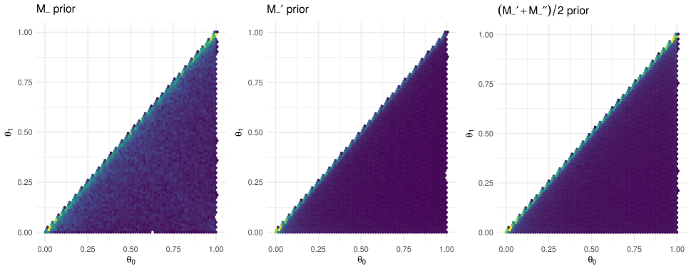
Figure 7: Left: heatmap of joint prior on $(\theta_{0},\theta_{1})$ implied by the $M_{-}$ prior (3.15) with $\mu_{0}=1/2,\mu_{e}=\mu_{s}=0.3,n_{0}=2,n_{e}=n_{s}=1$. Center: prior on $(\theta_{0},\theta_{1})$ under $M_{-}^{{}^{\prime}}$ with the same values of $(\mu_{0},\mu_{e},n_{0},n_{e})$. Right: prior on $(\theta_{0},\theta_{1})$ under the mixture model $(M_{-}^{{}^{\prime}}+M_{-}^{{}^{\prime\prime}})/2$ with $\mu_{1}=1/2,\mu_{s}^{\prime}=0.3,n_{1}=2,n_{s}^{\prime}=1$ and the same values of $(\mu_{0},\mu_{e},n_{0},n_{e})$.

Returning to the model $M_{-}^{{}^{\prime}}$ $(\ref{eq:m-'})$, some natural values for the prior hyperparameters are

$$\mu_{0}=\mu_{e}=1/2,\qquad n_{0}=n_{e}=2,$$

which define a flat $\text{Uniform}(0,1)^{2}$ prior on $(\theta_{0},\eta_{e})$. The resulting conditional prior on $\theta_{1}$ is

$$\theta_{1}|\theta_{0}\sim\text{Uniform}(0,\theta_{0}),$$

which presents an intuitive representation of the hypothesis $H_{-}:\theta_{1}<\theta_{0}$. Note, however, that this specification of the model handles $\theta_{0}$ as the baseline quantity. We can also go in the other direction, specifying priors on $\theta_{1}$ and the “side effects of placebo” $\eta_{s}^{\prime}$ and defining

$$\theta_{0}=\theta_{1}+(1-\theta_{1})\eta_{s}^{\prime},$$

which also instantiates $H_{-}:\theta_{1}<\theta_{0}$. We denote by $M_{-}^{{}^{\prime\prime}}$ the model

$$(\theta_{1},\eta_{s}^{\prime}) \sim\text{Beta}^{*}(\mu_{1},n_{1})\times\text{Beta}^{*}(\mu_{s}^{\prime},n_{s}^{\prime}),$$

$$\theta_{0} =\theta_{1}+(1-\theta_{1})\eta_{s}^{\prime}.$$

This asymmetry in our handling of $\theta_{0}$ and $\theta_{1}$ is reflected in the joint priors of $(\theta_{0},\theta_{1})$ under $M_{-}^{{}^{\prime}}$ and $M_{-}^{{}^{\prime\prime}}$. As the central panel of Figure 7 exhibits, the $M_{-}^{{}^{\prime}}$ joint prior tends to favor small proportions (whereas $M_{-}^{{}^{\prime\prime}}$, not plotted, favors large proportions). On the other hand, sampling $(\theta_{0},\eta_{e},\eta_{s})$ from the BREASE prior truncated to the set $\{(\theta_{0},\eta_{e},\eta_{s}):\theta_{1}<\theta_{0}\}$ (i.e., the $M_{-}$ prior (3.15)) yields a symmetric joint density on $(\theta_{0},\theta_{1})$ (left panel of Figure 7). To assuage this asymmetry, we can put $\theta_{0}$ and $\theta_{1}$ on equal footing when testing the one-sided hypothesis $H_{-}$ (and, similarly, $H_{+}$) by using a prior that averages those under $M_{-}^{{}^{\prime}}$ and $M_{-}^{{}^{\prime\prime}}$, as in the right panel of Figure 7. In practice, we can decompose $H_{-}$ into the submodels $M_{-}^{{}^{\prime}}$ and $M_{-}^{{}^{\prime\prime}}$ and report the marginal likelihood of $H_{-}$ as the average of the submodel marginal likelihoods. As the marginal likelihood under $M_{-}^{{}^{\prime\prime}}$ is also available analytically, this procedure comes with negligible added computational cost.

E.3 An empirical Bayes prior

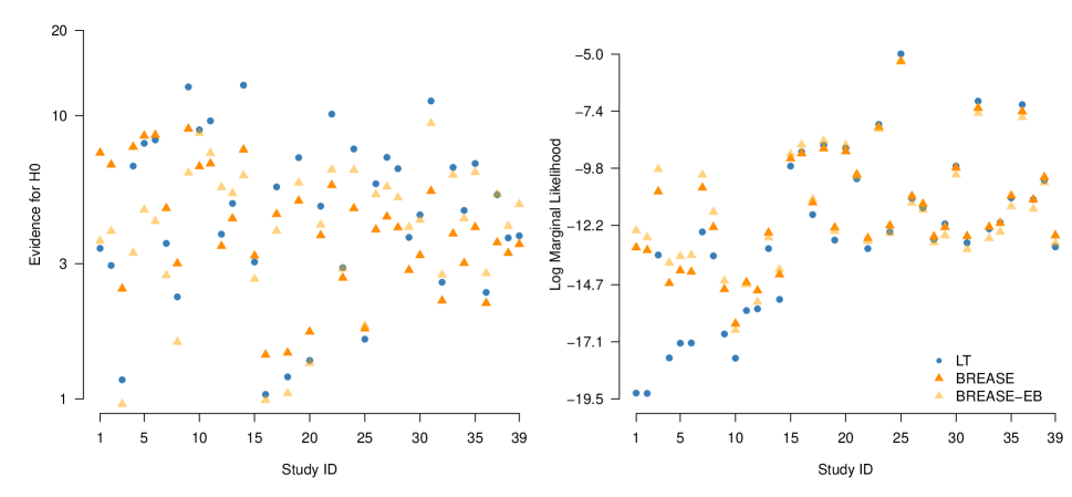
Figure 8: Comparison of Bayes factors ($\text{BF}_{01}$) and log marginal likelihoods under model $M_{1}$ (3.13) of the default LT, default BREASE, and empirical Bayes BREASE priors across the 39 NEJM studies.

As $\eta_{e}$ and $\eta_{s}$ are counterfactual probabilities, they are not generally point-identified from data. However, since $\theta_{0}$ and $\theta_{1}$ are identifiable, we can derive robust bounds on their range of possible values based on the observed data [107]. Equation (3.3) implies the following algebraic constraints on $\eta_{e}$ and $\eta_{s}$:

$$\max\left\{0,\frac{\theta_{0}-\theta_{1}}{\theta_{0}}\right\} \leq\eta_{e}\leq\min\left\{1,\frac{1-\theta_{1}}{\theta_{0}}\right\},$$ (E.3)

$$\max\left\{0,\frac{\theta_{1}-\theta_{0}}{1-\theta_{0}}\right\} \leq\eta_{s}\leq\min\left\{1,\frac{\theta_{1}}{1-\theta_{0}}\right\}.$$ (E.4)

The inequalities (E.3) and (E.4) define the (marginal) partially identified regions of $\eta_{e}$ and $\eta_{s}$, respectively. Denote these intervals by $I_{e}(\theta_{0},\theta_{1})=[\ell_{e}(\theta_{0},\theta_{1}),u_{e}(\theta_{0},\theta_{1})]$ and $I_{s}(\theta_{0},\theta_{1})=[\ell_{s}(\theta_{0},\theta_{1}),u_{s}(\theta_{0},\theta_{1})]$. In the limit of infinite data, the posterior mass of $\eta_{e}$ and $\eta_{s}$ will concentrate within $I_{e}(\theta_{0}^{*},\theta_{1}^{*})$ and $I_{s}(\theta_{0}^{*},\theta_{1}^{*})$, respectively, assuming $\theta_{0}^{*},\theta_{1}^{*}$ are the true values.

When conducting a Bayesian hypothesis test, a main concern is the sensitivity of Bayes factors to the prior. As demonstrated in Section 4, a prior that places unreasonable assumptions on the treatment effects can lead to questionable conclusions. In this light, it may be desired to take a data-driven approach to prior specification that concentrates prior mass near the partially identified intervals of $\eta_{e}$ and $\eta_{s}$. For example, we can set the prior means $\mu_{e}$ and $\mu_{s}$ to equal their midpoints:

$$\hat{\mu}_{e} =\frac{1}{2}\left(\ell_{e}(\hat{\theta}_{0},\hat{\theta}_{1})+u_{e}(\hat{\theta}_{0},\hat{\theta}_{1})\right),$$

$$\hat{\mu}_{s} =\frac{1}{2}\left(\ell_{s}(\hat{\theta}_{0},\hat{\theta}_{1})+u_{s}(\hat{\theta}_{0},\hat{\theta}_{1})\right),$$

where we use point estimates of the population proportions:

$$\hat{\theta}_{0} =\frac{y_{0}+1}{N_{0}+2},\qquad\hat{\theta}_{1}=\frac{y_{1}+1}{N_{1}+2}.$$

As $\hat{\theta}_{0}$ shrinks the sample proportion toward $1/2$, it avoids division by zero in (E.3) and (E.4). Hence, we might consider priors of the form $\text{BREASE}(1/2,\hat{\mu}_{e},\hat{\mu}_{s};2,n,n)$ with $n\geq 0$. As this prior is estimated from the observed data, it can be thought of as an empirical Bayes approach [95]. As such, we denote it by $\text{BREASE-EB}(n)$.

Note that when $n=1$ and $\hat{\theta}_{0}=\hat{\theta}_{1}=1/2$ (e.g., in the absence of data or when the sample proportions are $1/2$), we obtain a vague Jeffreys marginal prior $\text{Beta}(1/2,1/2)$ on $\eta_{e}$ and $\eta_{s}$. The choice of prior sample size $n=1$ yields something resembling a unit information prior [99], wherein the prior mean is estimated from data and its spread is chosen so that the information content of the prior matches that of a single observation.

Figure 8 compares Bayes factors ($\text{BF}_{01}$) and log marginal likelihoods under model $M_{1}$ (3.13) of the default $\text{LT}(0,0;1,1)$, $\text{BREASE}(1/2,0.3,0.3;2,1,1)$, and $\text{BREASE-EB}(1)$ priors across the 39 NEJM studies reporting null results. The BREASE and BREASE-EB priors tend to provide the most equivocal Bayes factors on average, with mean $\text{BF}_{01}$ equal to 4.41, 4.42, and 5.38 for the BREASE-EB, BREASE, and LT priors, respectively. However, BREASE-EB Bayes factors tend to be closer to those of the LT approach than the default BREASE prior, with mean absolute percentage differences from the LT $\text{BF}_{01}$ of 19% for the former and 32% for the latter.

Comparing log marginal likelihoods, which quantify the predictive performance of a model, we see that the BREASE-EB and default BREASE priors perform similarly, and generally better than the default LT prior, although the default BREASE performs slightly better overall. Indeed, the default BREASE log marginal likelihood exceeds the LT in 74% of the studies compared to 59% for the BREASE-EB prior. Furthermore, the default BREASE outperforms BREASE-EB in 62% of the studies.

Appendix F Bayes factors with the IB and LT approaches

Following [129], we calculate the Bayes factor $\text{BF}_{10}$ for the IB approach using the Savage-Dickey density ratio method applied to the difference of proportions $\eta=\theta_{0}-\theta_{1}$ [116]. A formula for the prior density of $\eta$ at the null $H_{0}:\eta=0$ can be found in Appendix A of [129]. The Bayes factor using the $\text{IB}((a,a),(a,a))$ prior under $H_{1}$ as described in Section 2.2.1 is then

$$\text{BF}_{10}=\frac{\text{B}(2a-1,2a-1)\text{B}(a+y_{0},a+N_{0}-y_{0})\text{B}(a+y_{1},a+N_{1}-y_{1})}{\text{B}(2a+y_{0}+y_{1}-1,2a+N_{0}-y_{0}+N_{1}-y_{1}-1)\text{B}(a,a)^{2}}.$$

Posterior estimates and credible intervals under $H_{1}$ are calculated using exact samples from the independent beta posterior.

Bayes factors $\text{BF}_{10}$ for the LT approach are calculating using the abtest package in R [127]. The package uses a Laplace approximation to calculate $\text{BF}_{10}$, which is shown to have good performance. The LT prior under $H_{1}$ is as described in Section 2.2.2. Under $H_{0}:\psi=0$, the prior is $\beta\sim\text{Normal}(\mu_{\beta},\sigma_{\beta})$ with default values $(\mu_{\beta},\sigma_{\beta})=(0,1)$. Posterior estimates and credible intervals under $H_{1}$ are calculated using posterior samples output by abtest. As abtest only reports marginal likelihoods up to a multiplicative constant, we used RJAGS [131] to generate MCMC samples from the LT posterior and THAMES [130] to estimate the LT marginal likelihood for Figure 5(b) using the samples.

References

- [1] Alan Agresti and David B. Hitchcock “Bayesian inference for categorical data analysis” In Statistical Methods and Applications 14.3, 2005, pp. 297–330
- [2] Alan Agresti and Yongyi Min “Frequentist Performance of Bayesian Confidence Intervals for Comparing Proportions in 2 × 2 Contingency Tables” In Biometrics 61.2, 2005, pp. 515–523
- [3] James H. Albert and Arjun K. Gupta “Bayesian Estimation Methods for 2 × 2 Contingency Tables Using Mixtures of Dirichlet Distributions” In Journal of the American Statistical Association 78.383, 1983, pp. 708–717
- [4] James H. Albert and Arjun K. Gupta “Bayesian methods for binomial data with applications to a nonresponse problem” In J. Amer. Statist. Assoc. 80, 1985, pp. 167–174
- [5] James H. Albert and Arjun K. Gupta “Estimation in contingency tables using prior information” In Journal of the Royal Statistical Society: Series B (Methodological) 45.1, 1983, pp. 60–69
- [6] James H. Albert and Arjun K. Gupta “Mixtures of Dirichlet Distributions and Estimation in Contingency Tables” In The Annals of Statistics 10.4, 1982, pp. 1261–1268
- [7] Gordon R. Antelman “Interrelated Bernoulli Processes” In Journal of the American Statistical Association 67.340, 1972, pp. 831–841
- [8] D. Basu and C.. B. Pereira “On the Bayesian analysis of categorical data: the problem of nonresponse” In J. Statist. Plann. Inference 6, 1982, pp. 345–362
- [9] Thomas Bayes “An essay toward solving a problem in the doctrine of chances, with Richard Price’s foreword and discussion” In Philos. Trans. R. Soc. London 53, 1763, pp. 370–418
- [10] AJ Branscum, IA Gardner and WO Johnson “Estimation of diagnostic-test sensitivity and specificity through Bayesian modeling” In Preventive veterinary medicine 68.2-4 Elsevier, 2005, pp. 145–163
- [11] Harlan Campbell and Paul Gustafson “Bayes Factors and Posterior Estimation: Two Sides of the Very Same Coin” In The American Statistician 0.0, 2022, pp. 1–11
- [12] George Casella and Elías Moreno “Assessing Robustness of Intrinsic Tests of Independence in Two-Way Contingency Tables” In Journal of the American Statistical Association 104.487, 2009, pp. 1261–1271
- [13] David M. Chickering and Judea Pearl “A Clinician’s Tool for Analyzing Non-compliance” In Proceedings of the AAAI Conference on Artificial Intelligence, 13, 1996
- [14] Carlos Cinelli and Judea Pearl “Generalizing experimental results by leveraging knowledge of mechanisms” In European Journal of Epidemiology 36 Springer, 2021, pp. 149–164
- [15] J.. Copas “Randomization models for the Matched and Unmatched 2 × 2 Tables” In Biometrika 60.3 [Oxford University Press, Biometrika Trust], 1973, pp. 467–476 URL: http://www.jstor.org/stable/2334995
- [16] Fabian Dablander et al. “A puzzle of proportions: Two popular Bayesian tests can yield dramatically different conclusions” In Statistics in Medicine 41.8, 2022, pp. 1319–1333
- [17] H.T. Davies, I.K. Crombie and M. Tavakoli “When can odds ratios mislead?” In BMJ 316.7136, 1998, pp. 989–991
- [18] J.. Dickey, J.. Jiang and J.. Kadane “Bayesian methods for censored categorical data” In Journal of the American Statistical Association 82, 1987, pp. 773–781
- [19] James M. Dickey “Multiple Hypergeometric Functions: Probabilistic Interpretations and Statistical Uses” In Journal of the American Statistical Association 78.383, 1983, pp. 628–637
- [20] James M. Dickey and B.. Lientz “The Weighted Likelihood Ratio, Sharp Hypotheses about Chances, the Order of a Markov Chain” In The Annals of Mathematical Statistics 41.1, 1970, pp. 214–226
- [21] Peng Ding and Luke W. Miratrix “Model-free causal inference of binary experimental data” In Scandinavian Journal of Statistics 46.1, 2019, pp. 200–214
- [22] Michael Evans and Hadas Moshonov “Checking for Prior-Data Conflict” In Bayesian Analysis 1.4, 2006, pp. 893–914
- [23] Andrew Gelman, John B Carlin, Hal S Stern and Donald B Rubin “Bayesian data analysis” ChapmanHall/CRC, 1995
- [24] Sander Greenland and James Robins “Identifiability, Exchangeability, and Epidemiological Confounding” In International Journal of Epidemiology 15.3, 1986, pp. 413–419
- [25] Quentin F. Gronau, K.. Raj and Eric-Jan Wagenmakers “Informed Bayesian Inference for the A/B Test” In Journal of Statistical Software 100.17, 2021, pp. 1–39
- [26] E. Gunel “A Bayesian analysis of the multinomial model for a dichotomous response with nonrespondents” In Comm. Statist. Theory Methods 13, 1984, pp. 737–751
- [27] Erdogan Gunel and James Dickey “Bayes Factors for Independence in Contingency Tables” In Biometrika 61.3, 1974, pp. 545–557
- [28] Paul Gustafson “Bayesian inference for partially identified models: Exploring the limits of limited data” CRC Press, 2015
- [29] Keisuke Hirano, Guido W Imbens, Donald B Rubin and Xiao-Hua Zhou “Assessing the effect of an influenza vaccine in an encouragement design” In Biostatistics 1.1 Oxford University Press, 2000, pp. 69–88
- [30] Guido W. Imbens and Donald B. Rubin “Bayesian Inference for Causal Effects in Randomized Experiments with Noncompliance” In The Annals of Statistics 25.1, 1997, pp. 305–327
- [31] Harold Jeffreys “Some Tests of Significance, Treated by the Theory of Probability” In Mathematical Proceedings of the Cambridge Philosophical Society 31.2, 1935, pp. 203–222
- [32] Harold Jeffreys “Theory of Probability” Oxford, UK: Oxford University Press, 1961
- [33] M.J. Karson and W.J. Wrobleski “A Bayesian Analysis of a Binomial Model with a Partially Informative Category” In Proceedings of the Business and Economic Statistics Section, American Statistical Association, 1970, pp. 532–534
- [34] Robert E. Kass and Adrian E. Raftery “Bayes Factors” In Journal of the American Statistical Association 90.430, 1995, pp. 773–795
- [35] Robert E. Kass and Suresh K. Vaidyanathan “Approximate Bayes Factors and Orthogonal Parameters, with Application to Testing Equality of Two Binomial Proportions” In Journal of the Royal Statistical Society. Series B (Methodological) 54.1, 1992, pp. 129–144
- [36] Robert E. Kass and Larry Wasserman “A Reference Bayesian Test for Nested Hypotheses and its Relationship to the Schwarz Criterion” In Journal of the American Statistical Association 90.431, 1995, pp. 928–934
- [37] G.. Kaufman and Benjamin King “A Bayesian Analysis of Nonresponse in Dichotomous Processes” In Journal of the American Statistical Association 68.343, 1973, pp. 670–678
- [38] Ruth A. Killion and Douglas A. Zahn “A Bibliography of Contingency Table Literature: 1900 to 1974” In International Statistical Review 44.1, 1976, pp. 71–112
- [39] John Kruschke “Doing Bayesian Data Analysis: A Tutorial with R, JAGS, and Stan” In Doing Bayesian Data Analysis Elsevier Science & Technology, 2014
- [40] Pierre Simon Laplace “Mémoire sur la probabilité de causes par les évenements” In Mémoire de l’académie royale des sciences, 1774
- [41] Edward E. Leamer “Specification searches: ad hoc inference with nonexperimental data” In Specification searches: ad hoc inference with nonexperimental data, Wiley series in probability and mathematical statistics New York: Wiley, 1978
- [42] Tom Leonard “Bayesian estimation methods for two-way contingency tables” In Journal of the Royal Statistical Society: Series B (Methodological) 37.1, 1975, pp. 23–37
- [43] Tom Leonard “Bayesian Methods for Binomial Data” In Biometrika 59.3, 1972, pp. 581–589
- [44] David Madigan “Bayesian graphical models, intention-to-treat, and the Rubin causal model” In Seventh International Workshop on Artificial Intelligence and Statistics, 1999 PMLR
- [45] Richard McElreath “Statistical rethinking : a Bayesian course with examples in R and Stan” In Statistical rethinking: a Bayesian course with examples in R and Stan, Texts in statistical science Chapman & Hall/CRC, 2020
- [46] Martin Metodiev et al. “Easily Computed Marginal Likelihoods from Posterior Simulation Using the THAMES Estimator”, 2023 arXiv:2305.08952 [stat.ME]
- [47] Jerzy Neyman “On the Application of Probability Theory to Agricultural Experiments. Essay on Principles. Section 9.” Translated from the 1923 Polish original and edited by D. M. Dabrowska and T. P. Speed In Statistical Science 5.4, 1990, pp. 465–472
- [48] Kai Wang Ng, Man-Lai Tang, Ming Tan and Guo-Liang Tian “Grouped Dirichlet distribution: A new tool for incomplete categorical data analysis” In Journal of Multivariate Analysis 99.3, 2008, pp. 490–509
- [49] Kai Wang Ng, Guo-Liang Tian and Man-Lai Tang “Dirichlet and related distributions: Theory, methods and applications” Wiley, 2011
- [50] T. Park and M.. Brown “Models for categorical data with nonignorable nonresponse” In J. Amer. Statist. Assoc. 89, 1994, pp. 44–52
- [51] Judea Pearl “Causality” Cambridge University Press, 2009
- [52] T. Pham-Gia and N. Turkkan “Distribution of the linear combination of two general beta variables and applications” In Communications in Statistics - Theory and Methods 27.7, 1998, pp. 1851–1869
- [53] Steering Committee Physicians’ Health Study Research Group “Final Report on the Aspirin Component of the Ongoing Physicians’ Health Study” In New England Journal of Medicine 321.3, 1989, pp. 129–135
- [54] Martyn Plummer “rjags: Bayesian Graphical Models using MCMC” R package version 4-14, 2023
- [55] Fernando P. Polack et al. “Safety and Efficacy of the BNT162b2 mRNA Covid-19 Vaccine” In New England Journal of Medicine 383.27, 2020, pp. 2603–2615
- [56] Thomas S. Richardson, Robin J. Evans and James M. Robins “Transparent Parametrizations of Models for Potential Outcomes” In Bayesian Statistics 9 Oxford, UK: Oxford University Press, 2011
- [57] Herbert E. Robbins “An Empirical Bayes Approach to Statistics” In Breakthroughs in Statistics: Foundations and Basic Theory New York, NY: Springer New York, 1992, pp. 388–394
- [58] Donald B Rubin “Estimating causal effects of treatments in randomized and nonrandomized studies.” In Journal of educational Psychology 66.5 American Psychological Association, 1974, pp. 688
- [59] Silas W Smith, Manfred Hauben and Jeffrey K Aronson “Paradoxical and bidirectional drug effects” In Drug safety 35 Springer, 2012, pp. 173–189
- [60] M.. Springer and W.. Thompson “The Distribution of Products of Beta, Gamma and Gaussian Random Variables” In SIAM Journal on Applied Mathematics 18.4 Society for IndustrialApplied Mathematics, 1970, pp. 721–737
- [61] Stan Development Team “RStan: the R interface to Stan” R package version 2.21.8, 2023
- [62] Peter F Thall, Richard M Simon and Elihu H Estey “Bayesian sequential monitoring designs for single-arm clinical trials with multiple outcomes” In Statistics in medicine 14.4 Wiley Online Library, 1995, pp. 357–379
- [63] Guo-Liang Tian, Kai Wang Ng and Zhi Geng “Bayesian computation for contingency tables with incomplete cell-counts” In Statistica Sinica 13.1, 2003, pp. 189–206
- [64] Jin Tian and Judea Pearl “Probabilities of causation: Bounds and identification” In Annals of Mathematics and Artificial Intelligence 28.1 Institute of Mathematical Statistics, 2000, pp. 287–313
- [65] U.S. Food and Drug Administration “Guidance for industry: emergency use authorization for vaccines to prevent COVID-19”, 2020 URL: https://www.fda.gov/media/142749/download
- [66] Eric-Jan Wagenmakers, Tom Lodewyckx, Himanshu Kuriyal and Raoul Grasman “Bayesian hypothesis testing for psychologists: A tutorial on the Savage–Dickey method” In Cognitive Psychology 60.3, 2010, pp. 158–189
- [67] Thomas Bayes “An essay toward solving a problem in the doctrine of chances, with Richard Price’s foreword and discussion” In Philos. Trans. R. Soc. London 53, 1763, pp. 370–418
- [68] Pierre Simon Laplace “Mémoire sur la probabilité de causes par les évenements” In Mémoire de l’académie royale des sciences, 1774
- [69] Harold Jeffreys “Some Tests of Significance, Treated by the Theory of Probability” In Mathematical Proceedings of the Cambridge Philosophical Society 31.2, 1935, pp. 203–222
- [70] Harold Jeffreys “Theory of Probability” Oxford, UK: Oxford University Press, 1961
- [71] James M. Dickey and B.. Lientz “The Weighted Likelihood Ratio, Sharp Hypotheses about Chances, the Order of a Markov Chain” In The Annals of Mathematical Statistics 41.1, 1970, pp. 214–226
- [72] M.J. Karson and W.J. Wrobleski “A Bayesian Analysis of a Binomial Model with a Partially Informative Category” In Proceedings of the Business and Economic Statistics Section, American Statistical Association, 1970, pp. 532–534
- [73] M.. Springer and W.. Thompson “The Distribution of Products of Beta, Gamma and Gaussian Random Variables” In SIAM Journal on Applied Mathematics 18.4 Society for IndustrialApplied Mathematics, 1970, pp. 721–737
- [74] Gordon R. Antelman “Interrelated Bernoulli Processes” In Journal of the American Statistical Association 67.340, 1972, pp. 831–841
- [75] Tom Leonard “Bayesian Methods for Binomial Data” In Biometrika 59.3, 1972, pp. 581–589
- [76] J.. Copas “Randomization models for the Matched and Unmatched 2 × 2 Tables” In Biometrika 60.3 [Oxford University Press, Biometrika Trust], 1973, pp. 467–476 URL: http://www.jstor.org/stable/2334995
- [77] G.. Kaufman and Benjamin King “A Bayesian Analysis of Nonresponse in Dichotomous Processes” In Journal of the American Statistical Association 68.343, 1973, pp. 670–678
- [78] Erdogan Gunel and James Dickey “Bayes Factors for Independence in Contingency Tables” In Biometrika 61.3, 1974, pp. 545–557
- [79] Donald B Rubin “Estimating causal effects of treatments in randomized and nonrandomized studies.” In Journal of educational Psychology 66.5 American Psychological Association, 1974, pp. 688
- [80] Tom Leonard “Bayesian estimation methods for two-way contingency tables” In Journal of the Royal Statistical Society: Series B (Methodological) 37.1, 1975, pp. 23–37
- [81] Ruth A. Killion and Douglas A. Zahn “A Bibliography of Contingency Table Literature: 1900 to 1974” In International Statistical Review 44.1, 1976, pp. 71–112
- [82] Edward E. Leamer “Specification searches: ad hoc inference with nonexperimental data” In Specification searches: ad hoc inference with nonexperimental data, Wiley series in probability and mathematical statistics New York: Wiley, 1978
- [83] James H. Albert and Arjun K. Gupta “Mixtures of Dirichlet Distributions and Estimation in Contingency Tables” In The Annals of Statistics 10.4, 1982, pp. 1261–1268
- [84] D. Basu and C.. B. Pereira “On the Bayesian analysis of categorical data: the problem of nonresponse” In J. Statist. Plann. Inference 6, 1982, pp. 345–362
- [85] James H. Albert and Arjun K. Gupta “Bayesian Estimation Methods for 2 × 2 Contingency Tables Using Mixtures of Dirichlet Distributions” In Journal of the American Statistical Association 78.383, 1983, pp. 708–717
- [86] James H. Albert and Arjun K. Gupta “Estimation in contingency tables using prior information” In Journal of the Royal Statistical Society: Series B (Methodological) 45.1, 1983, pp. 60–69
- [87] James M. Dickey “Multiple Hypergeometric Functions: Probabilistic Interpretations and Statistical Uses” In Journal of the American Statistical Association 78.383, 1983, pp. 628–637
- [88] E. Gunel “A Bayesian analysis of the multinomial model for a dichotomous response with nonrespondents” In Comm. Statist. Theory Methods 13, 1984, pp. 737–751
- [89] James H. Albert and Arjun K. Gupta “Bayesian methods for binomial data with applications to a nonresponse problem” In J. Amer. Statist. Assoc. 80, 1985, pp. 167–174
- [90] Sander Greenland and James Robins “Identifiability, Exchangeability, and Epidemiological Confounding” In International Journal of Epidemiology 15.3, 1986, pp. 413–419
- [91] J.. Dickey, J.. Jiang and J.. Kadane “Bayesian methods for censored categorical data” In Journal of the American Statistical Association 82, 1987, pp. 773–781
- [92] Steering Committee Physicians’ Health Study Research Group “Final Report on the Aspirin Component of the Ongoing Physicians’ Health Study” In New England Journal of Medicine 321.3, 1989, pp. 129–135
- [93] Jerzy Neyman “On the Application of Probability Theory to Agricultural Experiments. Essay on Principles. Section 9.” Translated from the 1923 Polish original and edited by D. M. Dabrowska and T. P. Speed In Statistical Science 5.4, 1990, pp. 465–472
- [94] Robert E. Kass and Suresh K. Vaidyanathan “Approximate Bayes Factors and Orthogonal Parameters, with Application to Testing Equality of Two Binomial Proportions” In Journal of the Royal Statistical Society. Series B (Methodological) 54.1, 1992, pp. 129–144
- [95] Herbert E. Robbins “An Empirical Bayes Approach to Statistics” In Breakthroughs in Statistics: Foundations and Basic Theory New York, NY: Springer New York, 1992, pp. 388–394
- [96] T. Park and M.. Brown “Models for categorical data with nonignorable nonresponse” In J. Amer. Statist. Assoc. 89, 1994, pp. 44–52
- [97] Andrew Gelman, John B Carlin, Hal S Stern and Donald B Rubin “Bayesian data analysis” ChapmanHall/CRC, 1995
- [98] Robert E. Kass and Adrian E. Raftery “Bayes Factors” In Journal of the American Statistical Association 90.430, 1995, pp. 773–795
- [99] Robert E. Kass and Larry Wasserman “A Reference Bayesian Test for Nested Hypotheses and its Relationship to the Schwarz Criterion” In Journal of the American Statistical Association 90.431, 1995, pp. 928–934
- [100] Peter F Thall, Richard M Simon and Elihu H Estey “Bayesian sequential monitoring designs for single-arm clinical trials with multiple outcomes” In Statistics in medicine 14.4 Wiley Online Library, 1995, pp. 357–379
- [101] David M. Chickering and Judea Pearl “A Clinician’s Tool for Analyzing Non-compliance” In Proceedings of the AAAI Conference on Artificial Intelligence, 13, 1996
- [102] Guido W. Imbens and Donald B. Rubin “Bayesian Inference for Causal Effects in Randomized Experiments with Noncompliance” In The Annals of Statistics 25.1, 1997, pp. 305–327
- [103] H.T. Davies, I.K. Crombie and M. Tavakoli “When can odds ratios mislead?” In BMJ 316.7136, 1998, pp. 989–991
- [104] T. Pham-Gia and N. Turkkan “Distribution of the linear combination of two general beta variables and applications” In Communications in Statistics - Theory and Methods 27.7, 1998, pp. 1851–1869
- [105] David Madigan “Bayesian graphical models, intention-to-treat, and the Rubin causal model” In Seventh International Workshop on Artificial Intelligence and Statistics, 1999 PMLR
- [106] Keisuke Hirano, Guido W Imbens, Donald B Rubin and Xiao-Hua Zhou “Assessing the effect of an influenza vaccine in an encouragement design” In Biostatistics 1.1 Oxford University Press, 2000, pp. 69–88
- [107] Jin Tian and Judea Pearl “Probabilities of causation: Bounds and identification” In Annals of Mathematics and Artificial Intelligence 28.1 Institute of Mathematical Statistics, 2000, pp. 287–313
- [108] Guo-Liang Tian, Kai Wang Ng and Zhi Geng “Bayesian computation for contingency tables with incomplete cell-counts” In Statistica Sinica 13.1, 2003, pp. 189–206
- [109] Alan Agresti and David B. Hitchcock “Bayesian inference for categorical data analysis” In Statistical Methods and Applications 14.3, 2005, pp. 297–330
- [110] Alan Agresti and Yongyi Min “Frequentist Performance of Bayesian Confidence Intervals for Comparing Proportions in 2 × 2 Contingency Tables” In Biometrics 61.2, 2005, pp. 515–523
- [111] AJ Branscum, IA Gardner and WO Johnson “Estimation of diagnostic-test sensitivity and specificity through Bayesian modeling” In Preventive veterinary medicine 68.2-4 Elsevier, 2005, pp. 145–163
- [112] Michael Evans and Hadas Moshonov “Checking for Prior-Data Conflict” In Bayesian Analysis 1.4, 2006, pp. 893–914
- [113] Kai Wang Ng, Man-Lai Tang, Ming Tan and Guo-Liang Tian “Grouped Dirichlet distribution: A new tool for incomplete categorical data analysis” In Journal of Multivariate Analysis 99.3, 2008, pp. 490–509
- [114] George Casella and Elías Moreno “Assessing Robustness of Intrinsic Tests of Independence in Two-Way Contingency Tables” In Journal of the American Statistical Association 104.487, 2009, pp. 1261–1271
- [115] Judea Pearl “Causality” Cambridge University Press, 2009
- [116] Eric-Jan Wagenmakers, Tom Lodewyckx, Himanshu Kuriyal and Raoul Grasman “Bayesian hypothesis testing for psychologists: A tutorial on the Savage–Dickey method” In Cognitive Psychology 60.3, 2010, pp. 158–189
- [117] Kai Wang Ng, Guo-Liang Tian and Man-Lai Tang “Dirichlet and related distributions: Theory, methods and applications” Wiley, 2011
- [118] Thomas S. Richardson, Robin J. Evans and James M. Robins “Transparent Parametrizations of Models for Potential Outcomes” In Bayesian Statistics 9 Oxford, UK: Oxford University Press, 2011
- [119] Silas W Smith, Manfred Hauben and Jeffrey K Aronson “Paradoxical and bidirectional drug effects” In Drug safety 35 Springer, 2012, pp. 173–189
- [120] John Kruschke “Doing Bayesian Data Analysis: A Tutorial with R, JAGS, and Stan” In Doing Bayesian Data Analysis Elsevier Science & Technology, 2014
- [121] Paul Gustafson “Bayesian inference for partially identified models: Exploring the limits of limited data” CRC Press, 2015
- [122] Peng Ding and Luke W. Miratrix “Model-free causal inference of binary experimental data” In Scandinavian Journal of Statistics 46.1, 2019, pp. 200–214
- [123] Richard McElreath “Statistical rethinking : a Bayesian course with examples in R and Stan” In Statistical rethinking: a Bayesian course with examples in R and Stan, Texts in statistical science Chapman & Hall/CRC, 2020
- [124] Fernando P. Polack et al. “Safety and Efficacy of the BNT162b2 mRNA Covid-19 Vaccine” In New England Journal of Medicine 383.27, 2020, pp. 2603–2615
- [125] U.S. Food and Drug Administration “Guidance for industry: emergency use authorization for vaccines to prevent COVID-19”, 2020 URL: https://www.fda.gov/media/142749/download
- [126] Carlos Cinelli and Judea Pearl “Generalizing experimental results by leveraging knowledge of mechanisms” In European Journal of Epidemiology 36 Springer, 2021, pp. 149–164
- [127] Quentin F. Gronau, K.. Raj and Eric-Jan Wagenmakers “Informed Bayesian Inference for the A/B Test” In Journal of Statistical Software 100.17, 2021, pp. 1–39
- [128] Harlan Campbell and Paul Gustafson “Bayes Factors and Posterior Estimation: Two Sides of the Very Same Coin” In The American Statistician 0.0, 2022, pp. 1–11
- [129] Fabian Dablander et al. “A puzzle of proportions: Two popular Bayesian tests can yield dramatically different conclusions” In Statistics in Medicine 41.8, 2022, pp. 1319–1333
- [130] Martin Metodiev et al. “Easily Computed Marginal Likelihoods from Posterior Simulation Using the THAMES Estimator”, 2023 arXiv:2305.08952 [stat.ME]
- [131] Martyn Plummer “rjags: Bayesian Graphical Models using MCMC” R package version 4-14, 2023
- [132] Stan Development Team “RStan: the R interface to Stan” R package version 2.21.8, 2023
Appendix for