Higher Derivative Sigma Models

Abstract

We explore the nature of running couplings in the higher derivative linear and nonlinear sigma models and show that the results in dimensional regularization for the physical running couplings do not always match the values quoted in the literature. Heat kernel methods identify divergences correctly, but not all of these divergences are related to physical running couplings. Likewise the running found using the Functional Renormalization Group does not always appear as running couplings in physical processes, even for the case of logarithmic running. The basic coupling of the higher derivative SU(N) nonlinear sigma model does not run at all at one loop, in contrast to published claims for asymptotic freedom. At one loop we describe how to properly identify the physical running couplings in these theories, and provide revised numbers for the higher derivative nonlinear sigma model.

I Introduction

We use running coupling constants routinely in quantum field theory. By defining a scale dependent coupling constant one can sum up a set of quantum corrections which appear at that scale. The use of the running coupling constant in physical reactions yields a better perturbative expansion at that scale than does using a coupling defined at very distant scales.

The running couplings are universal because they are tied to the renormalization of the bare couplings. In standard renormalizable theories the running is always logarithmic in the energy scales. There are a set of techniques which are used to calculate the beta functions for the couplings which exploit this connection to the divergences of the theory.

The goal of the present paper is to illustrate how some of these techniques no longer yield physical running couplings when applied to theories which involve higher derivatives, and to propose a solution. This problem has been identified and studied in detail in a simple model in recent work by Buccio, Percacci and one of present authors Buccio:2023lzo , and we also review that example in Section III. We motivate such theories in the next subsection. However, first we describe the general reasons why the calculations in the literature for such theories do not yield physical scale dependent running couplings.

I.1 Identifying running couplings

Let us start off with what appears to be a curiosity. In theories which include four derivatives in the kinetic energy, the propagator falls as $1/p^{4}$. In calculations, one often encounters the tadpole diagram of Fig 1. This integral is logarithmically divergent, with

$$I_{\text{tad}}=-i\int d^{4}p\frac{1}{p^{4}}\sim\log\frac{\Lambda^{2}}{k^{2}}~{}~{}~{}~{}~{}~{}~{}~{}~{}~{}{\rm(UV/IR~{}cutoffs)}$$ (1)

where $\Lambda$ is a UV cutoff and $k$ is an IR cutoff. However, in dimensional regularization this integral is scaleless and vanishes

$$I_{\text{tad}}=-i\int d^{d}p\frac{1}{p^{4}}=0~{}~{}~{}~{}~{}~{}~{}~{}~{}~{}~{}~{}~{}~{}~{}~{}~{}{\rm(dimensional~{}regularization)}\ \ .$$ (2)

This is a well-known oddity of dimensional regularization, here applied to quartic propagators. Despite this difference there is no disagreement in physical processes, which are all independent of the regularization scheme. The $\log\Lambda/k$ factor disappears in the renormalization process and does not lead to any physical effects.

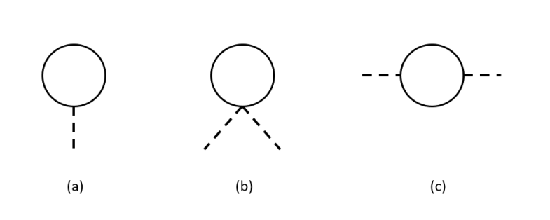
Figure 1: Diagrams (a) and (b) and referred to as tadpole diagrams, with any number of external legs. Diagram (c) is a bubble diagram. The important distinction is whether the external momentum flows through the loop or not.

However, this curiosity does have important consequences for the calculation of beta functions. With cutoff regularization, we often calculate the beta function using $\Lambda d/d\Lambda$ on the relevant quantum corrections. The Functional Renormalization Group, as applied in the Asymptotic Safety program, uses the infrared cutoff dependence $kd/dk$. However, the vanishing of the purely quartic integral, Eq. 2, already tells us that this must be wrong - the tadpole integral cannot lead to running couplings if the integral vanishes. This can be understood physically because no external momentum flows through the tadpole integral. The whole integral is just a constant which is absorbed into the renormalization of the parameter and there is no residual dependence on the energy scale. Identifying $\log\Lambda^{2}$, $\log k^{2}$ (or $\log\mu^{2}$ in dimensional regularization) does not tell us about $\log E^{2}$, where $E$ represents the energy scale of whatever reaction which we are studying. We will show that this distinction has created errors in the calculation of the physical beta functions which exist in the literature.

More generally, identifying the divergences is not sufficient in cases where there are other dimensionful parameters. This issue is not just the presence of tadpole diagrams themselves, as the scalar tadpole integral also arises in the Passarino-Veltman reduction of general bubble, triangle, box, etc., diagrams. One must separate the $\log E^{2}/\mu^{2}$ factors from the $\log m^{2}/\mu^{2}$ ones. Heat kernel methods are good at identifying the divergences but do not tell us the form of the logarithms. There needs to be an extra step to identify which divergences are associated with kinematic logarithms and we will provide this separation in Sect. V. This issue surfaces in various ways in the theories described in this paper, and also more widely in the literature.

There is an additional feature that the form of the running couplings changes between the low energy and high energy regions. In theories with higher derivatives, there is a mass scale, simply called $m$ in this paper, related to the relative size of the two derivative and four derivative kinetic energy terms. Here low energy refers to $E<m$ and high energy to $E>m$. At low energy the running couplings can be found by Effective Field Theory (EFT) methods. The high energy region requires the full theory. Standard methods may capture one or the other of these, and again one needs extra work to separate the divergences from the kinematic running. In some theories there is a hierarchy of effective field theories.

We will see that in the higher derivative linear sigma model of Section II, the coupling $\lambda$ runs at low energy but does not run at high energy. In the nonlinear version studied in Sec. III, the basic coupling $g$ does not run in the EFT region, but does run at high energy. In the SU(N) nonlinear of Sec. IV, the basic coupling $f$ does not run at any scale, while the others run both below and above $m$, but with different values. We describe how to sort this out in general in Sec. V.

I.2 Theories with higher derivatives

In the space of possible quantum field theories, we normally limit ourselves to the sector with only two derivatives in the kinetic energy terms. However, there can be reasons for going beyond this limitation.

Lee and Wick explored higher derivative theories in order to have finite quantum field theories, without the usual divergences Lee:1970iw . The higher derivative kinetic energies improves the high energy behavior of propagators and perturbatively gives finite loop corrections for theories such as QED. For a similar reason, extra derivative kinetic energies can also turn non-renormalizable theories into renormalizable ones. Here the example with the greatest physical interest is gravity. General relativity by itself is non-renormalizable but when terms proportional to the curvature squared are included – bringing in four derivatives – the resulting theory of Quadratic Gravity is renormalizable Stelle:1976gc ; Salvio:2018crh ; Donoghue:2021cza .

Higher derivative operators can also be generated by quantum corrections. When treated as simple perturbations using effective field theory techniques the propagators can remain the same as in the original theory. However, in some settings all the higher order operators are on the same footing. For example, with Functional Renormalization Group (FRG) techniques Dupuis:2020fhh ; Saueressig:2023irs one in principle includes all local operators, with scale transformations yielding a renormalization group flow of the couplings of these operators. Such techniques will always face the situation with higher derivative kinetic energies. The present practice of Asymptotic Safety most often treats gravity using FRG techniques Niedermaier:2006wt ; Reuter:2019byg .

Sigma models are an ideal testing ground for this class of theories. They are simple enough that one can focus on the essential new physics without too much complication. The SU(N) higher derivative nonlinear sigma model is the closest analogy to Quadratic Gravity as it shares all of the higher derivative features, but does not have the subtle feature of general coordinate invariance. The running of the couplings has been studied by Hasenfratz Hasenfratz:1988rf , and it has also been treated using FRG techniques by Percacci and Zanusso Percacci:2009fh , with results which agree within the appropriate limit. However those results differ from the physical running we find below. Moreover higher derivative sigma models are potentially useful because that can be simulated using lattice methods.

Higher derivative theories have features which differ from conventional QFT, and these are much debated in the literature. We have reviewed our own studies in Donoghue:2021cza . In the present paper we do not address these other aspects, but focus uniquely on the issue of renormalization group flow.

II The higher derivative linear sigma model

The higher derivative $O(N)$ linear sigma model is defined by the Lagrangian

$${\cal L}=\frac{1}{2}\partial_{\mu}\bm{\phi}\cdot\partial^{\mu}\bm{\phi}-\frac{1}{2m^{2}}\Box\bm{\phi}\cdot\Box\bm{\phi}+\frac{\mu_{0}^{2}}{2}\bm{\phi}\cdot\bm{\phi}-\frac{\lambda}{4}(\bm{\phi}\cdot\bm{\phi})^{2}\ \ .$$ (3)

Here the field $\bm{\phi}=\{\phi_{1},...,\phi_{N}\}$ is conventionally normalized and the higher derivative kinetic energy is parameterized by the mass $m$. Symmetry breaking takes place as normal, with the vacuum expectation value $v=\sqrt{\mu_{0}^{2}/\lambda}$, a heavy scalar with mass $m_{\sigma}^{2}=2\mu_{0}^{2}$ and $N-1$ Goldstone bosons. The higher derivative term implies extra massive degrees of freedom, even for the Goldstones whose propagator is

$$D_{F}(p)=\frac{1}{p^{2}-\frac{p^{4}}{m^{2}}}=\frac{1}{p^{2}}-\frac{1}{p^{2}-m^{2}}$$ (4)

The negative norm of the massive state is a well-known feature of higher derivative theories. For us the main feature is that it causes cancellations within loop integrals.

This theory is renormalizable. Because the higher derivative term improves the UV convergence, and the normal sigma model is already renormalizable, one might expect that the higher derivative version would actually be finite. However, the mass term in the theory, $\mu_{0}^{2}$, rather famously has a quadratic divergence, and the higher derivative modification merely reduces that to a logarithmic divergence. There are no divergences related to the quartic coupling $\lambda$.

Jansen, Kuti and Liu have explored a very similar model model both analytically and numerically as a probe of naturalness in the Higgs sector Jansen:1992xv ; Jansen:1993ji . Their model involves a yet higher derivative kinetic energy, $\phi\Box^{3}\phi$, such that the theory is finite rather than renormalizable. Nevertheless, the results described below for the running of $\lambda$ is present in their work. Our discussion highlights those features relevant for the remaining sections of this paper.

II.1 Renormalization without running

The divergence in the mass term comes from the tadpole diagram in Figure 1. The full evaluation of this tadpole reveals more about the physics that was not evident in our motivation section of Eq. 1 and Eq. 2. That is, even in cases where the tadpole diagram does not vanish, it still does not lead to running couplings.

A quadratic term in the propagator acts as an infrared cutoff in the tadpole integral. In contrast with the pure quartic integral of Eq. 2 the result now does not vanish. One finds

$$\delta m_{\sigma}^{2}={(N+2)\lambda}\tilde{I}_{tad}$$ (5)

with

$$\tilde{I}_{tad}=-i\int\frac{d^{d}p}{(2\pi)^{d}}\frac{1}{p^{2}-\frac{p^{4}}{m^{2}}} = -i\int\frac{d^{d}p}{(2\pi)^{d}}\left[\frac{1}{p^{2}}-\frac{1}{p^{2}-m^{2}}\right]$$ (6)

$$= -\frac{m^{2}}{16\pi^{2}}\left[\frac{1}{\epsilon}+\log 4\pi-\gamma-\log\left(\frac{m^{2}}{\mu^{2}}\right)+1\right]\ \ .$$

with $\epsilon=2/(4-d)$. (For the rest of the paper, unless noted we display only the divergences and the logarithms and suppress the remaining constants.)

Often when using dimensional regularization one follows the $1/\epsilon$ factors or equivalently uses $\mu\frac{d}{d\mu}$. Despite the divergence and the factor of $\log\mu^{2}$, this does not lead to a running mass. This is seen from the fact that the logarithm involves $\log m^{2}/\mu^{2}$ and not any kinematic quantity. After renormalization,

$$m_{\sigma,{\rm ren}}^{2}=m_{\sigma,{\rm bare}}+\delta m_{\sigma}^{2}$$ (7)

there is no residual dependence on any external scale. Measurement of the mass term at any scale will yield the same value. Using the $\log\mu$ dependence to define a running coupling would be incorrect.

II.2 Running without renormalization

The quantum corrections to the quartic coupling $\lambda$ do not involve any divergences. However, as first noted by Jansen, Kuti and Liu, the coupling has the interesting feature of running at low energies, and then the beta function vanishes at high energies. Our discussion here is appropriate for the unbroken phase at energies above the scale of symmetry breaking. For an analysis of the broken phase, see Section III.

The one loop correction to this coupling involves the scalar bubble diagram. Using the partial fraction decomposition of the propagator one readily finds that the scalar bubble integrals involve

$${\hat{I}}(q)=\left[I_{2}(0,0,q)-2I_{2}(0,m,q)+I_{2}(m,m,q)\right]$$ (8)

where the bubble integral is

$$I_{2}(m_{1},m_{2},q)=\frac{1}{16\pi^{2}}\left[\frac{1}{\epsilon}-\int dx\log\left(\frac{xm_{1}^{2}+(1-x)m_{2}^{2}-q^{2}x(1-x)}{\mu^{2}}\right)\right]\ \ .$$ (9)

One sees that the divergences and $\mu$ dependences cancel in ${\hat{I}}(q)$. Nevertheless, the result carries a logarithmic momentum dependence at low energy

$${\hat{I}}(q)=-\frac{1}{16\pi^{2}}\log(-q^{2}/m^{2})+...~{}~{}~{}~{}~{}~{},~{}(q^{2}\ll m^{2})$$ (10)

that leads to a running coupling. One finds the scattering amplitude for $\phi_{1}+\phi_{1}\to\phi_{1}+\phi_{1}$ to be

$${\cal M}=6\lambda\left[1-\lambda\frac{(N+8)}{3}\left({\hat{I}}(s)+{\hat{I}}(t)+{\hat{I}}(u)\right)\right]$$ (11)

When measuring the coupling in the scattering amplitude using the renormalization point $s=t=u=\mu_{R}^{2}\ll m^{2}$, the physical beta function

$$\beta_{\lambda}=\mu_{R}\frac{\partial}{\partial\mu_{R}}\lambda(\mu_{R})=\frac{(N+8)\lambda^{2}}{8\pi^{2}}~{}~{}~{}~{}~{}~{}~{}~{}~{}~{},~{}{\rm(\mu_{R}^{2}\ll m^{2})}\ \ .$$ (12)

In contrast, at high energy it is easy to see that the mass $m$ becomes irrelevant and the energy dependence also cancels out between the terms in ${\hat{I}}$

$${\hat{I}}(q)\sim 0~{}~{}~{}~{}~{}~{}~{}~{}~{}~{}~{}~{},~{}{q^{2}\gg m^{2}}$$ (13)

with the result that

$$\beta_{\lambda}=0~{}~{}~{}~{}~{}~{}~{}~{}~{}~{},~{}{\rm(\mu_{R}^{2}\gg m^{2})}\ \ .$$ (14)

II.3 The EFT divide

The result for the running of $\lambda$ illustrate a universal feature in these higher derivative theories. There will be two energy regions with a running behavior that will in general be different.

Because the theories involve the heavy ghost field with mass $m$, at low energies this particle is not dynamically active and can be integrated out of the theory. This leaves an effective field theory (EFT) at low energy Donoghue:1992dd ; Donoghue:1994dn ; Burgess:2020tbq ; Petrov:2016azi . For energies below $m$, the couplings run like described by the EFT. At energies above $m$ the full theory is required. Beta functions then generally have to be given separately for the two regions. In the present theory, the EFT is just the usual linear sigma model, so that the coupling $\lambda$ runs in the usual way at low energy.

III The U(1) non-linear sigma model

Next consider the Lagrangian

$${\cal L}=-\frac{1}{2}\partial_{\mu}\phi\partial^{\mu}\phi-\frac{1}{2m^{2}}\Box\phi\Box\phi-\frac{g}{4M^{4}}(\partial_{\mu}\phi\partial^{\mu}\phi)(\partial_{\nu}\phi\partial^{\nu}\phi).$$ (15)

Without the higher derivative kinetic energy, this is a standard example of the low energy limit of the U(1) linear sigma model in the symmetry broken phase. With the extra kinetic energy it is similarly the low energy limit of the higher derivative linear sigma model studied in the previous section. In Appendix A we provide this demonstration, with the identification

$$\frac{g}{M^{4}}=\frac{\lambda}{m^{2}m_{\sigma}^{2}}+\frac{\lambda}{m_{\sigma}^{4}}\ \ .$$ (16)

We will consider the parameter $M$ as fixed and will use $g$ as a coupling which potentially may be a running parameter. We will also here only describe the case where $m\lesssim M$ so that the physics associated with the higher derivative term is active in the symmetry broken phase.

Despite this connection to the linear model, this theory is renormalizeable and can be treated on its own as a complete QFT. It has been the focus of several recent studies Buccio:2023lzo ; Buccio:2022egr ; Tseytlin:2022flu ; Holdom:2023usn . In particular Ref Buccio:2023lzo has studied the renormalization and running behavior of this theory in great detail, including the calculation of the scattering amplitudes in all energy regions. Here we recall and recast their results in order to compare and contrast with our other results.

At low energy, the coupling $g$ is renormalized, but does not run,

$$\beta_{g}=0~{}~{}~{}~{}~{}~{}~{}~{}~{}~{}(E<<m)\ \ .$$ (17)

This can be understood because at low energy the heavy mass particle can be integrated out leaving a normal effective field theory with the same interaction term. Treated as a massless effective field theory, tadpole corrections vanish in dimensional regularization and bubble diagrams are of order $g^{2}E^{8}/M^{8}$ because of the need for two interaction terms. This implies that in the EFT treatment there is no loop correction to $g$ and hence it cannot run. This is reproduced by the full theory because the one loop correction is of the form $g^{2}(m^{8}/M^{8})[1/\epsilon~{}-\log m^{2}/\mu^{2}]$. Once measured at low energy, the coupling does not run because there is no kinematic dependence.

However, here the interesting feature is that although there is no further renormalization needed, the coupling does start running at high energy. This is nontrivial and does not generalize to all related theories. In this case, it was seen by calculating the scattering amplitude, which reveals that a coupling defined at $s=t=u=\mu_{R}^{2}$ of

$$\bar{g}(\mu_{R})=g+\frac{5g^{2}m^{4}}{32\pi^{2}M^{4}}\left[\log\left(\frac{\mu_{R}^{2}}{m^{2}}\right){-\frac{17}{30}}\right]\ \ .$$ (18)

removes all large logarithms from the amplitude. While there remain other finite logarithms, one can see in the amplitude

$${\cal M} = -\frac{\bar{g}(\mu_{R})}{2M^{4}}(s^{2}+t^{2}+u^{2})$$ (19)

$$-\frac{\bar{g}^{2}m^{4}}{192\pi^{2}M^{8}}\left[\log\left(\frac{-s}{\mu_{R}^{2}}\right)(13s^{2}+t^{2}+u^{2})+\log\left(\frac{-t}{\mu_{R}^{2}}\right)(s^{2}+13t^{2}+u^{2})+\log\left(\frac{-u}{\mu_{R}^{2}}\right)(s^{2}+t^{2}+13u^{2})\right]\,$$

that the use of a running coupling is appropriate for this physical amplitude. The coupling obeys an renormalization group equation with

$$\beta_{\bar{g}}=\frac{5\bar{g}^{2}m^{4}}{16\pi^{2}M^{4}}~{}~{}~{}~{}~{}~{}~{}~{}~{}~{}~{}~{}~{}(E>>m)\ \ .$$ (20)

The reason that this this new kinematic logarithm emerges was described in Ref. Buccio:2023lzo and we will rephrase it using the background field method in order to use the same result in the next section. If we expand the field $\phi$ around a background field via

$$\phi=\bar{\phi}+\eta$$ (21)

with

$${\cal L}(\phi)={\cal L}(\bar{\phi})+{\cal L}_{2}(\bar{\phi},\eta)\ \$$ (22)

we find

$${\cal L}_{2}(\bar{\phi},\eta)=\frac{1}{2}\partial_{\mu}\eta\partial^{\mu}\eta-\frac{1}{2m^{2}}\Box\eta\Box\eta-{\cal B}_{\mu\nu}\partial^{\mu}\eta\partial^{\nu}\eta$$ (23)

with

$${\cal B}_{\mu\nu}=2g\partial_{\lambda}\bar{\phi}\partial^{\lambda}\bar{\phi}\eta_{\mu\nu}+4g\partial_{\mu}\bar{\phi}\partial_{\nu}\bar{\phi}$$ (24)

At one loop there are two divergent diagrams. The tadpole diagram is linear in ${\cal B}_{\mu\nu}$, and does not involve any kinematic quantity. It contribute only to wavefunction renormalization, which then does not show any physical running. The bubble diagram contains two factors of ${\cal B}_{\mu\nu}$. The loop integral for this is proportional to

$$I_{\mu\nu\alpha\beta} = m^{4}\int\frac{d^{d}p}{(2\pi)^{d}}\frac{p_{\mu}p_{\nu}(p-q)_{\alpha}(p-q)_{\beta}}{[m^{2}p^{2}-p^{4}][(m^{2}(p-q)^{2}-(p-q)^{4}]}$$ (26)

$$= F(q^{2})(\eta_{\mu\nu}\eta_{\alpha\beta}+\eta_{\mu\alpha}\eta_{\nu\beta}+\eta_{\mu\beta}\eta_{\nu\alpha})$$

$$+{\rm order~{}q~{}terms}$$

The only divergence appear in the first term $F$. We can simply evaluate this divergence by taking the trace of this integral

$$\eta^{\mu\nu}\eta^{\alpha\beta}I_{\mu\nu\alpha\beta} = m^{4}\int\frac{d^{d}p}{(2\pi)^{d}}\frac{1}{[m^{2}-p^{2}][(m^{2}-(p-q)^{2}]}$$ (27)

$$= =m^{4}I_{2}(m,m,q)=d(d+2)F+....$$

where $I_{2}$ is given in Eq. 9. This is just the scalar bubble diagram, which has the behavior

$$I_{2}(m,m,q) = \frac{1}{16\pi^{2}}\left[\frac{1}{\epsilon}-\log\frac{m^{2}}{\mu^{2}}\right]~{}~{}~{}~{}~{}~{}~{}(q^{2}<<m^{2})$$ (28)

$$= \frac{1}{16\pi^{2}}\left[\frac{1}{\epsilon}-\log\frac{q^{2}}{\mu^{2}}\right]~{}~{}~{}~{}~{}~{}~{}(q^{2}>>m^{2})\ \ .$$

From this we can see that below the scale $m$ we assign a $\log m^{2}$ along with the divergence, which explains the lack of physical running at low energy. At higher energies the heavy particle is dynamically active and it is appropriate to assign the physical running associated with $\log q^{2}$ along with the divergence. This was the result demonstrated in the full calculation of Buccio:2023lzo .

We can extract a more general lesson from this calculation. When the background field expansion has the form of Eq. 23, for any $B_{\mu\nu}$, the divergences have the form

$$\delta{\cal L}=\frac{1}{16\pi^{2}}\frac{1}{\epsilon}\left[\frac{1}{4}m^{2}B^{\lambda}_{\lambda}+\frac{1}{24}B_{\mu\nu}B^{\mu\nu}+\frac{1}{48}B^{\lambda}_{\lambda}B^{\sigma}_{\sigma}\right]\ \ .$$ (29)

Anticipating the heat kernel language, we can see the $a_{1}$ coefficient in the first term, and the $a_{2}$ coefficient in the last two terms. However we know from the direct calculation that the $a_{1}$ term arises from the tadpole diagram and does not correspond to physical running at any scale. In contrast, the terms of order $B^{2}$ do not indicate running at scales below $m$ but do have real physical effects when the scales are above $m$. This result will be generalized further in Sec. V.

IV The SU(N) non-linear sigma model

Let us now discuss a more intricate model that resembles more closely the aspects and challenges one expects to meet in Quadratic Gravity. This is the higher-derivative nonlinear SU(N) sigma model (HDNLSM), whose one-loop renormalization, to the best of our knowledge, was first discussed by Hasenfratz Hasenfratz:1988rf . Here we aim to give a modern perspective of the problem, emphasizing some key features and discussing explicitly the issues concerning the evaluation of the associated beta functions. Ultimately we will compare our results to those derived by Hasenfratz and also to Asymptotic Safety outcomes.

The action for the HDNLSM reads Hasenfratz:1988rf ($N\geq 4$)

$$S=\frac{1}{c_{0}}S_{0}+\frac{1}{f^{2}}S_{1}+\sum_{i=2}^{5}\alpha_{i}^{2}S_{i}$$ (30)

where

$$S_{0} = \int d^{4}x\,\textrm{Tr}\Bigl{(}A_{\mu}(x)A^{\mu}(x)\Bigr{)}=-\int d^{4}x\,\textrm{Tr}\Bigl{(}\partial_{\mu}U^{-1}\partial^{\mu}U\Bigr{)}$$

$$S_{1} = \frac{1}{2}\int d^{4}x\,\textrm{Tr}\Bigl{(}\partial_{\mu}A^{\mu}(x)\partial_{\nu}A^{\nu}(x)+\partial_{\mu}A_{\nu}(x)\partial^{\mu}A^{\nu}(x)\Bigr{)}$$

$$S_{2} = -\frac{1}{2}\int d^{4}x\,\textrm{Tr}\Bigl{(}\partial_{\mu}A^{\mu}(x)\partial_{\nu}A^{\nu}(x)-\partial_{\mu}A_{\nu}(x)\partial^{\mu}A^{\nu}(x)\Bigr{)}$$

$$S_{3} = -\frac{1}{2}\int d^{4}x\,\textrm{Tr}\Bigl{(}A_{\mu}(x)A^{\mu}(x)A_{\nu}(x)A^{\nu}(x)+A_{\mu}(x)A_{\nu}(x)A^{\mu}(x)A^{\nu}(x)\Bigr{)}$$

$$S_{4} = -\int d^{4}x\,\textrm{Tr}\Bigl{(}A_{\mu}(x)A^{\mu}(x)\Bigr{)}\textrm{Tr}\Bigl{(}A_{\nu}(x)A^{\nu}(x)\Bigr{)}$$

$$= \int d^{4}x\,\textrm{Tr}\Bigl{(}A_{\mu}(x)A^{\mu}(x)\Bigr{)}\textrm{Tr}\Bigl{(}\partial_{\nu}U^{-1}\partial^{\nu}U\Bigr{)}=-\int d^{4}x\,\textrm{Tr}\Bigl{(}\partial_{\mu}U^{-1}\partial^{\mu}U\Bigr{)}\textrm{Tr}\Bigl{(}\partial_{\nu}U^{-1}\partial^{\nu}U\Bigr{)}$$

$$S_{5} = -\int d^{4}x\,\textrm{Tr}\Bigl{(}A_{\mu}(x)A_{\nu}(x)\Bigr{)}\textrm{Tr}\Bigl{(}A^{\mu}(x)A^{\nu}(x)\Bigr{)}$$ (31)

$$= \int d^{4}x\,\textrm{Tr}\Bigl{(}A_{\mu}(x)A_{\nu}(x)\Bigr{)}\textrm{Tr}\Bigl{(}\partial^{\mu}U^{-1}\partial^{\nu}U\Bigr{)}=-\int d^{4}x\,\textrm{Tr}\Bigl{(}\partial_{\mu}U^{-1}\partial_{\nu}U\Bigr{)}\textrm{Tr}\Bigl{(}\partial^{\mu}U^{-1}\partial^{\nu}U\Bigr{)}$$

and we have defined

$$A_{\mu}(x)=U^{-1}(x)\partial_{\mu}U(x).$$ (32)

In $S_{0},S_{4},S_{5}$ we have used the property $U^{-1}(x)\partial_{\mu}U(x)=-\partial_{\mu}U^{-1}(x)U(x)$ which is a consequence of the unitarity of $U$. Moreover, despite the position of the indices, we work in Euclidean space, with the metric $\delta_{\mu\nu}$. The SU(N) matrix field $U(x)$ reads

$$U(x)=e^{if\pi^{a}(x)t^{a}}$$ (33)

where $t^{a}$, $a=1,2,\ldots,N^{2}-1$ are the SU(N) generators and the fields $\pi^{a}(x)$ are dimensionless (we consider the fundamental representation). In the context of chiral perturbation theory, the latter are identified as Goldstone fields. The model enjoys a set of symmetries fully discussed in Ref. Hasenfratz:1988rf , among them a global chiral symmetry. For standard chiral perturbation theory, see also Ref. Gasser:1984gg .

In the present case, it is more useful to employ the following parametrization Gasser:1984gg

$$U(x) = u(x)e^{i\pi(x)}u(x)=u(x)\left(1+i\pi-\frac{1}{2}\pi^{2}+\cdots\right)u(x)$$

$$\tilde{U}(x) = u^{2}$$ (34)

so that

$$\tilde{A}_{\mu}(x)=\tilde{U}^{-1}(x)\partial_{\mu}\tilde{U}(x).$$ (35)

Here $\pi(x)=\pi^{a}(x)t^{a}$ is the fluctuation over the classical background described by the classical solution $\tilde{U}(x)$ (or $\tilde{A}_{\mu}(x)$). The corresponding Euclidean path integral reads

$$e^{W[\tilde{U}]}=\int d\mu(\pi)\,e^{S}.$$ (36)

We are interested in the quadratic part in $\pi$. Again following Ref. Gasser:1984gg , we introduce the following anti-Hermitian matrices

$$\Gamma_{\mu} = \frac{1}{2}\left[u^{-1},\partial_{\mu}u\right]$$

$$\Delta_{\mu} = \frac{1}{2}\left\{u^{-1},\partial_{\mu}u\right\}=-\frac{1}{2}\left\{u,\partial_{\mu}u^{-1}\right\}$$ (37)

which allows us to define an appropriate covariant derivative of $\pi$ as follows:

$$d_{\mu}\pi=\partial_{\mu}\pi+\left[\Gamma_{\mu},\pi\right]$$ (38)

or, in components:

$$(d_{\mu}\pi)^{a}t^{a}=\partial_{\mu}\pi^{a}t^{a}+\pi^{a}\left[\Gamma_{\mu},t^{a}\right].$$ (39)

We can rewrite the background action in terms of $\Delta$ and its derivatives; we find that

$$\tilde{S} = \int d^{4}x\,\Biggl{\{}\frac{2}{c_{0}}\delta^{cd}\delta^{\alpha\beta}\Delta^{c}_{\alpha}\Delta^{d}_{\beta}+\frac{1}{f^{2}}{\cal P}^{\alpha\beta\gamma\delta}\delta^{cd}(d_{\alpha}\Delta_{\beta})^{c}(d_{\gamma}\Delta_{\delta})^{d}$$ (40)

$$+ 4\left\{\left[\alpha_{6}^{2}\textrm{Tr}\bigl{(}t^{e}t^{f}t^{c}t^{d}\bigr{)}-\alpha_{5}^{2}\delta^{ef}\delta^{cd}\right]\delta^{\alpha\gamma}\delta^{\beta\delta}-\left[\alpha_{7}^{2}\textrm{Tr}\bigl{(}t^{e}t^{f}t^{c}t^{d}\bigr{)}+\alpha_{4}^{2}\delta^{ef}\delta^{cd}\right]\delta^{\alpha\beta}\delta^{\gamma\delta}\right\}\Delta^{c}_{\alpha}\Delta^{d}_{\beta}\Delta^{e}_{\gamma}\Delta^{f}_{\delta}\Biggr{\}}$$

where we have employed the following definitions:

$${\cal P}^{\alpha\beta\gamma\delta} = \left(1-f^{2}\alpha_{2}^{2}\right)\delta^{\alpha\beta}\delta^{\gamma\delta}+\left(1+f^{2}\alpha_{2}^{2}\right)\delta^{\alpha\gamma}\delta^{\beta\delta}$$

$$\alpha_{6}^{2} = \frac{1}{f^{2}}+\alpha_{2}^{2}-2\alpha_{3}^{2}$$

$$\alpha_{7}^{2} = \frac{1}{f^{2}}+\alpha_{2}^{2}+2\alpha_{3}^{2}.$$ (41)

In this representation, we should understand that $\alpha_{2}=\alpha_{2}(\alpha_{6},\alpha_{7},f)$ and $\alpha_{3}=\alpha_{3}(\alpha_{6},\alpha_{7})$ in the subsequent expressions.

Concerning the quadratic part in $\pi$, the expansion in the fluctuation produces (in terms of the components $\pi^{a}$)

$$S_{\textrm{quad}} = \frac{1}{2}\int d^{4}x\,\pi^{a}{\cal D}^{ab}\pi^{b}$$

$${\cal D}^{ab} = -\frac{1}{f^{2}}\delta^{ab}D_{\mu}D^{\mu}D_{\nu}D^{\nu}+{\cal B}_{(\mu\nu)}^{ab}D^{\nu}D^{\mu}+{\cal C}_{\mu}^{ab}D^{\mu}+{\cal E}^{ab}$$

$${\cal E}^{ab} = \frac{1}{c_{0}}\hat{\sigma}^{ab}+\frac{1}{f^{2}}Q^{ab(1)}+\sum_{i=2}^{5}\alpha_{i}^{2}Q^{ab(i)}+\frac{1}{2}{\cal B}_{\nu\mu}^{ac}{\cal R}^{\mu\nu,cb}$$ (42)

where

$$d_{\mu}\pi = (d_{\mu}\pi)^{a}t^{a}=(D_{\mu}\pi^{a})t^{a}$$

$$D_{\mu}\pi^{a} = \delta^{ab}\partial_{\mu}\pi^{b}+\hat{\Gamma}^{ab}_{\mu}\pi^{b}$$

$$\hat{\Gamma}^{ab}_{\mu} = -2\textrm{Tr}\left([t^{a},t^{b}]\Gamma_{\mu}\right)$$

$$\hat{\sigma}^{ab} = 2\textrm{Tr}\left([\Delta_{\mu},t^{a}][\Delta^{\mu},t^{b}]\right).$$ (43)

In addition, as usual the curvature (or field strength) ${\cal R}_{\alpha\beta}$ arises as the commutator of the covariant derivatives

$$\bigl{(}D_{\nu}D_{\mu}-D_{\mu}D_{\nu}\bigr{)}\pi^{a}={\cal R}^{ab}_{\nu\mu}\pi^{b},$$ (44)

but it can be also calculated from $\hat{\Gamma}_{\mu}$ (which acts naturally as a connection)

$${\cal R}_{\mu\nu}=\partial_{\mu}\hat{\Gamma}_{\nu}-\partial_{\nu}\hat{\Gamma}_{\mu}+[\hat{\Gamma}_{\mu},\hat{\Gamma}_{\nu}]$$ (45)

or, in components

$${\cal R}^{ab}_{\mu\nu}=-2\textrm{Tr}\left([t^{a},t^{b}]f_{\mu\nu}\right)=\partial_{\mu}\hat{\Gamma}^{ab}_{\nu}-\partial_{\nu}\hat{\Gamma}^{ab}_{\mu}+\hat{\Gamma}^{ac}_{\mu}\hat{\Gamma}^{cb}_{\nu}-\hat{\Gamma}^{ac}_{\nu}\hat{\Gamma}^{cb}_{\mu}$$ (46)

where

$$\left[d_{\nu},d_{\mu}\right]\pi=\left[\partial_{\nu}\Gamma_{\mu}-\partial_{\mu}\Gamma_{\nu}+[\Gamma_{\nu},\Gamma_{\mu}],\pi\right]=[f_{\nu\mu},\pi].$$ (47)

Also:

$$f_{\nu\mu}=-[\Delta_{\nu},\Delta_{\mu}].$$ (48)

In view of very lengthy terms concerning ${\cal B}_{\nu\mu}^{ab}$ and $Q^{ab(i)}$, we gather their complete contribution in Appendix B. Moreover, we are not going to present the associated expression for ${\cal C}_{\mu}^{ab}$ as it will not be necessary in what follows.

V Identifying physical running

The ultimate goal of this section is to provide a prescription for going from the generic heat kernel to the beta functions. We will do this explicitly with the HDNLSM presented above, but the general reasoning should also work to other higher-derivative theories, including the other ones discussed in this paper. We also use dimensional regularization.

We now move to a full discussion of the one-loop renormalization of the HDNLSM. We are particularly interested in the application of the Schwinger-DeWitt technique – for this we need the minimal fourth-order operator in the standard form. This is obtained by multiplying ${\cal D}^{ab}$ by $-f^{2}$. It is obvious that this multiplication does not affect the divergences. Now we can use that

$$\textrm{Tr}\ln{\cal D}=\int d^{d}x\textrm{Tr}\langle x|\ln{\cal D}|x\rangle=-\int d^{d}x\int_{0}^{\infty}\frac{d\tau}{\tau}\textrm{Tr}\langle x|e^{-\tau{\cal D}}|x\rangle$$ (49)

and evaluate the action using the heat kernel $\langle x|e^{-\tau{\cal D}}|x\rangle$. The expansion in terms of the Seeley-DeWitt coefficients yields

$$\langle x|e^{-\tau{\cal D}}|x\rangle=\frac{i}{(4\pi)^{d/2}}\frac{e^{-\tau^{1/2}m^{2}}}{\tau^{d/4}}\sum_{n=0}^{\infty}\tau^{n/2}a_{n}(x)$$ (50)

where $m$ is an infrared regulator. The above evaluation can be done through a simple Mellin transform and the result is

$$\textrm{Tr}\langle x|\ln{\cal D}|x\rangle=-\frac{2i}{(4\pi)^{d/2}}\sum_{n=0}^{\infty}m^{d-2n}\Gamma\left(n-\frac{d}{2}\right)\textrm{Tr}\,a_{n}(x)$$ (51)

plus a divergent constant having no physical consequences. We see that as $d\to 4$ the UV divergent part resides in the first coefficients in the expansion; in particular, for $m\to 0$, the contributions for $n=0$ and $n=1$ vanish. For a detailed discussion of Seeley-DeWitt coefficients, see Refs. bos ; bar ; Donoghue:2017fvm ; Donoghue:1992dd ; Barvinsky:2021ijq .

We briefly discuss the calculation of the coefficients $a_{0}$, $a_{1}$ and $a_{2}$ in Appendix C. We find

$$a_{0}=\frac{\Gamma(d/4)}{2\Gamma(d/2)}{\bf 1}$$ (52)

$$a_{1}=-\frac{\Gamma\left(\frac{d/2-1}{2}\right)}{2\Gamma\left(\frac{d}{2}-1\right)}\frac{f^{2}{\cal B}}{2d}$$ (53)

and

$$a_{2}=\frac{\Gamma(d/4)}{4\Gamma(d/2)}\left[\frac{(d-2)}{6}{\cal R}_{\mu\nu}{\cal R}^{\mu\nu}+\frac{1}{(d+2)}\left(\frac{f^{4}}{2}{\cal B}_{(\mu\nu)}{\cal B}^{\mu\nu}+\frac{f^{4}}{4}{\cal B}^{2}\right)+2f^{2}{\cal E}\right]$$ (54)

where ${\cal B}=\delta_{\mu\nu}{\cal B}^{\mu\nu}$. A simple dimensional analysis shows us that the divergence associated with $a_{2}$ comes from the bubble diagram – the ${\cal B}^{2}$ terms – and the tadpole – last term in the expression for $a_{2}$; triangles and boxes do not contribute to the divergences. However, as we will discuss below, in the ${\cal B}^{2}$ and ${\cal B}_{\mu\nu}^{2}$ terms we have the presence of hidden tadpoles which will have an important impact on the calculation of associated beta functions.

Let us now address the one-loop divergences encoded in the coefficient $a_{2}$ – the evaluation of the associated traces can be found in Appendix B. The final result reads

$$\Gamma^{(1)}_{\textrm{Div}} = -\frac{\mu^{d-4}}{16\pi^{2}(d-4)}\int d^{d}x\Biggl{\{}\frac{f^{4}}{2}\frac{(N^{2}-1)}{c_{0}^{2}}+\frac{b_{0}}{c_{0}}\delta^{cd}\delta^{\alpha\beta}(\Delta_{\alpha})^{c}(\Delta_{\beta})^{d}$$ (55)

$$- \frac{N}{2}\left[\left(1-{f^{2}}{\alpha_{2}^{2}}\right)\delta^{\alpha\beta}\delta^{\gamma\delta}+\left(1+{f^{2}}{\alpha_{2}^{2}}\right)\delta^{\alpha\gamma}\delta^{\beta\delta}\right]\delta^{cd}(d_{\alpha}\Delta_{\beta})^{c}(d_{\gamma}\Delta_{\delta})^{d}$$

$$+ \biggl{[}\Bigl{(}\beta_{1}\delta^{ef}\delta^{cd}+\beta_{2}\text{Tr}(t^{e}t^{f}t^{c}t^{d})\Bigr{)}\delta^{\alpha\beta}\delta^{\gamma\delta}+\left(\beta_{3}\delta^{ef}\delta^{cd}+\beta_{4}\text{Tr}(t^{e}t^{f}t^{c}t^{d})+\frac{2N}{6}\textrm{Tr}\bigl{(}[t^{e},t^{f}][t^{c},t^{d}]\bigr{)}\right)\delta^{\alpha\gamma}\delta^{\beta\delta}\biggr{]}$$

$$\times (\Delta_{\alpha})^{c}(\Delta_{\beta})^{d}(\Delta_{\gamma})^{e}(\Delta_{\delta})^{f}\Biggr{\}}$$

$$= -\frac{\mu^{d-4}}{16\pi^{2}(d-4)}\int d^{d}x\Biggl{\{}\frac{f^{4}}{2}\frac{(N^{2}-1)}{c_{0}^{2}}+\frac{b_{0}}{c_{0}}\delta^{cd}\delta^{\alpha\beta}(\Delta_{\alpha})^{c}(\Delta_{\beta})^{d}-\frac{N}{2}{\cal P}^{\alpha\beta\gamma\delta}\delta^{cd}(d_{\alpha}\Delta_{\beta})^{c}(d_{\gamma}\Delta_{\delta})^{d}$$

$$+ \biggl{[}\Bigl{(}\beta_{1}\delta^{ef}\delta^{cd}+\left(\beta_{2}-\frac{4N}{6}\right)\text{Tr}(t^{e}t^{f}t^{c}t^{d})\Bigr{)}\delta^{\alpha\beta}\delta^{\gamma\delta}+\left(\beta_{3}\delta^{ef}\delta^{cd}+\left(\beta_{4}+\frac{4N}{6}\right)\text{Tr}(t^{e}t^{f}t^{c}t^{d})\right)\delta^{\alpha\gamma}\delta^{\beta\delta}\biggr{]}$$

$$\times (\Delta_{\alpha})^{c}(\Delta_{\beta})^{d}(\Delta_{\gamma})^{e}(\Delta_{\delta})^{f}\Biggr{\}}$$

where

$$b_{0} = -f^{4}\left(\frac{N}{2f^{2}}+\frac{3N}{2}\alpha_{2}^{2}+\frac{7N^{2}-12}{2N}\alpha_{3}^{2}+{\left(4N^{2}-2\right)}{\alpha_{4}^{2}}+{\left(N^{2}+4\right)}{\alpha_{5}^{2}}\right)$$

$$\beta_{1} = \frac{f^{4}}{24}b_{1}+\frac{f^{4}}{48}b_{5}-\frac{1}{2}+{4Nf^{2}}{\alpha_{4}^{2}}$$

$$\beta_{2} = \frac{f^{4}}{24}b_{2}+\frac{f^{4}}{48}b_{6}-2N+{10Nf^{2}}{\alpha_{3}^{2}}-{16f^{2}}{\alpha_{4}^{2}}+{8f^{2}}{\alpha_{5}^{2}}$$

$$\beta_{3} = \frac{f^{4}}{24}b_{3}+\frac{f^{4}}{48}b_{7}-1+{4Nf^{2}}{\alpha_{5}^{2}}$$

$$\beta_{4} = \frac{f^{4}}{24}b_{4}+\frac{f^{4}}{48}b_{8}+{6Nf^{2}}{\alpha_{3}^{2}}+{16f^{2}}{\alpha_{4}^{2}}-{8f^{2}}{\alpha_{5}^{2}}.$$ (56)

The definition of the functions $b_{k}$, $k=1,\ldots 8$, can also be found in Appendix B.

Assuming the standard procedure, the rate of change of the renormalized couplings at the scale $\mu$ would then be given by

$$\mu\frac{dc_{0}}{d\mu} = \frac{b_{0}}{32\pi^{2}}c_{0}=\beta_{c_{0}}$$

$$\mu\frac{df}{d\mu} = -\frac{N}{64\pi^{2}}f^{3}=\beta_{f}$$

$$\mu\frac{d\alpha_{7}^{2}}{d\mu} = \frac{1}{64\pi^{2}}\left(\beta_{2}-\frac{4N}{6}\right)=\beta_{\alpha_{7}}$$

$$\mu\frac{d\alpha_{4}^{2}}{d\mu} = \frac{1}{64\pi^{2}}\beta_{1}=\beta_{\alpha_{4}}$$

$$\mu\frac{d\alpha_{5}^{2}}{d\mu} = \frac{1}{64\pi^{2}}\beta_{3}=\beta_{\alpha_{5}}$$

$$\mu\frac{d\alpha_{6}^{2}}{d\mu} = -\frac{1}{64\pi^{2}}\left(\beta_{4}+\frac{4N}{6}\right)=\beta_{\alpha_{6}}$$ (57)

where we have identified the associated beta functions. Observe that only tadpole terms in the $a_{2}$ coefficient contribute to $\beta_{f}$. The expression for $\beta_{f}$ above and the coefficient $b_{0}$ both agree with the ones calculated in Ref. Hasenfratz:1988rf .

Given that $\textrm{Tr}\bigl{(}{\cal E}\bigr{)}$ is a tadpole, we expect it to renormalize couplings but not contribute to the beta functions. Hence let us remove its contribution to the aforementioned beta functions. We find that

$$\beta_{1} = \frac{f^{4}}{24}b_{1}+\frac{f^{4}}{48}b_{5}$$

$$\beta_{2} = \frac{f^{4}}{24}b_{2}+\frac{f^{4}}{48}b_{6}$$

$$\beta_{3} = \frac{f^{4}}{24}b_{3}+\frac{f^{4}}{48}b_{7}$$

$$\beta_{4} = \frac{f^{4}}{24}b_{4}+\frac{f^{4}}{48}b_{8}.$$ (58)

In particular, the only contribution to $\beta_{f}$ comes from $\textrm{Tr}\bigl{(}{\cal E}\bigr{)}$, and hence we also should set

$$\beta_{f}=0.$$ (59)

In other words, despite the interpretation given in Ref. Hasenfratz:1988rf , the coupling $f$ does not run. In turn, as the $1/c_{0}$ term only modifies the two point function and the only renormalization for this quantity at one loop is expected to be a tadpole diagram, this means that $1/c_{0}$ does not run either, which implies that

$$\beta_{c_{0}}=0.$$ (60)

Hence the factor $b_{0}$ is not to be regarded as a beta function – it is just a factor that renormalizes the coupling $1/c_{0}$. Everything that contributes to $b_{0}$ should be considered as a tadpole since no momenta is running through the loop and therefore should be discarded from the beta functions. Observe that all contributions to $b_{0}$ come from the first term of the expression for $\textrm{Tr}\bigl{(}{\cal E}\bigr{)}$ as well as the second term of the traces of ${\cal B}^{2}$ terms – that is why we termed such contributions as tadpoles.

In order to recover the results from Ref. Gasser:1984gg for the SU(N) case, one should consider the limits $f\to\infty$ and $\alpha_{i}\to 0$ at the level of the differential operator given in Eq. (42) – it can be shown that ${\cal C}_{\mu}^{ab}$ vanishes in these limits. We obtain

$$S_{\textrm{quad}} = \frac{1}{2c_{0}}\int d^{4}x\,\pi^{a}{\cal D}^{ab}\pi^{b}$$

$${\cal D}^{ab} = \delta^{ab}D^{2}+\hat{\sigma}^{ab}.$$ (61)

The background action in terms of $\Delta$ now reads

$$\tilde{S} = \frac{2}{c_{0}}\int d^{4}x\,\delta^{cd}\delta^{\alpha\beta}\Delta^{c}_{\alpha}\Delta^{d}_{\beta}$$ (62)

The coefficient $a_{2}$ for this quadratic operator reads

$$a_{2}=\frac{1}{12}{\cal R}_{\mu\nu}{\cal R}^{\mu\nu}+\frac{1}{2}\hat{\sigma}^{2}.$$ (63)

Hence the one-loop divergences are given by

$$\Gamma^{(1)}_{\textrm{Div}} = -\frac{\mu^{d-4}}{16\pi^{2}(d-4)}\int d^{d}x\biggl{[}\Bigl{(}\bar{\beta}_{1}\delta^{ef}\delta^{cd}+\bar{\beta}_{2}\text{Tr}(t^{e}t^{f}t^{c}t^{d})\Bigr{)}\delta^{\alpha\beta}\delta^{\gamma\delta}$$ (64)

$$+ \left(\bar{\beta}_{3}\delta^{ef}\delta^{cd}+\bar{\beta}_{4}\text{Tr}(t^{e}t^{f}t^{c}t^{d})+\frac{2N}{12}\textrm{Tr}\bigl{(}[t^{e},t^{f}][t^{c},t^{d}]\bigr{)}\right)\delta^{\alpha\gamma}\delta^{\beta\delta}\biggr{]}(\Delta_{\alpha})^{c}(\Delta_{\beta})^{d}(\Delta_{\gamma})^{e}(\Delta_{\delta})^{f}$$

$$= -\frac{\mu^{d-4}}{16\pi^{2}(d-4)}\int d^{d}x\biggl{[}\Bigl{(}\bar{\beta}_{1}\delta^{ef}\delta^{cd}+\left(\bar{\beta}_{2}-\frac{4N}{12}\right)\text{Tr}(t^{e}t^{f}t^{c}t^{d})\Bigr{)}\delta^{\alpha\beta}\delta^{\gamma\delta}$$

$$+ \left(\bar{\beta}_{3}\delta^{ef}\delta^{cd}+\left(\bar{\beta}_{4}+\frac{4N}{12}\right)\text{Tr}(t^{e}t^{f}t^{c}t^{d})\right)\delta^{\alpha\gamma}\delta^{\beta\delta}\biggr{]}(\Delta_{\alpha})^{c}(\Delta_{\beta})^{d}(\Delta_{\gamma})^{e}(\Delta_{\delta})^{f}$$

where

$$\bar{\beta}_{1} = \frac{1}{4}=-\frac{1}{2}\beta_{1}(f=0)$$

$$\bar{\beta}_{2} = N=-\frac{1}{2}\beta_{2}(f=0)$$

$$\bar{\beta}_{3} = \frac{1}{2}=-\frac{1}{2}\beta_{3}(f=0)$$

$$\bar{\beta}_{4} = 0=-\frac{1}{2}\beta_{4}(f=0)$$ (65)

where the $\beta_{i}$s on the right-hand sides refer to the ones in Eq. (56), i.e., with the tadpole contributions. So unsurprisingly we see that higher-derivative terms are needed for renormalization – in particular, terms associated with the couplings $\alpha_{i}$, $i=4,5,6,7$, get renormalized. Therefore:

$$\mu\frac{d\alpha_{7}^{2}}{d\mu} = \frac{1}{64\pi^{2}}\left(\bar{\beta}_{2}-\frac{4N}{12}\right)=\bar{\beta}_{\alpha_{7}}$$

$$\mu\frac{d\alpha_{4}^{2}}{d\mu} = \frac{1}{64\pi^{2}}\bar{\beta}_{1}=\bar{\beta}_{\alpha_{4}}$$

$$\mu\frac{d\alpha_{5}^{2}}{d\mu} = \frac{1}{64\pi^{2}}\bar{\beta}_{3}=\bar{\beta}_{\alpha_{5}}$$

$$\mu\frac{d\alpha_{6}^{2}}{d\mu} = -\frac{1}{64\pi^{2}}\left(\bar{\beta}_{4}+\frac{4N}{12}\right)=\bar{\beta}_{\alpha_{6}}.$$ (66)

Observe that such couplings also run at low energies (below the scale set by $1/c_{0}$), but with different values. Furthermore, note that the renormalization of the coupling $c_{0}$ is not incorporated in the coefficient $a_{2}$, in contrast with the higher-derivative result.

The key conclusion here is the following. For theories with only two derivatives in the kinetic energy, the separation of tadpoles and bubbles in the heat-kernel formalism is evident – the former appears in the coefficient $a_{1}$ whereas the latter emerges in the coefficient $a_{2}$. This clear separation is no longer true for higher-derivative theories; in this case one can also identify tadpole terms in the corresponding coefficient $a_{2}$. This entails non-trivial consequences for the beta functions of theory. The origin for this feature can be traced back to the fact that such theories carry an intrinsic mass scale with them.

VI Discussion and conclusions

We have seen a variety of outcomes for the running couplings and for the comparison with other methods. The techniques that correctly identify physical running couplings in standard theories using a mass independent renormalization scheme are seen to often fail when used in a theory with an intrinsic mass scale such as the higher derivative theories explored in this paper.

Perhaps the most interesting case was that of the fundamental coupling $f$ of the HD SU(N) nonlinear sigma model, which does not run at any energy, despite the previously reported running using methods following the cutoff dependence. This is because the renormalization of this parameter comes entirely from the tadpole diagram which does not lead to physical running. The basic coupling $g$ of the HD U(1) nonlinear sigma model does not run at low energy but does at high energy. In contrast, the coupling $\lambda$ of the HD linear sigma model runs at low energy but not at high energy. Various other couplings have patterns which differ from results reported in the literature.

These results raise this issue of the usefulness of results following from methods tracing the cutoff dependence, such as the FRG. If the running found in these methods is not reflected in the running of parameters in physical reactions, what can be said about the utility of the method? For example, Weinberg’s original formulation of Asymptotic Safety was in terms of the scaling behavior of cross-sections. These would involve the physical running constants. However, most of the present practice of Asymptotic Safety studies uses the Functional Renormalization Group, which can give different running behavior. If a coupling runs to a UV fixed point in the FRG, but does not run at all in physical amplitudes (such as the coupling $f$) what is the value of that fixed point determination? We do not have answers to these questions. Presumably the correct behavior of amplitudes is contained in the FRG if treated completely. However, kinematic logarithms appear as nonlocal contributions to the effective action, which are not revealed by most current methods focusing on the local operators. At the least, our results tell us that the FRG running of the local couplings should not be used in physical applications unless additional new methods are developed.

We have also provided a roadmap for determining the physical beta functions in theories of this class. At low energy, one can integrate out the heavy degrees of freedom to form a low energy effective field theory. That EFT reveals the correct low energy running. At high energy, one uses the full theory, but needs to separate the kinematic running from the non-kinematic effects of $\log m^{2}$. This requires a direct calculation of amplitudes. Generalizing the results of Ref. Buccio:2023lzo and identifying tadpoles and bubble diagrams in the heat kernel expansion, we show how to get the high energy physical beta functions in Section V.

An obvious next step is to apply these methods to the parameters of Quadratic Gravity. This work will be reported in a separate publication BDMP .

Appendix A. The low energy limit of the linear sigma model

The U(1) linear sigma model with a higher derivative interaction can be defined by the Lagrangian with a complex scalar field $\chi$

$${\cal L}=\partial_{\mu}\chi^{*}\partial^{\mu}\chi-\frac{1}{m^{2}}\Box\chi^{*}\Box\chi-\lambda\left(\chi^{*}\chi-\frac{1}{2}v^{2}\right)^{2}\ \ .$$ (67)

The U(1) symmetry is $\chi\to e^{i\theta}\chi$. The spectrum of this model can be identified using the parameterization $\chi=\frac{1}{\sqrt{2}}(v+\sigma)e^{i\phi/v}$. The U(1) symmetry here is now manifest as a shift symmetry of the $\phi$ field, $\phi\to\phi+\theta v$. Without any approximation this results in

$${\cal L}={\cal L}_{\phi}+{\cal L}_{\sigma}+{\cal L}_{int}\ \ .$$ (68)

Here

$${\cal L}_{\phi}=\frac{1}{2}\partial_{\mu}\phi\partial^{\mu}\phi-\frac{1}{2m^{2}}\Box\phi\Box\phi$$ (69)

and

$${\cal L}_{\sigma}=\frac{1}{2}\left(\partial_{\mu}\sigma\partial^{\mu}\sigma-m_{\sigma}^{2}\sigma^{2}\right)-\frac{1}{2m^{2}}\Box\sigma\Box\sigma$$ (70)

with $m_{\sigma}^{2}=2\lambda v^{2}$. The interaction term has several components,

$${\cal L}_{int} = \left(\frac{\sigma}{v}+\frac{\sigma^{2}}{2v^{2}}\right)\partial_{\mu}\phi\partial^{\mu}\phi-\frac{\lambda}{4}\sigma^{4}-\lambda v\sigma^{3}+\frac{1}{m^{2}}\left(\frac{\sigma}{v}+\frac{\sigma^{2}}{2v^{2}}\right)\Box\phi\Box\phi+\frac{4}{m^{2}v^{2}}(\partial_{\mu}\phi\partial^{\mu}\sigma)^{2}$$ (71)

$$+\frac{2}{m^{2}v^{2}}\left(1+\frac{\sigma}{v}\right)\Box\sigma\partial_{\mu}\phi\partial^{\mu}\phi+\frac{1}{m^{2}v^{2}}\left(1+\frac{\sigma}{v}\right)\left(\partial_{\mu}\phi\partial^{\mu}\phi\right)^{2}$$

Without the higher derivative term, the U(1) non-linear sigma model is formed by integrating out the $\sigma$ in the usual U(1) sigma model and just keeping the leading interaction term at low energy Burgess:2020tbq ; Donoghue:2022azh . This include the tree-level exchange of the $\sigma$. The same procedure works in the higher derivative version. After some algebra we find

$$\frac{g}{M^{4}}=\frac{\lambda}{m_{\sigma}^{4}}+\frac{\lambda}{m^{2}m_{\sigma}^{2}}\ \ .$$ (72)

The first term (coming from the first term of Eq. 71) is the usual result and the last term (coming from the last term of Eq. 71) is the leading effect of the higher derivative kinetic operator. We recover the usual U(1) nonlinear sigma model when $m\to\infty$, but the higher derivative term is important for $m<m_{\sigma}$.

There is an interesting point here. If $m\ll m_{\sigma}$, then there is a hierarchy of scales, i.e. $m\ll M\ll m_{\sigma}$, if $\lambda$ is not unusual in size. Then there is a weakly coupled EFT at energies below $m$, a different weakly coupled EFT from $m<E<M$, a strongly interacting region from $M\sim\sqrt{mm_{\sigma}}<E<m_{\sigma}$, then the full linear sigma model emerges above $m_{\sigma}$. The latter can again be weakly coupled if $\lambda$ is not too large.

Appendix B - details of the traces for the SU(N) calculation

In this appendix we collect all lengthy expressions concerning the one-loop renormalization of the HDNLSM put forward in the main text. We begin quoting the associated expressions for the matrices ${\cal B}_{\nu\mu}^{ab}$ and $Q^{ab(i)}$. One finds

$${\cal B}_{\mu\nu}^{ab} = \frac{1}{c_{0}}\delta^{ab}\delta_{\nu\mu}$$

$$+ \Biggl{\{}\left[-2\alpha_{3}^{2}\textrm{Tr}\left(\left\{t^{a},t^{(c}\right\}\left\{t^{b},t^{d)}\right\}\right)+2\left(2\alpha_{2}^{2}-\alpha_{3}^{2}\right)\textrm{Tr}\left(\left[t^{a},t^{(c}\right]\left[t^{b},t^{d)}\right]\right)+2\left(-\frac{3}{f^{2}}+\alpha_{2}^{2}-\alpha_{3}^{2}\right)\textrm{Tr}\left(\left\{t^{a},t^{(c}\right\}\left[t^{b},t^{d)}\right]\right)\right.$$

$$+ \left.2\left(\frac{1}{f^{2}}-\alpha_{2}^{2}-\alpha_{3}^{2}\right)\textrm{Tr}\left(\left[t^{a},t^{(c}\right]\left\{t^{b},t^{d)}\right\}\right)-4\alpha_{3}^{2}\textrm{Tr}\Bigl{(}\{t^{c},t^{d}\}t^{a}t^{b}\Bigr{)}-4\alpha_{4}^{2}\delta^{cd}\delta^{ab}-4\alpha_{5}^{2}\delta^{a(c}\delta^{d)b}\right]\delta^{\alpha\beta}\delta_{\nu\mu}$$

$$+ \left[-2\left(\frac{1}{f^{2}}+\alpha_{2}^{2}\right)\textrm{Tr}\left(2[t^{a},t^{d}][t^{b},t^{c}]-\frac{1}{2}\{t^{a},t^{d}\}[t^{b},t^{c}]+\frac{1}{2}[t^{a},t^{d}]\{t^{b},t^{c}\}\right)\right.$$

$$- \left.\alpha_{3}^{2}\textrm{Tr}\Bigl{(}8t^{c}t^{d}t^{a}t^{b}+4(t^{d}t^{c}t^{b}t^{a}+t^{c}t^{d}t^{a}t^{b})+4\left\{t^{a},t^{c}\right\}\left\{t^{b},t^{d}\right\}\Bigr{)}-8\alpha_{4}^{2}\delta^{ac}\delta^{bd}-4\alpha_{5}^{2}\Bigl{(}\delta^{cd}\delta^{ab}+\delta^{ad}\delta^{bc}\Bigr{)}\right]\delta^{\alpha}_{\nu}\delta^{\beta}_{\mu}\Biggr{\}}(\Delta_{\alpha})^{c}(\Delta_{\beta})^{d}$$

and

$$Q^{ab(1)} = \Biggl{\{}\biggl{\{}\textrm{Tr}\biggl{[}2[t^{a},t^{c}]t^{b}t^{d}+2t^{a}\left\{t^{b},t^{c}\right\}t^{d}-4t^{a}t^{b}t^{c}t^{d}-\Bigl{(}\left\{t^{c},t^{a}\right\}\left\{t^{d},t^{b}\right\}-2t^{a}t^{c}\left\{t^{d},t^{b}\right\}+4t^{a}t^{c}t^{b}t^{d}-2\left\{t^{c},t^{a}\right\}t^{b}t^{d}\Bigr{)}\biggr{]}\delta^{\alpha\beta}\delta^{\gamma\delta}$$ (74)

$$+ \textrm{Tr}\biggl{[}-2\left\{t^{d},t^{a}t^{b}\right\}t^{c}+4t^{a}\left\{t^{d},t^{b}\right\}t^{c}-4t^{a}t^{b}t^{d}t^{c}-\Bigl{(}\left\{t^{c},t^{a}\right\}\left\{t^{d},t^{b}\right\}-2\left\{t^{c},t^{a}\right\}t^{b}t^{d}-2t^{a}t^{d}\left\{t^{c},t^{b}\right\}+4t^{a}t^{d}t^{b}t^{c}\Bigr{)}\biggr{]}\delta^{\alpha\gamma}\delta^{\beta\delta}\biggr{\}}$$

$$\times (d_{\alpha}\Delta_{\beta})^{c}(d_{\gamma}\Delta_{\delta})^{d}$$

$$+ \biggl{\{}\textrm{Tr}\biggl{[}4t^{a}[\left\{t^{c},t^{b}\right\},t^{d}]t^{e}+2[t^{c},[t^{d},t^{a}]]t^{b}t^{e}+2t^{a}\left\{t^{c},\left\{t^{d},t^{b}\right\}\right\}t^{e}-8t^{a}t^{b}t^{c}t^{d}t^{e}-\Bigl{(}2\left\{t^{e},t^{a}\right\}[\left\{t^{d},t^{b}\right\},t^{c}]$$

$$+ \left\{t^{e},t^{a}\right\}\left\{\left\{t^{d},t^{b}\right\},t^{c}\right\}-4\left\{t^{e},t^{a}\right\}t^{b}t^{d}t^{c}+2[\left\{t^{d},t^{a}\right\},t^{c}]\left\{t^{e},t^{b}\right\}-4[\left\{t^{c},t^{a}\right\},t^{d}]t^{b}t^{e}$$

$$+ \left\{\left\{t^{d},t^{a}\right\},t^{c}\right\}\left\{t^{e},t^{b}\right\}-2\left\{\left\{t^{c},t^{a}\right\},t^{d}\right\}t^{b}t^{e}-4t^{a}t^{c}t^{d}\left\{t^{e},t^{b}\right\}-4t^{a}t^{e}[\left\{t^{d},t^{b}\right\},t^{c}]$$

$$- 2t^{a}t^{e}\left\{\left\{t^{d},t^{b}\right\},t^{c}\right\}+8t^{a}t^{e}t^{b}t^{d}t^{c}+8t^{a}t^{c}t^{d}t^{b}t^{e}\Bigr{)}\biggr{]}\delta^{\alpha\beta}\delta^{\gamma\delta}$$

$$+ \textrm{Tr}\biggl{[}-2t^{a}[[t^{d},t^{c}],t^{b}]t^{e}-4\left\{t^{d},t^{a}\right\}\left\{t^{c},t^{b}\right\}t^{e}+4t^{a}\left\{t^{d},\left\{t^{c},t^{b}\right\}\right\}t^{e}+4t^{d}\left\{t^{c},t^{a}t^{b}\right\}t^{e}+4\left\{t^{c},t^{a}t^{b}\right\}t^{d}t^{e}$$

$$- 2\Bigl{\{}t^{d},\left\{t^{c},t^{a}t^{b}\right\}\Bigr{\}}t^{e}-4t^{a}t^{b}\left\{t^{d},t^{c}\right\}t^{e}+\Bigl{(}-2\left\{t^{e},t^{a}t^{b}\right\}+4t^{a}\left\{t^{e},t^{b}\right\}-4t^{a}t^{b}t^{e}\Bigr{)}[t^{c},t^{d}]$$

$$- \Bigl{(}2\left\{t^{e},t^{a}\right\}\bigl{(}\left\{t^{d},t^{b}\right\}t^{c}-t^{d}\left\{t^{c},t^{b}\right\}\bigr{)}+\left\{t^{e},t^{a}\right\}\left\{t^{c},\left\{t^{d},t^{b}\right\}\right\}-2\left\{t^{e},t^{a}\right\}t^{b}\left\{t^{d},t^{c}\right\}+2\bigl{(}\left\{t^{d},t^{a}\right\}t^{c}-t^{d}\left\{t^{c},t^{a}\right\}\bigr{)}\left\{t^{e},t^{b}\right\}$$

$$- 4\bigl{(}\left\{t^{c},t^{a}\right\}t^{d}-t^{c}\left\{t^{d},t^{a}\right\}\bigr{)}t^{b}t^{e}+\left\{t^{d},\left\{t^{c},t^{a}\right\}\right\}\left\{t^{e},t^{b}\right\}-2\left\{t^{c},\left\{t^{d},t^{a}\right\}\right\}t^{b}t^{e}-2t^{a}\left\{t^{d},t^{c}\right\}\left\{t^{e},t^{b}\right\}$$

$$- 4t^{a}t^{e}\bigl{(}\left\{t^{c},t^{b}\right\}t^{d}-t^{c}\left\{t^{d},t^{b}\right\}\bigr{)}-2t^{a}t^{e}\left\{t^{c},\left\{t^{d},t^{b}\right\}\right\}+4t^{a}t^{e}t^{b}\left\{t^{c},t^{d}\right\}+4t^{a}\left\{t^{d},t^{c}\right\}t^{b}t^{e}\Bigr{)}\biggr{]}\delta^{\alpha\gamma}\delta^{\beta\delta}\biggr{\}}(\Delta_{\alpha})^{c}(\Delta_{\beta})^{d}(d_{\gamma}\Delta_{\delta})^{e}$$

$$+ \biggl{\{}-\textrm{Tr}\biggl{[}4[\left\{t^{c},t^{a}\right\},t^{d}][\left\{t^{e},t^{b}\right\},t^{f}]+2[\left\{t^{c},t^{a}\right\},t^{d}]\left\{\left\{t^{e},t^{b}\right\},t^{f}\right\}-8[\left\{t^{c},t^{a}\right\},t^{d}]t^{b}t^{f}t^{e}+2\left\{\left\{t^{c},t^{a}\right\},t^{d}\right\}[\left\{t^{e},t^{b}\right\},t^{f}]$$

$$+ \left\{\left\{t^{c},t^{a}\right\},t^{d}\right\}\left\{\left\{t^{e},t^{b}\right\},t^{f}\right\}-4\left\{\left\{t^{c},t^{a}\right\},t^{d}\right\}t^{b}t^{f}t^{e}-8t^{a}t^{c}t^{d}[\left\{t^{e},t^{b}\right\},t^{f}]$$

$$- 4t^{a}t^{c}t^{d}\left\{\left\{t^{e},t^{b}\right\},t^{f}\right\}+16t^{a}t^{c}t^{d}t^{b}t^{e}t^{f}\biggr{]}\delta^{\alpha\beta}\delta^{\gamma\delta}$$

$$+ \textrm{Tr}\biggl{[}-2t^{a}[[t^{e},t^{f}],t^{b}][t^{c},t^{d}]-4\left\{t^{f},t^{a}\right\}\left\{t^{e},t^{b}\right\}[t^{c},t^{d}]+4t^{a}\left\{t^{f},\left\{t^{e},t^{b}\right\}\right\}[t^{c},t^{d}]+4t^{f}\left\{t^{e},t^{a}t^{b}\right\}[t^{c},t^{d}]$$

$$+ 4\left\{t^{f},t^{a}t^{b}\right\}t^{e}[t^{c},t^{d}]-2\Bigl{\{}t^{f},\left\{t^{e},t^{a}t^{b}\right\}\Bigr{\}}[t^{c},t^{d}]-4t^{a}t^{b}\left\{t^{f},t^{e}\right\}[t^{c},t^{d}]-[[t^{c},t^{d}],t^{a}][[t^{e},t^{f}],t^{b}]+[t^{a},[[t^{c},t^{d}],t^{b}]][t^{e},t^{f}]$$

$$- \Bigl{(}4\bigl{(}\left\{t^{c},t^{a}\right\}t^{d}-t^{c}\left\{t^{d},t^{a}\right\}\bigr{)}\bigl{(}\left\{t^{e},t^{b}\right\}t^{f}-t^{e}\left\{t^{f},t^{b}\right\}\bigr{)}+2\bigl{(}\left\{t^{c},t^{a}\right\}t^{d}-t^{c}\left\{t^{d},t^{a}\right\}\bigr{)}\left\{t^{e},\left\{t^{f},t^{b}\right\}\right\}$$

$$- 4\bigl{(}\left\{t^{e},t^{a}\right\}t^{f}-t^{e}\left\{t^{f},t^{a}\right\}\bigr{)}t^{b}\left\{t^{d},t^{c}\right\}+2\left\{t^{c},\left\{t^{d},t^{a}\right\}\right\}\bigl{(}\left\{t^{e},t^{b}\right\}t^{f}-t^{e}\left\{t^{f},t^{b}\right\}\bigr{)}+\left\{t^{c},\left\{t^{d},t^{a}\right\}\right\}\left\{t^{e},\left\{t^{f},t^{b}\right\}\right\}$$

$$- 2\left\{t^{e},\left\{t^{f},t^{a}\right\}\right\}t^{b}\left\{t^{d},t^{c}\right\}-4t^{a}\left\{t^{d},t^{c}\right\}\bigl{(}\left\{t^{e},t^{b}\right\}t^{f}-t^{e}\left\{t^{f},t^{b}\right\}\bigr{)}$$

$$- 2t^{a}\left\{t^{d},t^{c}\right\}\left\{t^{e},\left\{t^{f},t^{b}\right\}\right\}+4t^{a}\left\{t^{d},t^{c}\right\}t^{b}\left\{t^{f},t^{e}\right\}\Bigr{)}\biggr{]}\delta^{\alpha\gamma}\delta^{\beta\delta}\biggr{\}}(\Delta_{\alpha})^{c}(\Delta_{\beta})^{d}(\Delta_{\gamma})^{e}(\Delta_{\delta})^{f}\Biggr{\}}$$

$$Q^{ab(2)} = -\Biggl{\{}\biggl{\{}\textrm{Tr}\biggl{[}2[t^{a},t^{c}]t^{b}t^{d}+2t^{a}\left\{t^{b},t^{c}\right\}t^{d}-4t^{a}t^{b}t^{c}t^{d}-\Bigl{(}\left\{t^{c},t^{a}\right\}\left\{t^{d},t^{b}\right\}-2t^{a}t^{c}\left\{t^{d},t^{b}\right\}+4t^{a}t^{c}t^{b}t^{d}-2\left\{t^{c},t^{a}\right\}t^{b}t^{d}\Bigr{)}\biggr{]}\delta^{\alpha\beta}\delta^{\gamma\delta}$$ (75)

$$- \textrm{Tr}\biggl{[}-2\left\{t^{d},t^{a}t^{b}\right\}t^{c}+4t^{a}\left\{t^{d},t^{b}\right\}t^{c}-4t^{a}t^{b}t^{d}t^{c}-\Bigl{(}\left\{t^{c},t^{a}\right\}\left\{t^{d},t^{b}\right\}-2\left\{t^{c},t^{a}\right\}t^{b}t^{d}-2t^{a}t^{d}\left\{t^{c},t^{b}\right\}+4t^{a}t^{d}t^{b}t^{c}\Bigr{)}\biggr{]}\delta^{\alpha\gamma}\delta^{\beta\delta}\biggr{\}}$$

$$\times (d_{\alpha}\Delta_{\beta})^{c}(d_{\gamma}\Delta_{\delta})^{d}$$

$$+ \biggl{\{}\textrm{Tr}\biggl{[}4t^{a}[\left\{t^{c},t^{b}\right\},t^{d}]t^{e}+2[t^{c},[t^{d},t^{a}]]t^{b}t^{e}+2t^{a}\left\{t^{c},\left\{t^{d},t^{b}\right\}\right\}t^{e}-8t^{a}t^{b}t^{c}t^{d}t^{e}-\Bigl{(}2\left\{t^{e},t^{a}\right\}[\left\{t^{d},t^{b}\right\},t^{c}]$$

$$+ \left\{t^{e},t^{a}\right\}\left\{\left\{t^{d},t^{b}\right\},t^{c}\right\}-4\left\{t^{e},t^{a}\right\}t^{b}t^{d}t^{c}+2[\left\{t^{d},t^{a}\right\},t^{c}]\left\{t^{e},t^{b}\right\}-4[\left\{t^{c},t^{a}\right\},t^{d}]t^{b}t^{e}$$

$$+ \left\{\left\{t^{d},t^{a}\right\},t^{c}\right\}\left\{t^{e},t^{b}\right\}-2\left\{\left\{t^{c},t^{a}\right\},t^{d}\right\}t^{b}t^{e}-4t^{a}t^{c}t^{d}\left\{t^{e},t^{b}\right\}-4t^{a}t^{e}[\left\{t^{d},t^{b}\right\},t^{c}]$$

$$- 2t^{a}t^{e}\left\{\left\{t^{d},t^{b}\right\},t^{c}\right\}+8t^{a}t^{e}t^{b}t^{d}t^{c}+8t^{a}t^{c}t^{d}t^{b}t^{e}\Bigr{)}\biggr{]}\delta^{\alpha\beta}\delta^{\gamma\delta}$$

$$- \textrm{Tr}\biggl{[}-2t^{a}[[t^{d},t^{c}],t^{b}]t^{e}-4\left\{t^{d},t^{a}\right\}\left\{t^{c},t^{b}\right\}t^{e}+4t^{a}\left\{t^{d},\left\{t^{c},t^{b}\right\}\right\}t^{e}+4t^{d}\left\{t^{c},t^{a}t^{b}\right\}t^{e}+4\left\{t^{c},t^{a}t^{b}\right\}t^{d}t^{e}$$

$$- 2\Bigl{\{}t^{d},\left\{t^{c},t^{a}t^{b}\right\}\Bigr{\}}t^{e}-4t^{a}t^{b}\left\{t^{d},t^{c}\right\}t^{e}+\Bigl{(}-2\left\{t^{e},t^{a}t^{b}\right\}+4t^{a}\left\{t^{e},t^{b}\right\}-4t^{a}t^{b}t^{e}\Bigr{)}[t^{c},t^{d}]$$

$$- \Bigl{(}2\left\{t^{e},t^{a}\right\}\bigl{(}\left\{t^{d},t^{b}\right\}t^{c}-t^{d}\left\{t^{c},t^{b}\right\}\bigr{)}+\left\{t^{e},t^{a}\right\}\left\{t^{c},\left\{t^{d},t^{b}\right\}\right\}-2\left\{t^{e},t^{a}\right\}t^{b}\left\{t^{d},t^{c}\right\}+2\bigl{(}\left\{t^{d},t^{a}\right\}t^{c}-t^{d}\left\{t^{c},t^{a}\right\}\bigr{)}\left\{t^{e},t^{b}\right\}$$

$$- 4\bigl{(}\left\{t^{c},t^{a}\right\}t^{d}-t^{c}\left\{t^{d},t^{a}\right\}\bigr{)}t^{b}t^{e}+\left\{t^{d},\left\{t^{c},t^{a}\right\}\right\}\left\{t^{e},t^{b}\right\}-2\left\{t^{c},\left\{t^{d},t^{a}\right\}\right\}t^{b}t^{e}-2t^{a}\left\{t^{d},t^{c}\right\}\left\{t^{e},t^{b}\right\}$$

$$- 4t^{a}t^{e}\bigl{(}\left\{t^{c},t^{b}\right\}t^{d}-t^{c}\left\{t^{d},t^{b}\right\}\bigr{)}-2t^{a}t^{e}\left\{t^{c},\left\{t^{d},t^{b}\right\}\right\}+4t^{a}t^{e}t^{b}\left\{t^{c},t^{d}\right\}+4t^{a}\left\{t^{d},t^{c}\right\}t^{b}t^{e}\Bigr{)}\biggr{]}\delta^{\alpha\gamma}\delta^{\beta\delta}\biggr{\}}(\Delta_{\alpha})^{c}(\Delta_{\beta})^{d}(d_{\gamma}\Delta_{\delta})^{e}$$

$$+ \biggl{\{}-\textrm{Tr}\biggl{[}4[\left\{t^{c},t^{a}\right\},t^{d}][\left\{t^{e},t^{b}\right\},t^{f}]+2[\left\{t^{c},t^{a}\right\},t^{d}]\left\{\left\{t^{e},t^{b}\right\},t^{f}\right\}-8[\left\{t^{c},t^{a}\right\},t^{d}]t^{b}t^{f}t^{e}+2\left\{\left\{t^{c},t^{a}\right\},t^{d}\right\}[\left\{t^{e},t^{b}\right\},t^{f}]$$

$$+ \left\{\left\{t^{c},t^{a}\right\},t^{d}\right\}\left\{\left\{t^{e},t^{b}\right\},t^{f}\right\}-4\left\{\left\{t^{c},t^{a}\right\},t^{d}\right\}t^{b}t^{f}t^{e}-8t^{a}t^{c}t^{d}[\left\{t^{e},t^{b}\right\},t^{f}]$$

$$- 4t^{a}t^{c}t^{d}\left\{\left\{t^{e},t^{b}\right\},t^{f}\right\}+16t^{a}t^{c}t^{d}t^{b}t^{e}t^{f}\biggr{]}\delta^{\alpha\beta}\delta^{\gamma\delta}$$

$$- \textrm{Tr}\biggl{[}-2t^{a}[[t^{e},t^{f}],t^{b}][t^{c},t^{d}]-4\left\{t^{f},t^{a}\right\}\left\{t^{e},t^{b}\right\}[t^{c},t^{d}]+4t^{a}\left\{t^{f},\left\{t^{e},t^{b}\right\}\right\}[t^{c},t^{d}]+4t^{f}\left\{t^{e},t^{a}t^{b}\right\}[t^{c},t^{d}]$$

$$+ 4\left\{t^{f},t^{a}t^{b}\right\}t^{e}[t^{c},t^{d}]-2\Bigl{\{}t^{f},\left\{t^{e},t^{a}t^{b}\right\}\Bigr{\}}[t^{c},t^{d}]-4t^{a}t^{b}\left\{t^{f},t^{e}\right\}[t^{c},t^{d}]-[[t^{c},t^{d}],t^{a}][[t^{e},t^{f}],t^{b}]+[t^{a},[[t^{c},t^{d}],t^{b}]][t^{e},t^{f}]$$

$$- \Bigl{(}4\bigl{(}\left\{t^{c},t^{a}\right\}t^{d}-t^{c}\left\{t^{d},t^{a}\right\}\bigr{)}\bigl{(}\left\{t^{e},t^{b}\right\}t^{f}-t^{e}\left\{t^{f},t^{b}\right\}\bigr{)}+2\bigl{(}\left\{t^{c},t^{a}\right\}t^{d}-t^{c}\left\{t^{d},t^{a}\right\}\bigr{)}\left\{t^{e},\left\{t^{f},t^{b}\right\}\right\}$$

$$- 4\bigl{(}\left\{t^{e},t^{a}\right\}t^{f}-t^{e}\left\{t^{f},t^{a}\right\}\bigr{)}t^{b}\left\{t^{d},t^{c}\right\}+2\left\{t^{c},\left\{t^{d},t^{a}\right\}\right\}\bigl{(}\left\{t^{e},t^{b}\right\}t^{f}-t^{e}\left\{t^{f},t^{b}\right\}\bigr{)}+\left\{t^{c},\left\{t^{d},t^{a}\right\}\right\}\left\{t^{e},\left\{t^{f},t^{b}\right\}\right\}$$

$$- 2\left\{t^{e},\left\{t^{f},t^{a}\right\}\right\}t^{b}\left\{t^{d},t^{c}\right\}-4t^{a}\left\{t^{d},t^{c}\right\}\bigl{(}\left\{t^{e},t^{b}\right\}t^{f}-t^{e}\left\{t^{f},t^{b}\right\}\bigr{)}$$

$$- 2t^{a}\left\{t^{d},t^{c}\right\}\left\{t^{e},\left\{t^{f},t^{b}\right\}\right\}+4t^{a}\left\{t^{d},t^{c}\right\}t^{b}\left\{t^{f},t^{e}\right\}\Bigr{)}\biggr{]}\delta^{\alpha\gamma}\delta^{\beta\delta}\biggr{\}}(\Delta_{\alpha})^{c}(\Delta_{\beta})^{d}(\Delta_{\gamma})^{e}(\Delta_{\delta})^{f}\Biggr{\}}$$

$$Q^{ab(3)} = \Biggl{\{}\textrm{Tr}\biggl{[}8t^{e}t^{f}\Bigr{(}\left\{\bigl{[}[t^{c},t^{b}],t^{a}\bigr{]},t^{d}\right\}+\left[t^{c},t^{a}\right]\left[t^{d},t^{b}\right]\Bigl{)}+4\left\{[t^{c},t^{a}],t^{d}\right\}\left\{[t^{e},t^{b}],t^{f}\right\}\biggr{]}\delta^{\alpha\beta}\delta^{\gamma\delta}$$ (76)

$$+ \textrm{Tr}\biggl{[}8t^{e}t^{f}\Bigr{(}\left[\left[t^{c},t^{a}\right],t^{b}\right]t^{d}+\left[\left[t^{c},t^{a}\right],t^{b}\right]t^{d}+[t^{c},t^{a}][t^{d},t^{b}]\Bigl{)}+4\left[t^{c},t^{a}\right]t^{d}\left[t^{e}t^{f},t^{b}\right]+4t^{d}\left[t^{c},t^{a}\right]\left[t^{f}t^{e},t^{b}\right]\biggr{]}\delta^{\alpha\gamma}\delta^{\beta\delta}\Biggr{\}}$$

$$\times (\Delta_{\alpha})^{c}(\Delta_{\beta})^{d}(\Delta_{\gamma})^{e}(\Delta_{\delta})^{f}$$

$$Q^{ab(4)} = 4\delta^{cd}f^{eak}f^{fbk}(\Delta_{\nu})^{c}(\Delta^{\nu})^{d}(\Delta_{\mu})^{e}(\Delta^{\mu})^{f}$$ (77)

$$Q^{ab(5)} = 4\biggl{(}\delta^{cd}f^{eak}f^{fbk}+2\textrm{Tr}\Bigl{(}t^{d}\left\{t^{c},t^{a}\right\}-t^{c}\left\{t^{d},t^{a}\right\}\Bigr{)}\textrm{Tr}\Bigl{(}t^{f}\left\{t^{e},t^{b}\right\}-t^{e}\left\{t^{f},t^{b}\right\}\Bigr{)}\biggr{)}(\Delta_{\nu})^{c}(\Delta_{\mu})^{d}(\Delta^{\nu})^{e}(\Delta^{\mu})^{f}.$$

On the other hand, the function ${\cal B}=\delta_{\mu\nu}{\cal B}^{\mu\nu}$ is given by

$${\cal B}^{ab} = \frac{4}{c_{0}}\delta^{ab}+\Biggl{\{}-12\alpha_{3}^{2}\textrm{Tr}\left(\left\{t^{a},t^{(c}\right\}\left\{t^{b},t^{d)}\right\}\right)+4\left(-\frac{1}{f^{2}}+3\alpha_{2}^{2}-2\alpha_{3}^{2}\right)\textrm{Tr}\left(\left[t^{a},t^{(c}\right]\left[t^{b},t^{d)}\right]\right)$$

$$+ \left(-\frac{23}{f^{2}}+9\alpha_{2}^{2}-8\alpha_{3}^{2}\right)\textrm{Tr}\left(\left\{t^{a},t^{(c}\right\}\left[t^{b},t^{d)}\right]\right)+\left(\frac{7}{f^{2}}-9\alpha_{2}^{2}-8\alpha_{3}^{2}\right)\textrm{Tr}\left(\left[t^{a},t^{(c}\right]\left\{t^{b},t^{d)}\right\}\right)$$

$$- 2\alpha_{3}^{2}\textrm{Tr}\Bigl{(}10\{t^{c},t^{d}\}t^{a}t^{b}+\{t^{c},t^{d}\}\{t^{a},t^{b}\}\Bigr{)}-4\left(4\alpha_{4}^{2}+\alpha_{5}^{2}\right)\delta^{cd}\delta^{ab}-4\left(2\alpha_{4}^{2}+5\alpha_{5}^{2}\right)\delta^{a(c}\delta^{d)b}\Biggr{\}}\delta^{\alpha\beta}(\Delta_{\alpha})^{c}(\Delta_{\beta})^{d}.$$

Let us present here all traces necessary for the above computations. We find that

$$\textrm{Tr}\bigl{(}{\cal B}\bigr{)}=\frac{4\left(N^{2}-1\right)}{c_{0}}+2\left(\frac{N}{f^{2}}-3N\alpha_{2}^{2}+\left(\frac{12}{N}-7N\right)\alpha_{3}^{2}+\left(4-8N^{2}\right)\alpha_{4}^{2}-\left(8+2N^{2}\right)\alpha_{5}^{2}\right)\delta^{\alpha\beta}\delta^{cd}(\Delta_{\alpha})^{c}(\Delta_{\beta})^{d}$$ (80)

$$\textrm{Tr}\bigl{(}{\cal B}_{(\mu\nu)}{\cal B}^{\mu\nu}\bigr{)} = \frac{4(N^{2}-1)}{c_{0}^{2}}+\frac{4}{c_{0}}\left(\frac{N}{f^{2}}-{3N}{\alpha_{2}^{2}}+{\left(\frac{12}{N}-7N\right)}{\alpha_{3}^{2}}+{\left(4-8N^{2}\right)}{\alpha_{4}^{2}}-{(8+2N^{2})}{\alpha_{5}^{2}}\right)\delta^{\alpha\beta}\delta^{cd}(\Delta_{\alpha})^{c}(\Delta_{\beta})^{d}$$

$$+ \biggl{[}\Bigl{(}b_{1}\delta^{ef}\delta^{cd}+b_{2}\text{Tr}(t^{e}t^{f}t^{c}t^{d})\Bigr{)}\delta^{\alpha\beta}\delta^{\gamma\delta}+\Bigl{(}b_{3}\delta^{ef}\delta^{cd}+b_{4}\text{Tr}(t^{e}t^{f}t^{c}t^{d})\Bigr{)}\delta^{\alpha\gamma}\delta^{\beta\delta}\biggr{]}(\Delta_{\alpha})^{c}(\Delta_{\beta})^{d}(\Delta_{\gamma})^{e}(\Delta_{\delta})^{f}$$

where

$$b_{1} = -{4}{\alpha_{2}^{4}}+{40}{\alpha_{5}^{4}}+{2\left(\frac{64}{N^{2}}+5\right)}{\alpha_{3}^{4}}+{\left({50}{\alpha_{3}^{2}}+{48N}{\alpha_{4}^{2}}+{16N}{\alpha_{5}^{2}}\right)}{\alpha_{2}^{2}}+{2\left(32N^{2}+16\right)}{\alpha_{4}^{4}}+{2\left(16N^{2}+80\right)}{\alpha_{4}^{2}\alpha_{5}^{2}}$$

$$+ \frac{\left({34}{\alpha_{2}^{2}}-{38}{\alpha_{3}^{2}}-{16N}{\alpha_{4}^{2}}\right)}{f^{2}}+{\left[{2\left(32\left(\frac{N^{2}-1}{2N}\right)-8N\right)}{\alpha_{5}^{2}}+{2\left(192\left(\frac{N^{2}-1}{2N}\right)-40N\right)}{\alpha_{4}^{2}}\right]}{\alpha_{3}^{2}}-\frac{26}{f^{4}}$$

$$b_{2} = {\left({672}{\alpha_{5}^{2}}+{448}{\alpha_{4}^{2}}\right)}{\alpha_{3}^{2}}+{61N}{\alpha_{2}^{4}}+{\left({192}{\alpha_{4}^{2}}+{288}{\alpha_{5}^{2}}-{20N}{\alpha_{3}^{2}}\right)}{\alpha_{2}^{2}}+\frac{117N}{f^{4}}+\frac{{64}{\alpha_{4}^{2}}-{32}{\alpha_{5}^{2}}-{142N}{\alpha_{2}^{2}}+{108N}{\alpha_{3}^{2}}}{f^{2}}$$

$$+ {\left[2560\left(\frac{N^{2}-1}{2N}\right)-1112N\right]}{\alpha_{3}^{4}}$$

$$b_{3} = \frac{23}{2}\alpha_{2}^{4}+{32}{\alpha_{4}^{4}}+{160}{\alpha_{4}^{2}\alpha_{5}^{2}}+{\left(\frac{64}{N^{2}}+42\right)}{\alpha_{3}^{4}}+{\left(-{38}{\alpha_{3}^{2}}-{16N}{\alpha_{5}^{2}}\right)}{\alpha_{2}^{2}}+{\left(16N^{2}+120\right)}{\alpha_{5}^{4}}$$

$$+ \frac{-{\alpha_{2}^{2}}+{2}{\alpha_{3}^{2}}-{16N}{\alpha_{5}^{2}}}{f^{2}}+{\left[128\left(\frac{N^{2}-1}{2N}\right)-16N\right]}{\alpha_{3}^{2}\alpha_{5}^{2}}+\frac{7}{2f^{4}}$$

$$b_{4} = {\left({480}{\alpha_{5}^{2}}+{320}{\alpha_{4}^{2}}\right)}{\alpha_{3}^{2}}+{5N}{\alpha_{2}^{4}}+{\left(-{192}{\alpha_{4}^{2}}-{288}{\alpha_{5}^{2}}-{28N}{\alpha_{3}^{2}}\right)}{\alpha_{2}^{2}}+\frac{5N}{f^{4}}$$ (82)

$$+ \frac{-{64}{\alpha_{4}^{2}}+{32}{\alpha_{5}^{2}}+{10N}{\alpha_{2}^{2}}-{28N}{\alpha_{3}^{2}}}{f^{2}}+{\left[512\left(\frac{N^{2}-1}{2N}\right)-216N\right]}{\alpha_{3}^{4}}.$$

Likewise

$$\textrm{Tr}\bigl{(}{\cal B}^{2}\bigr{)} = \frac{16(N^{2}-1)}{c_{0}^{2}}+\frac{16}{c_{0}}\left(\frac{N}{f^{2}}-{3N}{\alpha_{2}^{2}}+{\left(\frac{12}{N}-7N\right)}{\alpha_{3}^{2}}+{\left(4-8N^{2}\right)}{\alpha_{4}^{2}}-{(8+2N^{2})}{\alpha_{5}^{2}}\right)\delta^{\alpha\beta}\delta^{cd}(\Delta_{\alpha})^{c}(\Delta_{\beta})^{d}$$

$$+ \biggl{[}\Bigl{(}b_{5}\delta^{ef}\delta^{cd}+b_{6}\text{Tr}(t^{e}t^{f}t^{c}t^{d})\Bigr{)}\delta^{\alpha\beta}\delta^{\gamma\delta}+\Bigl{(}b_{7}\delta^{ef}\delta^{cd}+b_{8}\text{Tr}(t^{e}t^{f}t^{c}t^{d})\Bigr{)}\delta^{\alpha\gamma}\delta^{\beta\delta}\biggr{]}(\Delta_{\alpha})^{c}(\Delta_{\beta})^{d}(\Delta_{\gamma})^{e}(\Delta_{\delta})^{f}$$

where

$$b_{5} = -\frac{45}{2}\alpha_{2}^{4}+{256N^{2}}{\alpha_{4}^{4}}+{\left({174}{\alpha_{3}^{2}}+{192N}{\alpha_{4}^{2}}+{48N}{\alpha_{5}^{2}}\right)}{\alpha_{2}^{2}}+{\left(\frac{576}{N^{2}}+48\right)}{\alpha_{3}^{4}}+{\left(128N^{2}+576\right)}{\alpha_{4}^{2}\alpha_{5}^{2}}+{\left(16N^{2}+144\right)}{\alpha_{5}^{4}}$$

$$+ \frac{{123}{\alpha_{2}^{2}}-{178}{\alpha_{3}^{2}}-{64N}{\alpha_{4}^{2}}-{16N}{\alpha_{5}^{2}}}{f^{2}}+{\left\{{\left[384\left(\frac{N^{2}-1}{2N}\right)-80N\right]}{\alpha_{5}^{2}}-{64\left[5N-24\left(\frac{N^{2}-1}{2N}\right)\right]}{\alpha_{4}^{2}}\right\}}{\alpha_{3}^{2}}-\frac{221}{2f^{4}}$$

$$b_{6} = {\left({2240}{\alpha_{5}^{2}}+{896}{\alpha_{4}^{2}}\right)}{\alpha_{3}^{2}}+{234N}{\alpha_{2}^{4}}+{\left({384}{\alpha_{4}^{2}}+{960}{\alpha_{5}^{2}}-{24N}{\alpha_{3}^{2}}\right)}{\alpha_{2}^{2}}+\frac{458N}{f^{4}}$$

$$+ \frac{-{128}{\alpha_{4}^{2}}-{320}{\alpha_{5}^{2}}-{588N}{\alpha_{2}^{2}}+{488N}{\alpha_{3}^{2}}}{f^{2}}+{\left[9216\left(\frac{N^{2}-1}{2N}\right)-4016N\right]}{\alpha_{3}^{4}}$$

$$b_{7} = {36}{\alpha_{2}^{4}}-{120}{\alpha_{2}^{2}\alpha_{3}^{2}}+{100}{\alpha_{3}^{4}}+{64}{\alpha_{4}^{4}}+{320}{\alpha_{4}^{2}\alpha_{5}^{2}}+{400}{\alpha_{5}^{4}}+\frac{4}{f^{4}}+\frac{{40}{\alpha_{3}^{2}}-{24}{\alpha_{2}^{2}}}{f^{2}}$$

$$b_{8} = {\left({1600}{\alpha_{5}^{2}}+{640}{\alpha_{4}^{2}}\right)}{\alpha_{3}^{2}}+{\left(-{960}{\alpha_{5}^{2}}-{384}{\alpha_{4}^{2}}\right)}{\alpha_{2}^{2}}+\frac{{320}{\alpha_{5}^{2}}+{128}{\alpha_{4}^{2}}}{f^{2}}.$$ (84)

The first contribution in the trace of the ${\cal B}^{2}$ terms is associated with the presence of a “cosmological constant” term, that in principle should be included in the bare action due to the renormalization procedure. On the other hand, the second contribution gives us the hidden tadpole terms as mentioned above. Only the third contribution is actually a bubble.

As for ${\cal E}^{ab}$, we find that

$$\textrm{Tr}\bigl{(}{\cal E}\bigr{)} = -\frac{N}{c_{0}}\delta^{cd}\delta^{\alpha\beta}(\Delta_{\alpha})^{c}(\Delta_{\beta})^{d}+\frac{1}{f^{2}}\Biggl{[}-\frac{N}{2}\delta^{cd}\Bigl{(}\delta^{\alpha\beta}\delta^{\gamma\delta}+\delta^{\alpha\gamma}\delta^{\beta\delta}\Bigr{)}(d_{\alpha}\Delta_{\beta})^{c}(d_{\gamma}\Delta_{\delta})^{d}$$ (85)

$$- \Biggl{(}\frac{1}{2}\Bigl{(}\delta^{ef}\delta^{cd}+4N\text{Tr}(t^{e}t^{f}t^{c}t^{d})\Bigr{)}\delta^{\alpha\beta}\delta^{\gamma\delta}+\delta^{ef}\delta^{cd}\delta^{\alpha\gamma}\delta^{\beta\delta}\Biggr{)}(\Delta_{\alpha})^{c}(\Delta_{\beta})^{d}(\Delta_{\gamma})^{e}(\Delta_{\delta})^{f}\Biggr{]}$$

$$+ \alpha_{2}^{2}\frac{N}{2}\delta^{cd}\Bigl{(}\delta^{\alpha\beta}\delta^{\gamma\delta}-\delta^{\alpha\gamma}\delta^{\beta\delta}\Bigr{)}(d_{\alpha}\Delta_{\beta})^{c}(d_{\gamma}\Delta_{\delta})^{d}$$

$$+ {2N}{\alpha_{3}^{2}}\text{Tr}(t^{e}t^{f}t^{c}t^{d})\Bigl{(}5\delta^{\alpha\beta}\delta^{\gamma\delta}+3\delta^{\alpha\gamma}\delta^{\beta\delta}\Bigr{)}(\Delta_{\alpha})^{c}(\Delta_{\beta})^{d}(\Delta_{\gamma})^{e}(\Delta_{\delta})^{f}$$

$$+ {\alpha_{4}^{2}}\left[4N\delta^{ef}\delta^{cd}\delta^{\alpha\beta}\delta^{\gamma\delta}-16\text{Tr}(t^{e}t^{f}t^{c}t^{d})\Bigr{(}\delta^{\alpha\beta}\delta^{\gamma\delta}-\delta^{\alpha\gamma}\delta^{\beta\delta}\Bigl{)}\right](\Delta_{\alpha})^{c}(\Delta_{\beta})^{d}(\Delta_{\gamma})^{e}(\Delta_{\delta})^{f}$$

$$+ {\alpha_{5}^{2}}\left[4N\delta^{ef}\delta^{cd}\delta^{\alpha\gamma}\delta^{\beta\delta}+8\text{Tr}(t^{e}t^{f}t^{c}t^{d})\Bigr{(}\delta^{\alpha\beta}\delta^{\gamma\delta}-\delta^{\alpha\gamma}\delta^{\beta\delta}\Bigl{)}\right](\Delta_{\alpha})^{c}(\Delta_{\beta})^{d}(\Delta_{\gamma})^{e}(\Delta_{\delta})^{f}.$$

In turn

$$\textrm{Tr}\bigl{(}{\cal R}_{\mu\nu}{\cal R}^{\mu\nu}\bigr{)} = 2N\textrm{Tr}\bigl{(}[t^{e},t^{f}][t^{c},t^{d}]\bigr{)}\delta^{\alpha\gamma}\delta^{\beta\delta}(\Delta_{\alpha})^{c}(\Delta_{\beta})^{d}(\Delta_{\gamma})^{e}(\Delta_{\delta})^{f}$$ (86)

and

$$\textrm{Tr}\bigl{(}\hat{\sigma}^{2}\bigr{)} = 4\textrm{Tr}\left([\Delta_{\mu},t^{a}][\Delta^{\mu},t^{b}]\right)\textrm{Tr}\left([\Delta_{\nu},t^{b}][\Delta^{\nu},t^{a}]\right)$$ (87)

$$= \left(\frac{1}{2}\delta^{ef}\delta^{cd}+2N\text{Tr}(t^{e}t^{f}t^{c}t^{d})\right)\delta^{\alpha\beta}\delta^{\gamma\delta}\Delta^{c}_{\alpha}\Delta^{d}_{\beta}\Delta^{e}_{\gamma}\Delta^{f}_{\delta}+\delta^{ef}\delta^{cd}\delta^{\alpha\gamma}\delta^{\beta\delta}\Delta^{c}_{\alpha}\Delta^{d}_{\beta}\Delta^{e}_{\gamma}\Delta^{f}_{\delta}.$$

All traces and SU(N) algebraic manipulations were carried out with the help of computer symbolic operations, performed by means of Wolfram Mathematica and packages such as FeynCalc Shtabovenko:2020gxv ; Shtabovenko:2016sxi ; Mertig:1990an and FeynArts Hahn:2000kx .

Appendix C - brief explanation of the calculation for the coefficients $a_{0}$, $a_{1}$ and $a_{2}$

As discussed above, we used heat-kernel techniques in order to evaluate one-loop divergences. In order to derive the expansion of the heat kernel $\langle x|e^{-\tau{\cal D}}|x\rangle$ in terms of the $a_{n}$ coefficients,

$$\langle x|e^{-\tau{\cal D}}|x\rangle=\frac{i}{(4\pi)^{d/2}}\frac{e^{-\tau^{1/2}m^{2}}}{\tau^{d/4}}\sum_{n=0}^{\infty}\tau^{n/2}a_{n}(x),$$ (88)

one usually starts by inserting a complete set of momentum eigenstates. We obtain that

$$\langle x|e^{-\tau{\cal D}}|x\rangle=\int\frac{d^{d}p}{(2\pi)^{d}}e^{-ip\cdot x}e^{-\tau{\cal D}}e^{ip\cdot x}.$$ (89)

The next steps are the use of the identities

$$D_{\mu}e^{ip\cdot x} = e^{ip\cdot x}(ip_{\mu}+D_{\mu})$$

$$D^{\mu}D_{\mu}e^{ip\cdot x} = e^{ip\cdot x}(ip_{\mu}+D_{\mu})(ip^{\mu}+D^{\mu})$$

$$D^{\nu}D_{\nu}D^{\mu}D_{\mu}e^{ip\cdot x} = e^{ip\cdot x}(ip_{\nu}+D_{\nu})(ip^{\nu}+D^{\nu})(ip_{\mu}+D_{\mu})(ip^{\mu}+D^{\mu})$$ (90)

and the Taylor expansion of the exponential containing the interesting physics in powers of $\tau$, keeping terms which contribute up to order $\tau$ after the integration over momentum is performed. After a straightforward calculation, one finds that

$$\langle x|e^{-\tau{\cal D}}|x\rangle = \frac{i}{(4\pi)^{d/2}}\frac{e^{-\tau^{1/2}m^{2}}}{\tau^{d/4}}\left\{\frac{\Gamma(d/4)}{2\Gamma(d/2)}+\tau^{1/2}\frac{\Gamma\left(\frac{d/2-1}{2}\right)}{2\Gamma\left(\frac{d}{2}-1\right)}\frac{(-f^{2}{\cal B})}{2d}\right.$$

$$+ \left.\tau\frac{\Gamma(d/4)}{4\Gamma(d/2)}\left[\frac{(d-2)}{6}{\cal R}_{\mu\nu}{\cal R}^{\mu\nu}+\frac{1}{(d+2)}\left(\frac{1}{2}(-f^{2}{\cal B}_{(\mu\nu)})(-f^{2}{\cal B}^{\mu\nu})+\frac{1}{4}(-f^{2}{\cal B})^{2}\right)-2(-f^{2}{\cal E})\right]+{\cal O}(\tau^{3/2})\right\}$$

or, identifying the coefficients in the expansion:

$$a_{0}=\frac{\Gamma(d/4)}{2\Gamma(d/2)}{\bf 1}$$ (92)

$$a_{1}=-\frac{\Gamma\left(\frac{d/2-1}{2}\right)}{2\Gamma\left(\frac{d}{2}-1\right)}\frac{f^{2}{\cal B}}{2d}$$ (93)

and

$$a_{2}=\frac{\Gamma(d/4)}{4\Gamma(d/2)}\left[\frac{(d-2)}{6}{\cal R}_{\mu\nu}{\cal R}^{\mu\nu}+\frac{1}{(d+2)}\left(\frac{f^{4}}{2}{\cal B}_{(\mu\nu)}{\cal B}^{\mu\nu}+\frac{f^{4}}{4}{\cal B}^{2}\right)+2f^{2}{\cal E}\right]$$ (94)

which are precisely the expressions quoted in the main text. Apart from total derivative terms, our expressions fully coincide with the results of Ref. Barvinsky:2021ijq .

References

• (1) D. Buccio, J. F. Donoghue and R. Percacci, “Amplitudes and Renormalization Group Techniques: A Case Study,” [arXiv:2307.00055 [hep-th]].
• (2) T. D. Lee and G. C. Wick, “Finite Theory of Quantum Electrodynamics,” Phys. Rev. D 2, 1033-1048 (1970) doi:10.1103/PhysRevD.2.1033
• (3) K. S. Stelle, “Renormalization of Higher Derivative Quantum Gravity,” Phys. Rev. D 16, 953 (1977).
• (4) A. Salvio, “Quadratic Gravity,” Front. in Phys. 6, 77 (2018) doi:10.3389/fphy.2018.00077 [arXiv:1804.09944 [hep-th]].
• (5) J. F. Donoghue and G. Menezes, “On quadratic gravity,” Nuovo Cim. C 45, no.2, 26 (2022) doi:10.1393/ncc/i2022-22026-7 [arXiv:2112.01974 [hep-th]].
• (6) N. Dupuis, L. Canet, A. Eichhorn, W. Metzner, J. M. Pawlowski, M. Tissier and N. Wschebor, “The nonperturbative functional renormalization group and its applications,” Phys. Rept. 910 (2021), 1-114 [arXiv:2006.04853 [cond-mat.stat-mech]].
• (7) F. Saueressig, “The Functional Renormalization Group in Quantum Gravity,” [arXiv:2302.14152 [hep-th]].
• (8) M. Niedermaier and M. Reuter, “The Asymptotic Safety Scenario in Quantum Gravity,” Living Rev. Rel.  9, 5 (2006).
• (9) M. Reuter and F. Saueressig, “Quantum Gravity and the Functional Renormalization Group: The Road towards Asymptotic Safety,” Cambridge University Press, 2019, ISBN 978-1-107-10732-8, 978-1-108-67074-6
• (10) P. Hasenfratz, “Four-dimensional, asymptotically free nonlinear sigma models,” Nucl. Phys. B 321, 139-162 (1989).
• (11) R. Percacci and O. Zanusso, “One loop beta functions and fixed points in Higher Derivative Sigma Models,” Phys. Rev. D 81 (2010), 065012 [arXiv:0910.0851 [hep-th]].
• (12) K. Jansen, J. Kuti and C. Liu, “The Triviality Higgs mass bound with higher derivative Lagrangian,” Nucl. Phys. B Proc. Suppl. 30, 681-684 (1993) doi:10.1016/0920-5632(93)90301-L
• (13) K. Jansen, J. Kuti and C. Liu, “Strongly interacting Higgs sector in the minimal Standard Model?,” Phys. Lett. B 309, 127-132 (1993) doi:10.1016/0370-2693(93)91515-O [arXiv:hep-lat/9305004 [hep-lat]].
• (14) J. F. Donoghue, E. Golowich and B. R. Holstein, “Dynamics of the Standard Model : Second edition,” Camb. Monogr. Part. Phys. Nucl. Phys. Cosmol. 2, 1-540 (1992) Oxford University Press, 2014, ISBN 978-1-00-929103-3, 978-1-00-929100-2, 978-1-00-929101-9 doi:10.1017/9781009291033
• (15) J. F. Donoghue, “General Relativity As An Effective Field Theory: The Leading Quantum Corrections,” Phys. Rev.  D 50, 3874 (1994)
• (16) C. P. Burgess, “Introduction to Effective Field Theory,” Cambridge University Press, 2020, ISBN 978-1-139-04804-0, 978-0-521-19547-8 doi:10.1017/9781139048040
• (17) A. A. Petrov and A. E. Blechman, “Effective Field Theories,” World Scientific Publishers, 2016, ISBN 978-981-4434-92-8, 978-981-4434-94-2 doi:10.1142/8619
• (18) D. Buccio and R. Percacci, “Renormalization group flows between Gaussian fixed points,” JHEP 10 (2022), 113 [arXiv:2207.10596 [hep-th]].
• (19) A. A. Tseytlin, “Comments on 4-derivative scalar theory in 4 dimensions,” [arXiv:2212.10599 [hep-th]].
• (20) B. Holdom, “Running couplings and unitarity in a 4-derivative scalar field theory,” [arXiv:2303.06723 [hep-th]].
• (21) J. Gasser and H. Leutwyler, “Chiral Perturbation Theory: Expansions in the Mass of the Strange Quark,” Nucl. Phys. B 250, 465-516 (1985).
• (22) I. L. Buchbinder, S. D. Odintsov and I. L. Shapiro, “Effective action in quantum gravity,” Bristol, UK: IOP (1992).
• (23) J. F. Donoghue, “Quartic propagators, negative norms and the physical spectrum,” Phys. Rev. D 96, no.4, 044007 (2017) doi:10.1103/PhysRevD.96.044007 [arXiv:1704.01533 [hep-th]].
• (24) A. O. Barvinsky and G. A. Vilkovisky, Phys. Rep. 119, 1 (1985).
• (25) A. O. Barvinsky and W. Wachowski, “Heat kernel expansion for higher order minimal and nonminimal operators,” Phys. Rev. D 105, no.6, 065013 (2022) doi:10.1103/PhysRevD.105.065013 [arXiv:2112.03062 [hep-th]].
• (26) D. Buccio, J. F. Donoghue, G. Menezes, R. Percacci, “Running couplings in higher derivative gravity” (in preparation)
• (27) J. F. Donoghue and L. Sorbo, “A Prelude to Quantum Field Theory,” Princeton University Press, 2022, ISBN 978-0-691-22349-0, 978-0-691-22348-3, 978-0-691-22350-6
• (28) V. Shtabovenko, R. Mertig and F. Orellana, “FeynCalc 9.3: New features and improvements,” Comput. Phys. Commun. 256, 107478 (2020) doi:10.1016/j.cpc.2020.107478 [arXiv:2001.04407 [hep-ph]].
• (29) V. Shtabovenko, R. Mertig and F. Orellana, “New Developments in FeynCalc 9.0,” Comput. Phys. Commun. 207, 432-444 (2016) doi:10.1016/j.cpc.2016.06.008 [arXiv:1601.01167 [hep-ph]].
• (30) R. Mertig, M. Bohm and A. Denner, “FEYN CALC: Computer algebraic calculation of Feynman amplitudes,” Comput. Phys. Commun. 64, 345-359 (1991) doi:10.1016/0010-4655(91)90130-D
• (31) T. Hahn, “Generating Feynman diagrams and amplitudes with FeynArts 3,” Comput. Phys. Commun. 140, 418-431 (2001) doi:10.1016/S0010-4655(01)00290-9 [arXiv:hep-ph/0012260 [hep-ph]].