Correcting Motion Distortion for LIDAR HD-Map Localization

Abstract

Because scanning-LIDAR sensors require finite time to create a point cloud, sensor motion during a scan warps the resulting image, a phenomenon known as motion distortion or rolling shutter. Motion-distortion correction methods exist, but they rely on external measurements or Bayesian filtering over multiple LIDAR scans. In this paper we propose a novel algorithm that performs snapshot processing to obtain a motion-distortion correction. Snapshot processing, which registers a current LIDAR scan to a reference image without using external sensors or Bayesian filtering, is particularly relevant for localization to a high-definition (HD) map. Our approach, which we call Velocity-corrected Iterative Compact Ellipsoidal Transformation (VICET), extends the well-known Normal Distributions Transform (NDT) algorithm to solve jointly for both a 6 Degree-of-Freedom (DOF) rigid transform between two LIDAR scans and a set of 6DOF motion states that describe distortion within the current LIDAR scan. Using experiments, we show that VICET achieves significantly higher accuracy than NDT or Iterative Closest Point (ICP) algorithms when localizing a distorted raw LIDAR scan against an undistorted HD Map. We recommend the reader explore our open-source code and visualizations at https://github.com/mcdermatt/VICET, which supplements this manuscript.

Figure 1: Simple test scene to study motion-distortion correction. The isometric room view shows three possible LIDAR locations, labeled a, b, and c. At each location, the orientation of the LIDAR unit is described by a set of orthonormal basis vectors. For each configuration, assume the LIDAR beam begins aligned with the red arrow and rotates counterclockwise about the vertical (blue) axis. During the scan, the LIDAR unit either remains stationary (a → a), undergoes forward linear motion (a → b), or undergoes composite translation and rotation (a → c). In each case, the LIDAR beam spins $360^{\circ}$ in the frame of the LIDAR stator, which itself moves, resulting in distorted raw point clouds (viewed from above, shown in red). Compensating for stator motion, the raw image can be transformed into room-fixed coordinates (shown in blue), where the square shape of the room is recovered.

I Introduction

A scanning LIDAR records data by sweeping an array of laser-ranging sensors across a scene, typically completing a full sweep once every 50-200 ms. Even modest motion of the sensor unit during the sweep creates discernible distortion in the scanned image. By contrast, instantaneous sweeps are assumed in conventional scan-matching algorithms such as Iterative Closest Point (ICP) [1], the Normal Distributions Transform (NDT) [2], and their variants [3, 4, 5, 6]. Although the instantaneous-sweep, distortion-free approximation is reasonable for a static platform observing a static scene, distortion is usually present in LIDAR data captured by a moving platform. Such motion distortion effects impact all LIDAR registration algorithms, whether keypoint-based [7, 8], distributions-based [4, 6], or ML-based [9, 10].

Because motion distortion is a ubiquitous issue for LIDAR scan matching, we compare existing techniques for combating motion distortion and discuss their strengths and limitations. One simple method of alleviating motion-distortion bias is to augment raw LIDAR data with external sensor measurements that describe platform velocity and/or angular velocity, for example, from Global Navigation Satellite System (GNSS), Interial Navigation System (INS), or wheel odometry data. Repositories of LIDAR benchmark data often publish pre-rectified point clouds in which distortion effects have already been mitigated using external sensors [11, 12, 13]. Although distortion can be mitigated somewhat, external sensors also introduce new distortion due to sensor noise. This noise may be substantial. For example, GNSS velocity estimates in clear-sky conditions are roughly 3-5 cm/s (one-sigma) [14]) and, in high-multipath environments like urban canyons, are much worse [15]. By comparison, velocity estimates generated from the LIDAR data, itself, can achieve higher accuracy, often better than 1 cm/s.

A second method compensates for motion distortion by estimating platform motion with batch or sequential filtering, for instance, using a Kalman Filter [16]. A filter can suppress the noise from an external sensor, but the filter also introduces lag [17], resulting in suppression of high-frequency velocity-variations and making velocity corrections difficult to match to the correct LIDAR time step, particularly when the platform changes speed rapidly.

A third approach enhances the performance of estimation filters through tighter coupling with the LIDAR image-generation process. For instance, Setterfield exploits factor-graph optimization to break each LIDAR image into highly localized SURF features, each of which represents a sample interval short enough ($<$1 ms) to be essentially distortion free [18]. This approach, however, extracts a small number of time-aligned features and discards the remaining LIDAR points; moreover, the approach relies on highly textured terrain and struggles when viewing large smooth surfaces [19]. Given these limitations, other tightly-coupled estimators like VICP [20] and LOAM [7] mitigate motion distortion for the entire point cloud by estimating a time-varying transform with linear scaling across the interval of a full scan. Both VICP and LOAM obtain velocity estimates from the LIDAR data directly, by analyzing data in batches and constructing a local submap in the process. These tightly-coupled algorithms do not function well unless processing a long series of sequential frames. The issue is magnified for VICP and LOAM, since motion distortion in the initial images of the sequence can significantly warp the local submap and thereby corrupt early velocity estimates.

We seek a new approach for LIDAR-based distortion correction that does not rely on external measurements or an estimator, such that snapshot processing is possible, performing registration using only a reference image and the current LIDAR scan. This is particularly important for map-based navigation, where instantaneous position is estimated by matching a single scan to a pre-existing map.

We also seek a distortion-correction methodology that produces a meaningful prediction of measurement uncertainty (e.g. a covariance matrix that quantifies the error for aligning two point clouds). Even sequential-estimator based distortion correction methods, like VICP and LOAM, do not provide meaningful uncertainty quantification, in part because they use scan-matching methods for which accuracy is difficult to predict. Development of robust error bounds is an important aspect of safety-critical navigation systems such as autonomous passenger vehicles [21].

We seek to achieve both goals by reformulating the Normal Distribution Transform (NDT) [2], a scan-matching algorithm designed for registration of scan pairs and readily adapted for scan-to-map matching. Uncertainty quantification methods exist for NDT, dating back to Stoyanov [6]. Although this early work has not been widely adopted due to its difficult implementation, we recently reformulated NDT (via an algorithm called ICET [4]) to streamline error estimation while also excluding a significant source of error related to the distinction between random noise and structural patterns of voxel distributions [4, 22]. Our primary contribution in this paper is to modify NDT by adding motion-distortion compensation, in order to enhance registration accuracy.

The remainder of the paper is organized as follows. In section II we refine our definition of motion distortion and demonstrate how relative distortion between two scans can produce ambiguity in the scan-registration process. In section III, we formulate our new algorithm, VICET, and discuss specific implementation details. In section IV we compare VICET performance against benchmark algorithms of NDT and ICP. In section V we discuss the results of our experiment and explore avenues of future work. Finally, in section VI we summarize our key findings.

II Motion Distortion Example

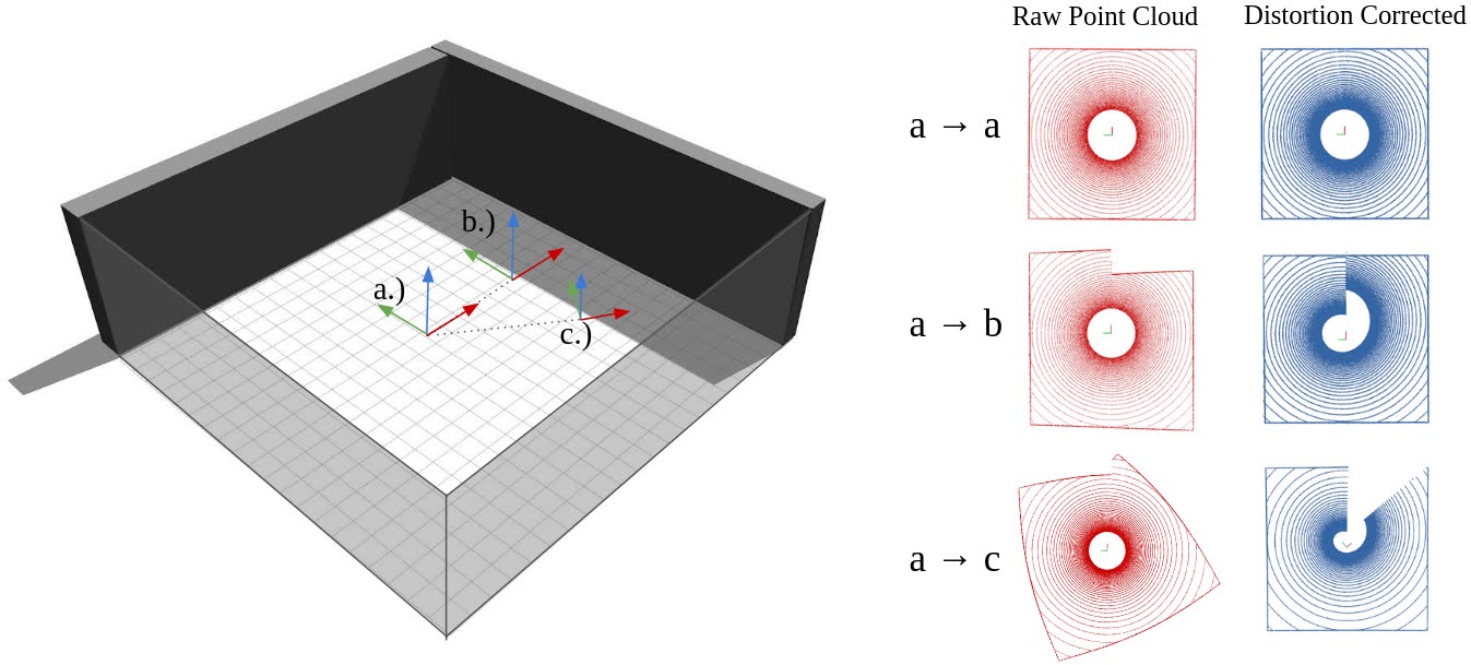
Before describing our solution, it is helpful to develop a better understanding of motion distortion through a simple simulation. Consider a mechanically spinning LIDAR unit placed inside a rectangular room, as illustrated in Fig. 1. A LIDAR image (or scan) is generated each time the LIDAR spins $360^{\circ}$ about the LIDAR’s vertical ($z$) axis. Define the LIDAR scan to begin when the rotating beam aligns with the positive $x$ direction in a coordiante system attached to the LIDAR stator, which we will label the body frame. In the figure, starting and ending locations of the LIDAR are indicated by vector-bases where the spin axis is shown in blue and the scan-initiation axis is shown in red. Now consider three cases, one in which the sensor remains stationary during the scan (starting and ending at the pose labeled a), a second in which the sensor undergoes pure translation (starting at a and ending at b), and a third in which the sensor undergoes both translation and rotation (starting at a and ending at c). Each of the three cases creates a distinct LIDAR point cloud shown, from an aerial view, in a column labeled “Raw Point Cloud” (red). In all cases, a circle appears in the middle of the point cloud, reflecting an elevation cutoff, with the simulated LIDAR unit unable to generate samples below $30^{\circ}$ under the horizon. The point clouds were generated assuming a uniform rate of motion between the start and end points. Importantly, the raw images are distorted (except in the stationary case), such that the walls of the room do not form a perfect square. Accounting for platform motion, however, points can be shifted from body-frame coordinates to world-frame coordinates. Unwarped point clouds are shown in Fig. 1 as a column of images (blue) labeled “Distortion Corrected.” Importantly, these distortion-corrected images all recover the correct room shape, bounded by a square wall. In the last case ($a\rightarrow c$), a wedge of missing data appears because the LIDAR stator rotates clockwise, opposite the counterclockwise rotation of the LIDAR rotor, such that the entire room is not visualized during a single scan.

For map-matching applications, pose is estimated relative to a reference image. For instance, the reference image might be constructed by registering a series of sequential scans from a moving LIDAR, in order to create a mosaic image or high-definition (HD) map. The performance of this registration operation is greatly enhanced if the current scan (captured in the frame of the LIDAR) can be unwarped (converted to the world frame) before registration to the map. In the case of the rectangular room of Fig. (1), the map will look very much like the scan for the static case ($a\rightarrow a$). If a new LIDAR image were generated during translation ($a\rightarrow b$) or combined translation and rotation ($a\rightarrow c$) the resulting raw image (red) will be harder to align with a map of the room than the corresponding distortion-corrected image (blue).

The main focus of this paper is that distortion correction is possible using only the current LIDAR scan and a map. If LIDAR motion is not known, then we can infer the motion by registering the current image to a map while also testing various unwarping transformations, in order to determine the combination of registration and unwarping that results in best alignment. We develop this idea for simultaneous estimation of pose and motion-correction states in subsequent sections.

We intentionally restrict our analysis to cases where the reference image is an undistorted map. In concept, the process of aligning and unwarping images could also be performed on sequential images, for instance to implement LIDAR odometry. If the reference image were distorted, our estimated motion-distortion correction would reflect relative velocity and angular velocity (changes between scans) but not absolute velocity and angular velocity (motion relative to the ground). In other words, our approach does not correct distortion in the reference image.

III Implementation

This section develops a snapshot minimum-squared error (MSE) estimator, which infers both the relative-pose (translation and rotation) and motion-distortion parameters for a current LIDAR scan by comparison to an undistorted reference map. We call the algorithm Velocity-corrected Iterative Compact Ellipsoidal Transformation (VICET).

III-A Algorithm Formulation

To start, we define two relevant reference frames: one associated with the map and a second associated with the LIDAR stator. We characterize the map frame by an origin $Q_{M}$ and a coordinate system defined by the basis $M$. We define the LIDAR stator frame, which we also called the body frame, with a reference point $Q_{B}$ and a body-fixed coordinate system $B$. The body frame translates and rotates relative to the map frame over time, as shown in Fig. 2. Although the LIDAR rotor spins about a fixed axis of B, we do not define a distinct reference frame for the rotor, since the LIDAR system converts measurements to the stator frame B using encoder data.

Figure 2: The frame of the LIDAR stator (or body) B moves relative to the map frame M. For illustration purposes, the bases are shown in 2D, viewed from above. The progress of time is indicated by the shaded gray arrow, with the LIDAR beam recording measurements (red dots) as it sweeps a full circle between time $t=0$ and time $t=T$.

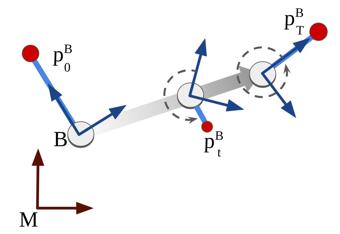
A map matching algorithm seeks to find the rigid transform that aligns the raw LIDAR scan to the map at the beginning of the scan, at time $t=0$. The motion states are inferred to unwarp the LIDAR scan given its motion between the beginning of the scan and the end of the scan, which occurs at $t=T$. Using a zero-order hold model, we approximate that the velocity and angular velocity of $B$ relative to $M$ remains constant for times $t\in[0,T]$. Now consider a LIDAR measurement vector $\mathbf{p}^{B}_{t}$. The vector $\mathbf{p}^{B}_{t}$ describes the position of a feature in the world (or on the map) relative to the body-frame reference point $Q_{B}$ using body-fixed coordinates (specified by the trailing superscript $B$) at a time $t$ (specified by the trailing subscript). The following transformation converts this measurement to $\mathbf{p}^{M}_{t}$, which expresses the same measurement in map coordinates relative to the map origin $Q_{M}$:

$$\mathbf{p}^{M}_{t}={}^{M}\mathbf{R}^{B}_{t}\mathbf{p}^{B}_{t}+\mathbf{m}^{M}_{t}$$ (1)

Here the rotation matrix ${}^{M}\mathbf{R}^{B}_{t}$ converts from the $B$ basis to the $M$ basis at time $t$. The translation $\mathbf{m}^{M}_{t}$ expresses the vector from $Q_{M}$ to $Q_{B}$ at time $t$, in map-fixed coordinates.

As a next step, we decompose the terms in (1) to relate them to initial states and change states. This decomposition is easiest to develop for the translation term $\mathbf{m}^{M}_{t}$, which is linear. Given the zero-order hold assumption, we can rewrite the translation using the lever rule to interpolate between an initial translation $\mathbf{m}^{M}_{0}$ and a final translation $\mathbf{m}^{M}_{T}$. The lever rule can be written

$$\mathbf{m}^{M}_{t}=\mathbf{x}_{0}+s\Delta\mathbf{x}$$ (2)

This formulation introduces the following shorthand notation: $\mathbf{x}_{0}=\mathbf{m}^{M}_{0}$, $\Delta\mathbf{x}=\mathbf{m}^{M}_{T}-\mathbf{m}^{M}_{0}$, and $s=t/T$. The scaled time $s$, derived from the LIDAR time tag for each measurement, is normalized such that $s\in[0,1]$. The variables $\mathbf{x}_{0}$ and $\Delta\mathbf{x}$ are identified specifically because these are states that the estimator will infer.

Just as initial and change states are defined for translation, similar states must be defined for rotation. In our implementation, we use an array of three Euler angles $\mathbf{\Theta_{0}}$ to describe the initial orientation of the body frame. The rotation matrix is constructed as a function $f$ of the Euler angles $\mathbf{\Theta_{0}}$.

$${}^{M}\mathbf{R}^{B}_{0}=f(\mathbf{\Theta_{0}})$$ (3)

The orientation change is described by a set of three angles $\Delta\mathbf{\Theta}$. The final rotation matrix at time $T$ can be related, as follows, to the initial rotation matrix and $\Delta\mathbf{\Theta}$.

$${}^{M}\mathbf{R}^{B}_{T}({}^{M}\mathbf{R}^{B}_{0})^{-1}=f(\mathbf{\Delta\Theta})$$ (4)

Compiling the initial and change states together, we can define a combined state vector $\mathcal{X}\in\mathbb{R}^{12\times 1}$, which we will estimate by comparing the LIDAR scan to a map.

$$\mathcal{X}=\begin{bmatrix}\mathbf{x}_{0}\\ \Delta\mathbf{x}\\ \mathbf{\Theta_{0}}\\ \Delta\mathbf{\Theta}\end{bmatrix}$$ (5)

To relate (1) to the states in (5), we use a Taylor series expansion, in which we expand (1) about a reasonable guess. In implementation, we seed the initial position and Euler angles with a rough guess, and we seed the change parameters with zero values. The affine terms of the Taylor series are:

$$\mathbf{p}^{M}_{t}=({}^{M}\mathbf{\hat{R}}^{B}_{t}+\delta{}^{M}\mathbf{R}^{B}_{t})\mathbf{p}^{B}_{t}+\mathbf{\hat{m}}^{M}_{t}+\delta\mathbf{m}^{M}_{t}.$$ (6)

Here we employ a hat notation to identify terms computed using the initial guess. Also, we introduce a $\delta$ notation to identify linear perturbations.

Because the translation term is linear, the translation perturbation can be obtained from the derivative of (7):

$$\delta\mathbf{m}^{M}_{t}=\delta\mathbf{x}_{0}+s\delta\Delta\mathbf{x}.$$ (7)

The rotation-perturbation $\delta\mathbf{R}$ is obtained from the rotation-matrix derivative, which in the small angle limit is

$$\delta{}^{M}\mathbf{R}^{B}_{t}=[\delta\mathbf{\Theta}{\times}]\;\,{}^{M}\hat{\mathbf{R}}^{B}_{t}.$$ (8)

Here $\delta\mathbf{\Theta}$ is an angular correction converted to a cross-product by the $[\_\_\times]$ operator. This matrix, for a generic vector v with elements $\{v1,v2,v3\}$ is:

$$[\mathbf{v}\times]=\begin{bmatrix}0&-v_{3}&v_{2}\\ v_{3}&0&-v_{1}\\ -v_{2}&v_{1}&0\end{bmatrix}.$$ (9)

Though Euler angles do not sum in general, summation is a good approximation after linearization, and so $\delta\mathbf{\Theta}$ can be written in terms of initial and change states:

$$\delta\mathbf{\Theta}=\delta\mathbf{\Theta}_{0}+s\delta\Delta\mathbf{\Theta}$$ (10)

Substituting (7)-(10) into (6), we obtain a linear system of equations relating the correction states to the LIDAR data:

$$\mathbf{p}^{M}_{t}={}^{M}\mathbf{\hat{R}}^{B}_{t}\mathbf{p}^{B}_{t}+\mathbf{\hat{m}}^{M}_{t}+\mathbf{H}_{\mathcal{X}}\delta\mathcal{X}.$$ (11)

Here the the state-perturbation vector $\delta\mathcal{X}\in\mathbb{R}^{12\times 1}$ is

$$\delta\mathcal{X}=\begin{bmatrix}\delta\mathbf{x}_{0}\\ \delta\Delta\mathbf{x}\\ \delta\mathbf{\Theta_{0}}\\ \delta\Delta\mathbf{\Theta}\end{bmatrix},$$ (12)

and the Jacobian $\mathbf{H}_{\mathcal{X}}\in\mathbb{R}^{3\times 12}$ is

$${\mathbf{H_{\mathcal{X}}}}=\begin{bmatrix}\mathbf{I}&s\mathbf{I}&-\mathbf{P}&-s\mathbf{P}\\ \end{bmatrix},$$ (13)

where the cross-product is embedded in $\mathbf{P}=[{}^{M}\hat{\mathbf{R}}^{B}_{t}\,\mathbf{p}^{B}_{t}\times]$.

In order to invert equation (11) and obtain the state corrections (12), two important details remain. One issue is data association, which is to say that the body-frame point described by $\mathbf{p}^{B}_{t}$ must be matched to the corresponding point $\mathbf{p}^{M}_{t}$ in the map data. A second issue is that (11) contains only 3 equations, so several such systems must be solved simultaneously to enable an independent solution for the twelve states in (12). Moreover, to avoid condition-number deficiencies, points must be compared from a wide range of $s$ values (meaning a wide range of angles through the LIDAR rotational sweep); otherwise if the range of $s$ is narrow, the structure of (7) undermines the independence of $\delta\mathbf{x}_{0}$ and $\delta\Delta\mathbf{x}$, and similarly the structure of (10) undermines the independence of $\delta\mathbf{\Theta}_{0}$ and $\delta\Delta\mathbf{\Theta}$. In the rest of this section, we assume a broad swathe of features are imaged across the full range of $s$, such that a well-condition set of equations can be obtained. Thus, our main focus is data association.

To address the data association problem, we use a voxel-based strategy, as employed by the popular NDT algorithm and our variant ICET. In these algorithms, point clouds are situated within a three-dimensional grid, consisting of volume elements called voxels. If the voxel grid is defined in frame M, it is trivial to assign each LIDAR point from the HD-map to the voxel containing it. Points from the current scan can also be associated with voxels, after the scan is transformed to frame M using the initial guess. An improved registration can then be inferred by aligning the distribution of map points to the distribution of current-scan points within each voxel. Ultimately, the grid enforces spatial associations, thereby avoiding association problems that arise in ICP, LOAM and other methods in the form of ambiguities caused by incorrect matches of points (or extracted features) between the map and the current scan.

To compare distributions of points in a given voxel, we take the expected value of (11) across all points in the voxel, which gives the following.

$$E\big{(}\mathbf{p}^{M}_{t}\big{)}=E\big{(}{}^{M}\mathbf{\hat{R}}^{B}_{t}\mathbf{p}^{B}_{t}\big{)}+E\big{(}\mathbf{\hat{m}}^{M}_{t}\big{)}+E\big{(}\mathbf{H}_{\mathcal{X}}\delta\mathcal{X}\big{)}$$ (14)

On the right side of the equation, the rotation matrix ${}^{M}\mathbf{\hat{R}}^{B}_{t}$, the translation vector $\mathbf{\hat{m}}^{M}_{t}$, and the state-correction vector $\mathcal{X}$ are the same for all points in the cloud (and therefore also for all points in voxel). Accordingly, these three terms can be moved outside the expected-value operator.

$$E\big{(}\mathbf{p}^{M}_{t}\big{)}={}^{M}\mathbf{\hat{R}}^{B}_{t}E\big{(}\mathbf{p}^{B}_{t}\big{)}+\mathbf{\hat{m}}^{M}_{t}+E\big{(}\mathbf{H}_{\mathcal{X}}\big{)}\delta\mathcal{X}$$ (15)

In this equation, the matrix $\mathbf{H}_{\mathcal{X}}$ depends on $s$ and $P$, which have slightly different values for each point in the voxel. Those variations are small in practice, and a very good approximation is obtained by defining ${}^{(j)}\mathbf{\tilde{H}}_{\mathcal{X}}$, which is equivalent to $\mathbf{H}_{\mathcal{X}}$ except that, in (13), the $s$ value is determined for the midpoint of voxel $j$ and $\mathbf{P}$ is set to $\mathbf{P}=[{}^{M}\hat{\mathbf{R}}^{B}_{mid}\;{}^{(j)}\mathbf{\mu}^{B}\;\times]$, with the rotation matrix also evaluated at the voxel midpoint. Using this simplification, we can closely approximate (15) by setting ${}^{(j)}\mathbf{\tilde{H}}_{\mathcal{X}}\approx E\big{(}\mathbf{H}_{\mathcal{X}}\big{)}$. The remaining two expected-value operations are averages across LIDAR points in a given voxel $j$. Accordingly, we invoke the $j$ index and introduce the notation ${}^{(j)}\mathbf{\mu}^{M}=E\big{(}\mathbf{p}^{M}_{t}\big{)}$ and ${}^{(j)}\mathbf{\mu}^{B}=E\big{(}\mathbf{p}^{M}_{t}\big{)}$. The vector ${}^{(j)}\mathbf{\mu}^{M}$ is the mean position for all points from the map that fall in voxel $j$. The vector ${}^{(j)}\mathbf{\mu}^{B}$ is the mean position, in body-frame coordinates, for all current-scan points falling in voxel $j$. Substituting ${}^{(j)}\mathbf{\tilde{H}}_{\mathcal{X}}$, ${}^{(j)}\mathbf{\mu}^{M}$, and ${}^{(j)}\mathbf{\mu}^{B}$ into (15) gives the following equation.

$${}^{(j)}\mathbf{\mu}^{M}={}^{M}\mathbf{\hat{R}}^{B}_{t}\;\;{}^{(j)}\!\mathbf{\mu}^{B}+\mathbf{\hat{m}}^{M}_{t}+{}^{(j)}\mathbf{\tilde{H}}_{\mathcal{X}}\delta\mathcal{X}$$ (16)

The state-correction vector $\delta\mathcal{X}$ is obtained by solving this equation simultaneously over all voxels. With a sufficient number of geometrically diverse voxels, the system is overdetermined, and a weighted least-squares solution can be used to mitigate measurement noise.

$$\delta\mathcal{X}=(\mathbf{H}^{T}\mathbf{W}\mathbf{H})^{-1}\mathbf{H}^{T}\mathbf{W}~{}\mathbf{y}$$ (17)

Here $\mathbf{W}$ is a weighting matrix, $\mathbf{H}$ is the concatenation of the matrices ${}^{(j)}\mathbf{\tilde{H}}_{\mathcal{X}}$ over all voxels $j$, and the $\mathbf{y}$ is the concatenation of the observables ${}^{(j)}\mathbf{y}$ over the same voxels, where

$${}^{(j)}\mathbf{y}={}^{(j)}\mathbf{\mu}^{M}-{}^{M}\mathbf{\hat{R}}^{B}_{t}\;\;{}^{(j)}\!\mathbf{\mu}^{B}-\mathbf{\hat{m}}^{M}_{t}.$$ (18)

The weighting matrix $\mathbf{W}$ is constructed from the measurement-error covariance for $\mathbf{y}$, as discussed in [22]. The same reference also provides numerical tools that allow (17) to be solved using a block decomposition of $\mathbf{H}$, $\mathbf{W}$, and $\mathbf{y}$. The decomposition enhances computational efficiency and reduces memory requirements.

Once the correction states are computed, the initial guess $\hat{\mathcal{X}}$ can be updated using the following equation.

$$\hat{\mathcal{X}}\rightarrow\hat{\mathcal{X}}+\delta\mathcal{X}$$ (19)

Newton iteration can be used to converge on a solution. In practice, we obtained better results using Levenberg-Marquardt optimiztion [23].

III-B Additional Details

In this section we identify practical details related to instantiating the above VICET algorithm in code.

Timestamps: Timestamps of LIDAR points can be approximated by using beam angle $\psi$. It is important not to group points recorded at different times (e.g., at the beginning and end of the scan). We address the aliasing issue by defining a voxel boundary at $0^{\circ}$ (start of scan) and then removing occasional aberational points with $\psi<0^{\circ}$ or $\psi\geq 360^{\circ}$.

Initialization: As mentioned in connection with (6), VICET assumes a reasonable estimate of initial pose. We obtained the initial pose by first running a standard scan-match, specifically NDT; VICET then improves this estimate by compensating for motion distortion.

Extended surfaces: NDT fails to recognize that walls (and other flat surfaces stretching across voxel boundaries) provide useful information only in the surface-normal direction; to enhance convergence reliability and accuracy, we incorporate ICET [4] extended-surface suppression into VICET.

IV Experiment: HD-Map Registration

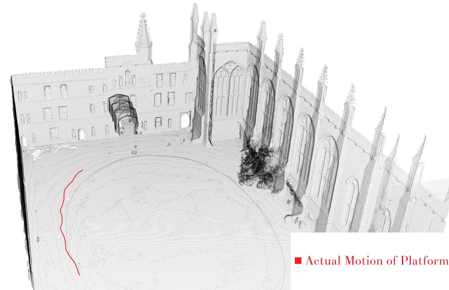
In this section we evaluate the performance of snapshot scan-to-map localization using VICET, and we compare with two other widely used snapshot algorithms: NDT and ICP. For our evaluation, we make use of the Newer College Dataset [24] which contains a rosbag of raw LIDAR data packets and associated ground truth. The dataset also includes a survey-grade HD map of the structured environment recorded on a separate Leica total station. Specifically, we utilize 200 consecutive LIDAR scans of Newer College Data from the Quad With Dynamics trajectory, where a researcher runs while swinging the LIDAR sensor at head height, to approximate the dynamics of a multi-rotor drone [24]. The ground-truth position for the 200 scans is shown in Fig. (3), superposed on the HD map.

Figure 3: Ground truth for each of 200 scans, superimposed on the HD Map

Snapshot processing was conducted by matching each individual scan to the map, without reference to any other scan from the sequence. Snapshot position and orientation estimates were obtained via three distinct methods: VICET, ICP, and NDT. Note that VICET was initialized with NDT, and so the same spherical voxel grid [25] was used for both VICET and NDT in order to ensure a controlled comparison. The three methods were compared using absolute-error and chamfer-distance performance metrics.

Figure 4: Translation error (top) and yaw error (bottom) when registering 200 raw LIDAR scans against a static HD Map.

IV-A Absolute-Error Results

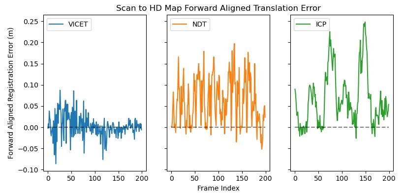
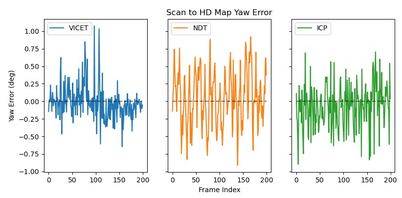
An absolute-error vector was formed from each estimate by subtracting ground-truth values, which were referenced to LIDAR position and orientation at the start of the scan. We display error values in Fig. (4). Specifically the figure shows forward-translation error (top) and yaw-angular error (bottom) for each of the three algorithms under comparison. Forward error was typically the largest component of the translation-error vector. By contrast with translation errors, angular errors did not exhibit directional dependence, so we selected as representative the angular-error component in the yaw sense (about the map-fixed vertical axis).

Absent motion-distortion correction, the forward-errors for NDT and ICP exhibit a significant bias. As evident in Fig. (4), errors for both NDT (orange) and ICP (green) are generally above zero, with very few negative values. By comparison, the corresponding VICET forward-error values (blue) appear to be zero-centered. Additionally, the distribution of the VICET forward-error values is narrower than the distributions for NDT (orange) or ICP (green). These trends were quantified by computing the mean and standard deviation of the forward-error values across each of the 200 samples, statistics that are reported in Table (I). The table confirms the statistical mean of forward error for VICET is an order of magnitude smaller than for uncompensated ICP or NDT (0.269 cm as compared to more than 6.0 cm); similarly, the standard deviation of forward error for VICET is better than half that for ICP or NDT (2.6 cm as compared to more than 5.4 cm).

Similar trends are observed in yaw, with motion-corrected VICET outperforming the uncorrected NDT and ICP algorithms. Again, VICET exhibits a substantially smaller bias ($0.015^{\circ}$ compared to $0.05^{\circ}$ or more) and a slightly narrower standard deviation ($0.24^{\circ}$ as compared to $0.31^{\circ}$ or more).

TABLE I: Localization Error

	Forward Translation Error		Yaw Error
	Mean (cm)	STD (cm)	Mean (deg)	STD (deg)
ICP	6.671	6.435	-0.0657	0.310
NDT	6.005	5.432	0.0509	0.386
VICET	0.269	2.612	-0.015	0.242

TABLE II: Normalized Chamfer Distance ($\text{cm}^{2}$)

	Quad With Dynamics	Dynamic Spinning
ICP	0.869	3.317
NDT	0.814	3.045
VICET	0.732	2.118

IV-B Chamfer Distance

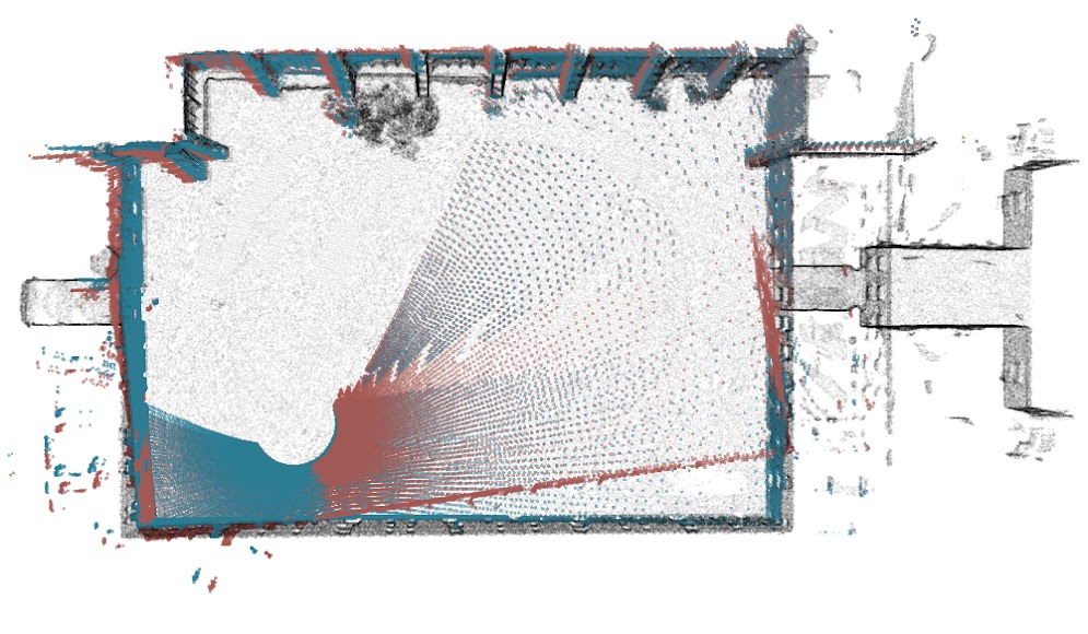
We used a second metric, chamfer distance, to directly compare the shape of the map to that of the current scan (after registration). Chamfer distance is defined as the sum of the squared distances for all nearest-point correspondences between two clouds. This metric effectively compares the different shapes of registered scans visualized in Fig. (5), as referenced to the map. A larger shape difference corresponds to a larger chamfer distance. Notably, the chamfer distance metric does not rely on ground truth.

Some minimal data cleaning was required to compare chamfer distance in a meaningful way. As a first step, ICP, NDT and VICET were used to register a scan to the map. A chamfer distance was then computed applying an outlier rejection criterion (no points considered outside the inflated convex hull for the map, with 5% applied in our analysis). The process was repeated for all 200 scans considered from the Quad with Dynamics trajectory. Each chamfer distance was then normalized by the number of points in the associated LIDAR cloud, to account for scan-to-scan variability in the number of non-return points. Normalized chamfer distances were then averaged across all 200 cases. The results are compiled in Table (II).

The table (column labeled Quad with Dynamics) shows that the average normalized chamfer distance for VICET was slightly better than for either NDT or ICP (0.73 cm² as compared to 0.81 cm² or more). This result indicates that the output from VICET is indeed a better approximations of the map than the outputs of either NDT or ICP.

Because these chamfer distances were only modestly separated, we evaluated a second Newer College trajectory, labeled Dynamic Spining, to verify the dependence of chamfer distance on distortion severity. The second trajectory contained more motion distortion than the first. Normalized chamfer-distance results were computed and the data compiled, as recorded in the table (column labeled Dynamic Spinning). As expected, the chamfer distances were higher for this case than for the prior case (Quad with Dynamics). Moreover, the chamfer distance metric for VICET was again better than for either NDT or ICP (2.1 cm² as compared to 3.0 cm² or more).

Figure 5: Registered point clouds with and without motion-distortion compensation. As compared to the NDT-registered data (red), the VICET corrected data (blue) more closely resemble the HD-Map (black).

V Discussion and Future Work

The experimental results from the prior section strongly support the importance of motion-distortion correction for high-accuracy scan-to-map matching. Distortion not only introduces systematic biases but also inflates the standard deviation, implying that uncertainty quantification methods (e.g., estimators predicting state-error covariance) will perform poorly without distortion-mitigation. The higher standard deviation (and wider error distribution) for uncompensated algorithms may possibly be explained by the registration-process “hunting” over the space of poses observed between the start and end of the scan ($0\leq t\leq T$); those intermediate poses are all partially represented in the raw scan.

In this work, our primary emphasis is on achieving high-accuracy scan-to-map matching with a reasonable initial guess. VICET, by itself, does not solve the Kidnapped Robot problem [26], however, VICET could be layered with other algorithms that solve the global search problem, enhancing their accuracy. In the simplest form, VICET might be run to convergence from a number of initial guesses using an exhaustive search, a particle filter, or through a pose-invariant “global” registration network such as DeepGMR [27] before compensating for distortion with VICET.

Though not developed for LIDAR odometry (LO), VICET might still have possible future LO applications. VICET provides immediate unwarping when comparing a new scan to an LO submap, without delay. By comparison, many existing LO algorithms infer unwarping in one scan by estimating the distance traveled from that scan to the next, a process which inherently adds a delay (typically 50-200 ms to capture the next scan). Such delays are undesirable for feedback-control loops, as pure delays cause sluggish performance and erode stability margins.

To apply VICET in larger, more complex, and occluded environments, it may be necessary to address sensitivity to perspective shift bias [28]. Perspective bias can occur in HD-Map matching when LIDAR points exist in the map but are not visible from the location of the current scan, because they are occluded by foreground surfaces. New methods are needed to condition voxel-based processing to minimize systematic errors due to perspective effects. Fortunately, in the Newer College Dataset, the walls of the courtyard are mostly visible from all vantage points, so perspective errors did not play a major role in this analysis.

VI Conclusion

In this paper we introduced VICET, a novel algorithm to solve the scan-to-map matching problem for a single LIDAR point cloud. VICET soves for twelve states, six describing a rigid transform aligning the scan to the map, and six more to account for distortion due to platform motion during the creation of the cloud. In contrast with other motion-distortion methods, our approach requires only a single LIDAR scan and no external sensor data.

Through experiments on real-world data, we demonstrate VICET improves accuracy over conventional NDT and ICP, reducing the translation-bias for map matching (by an order of magnitude, from 6.9 cm to 0.27 cm) while reducing one-sigma variations (from 5.4 cm to 2.6 cm). VICET also reduced bias and variance for orientation estimation. These enhancements are relevant for precision automotive and urban air mobility applications.

References

- [1] Paul J Besl and Neil D McKay “Method for registration of 3-D shapes” In Sensor fusion IV: control paradigms and data structures 1611, 1992, pp. 586–606 Spie
- [2] Peter Biber and Wolfgang Straßer “The normal distributions transform: A new approach to laser scan matching” In Proceedings 2003 IEEE/RSJ International Conference on Intelligent Robots and Systems (IROS 2003)(Cat. No. 03CH37453) 3, 2003, pp. 2743–2748 IEEE
- [3] Kenji Koide, Masashi Yokozuka, Shuji Oishi and Atsuhiko Banno “Globally consistent 3D LiDAR mapping with GPU-accelerated GICP matching cost factors” In IEEE Robotics and Automation Letters 6.4 IEEE, 2021, pp. 8591–8598
- [4] Matthew McDermott and Jason Rife “ICET Online Accuracy Characterization for Geometry-Based Laser Scan Matching” In arXiv preprint arXiv:2306.08690, 2023
- [5] Xiaohu Lin, Fuhong Wang, Bisheng Yang and Wanwei Zhang “Autonomous vehicle localization with prior visual point cloud map constraints in GNSS-challenged environments” In Remote Sensing 13.3 MDPI, 2021, pp. 506
- [6] Todor Stoyanov, Martin Magnusson, Henrik Andreasson and Achim J Lilienthal “Fast and accurate scan registration through minimization of the distance between compact 3D NDT representations” In The International Journal of Robotics Research 31.12 Sage Publications Sage UK: London, England, 2012, pp. 1377–1393
- [7] Ji Zhang and Sanjiv Singh “LOAM: Lidar odometry and mapping in real-time.” In Robotics: Science and Systems 2.9, 2014, pp. 1–9 Berkeley, CA
- [8] Andrea De Maio and Simon Lacroix “Deep bayesian icp covariance estimation” In 2022 International Conference on Robotics and Automation (ICRA), 2022, pp. 6519–6525 IEEE
- [9] Qing Li et al. “Lo-net: Deep real-time lidar odometry” In Proceedings of the IEEE/CVF Conference on Computer Vision and Pattern Recognition, 2019, pp. 8473–8482
- [10] Younggun Cho, Giseop Kim and Ayoung Kim “Unsupervised geometry-aware deep lidar odometry” In 2020 IEEE international conference on robotics and automation (ICRA), 2020, pp. 2145–2152 IEEE
- [11] Gaurav Pandey, James R McBride and Ryan M Eustice “Ford campus vision and lidar data set” In The International Journal of Robotics Research 30.13 SAGE Publications Sage UK: London, England, 2011, pp. 1543–1552
- [12] Jean–Luc Déziel et al. “Pixset: An opportunity for 3D computer vision to go beyond point clouds with a full-waveform LiDAR dataset” In 2021 IEEE International Intelligent Transportation Systems Conference (ITSC), 2021, pp. 2987–2993 IEEE
- [13] Holger Caesar et al. “nuscenes: A multimodal dataset for autonomous driving” In Proceedings of the IEEE/CVF conference on computer vision and pattern recognition, 2020, pp. 11621–11631
- [14] Pratap Misra “Global positioning system: Signal, measurement, and performance; revised 2nd edition” Ganga-Jamuna Press, 2010
- [15] Peng Xie and Mark G Petovello “Measuring GNSS multipath distributions in urban canyon environments” In IEEE Transactions on Instrumentation and Measurement 64.2 IEEE, 2014, pp. 366–377
- [16] Kimiaki Inui, Masahide Morikawa, Masafumi Hashimoto and Kazuhiko Takahashi “Distortion Correction of Laser Scan Data from In-vehicle Laser Scanner based on Kalman Filter and NDT Scan Matching.” In ICINCO (2), 2017, pp. 329–334
- [17] G.. Franklin, J.. Powell and A. Emami-Naeini “Feedback control of dynamic systems” Pearson, 2015
- [18] Timothy P. Setterfield, Robert A. Hewitt, Antonio Terán Espinoza and Po-Ting Chen “Feature-Based Scanning LiDAR-Inertial Odometry Using Factor Graph Optimization” In IEEE Robotics and Automation Letters 8.6, 2023, pp. 3374–3381 DOI: 10.1109/LRA.2023.3266701
- [19] Shinsuke Shimojo, Gerald H Silverman and Ken Nakayama “Occlusion and the solution to the aperture problem for motion” In Vision research 29.5 Elsevier, 1989, pp. 619–626
- [20] Seungpyo Hong, Heedong Ko and Jinwook Kim “VICP: Velocity updating iterative closest point algorithm” In 2010 IEEE International Conference on Robotics and Automation, 2010, pp. 1893–1898 IEEE
- [21] Olivier N Kigotho, Jason H Rife and Hadi Wassaf “Lane-Keeping Safety and Time Correlation of Navigation Errors” In Proceedings of the 2022 International Technical Meeting of The Institute of Navigation, 2022, pp. 1329–1342
- [22] Matthew McDermott and Jason Rife “Enhanced laser-scan matching with online error estimation for highway and tunnel driving” In Proceedings of the 2022 International Technical Meeting of The Institute of Navigation, 2022, pp. 643–654
- [23] Henri P Gavin “The Levenberg-Marquardt algorithm for nonlinear least squares curve-fitting problems” In Department of civil and environmental engineering, Duke University 19, 2019
- [24] Milad Ramezani et al. “The newer college dataset: Handheld lidar, inertial and vision with ground truth” In 2020 IEEE/RSJ International Conference on Intelligent Robots and Systems (IROS), 2020, pp. 4353–4360 IEEE
- [25] Matthew McDermott and Jason Rife “Mitigating Shadows in LIDAR Scan Matching Using Spherical Voxels” In IEEE Robotics and Automation Letters 7.4, 2022, pp. 12363–12370 DOI: 10.1109/LRA.2022.3216987
- [26] Sebastian Thrun “Probabilistic robotics” In Communications of the ACM 45.3 ACM New York, NY, USA, 2002, pp. 52–57
- [27] Wentao Yuan et al. “Deepgmr: Learning latent gaussian mixture models for registration” In Computer Vision–ECCV 2020: 16th European Conference, Glasgow, UK, August 23–28, 2020, Proceedings, Part V 16, 2020, pp. 733–750 Springer
- [28] Jason H Rife and Matthew McDermott “Characterizing Perspective Error in Voxel-Based LIDAR Scan Matching” In Proceedings of the 2023 International Technical Meeting of The Institute of Navigation, 2023, pp. 1043–1057