Pretty darn good control: when are approximate solutions better than approximate models

Abstract

Existing methods for optimal control struggle to deal with the complexity commonly encountered in real-world systems, including dimensionality, process error, model bias and data heterogeneity. Instead of tackling these system complexities directly, researchers have typically sought to simplify models to fit optimal control methods. But when is the optimal solution to an approximate, stylized model better than an approximate solution to a more accurate model? While this question has largely gone unanswered owing to the difficulty of finding even approximate solutions for complex models, recent algorithmic and computational advances in deep reinforcement learning (DRL) might finally allow us to address these questions. DRL methods have to date been applied primarily in the context of games or robotic mechanics, which operate under precisely known rules. Here, we demonstrate the ability for DRL algorithms using deep neural networks to successfully approximate solutions (the “policy function” or control rule) in a non-linear three-variable model for a fishery without knowing or ever attempting to infer a model for the process itself. We find that the reinforcement learning agent discovers a policy that outperforms both constant escapement and constant mortality policies—the standard family of policies considered in fishery management. This DRL policy has the shape of a constant escapement policy whose escapement values depend on the stock sizes of other species in the model.

Keywords Optimal Control  $\cdot$ Reinforcement Learning  $\cdot$ Uncertainty  $\cdot$ Decision Theory

1 Introduction

Much effort has been spent grappling with the complexity of our natural world in contrast to the relative simplicity of the models we use to understand it. Heroic amounts of data and computation are being brought to bear on developing better, more realistic models of our environments and ecosystems, in hopes of improving our capacity to address the many planetary crises. But despite these efforts and advances, we remain faced with the difficult task of figuring out how best to respond to these crises. While simplified process models for the population dynamics have historically allowed for exploration of large decision spaces, the new wave of rich models are applied to highly oversimplified descriptions of potential actions they seek to inform. For instance, Global Circulation Models (GCMs) such as HadCM3 (Pope et al. 2000; C. Gordon et al. 2000; Collins, Tett, and Cooper 2001) model earth’s climate using 1.5M variables, while the comparably vast potential action space is modeled much more minimalistically, with 5 SSP socioeconomic storylines and 7 SSP-RCP marker scenarios summarizing the action space at the IPCC (Riahi et al. 2017).

Even as our research community develops simulations of the natural world that fit only in supercomputers, we analyze a space of policies that would fit on index cards. Similar combinations of rich process models and highly simplified decision models (often not even given the status of ‘model’) are common. Modeling the potential action space as one of a handful of discrete scenarios is sometimes a well justified acknowledgement of the constraints faced by real-world decision-makers – particularly in the context of multilateral decisions – and may seem to reflect a division of responsibilities between ‘scientists’ modeling the ‘natural processes’ and policy-makers who make the decisions. But, more often, this simplification of decision choices is simply mathematically or conceptually convenient. This simplification reflects trade-offs between tractablity and complexity at the basis of any mathematical modeling – if we make both the state space and action space too realistic, the problem of finding the best sequence of actions quickly becomes intractable. However, emerging data-driven methods from machine learning offer a new choice – algorithms that can find good strategies in previously intractable problems, but at the cost of opacity.

In this paper, we focus on a well-developed application of model-based management of the natural world that has long illustrated the trade-offs between model complexity and policy complexity: the management of marine fisheries. Fisheries management is both an important issue to society as well as a rich and frequent test-bed of ecological management more generally. Fisheries are an essential natural resource that provide the primary source of protein for one in every four humans, and have faced widely documented declines due to over-fishing Costello et al. (2016). Fisheries management centers around the process of sampling populations to determine fishing quotas based on population estimates. This decision is often guided by a model of the dynamics of the system. Our paper focuses on the decision side of this problem rather than the measurement step.

Fisheries management has roots in both the fields of ecosystem management and natural resource economics. Both fields might trace their origins to the notion of maximum sustainable yield (MSY), introduced independently by a fisheries ecologist (Schaefer 1954) and the economist (H. S. Gordon and Press 1954) in the same year. From this shared origin, each field would depart from the simplifying assumptions of the Gordon-Schaefer model in divergent ways, leading to different techniques for deriving policies from models.The heart of the management problem is easily understood: a manager seeks to set quotas on fishing that will ensure the long-term profitability and sustainability of the industry. Mathematical approaches developed over the past century may be roughly divided between these two fields: (A) ecologists, focused on ever more realistic models of the biological processes of growth and recruitment of fish while considering a relatively stylized suite of potential management strategies, and (B) economists, focused on far more stylized models of the ecology while exploring a far less constrained set of possible policies. The economist’s approach can be characterized by the mathematics of a Markov decision process (MDP Colin W. Clark 1973; Colin W. Clark 1990; Marescot et al. 2013), in which the decision-maker must observe the stock each year and recommend a possible action. In this approach, the policy space that must be searched is exponentially large – for a management horizon of T decisions and a space of N actions, the number of possible policies is $N^{T}$. In contrast, fisheries ecologists and ecosystem management typically search a space of policies that does not scale with the time horizon. Under methods such as “Management Strategy Evaluation” (MSE, (Punt et al. 2016)) a manager identifies a candidate set of “strategies” a priori, and then compares the performance of each strategy over a suite of simulations to determine which strategy gives the best outcome (i.e. best expected utility). This approach is far more amenable to complex simulations of fisheries dynamics and more closely corresponds to how most marine fishing quotas are managed today in the United States (see stock assessments documented in RAM Legacy Stock Assessment Database 2020).

Recent advances in machine learning may allow us to once again bridge these approaches, while also bringing new challenges of their own. Novel data-driven methods have allowed these models to evolve into ever more complex and realistic simulations used in fisheries management, where models with over 100 parameters are not uncommon (RAM Legacy Stock Assessment Database 2020). Constrained by computational limits, MDP approaches have been intractable on suitably realistic models and largely confined to more academic applications (Costello et al. 2016). However, advances in Deep Reinforcement Learning, (DRL) a sub-field of machine learning, have recently demonstrated remarkable performance in a range of such MDP problems, from video games (Bellemare et al. 2013; Mnih et al. 2013) to fusion reactions (Degrave et al. 2022; Seo et al. 2022) to the remarkable dialog abilities of ChatGPT (OpenAI 2022). RL methods also bring many challenges of their own: being notoriously difficult to train and evaluate, requiring immense computational costs, and presenting frequent challenges with reproducibility. A review of all these issues is beyond our scope but can be found elsewhere (Lapeyrolerie et al. 2022; Chapman et al. 2023). Here, though, we will focus on the issue of opacity and interpretability raised by these methods. In contrast with optimization algorithms currently used in either ecosystem management or resource economics, RL algorithms have no guarantees of or metrics for convergence to an optimal solution. In general, one can only assess the performance of these black box methods relative to alternatives.

In most US fisheries, the mortality policy is often piecewise linear (often with one constant and one linear piece), and the allowable biological catch (ABC) or total allowable catch (TAC) is set at some heuristic (e.g. 80%) below the ‘overfishing limit’, $F_{MSY}$, i.e. the highest (constant) mortality that can be sustained indefinitely (in the model – reality of course does not permit such definitions). This fixed mortality management can be seen, for instance, in most of the fisheries listed in the widely used R.A. Myers Legacy Stock Assessment Database. Here, we have focused on purely constant mortality policies, rather than piecewise linear mortality funcitons, for simplicity. Escapement-based management is less common, except in salmonoids, as it requires closing a fishery whenever the measured biomass falls below $B_{MSY}$.

In this article, we compare against two common methods: constant mortality (CMort) and constant escapement (CEsc), introduced in Text Box 1.

We consider the problem of devising harvest strategies in a for a series of ecosystem models with increasing complexity (Table 1): 1) one species, one fishery: a simple single-species recruitment model based on (May 1977); 2) three species, one fishery: a three-species generalization of model 1), where one of the species is harvested; 3) three species, two fisheries: the same three-species model as above but with two harvested species; 4) three species, two fisheries, parameter variation: a three-species model of which two are harvested, as above, with a time-varying parameter. This last model is meant to be a toy model of climate change’s effect on the system. Across all of these scenarios, two goals are balanced in the decision process: maximizing long-term catch and preventing stock sizes to fall below some a-priori threshold.

Model name	Model eqs.	N. Sp.	Harv. Sp.	Stationary?
Model 1	(3)	1	$X$	Yes
Model 2	(4)	3	$X$	Yes
Model 3	(4)	3	$X$ and $Y$	Yes
Model 4	(4)	3	$X$ and $Y$	No

Table 1: Table of models considered in this paper. Here, N. Sp. is the number of species in the model, Harv. Sp. is the species of the model which are harvested, and Stationary? refers to whether the parameters of the model have fixed values (or, on the contrary, if they vary in time). The only non-stationary case presented in the paper is where $r_{X}$ drifts linearly with time. In the code repository associated to the paper, we consider other possible choices of non-stationarity.

This way, we evaluate classical management strategies (CMort and CEsc) and DRL-based strategies on four different models. This experimental design is summrized in Fig. 1.

Figure 1: An experimental-design type of visualization of the management scenarios considered in this paper. On the x-axis are four different fishery management problems (Table 1). We represent the Model 4’s non-stationarity with a clock next to the X variable, and we intend to use it as an example of a possible simplified model for the effects of climate change. On the y-axis we have different management strategies with which one may control each of the models. On the bottom we have the constant escapement strategy (CEsc), based on calling off all fishing below a certain threshold population value. Above that is the constant mortality strategy (CMort), where one optimizes over constant fishing effort strategies. Finally, on top we have DRL-based strategies where policies are in general functions of the full state of the system, and they are parametrized by a neural network. The specific DRL-based strategy is referred to as PPO+GP in the main text, due to the algorithm used to produce the policy. The results plotted are the average reward obtained by the strategy over 100 episodes, and the fraction of those episodes which do not end with a near-extinction event (denoted Perc for Percentage). We have normalized to the highest reward in each column in order to enhance the comparison between strategies. For illustrative purposes we have color-coded the results using a two-dimensional color legend displayed on the bottom left.

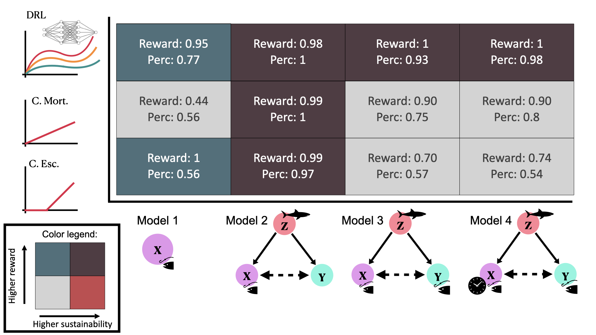
Regarding control for these 4 models, we show the following. Model 1: DRL-based strategies recover the optimal constant escapement (CEsc) policy function. Constant mortality (CMort) performs considerably worse than these three. Model 2: Here, all management strategies perform similarly. Model 3: For this model, DRL outperforms both classical strategies, with CMort surprisingly performing significantly better than CEsc. In particular, we observe that DRL strategies are more sensitive to stochastic variations of the system which allows it to adaptively manage the system to prevent population collapses below the threshold. Model 4: Here, the performance gap between DRL and both classical strategies is maintained.

We show that in the most complex scenario, Model 4, CMort is faced with a tradeoff—the optimal mortality rate leads a rather large fraction of episodes ending with a population crash, whose negative reward is counteracted with a higher economic output. Conversely, more conservative, lower, mortality rates lead to lower total reward on average. The DRL approach side-steps this trade-off by optimizing over a more complex family of possible policies—–policies parametrized by a neural network, as opposed to policies labeled by a single parameter (the mortality rate).

Our findings paint a picture of how a single-species optimal management strategy may lose performance rather dramatically when controlling a more complex ecosystem. Here, DRL performs better from both economical and conservation points of view. Moreover, rather unintuitively, CMort – known to be suboptimal and unsustainable for single-species models – can turn out to even outperform the CEsc – the single-species optimal strategy – for complex ecosystems. Finally, within this regime of complex, possibly varying, ecosystems, we show that DRL consistently finds a policy which effectively either matches the best classical strategy, or outperforms it. We strengthen this result with a stability investigation: we show that random perturbations in the model’s parameter values used do not significantly vary the conclusion that DRL outperforms CEsc.

2 Mathematical models of fisheries considered

Here we mathematically introduce the four fishery models for which we compare different management strategies. In general, the class of models that appear in this context are stochastic, first order, finite difference equations. For $n$ species, these models have the general form

$$\begin{split}\Delta X_{t}&=f_{X}(N_{t})+\eta_{X,t}-M_{X}X_{t}\\ \Delta Y_{t}&=f_{Y}(N_{t})+\eta_{Y,t}-M_{Y}Y_{t}\\ \Delta Z_{t}&=f_{Z}(N_{t})+\eta_{Z,t}-M_{Z}Z_{t}\\ &\dots\end{split}$$ (1)

where $N_{t}=(X_{t},\ Y_{t},\ Z_{t},\ \dots)\in\mathbb{R}^{n}_{+}$ is a vector of populations, $\Delta X_{t}:=X_{t+1}-X_{t}$, $f_{i}:\mathbb{R}^{n}\to\mathbb{R}$ are arbitrary functions, and where $\eta_{i,t}$ are Gaussian random variables. Here, $M_{i}=M_{i}(N_{t})\in\mathbb{R}_{+}$ is a state-dependent fish mortality arising from harvesting the $i$-th species (sometimes this is referred to as fishing effort).

The term $M_{X}X_{t}$ is the total $X$ harvest at time $t$. This formulation of stock recruitment as a discrete finite difference process is common among fisheries, as opposed to continuous time formulations which involve instantaneous growth rates. This growth rate simplifies e.g. the possibly seasonal nature of reproduction (which would need to be accounted for in a realistic continuous-time model) by simply considering the total recruitment experienced by the population over a full year.

The fishing efforts are the control variables of our problem—these may be set by the manager at each time-step to specified values. We make two further simplifying assumptions on the control problem: 1. Full observation: the manager is able to accurately measure $N_{t}$ and use that measurement to inform their decision. 2. Perfect execution: the action chosen by the manager is implemented perfectly (i.e., there is no noise affecting the actual value of the fishing efforts).

Model 1 is a single-species classical model of ecological tipping points. Models 2-4 are all three-species models with similar dynamics. Following this logic, the first subsection will be dedicated to the single-species model and the second will focus on the three-species models.

2.1 The single species model

Optimal control policies for fisheries are frequently based on 1-dimensional models, $n=1$, as described in $Text$ $Box$ $1$. The most familiar model of $f(X)$ is that of logistic growth, for which

$$f(X_{t})=rX_{t}\big{(}1-X_{t}/K\big{)}=:L(X_{t};\ r,K).$$ (2)

Real world ecological systems are obviously far more complicated than this simple model suggests. One particularly important aspect that has garnered much attention is the potential for the kind of highly non-linear functions that can support dynamics such as alternative stable states and hysteresis. A seminal example of such dynamics was introduced in (May 1977), using a one-dimensional model of a prey (resource) species under the pressure of a (fixed) predator. In the notation of eq. (1),

$$f_{X}(X_{t})=L(X_{t};\ r,K)-\frac{\beta HX_{t}^{2}}{c^{2}+X_{t}^{2}}.$$ (3)

In the following, we will denote

$$F(X_{t},H;\ \beta,c):=\frac{\beta HX_{t}^{2}}{c^{2}+X_{t}^{2}}.$$

The model has six parameters: the growth rate $r$ and carrying capacity $K$ for $X$, a constant population $H$ of a species which preys on $X$, the maximal predation rate $\beta$, the predation rate half-maximum biomass $c$, and the variance $\sigma_{X}^{2}$ of the stochastic term $\eta_{X,t}$. (Here and in the following we will center all random variables at zero.)

Eq. (3) is an interesting study case of a tipping point (saddle-node bifurcation) (see Fig. 2). Holding the value of $\beta$ fixed, for intermediate values of $H$ there exist two stable fixed points for the state $X_{t}$ of the system, these two attractors separated by an unstable fixed point. At a certain threshold value of $H$, however, the top stable fixed point collides with the unstable fixed point and both are annihilated. For this value of $H$, and for higher values, only the lower fixed point remains. This also creates the phenomenon of hysteresis, where returning $H$ to its original value is not sufficient to restore $X_{t}$ to the original stable state.

Figure 2: The fixed point diagram for the unharvested dynamics of Model 1 as a function of varying the parameter $\beta H$, assuming zero noise. Stable fixed points (also known as attractors) are plotted using a solid line, while the unstable fixed point is shown as a dotted line.

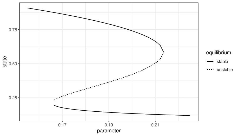
This structure implies two things. First, that a drift in $H$ could lead to catastrophic consequences, with the population $X_{t}$ plummeting to the lower fixed stable point. Second, that if the evolution of $X_{t}$ is stochastic, then, even at values of $H$ below the threshold point, the system runs a sizeable danger of tipping over towards the lower stable point.

2.2 The three species models

Models 2-4 are three-species models and they are all closely related—in fact, their natural dynamics (i.e. dynamics under zero harvest) is essentially given by the same equations:

$$\begin{split}f_{X}(N_{t})&=L(X_{t};\ r_{X},K_{X})-F(X_{t},Z_{t};\ \beta,c)-c_{XY}X_{t}Y_{t},\\ f_{Y}(N_{t})&=L(Y_{t};\ r_{Y},K_{Y})-DF(Y_{t},Z_{t};\ \beta,c)-c_{XY}X_{t}Y_{t},\\ f_{Z}(N_{t})&=\left(b(X_{t}+DY_{t}\right)-d_{Z})Z_{t}.\end{split}$$ (4)

The three species modeled are $X$, $Y$ and $Z$. Species $Z$ preys on both $X$ and $Y$, while the latter two compete for resources. There are thirteen parameters in this model: The growth rate and carrying capacity, $r_{X}$, $K_{X}$, $r_{Y}$ and $K_{Y}$, of $X$ and $Y$. A parameter $c_{XY}$ mediating a Lotka-Volterra competition between $X$ and $Y$. A maximum predation rate $\beta$ and a predation rate half-maximum biomass $c$ specifying how $Z$ forages on $X$ and $Y$. A parameter $D$ regulating a relative preference of $Z$ to prey on $Y$. A death rate $d_{Z}$ and a parameter $b$ scaling the birth rate of $Z$. Finally, the noise variances $\sigma_{X}$, $\sigma_{Y}$ and $\sigma_{Z}$.

The three models will branch off of eq. (4) in the following way. Model 2: here, only $X$ is harvested, that is, in the notation of eq. (1), we fix $M_{Y}=M_{Z}=0$ and leave $M_{X}$ as a control variable. All parameters here are constant. Model 3: as Model 1, but with $X$ and $Y$ being harvested. In other words, we set $M_{Z}=0$ and leave $M_{X}$ and $M_{Y}$ as control variables. Model 4: here $X$ and $Y$ are harvested, but now we include a non-stationary parameter:

$$r_{X}=r_{X}(t)=\begin{cases}1-t/200,\quad&t\leq 100,\\ 1/2,\quad&t>100.\end{cases}$$ (5)

All other parameters are constant. Eq. (5) is intended to reflect in a simple manner a possible effect of climate change: where the reproductive rate of $X$ is reduced linearly over time until it stabilizes.

3 Reinforcement learning

Reinforcement learning (RL) is a way of approaching sequential decision problems through machine learning. All applications of RL can be conceptually separated into two parts: an agent and an environment which the agent interacts with. That is, the agent performs actions within the environment.

After the agent takes an action, the environment will transition to a new state and return a numerical reward to the agent. (See Fig. 1 in (Lapeyrolerie et al. 2022) for a conceptual description of reinforcement learning algorithms.) The rewards encode the agent’s goal. The main task of any RL algorithm is then to maximize the cumulative reward received. This objective is achieved by aggregating experience in what is called the training period and learning from such experience.

The environment is commonly a computer simulation. It is important to note here the role that real time-series data of stock sizes can play in this process. This data is not used directly to train the RL agent, but rather to estimate the model defining the environment. This environment is subsequently used to train the agent. In this paper, we focus on the second step—we take the estimated model of reality as a given, and train an RL agent on it.

Specifically, we consider four environments corresponding to each of the models considered (Table 1). At each time step, the agent observes the state $S$ and enacts some harvest—reducing $X_{t}$ to $X_{t}-M_{X}(N_{t})\cdot X_{t}$, and, for Models 3 and 4, also reducing $Y_{t}$ to $Y_{t}-M_{Y}(N_{t})\cdot Y_{t}$. Here the fish mortality-rates-from-harvest (i.e. $M_{X}=M_{X}(N_{t})$ and $M_{Y}=M_{Y}(N_{t})$), are the agent’s action at time $t$. This secures a reward of $M_{X}(N_{t})X$ for Models 1 and 2, and, similarly, a reward of $M_{X}(N_{t})X+M_{Y}(N_{t})Y$ for Models 3 and 4. After this harvest portion of the time step, the environment evolves naturally according to eqs. (3) and (4) (Sec. 2).

As mentioned previously, discretising time allows a simplification of the possibly seasonal mating behavioral patterns of the species involved. This approximation is commonly used in fisheries for species with annual reproductive cycles (see e.g. (Mangel 2006), Chap. 6). Moreover, the separation of each time-step into a harvest period and a natural growth period assumes that harvest has little disruption on the reproductive process. A detailed model which includes such a disruption is outside of the scope of this work.

3.1 Mathematical framework for RL

The RL environment can be formally described as a discrete time partially observable Markov decision process (POMDP). This formalization is rather flexible and allows one, e.g., to account for situations where the agent may not fully observe the environment state, or where the only observations available to the agent are certain functions of the underlying state. For the sake of clarity, we will only present here the subclass of POMDPs which are relevant to our work: fully observable MDPs (henceforth MDPs for short). An MDP may be defined by the following data:

• $\mathcal{S}$: state space, the set of states of the environment,

• $\mathcal{A}$: action space, the set of actions which the agent may choose from,

• $T(N_{t+1}|N_{t},a_{t},t)$: transition operator, a conditional distribution which describes the dynamics of the system (where $N_{i}\in\mathcal{S}$ are states of the environment),

• $r(N_{t},a_{t},t)$: reward function, the reward obtained after performing action $a_{t}\in\mathcal{A}$ in state $N_{t}$,

• $d(N_{0})$: initial state distribution, the initial state of the environment is sampled from this distribution,

• $\gamma\in[0,1]$: discount factor.

At a time $t$, the MDP agent observes the full state $s_{t}$ of the environment and chooses an action based on this observation according to a policy function $\pi(a_{t}|N_{t})$. In return, it receives a discounted reward $\gamma^{t}r(a_{t},N_{t})$. The discount factor helps regularize the agent, helping the optimization algorithm find solutions which pay off within a timescale of $t\sim\log(\gamma^{-1})^{-1}$.

With any fixed policy function, the agent will traverse a path $\tau=(N_{0},\ a_{0},\ N_{1},\ a_{1}\ \dots,\ N_{t_{\text{fin.}}})$ sampled randomly from the distribution

$$p_{\pi}(\tau)=d(N_{0})\prod_{t=0}^{t_{\text{fin.}}-1}\pi(a_{t}|N_{t})T(N_{t+1}|N_{t},a_{t},t).$$

Reinforcement learning seeks to optimize $\pi$ such that the expected rewards are maximal,

$$\pi^{*}=\mathrm{argmax}\ \mathbb{E}_{\tau\sim p_{\pi}}[R(\tau)],$$

where,

$$R(\tau)=\sum_{t=0}^{t_{\text{fin.}}-1}\gamma^{t}r(a_{t},N_{t},t),$$

is the cumulative reward of path $\tau$. The function $J(\pi):=\mathbb{E}_{\tau\sim p_{\pi}}[R(\tau)]$ is called the expected return.

3.2 Deep Reinforcement Learning

The optimal policy function $\pi$ often lives in a high or even infinite-dimensional space. This makes it unfeasible to directly optimize $\pi$. In practice, an alternative approach is used: $\pi$ is optimized over a much lower-dimensional parameterized family of functions. Deep reinforcement learning uses this strategy, focusing on function families parameterized by neural networks. (See Fig. 1 and App. A in (Lapeyrolerie et al. 2022) for a conceptual introduction to the use of reinforcement learning in the context of conservation decision making.)

We will focus on deep reinforcement learning throughout this paper. Within the DRL literature there is a wealth of algorithms from which to choose to optimize $\pi$, each with its pros and cons. Most of these are based on gradient ascent by using the technique of back-propagation to efficiently compute the gradient. Here we have used only one such algorithm (proximal policy optimization (PPO)) to draw a clear comparison between the RL-based and the classical fishery management approaches. In practice, further improvements can be expected by a careful selection of the optimization algorithm. (See, e.g., (François-Lavet et al. 2018) for an overview of different optimization schemes used in DRL.)

3.3 Model-free reinforcement learning

Within control theory, the classical setup is one where we use as much information from the model as possible in order to derive an optimal solution. Here, one may find a vast literature on model-based methods to attain optimal, or near-optimal, control (see, e.g., (Zhang, Li, and Liao 2019; Sethi and Sethi 2019; Anderson and Moore 2007)).

The classical sustainable fishery management approaches summarized in Text Box 1, for instance, are model-based controls. As we saw there, these controls may run into trouble in the case where there are inaccuracies in the model parameter estimates.

There are many situations, however, in which the exact model of the system is not known or not tractable. This is a standard situation in ecology: mathematical models capture the most prominent aspects of the ecosystem’s dynamics, while ignoring or summarizing most of its complexity. In this case, it is clear, model-based controls run a grave danger of mismanaging the system.

Reinforcement learning, on the other hand, can provide a model-free approach to control theory. While a model is often used to generate training data, this model is not directly used by model-free RL algorithms. This provides more flexibility to use RL in instances where the model of the system is not accurately known. In fact, it has been shown that model-free RL outperforms model-based alternatives in such instances (Janner et al. 2019). (For recent surveys of model-based reinforcement learning, which we do not focus on here, see (Moerland et al. 2023; Polydoros and Nalpantidis 2017).)

This context provides a motivation for this paper. Indeed, models for ecosystem dynamics are only ever approximate and incomplete descriptions of reality. This way, it is plausible that model-free RL controls could outperform currently used model-based controls in ecological management problems.

Model-free DRL provides, moreover, a framework within which agents can be trained to be generally competent over a variety of different models. This could more faithfully capture the ubiquitous uncertainty around ecosystem models. The aforementioned framework—known as curriculum learning—is considerably more intensive on computational resources than the “vanilla” DRL methods we have used in this paper. Due to the increased computational requirements of this framework, we have left the exploration in this direction for future work.

4 Methods

The Environment. We considered the problem of managing four increasingly complex models (see Table 1). To recap, these four environments are a single-species growth model (3) for a harvested species; a three-species model (4) with a single harvested species; the same three-species model but with two harvested species; and, finally, a three-species model with a time-varying parameter and two harvested species.

The policies explored were functions from states $N_{t}$ to either a single number $M_{X}(N_{t})=\pi(N_{t})$ (for Models 1 and 2), or a pair of numbers $(M_{X}(N_{t}),M_{Y}(N_{t}))=\pi(N_{t})$ (for Models 3 and 4).

Our goal was to evaluate the performance of different policy strategies over a specified window of time. We chose this window to be 200 time-steps, where each discrete time-step represents the dynamical evolution of the system over a year. Each time-step was composed of two parts: First, a harvest period where the harvest is collected from the system (e.g. the population $X$ is reduced to $X_{t}\mapsto X_{t}-M_{X}(N_{t})X_{t}$). Second, a recruitment and interaction period, where the system’s state evolves according to its natural dynamics.

Training and evaluating management strategies were performed by simulating episodes. An episode begins at a fixed initial state and the system is controlled with a management policy until $t=200$, or until a “near-extinction event” occurs—that is, until any of the populations go below a given threshold,

$$X_{t}\leq X_{\text{thresh.}},\quad Y_{t}\leq Y_{\text{thresh.}},\quad\text{or,}\quad Z\leq Z_{\text{thresh.}}.$$ (6)

In our setting we have chosen $X_{\text{thresh.}}=Y_{\text{thresh.}}=Z_{\text{thresh.}}=0.05$ as a rule of thumb—given that under natural (unharvested) dynamics the populations range within values of 0.5 to 1, this would represent on the order of a 90-95% population decrease from their “natural” level.

The reward function defining our policy optimization problem had two components. The first was economical: the total biomass harvested over an episode. The second seeked to reflect conservation goals: if a near-extinction event occurred at time $t$, the episode was ended early and a negative reward of $-100/t$ was awarded. This reward function balanced the extractive motivation of the fishery with conservation goals which went beyond the scope of long-term sustainable harvests commonly used in fishery management.

Training a DRL agent. We trained a DRL agent parametrized by a neural network with two hidden, 64-neuron, layers, on a local server with 2 commercial GPUs. We used the Ray framework for training, specifically we used the Ray PPOConfig class to build the policy optimization algorithm using the default values for all hyper-parameters. In particular, no hyperparameter tuning was performed. The agent was trained for 300 iterations of the PPO optimization step for the three-species cases. The total training time was on the order of 30 minutes to 1 hour. For the single-species model, the training iterations were scaled down to 100 and the training time was around 10 minutes.

The state space used was normalized case-by-case as follows: Model 1: a line segment $[0,1]$, Models 2-4: a cube $[0,1]^{\times 3}$. We used simulated data to derive a bound on the population sizes typically observed, and thus be able to normalize states to a finite volume.

Policies obtained from the PPO algorithm can be “noisy” as their optimization algorithm is randomized (see, e.g. App. B for a visualization of the PPO policy obtained for Model 4). We smoothed this policy out using a Gaussian process regressor interpolation. Details for this interpolation process can be found in App. C.

Tuning the CMort strategy. In order to estimate the optimum mortality rate, we optimized over a grid of possible mortality rates. Namely, for Models 1 and 2, grid of 101 mortality rates was laid in the interval $[0,0.5]$; for Models 3 and 4, a $51\times 51$ grid was set in the square $[0,0.5]^{2}$. The latter had a slightly coarser grid due to the high memory cost of using the denser grid. Since the approach for tuning was completely analogous for all models evaluated, here we discuss only Model 4. For each one of these choices of mortality rates, say $(M_{X},M_{Y})$, we simulated 100 episodes based on (4): At each time step the state $(X_{t},Y_{t},Z_{t})$ was observed, a harvest of $M_{X}X_{t}+M_{Y}Y_{t}$ was collected and then the system evolved according to its natural dynamics (4). The optimal mortality rate was the value $(M_{X}^{*},\ M_{Y}^{*})$ for which the mean episode reward was maximal.

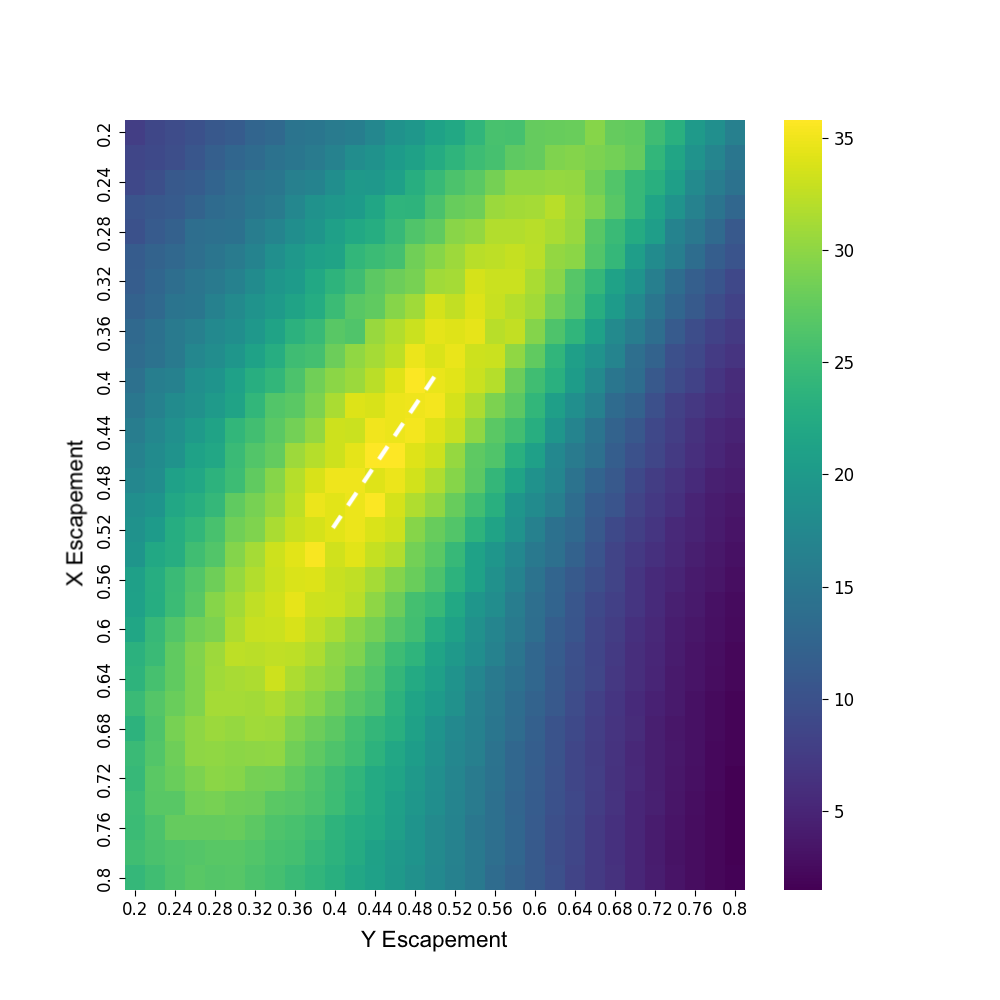
Tuning the CEsc strategy. This tuning procedure was analogous to that of the CMort strategy just summarized. Namely: A grid of 101 escapement values was laid out on the interval $[0,1]$ for Models 1 and 2; and a $51\times 51$ grid on $[0,1]^{2}$ was laid out for Models 3 and 4. Each grid point represented a CEsc policy. We used each of these policies to manage 100 replicate episodes. The optimal policy was the policy with the highest average reward obtained. A visualization of the tuning outcome for Model 4 is shown in Fig. 3.

Figure 3: Visualization of the cosntant escapement strategy tuning procedure for Model 4. There was a certain multiplicity in this tuning strategy: a “ridge of optimality” where policies had essentially equivalent behavior. Throughout our investigation, we tuned constant escapment in several occasions and, on each occassion, a different optimal policy along the ridge was found. The results for different policies along the ridge were in practice equivalent, with no discernible difference in performance. We highlighted the ridge with a white dotted line.

Parameter values used. The single-species model’s (eq. (3)) dynamic parameters were chosen as

$$r=K=1,\quad\beta=0.25,\quad c=0.1.$$ (7)

Here, the values of $\beta$ and $c$ were chosen as to make the system be roughly close to its tipping point.

For Models 2 and 3, their dynamic parameters (in eq. (4)) were chosen as follows

$$\begin{split}r_{X}=K_{X}=r_{Y}=K_{Y}=1,\quad\beta=0.3,\quad c=0.3\\ c_{XY}=0.1,\quad b=0.1,\quad D=1.1,\quad d_{Z}=0.1.\end{split}$$ (8)

Moreover, the variances for the stochastic terms were chosenas

$$\sigma^{2}(\eta_{X,t})=\sigma^{2}(\eta_{Y,t})=\sigma^{2}(\eta_{Z,t})=0.05.$$

For Model 4, we used $r_{X}(t)$ given as in eq. (5) and all other parameters were given as in eq. (8).

The values of $c$ and $\beta$ in the three-species model were slightly different than their values in the one-species model. These values were chosen heuristically: We observed that choosing the lower value of $c=0.1$ in this case would lead to quick near-extinction events even without a harvest. Moreover, $\beta$ was slightly increased simply to put more predation pressure on the $X$ and $Y$ populations and make them slightly more fragile.

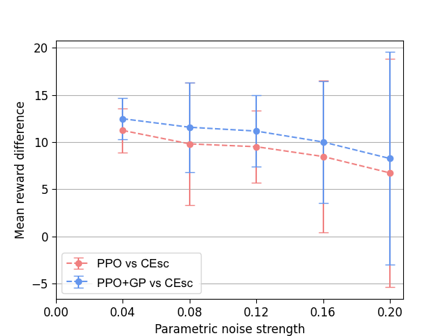
Stability analysis. To ensure that our results do not strongly depend on our parameter choices, we performed a stability analysis. Here, we perturbed parameters randomly and measured the difference in performance between our DRL-based methods and the CEsc strategy. We observed that the difference in performance is maintained for even relatively high noise strengths. We only considered the most complex case here, Model 4.

For each value of parametric noise strength $\sigma_{\text{param.}}$, we executed the following procedure: We sampled 100 choices of perturbed parameter values, where the perturbation was as follows—each parameter $P$ was perturbed to $(1+g_{P})P$ where $g_{P}$ was a Gaussian random variable with variance $\sigma_{\text{param.}}^{2}$. For each of these sample parameter sets, we tuned CEsc and trained the DRL agent. We measured the average reward difference between these two strategies for each of sample (this was done using 100 replicate evaluation episodes). Finally, we took the mean of this average difference over the 100 perturbed parameter samples.

The parametric noise strength values used were $[0.04,0.08,\dots,0.2]$.

5 Results

We evaluated each of the four management strategies considered on Models 1-4. To recap, the management strategies were CEsc, CMort, PPO and a Gaussian process interpolation of PPO (“PPO+G”). Furthermore, we characterized the trade-off between economic output and sustainability faced by CMort policies. This was done by evaluating CMort policies with a fraction of the optimal mortality rate (specifically, 80%, 90% and 95%). All evaluations were based on 100 replicate episodes.

We will visualize the results concerning Model 4 in this section, leaving the other models for App. A. This is the most complex scenario considered and where our results show the most compelling advantage of DRL methods with respect to classical strategies.

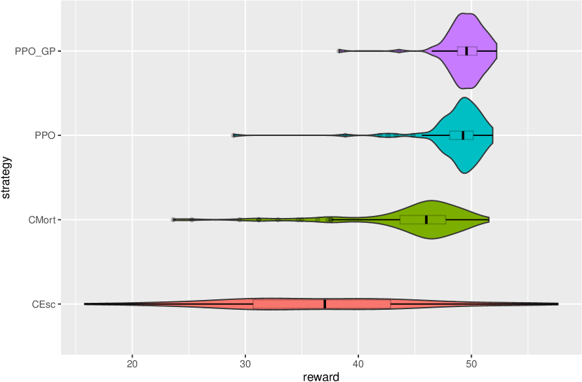
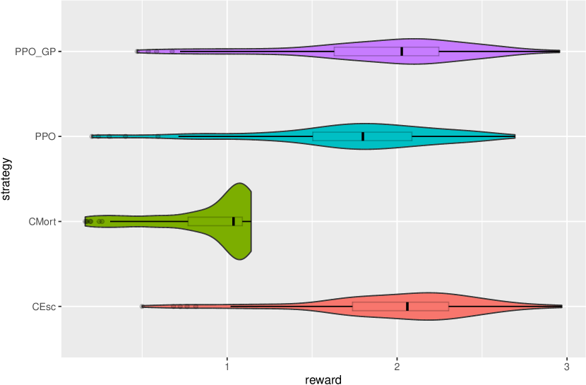
Our main result is summarized in Fig. 4 which displays the total reward distributions for the policy obtained through each strategy. Here we see that CEsc has a long-tailed distribution of rewards, and its average reward is much lower than other management strategies. CMort has a shorter-tailed distribution and a much higher average reward. Finally, both DRL-based strategies have a more concentrated reward distribution and a higher average reward than CMort.

Figure 4: Reward distributions for the four strategies considered. These are based on 100 evaluation episodes. We denote CEsc for constant escapement, CMort for constant mortality, PPO for the output policy of the PPO optimization algorithm, and PPO GP for the Gaussian process interpolation of the PPO policy.

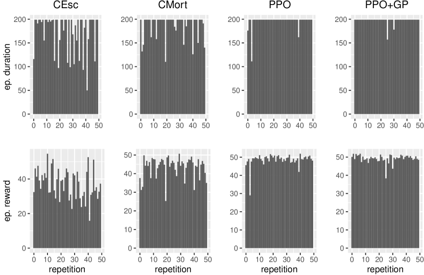
To assess what is the culprit for the classical strategies’ low performance with respect to the DRL-based strategies, we plot the duration of each of the 100 evaluation episodes of each strategy in Fig. 5. We see that early episode ends are prevalent in classical strategies and rare for DRL-based strategies. Early episode ends tend to happen at lower $t$ values for CEsc than CMort. Thus, distribution of episode durations seems to be widest for CEsc, followed by CMort, DRL and DRL+GP.

Figure 5: Hisotgrams of episode lengths and rewards for the four different management strategies considered. Only the first 50 evaluation episodes (from a total of 100) were included, for ease of visualization. From left to right, the four management strategies compared are CEsc, CMort, PPO, and PPO+GP.

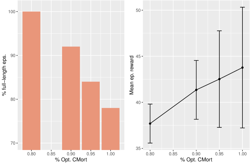
We examine the trade-off between profit and sustainability faced by the CMort strategy in Fig. 6. Two quantities are plotted: the fraction of evaluation episodes with maximal length (i.e. episodes with no near-extinction events), and the average reward. On the x-axis we have several sub-optimal mortality rates that err on the conservative side: e.g. the policy labeled “80% Opt. CMort” has the form

$$\pi:(X_{t},Y_{t},Z_{t})\mapsto(0.8M_{X}^{*},\ 0.8M_{Y}^{*}),$$

where $(M_{X}^{*},\ M_{Y}^{*})$ is the optimal CMort strategy. We see that sufficiently conservative policies attain high sustainability, but only at a high price in terms of profit. We expect a similar and, possibly, more pronounced effect for the CEsc strategy but do not analyze this case here.

Figure 6: Trade-off between reward and probability of a near-extinction event for CMort policies. We evaluated policies at the full optimal constant escapement value, and also at 0.8, 0.9, 0.95 of the latter. Each evaluation is based on 100 episodes. On the left we plot the percentage of episodes which last their maximum time window, i.e. that do not see a near-extinction event. On the right, we plot the mean episdoe reward and standard deviation for each policy.

One problem that is often encountered when using machine learning methods is the interpretability of the output of these methods. For our PPO strategy, the output is a policy function parametrized by a neural network $\theta$:

$$\pi_{\theta}:N_{t}\mapsto(M_{X}(N_{t}),M_{Y}(N_{t})),$$

where $N_{t}=(X_{t},Y_{t},Z_{t})$ is the state of the system at time $t$, and where $M_{X}$ and $M_{Y}$ are the mortalities due to harvest during that time-step. While the values of the neural network parameters are hard to interpret, the actual shape of the policy function is much more understandable.

Here we visualize the PPO+GP policy function and provide an interpretation for it, as this function is smoother and less noisy than the PPO policy function. The PPO policy function is visualized similarly in App. B.

Given its high dimension, it is not possible to fully display how the policy function obtained “looks like”—we thus project it down to certain relevant axes. The result of this procedure is shown in Fig. 7. In that figure, the shape of the optimal escapement strategy is provided for comparison.

Figure 7: Plots of the PPO+GP policy $\pi_{\text{PPO+GP}}$ along several relevant axes. Here $M_{X}$ and $M_{Y}$ are the $X$ and $Y$ components of the policy function. The values of the plots are generated in the following way: For each variable $X$, $Y$, and $Z$, the time-series of evaluation episodes are used to generate a window of typical values that variable attains when controlled by $\pi_{\text{PPO+GP}}$. Then, for each plot either $X$ or $Y$ was varied on $[0,1]$ along the $x$ axis, while the other variables (resp. $Y$ and $Z$, or $X$ and $Z$) were varied within the typical window computed before. The value of one of the latter two variables were visualized as color.

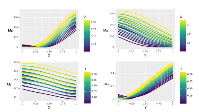
We notice that the DRL-derived policy has similarities to a CEsc policy. Here, the key difference is that the escapement value for each of the fished species is sensitive to variations in the other populations. This can be seen as color gradients in the plots of $(X,M_{X})$ and $(Y,M_{Y})$, where the gradient corresponds to differing values of $Z$. Moreover, this can be seen as an anti-correlation in the plot of $(X,M_{Y})$—for optimal CEsc, $M_{Y}$ is uncorrelated to $X$.

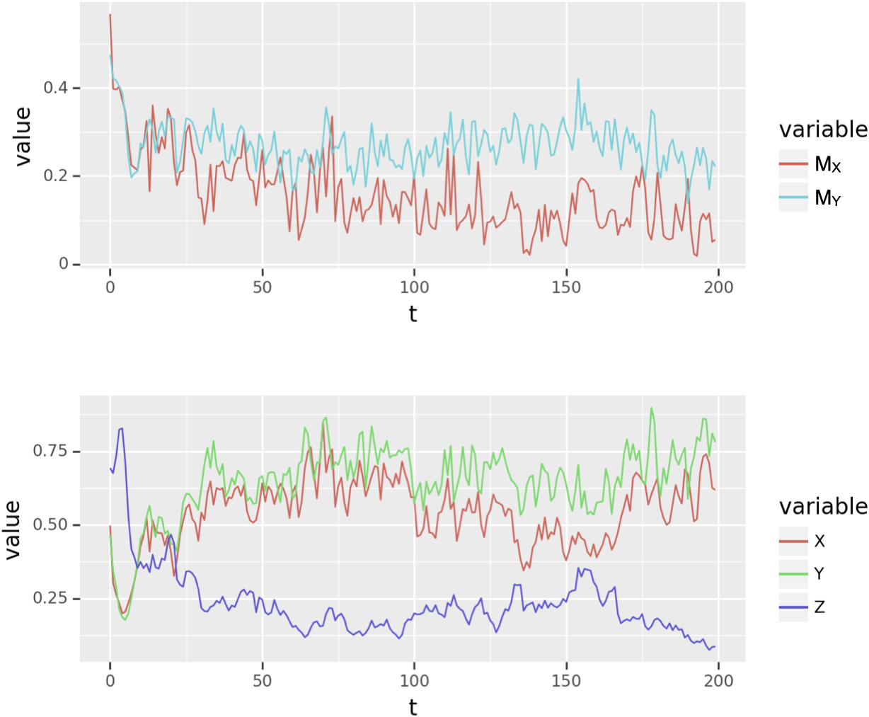
This sensitivity of the policy to, for instance, the values of $Z$ can be seen in the sample time series displayed in Fig. 8. Here, we can see that species $Z$ becomes endangered due to harvesting for all management strategies. The DRL-based strategy, however, is sensitive to the values of $Z$ and can respond accordingly by scaling the fishing effort with the value of $Z$. In particular, the policy responds to the period of diminishing values of $Z$ near the end of the episode, by restricting fishing on $X$ and $Y$, thus promoting $Z$’s growth. This pattern is rather common among the whole dataset—early episode ends are largely due to near-extinctions of $Z$ for all management strategies.

Figure 8: Time-series of an episode managed with $\pi_{\text{PPO+GP}}$. Here we plot the state of the system on the bottom panel, and the actions taken (fishing efforts on $X$ and $Y$—respectively $M_{X}$ and $M_{Y}$) on the top panel.

5.1 Recovering constant escapement for a single species

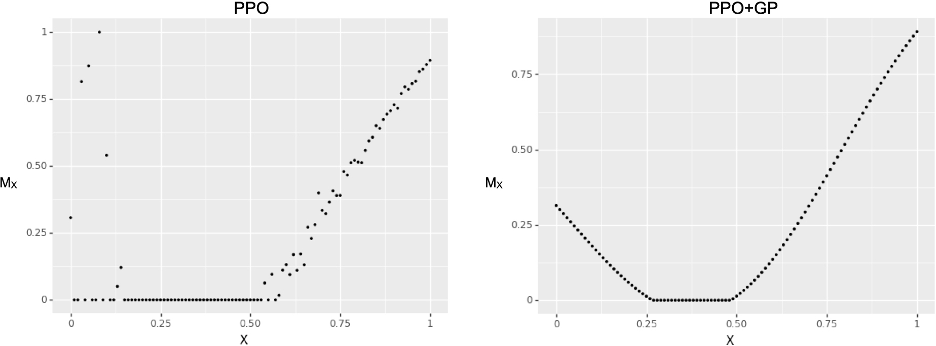
While the optimal control for our single-species model (3) can not be easily proven to be CEsc (since the right-hand side of that equation is not concave), from experience we can expect CEsc to either be optimal or near-optimal. We give evidence for this intuition by showing that our DRL method recovers a CEsc solution when trained. These results are shown in Fig. 9 Here we show both the output PPO policy, and its Gaussian process interpolation. This helps build an intuition about the relationship between our “PPO” and “PPO+GP” management strategies.

There is a presence of certain high-mortality points at low $X$ values in the PPO policy (which in turn generates a rising fishing mortality for $X$ values below a certain threshold in the PPO+GP policy). This is likely due to experience of near-extinctions early on in the training process—where, given an impending extinction, there is a higher reward for intensive fishing. These “jitters” are likely not fully erased through the optimization algorithm since near-extinction events become extremely rare after only a few training iterations. This way, the agent does not further explore that region of state space to generate new experience. We believe the most important aspect of the CEsc policy reproduced by PPO is the fact that there is some sufficiently-wide window below the threshold of the policy (i.e. below the optimal escapement value), on which no fishing is performed. That is, there exists some sufficiently large $\varepsilon$ such that if $X_{\text{thresh.}}$ is the optimal escapement value of the system, then $\pi_{PPO}(X)=0$ for all $X\in[X_{\text{thresh.}}-\varepsilon,\ X_{\text{thresh.}}]$.

Figure 9: Left panel: the policy obtained from 100 training iterations of the PPO algorithm on the “single species, single fishery” model. Right panel: the Gaussian process interpolation of the left panel. We plot both as scatter data evaluated on a 101-point grid on $[0,1]$, but these policies may of course be evaluated continuously—on any possible value of $X$.

5.2 Stability analysis

In this section we present results intended to show that the effects that we observe in this paper are not the result of a careful selection of parameter values, but rather arise for a wide variety of parameter values.

Our main result in this respect is Fig. 10. There, we plot the average episode reward difference between the two DRL-based methods we considered, and the optimal CEsc strategy. This figure shows that, for a wide range of parameter values, DRL-based strategies can have a considerable advantage over an optimized CEsc policy (the single-species optimal solution).

Figure 10: Mean reward difference between DRL methods (resp. our “PPO” and “PPO+GP” strategies), on the one hand, and the optimal constant escapement policy (“CEsc”) on the other. The dynamic parameters in eq. (4) were randomly perturbed from the values given in (8) according to the procedure detailed in Sec. 4. The noise strength of this perturbation is plotted as the x-axis. For each noise strength, 100 parameter perturbations were sampled—each one giving rise to a realization of the model. For each such realization, we optimized a CEsc policy and trained a PPO agent. Moreover, we interpolated the PPO policy using a Gaussian process, as detailed in Sec 4. Then, for each realization we compared the performance of these policies: we measured the mean reward difference betwen PPO and CEsc, and between PPO+GP and CEsc. The plot represents the distribution of reward differences observed at a given noise strength—we plot the mean and the standard deviation of the mean reward differences observed. In an equation, we plot the means $\mathbb{E}_{P}[\mu_{P}^{\text{DRL}}-\mu_{P}^{\text{CEsc}}]$, where $P$ are the paramter values, $\mu_{P}^{\text{DRL}}$ is the mean reward for a DRL policy trained on the problem with parameter values $P$, and, similarly, $\mu_{P}^{\text{CEsc}}$ is the mean reward of the optimal constant escpament policy for parameter values $P$.

6 Discussion

Fisheries are complex ecosystems, with interactions between species leading to highly non-linear dynamics. While current models for population estimation include many important aspects of this complexity, it is still common to use simplified dynamical models in order to guide decision making. This provides easily interpretable solutions, such as CMort policies. There is a drawback here, however: due to the simplicity of these dynamical models, the policies might not respond effectively in many situations—situations where the predictions of these simple models deviate considerably from reality. Because of this, policies such as MSY have faced pushback and are believed to have contributed to the depletion of fish stocks (Worm et al. 2006; Costello et al. 2016).

We propose an alternative approach to the problem of fishery control: to use a more expressive – albeit more complicated – dynamical model to guide decision making. Furthermore, rather than computing the optimal control policy for the model (something that is impossible in practice for complex systems), we use deep reinforcement learning to obtain a “pretty darn good” policy. This policy is estimated in a model-free setting, i.e., the agent treats the dynamical model (e.g. eq. (4)) as a black box of input-output pairs. By not relying on precise knowledge of the model’s parameter values, but rather just relying on input-output statistics, model-free approaches have gained traction in a variety of control theory settings (see, e.g., (Sato 2019; Ramirez, Yu, and Perrusquia 2022; Zeng et al. 2019)).

We compare deep reinforcement learning-based policies against classical management strategies (CMort and CEsc). While the latter are inspired by the shape of optimal solutions in the single-species setting, they are optimized in a model-free way as well: e.g. the optimal mortality rate is computed empirically from simulated data.

Because of the simplicity of the classical policy functions, the optimal such policy may be easily estimated through a grid-search. This is the case since these policy functions are only specified by one or two parameters (respectively in the single fishery, or two fishery cases). In contrast, DRL optimizes over the more expressive – and more complicated – family of policies parametrized by a neural network. Neural networks are often used as flexible function approximators that can be efficiently optimized over.

We showed that for sufficiently complex management scenarios – Models 3 and 4 – DRL-based management strategies perform significantly better than CEsc. This with respect to both average rewards received and conservation goals. In this sense, an approximate solution to a more complicated and expressive model, can outperform the optimal solution of the single-species problem—even when the parameters of the single-species solution are empirically optimized.

We found that the optimal CMort policy surprisingly performs much better than CEsc (Fig. 4). However, it can be observed in Fig. 6 that the CMort strategy faces a trade-off: high sustainability is achieved for sub-optimal mortality rates, but only at a significant decrease in the mean episode reward. We expect that with increasing ecosystem complexity this phenomenon might become more pronounced. We can understand this as a consequence of the rigidity of classical strategies: the simplicity of their expressions, depending only on a few parameters, means that policy optimization is constrained to a rather reduced subset of the space of possible policies.

The question of when multi-species models are well-approximated by single-species models was studied in detail in (Burgess et al. 2017). Here our approach is dual to that of the aforementioned paper. Rather than first optimizing a single-species model to approximate a more complex model and then finding the MSY value for the single-species model, we used simulated data to optimize CMort and CEsc directly on the three-species model. We do not investigate further whether our three-species models are well approximated by a single-species model in the sense of (Burgess et al. 2017). However: 1) Because the interaction terms in (4) are about an order of magnitude smaller than $r_{X}$ and $r_{Y}$, Models 2-4 are “close” in parameter-space to a single-species model. 2) The fact that for Model 2 all strategies match in performance suggests that (4) might be well-approximated by a single species model. This in turn suggests that the reason that DRL outperforms both single-species strategies for Models 3 and 4 is not due a lack of a single-species approximation for either $X$ or $Y$, but due to the complexity of having two harvested species. Moreover, the non-stationarity in Model 4 maintained the advantage of DRL over CEsc and CMort. Here, one may have expected an exacerbation of that advantage due to non-stationarities introducing biases to single-species approximate models (Burgess et al. 2017). We did, however, measure a decrease in the sustainability of CEsc in Model 4 with respect to Model 3.

Finally, we performed a stability analysis to ensure that the advantage of DRL-based techniques over CEsc is a ubiquitous phenomenon and not a result of a lucky selection of parameter values. We found (in Fig. 10) that an advantage can be observed even for relatively high-noise perturbations of the parameters—noise with a variance of 20% of the parameter values. The aforementioned Figure summarizes the statistics of 100 parameter perturbations so that we may expect perturbations of up to 60% (i.e. three sigmas) in the parameter values to appear in these statistics.

6.1 Future directions

There are a number of interesting directions that would be interseting to explore in future work.

First, benchmarking our results against increasingly more compex and realistic fishery models. This would include non-stationarities in the dynamical parameters to accurately reflect the effects of climate change on the ecosystem. This added complexity would likely pose a computational challenge—in future work we will likely need to test several different DRL training algorithms (see e.g. (Lapeyrolerie et al. 2022) for a non-exhaustive list), and it is very likely that hyperparameter tuning will need to be performed. Moreover, it may be that larger neural networks than the one we used in this research will be needed for the policy function. This all will mean that considerable technical work will be needed in order to make this next step computationally feasible (e.g. we might need to make more extensive use of GPUs and parallelization).

Second, to account for noisy estimates of the system’s state and imperfect policy implementation. This could be done straightforwardly, albeit it might increase the training time before DRL approaches converge, as well as introducing the need for hyperparameter tuning.

Third, to account for the systematic uncertainties behind the dynamics of the ecosystem—that is, to account for model biases with respect to reality. Here, one can employ tools from curriculum learning in order to train an agent that is generally capable of good management over a range of different dynamical models. This way, one can incorporate different models—expressing different aspects of the ecosystem—into the learning process of the agent. We believe that this step will likely be necessary if DRL algorithms are to be applied successfully in the fishery management problem. Curriculum learning is rather expensive computationally, however, and involves a non-trivial curriculum design which will guide the agent in its learning process. This way, considerable technical work would be needed for this direction.

6.2 Acknowledgements

The title of this piece references a mathematical biology workshop at NIMBioS organized by Paul Armsworth, Alan Hastings, Megan Donahue, and Carl Towes in 2011 which first sought to emphasize ‘pretty darn good’ control solutions to more realistic problems over optimal control to idealized ones. This material is based upon work supported by the National Science Foundation under Grant No. DBI-1942280.

Appendix A Appendix: Results for stationary models

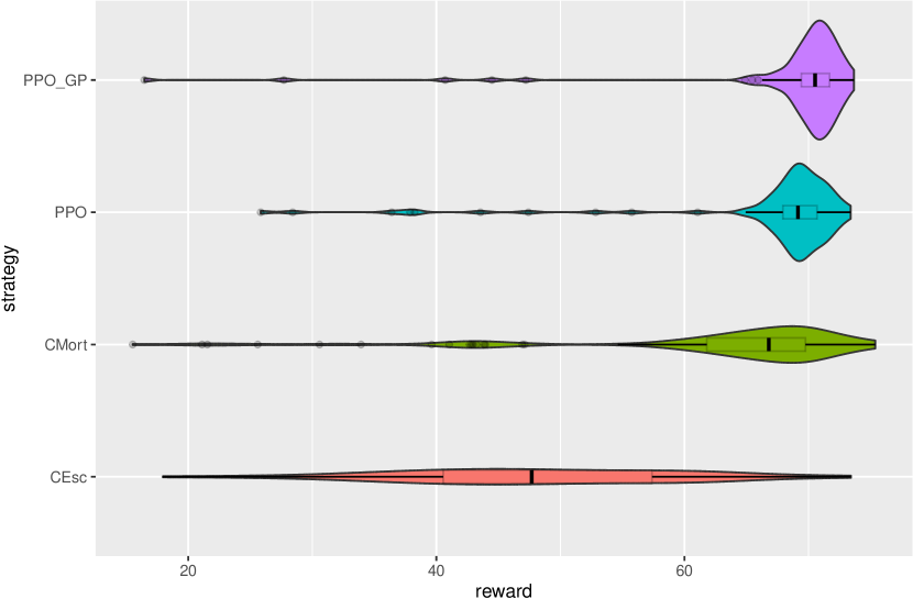
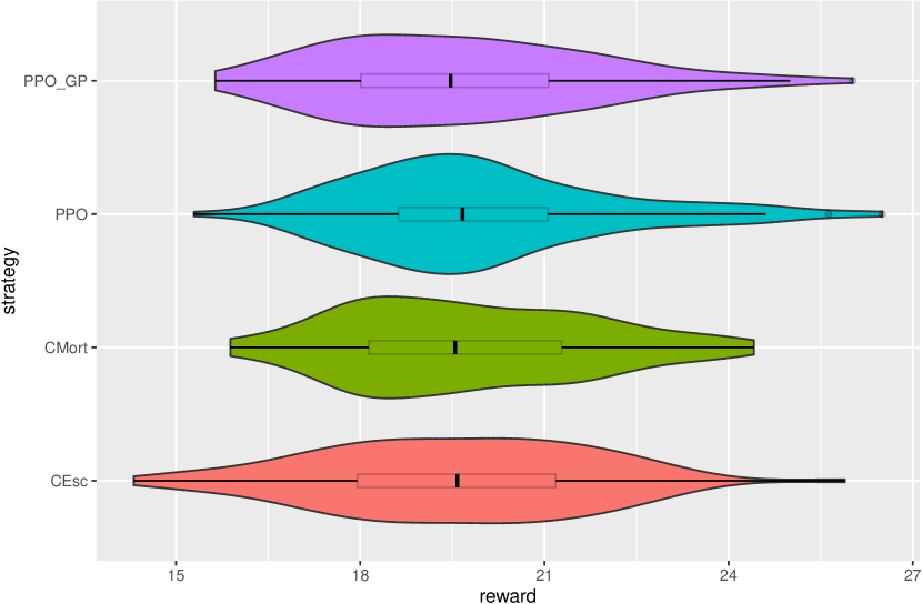
In the main text we focused on the non-stationary model (“three species, two fisheries, non-stationary” in Table 1) for the sake of space and because our results were most compelling there. Here we present the reward distributions for the other models considered—the three stationary models, lines 1-3 in Table 1. These results are shown in Figs. 11, 12 and 13.

Figure 11: Reward distributions for the four strategies considered. These are based on 100 evaluation episodes of Model 3 in Table 1. We denote CEsc for constant escapement, CMort for constant mortality, PPO for the output policy of the PPO optimization algorithm, and PPO GP for the Gaussian process interpolation of the PPO policy.

Figure 12: Reward distributions for the four strategies considered. These are based on 100 evaluation episodes of Model 2 in Table 1. We denote CEsc for constant escapement, CMort for constant mortality, PPO for the output policy of the PPO optimization algorithm, and PPO GP for the Gaussian process interpolation of the PPO policy.

Figure 13: Reward distributions for the four strategies considered. These are based on 100 evaluation episodes of Model 1 in Table 1. We denote CEsc for constant escapement, CMort for constant mortality, PPO for the output policy of the PPO optimization algorithm, and PPO GP for the Gaussian process interpolation of the PPO policy.

Appendix B Appendix: PPO policy function for non-stationary model

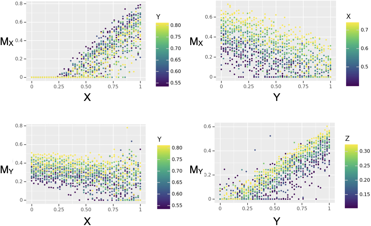
In the main text, Fig. 7, we presented a visualization of the PPO+GP policy function obtained for the “three species, two fisheries, non-stationary” model. This policy function is a Gaussian process regression of scatter data of the PPO policy function. In Fig. 14 we present a representation of this scatter data in a similar format as Fig. 7.

Figure 14: Plots of the PPO policy $\pi_{\text{PPO}}$ along several relevant axes. Here $M_{X}$ and $M_{Y}$ are the $X$ and $Y$ components of the policy function. The values of the plots are generated in the following way: For each variable $X$, $Y$, and $Z$, the time-series of evaluation episodes are used to generate a window of typical values that variable attains when controlled by $\pi_{\text{PPO}}$. Then, for each plot either $X$ or $Y$ was evaluated on 100 values in $[0,1]$ along the $x$ axis, while the other variables (resp. $Y$ and $Z$, or $X$ and $Z$) were varied within the typical window computed before. Within this window, 5 values are used. The value of one of the latter two variables were visualized as color. This scatter data was used as an input to generate $\pi_{\text{PPO+GP}}$, visualized in the main text.

Appendix C Appendix: Gaussian process interpolation

Here we summarize the procedure used to interpolate the PPO policy (visualized in Fig. 14). We use the GaussianProcessRegressor object of the sklearn Python library with a kernel given by

$$\text{RBF}(\text{length scale = 10})+\text{WhiteNoise}(\text{noise level = 0.1}).$$

This interpolation method is applied to scatter data of the PPO policy evaluated on 3 different grids on $(X,Y,Z)$ states: $G_{X}$, a $51\times 5\times 5$ grid; $G_{Y}$, a $5\times 51\times 5$ grid; and $G_{Z}$, a $5\times 5\times 51$ grid. This combination of grids was used instead of a single dense grid in order to reduce the computational intensity of the interpolation procedure. For $G_{X}$, the 5 values for $Y$ and $Z$ were varied in a “popular window,” i.e. episode time-series data was used to determine windows of $Y$ and $Z$ values which were most likely. The grids $G_{Y}$ and $G_{Z}$ were generated in a similar fashion, mutatis mutandis. The length scale and noise level values of this kernel were chosen arbitrarily—no hyperparameter tuning was needed to produce satisfactory interpolation, as will be shown in the results section.

References

reAnderson, Brian DO, and John B Moore. 2007. Optimal Control: Linear Quadratic Methods. Courier Corporation.

preBellemare, Marc G, Yavar Naddaf, Joel Veness, and Michael Bowling. 2013. “The Arcade Learning Environment: An Evaluation Platform for General Agents.” Journal of Artificial Intelligence Research 47: 253–79.

preBurgess, Matthew G, Henrique C Giacomini, Cody S Szuwalski, Christopher Costello, and Steven D Gaines. 2017. “Describing Ecosystem Contexts with Single-Species Models: A Theoretical Synthesis for Fisheries.” Fish and Fisheries 18 (2): 264–84.

preChapman, Melissa, Lily Xu, Marcus Lapeyrolerie, and Carl Boettiger. 2023. “Bridging Adaptive Management and Reinforcement Learning for More Robust Decisions.” Philosophical Transactions of the Royal Society B (Accepted).

preClark, Colin W. 1990. Mathematical Bioeconomics: The Optimal Management of Renewable Resources, 2nd Edition. Wiley-Interscience.

preClark, Colin W. 1973. “Profit Maximization and the Extinction of Animal Species.” Journal of Political Economy 81 (4): 950–61. https://doi.org/10.1086/260090.

preCollins, MSFB, SFB Tett, and C Cooper. 2001. “The Internal Climate Variability of HadCM3, a Version of the Hadley Centre Coupled Model Without Flux Adjustments.” Climate Dynamics 17: 61–81.

preCostello, Christopher, Daniel Ovando, Tyler Clavelle, C. Kent Strauss, Ray Hilborn, Michael C. Melnychuk, Trevor A Branch, et al. 2016. “Global fishery prospects under contrasting management regimes.” Proceedings of the National Academy of Sciences 113 (18): 5125–29. https://doi.org/10.1073/pnas.1520420113.

preDegrave, Jonas, Federico Felici, Jonas Buchli, Michael Neunert, Brendan Tracey, Francesco Carpanese, Timo Ewalds, et al. 2022. “Magnetic Control of Tokamak Plasmas Through Deep Reinforcement Learning.” Nature 602 (7897): 414–19.

preFrançois-Lavet, Vincent, Peter Henderson, Riashat Islam, Marc G Bellemare, Joelle Pineau, et al. 2018. “An Introduction to Deep Reinforcement Learning.” Foundations and Trends® in Machine Learning 11 (3-4): 219–354.

preGordon, Chris, Claire Cooper, Catherine A Senior, Helene Banks, Jonathan M Gregory, Timonthy C Johns, John FB Mitchell, and Richard A Wood. 2000. “The Simulation of SST, Sea Ice Extents and Ocean Heat Transports in a Version of the Hadley Centre Coupled Model Without Flux Adjustments.” Climate Dynamics 16: 147–68.

preGordon, H. Scott, and Chicago Press. 1954. “The Economic Theory of a Common-Property Resource: The Fishery.” Journal of Political Economy 62 (2): 124–42. https://doi.org/10.1086/257497.

preJanner, Michael, Justin Fu, Marvin Zhang, and Sergey Levine. 2019. “When to Trust Your Model: Model-Based Policy Optimization.” arXiv:1906.08253 [Cs, Stat], November. http://arxiv.org/abs/1906.08253.

preLapeyrolerie, Marcus, Melissa S Chapman, Kari EA Norman, and Carl Boettiger. 2022. “Deep Reinforcement Learning for Conservation Decisions.” Methods in Ecology and Evolution 13 (11): 2649–62.

preMangel, Marc. 2006. The Theoretical Biologist’s Toolbox: Quantitative Methods for Ecology and Evolutionary Biology. Cambridge University Press.

preMarescot, Lucile, Guillaume Chapron, Iadine Chadès, Paul L. Fackler, Christophe Duchamp, Eric Marboutin, and Olivier Gimenez. 2013. “Complex Decisions Made Simple: A Primer on Stochastic Dynamic Programming.” Methods in Ecology and Evolution 4 (9): 872–84. https://doi.org/10.1111/2041-210X.12082.

preMay, Robert M. 1977. “Thresholds and Breakpoints in Ecosystems with a Multiplicity of Stable States.” Nature 269 (5628): 471–77.

preMnih, Volodymyr, Koray Kavukcuoglu, David Silver, Alex Graves, Ioannis Antonoglou, Daan Wierstra, and Martin Riedmiller. 2013. “Playing Atari with Deep Reinforcement Learning.” arXiv Preprint arXiv:1312.5602.

preMoerland, Thomas M, Joost Broekens, Aske Plaat, Catholijn M Jonker, et al. 2023. “Model-Based Reinforcement Learning: A Survey.” Foundations and Trends® in Machine Learning 16 (1): 1–118.

preOpenAI. 2022. “ChatGPT: Optimizing Language Models for Dialogue.” https://openai.com/blog/chatgpt/.

prePolydoros, Athanasios S, and Lazaros Nalpantidis. 2017. “Survey of Model-Based Reinforcement Learning: Applications on Robotics.” Journal of Intelligent & Robotic Systems 86 (2): 153–73.

prePope, VD, ML Gallani, PR Rowntree, and RA Stratton. 2000. “The Impact of New Physical Parametrizations in the Hadley Centre Climate Model: HadAM3.” Climate Dynamics 16: 123–46.

prePunt, André E, Doug S Butterworth, Carryn L de Moor, José A A De Oliveira, and Malcolm Haddon. 2016. “Management strategy evaluation: best practices.” Fish and Fisheries 17 (2): 303–34. https://doi.org/10.1111/faf.12104.

preRAM Legacy Stock Assessment Database. 2020. “RAM Legacy Stock Assessment Database V4.491.” https://doi.org/10.5281/zenodo.3676088.

preRamirez, Jorge, Wen Yu, and Adolfo Perrusquia. 2022. “Model-Free Reinforcement Learning from Expert Demonstrations: A Survey.” Artificial Intelligence Review, 1–29.

preRiahi, Keywan, Detlef P Van Vuuren, Elmar Kriegler, Jae Edmonds, Brian C O’neill, Shinichiro Fujimori, Nico Bauer, et al. 2017. “The Shared Socioeconomic Pathways and Their Energy, Land Use, and Greenhouse Gas Emissions Implications: An Overview.” Global Environmental Change 42: 153–68.

preSato, Yoshiharu. 2019. “Model-Free Reinforcement Learning for Financial Portfolios: A Brief Survey.” arXiv Preprint arXiv:1904.04973.

preSchaefer, Milner B. 1954. “Some aspects of the dynamics of populations important to the management of the commercial marine fisheries.” Bulletin of the Inter-American Tropical Tuna Commission 1 (2): 27–56. https://doi.org/10.1007/BF02464432.

preSeo, J, Y-S Na, B Kim, CY Lee, MS Park, SJ Park, and YH Lee. 2022. “Development of an Operation Trajectory Design Algorithm for Control of Multiple 0D Parameters Using Deep Reinforcement Learning in KSTAR.” Nuclear Fusion 62 (8): 086049.

preSethi, Suresh P, and Suresh P Sethi. 2019. What Is Optimal Control Theory? Springer.

preWorm, Boris, Edward B Barbier, Nicola Beaumont, J Emmett Duffy, Carl Folke, Benjamin S Halpern, Jeremy B C Jackson, et al. 2006. “Impacts of biodiversity loss on ocean ecosystem services.” Science (New York, N.Y.) 314 (5800): 787–90. https://doi.org/10.1126/science.1132294.

preZeng, Deze, Lin Gu, Shengli Pan, Jingjing Cai, and Song Guo. 2019. “Resource Management at the Network Edge: A Deep Reinforcement Learning Approach.” IEEE Network 33 (3): 26–33.

preZhang, Yinyan, Shuai Li, and Liefa Liao. 2019. “Near-Optimal Control of Nonlinear Dynamical Systems: A Brief Survey.” Annual Reviews in Control 47: 71–80.

p