AdvisingNets: Learning to Distinguish Correct and Wrong Classifications
via Nearest-Neighbor Explanations

Abstract

Besides providing insights into how an image classifier makes its predictions, nearest-neighbor examples also help humans make more accurate decisions. Yet, leveraging this type of explanation to improve both human-AI team accuracy and classifier’s accuracy remains an open question. In this paper, we aim to increase both types of accuracy by (1) comparing the input image with post-hoc, nearest-neighbor explanations using a novel network (AdvisingNet), and (2) employing a new reranking algorithm. Over different baseline models, our method consistently improves the image classification accuracy on CUB-200 and Cars-196 datasets. Interestingly, we also reach the state-of-the-art human-AI team accuracy on CUB-200 where both humans and an AdvisingNet make decisions on complementary subsets of images.

1 Introduction

A goal of Explainable AI (XAI) is to provide humans with insights to evaluate the predictions of classifiers. By examining how a model “reasons” about a given input, users can better decide whether a classifier makes a correct prediction or not (Chen et al. 2023a). In computer vision, this is a non-trivial task and many explanation methods (such as feature-attribution maps) fail to improve human accuracy (Jin, Li, and Hamarneh 2021, 2022; Nguyen, Kim, and Nguyen 2021; Kim et al. 2023a).

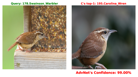
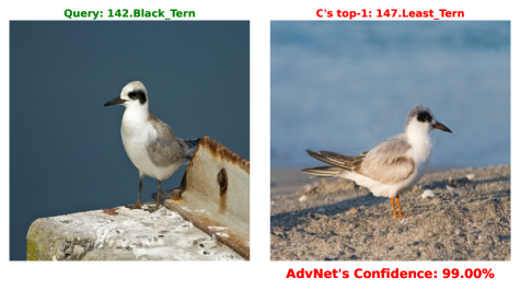
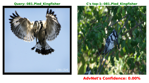
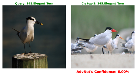
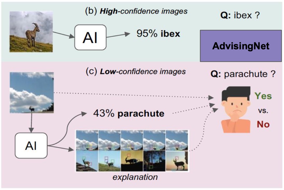
In contrast, there is growing evidence demonstrating the effectiveness of example-based explanations in improving human decisions, particularly when using techniques like nearest neighbors (NNs) (Papernot and McDaniel 2018; Nguyen, Kim, and Nguyen 2021; Liu et al. 2022; Chen et al. 2023b). Intuitively, if the input image is more similar to its nearest neighbors (NNs) from the classifier’s top-1 predicted class than those from the other classes, then the top-1 label should be correct and so accepted by human users (see Fig. 1). Otherwise, the top-1 label should be incorrect and rejected by users.

Figure 1: Given an input image $x$ and a pretrained, frozen (denoted by a ) classifier $\mathbf{C}$ that predicts the output for $x$, humans can discern whether the model has made a correct prediction or not by comparing $x$ with its training-set nearest neighbors (NN), derived from the predicted classes (Nguyen, Kim, and Nguyen 2021). In this paper, we train AdvisingNets to mimic humans and to choose Painted Bunting over the Indigo Bunting label for this example.

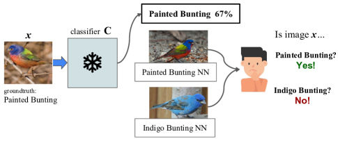
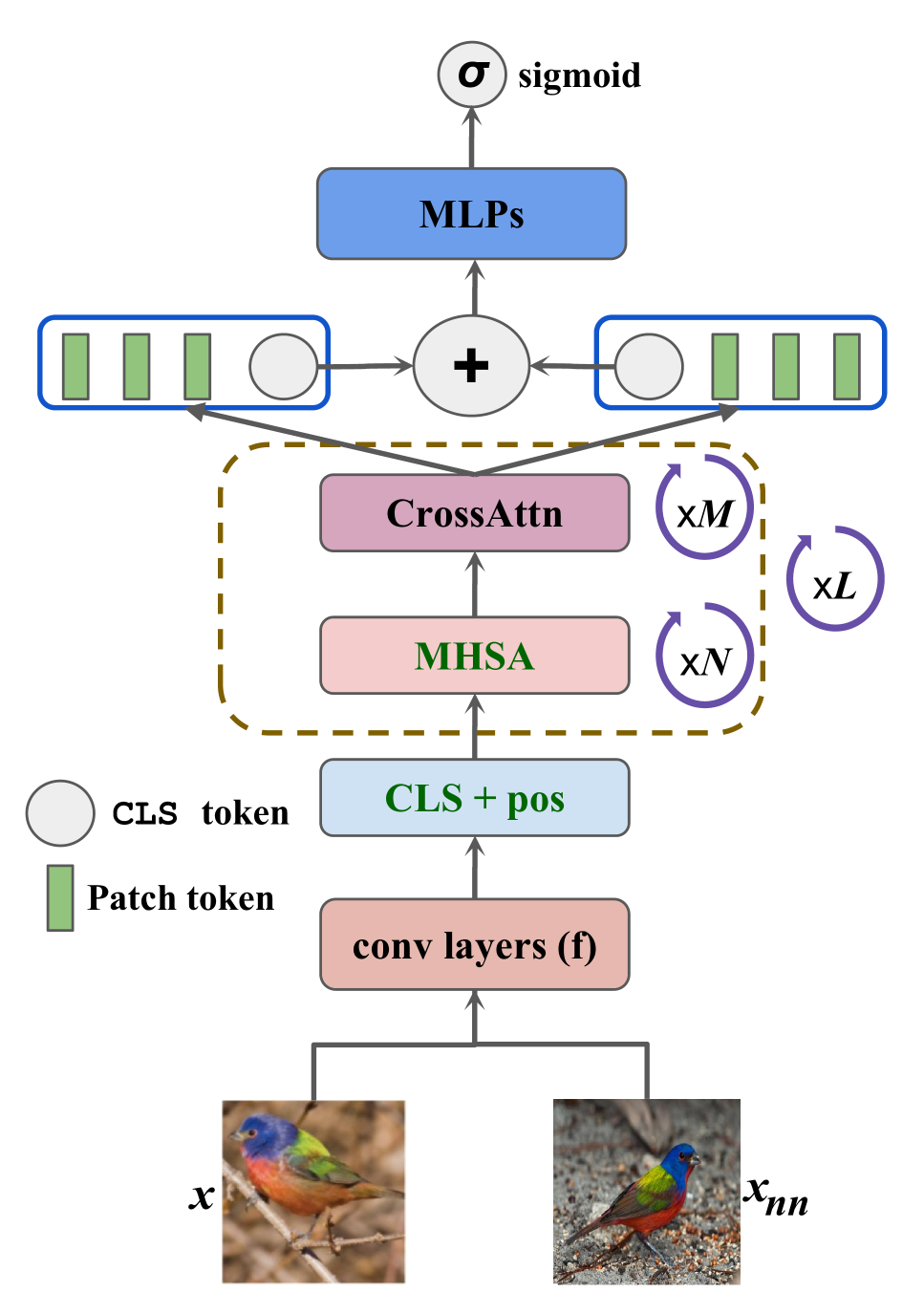
Inspired by this idea, we train a VisionTransformer-based classifier called AdvisingNet (Fig. 2(b)) that predicts whether the output label of a given classification model is correct or wrong by comparing the input image with its nearest neighbors.

To train AdvisingNets, we propose a novel sampling procedure to generate image pairs, which consist of the input image and its nearest neighbors derived from both the ground-truth and the other classes. We demonstrate the utility of AdvisingNets on fine-grained CUB-200 (Wah et al. 2011) and Cars-196 (Krause et al. 2013) classification tasks. Our main findings are:

• On CUB-200, AdvisingNets achieve up to 90.63% in predicting correct vs. wrong predictions, surpassing the human baseline by +25.88 points (pts), an optimized AI agent by +3.23 pts, and a team of human+AI by +4.80 pts (Table 1).

• We propose an algorithm called Top-class Reranking (TCR) that re-ranks the top-predicted classes of pretrained classifiers. TCR improves the accuracy of a bird classifier (based on an iNaturalist-pretrained ResNet-50 backbone) by +2.17 pts on CUB-200 (Table 2) and a car classifier (based on ImageNet-pretrained ResNet-50 backbone) by +0.64 pts on Cars-196 (Table 3). On CUB, our method also outperforms other prototype-based classifiers, such as prototypical part-based (e.g., ProtoPNet) and visual correspondence-based classifiers.

• We find that AdvisingNets when used with TCR do not only improve the accuracy of target classifiers seen during training but also unseen classifiers plugged in during test time. We find that the effectiveness of AdvisingNets generalizes over different target classifiers (when using TCR), different network architectures, and the number of nearest neighbors.

2 Framework

We first present the details for training AdvisingNets and their two downstream tasks.

2.1 Training AdvisingNets

Problem formulation

Assessing whether a classifier’s prediction is correct or not is an inherent task that every stakeholder needs to perform when working on high-stakes AI applications. Inspired by prior work that shows the effectiveness of NN examples for humans to classify machine predictions (Fig. 1), we reduce the task from distinguishing between correct and incorrect predictions into assessing whether the input image $x$ and its NNs from predicted classes are of the same class (i.e., similarity prediction).

Let $\mathbf{C}$ be an image classifier that transforms an image $x$ into a softmax probability distribution $\mathbf{P}$ over all classes. $x$ has a ground-truth label $y$ (e.g. Painted Bunting in CUB; Fig. 1).

Let $A$ be a binary, image-comparison classifier that takes in two images and predicts whether they belong to the same class (Fig. 2(b)). We call this classifier an AdvisingNet because when coupled with the TCR algorithm, we can improve $\mathbf{C}$’s predictions by pinpointing the ground-truth label that is probable to be among the top-predicted classes (Sec. 2.2).

Let $\mathbf{T}$ be a set of top-ranked classes in $\mathbf{P}$. From each class in $\mathbf{T}$, we retrieve the nearest neighbors $x_{nn}$ of $x$ to establish image pairs $(x,x_{nn})$ for training $A$. The pair is labeled 1 (positive) if $x_{nn}$ is selected from the groundtruth class $y$. Otherwise, for a negative pair having label 0, $x_{nn}$ is sampled from a class different from $y$ (Fig. 2(a)). For each pair $(x,x_{nn})$, $A$ computes a logit score $s\in\mathbb{R}$, which is then converted into a probability using a sigmoid function, $\hat{y}=\sigma(s)$, where $\sigma(s)=\frac{1}{1+e^{-s}}$. The resulting value, a probability, is thresholded at 0.5 to yield the final binary classification (see Fig. 2(b)).

With $B$ training samples, and a true binary label $y_{i}$ (Accept or Reject) for each $i$-th sample pair, we train $A$ to minimize the following binary cross-entropy (BCE) loss:

$$L_{BCE}=-\frac{1}{B}\sum_{i=1}^{B}y_{i}\log(\sigma(s_{i}))+(1-y_{i})\log(1-\sigma(s_{i}))$$ (1)

Sampling positive and negative neighbors

Given an input image $x$, instead of randomly picking NNs for generating $(x,x_{nn})$ pairs, we propose a novel sampling method that selectively chooses $x_{nn}$ based on the output of the pre-trained model $\mathbf{C}$ on $x$ as shown in Fig. 2(a).

For each image in the top-$Q$ classes, we mark the $(x,x_{nn})$ pairs as positive (+) or negative (–) accordingly, depending on whether the ground-truth label of $x$ matches these classes (see Fig. 2(a)).

To help AdvisingNets detect subtle differences between similar-looking species (which are more often misclassified and co-present in the top-predicted classes (Taesiri et al. 2023)), we consider only the top-$Q$ classes (empirically, $Q\in\{3,5,10,15\}$) returned by the classifier $C$ for an input $x$. NNs taken from classes outside the top-$Q$ are often clearly different from the input $x$ and do not serve as hard negatives.

(a) Sampling positive and negative pairs for training AdvisingNets

(b) AdvisingNet architecture

Figure 2: (a) Our sampling method generates positive and negative pairs based on top-predicted labels on $x$ from a pre-trained, frozen () classifier $\mathbf{C}$. In this example, the ground-truth label of $x$ is Painted Bunting, which matches the top-1 class, yielding $K$ positive pairs. In contrast, $Q-1$ classes do not match the ground-truth label and each provides a negative pair. Ultimately, this forms a collective $Q+K-1$ pairs per sample $x$ for the training of AdvisingNets. (b) AdvisingNet architecture consists of both convolutional and Transformer layers. The network processes a pair of images $(x,x_{nn})$ as input and produces a score $\mathbf{s}\in\mathbb{R}$. This score is subsequently passed through a sigmoid layer $\mathbf{\sigma}$ to determine if the images are of the same class. $L$, $M$, and $N$ are the depths of the corresponding blocks.

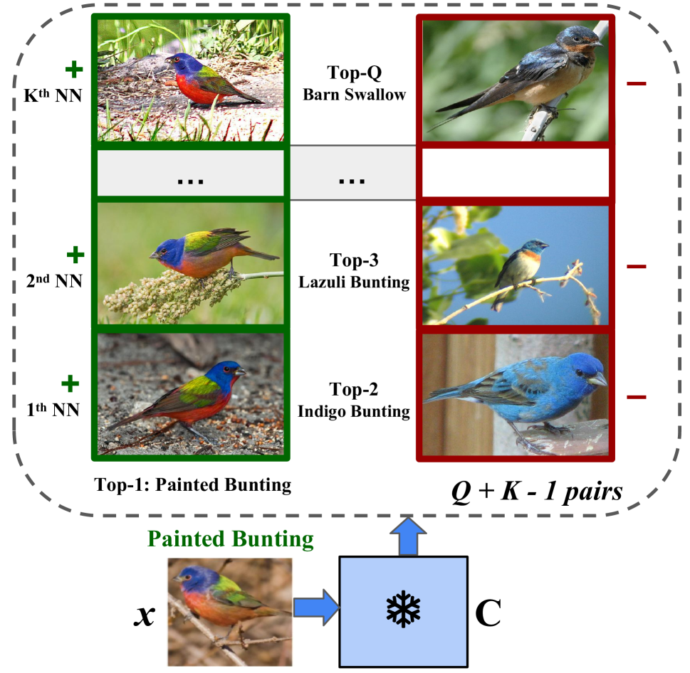
With one image per class, this sampling strategy yields at most 1 positive instance and at least $Q-1$ negative instances (e.g., $Q$ negative instances if the ground-truth label does not appear in the top $Q$ classes). Given that $x$ is previously part of the training set for classifier $\mathbf{C}$, it is likely that the top-1 predicted class matches the ground-truth label. To increase the number of positive samples and help AdvisingNets deal with inter-class variations, we sample $K$ neighbors from the top-1 class to derive $K$ positive pairs.

The retrieved nearest neighbors are ranked based on the Euclidean distances (using faiss framework) between their embeddings (i.e., the average pooling features of the last conv layer of $\mathbf{C}$) and that of the input image. Note that the first nearest neighbor from the ground-truth class is typically the same with $x$ itself. As such, we exclude this pair.

For each sample $x$, we thus form $Q+K-1$ pairs for training AdvisingNets. When the top-1 predicted class matches the ground-truth label, our method generates K positive pairs and $Q-1$ negative pairs. In contrast, when the top-1 predicted class does not match the ground-truth label, we obtain a minimum of $Q+K-2$ negative pairs and a maximum of one positive pair. Refer to Sec. A12 for examples of training pairs .

Hybrid architecture

AdvisingNets harness the power of both convolutional and Transformer layers (Fig. 2(b)). We initialize the convolutional layers with pretrained weights from $\mathbf{C}$ to encode input images. For the Transformer layers, we adopt the CrossViT backbone (Chen, Fan, and Panda 2021) for comparing the features between two images. The two branches correspond to the two input images fed into AdvisingNets. Different from CrossViT, our two branches handle the same image scale and share the weights, which makes AdvisingNets more compact. We also exclude the linear projection in conventional ViT (Dosovitskiy et al. 2020) as the conv layers are already able to provide patch-level tokens. In sum, the layers of AdvisingNets are:

$$\mathbf{x}_{\text{conv1 }}=\mathbf{f}\left(\mathbf{x}\right);~{}~{}~{}~{}~{}~{}\mathbf{x}_{\text{conv2 }}=\mathbf{f}\left(\mathbf{x}_{nn}\right)$$ (2)

$$\mathbf{x}_{1}=\left[\mathbf{x}_{cls}\|\mathbf{x}_{\text{conv1 }}\right]+\mathbf{x}_{\text{pos }};\mathbf{x}_{2}=\left[\mathbf{x}_{cls}\|\mathbf{x}_{\text{conv2 }}\right]+\mathbf{x}_{\text{pos }}$$

$$\mathbf{y}_{1}=\mathbf{x}_{1}+\mathbf{MHSA}(\mathbf{x}_{1});\mathbf{y}_{2}=\mathbf{x}_{2}+\mathbf{MHSA}(\mathbf{x}_{2})$$

$$\mathbf{z1,z2}=\mathbf{CrossAttn}\left(\mathbf{y}_{1},\mathbf{y}_{2}\right)$$

$$\mathbf{o}=\mathbf{concat}\left(\mathbf{z}_{1}[0,:],\mathbf{z}_{2}[0,:]\right)$$

$$\mathbf{s}=\mathbf{MLPs}\left(\mathbf{o}\right)$$

First, output of the conv layers $\mathbf{f}$ has a shape of $\mathbb{R}^{D\times H\times W}$, where $D$ is the number of convolution channels. $\mathbf{x}_{cls}\in\mathbb{R}^{1\times D}$ and $\mathbf{x}_{\text{pos }}\in\mathbb{R}^{(1+N)\times D}$ are CLS token and positional embedding, respectively.

Each image is represented by $H\times W$ patch tokens with a dimension of $D$. We flatten and transpose the conv feature vectors of two images to get $\mathbf{x}_{\text{conv1}}$, $\mathbf{x}_{\text{conv2}}$$\in\mathbb{R}^{N\times D}$ (e.g., $N=49$ and $D=2048$ for ResNet-50 conv4). After adding CLS token and positional embedding, the two encoded images $\mathbf{x}_{1}$ and $\mathbf{x}_{2}$ $\in\mathbb{R}^{(1+N)\times D}$ are put into the Transformer layers. $\operatorname{MHSA}$ is the self-attention operator and $\operatorname{CrossAttn}$ denotes the Cross-Attention token fusion approach in CrossViT, producing $\mathbf{y}_{1}$ $\mathbf{y}_{2}$, and $\mathbf{z}_{1}$ $\mathbf{z}_{2}$ $\in\mathbb{R}^{(1+N)\times D}$. Then, we extract the CLS tokens from $\mathbf{z}_{1}$ $\mathbf{z}_{2}$ and concatenate to generate $\mathbf{o}\in\mathbb{R}^{2\times D}$, which serves as input for multilayer perceptrons (MLPs). The MLPs output a logit score $\mathbf{s}\in\mathbb{R}$ that quantifies the degree of similarity between the two input images. Finally, a sigmoid layer is applied to achieve the confidence score for the classifier. Thresholding is performed at $0.5$ to yield binary predictions.

2.2 Downstream applications of AdvisingNets

Task 1: Human-AI teaming on Accepting/Rejecting AI decisions

We follow the experimental setups for human-AI collaboration from (Taesiri, Nguyen, and Nguyen 2022), where humans and AIs work on complementary image subsets to accept and reject a pretrained model’s predictions. In the original setup, a confidence threshold was computed to determine for which instances the human or the AI should be making decisions so that the AI would only make decisions for instances it was most confident on. Our approach substitutes the naive AI agent, referred to as Thresholding, with the AdvisingNet (see Sec. A4 for further details).

Task 2: Single-label image classification

While AdvisingNets can differentiate correct and incorrect predictions of a pretrained classifier $\mathbf{C}$, we study how to use them to improve $\mathbf{C}$ in image classification tasks. We introduce an algorithm called Top-classes Reranking or TCR (Algorithm 1), which re-ranks the top-predicted classes, initially given by $\mathbf{C}$. Specifically, upon receiving an image $x$, $\mathbf{C}$ makes an initial set of predictions $\mathbf{P}$. The top-$Q$ classes are selected for re-ranking (L2–4), where for each of class, AdvisingNet computes a confidence score between the input image $x$ and the representative image of the class (the closest NN). The class that yields the highest confidence score is chosen as the final predicted class for the input image (L9–20).

Algorithm 1 Top-classes Reranking

0:  Image $x$, Pretrained classifier $\mathbf{C}$, AdvisingNet $A$, Number of top classes to consider $Q$

0:  Reranked top-Q classes $\mathbf{T^{\prime}}$ and top-1 predicted class $\hat{y}$ after re-ranking

1:  // Get initial predictions from the pretrained classifier

2:  $\mathbf{P}\leftarrow\mathbf{C}(x)$

3:  // Select top Q classes from $\mathbf{P}$

4:  $\mathbf{T}\leftarrow\text{TopQClasses}(\mathbf{P},Q)$

5:  // Initialize a list to store re-ranked classes with scores

6:  $\mathbf{R}\leftarrow$ empty list

7:  // Loop over top Q classes

8:  for $\text{class}\in\mathbf{T}$ do

9:     // Obtain a representative image for the class

10:     $\text{rep\_image}\leftarrow\text{GetRepresentativeImage}(\text{class})$

11:     // Compute confidence score

12:     $\text{confidence\_score}\leftarrow A(x,\text{rep\_image})$

13:     // Store the class and its confidence score

14:     Append $(\text{class},\text{confidence\_score})$ to $\mathbf{R}$

15:  end for

16:  // Rerank the classes based on confidence scores

17:  $\mathbf{T^{\prime}}\leftarrow$ Sort $\mathbf{R}$ by confidence scores in descending order

18:  // Extract the top-1 predicted class after re-ranking

19:  $\hat{y}\leftarrow$ First element of $\mathbf{T^{\prime}}$

20:  return  $\mathbf{T^{\prime}}$ and $\hat{y}$

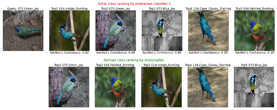
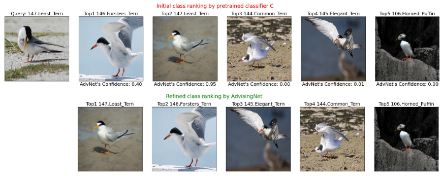
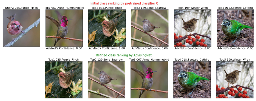
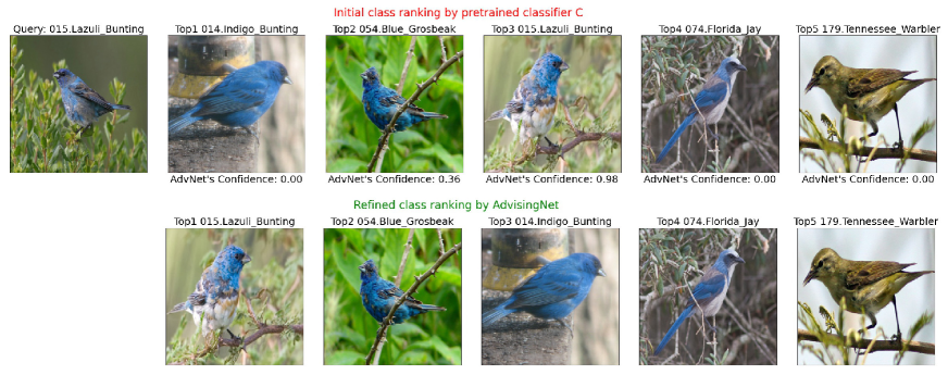
By focusing on the top-$Q$ classes as predicted by $\mathbf{C}$, this strategy mitigates issues associated with the long-tail distribution often encountered in classification problems (i.e., reducing the influence of less likely ”tail” classes). Additionally, this approach provides an added degree of interpretability since the decision-making process is based on pairwise image comparisons, allowing for an intuitive understanding of the class assignments (see Fig. 3 and Sec. A13).

3 Experimental setups

3.1 Datasets

We evaluate AdvisingNets on two datasets that have been widely utilized for benchmarking prototype-based classifiers (Chen et al. 2019; Nauta, van Bree, and Seifert 2021; Wang and Sabuncu 2022; Rymarczyk et al. 2022; Ukai et al. 2023) and explanation methods (Kim et al. 2023b, c; Morrison et al. 2023):

1. CUB-200-2011 (hereafter, CUB-200) is a collection of 11,788 images (5,994 for training and 5,794 for test) across 200 bird species;

2. Stanford Cars (hereafter, Cars-196) is a car dataset that includes 16,185 images (8,144 for training and 8,041 for test) spanning 196 distinct classes.

3.2 Pretrained classifiers $\mathbf{C}$

For CUB-200, we use a ResNet-50 model pretrained on the iNaturalist dataset and finetuned on CUB-200 (85.83% top-1 accuracy) from (Taesiri, Nguyen, and Nguyen 2022). About Cars-196, we choose three ResNet models (Eqy 2020) (i.e., ResNet-18: 86.17%, ResNet-34: 82.99%, and ResNet-50: 89.73%), all pretrained on ImageNet and finetuned on Cars-196.

3.3 Training parameters

We use Stochastic Gradient Descent (SGD) to train AdvisingNets, where convolutional layers are trainable (see Sec. A3), and adopt OneCycleLR (Smith and Topin 2019) for learning rate scheduling. Additionally, TrivialAugment (Müller and Hutter 2021) is applied to image pairs during training. This augmentation technique plays a crucial role in training AdvisingNets as it reduces overfitting (see Sec. A10). For CUB-200, we train AdvisingNets over 100 epochs with a batch size of 256 and a learning rate of $0.001$. The model architecture for this dataset is defined by $M=N=4$ and $L=2$. For Cars-196, we use the same batch size and number of epochs, but adjust the initial learning rate to $0.01$. The architecture of the model employed for this dataset is specified by $M=N=3$ and $L=3$. Unless specified differently, both the self and cross-attention Transformer blocks utilize 8 heads, and for the sampling process, $Q=K=10$. More training details are in Sec. A1.

3.4 Human-AI team set-ups

We consider multiple decision-making setups which range from human or AI model only to human-AI teams for the task of predicting whether $\mathbf{C}$ is correct or wrong:

Human only: In this setting, humans are assigned all instances to make decisions and are provided with kNN explanations (because AdvisingNets also leverage NNs).

AI auto-accept: This setting involves only the AI agent $\mathbf{C}$ and the top-1 predicted label of $\mathbf{C}$ will be automatically accepted.

AI Thresholding: Instead of automatically accepting all predictions, this setting identifies the optimal threshold on the confidence score of $\mathbf{C}$ on a validation set. In test, this threshold is used to determine whether to accept or reject decisions.

Human-Thresholding: This setup delegates uncertain predictions of $\mathbf{C}$ to humans and auto-accepts the remaining.

Human-AdvisingNet: In this setup, we replace the AI Thresholding agent with AdvisingNet. We train an AdvisingNet to align with the human-AI setup in (Taesiri, Nguyen, and Nguyen 2022) where they split the 5,794 test samples into two groups, 1,000 for validation and 4,794 for test. The validation set is used to tune the performance of both human and AI before they work complementarily on the test examples.

3.5 Baselines for image classification

We present the baseline classifiers that we use in comparisons with AdvisingNets (+ Top-classes Reranking) for multi-class image classification tasks. Please see Sec. A2 for further details and the rationale behind choosing these baseline classifiers.

Parametric classifiers (Deep CNNs): We compare against ResNet classifiers that have been trained to classify 200 Bird and 196 Car categories.

Non-parametric classifiers (kNN): kNN classifiers leverage comparisons with training prototypes to derive predicted labels. We consider kNN-RN50 and kNN-AdvNet, which uses embeddings from RN50 or AdvisingNets respectively, and select $k=20$ as in (Taesiri, Nguyen, and Nguyen 2022).

Prototypical part-based classifiers: We are interested in the comparisons with ProtoPNet (Chen et al. 2019), ProtoTree (Nauta, van Bree, and Seifert 2021), ProtoPool (Rymarczyk et al. 2022), Deformable ProtoPNet (Donnelly, Barnett, and Chen 2021), and ProtoKNN (Ukai et al. 2023).

Correspondence-based classifiers: For CUB-200, we compare against EMD-Corr and CHM-Corr (Taesiri, Nguyen, and Nguyen 2022), the two visual correspondence-based classifiers that also perform re-ranking.

4 Experimental results

We evaluate AdvisingNets on two important downstream scenarios: substituting AdvisingNet in human-AI teams and using AdvisingNet (+ TCR) to improve classifier $\mathbf{C}$ in image classification.

4.1 AdvisingNets improve human-AI team accuracy in Accepting/Rejecting AI decisions

Due to the absence of human data for Cars-196, we focus our investigation of human-AI teaming on CUB-200. As demonstrated in Table 1, AdvisingNets significantly outperforms prior baselines. When benchmarked against humans provided with nearest-neighbor explanations, AdvisingNet achieves a substantial increase in accuracy of +25.88 pts. Moreover, compared to an AI auto-accept agent, AdvisingNet improves classification performance by a margin of +4.80 pts. In the case of AI Thresholding, AdvisingNet continues to show superior performance by beating it by +3.23 pts. Against a human + AI Thresholding team, AdvisingNet showcases its strength by enhancing the classification performance by +3.97 pts.

Table 1: Binary (accept/reject) classification accuracy of various human-AI team setups on 4,794 CUB-200 test samples. ^† (Taesiri, Nguyen, and Nguyen 2022).

Classifier	Acc (%)
Human only †	64.75
AI auto-accept	85.83
AI Thresholding †	87.40
Human-Thresholding †	86.66
AdvisingNet	90.63
Human-AdvisingNet	90.65

Interestingly, we observe little improvement when comparing Human-AdvisingNet to the AdvisingNet alone. Since humans often struggle with fine-grained classification tasks (Kim et al. 2022; Colin et al. 2022; Nguyen, Kim, and Nguyen 2021), integrating humans into the team does not necessarily improve performance. Thus, in scenarios where a highly capable AI agent like the AdvisingNet is involved, human intervention may not be required in the final decision-making step. Instead, the strength of advanced AI agents might be sufficient to drive accurate outcomes.

4.2 AdvisingNets improve classifiers’ accuracy

CUB-200 image classification

Table 2: Top-1 classification accuracy of AdvisingNet and baselines on CUB-200 test set (5794 samples). We compute AdvisingNet accuracy over $3$ random seeds (see Sec. A8). ^† (Taesiri, Nguyen, and Nguyen 2022); ^♠ (Donnelly, Barnett, and Chen 2021), using full, uncropped images w/o model ensemble. ^♣ (Rymarczyk et al. 2022); ^♥ (Ukai et al. 2023), using $k=1$ like AdvisingNets and margin. All models have ResNet-50 backbone that was pretrained on i-Naturalist 2017 (Van Horn et al. 2018).

Model type	Classifier	Top-1 Acc (%)
Parametric	RN50†	85.83
Non-parametric	kNN–RN50†	85.46
	kNN–AdvNet	31.01
Prototypical part-based	ProtoPNet♠	81.10
	ProtoTree♣	82.20
	ProtoPool♣	85.50
	Def-ProtoPNet♠	86.40
	ProtoKNN♥	87.00
Correspondence-based	EMD-Corr†	84.98
	CHM-Corr†	83.27
AdvisingNet	TCR (Ours)	88.00 $\pm$ 0.11

In Table 2, AdvisingNet (+ TCR) stands out with a top-1 classification accuracy of 88.00%, directly improving RN50 by +2.17 pts. Its performance also beats the results achieved by all of non-parametric, prototypical part-based, and correspondence-based classifiers on the challenging CUB-200 test set.

Compared to a non-parametric classifier (kNN-RN50) that achieves an accuracy of 85.46%, AdvisingNet demonstrates a clear advantage in classification accuracy. The poor performance of kNN-AdvNet is because the discriminative power has been shifted to the Transformer layers. This transition causes the kNN algorithm, working on the convolutional features, to significantly reduce the accuracy compared to using the original features of RN50, from 85.46% to 31.01%. Among the prototypical part-based classifiers, namely ProtoPNet, ProtoTree, ProtoPool, Def-ProtoPNet, and ProtoKNN, AdvisingNet maintains its lead with margins ranging from 1.00 to 6.90 pts. Additionally, when compared to the correspondence-based classifiers, EMD-Corr (84.98%) and CHM-Corr (83.27%), AdvisingNet’s performance remains superior.

The improvement of the CUB-200 RN50 classifier, as presented in Table 2, can be attributed to the power of the re-ranking algorithm (TCR). We illustrate this re-ranking in Fig. 3. For example, RN50 initially incorrectly classified the query of Green Jay as Indigo Bunting. However, upon reviewing the top-predicted classes, The AdvisingNet determines that RN-50’s second-highest predicted label is a better fit for the query image, subsequently identifying Green Jay as the correct classification for the query. We provide a more comprehensive set of examples in Sec. A13.

Figure 3: An example of how AdvisingNet corrects a previously incorrect prediction on CUB-200. A RN50 model makes predictions on the Query image (ground-truth label: Green Jay) and produces initial ranking (top row) but the top-1 predicted class (Indigo Bunting) is incorrect. The AdvisingNet compares the query image with the representative of each class (the first NN example in each class) to re-rank those classes based on its confidence scores. The refined class ranking is presented in the bottom row where the Green Jay class has been successfully recognized as top-1.

Cars-196 image classification

Table 3: Top-1 classification accuracy of AdvisingNet and baselines on Stanford Cars-196 test set (8041 samples). We compute AdvisingNet accuracy over $3$ random seeds (see Sec. A8). ^† (Eqy 2020); ^♣ (Rymarczyk et al. 2022); ^♥ (Ukai et al. 2023), using $k=1$ like AdvisingNets and margin. All models started from the same ImageNet ResNet-50 backbone (Russakovsky et al. 2015).

Model type	Classifier	Top-1 Acc (%)
Parametric	RN50†	89.73
Non-parametric	kNN-RN50†	87.48
	kNN-AdvNet	16.90
Prototypical part-based	ProtoTree♣	86.60
	ProtoPool♣	88.90
	ProtoKNN♥	90.20
AdvisingNet	TCR (Ours)	90.37 $\pm$ 0.04

In Table 3, we present an analysis of top-1 classification accuracy on the Cars-196 test set. Our proposed approach, AdvisingNet (+ TCR), outperforms both the non-parametric classifier (kNN-RN50) and the parametric classifier (RN50) by +2.89 pts and +0.64 pts, respectively. We also notice a similar drop in classification accuracy when utilizing retrained convolutional features (kNN-AdvNet), as seen in CUB-200. Among the prototypical part-based classifiers, ProtoPool achieves 88.90%, ProtoTree achieves 86.60%, and ProtoKNN achieves 90.20%. Notably, our proposed approach, AdvisingNet (Top-classes Reranking), excels with a remarkable top-1 classification accuracy of 90.37%. Both AdvisingNet and ProtoKNN stand out as top-performing models in this dataset.

Model generalization tests for AdvisingNets

While we have shown that AdvisingNets (+ TCR) can improve the accuracy of pretrained models seen in training, we also wish to study their generalizability to pretrained models not seen during training (unseen models). To answer this question, we use an AdvisingNet trained on ResNet-50 (85.83% top-1 accuracy) to refine the predictions of NTS-Net (Yang et al. 2018) (87.43% top-1 accuracy) for CUB-200. For the Cars-196 dataset, we choose an AdvisingNet trained on ResNet-18 (86.17% top-1 accuracy) to improve the performance of MobileNet-V2 (87.49% top-1 accuracy).

Table 4: Top-1 classification accuracy (%) of unseen classifiers before and after working with AdvisingNets.

Dataset	Seen classifier	Unseen classifier
CUB-200	RN50	NTS-Net	Improved
	85.83	87.43	88.44 (+1.01)
Cars-196	RN18	MobileNet-V2	Improved
	86.17	87.49	87.89 (+0.40)

As summarized in Table 4, we find that AdvisingNets clearly improve the performance of unseen classifiers. The NTS-Net model, when tested on CUB-200, has been improved by +1.01 pts. Similarly, the MobileNet-V2 model on Cars-196 benefits from a +0.40 pts increase in accuracy. This is intriguing because AdvisingNets have never seen the distributions of top-predicted classes and the retrieved NNs from such out-of-training classifiers.

Additionally, we test whether AdvisingNets can boost the accuracy of pretrained classifiers beyond RN50 by training two AdvisingNets using RN34 and RN18 for Cars-196, with results detailed in Sec. A6 and  A9. Interestingly, we also achieve improvements of +1.15 pts for RN34 and +0.83 pts for RN18 in Cars classification.

Hyperparameter tests for AdvisingNets

As mentioned in Sec. 2.1, AdvisingNets learn to compare the input query with a single nearest neighbor. We expand this by averaging results from 3 or 5 pairwise comparisons in test. We find that using more NNs for comparisons marginally enhances the performance but also incurs higher computational cost (see Sec. A7 for details). Finally, our experiments opt for empirical settings with $Q=K=10$. We delve into different values of $Q$ and $K$ in Sec. A11. Although smaller values considerably diminish AdvisingNet’s performance, we observe a slight improvement in accuracy when increasing these values from 10 to 15.

5 Related Works

Learning from nearest-neighbor-based positive and negative pairs.

Contrastive learning is a self-supervised learning technique that aims to maximize the agreement between positive pairs and minimize it between negative pairs to learn more meaningful representations. Nearest neighbors have emerged as a key component in the sample selection step of contrastive learning pipelines (Dwibedi et al. 2021; Mou et al. 2022; Liu et al. 2023; Chongjian et al. 2022).

While training Advisingnets also utilizes positive and negative instances as in contrastive learning approaches, our training pipeline differs in that we leverage the top-predicted labels of a pretrained model to determine the classes for sampling. Moreover, while existing works typically optimize for contrastive loss functions like InfoNCE (Oord, Li, and Vinyals 2018), we directly train a binary classification model using cross entropy loss, which simplifies the training process.

Effective AI agents for human-AI teaming.

One of the applications studied in this work is human-AI teaming, which refers to setups where humans and AI agents work together to make better and more responsible decisions than either could achieve solo. In many setups, AI agents support humans who are the final decision-makers (Bansal et al. 2021) or they might simply rely on model uncertainty (Taesiri, Nguyen, and Nguyen 2022) in decision-making, leading to reduced human-AI performance and potential fragility in OOD environments where models exhibit high confidence but make erroneous predictions (Nguyen, Yosinski, and Clune 2015). In response to these challenges, we introduce AdvisingNet, an effective AI agent designed to make decisions by considering both the input image and external knowledge sources (i.e., training nearest neighbors).

Ranking-based image classification.

A second task studied in this work is the use of AdvisingNet to improve a pretrained image classifier. In general, image classification models are typically softmax-based classifiers, which rank all potential classes using logit scores and designate the highest-scoring class as the predicted label for a given image. In contrast, ProtoPNet (Chen et al. 2019), an interpretable model that classifies images by matching parts of the input image to patch prototypes found in the training set, determines the class rankings via the similarity between the input features and those of each class. This strategy is also found in k-nearest neighbors (kNN) algorithms, where the nearest neighbors are ranked based on the similarity to the input image (Papernot and McDaniel 2018).

There have recently been proposals for re-ranking the neighbor candidates retrieved from kNN classifiers to refine the initial predictions using both image-level and patch-wise comparisons (Phan and Nguyen 2022; Taesiri, Nguyen, and Nguyen 2022). Rather than refining predictions by re-ranking nearest neighbors from kNN classifiers, we steer our attention towards optimizing the ranking of top-predicted classes resulting from a softmax classifier. Furthermore, while traditional kNN-based strategies and methods like ProtoPNet (Chen et al. 2019) require significant computational resources due to the need for pairwise distance calculations or examination of all classes, our proposed algorithm TCR alleviates this demand by focusing only on a few top-predicted classes, concentrating computational resources in the most promising regions of the classification space. Put simply, the ranking is based not on similarity scores but on the confidences of AdvisingNet for classes.

6 Conclusion

We present AdvisingNet, a model that compares an input image against its nearest neighbors to effectively classify whether a pretrained model correctly classifies an input image. In general, we found that AdvisingNets significantly outperformed previous human, AI, and team baselines in the task of classifying correct and incorrect predictions. Additionally, while AdvisingNets were not explicitly trained for multi-class image classification tasks, we also observed that they consistently help achieve accuracy that either outperformed or was on par with, state-of-the-art methods on both the CUB-200 and Cars-196 datasets. The benefits of using AdvisingNets over traditional deep CNN classifiers indicate the benefits of leveraging external data, especially nearest neighbors, to help in fine-grained classification tasks.

Future Work and Limitations.

Our findings suggest that AdvisingNets are not limited to improving only ResNets, but extend to enhancing any classification models. In cases where it is not feasible to leverage convolutional features as image-representing patch tokens, we can patchify images and encode them in a similar fashion as Vision Transformers (ViT) (Dosovitskiy et al. 2020).

Due to computational constraints, scaling AdvisingNets for large-scale classification datasets, such as ImageNet (Russakovsky et al. 2015), has not been explored in this work. We also anticipate a connection between the performance of AdvisingNets and that of the pretrained models, a relationship that has not been investigated yet.

Appendix A1 More training details of AdvisingNets

For training AdvisingNets, the F1 score was chosen as the evaluation metric to select the optimal AdvisingNets for testing (because we are training binary classifiers). Our experiments were conducted using two NVIDIA A100-SXM4-40GB GPUs, leveraging PyTorch version 1.13.0+cu117. Unless mentioned otherwise, a consistent seed value of 42 was set to ensure reproducibility across Python, Numpy, and PyTorch operations. We employ the faiss (Johnson, Douze, and Jégou 2019) library to index and retrieve nearest neighbors, utilizing the Euclidean distance through the IndexFlatL2 function.

Appendix A2 Details of baseline image classifiers

A2.1 Non-parametric classifiers (kNNs)

Both AdvisingNets and kNN classifiers leverage the comparison between a test image and training samples to derive a prediction. However, they differ in how they perform the comparison. While kNN classifiers use global nearest neighbors, AdvisingNets localize the search regions (classes of interest) by comparing the input with nearest neighbors only from the top-predicted classes of a classifier $\mathbf{C}$. We propose to compare with kNN-RN50 and kNN-AdvNet (where $k=20$ as in (Taesiri, Nguyen, and Nguyen 2022)). Both these classifiers operate on conv4 features and use cosine distance to rank NNs. While kNN-RN50 is based on the pretrained $\mathbf{C}$’s conv features, kNN-AdvNet uses the retrained conv features of AdvisingNets.

A2.2 Parametric classifiers (Deep convolution neural networks – CNNs)

While softmax-based classifiers are powerful, they only use the input image only and lack the capability of providing explanations. In contrast, AdvisingNets utilize nearest neighbors to enhance the interpretability and performance of a pretrained model without retraining it. However, one downside of AdvisingNets compared to softmax-based classifiers is the computational overhead due to the extra Transformer layers used for image comparison. We compare our method with ResNet-50 (RN50) classifiers that have been trained to classify 200 Bird and 196 Car categories.

A2.3 Prototypical part-based classifiers

Both AdvisingNets and prototypical part-based classifiers use patch-level representations to compare the input with training examples and produce similarity scores (i.e., equivalent to the logit scores produced by AdvisingNets). However, while AdvisingNets focus on examining a small set of classes, ProtoPNet (Chen et al. 2019) and its siblings consider all possible classes. Furthermore, AdvisingNets allow for knowledge expansion without retraining the model (i.e., we can extend the database for nearest neighbor retrieval), highlighting its flexibility in accommodating additional information outside the training set. We are interested in the comparisons with ProtoPNet (Chen et al. 2019), ProtoTree (Nauta, van Bree, and Seifert 2021), ProtoPool (Rymarczyk et al. 2022), Deformable ProtoPNet (Donnelly, Barnett, and Chen 2021), and ProtoKNN (Ukai et al. 2023).

A2.4 Correspondence-based classifiers

These image classifiers leverage the correspondences between the input image and training examples to re-rank the results of kNN retrieval, thereby redoing the majority vote (Phan and Nguyen 2022; Taesiri, Nguyen, and Nguyen 2022). Meanwhile, our AdvisingNets use Algorithm 1 (Top-classes Reranking) to re-rank the top-predicted classes of a classifier $\mathbf{C}$. This difference is compelling, as the ground-truth label is more likely to be in the top-predicted classes of $\mathbf{C}$. We take EMD-Corr and CHM-Corr (Taesiri, Nguyen, and Nguyen 2022), the two visual correspondence-based classifiers, into comparisons for CUB-200 and report in Table 2.

Appendix A3 Do we need to retrain conv layers of classifiers $\mathbf{C}$?

In the training process of AdvisingNets, one crucial consideration is whether to retrain the conv layers from the pretrained models. If these layers are already generating effective encodings for the binary classification task, then we should focus on optimizing the remaining layers. To evaluate the effects of retraining the conv layers, we conduct an experiment involving the training of an AdvisingNet for CUB-200 using the ResNet-50 backbone. In this experiment, we freeze the conv layers while maintaining other settings as the same. The result of this experiment is that freezing the conv layers significantly slows down the learning process of the AdvisingNet. Specifically, the model could only reach its peak training accuracy of 94.18% after 100 epochs and test accuracy of 87.56% (lower than 90.20% when making conv layers trainable in Table A3).

Appendix A4 Human-AI teaming setup with AdvisingNets

We follow the experimental setup for human-AI collaboration from (Taesiri, Nguyen, and Nguyen 2022), where humans and AIs work collaboratively to accept and reject a pretrained ResNet-50’s predictions. We train an AdvisingNet using an iNaturalist-pretrained ResNet-50 with 5,994 training samples from CUB-200. Similar to (Taesiri, Nguyen, and Nguyen 2022), we split the 5,794 test samples into two groups, 1,000 for validation and 4,794 for testing. We describe next how we use the validation set to tune the performance of both human and AI before they work complementarily on the test examples.

Figure F1: Human-AI interaction model with AdvisingNet. Samples that the AI (pretrained ResNet-50) classifies with high confidence are delegated to the AdvisingNet, while the remaining images are routed to humans.

Following the interaction model 2 presented by (Taesiri, Nguyen, and Nguyen 2022), we incorporate the AdvisingNet into the decision-making process alongside human users (see Fig. F1). We substitute the Thresholding agent with the AdvisingNet and enable the collaboration at a confidence threshold T of 90% – a level determined as optimal from 1,000 validation samples. Rather than the AI making all final decisions, it only addresses inputs $\mathbf{C}$ deems most confident in. Consequently, human users are tasked with labeling the more challenging cases. Essentially, this approach substitutes the naive AI agent, referred to as Thresholding, by the AdvisingNet.

Appendix A5 Sanity checks for AdvisingNets via controlling explanations

In this section, we investigate the logical consistency of AdvisingNets. Specifically, we evaluate the model’s ability to correctly distinguish images that are the same and different. This is achieved by comparing AdvisingNets’ responses when the NN is the input query itself (expected output: 1 or Yes) and when the NN is a randomly sampled image (expected output: 0 or No). When sampling the random NN, we study two scenarios: one where NNs are assigned random values and another where they are random real images. These random real images are sampled by shuffling the NNs in image pairs inside a batch size of 11 pairs.

Table A1: The sanity checks for AdvisingNets.

Dataset	Explanation	Yes Ratio (%)
CUB-200	Query	100
	Random values	3.52
	Random real images	8.63
Cars-196	Query	100
	Random values	2.05
	Random real images	8.61

As seen in Table A1, when the NN provided is the input image, AdvisingNets correctly recognize the two images as being from the same class, yielding a Yes ratio of 100%. On the other hand, when a random-valued NN is used, the AdvisingNets correctly identify that the images are not from the same class, yielding low Yes ratios, namely 3.52% and 2.05% for CUB-200 and Cars-196 datasets, respectively. The ratios represented by Yes for random-real images are also low for both datasets, as expected. This verifies the logical consistency of AdvisingNets.

Appendix A6 Generalization tests of for the TCR algorithm

To study the generalization of TCR on different pretrained classifiers, we conduct experiments using RN18 and RN34 on Cars-196 dataset, outlined in Table A2. After training AdvisingNets and integrating them with the pretrained models (i.e., via the TCR algorithm), we observe consistent improvements, +1.15 pts for RN34 and +0.83 pts for RN18.

Table A2: AdvisingNets consistently improve pretrained models across architectures. The accuracy is reported on the Stanford Cars-196 test set (8041 samples).

Model	Top-1 Acc (%)	TCR Top-1 Acc (%)
RN34	82.99	84.14 (+1.15)
RN18	86.17	87.00 (+0.83)

Appendix A7 Using more nearest neighbors in AdvisingNets

In this section, our aim is to examine the impact of incorporating more nearest neighbors in the binary classification task. During training, the AdvisingNets were designed to compare the input query against a single nearest neighbor. During the testing phase, we repeat this process with 3 and 5 pair-wise comparisons (i.e., pairing the input image with each of 3 or 5 nearest neighbors from each class), and subsequently take the average to render the final prediction for binary classification. The goal is to investigate whether an increase in the number of comparisons enhances the accuracy of AdvisingNets. The evaluation involves two distinct AdvisingNets, both of which were trained using the ResNet-50 architecture for CUB-200 and Cars-196.

Table A3: Accuracy (%) comparison of AdvisingNets using varying numbers of nearest neighbors for the binary classification task.

#NNs	Phase	CUB-200	Cars-196
1	Train	98.69	99.01
	Test	90.20	91.92
3	Test	90.49	92.00
5	Test	90.70	92.02

As seen in Table A3, increasing the number of nearest neighbors for comparison slightly improves the performance. With 3 nearest neighbors, the accuracy on the test set increases to 90.49% for CUB-200 and 92.00% for Cars-196. When using 5 nearest neighbors, the test accuracy increases further to 90.70% for CUB-200 and 92.02% for Cars-196. This says that incorporating more nearest neighbors in the classification task slightly enhances the performance of the AdvisingNets. However, it is noteworthy to consider the associated computational cost. The computational demands increase linearly with the number of nearest neighbors. As such, a careful balance between accuracy improvement and computational efficiency must be struck when deciding on the number of nearest neighbors to incorporate into the AdvisingNets.

Appendix A8 Training AdvisingNets with different seeds

To guarantee the improvements shown in Table 2 and  3 are statistically significant, we train those AdvisingNets multiple times with different seeds. We present the results in Table A4.

Table A4: Significance tests for AdvisingNets on CUB-200.

Run #	Train Acc (%)		Test Acc (%)		TCR Top-1 Acc (%)
	CUB-200	Cars-196	CUB-200	Cars-196	CUB-200	Cars-196
1	98.69	99.01	90.20	91.92	87.97	90.27
2	98.66	98.99	90.47	92.02	87.94	90.40
3	98.61	99.02	90.51	92.10	88.16	90.44
$\mu\pm\sigma$	98.65 $\pm$ 0.04	99.00 $\pm$ 0.02	90.39 $\pm$ 0.16	92.01 $\pm$ 0.09	88.00 $\pm$ 0.11	90.37 $\pm$ 0.04

We observe that AdvisingNets consistently achieve test accuracies for both binary and multi-way classifications across different runs. Also, we note that AdvisingNets misclassify between 8-10% of $\mathbf{C}$’s predictions (i.e., test accuracy is from 90% - 92%). Typically, the errors are primarily due to inter-class and intra-class variations, as well as issues with dataset annotations (details in Sec. A14).

Appendix A9 Changing backbones for AdvisingNets

We aim to investigate how the selection of $\mathbf{C}$ impacts the performance of AdvisingNets. Specifically, we train three distinct AdvisingNets using RN18, RN34, and RN50 on Cars-196. The term “Top-1 Acc” represents the top-1 accuracy achieved by the respective pretrained model $\mathbf{C}$. In addition, “Train Acc” denotes the accuracy of AdvisingNets on the training set, while ’Test Acc’ indicates the accuracy on the test set.

Table A5: Comparison of AdvisingNet performance using different pretrained models.

Pretrained Model	Top-1 Acc (%)	Train Acc (%)	Test Acc (%)
RN34	82.99	98.11	88.73
RN18	86.17	98.07	89.85
RN50	89.73	99.01	91.92

Based on Table A5, we see that the selection of $\mathbf{C}$ for AdvisingNets significantly influences their binary classification performance. In particular, the performance of AdvisingNets appears to be positively correlated with the capability of the underlying pretrained classifier $\mathbf{C}$. This is an expected outcome as the convolutional layers from these pretrained models are employed by the AdvisingNets for image encoding. The more powerful these layers are at extracting image features, the better the AdvisingNets perform.

Appendix A10 The effects of data augmentation

We aim to examine the impact of data augmentation on the performance of AdvisingNets by repeating our previous experiments for CUB-200 and Cars-196 datasets without applying TrivialAugment (Müller and Hutter 2021) to input and NN images. In Table A6, we observe that the model not only converges more quickly without augmentation but also attains a higher accuracy rate in the training set (i.e., 99.81% vs. 98.69% for CUB-200 and 99.79% vs. 99.01% for Cars-196).

Table A6: Accuracy (%) of AdvisingNets on CUB-200 and Cars-196 without Trivial Augmentation in training. The backbone for both models is ResNet-50. w and w/o denote using and not using Trivial Augmentation.

Phase	CUB-200		Cars-196
	w	w/o	w	w/o
Train	98.69	99.81	99.01	99.79
Test	90.20	88.61	91.92	90.19

However, the absence of data augmentation has a different effect on the test sets. While the use of data augmentation contributes to achieving an accuracy rate of 90.20%, as shown in Table A3, the omission of this technique only yields a rate of 88.61% for CUB-200. Similarly, we observe a drop in test accuracy for Cars-196 without using the data augmentation technique, from 91.92% to 90.19%. These findings underscore the importance of data augmentation in the training phase of AdvisingNets as it helps reduce overfitting.

Appendix A11 The effects of $Q$ and $K$ in sample selection to AdvisingNet’s performance

$Q$ and $K$ are crucial hyperparameters for training AdvisingNets. To examine their effects, beyond the default setting of $Q=K=10$, we also train AdvisingNets with configurations of $Q=K=3$, $5$, and $15$. By default, Q is set equal to K, and these values represent the coverage of the sampling process over the nearest neighbor space.

However, large values can also introduce noise during training. This is because NNs from the tails of the top-1 class (as depicted by the last images in the middle row of Fig. 2(a)) and predicted classes (shown by the last images in the bottom row of Fig. 2(a)) are trivial and might not help AdvisingNets much in classifying top-1 predicted labels.

Table A7: The accuracy of AdvisingNets trained on different values of Q (K) for CUB-200.

Q	K	Train Acc (%)	Test Acc (%)
3		97.17	87.81
5		97.60	89.56
10		98.69	90.20
15		99.30	90.56

From Table A7, we note that these values significantly influence the performance of AdvisingNets. Interestingly, there appears to be a trend: as these values increase (indicating more training data), the test accuracy also improves. However, there is a balance to strike between test accuracy and computational demand. As per Table A7, 10 emerges as an optimal choice for CUB-200.

Appendix A12 Showcasing nearest neighbors for training

We show the nearest neighbors utilized for forming training pairs in training AdvisingNets in Figs. F2,  F3 for CUB-200 and Fig. F4,  F5 for Cars-196. From the top-1 predicted classes, we assemble $K$ pairs. For the remaining classes beyond the top-1, we fetch the first nearest neighbor within each class and combine with the respective query sample. With $Q=K=10$, a total of 19 pairs are formulated.

When we prompt the pretrained model $\mathbf{C}$ to make predictions on its training data $x$, it is reasonable to expect the top-1 predicted class to match the ground-truth label. This expectation is grounded in the fact that model $\mathbf{C}$ typically exhibits nearly perfect accuracy (around 100%) on its training set.

(a)

(b)

Figure F2: Training pairs for CUB-200 AdvisingNets. For a given query, a pretrained model $\mathbf{C}$ predicts the label Field Sparrow (a) and Pied Billed Grebe (b), which align with the ground-truth labels. Subsequently, from each of these query images, we generate 10 positive pairs (using NNs of top-1 class in the middle row) and 9 negative pairs (using NNs of top-2 to 10 classes in the bottom row).

(a)

(b)

Figure F3: Training pairs for CUB-200 AdvisingNets. For a given query, a pretrained model $\mathbf{C}$ predicts the label Chipping Sparrow (a) and California Gull (b), which align with the ground-truth labels. Subsequently, from each of these query images, we generate 10 positive pairs (using NNs of top-1 class in the middle row) and 9 negative pairs (using NNs of top-2 to 10 classes in the bottom row).

(a)

(b)

Figure F4: Training pairs for Cars-196 AdvisingNets. For a given query, a pretrained model $\mathbf{C}$ predicts the label Suzuki SX4 Hatchback 2012 (a) and Hyundai Azera Sedan 2012 (b), which match the ground-truth labels. Subsequently, from each of these query images, we generate 10 positive pairs (using NNs of top-1 class in the middle row) and 9 negative pairs (using NNs of top-2 to 10 classes in the bottom row).

(a)

(b)

Figure F5: Training pairs for Cars-196 AdvisingNets. For a given query, a pretrained model $\mathbf{C}$ predicts the label Ford Freestar Minivan 2007 (a) and Dodge Caravan Minivan 1997 (b), which match the ground-truth labels. Subsequently, from each of these query images, we generate 10 positive pairs (using NNs of top-1 class in the middle row) and 9 negative pairs (using NNs of top-2 to 10 classes in the bottom row).

Appendix A13 AdvisingNets correct top-1 mispredictions of pretrained classifiers

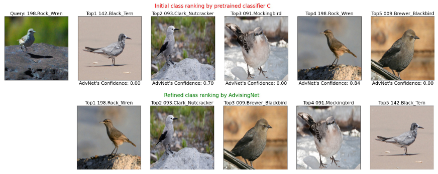
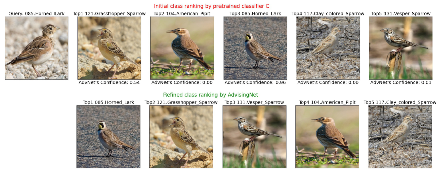
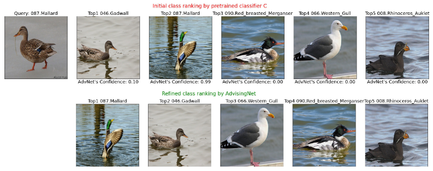
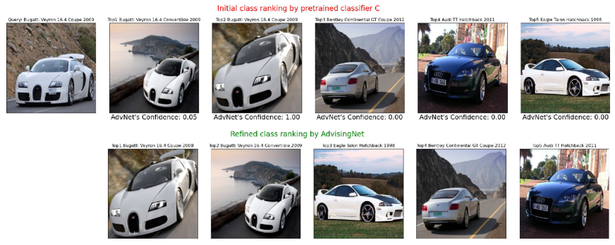
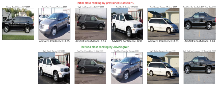
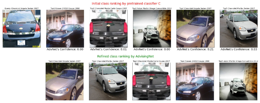
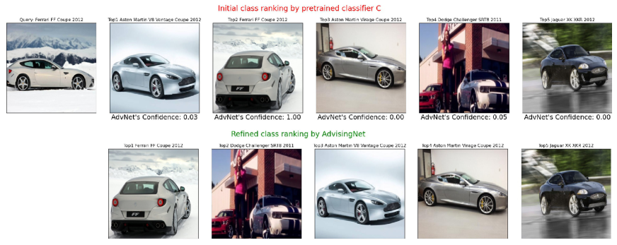
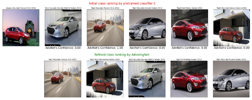
We present cases where AdvisingNets correct the top-1 predictions made by pretrained classifiers $\mathbf{C}$ on CUB-200 (Figs F7, F7, F9, F9, F11, F11) and Cars-196 (Figs F13, F13, F15, F15, F17, F17).

Figure F6: The correction of an AdvisingNet trained on CUB-200. A pretrained model $\mathbf{C}$ makes predictions on the Query image (ground-truth label: Least Tern) and produces initial ranking (top row) but the top-1 predicted class (Forsters Tern) does not match the ground-truth label. The AdvisingNet compares the query image with the representative of each class (the first NN example in each class) to re-rank those classes based on confidence scores. The refined class ranking is presented in the bottom row where the Least Tern class has been recognized as top-1.

Figure F7: A pretrained model $\mathbf{C}$ makes predictions on the Query image (ground-truth label: Purple Finch) and produces initial ranking (top row) but the top-1 predicted class (Anna Hummingbird) does not match the ground-truth label. The refined class ranking is presented in the bottom row where the Purple Finch class has been recognized as top-1.

Figure F8: A pretrained model $\mathbf{C}$ makes predictions on the Query image (ground-truth label: Lazuli Bunting) and produces initial ranking (top row) but the top-1 predicted class (Indigo Bunting) does not match the ground-truth label. The refined class ranking is presented in the bottom row where the Lazuli Bunting class has been recognized as top-1.

Figure F9: A pretrained model $\mathbf{C}$ makes predictions on the Query image (ground-truth label: Rock Wren) and produces initial ranking (top row) but the top-1 predicted class (Black Tern) does not match the ground-truth label. The refined class ranking is presented in the bottom row where the Rock Wren class has been recognized as top-1.

Figure F10: A pretrained model $\mathbf{C}$ makes predictions on the Query image (ground-truth label: Horned Lark) and produces initial ranking (top row) but the top-1 predicted class (Grasshopper Sparrow) does not match the ground-truth label. The refined class ranking is presented in the bottom row where the Horned Lark class has been recognized as top-1.

Figure F11: A pretrained model $\mathbf{C}$ makes predictions on the Query image (ground-truth label: Mallard) and produces initial ranking (top row) but the top-1 predicted class (Gadwall) does not match the ground-truth label. The refined class ranking is presented in the bottom row where the Mallard class has been recognized as top-1.

Figure F12: The correction of an AdvisingNet trained on Cars-196. A pretrained model $\mathbf{C}$ makes predictions on the Query image (ground-truth label: Bugatti Veyron 16.4 Coupe 2009) and produces initial ranking (top row) but the top-1 predicted class does not match the ground-truth label. The AdvisingNet compares the query image with the representative of each class (the first NN example in each class) to re-rank those classes based on confidence scores. The refined class ranking is presented in the bottom row where the Bugatti Veyron 16.4 Coupe 2009 class has been recognized as top-1.

Figure F13: A pretrained model $\mathbf{C}$ makes predictions on the Query image (ground-truth label: Buick Rainier SUV 2007) and produces initial ranking (top row) but the top-1 predicted class does not match the ground-truth label. The refined class ranking is presented in the bottom row where the Buick Rainier SUV 2007 class has been recognized as top-1.

Figure F14: A pretrained model $\mathbf{C}$ makes predictions on the Query image (ground-truth label: Chevrolet Impala Sedan 2007) and produces initial ranking (top row) but the top-1 predicted class does not match the ground-truth label. The refined class ranking is presented in the bottom row where the Chevrolet Impala Sedan 2007 class has been recognized as top-1.

Figure F15: A pretrained model $\mathbf{C}$ makes predictions on the Query image (ground-truth label: Ferrari FF Coupe 2012) and produces initial ranking (top row) but the top-1 predicted class does not match the ground-truth label. The refined class ranking is presented in the bottom row where the Ferrari FF Coupe 2012 class has been recognized as top-1.

Figure F16: A pretrained model $\mathbf{C}$ makes predictions on the Query image (ground-truth label: Hyundai Tucson SUV 2012) and produces initial ranking (top row) but the top-1 predicted class does not match the ground-truth label. The refined class ranking is presented in the bottom row where the Hyundai Tucson SUV 2012 class has been recognized as top-1.

Figure F17: A pretrained model $\mathbf{C}$ makes predictions on the Query image (ground-truth label: Spyker C8 Coupe 2009) and produces initial ranking (top row) but the top-1 predicted class does not match the ground-truth label. The refined class ranking is presented in the bottom row where the Spyker C8 Coupe 2009 class has been recognized as top-1.

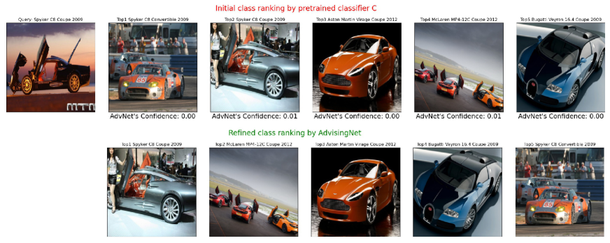
Appendix A14 An analysis of AdvisingNets’ failures

The classification performance of AdvisingNets on $\mathbf{C}$’s correct/incorrect predictions varies from 90% to 92% for both datasets. We are keen to investigate the cases where AdvisingNets does not perform accurately to better understand the limitations of them.

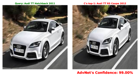
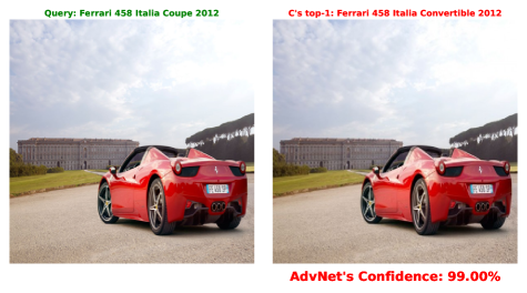
We find that if AdvisingNets incorrectly predict that two images are from the same class, the image pairs often indeed appear to be very similar. Through this analysis, we were able to find multiple examples of two identical images which had two different labels (i.e., wrong annotations in Cars-196).

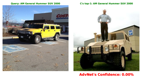
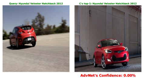
In contrast, when AdvisingNets incorrectly predict that two images are dissimilar, the image pairs display notable differences (e.g., due to different lighting or angles). Qualitative results can be found in Fig. F18 for CUB-200 and Fig. F19 for Cars-196.

(a)

(b)

Figure F18: Failures of an AdvisingNet (90.20% test acc) on CUB-200. (a) AdvisingNet incorrectly accepted the $\mathbf{C}$’s predictions for both images. For the left image, the two birds (Swainson Warbler vs. Carolina Wren) appear similar. For the right image, the birds (Black Tern vs. Least Tern) also appear visually similar. Both scenarios led AdvisingNet to accept with high confidence. (b) AdvisingNet incorrectly rejected the $\mathbf{C}$’s predictions for both images. For the left image, the bird is a Pied Kingfisher. For the right image, the bird is a Elegant Tern. Both sets of birds show variations, leading AdvisingNet to mistakenly reject the prediction.

(a)

(b)

Figure F19: Failures of an AdvisingNet (91.92% test acc) on Cars-196. (a) AdvisingNet incorrectly accepted the $\mathbf{C}$’s predictions for both images. We discovered that the cars are indeed identical. The AdvisingNet’s misclassifications are due to errors in the Cars-196 dataset annotations. (b) AdvisingNet incorrectly rejected the $\mathbf{C}$’s predictions for both images. We observed that, in most instances, the cars display noticeable differences, such as color, viewing angle, and lighting.

References

- Bansal et al. (2021) Bansal, G.; Wu, T.; Zhou, J.; Fok, R.; Nushi, B.; Kamar, E.; Ribeiro, M. T.; and Weld, D. 2021. Does the whole exceed its parts? the effect of ai explanations on complementary team performance. In Proceedings of the 2021 CHI Conference on Human Factors in Computing Systems, 1–16.
- Chen et al. (2023a) Chen, C.; Feng, S.; Sharma, A.; and Tan, C. 2023a. Machine Explanations and Human Understanding. In Proceedings of the 2023 ACM Conference on Fairness, Accountability, and Transparency, 1–1.
- Chen et al. (2019) Chen, C.; Li, O.; Tao, D.; Barnett, A.; Rudin, C.; and Su, J. K. 2019. This looks like that: deep learning for interpretable image recognition. Advances in neural information processing systems, 32.
- Chen, Fan, and Panda (2021) Chen, C.-F. R.; Fan, Q.; and Panda, R. 2021. Crossvit: Cross-attention multi-scale vision transformer for image classification. In Proceedings of the IEEE/CVF international conference on computer vision, 357–366.
- Chen et al. (2023b) Chen, V.; Liao, Q. V.; Vaughan, J. W.; and Bansal, G. 2023b. Understanding the role of human intuition on reliance in human-AI decision-making with explanations. arXiv preprint arXiv:2301.07255.
- Chongjian et al. (2022) Chongjian, G.; Wang, J.; Tong, Z.; Chen, S.; Song, Y.; and Luo, P. 2022. Soft Neighbors are Positive Supporters in Contrastive Visual Representation Learning. In The Eleventh International Conference on Learning Representations.
- Colin et al. (2022) Colin, J.; Fel, T.; Cadène, R.; and Serre, T. 2022. What i cannot predict, i do not understand: A human-centered evaluation framework for explainability methods. Advances in Neural Information Processing Systems, 35: 2832–2845.
- Donnelly, Barnett, and Chen (2021) Donnelly, J.; Barnett, A. J.; and Chen, C. 2021. Deformable ProtoPNet: An Interpretable Image Classifier Using Deformable Prototypes. arXiv preprint arXiv:2111.15000.
- Dosovitskiy et al. (2020) Dosovitskiy, A.; Beyer, L.; Kolesnikov, A.; Weissenborn, D.; Zhai, X.; Unterthiner, T.; Dehghani, M.; Minderer, M.; Heigold, G.; Gelly, S.; et al. 2020. An image is worth 16x16 words: Transformers for image recognition at scale. arXiv preprint arXiv:2010.11929.
- Dwibedi et al. (2021) Dwibedi, D.; Aytar, Y.; Tompson, J.; Sermanet, P.; and Zisserman, A. 2021. With a little help from my friends: Nearest-neighbor contrastive learning of visual representations. In Proceedings of the IEEE/CVF International Conference on Computer Vision, 9588–9597.
- Eqy (2020) Eqy. 2020. PyTorch-Stanford-Cars-Baselines. https://github.com/eqy/PyTorch-Stanford-Cars-Baselines.git.
- Jin, Li, and Hamarneh (2021) Jin, W.; Li, X.; and Hamarneh, G. 2021. One map does not fit all: Evaluating saliency map explanation on multi-modal medical images. arXiv preprint arXiv:2107.05047.
- Jin, Li, and Hamarneh (2022) Jin, W.; Li, X.; and Hamarneh, G. 2022. Evaluating explainable AI on a multi-modal medical imaging task: Can existing algorithms fulfill clinical requirements? In Proceedings of the AAAI Conference on Artificial Intelligence, volume 36, 11945–11953.
- Johnson, Douze, and Jégou (2019) Johnson, J.; Douze, M.; and Jégou, H. 2019. Billion-scale similarity search with GPUs. IEEE Transactions on Big Data, 7(3): 535–547.
- Kim et al. (2023a) Kim, J. S.; Chen, V.; Pruthi, D.; Shah, N. B.; and Talwalkar, A. 2023a. Assisting Human Decisions in Document Matching. arXiv preprint arXiv:2302.08450.
- Kim et al. (2022) Kim, S. S.; Meister, N.; Ramaswamy, V. V.; Fong, R.; and Russakovsky, O. 2022. Hive: evaluating the human interpretability of visual explanations. In Computer Vision–ECCV 2022: 17th European Conference, Tel Aviv, Israel, October 23–27, 2022, Proceedings, Part XII, 280–298. Springer.
- Kim et al. (2023b) Kim, S. S.; Watkins, E. A.; Russakovsky, O.; Fong, R.; and Monroy-Hernández, A. 2023b. ” Help Me Help the AI”: Understanding How Explainability Can Support Human-AI Interaction. In Proceedings of the 2023 CHI Conference on Human Factors in Computing Systems, 1–17.
- Kim et al. (2023c) Kim, S. S.; Watkins, E. A.; Russakovsky, O.; Fong, R.; and Monroy-Hernández, A. 2023c. Humans, AI, and Context: Understanding End-Users’ Trust in a Real-World Computer Vision Application. In Proceedings of the 2023 ACM Conference on Fairness, Accountability, and Transparency, 77–88.
- Krause et al. (2013) Krause, J.; Stark, M.; Deng, J.; and Fei-Fei, L. 2013. 3d object representations for fine-grained categorization. In Proceedings of the IEEE international conference on computer vision workshops, 554–561.
- Liu et al. (2022) Liu, H.; Tian, Y.; Chen, C.; Feng, S.; Chen, Y.; and Tan, C. 2022. Learning Human-Compatible Representations for Case-Based Decision Support. In The Eleventh International Conference on Learning Representations.
- Liu et al. (2023) Liu, Y.; Wang, Y.; Chen, Y.; Dai, W.; Li, C.; Zou, J.; and Xiong, H. 2023. Promoting Semantic Connectivity: Dual Nearest Neighbors Contrastive Learning for Unsupervised Domain Generalization. In Proceedings of the IEEE/CVF Conference on Computer Vision and Pattern Recognition, 3510–3519.
- Morrison et al. (2023) Morrison, K.; Spitzer, P.; Turri, V.; Feng, M.; Kühl, N.; and Perer, A. 2023. The Impact of Imperfect XAI on Human-AI Decision-Making. arXiv:2307.13566.
- Mou et al. (2022) Mou, Y.; He, K.; Wang, P.; Wu, Y.; Wang, J.; Wu, W.; and Xu, W. 2022. Watch the Neighbors: A Unified K-Nearest Neighbor Contrastive Learning Framework for OOD Intent Discovery. In Proceedings of the 2022 Conference on Empirical Methods in Natural Language Processing, 1517–1529.
- Müller and Hutter (2021) Müller, S. G.; and Hutter, F. 2021. Trivialaugment: Tuning-free yet state-of-the-art data augmentation. In Proceedings of the IEEE/CVF international conference on computer vision, 774–782.
- Nauta, van Bree, and Seifert (2021) Nauta, M.; van Bree, R.; and Seifert, C. 2021. Neural prototype trees for interpretable fine-grained image recognition. In Proceedings of the IEEE/CVF Conference on Computer Vision and Pattern Recognition, 14933–14943.
- Nguyen, Yosinski, and Clune (2015) Nguyen, A.; Yosinski, J.; and Clune, J. 2015. Deep neural networks are easily fooled: High confidence predictions for unrecognizable images. In Proceedings of the IEEE conference on computer vision and pattern recognition, 427–436.
- Nguyen, Kim, and Nguyen (2021) Nguyen, G.; Kim, D.; and Nguyen, A. 2021. The effectiveness of feature attribution methods and its correlation with automatic evaluation scores. Advances in Neural Information Processing Systems, 34: 26422–26436.
- Oord, Li, and Vinyals (2018) Oord, A. v. d.; Li, Y.; and Vinyals, O. 2018. Representation learning with contrastive predictive coding. arXiv preprint arXiv:1807.03748.
- Papernot and McDaniel (2018) Papernot, N.; and McDaniel, P. 2018. Deep k-nearest neighbors: Towards confident, interpretable and robust deep learning. arXiv preprint arXiv:1803.04765.
- Phan and Nguyen (2022) Phan, H.; and Nguyen, A. 2022. DeepFace-EMD: Re-ranking using patch-wise earth mover’s distance improves out-of-distribution face identification. In Proceedings of the IEEE/CVF Conference on Computer Vision and Pattern Recognition, 20259–20269.
- Russakovsky et al. (2015) Russakovsky, O.; Deng, J.; Su, H.; Krause, J.; Satheesh, S.; Ma, S.; Huang, Z.; Karpathy, A.; Khosla, A.; Bernstein, M.; et al. 2015. Imagenet large scale visual recognition challenge. International Journal of Computer Vision, 115(3): 211–252.
- Rymarczyk et al. (2022) Rymarczyk, D.; Struski, Ł.; Górszczak, M.; Lewandowska, K.; Tabor, J.; and Zieliński, B. 2022. Interpretable image classification with differentiable prototypes assignment. In European Conference on Computer Vision, 351–368. Springer.
- Smith and Topin (2019) Smith, L. N.; and Topin, N. 2019. Super-convergence: Very fast training of neural networks using large learning rates. In Artificial intelligence and machine learning for multi-domain operations applications, volume 11006, 369–386. SPIE.
- Taesiri et al. (2023) Taesiri, M. R.; Nguyen, G.; Habchi, S.; Bezemer, C.-P.; and Nguyen, A. 2023. Zoom is what you need: An empirical study of the power of zoom and spatial biases in image classification. arXiv preprint arXiv:2304.05538.
- Taesiri, Nguyen, and Nguyen (2022) Taesiri, M. R.; Nguyen, G.; and Nguyen, A. 2022. Visual correspondence-based explanations improve AI robustness and human-AI team accuracy. Advances in Neural Information Processing Systems, 35: 34287–34301.
- Ukai et al. (2023) Ukai, Y.; Hirakawa, T.; Yamashita, T.; and Fujiyoshi, H. 2023. This Looks Like It Rather Than That: ProtoKNN For Similarity-Based Classifiers. In The Eleventh International Conference on Learning Representations.
- Van Horn et al. (2018) Van Horn, G.; Mac Aodha, O.; Song, Y.; Cui, Y.; Sun, C.; Shepard, A.; Adam, H.; Perona, P.; and Belongie, S. 2018. The inaturalist species classification and detection dataset. In Proceedings of the IEEE conference on computer vision and pattern recognition, 8769–8778.
- Wah et al. (2011) Wah, C.; Branson, S.; Welinder, P.; Perona, P.; and Belongie, S. 2011. The caltech-ucsd birds-200-2011 dataset. California Institute of Technology.
- Wang and Sabuncu (2022) Wang, A. Q.; and Sabuncu, M. R. 2022. A Flexible Nadaraya-Watson Head Can Offer Explainable and Calibrated Classification. Transactions on Machine Learning Research.
- Yang et al. (2018) Yang, Z.; Luo, T.; Wang, D.; Hu, Z.; Gao, J.; and Wang, L. 2018. Learning to navigate for fine-grained classification. In Proceedings of the European conference on computer vision (ECCV), 420–435.