ChainedFilter: Combining Membership Filters by Chain Rule

Abstract.

Membership (membership query/membership testing) is a fundamental problem across databases, networks and security. However, previous research has primarily focused on either approximate solutions, such as Bloom Filters, or exact methods, like perfect hashing and dictionaries, without attempting to develop a an integral theory. In this paper, we propose a unified and complete theory, namely chain rule, for general membership problems, which encompasses both approximate and exact membership as extreme cases. Building upon the chain rule, we introduce a straightforward yet versatile algorithm framework, namely ChainedFilter, to combine different elementary filters without losing information. Our evaluation results demonstrate that ChainedFilter performs well in many applications: (1) it requires only 26% additional space over the theoretical lower bound for implicit static dictionary, (2) it requires only 0.22 additional bit per item over the theoretical lower bound for lossless data compression, (3) it reduces up to 31% external memory access than raw Cuckoo Hashing, (4) it reduces up to 36% P99 tail point query latency than Bloom Filter under the same space cost in RocksDB database, and (5) it reduces up to 99.1% filter space than original Learned Bloom Filter.

1. Introduction

Membership has been a fundamental problem for over fifty years, playing a significant role in databases (tarkoma2011theory, ), networks (broder2004network, ) and security (geravand2013bloom, ). For instance, LSM-Tree based storage engines employ Bloom Filter (chang2008bigtable, ; dayan2018optimal, ; matsunobu2020myrocks, ) to accelerate K-V stores; Routers and switches leverage Bloom Filter to classify, forward, and drop network packets (dharmapurikar2006fast, ; li2011scalable, ; reviriego2020cuckoo, ); Bitcoin miners use Invertable Bloom Lookup Tables (IBLT) to reduce the amount of information for block propagation and reconciliation (goodrich2011invertible, ; ozisik2019graphene, ; imtiaz2019churn, ).

Given a universe $\mathcal{U}$ and a subset $\mathcal{S}$ of $n$ items, membership aims to determine whether an item $x\in\mathcal{U}$ is in $\mathcal{S}$. Specially, a membership algorithm must say “yes” if $x$ is in $\mathcal{S}$ and may produce a small false positive rate $\epsilon$ if $x$ is not in $\mathcal{S}$. In this paper, we further define negative-positive ratio $\lambda:=|\mathcal{U}\backslash\mathcal{S}|/|\mathcal{S}|$ and divide membership problems into three categories (Figure 1): approximate membership, where $\epsilon\neq 0$ and $\lambda\to+\infty$; exact membership, where $\epsilon=0$ and $\lambda<+\infty$; and general membership, where $\epsilon\neq 0$ and $\lambda<+\infty$. According to our taxonomy, both approximate and the exact memberships are the extreme cases of general membership. But in history, the membership problems were not classified in this manner. In 1978, (carter1978exact, ) proposed separate space lower bounds for approximate and exact memberships. Since the two expressions have significantly different forms, in the following decades, people regarded the approximate and the exact memberships as two separate research directions, but never tried to unify them to develop an integral theory for general membership problems, until this work.

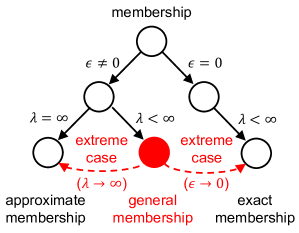
Figure 1. Our taxonomy.

Build on (carter1978exact, ), we develop a unified space lower bound $nf(\epsilon,\lambda)$ for general membership problems, which encompasses the prior theoretical results as extreme cases. Given a false positive rate $\epsilon$ and a negative-positive ratio $\lambda$, we have the following expression (where $H(\cdot)$ denotes Shannon’s entropy, ignore $o(1)$ terms):

$$\begin{cases}f\left(\epsilon,\lambda\right)=\underbrace{f\left(\epsilon^{\prime},\lambda\right)}_{\textbf{First stage}}+\underbrace{f\left(\epsilon/{\epsilon^{\prime}},\epsilon^{\prime}\lambda\right)}_{\textbf{Second stage}},\forall\epsilon^{\prime}\in[\epsilon,1]\text{ (Chain rule)};\\ f\left(0,\lambda\right)=\left(\lambda+1\right)H\left(\frac{1}{\lambda+1}\right)\text{ (Exact membership bound \text{\cite[citep]{(\@@bibref{AuthorsPhrase1Year}{carter1978exact}{\@@citephrase{, }}{})}})}.\end{cases}$$

Certainly, we can derive the arithmetic representation of $f$ by setting $\epsilon$ in chain rule to zero. However, we choose to retain the recursive formula because it offers valuable insights: According to the chain rule, any membership problem can be losslessly factorized into two (or multiple) stages. The first stage involves a coarse membership algorithm that may yield some false positive items, while the second stage employs an accurate membership algorithm to efficiently handle the remaining small percentage of false positive items, especially when the negative-positive ratio is very large. The chain rule reveals a non-trivial observation that the factorization process incurs zero information loss. This observation serves as inspiration for algorithm design and provides a solid theoretical foundation for future research in the field of membership problems.

Meanwhile, we acknowledge that the chain rule has certain limitations. First, it does not fully support dynamic memberships since it necessitates the identification of all false positive items before constructing the second stage. Moreover, we discover that the lossless property no longer holds for dynamic memberships (Section 4.3.1). Second, our chain rule theory is based on the assumption that all positive items are randomly selected from the universe, which may not perfectly accommodate real-world scenarios where item keys follow specific data distributions (Section 5.5).

$\bullet$ Paper Organization and Key Contributions.

(A, §2) We propose a space lower bound for general membership problems and derive an elegant factorization theorem called chain rule. This theorem allows us to divide any membership problem into sub-problems without losing information.

(B, §4) Building upon the chain rule, we introduce the versatile ChainedFilter framework, which enables the combination of multi-stage membership algorithms, such as Bloomier Filters, to construct more efficient algorithms. The framework is compatible with assorted elementary filters, supports different combining operators (e.g. AND and NAND), and can handle certain dynamic scenarios.

(C, §5) We evaluate the performance of ChainedFilter in data compressing, classifying and filtering applications. Experimental results show that although our utilization of chain rule in this paper is simple and rudimentary, the ChainedFilter can significantly outperform existing works: (1) it requires only 26% additional space over the theoretical lower bound for implicit static dictionary, (2) it requires only 0.22 additional bit per item over the theoretical lower bound for lossless data compression, (3) it reduces up to 31% external memory access than raw Cuckoo Hashing (fan2014cuckoo, ), (4) it reduces up to 36% P99 tail point query latency than Bloom Filter under the same space cost in RocksDB database (dong2021rocksdb, ), and (5) it reduces up to 99.1% filter space than original Learned Bloom Filter (kraska2018case, ; mitzenmacher2018model, ; liu2020stable, ; dai2020adaptive, ). We release our open source code on GitHub (opensourcecode, ).

$$\begin{split}\underbrace{\textbf{Chain rule}}_{\textbf{(A, \S\ref{algo::membership query}) Theory}}\xrightarrow[]{\textbf{design}}\underbrace{\textbf{ChainedFilter{}}}_{\textbf{(B, {\S\ref{algorithm}}) Algorithm}}\xrightarrow[]{\textbf{deploy}}\underbrace{\textbf{Applications}}_{\textbf{(C, \S\ref{perf}) Implementation}}\end{split}$$

2. Chain Rule Theory

Symbol	Description
$\mathcal{U}$	Universe (positive and negative items)
$\mathcal{S}$	The set of positive items
$\mathscr{S}$	The set of all possible sets of positive items ($\mathcal{S}$)
$n$	The number of positive items ($|\mathcal{S}|$)
$\epsilon$	False positive rate
$\lambda$	Negative-positive ratio ($|\mathcal{U}\backslash\mathcal{S}|/|\mathcal{S}|$)
$x$	An item
$C$	Any constant greater than 1
$M$	The number of buckets in one hash table
$r$	$|\mathcal{U}|/(2M)$
$N$	The number of SSTables in one level of LSM-Tree
$\sigma$	A mapping from $\mathscr{S}$ to $\mathscr{F}$
$\mathcal{X}_{\mathcal{F}}$	$\bigcup_{\mathcal{S}\in\sigma^{-1}(\mathcal{F})}\mathcal{S}$
$\mathcal{F}(\cdot)$	A specific filter
$\mathscr{F}$	The set of all possible filters ($\mathcal{F}$)
$nf(\cdot,\cdot)$	Space lower bound for membership problems
$nf^{\mathcal{F}}(\cdot,\cdot)$	Space cost of the membership filter $\mathcal{F}(\cdot)$
$H(\cdot)$	Shannon’s entropy
$h_{\alpha}(\cdot)$	$\alpha$-bit hash value of an item
$f_{\alpha}(\cdot)$	$\alpha$-bit fingerprint of an item
$T[\cdot]$	Hash table
BF/CF/EF	Bloomier Filter, ChainedFilter, elementary filter

Table 1. Commonly used symbols.

2.1. Definition and Notations

Given a universe $\mathcal{U}$ and arbitrary subset $\mathcal{S}\subset\mathcal{U}$, where $|\mathcal{U}|$ and $|\mathcal{S}|$ are known, the membership problem is to determine whether a queried item $x\in\mathcal{U}$ is in $\mathcal{S}$.

In this paper, we call a membership algorithm as a filter. This definition is broader than what people commonly use. A filter is an indicator function $\mathcal{F}(\cdot):\mathcal{U}\mapsto\{0,1\}$ with one-sided error, which means $\forall x\in\mathcal{S}$ (positive item), $\mathcal{F}(x)=1$ has zero false negative; for $x\in\mathcal{U}\backslash\mathcal{S}$ (negative item), we allow a small false positive rate $\epsilon\in[0,1]$ s.t. $\mathcal{F}(x)=1$. Moreover, we define $\lambda:=|\mathcal{U}\backslash\mathcal{S}|/|\mathcal{S}|$ as the negative-positive ratio, and we denote the membership problem as $(\epsilon,\lambda)$. This definition encompasses both approximate ($\epsilon\neq 0$ and $\lambda\to+\infty$) and exact ($\epsilon=0$ and $\lambda<+\infty$) membership problems as extreme cases. Unless specified otherwise, we assume that a filter is designed to handle static membership problems. If a membership filter also supports dynamic insertions of new items, we explicitly refer to it as a ”dynamic filter.” For quick reference, We list all commonly used symbols in Table 1. We will define some of these symbols in later sections.

2.2. Space Lower Bound

In this part, we present a unified and complete space lower bound for general membership problems.

Theorem 2.1.

(Space Lower Bound) Ignore $o(n)$ terms. Let $nf{(\epsilon,\lambda)}$ $:=n\inf\limits_{\mathcal{F}}\mathcal{F}({\epsilon,\lambda})$ be the space lower bound for general membership problem $(\epsilon,\lambda)$, we have

$$f(\epsilon,\lambda)=(\lambda+1)H\left(\frac{1}{\lambda+1}\right)-(\epsilon\lambda+1)H\left(\frac{1}{\epsilon\lambda+1}\right),$$

where $H(p):=-p\log p-(1-p)\log(1-p)\text{ is Shannon's entropy}.$

Proof.

The key idea of this proof follows the technique of (carter1978exact, ), except we take both $\epsilon$ and $\lambda$ into account. Given a membership problem ($\epsilon,\lambda$), we analysis all possible mappings from input sets to all possible filters, and use information theory to derive a lower bound of the space cost.

Given the universe $\mathcal{U}$ and the negative-positive ratio $\lambda$, we start by defining the set $\mathscr{S}:=\{\mathcal{S}\subset\mathcal{U}:|\mathcal{S}|=n\}$ as the set of all possible sets of positive items, and $\mathscr{F}$ as the set of all filter instances. Given any $\mathcal{S}\in\mathscr{S}$, we draw a filter instance $\mathcal{F}\in\mathscr{F}$ which has zero false negative. We denote this drawing method as a mapping $f:\mathscr{S}\mapsto\mathscr{F}$. Note that more than one set in $\mathscr{S}$ may map to a same filter $\mathcal{F}$, so the inverse mapping $\sigma^{-1}(\mathcal{F})\subset\mathscr{S}$ may have more than one element. Actually, we have

$$\sum\limits_{\mathcal{F}\in\mathscr{F}}|\sigma^{-1}(\mathcal{F})|=|\mathscr{S}|=\binom{|\mathcal{U}|}{|\mathcal{U}\backslash\mathcal{S}|}\text{ and }|\mathscr{F}|\leqslant 2^{nf(\epsilon,\lambda)}.$$

Since the filter $\mathcal{F}$ has zero false negative, so for every $x\in\mathcal{X}_{\mathcal{F}}:=\bigcup\limits_{\mathcal{S}\in\sigma^{-1}(\mathcal{F})}\mathcal{S}$, we have $\mathcal{F}(x)=1$ (Figure 2).

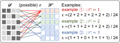
Figure 2. Some examples when $\mathcal{U}=\{1,2,3,4\}$ and $|\mathcal{S}|=2$ (i.e.$\mathscr{S}=\{\{1,2\},\{1,3\},\{1,4\},\{2,3\},\{2,4\},\{3,4\}\})$. All connections are possible (but maybe not unique) mappings. The mapping should ensure that the filter has a zero false negative rate. For instance, in example 2, $\sigma$ maps the input positive set $\mathcal{S}=\{1,2\}$ (the first row on the left) to the first green filter $\mathcal{F}$ s.t. $\mathcal{X}_{\mathcal{F}}=\{1,2,3\}$. In other words, $\mathcal{F}(1)=1,\mathcal{F}(2)=1,\mathcal{F}(3)=1$ (false positive), and $\mathcal{F}(4)=0$.

The next two formulae are the critical observations in our proof: On the one hand, since the elements in $\sigma^{-1}(\mathcal{F})$ are different from each other, we have

$$\binom{|\mathcal{X}_{\mathcal{F}}|}{|\mathcal{S}|}\geqslant|\sigma^{-1}(\mathcal{F})|;$$

On the other hand, for a specific $\mathcal{S}\in\sigma^{-1}(\mathcal{F})$ and for all $x\in\mathcal{U}$, $\mathcal{F}(x)=1$ incurs false positive iff $x\in X_{\mathcal{F}}\backslash\mathcal{S}$. Therefore, the overall false positive rate is

$$\epsilon=\frac{\sum\limits_{\mathcal{F}\in\mathscr{F}}|\sigma^{-1}(\mathcal{F})|\frac{|\mathcal{X}_{\mathcal{F}}\backslash\mathcal{S}|}{|\mathcal{U}\backslash\mathcal{S}|}}{\sum\limits_{\mathcal{F}\in\mathscr{F}}|\sigma^{-1}(\mathcal{F})|}.$$

Now let $\theta>0$, our main idea of the following proof is to divide $\mathscr{F}$ into two parts $\mathscr{F}_{1}:=\{\mathcal{F}\in\mathscr{F}:|X_{\mathcal{F}}\backslash\mathcal{S}|\geqslant\theta n\}$ and $\mathscr{F}_{2}:=\mathscr{F}\backslash\mathscr{F}_{1}$, then bound their false positive rate respectively.

Consider the monotonically increasing function $g(p):=\exp\{n((p+1)\ln(p+1)-p\ln p)\}(p>0)$. To start with, we prove $\forall\varepsilon\in(0,1),\exists N_{0}>0,s.t.\forall\mathcal{F}\in\mathscr{F}_{1},$ when $n>N_{0},\varepsilon g^{-1}(|\sigma^{-1}(\mathcal{F})|)n$ is uniformly less than $|X_{\mathcal{F}}\backslash\mathcal{S}|.$ Initially, given $\varepsilon<\varepsilon^{\prime}<1$, we can select $N_{1}=(\varepsilon^{\prime}-\varepsilon)^{-1}$ s.t. when $n>N_{1},$ we have $\varepsilon g^{-1}(|\sigma^{-1}(\mathcal{F})|)n<\varepsilon^{\prime}g^{-1}(|\sigma^{-1}(\mathcal{F})|)n$ $-1<\lfloor\varepsilon^{\prime}g^{-1}(|\sigma^{-1}(\mathcal{F})|)n\rfloor.$ Next, according to Stirling’s formula

$$\lim\limits_{n\to+\infty}\frac{n!}{\sqrt{2\pi n}}\left(\frac{e}{n}\right)^{n}=1,$$

we can select $N_{0}>N_{1}$ which only relies on $\varepsilon$ and $\theta$, s.t. $\forall n>N_{0}$, $\tbinom{\lfloor\varepsilon^{\prime}g^{-1}(|\sigma^{-1}(\mathcal{F})|)n\rfloor+|\mathcal{S}|}{|\mathcal{S}|}<2g(\varepsilon^{\prime}g^{-1}(|\sigma^{-1}(\mathcal{F})|))<g(g^{-1}(|\sigma^{-1}(\mathcal{F})|))$ $=|\sigma^{-1}(\mathcal{F})|\leqslant\tbinom{|\mathcal{X}_{\mathcal{F}}|}{|\mathcal{S}|}\Rightarrow\varepsilon g^{-1}(|\sigma^{-1}(\mathcal{F})|)n<\lfloor\varepsilon^{\prime}g^{-1}(|\sigma^{-1}(\mathcal{F})|)n\rfloor<|X_{\mathcal{F}}\backslash\mathcal{S}|$ holds for all $\mathcal{F}\in\mathscr{F}_{1}$.

Similarly, when $n\to+\infty,$ we have $|\sigma^{-1}(\mathcal{F})|<g(2\theta)$ for all $\mathcal{F}\in\mathscr{F}_{2}$. Therefore

$$\sum\limits_{\mathcal{F}\in\mathscr{F}_{1}}|\sigma^{-1}(\mathcal{F})|\geqslant|\mathscr{S}|-g(2\theta)|\mathscr{F}|.$$

To take a step further, consider $h(p):=pg^{-1}(p):=xp.$ Because

$$\frac{\mathrm{d}h(p)}{\mathrm{d}p}=y+p/\left(\frac{\mathrm{d}g^{-1}(y)}{\mathrm{d}y}\right)=y+\frac{1}{n\ln(y+1)-n\ln y}$$

increases as $y$ increases (so as $p=g^{-1}(y)$ increases), we find $h$ convex. According to Jensen’s inequality, we have

$$\begin{split}\epsilon&\geqslant\frac{\sum\limits_{\mathcal{F}\in\mathscr{F}_{1}}|\sigma^{-1}(\mathcal{F})|\frac{|\mathcal{X}_{\mathcal{F}}\backslash\mathcal{S}|}{|\mathcal{U}\backslash\mathcal{S}|}}{\sum\limits_{\mathcal{F}\in\mathscr{F}}|\sigma^{-1}(\mathcal{F})|}\geqslant\frac{\sum\limits_{\mathcal{F}\in\mathscr{F}_{1}}|\sigma^{-1}(\mathcal{F})|\varepsilon g^{-1}(|\sigma^{-1}(\mathcal{F})|)n}{|\mathscr{S}|\lambda n}\\ &\geqslant\frac{\varepsilon}{|\mathscr{S}|\lambda}\left(\sum\limits_{\mathcal{F}\in\mathscr{F}_{1}}|\sigma^{-1}(\mathcal{F})|\right)g^{-1}\left(\frac{\sum\limits_{\mathcal{F}\in\mathscr{F}_{1}}|\sigma^{-1}(\mathcal{F})|}{|\mathscr{F}_{1}|}\right)\end{split}$$

$$\begin{split}&\geqslant\frac{\varepsilon}{\lambda}\left(1-\frac{g(2\theta)|\mathscr{F}|}{|\mathscr{S}|}\right)g^{-1}\left(\frac{|\mathscr{S}|}{|\mathscr{F}|}-g(2\theta)\right).\end{split}$$

Let $\varepsilon\to 1,\theta\to 0$ and ignore $o(n)$, we have

$$\epsilon\lambda\geqslant g^{-1}\left(\frac{|\mathscr{S}|}{|\mathscr{F}|}\right)\Rightarrow g(\epsilon\lambda)\geqslant\frac{|\mathscr{S}|}{|\mathscr{F}|}\geqslant\frac{g(\lambda)}{2^{nf({\epsilon,\lambda})}}.$$

Therefore

$$f({\epsilon,\lambda})\geqslant\frac{1}{n}\log\frac{g(\lambda)}{g(\epsilon\lambda)}=\log\left(\frac{(\lambda+1)^{\lambda+1}}{\lambda^{\lambda}}\right)-\log\left(\frac{(\epsilon\lambda+1)^{\epsilon\lambda+1}}{(\epsilon\lambda)^{\epsilon\lambda}}\right).$$

It’s easy to verify that $f({\epsilon,\lambda})\leqslant\frac{1+o(1)}{n}(\log g(\lambda)-\log g(\epsilon\lambda))$ (consider the example $\binom{|\mathcal{X}_{\mathcal{F}}|}{|\mathcal{S}|}=(|\mathscr{S}|/|\mathscr{F}|)(1+o(1))$). So

$$f({\epsilon,\lambda})=(\lambda+1)H\left(\frac{1}{\lambda+1}\right)-(\epsilon\lambda+1)H\left(\frac{1}{\epsilon\lambda+1}\right)$$

is the space lower bound. ∎

Remark 0.

Theorem 2.1 connects the approximate and the exact membership query problems. When $\epsilon\neq 0$ and $\lambda\to+\infty$, $f({\epsilon,+\infty})=\log 1/\epsilon$ degenerates to the space lower bound of approximate memberships. When $\epsilon=0$ and $\lambda<+\infty$, $f({0,\lambda})=(\lambda+1)H\left(1/(\lambda+1)\right)$ degenerates to the space lower bound of exact memberships (carter1978exact, ).

2.3. Chain Rule

In this part, we delve deeper and derive our chain rule theory, which is arithmetically equivalent to the space lower bound but provides insights into the essence of membership problems. As a preliminary, please note that in our context, the term “membership problem” is different from the term “membership filter”. When referring to an abstract “problem”, we focus on the theoretical space lower bound. While when discussing a specific “filter”, we focus on a practical algorithm that may not be space-optimal.

To begin, let’s consider encoding $n$ positive items and $\lambda n$ negative items with a false positive rate of $\epsilon_{1}\epsilon_{2}$. Intuitively, we can factorize the problem into two stages: first, encoding all positive items and the $\lambda n$ negative items with a false positive rate of $\epsilon_{1}$, and then encoding the positive items and the remaining $\lambda\epsilon_{1}n$ false positive items with a false positive rate of $\epsilon_{2}$. It is evident that if we solve the two sub-problems, we can address the primary problem. Hence, the two sub-problems should not be easier than the primary problem. However, since the positive items are encoded twice in separate stages, it may seem that the two-stage factorization incurs additional space overhead, and we might need to make careful trade-offs to avoid accumulating inherent space costs caused by the factorization.

Surprisingly, Theorem 2.1 reveals that all our concerns and worries are unnecessary. Because

$$\begin{split}f(\epsilon_{1}\epsilon_{2},\lambda)&=(\lambda+1)H\left(\frac{1}{\lambda+1}\right)-(\epsilon_{1}\epsilon_{2}\lambda+1)H\left(\frac{1}{\epsilon_{1}\epsilon_{2}\lambda+1}\right)\\ &=\left((\lambda+1)H\left(\frac{1}{\lambda+1}\right)-(\epsilon_{1}\lambda+1)H\left(\frac{1}{\epsilon_{1}\lambda+1}\right)\right)\\ &+\left((\epsilon_{1}\lambda+1)H\left(\frac{1}{\epsilon_{1}\lambda+1}\right)-(\epsilon_{1}\epsilon_{2}\lambda+1)H\left(\frac{1}{\epsilon_{1}\epsilon_{2}\lambda+1}\right)\right)\\ &=f(\epsilon_{1},\lambda)+f(\epsilon_{2},\epsilon_{1}\lambda),\end{split}$$

we find the factorization is completely lossless (ignoring $o(1)$ terms), which means we can arbitrarily decompose any membership problem into an arbitrary number of sub-problems without incurring any additional space cost. In other words, if all the elementary filters used in the combination are space-optimal, the resulting combined membership filter will also be space-optimal. Instead, when we combine imperfect membership filters to solve a membership problem, the only source of space overhead stems from that the filters cannot optimally solve the sub-problems. The factorization process itself does not introduce any additional space overhead. In later chapters, we will use Bloomier Filters as a straightforward example to show how to appropriately factorize a membership problem into sub-problems and enhance overall performance. But before that, let us rewrite the expressions as $\epsilon=\epsilon_{1}\epsilon_{2}$ and $\epsilon^{\prime}=\epsilon_{1}$, and present the conclusion in a recursive form:

Theorem 2.2.

(Chain Rule Theory)

$$\begin{cases}f\left(\epsilon,\lambda\right)={f\left(\epsilon^{\prime},\lambda\right)}+{f\left(\epsilon/{\epsilon^{\prime}},\epsilon^{\prime}\lambda\right)},\forall\epsilon^{\prime}\in[\epsilon,1];\\ f\left(0,\lambda\right)=\left(\lambda+1\right)H\left(\frac{1}{\lambda+1}\right).\end{cases}$$

It’s easy to verify that the above equation set is equivalent to the space lower bound in Theorem 2.1 (you can check it by setting $\epsilon=0$), but this form is more elegant and may provide more insights.

3. Bloomier Filter

In this section, we present two variants derived from the Bloomier Filter (chazelle2004bloomier, ; charles2008bloomier, ), which belong to approximate and exact membership algorithms, respectively. In Section 4, we combine these elementary filters by chain rule to construct ChainedFilter. The reason we introduce Bloomier Filters as elementary filters is that they are easy to describe and implement, but readers can also use other elementary filters to achieve special properties, like smaller filter space, smaller construction space or supporting dynamic exclusions. We discuss more related works in Section 6.

Overview. Bloomier Filter is a compact perfect hashing algorithm that supports both approximate and exact membership query by encoding item $e$’s fingerprint $f_{\alpha}(e)\in\{0,1\}^{\alpha}$ into the hash table. Specifically, to build an approximate membership algorithm, the Bloomier Filter encodes an $\alpha$-bit fingerprint $f_{\alpha}(e)=h_{\alpha}(e)$ for every positive item; to build an exact membership algorithm, the Bloomier Filter maps every item to a one-bit hash value $h_{1}(e)\in\{0,1\}$ and encodes $f_{1}(e)=h_{1}(e)$ (resp. $f_{1}(e)=\sim h_{1}(e)$) for every positive (resp. negative) item. The query result of an item $e$ depends on whether its hash value matches the fingerprint in the hash table. For interested readers, we present the detailed descriptions of Bloomier Filter in the next three paragraphs. Skipping them and directly reading the Remark does not affect the comprehension of this paper.

Algorithm. Suppose we already have the entire universe of all $|\mathcal{U}|$ possible items whose value are either zero or one. To construct the hash table, we first initialize the hash table by all zero, mark all items as “not matched” and let the variable $order=|\mathcal{U}|$. the Bloomier Filter maps every not-matched item $e$ to $j$ different slots $s^{e}_{[1..j]}$. Then, it repeats the following operations (called the peeling process) until all items are “matched”: (1) It selects a slot $s$ that is mapped by only one item $e_{0}$; (2) It marks the insertion place (ip) of $e_{0}$ as $s(e_{0})=s$, and the insertion order (io) of $e_{0}$ as $order$; (3) It marks $e_{0}$ as “matched”, peels $e_{0}$ and decreases $order$ by one. Finally, it inserts items in $order$: for items $e$ from $order=1$ to $|\mathcal{U}|$, it encodes $(\oplus_{i=1}^{j}s^{e}_{i})\oplus f_{\alpha}(e)$(where $\oplus$ means XOR) into the slot $s(e)$. To query an item $e$, the Bloomier Filter reports $\oplus_{i=1}^{j}s^{e}_{i}$ as the result.

Example. Suppose we have $|\mathcal{U}|=3$ items $e_{1},e_{2}$ and $e_{3}$. To construct the hash table, the Bloomier Filter first maps $e_{1}$ to $i=3$ slots $s_{1},s_{2},s_{3}$; maps $e_{2}$ to $s_{1},s_{3},s_{4}$; and maps $e_{3}$ to $s_{2},s_{4},s_{5}$. Then the filter (1) selects slot $s_{5}$ which is only mapped by $e_{3}$, marks $e_{3}$ with (ip = 5, io = 3) and peels $e_{3}$; (2) selects $s_{2}$ which is only mapped by $e_{1}$, marks $e_{1}$ with (ip = 2, io = 2) and peels $e_{1}$; (3) selects $s_{1}$ which is only mapped by $e_{2}$, marks $e_{2}$ with (ip = 1, io = 1) and peels $e_{2}$. Finally, the filter (1) inserts $s_{1}$ with $s_{1}\oplus s_{3}\oplus s_{4}\oplus f_{\alpha}(e_{2})=f_{\alpha}(e_{2})$ (io = 1); (2) inserts $s_{2}$ with $s_{1}\oplus s_{2}\oplus s_{3}\oplus f_{\alpha}(e_{1})=f_{\alpha}(e_{2})\oplus f_{\alpha}(e_{1})$ (io = 2); (3) inserts $s_{5}$ with $s_{2}\oplus s_{4}\oplus s_{5}\oplus f_{\alpha}(e_{3})=f_{\alpha}(e_{2})\oplus f_{\alpha}(e_{1})\oplus f_{\alpha}(e_{3})$ (io = 3). To query the items, the Bloomier Filter reports $Query(e_{1})=s_{1}\oplus s_{2}\oplus s_{3}=(f_{\alpha}(e_{2}))\oplus(f_{\alpha}(e_{2})\oplus f_{\alpha}(e_{1}))\oplus 0=f_{\alpha}(e_{1}),Query(e_{2})=s_{1}\oplus s_{3}\oplus s_{4}=(f_{\alpha}(e_{2}))\oplus 0\oplus 0=f_{\alpha}(e_{2}),\text{ and }Query(e_{3})=s_{2}\oplus s_{4}\oplus s_{5}=(f_{\alpha}(e_{2})\oplus f_{\alpha}(e_{1}))\oplus 0\oplus(f_{\alpha}(e_{2})\oplus f_{\alpha}(e_{1})\oplus f_{\alpha}(e_{3}))=f_{\alpha}(e_{3})$.

Theory. The theory underlying the Bloomier Filter is highly non-trivial (goodrich2011invertible, ). The peeling process mentioned above is actually equivalent to finding the 2-core of random hypergraph. If the number of potential slots is greater than $cN$, where $c$ is any constant larger than

$$c_{j}^{-1}:=\left(\sup\left\{\alpha\in(0,1):\forall x\in(0,1),1-e^{-j\alpha x^{j-1}}<x\right\}\right)^{-1},$$

the peeling process will succeed with high probability $1-o(1)$. We denote $c_{j}^{-1}$ as the threshold which achieves its minimum value $1.23$ when $j=3$. Recently, this result is optimized by (walzer2021peeling, ) (2021) which proposes a new distribution of hyperedges. The author selects $j$ slots uniformly at random from a range of $|\mathcal{U}|/(z+1)$ slots, improving the threshold close to $c_{j}^{\prime-1}$, where $c_{j}^{\prime-1}$ can be arbitrarily close to 1 (e.g. $c_{3}^{\prime-1}\approx 1.12,c_{4}^{\prime-1}\approx 1.05$ when $z=120$). In Section 5, we set $j=3,z=120,$ and $C=1.13$ to conduct experiments.

Remark 0.

To conclude, the Bloomier Filter can derive space-efficient approximate ($Cn\log 1/\epsilon$ bits) and exact ($C|\mathcal{U}|$ bits) membership filters, where $C$ can be an arbitrary constant close to 1. Interestingly, the two formulae have completely different forms, which seemingly leave room for improvement. This simple observation inspires us to bridge the gap between the two variants to obtain a better theoretical result.

4. ChainedFilter

4.1. Key Insight

We use the exact membership ChainedFilter as an example to illustrate our key insight. Now let’s recap the theoretical results of the approximate and the exact variants of Bloomier Filters (BF) shown in the Remark of Section 3:

$$\begin{cases}f^{BF}({\epsilon,\lambda})\leqslant f^{BF}(\epsilon,+\infty)=C\log 1/\epsilon&\text{(Approximate)};\\ f^{BF}({0,\lambda})=C(\lambda+1)&\text{(Exact)}.\end{cases}$$

According to Theorem 2.2, we can losslessly factorize a membership problem ($0,\lambda$) into two sub-problems ($\epsilon^{\prime},\lambda$) and ($0,\epsilon^{\prime}\lambda$), and use Bloomier Filters as elementary filters to form ChainedFilter s.t.

$$f^{CF}(0,\lambda)=f^{BF}(\epsilon^{\prime},\lambda)+f^{BF}(0,\epsilon^{\prime}\lambda)\leqslant C\log 1/\epsilon^{\prime}+C(\epsilon^{\prime}\lambda+1).$$

Because $\epsilon^{\prime}$ can be any value between 0 and 1, we can minimize $f^{CF}(0,\lambda)$ to $C\log(2e\lambda\ln 2)$ by setting $\epsilon^{\prime}=1/(\lambda\ln 2).$ Such an intuitive technique amazingly makes $f^{CF}(0,\lambda)$ less than $1.11f({0,\lambda})$.

Input: Universe $\mathcal{U}$ and subset $\mathcal{S}$, $|\mathcal{U}|/|\mathcal{S}|=\lambda>1/\ln 2$.

Output: A filter $\mathcal{F}:\mathcal{U}\mapsto\{0,1\}$ s.t. $\mathcal{F}(e)=1$ iff $e\in S$.

1 Function Construct ($\mathcal{U},\mathcal{S}$):

2 Set $\log 1/\epsilon=\lfloor\log\lambda\rfloor$ and the false positive set $\mathcal{S}^{\prime}=\emptyset.$

3 Construct an approximate membership filter $\mathcal{F}_{1}$ s.t.

$$\begin{cases}\mathcal{F}_{1}(e)=1,&\forall e\in\mathcal{S};\\ \mathbb{P}[\mathcal{F}_{1}(e)=0]=\epsilon,&\forall e\in\mathcal{U}\backslash\mathcal{S}.\end{cases}$$

For all $e\in\mathcal{U}\backslash\mathcal{S}$ satisfying $\mathcal{F}_{1}(e)=1:$ Insert $e$ into $\mathcal{S}^{\prime}.$

Construct an exact filter $\mathcal{F}_{2}$ s.t.

$$\begin{cases}\mathcal{F}_{2}(e)=1,&\forall e\in\mathcal{S};\\ \mathcal{F}_{2}(e)=0,&\forall e\in\mathcal{S}^{\prime}.\\ \end{cases}$$

return $\mathcal{F}(\cdot):=\mathcal{F}_{1}(\cdot)$ & $\mathcal{F}_{2}(\cdot)$.

Algorithm 1 ChainedFilter for Exact Membership Query

This exact membership example demonstrates the potential of the chain rule. We summarize it in Algorithm 1 and Figure 3, and show its experimental performance in Section 5.1. To construct ChainedFilter, in step ①, we first encode all the positive items into a $Cn\log(\lambda\ln 2)$-bit approximate Bloomier Filter with false positive rate $\epsilon=1/(\lambda\ln 2)$ (Line 3). In step ②, we query all negative and collect the false positive ones into a set $\mathcal{S}^{\prime}$ (Line 4). In step ③, we encode all the positive as well as all the false positive items (i.e. items in $\mathcal{S}^{\prime}$) into a $Cn\log 2e$-bit Exact Bloomier Filter (Line 5). In this way, the overall space cost $nf^{CF}({0,\lambda})$ is minimized. To query an item, we query both of the two filters and report their AND value as the result (Line 6).

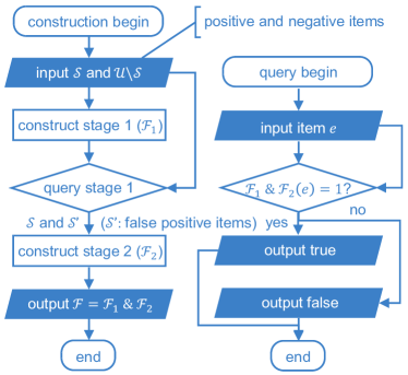
Figure 3. ChainedFilter shown in Section 4.1.

4.2. Generalization and Analysis

In this part, we (1) extend the exact ($\epsilon=0$) ChainedFilter to a general ($\epsilon\neq 0$) ChainedFilter and show that the two-stage structure is space-optimal, (2) extend Bloomier Filters to an arbitrary number of elementary filters and reveal ChainedFilter’s limitation. Since this part is only technically complex, skipping it does not affect the comprehension of this paper.

4.2.1. ChainedFilter for general membership query

Since the trivial theoretical bound

$$f^{CF}({\epsilon,\lambda})\leqslant\min\left\{f^{CF}({0,(1-\epsilon)\lambda}),tf^{CF}({\epsilon,\lambda/t})\right\}(\forall t>1)$$

is too loose, we introduce additional inequalities to reduce error. The key observation is that an $C(\beta+1)n(\beta>0)$-bit Bloomier Filter can also filter out some negative items that are not encoded in the perfect hash table. Recall that in Section 3, we say a Bloomier Filter encodes a one-bit fingerprint $f_{1}(e)=h_{1}(e)\in\{0,1\}$ (resp. $\sim h_{1}(e)$) for a positive (resp. negative) item. Now let’s consider two strategies for generating $h_{1}(e)$. (a) The first strategy is $\mathbb{P}[h_{\alpha}(\cdot)=1]=1/2$, which means we flip a fair coin and record the face up side (resp. face down side) as the fingerprint of a positive (resp. negative) item. In this way, only 1/2 not-encoded negative items are false positive items. (b) The second strategy is $\mathbb{P}[h_{\alpha}(\cdot)=1]=1$, which means we directly record 1 (resp. 0) as the fingerprint of a positive (resp. negative) item. In this way, only $1/(\beta+1)$ not-encoded negative items are false positive items. These strategies give rise to two additional inequalities (BF represents ChainedFilter. When the equation “=” holds, the algorithm degenerates to one single Bloomier Filter)

$$\begin{cases}f^{CF}({\epsilon,\lambda})/C\leqslant\lambda+1-2\epsilon\lambda\quad\quad\quad(\epsilon\leqslant 2\lambda/(\lambda+1))&(a);\\ f^{CF}({\epsilon,\lambda})/C\leqslant(\lambda+1)/(\epsilon\lambda+1)\quad(\epsilon\leqslant 1/2)&(b).\end{cases}$$

Similar to the exact ChainedFilter (Algorithm 1), the generalized algorithm also consists of one approximate Bloomier Filter and one exact Bloomier Filter. The only difference is, the approximate Bloomier Filter requires $Cn\alpha=Cn(f^{CF}({\epsilon,\lambda})-\beta-1)$ bits and has a false positive rate of $1/2^{\alpha}$, while the Exact Bloomier Filter requires $Cn(\beta+1)$ bits and has a false positive rate of $\min\{1/2,1/(\beta+1)\}$. Using the two inequalities and the chain rule, we can determine the optimal parameter settings of $\alpha,\beta$ and thus $f^{CF}({\epsilon,\lambda})$. Because the calculation process is a bit dry, we present the results directly in Corollary 4.1 and Figure 4.

Corollary 4.1.

if we only combine two Bloomier Filters, the optimal space cost and the corresponding parameters are

$$f^{CF}({\epsilon,\lambda}):=\min\left\{f^{(a)}({\epsilon,\lambda}),f^{(b)}({\epsilon,\lambda})\right\},$$

where $f^{(a)}({\epsilon,\lambda}),f^{(b)}({\epsilon,\lambda})$ are defined as follows:

$$\begin{split}\text{(a)}&\text{ If }\lambda>\frac{1}{\ln 2}\text{ and }\lambda<\frac{1}{2\epsilon\ln 2}\text{, then }\mathbb{P}[h_{\alpha}(\cdot)=1]=1/2,\end{split}$$

$$\begin{split}&\beta_{(a)}=\frac{1}{\ln 2}-2\lambda\epsilon\text{ and }f^{(a)}({\epsilon,\lambda})/C=\log(2e\lambda\ln 2)-2\lambda\epsilon.\\ &\text{ Otherwise $f^{(a)}({\epsilon,\lambda})$ degenerates to the space of approximate }\\ &(\beta=0)\text{ or exact }(\alpha=0)\text{ Bloomier Filters.}\\ \text{(b)}&\text{ If }\lambda>\frac{1}{\ln 2-\epsilon}>0\text{, then }\mathbb{P}[h_{\alpha}(\cdot)=1]=1,\\ &\beta_{(b)}=\frac{1}{\ln 2}-\frac{\epsilon\lambda}{\epsilon\lambda+1},\text{ and }f^{(b)}({\epsilon,\lambda})/C=\log\frac{2e\lambda\ln 2}{\epsilon\lambda+1}-\frac{\epsilon\lambda}{\epsilon\lambda+1}.\\ &\text{ Otherwise $f^{(b)}({\epsilon,\lambda})$ degenerates to the space of approximate }\\ &(\beta=0)\text{ or exact }(\alpha=0)\text{ Bloomier Filters.}\\ \end{split}$$

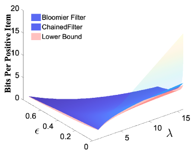
Figure 4. Space cost when $C\to 1$. The multicolored surface is the minimum space cost of a single Bloomier Filter. When $\epsilon=0$ and $\lambda=16$, it is 210% higher than the theoretical lower bound, while the space overhead of ChainedFilter (the blue surface) is only 8%.

4.2.2. Two filters can be optimal

It seems that only two stages is too trivial. But interestingly, we prove that combining two Bloomier Filters using operator “&” is space-optimal.

Theorem 4.1.

(Optimality) Suppose we have a combined filter $\mathcal{F}:=\&_{i=1}^{m}\mathcal{F}_{i}$, where $\mathcal{F}_{i}$ are Bloomier Filters. Then we can prove that (CF represents ChainedFilter)

$$f^{\mathcal{F}}({\epsilon,\lambda})\geqslant f^{CF}({\epsilon,\lambda}).$$

Proof.

We only consider inequality $(a)$, i.e. $f^{BF}({\epsilon,\lambda})/C=\lambda+1-2\epsilon\lambda(\epsilon\leqslant 2\lambda/(\lambda+1))$, where BF represents Bloomier Filter, because the case for inequality $(b)$ is similar.

Let $\epsilon:=\epsilon_{1}\epsilon_{2}...\epsilon_{m}$, according to the chain rule

$$\begin{split}f(\epsilon,\lambda)&=f(\epsilon_{1},\lambda)+f(\frac{\epsilon}{\epsilon_{1}},\epsilon_{1}\lambda)\\ &=f(\epsilon_{1},\lambda)+f(\epsilon_{2},\epsilon_{1}\lambda)+f(\frac{\epsilon}{\epsilon_{1}\epsilon_{2}},\epsilon_{1}\epsilon_{2}\lambda)\\ &=f(\epsilon_{1},\lambda)+f(\epsilon_{2},\epsilon_{1}\lambda)+f(\epsilon_{3},\epsilon_{1}\epsilon_{2}\lambda)+f(\frac{\epsilon}{\epsilon_{1}\epsilon_{2}\epsilon_{3}},\epsilon_{1}\epsilon_{2}\epsilon_{3}\lambda)\\ &=...\\ &=f(\epsilon_{1},\lambda)+f(\epsilon_{2},\epsilon_{1}\lambda)+...+f(\epsilon_{m},\epsilon_{1}\epsilon_{2}...\epsilon_{m-1}\lambda),\\ \end{split}$$

we have

$$\begin{split}\min\limits_{\mathcal{F}}&f^{\mathcal{F}}({\epsilon,\lambda})/C=\min\limits_{\epsilon_{1},\epsilon_{2},...,\epsilon_{m}\in[0,1/2]}^{\epsilon_{1}\epsilon_{2}...\epsilon_{m}=\epsilon}\sum\limits_{i=1}^{m}f^{BF}({\epsilon_{i},\epsilon_{1}\epsilon_{2}...\epsilon_{i-1}\lambda})/C\\ &=m+(1-2\epsilon)\lambda-\max\limits_{\epsilon_{1},\epsilon_{2},...,\epsilon_{m-1}\in[0,1/2]}\left(\sum\limits_{i=1}^{m-1}\prod\limits_{j=1}^{i}\epsilon_{j}\right)\lambda\\ &=m+(1-2\epsilon)\lambda-\left(1-\frac{1}{2^{m-1}}\right)\lambda=\left(m+\frac{\lambda}{2^{m-1}}\right)-2\epsilon\lambda.\end{split}$$

$$\text{When }\begin{cases}m=\lfloor\log\lambda\rfloor+1;\\ \epsilon_{1}=...=\epsilon_{m-1}=1/2;\\ \epsilon_{m}=2^{m-1}\epsilon,\end{cases}$$

The formula achieves the minimum value

$$f^{\mathcal{F}}({\epsilon,\lambda})=\lfloor\log\lambda\rfloor+1+\frac{\lambda}{2^{\lfloor\log\lambda\rfloor}}-2\epsilon\lambda=f^{CF}({\epsilon,\lambda}).$$

So ChainedFilter is space-optimal. ∎

Remark 0.

When $\epsilon=0$, the rounded space cost of ChainedFilter is

$$f^{CF}({0,\lambda})=C(\lfloor\log\lambda\rfloor+1+\frac{\lambda}{2^{\lfloor\log\lambda\rfloor}})<1.11Cf({0,\lambda}).$$

We will recap this result in Section 5.1 and 5.2.

4.2.3. Limitation of the operator “&”

When the elementary filters are not limited to Bloomier Filters, the optimal combined filter can be very complex. In fact, we may not even know how many elementary filters we should use. However, we find that if we continue to use the “&” operator to combine filters, we can derive the tight space lower bound of the combined filter.

Theorem 4.2.

(Limitation) Given arbitrary elementary filters (EF) $\mathcal{F}_{i}$ with a restriction of $f^{EF}({\epsilon,\lambda})$ and an arbitrary combined filter $\mathcal{F}:=\&_{i=1}^{m}\mathcal{F}_{i}$. We define $\mathchar 265\relax^{EF}({\epsilon,\lambda}):[0,1]\times\mathbb{R}^{+}\mapsto\mathbb{R}$ as any function satisfying

$$\begin{cases}f({\epsilon,\lambda})\leqslant\mathchar 265\relax^{EF}({\epsilon,\lambda})\leqslant f^{EF}({\epsilon,\lambda})&\forall\epsilon\in[0,1],\\ \mathchar 265\relax^{EF}({\epsilon_{1}\epsilon_{2},\lambda})\leqslant\mathchar 265\relax^{EF}({\epsilon_{1},\lambda})+\mathchar 265\relax^{EF}({\epsilon_{2},\epsilon_{1}\lambda})&\forall\epsilon_{1},\epsilon_{2}\in[0,1].\end{cases}$$

Then we have

$$\inf f^{\mathcal{F}}({\epsilon,\lambda})=\sup\mathchar 265\relax^{EF}({\epsilon,\lambda}).$$

Proof.

First, we assert that (1) $\inf f^{\mathcal{F}}({\epsilon,\lambda})$ exists. This is because $f^{\mathcal{F}}({\epsilon,\lambda})$ exists ($f^{\mathcal{F}}({\epsilon,\lambda})\leqslant f^{EF}({\epsilon,\lambda})$) and has an lower bound $f({\epsilon,\lambda})$. (2) $\sup\mathchar 265\relax^{EF}({\epsilon,\lambda})$ exists. This is because $\mathchar 265\relax^{EF}({\epsilon,\lambda})$ exists ($\mathchar 265\relax^{EF}({\epsilon,\lambda})\geqslant f({\epsilon,\lambda})$) and has an upper bound $f^{EF}({\epsilon,\lambda})$.

Second, we prove that $f^{\mathcal{F}}({\epsilon,\lambda})\geqslant\mathchar 265\relax^{EF}({\epsilon,\lambda})$ by mathematical induction. When $m=1$ (note that $m$ is the number of elementary filters), we observe $f^{\mathcal{F}}({\epsilon,\lambda})=f^{EF}({\epsilon,\lambda})\geqslant\mathchar 265\relax^{EF}({\epsilon,\lambda}).$ Assume that when $m=m_{0}-1$ we have $f^{\mathcal{F}}({\epsilon,\lambda})\geqslant\mathchar 265\relax^{EF}({\epsilon,\lambda})$. Then, when $m=m_{0},$ we can rewrite $\mathcal{F}$ as $(\&_{i=1}^{m_{0}-1}\mathcal{F}_{i})\&\mathcal{F}_{m_{0}}.$ W.l.o.g., we can assume that $\&_{i=1}^{m_{0}-1}\mathcal{F}_{i}$ encodes $\lambda n$ negative items with false positive rate $\epsilon^{\prime}$, and $\mathcal{F}_{m_{0}}$ encodes $\lambda^{\prime}n(\lambda^{\prime}\geqslant\epsilon^{\prime}\lambda)$ negative items with false positive rate $\epsilon^{\prime\prime}(\epsilon^{\prime}\epsilon^{\prime\prime}\leqslant\epsilon)$. Thus

$$\begin{split}f^{\mathcal{F}}({\epsilon,\lambda})&\geqslant\mathchar 265\relax^{EF}({\epsilon^{\prime},\lambda})+\mathchar 265\relax^{EF}({\epsilon^{\prime\prime},\lambda^{\prime}})\\ &\geqslant\mathchar 265\relax^{EF}({\epsilon^{\prime},\lambda})+\mathchar 265\relax^{EF}({\epsilon^{\prime\prime},\epsilon\lambda})\\ &\geqslant\mathchar 265\relax^{EF}({\epsilon^{\prime}\epsilon^{\prime\prime},\lambda})\geqslant\mathchar 265\relax^{EF}({\epsilon,\lambda}).\end{split}$$

Therefore, $\forall m\in\mathbb{N}^{+}$ we have

$$f^{\mathcal{F}}({\epsilon,\lambda})\geqslant\mathchar 265\relax^{EF}({\epsilon,\lambda})\Rightarrow\inf f^{\mathcal{F}}({\epsilon,\lambda})\geqslant\sup\mathchar 265\relax^{EF}({\epsilon,\lambda}).$$

Finally, we assert that

$$\begin{split}\inf f^{\mathcal{F}}(&{\epsilon_{1}\epsilon_{2},\lambda})\leqslant\inf f^{\mathcal{F}}({\epsilon_{1},\lambda})+\inf f^{\mathcal{F}}({\epsilon_{2},\epsilon_{1}\lambda})\\ &\Rightarrow\inf f^{\mathcal{F}}({\epsilon,\lambda})\leqslant\sup\mathchar 265\relax^{EF}({\epsilon,\lambda}).\end{split}$$

Therefore, we conclude that $\inf f^{\mathcal{F}}({\epsilon,\lambda})=\sup\mathchar 265\relax^{EF}({\epsilon,\lambda}).$ ∎

Remark 0.

Theorem 4.2 shows the limitation of the operator “&”: if we solely use the “&” operator, the space cost of a combined filter cannot be less than $\sup\mathchar 265\relax_{\epsilon,\lambda}^{EF}$. However, if we utilize the chain rule with other operators such as “$\&\sim$”, then the situation may be different (Section 4.3.2).

4.3. ChainedFilter is a Framework

In Section 4.1, we combine Bloomier Filters with operator “&” to construct ChainedFilter. However, this design has two limitations. First, Bloomier Filter only supports static membership query, which means that any new item added may require a reconstruction of the entire data structure. Second, although the Bloomier Filter itself only requires $O(n)$ space, its construction process requires an additional $\mathchar 266\relax(n\log n)$ space (as the peeling process relies on a good ordering). In this part, we present some extensions to ChainedFilter that overcomes these shortcomings to some extent.

4.3.1. Replace elementary filters

For the first limitation, we can replace the Bloomier Filter(s) with other dynamic elementary filter(s) to support online updates. For instance, we can replace the static second stage (exact) Bloomier Filter with a dynamic filter such as Othello Hashing (yu2018memory, ) or Coloring Embedder (tong2019coloring, ), at the expense of additional space. With the help of the dynamic “whitelist”, the new version of ChainedFilter supports the exclusion of new negative items without causing any false negative. Similarly, we can further replace the static first stage (approximate) Bloomier Filter, which requires $C\log 1/\epsilon$ bits per item, with a dynamic filter such as a Bloom Filter (bloom1970space, ), which requires $(\log 1/\epsilon)/\ln 2$ bits per item, or a Cuckoo Filter (fan2014cuckoo, ), which requires $1.05(2+\log 1/\epsilon)$ bits per item. In this way, the new version of ChainedFilter supports not only the exclusion of new negative items but also the inclusion (insertion) of new positive items with a small false positive rate. These enhancements enable ChainedFilter to be used in more dynamic scenarios where new items are frequently added.

While we present some compensations, it is important to note that ChainedFilter does not perfectly align with dynamic scenarios. This is because we need to determine all false positive items before we construct the second stage filter. At the theoretical level, we can even prove that the chain rule does not hold for general dynamic memberships. This is supported by prior work (arbitman2010backyard, ), which shows that a dynamic exact membership problem only requires $nf^{\prime}(0,\lambda)=(1+o(1))nf(0,\lambda)$ bits, and (lovett2013space, ), which demonstrates that a dynamic approximate membership problem costs $nf^{\prime}(\epsilon,+\infty)=nC(\epsilon)$ $f(\epsilon,+\infty)$ bits, where $C(\epsilon)>1$ depends solely on $\epsilon$ (This implies that there exists a $\lambda>0$ for which $f^{\prime}(\epsilon,\lambda)>f(\epsilon,\lambda)$). So the inequality

$$f^{\prime}(0,\lambda)=f(0,\lambda)=f(\epsilon,\lambda)+f(0,\epsilon\lambda)<f^{\prime}(\epsilon,\lambda)+f^{\prime}(0,\epsilon\lambda)$$

serves as a counterexample to the chain rule (Theorem 2.2).

4.3.2. Replace the combining operator “&”

For the second limitation, we can design a space-efficient (i.e. $O(nf({0,\lambda}))$) exact filter with no additional construction space based on the chain rule.

Overview. Our key idea is to replace the combining operator “&” (i.e. $\&_{i=1}^{m}\mathcal{F}_{i}$) with “$\&\sim$” and recursively define

$$\begin{cases}\mathcal{F}(\cdot):=\mathcal{F}^{0}(\cdot);\\ \mathcal{F}^{i}(\cdot):=\mathcal{F}_{i+1}(\cdot)\&\sim\mathcal{F}^{i+1}(\cdot),\forall i\in\mathbb{N}\text{ (}\sim\text{means {NOT}}).\end{cases}$$

In this formula, every elementary filter $\mathcal{F}_{i}(\cdot)$ is a approximate filter like Bloom Filter or Cuckoo Filter, and $\mathcal{F}_{i+1}$ is the whitelist of $\mathcal{F}_{i}$ (Figure 5). To construct the filter, in step ①, we insert all positive items into $\mathcal{F}_{1}$; in step ②, we insert all false positive items of $\mathcal{F}_{1}$ into $\mathcal{F}_{2}$; in step ③, we insert all false positive items of $\mathcal{F}_{2}$ into $\mathcal{F}_{3}$, and so on. If we need an exact filter, this process iterates until no false positive items are left. It’s easy to find that ChainedFilter has no additional construction space, as all items can be placed on the input tape of the Turing Machine model.

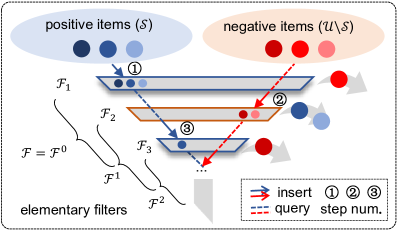
Figure 5. The “$\&\sim$” version shown in Section 4.3.2.

Analysis. Here we analysis the space cost of the new design (denoted as $nf^{CF}({0,\lambda})$ bits) and derive related parameter settings.

Theorem 4.3.

(Space Cost) Suppose an approximate filter costs $C^{\prime}\log 1/\epsilon$ bits per item ($C^{\prime}=\log e=1.44$ for Bloom Filter), then

$$\inf f^{CF}({0,\lambda})=C^{\prime}\log 4e\lambda.$$

Proof.

Our proof is based on a simple observation: Exactly classifying $n$ positive items and $\lambda n$ negative items is equivalent to exactly classifying $\lambda\times n$ positive items and $\lambda\times(1/\lambda)n$ negative items. Formally speaking, we have $f({0,\lambda})=\lambda f({0,1/\lambda})$. We use the above formula to determine the parameter settings, and the following proof is only technically complicated.

W.l.o.g. we let $\lambda\geqslant 1$. According to the chain rule

$$\begin{split}f(0,\lambda)=f(\epsilon,\lambda)+f(0,\epsilon\lambda)=f(\epsilon,\lambda)+\epsilon\lambda f(0,1/(\epsilon\lambda)),\end{split}$$

we have

$$\begin{split}\inf f^{CF}({0,\lambda})/C^{\prime}&=\inf\limits_{\epsilon<1}\left\{\log\frac{1}{\epsilon}+\epsilon\lambda f^{CF}({0,\epsilon\lambda})/C^{\prime}\right\}\\ &=\log\lambda+\inf\limits_{\epsilon<1}\left\{\log\frac{1}{\epsilon\lambda}+\epsilon\lambda f^{CF}({0,\epsilon\lambda})/C^{\prime}\right\}\\ &=\log\lambda+\inf\limits_{x<\lambda}\left\{\log\frac{1}{x}+x\inf f^{CF}({0,\epsilon\lambda})/C^{\prime}\right\}\\ &=\log\lambda+\text{Constant}.\end{split}$$

Since $\inf f^{CF}({0,\epsilon\lambda})$ is derivable, so the right hand side achieves the minimum value when

$$\begin{split}\frac{\mathrm{d}}{\mathrm{d}x}(\log\frac{1}{x}+x\inf f^{CF}({0,\epsilon\lambda})/C^{\prime})=0\end{split}$$

$$\begin{split}\text{Therefore }\begin{cases}\epsilon\lambda=x=1;\\ \inf f^{CF}({0,\epsilon\lambda})=C^{\prime}\log 4e\lambda.\end{cases}\end{split}$$

Actually, according to L’Hôpital’s rule, if

$$\begin{split}&f^{CF}({0,\epsilon\lambda})\equiv C^{\prime}\left(\log\lambda+\log\frac{1}{\delta}+\delta f^{CF}({0,\epsilon\lambda})\right)(\delta<1),\text{ we have}\\ &f^{CF}({0,\epsilon\lambda})=C^{\prime}\left(\log\lambda+\frac{1+\delta}{1-\delta}\log\frac{1}{\delta}\right)\to C^{\prime}\log 4e\lambda(\delta\to 1).\end{split}$$

We show our algorithm in Algorithm 2. ∎

Properties	“&” version	“$\&\sim$” version	Approximate	Exact	Lower bound
($\epsilon=0$)	(Algorithm 1)	(Algorithm 2)	Bloomier	Bloomier
Construction time	$O(|\mathcal{U}|)$	$O(|\mathcal{U}|\log\log n)$	$O(n)$	$O(|\mathcal{U}|)$	Linear
Filter space (bits)	$\approx Cn\log(2e\lambda\ln 2)$	$\approx C^{\prime}n\log 4e\lambda$	$O(n\log\lambda n)$	$\approx C|\mathcal{U}|$	$n(\log\lambda+(\lambda+1)\log(1+1/\lambda))$
Additional space	$\mathchar 266\relax(n\log n)$	/	/	$\mathchar 266\relax(|\mathcal{U}|\log|\mathcal{U}|)$	/

Table 2. Summary of ChainedFilter variants

Input: Universe $\mathcal{U}$ and subset $\mathcal{S}$, $|\mathcal{U}|/|\mathcal{S}|=\lambda>1$.

Output: A filter $\mathcal{F}:\mathcal{U}\mapsto\{0,1\}$ s.t. $\mathcal{F}(e)=1$ iff $e\in S$.

1 Function Construct ($\mathcal{U},\mathcal{S}$):

2 Set $\kappa=\lambda,\delta\in(0,1),\mathcal{S}_{T}=\mathcal{S},\mathcal{S}_{F}=\mathcal{U}\backslash\mathcal{S},i=1.$

3 While $\mathcal{S}_{F}\neq\emptyset:$

4   Construct an approximate filter $\mathcal{F}_{i}$ s.t.

$$\begin{cases}\mathcal{F}_{i}(e)=1,&\forall e\in\mathcal{S}_{T};\\ \mathbb{P}[\mathcal{F}_{i}(e)=0]\leqslant\delta/\kappa,&\forall e\in\mathcal{S}_{F}.\end{cases}$$

5   $\kappa\leftarrow 1/\delta,\mathcal{S}_{T}\leftarrow\mathcal{S}_{F},\mathcal{S}_{F}\leftarrow\{e\in\mathcal{S}_{F}:\mathcal{F}_{i}(e)=0\}.$

6   $i\leftarrow i+1$.

return $\mathcal{F}(\cdot):=\mathcal{F}^{0}(\cdot)$, where $\mathcal{F}^{j}(\cdot):=\mathcal{F}_{j+1}(\cdot)\&\sim\mathcal{F}^{j+1}(\cdot),\forall j\in[0..i-2]$.

Algorithm 2 Exact ChainedFilter (using operator “$\&\sim$”)

Remark 0.

In practice, we can set $\delta=1/2$, round up the space cost of $\mathcal{F}_{1}$ to $C^{\prime}n\lceil\log\lambda/\delta\rceil$ bits, and round up the space cost of $\mathcal{F}_{i}(i\geqslant 2)$ to $C^{\prime}n2\delta^{i-1}\log 1/\delta=C^{\prime}n2^{2-i}$ bits. The total space cost is no more than $C^{\prime}n\log 16\lambda$ bits and the expected query time is $O(1)$. To take a step further, we can replace the last $O(\log n-\log\log n)$ approximate filters with one exact filter whose construction space is $O(n)$, so that we can reduce the number of filters from $O(\log n)$ to $O(\log\log n)$. We summarize the properties of the exact ChainedFilter using operator “&” and “$\&\sim$” in Table 2 (“$/$” means the additional space complexity is no more than the filter space complexity).

5. Applications and Evaluation

$\noindent\bullet$ Experimental Setup: In this section, we implement ChainedFilter and its variants in C++ and Python and equip them with Murmur Hashing (MurmurHash, ) to compute mapped addresses. We evaluate their performance in terms of space usage, speed and accuracy in several applications, including data compressing (Section 5.1, 5.2), classifying (Section 5.3, 5.5), and filtering (Section 5.4). Note that the universe $\mathcal{U}$ may not be the absolute universe. Instead, it can be the set of frequently queried items (Section 5.4). Unless otherwise stated, all item keys are 64-bit pre-generated random integers. All experiments are conducted on a machine with 36 Intel^® Core™ i9-10980XE CPU @ 3.00GHz (576KiB L1 d-cache, 576KiB L1 i-cache, 18MiB L2 cache, 24.8MiB L3 cache) and 128GB DRAM.

$\noindent\bullet$ Our evaluation metrics (with units) are:

(a) Filter space (Mb): The size of the filter measured in million bits (Mb). Additional construction space is not included.

(b) Average construct and query throughput (Mops): The average number of operations per time, measured in million operations per second (Mops). Each experiment was repeated 10 times, and the mean value was recorded to reduce error.

(c) Error rate: The ratio of the number of misclassified (both false positive and false negative) items to the number of all items. We use this metric in Section 5.3.

(d) Tail latency ($\mu s$): The high percentile latency measured in $\mu s$. For example, a P99 latency represents the time cost of an operation which is longer than 99% time costs of all operations. We use this metric in Section 5.4.

(e) False Positive Rate: The ratio of the false positive items to the number of negative items. We use this metric in Section 5.5.

5.1. Static Dictionary

As a warmup, in this part, we use ChainedFilter (”&” version, Algorithm 1) to compactly encode Boolean function $\varphi:\{0,1,...,|\mathcal{U}|\}$ $\mapsto\{0,1\}$ with static support.

5.1.1. Modeling

We regard all $n$ inputs which satisfy $\varphi(\vec{X})=1$ as positive items, and the other $\lambda n$ inputs as negative items. According to the Remark of Theorem 4.1, the exact ChainedFilter requires

$$\begin{split}\frac{C}{1+\lambda}\left(\lfloor\log\lambda\rfloor+1+\frac{\lambda}{2^{\lfloor\log\lambda\rfloor}}\right)|\mathcal{U}|\leqslant\frac{4C}{5\log 5-8}H(\frac{1}{\lambda+1})|\mathcal{U}|\text{ bits,}\end{split}$$

where $C<1.13$ according to the Remark of Section 3. So we have

Corollary 5.1.

When $C<1.13$, ChainedFilter takes at most $4C/(5\log 5-8)=26\%$ space overhead to encode static dictionaries with high probability $1-o(1)$.

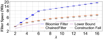
Figure 6. Filter space of the exact Bloomier Filter, ChainedFilter, and the theoretical lower bound. The dotted lines and the dashes represent theoretical and experimental results, respectively. We run each data point for 10 times with different hash seeds. A colored dash indicates a successful construction, while a grey dash indicates the construction fails (you may want to enlarge this figure).

5.1.2. Experiments

We fix $n=1$ million and vary the parameter $\lambda$ from 2 to 16 to compare the filter space, construction throughput and query throughput between ChainedFilter and exact Bloomier Filter. In Figure 6, we find that the experimental space costs correspond well with our theory. Once the allocated space cost is larger than a certain threshold, the filter build processes will succeed with high probability. Specifically, when $\lambda=16$, ChainedFilter costs 64% less space than exact Bloomier Filter. In Figure 7 (a), we discover that the construction throughput of exact Bloomier Filter decreases as $\lambda$ increases, whereas that of ChainedFilter increases as $\lambda$ increases. This is because although a larger $\lambda$ leads to a worse locality, the throughput bottle neck of ChainedFilter is from the space cost of exact Bloomier Filter, which fluctuates between $2Cn$ (when $\lambda=2,4,8,16$) and $3Cn$. Therefore, the amortized throughput of each item of ChainedFilter increases, and it even surges from the case of $\lambda=2^{i}-1$ to the case of $\lambda=2^{i}(i=2,3,4,...)$. Specifically, when $\lambda=16$, the construction throughput of ChainedFilter is 407% higher than that of Exact Bloomier Filter. In Figure 7 (b), we observe that the query throughput of ChainedFilter shows the same phenomenon. This is because only the positive items and the false positive items require the lookup of the second stage filter. Specifically, when $\lambda=16$, the query throughput of ChainedFilter is 103% higher than that of Exact Bloomier Filter.

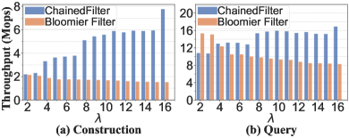
Figure 7. Average construction and query throughput.

5.2. Random Access Huffman Coding

In this part, we apply ChainedFilter to lossless data compression.

5.2.1. Background

In information theory, Huffman Coding (huffman1952method, ) is an optimal prefix coding technique for lossless data compression. Given the possibility of occurrence of all kinds of symbols $\vec{p}:=(p_{1},p_{2},...)$, the Huffman’s algorithm generates a variable-length code table, namely Huffman Tree, which assigns an $l_{i}-$bit prefix code for the $i$-th symbol. The literature shows that the average code length $\overline{{L}}_{\mathrm{Huff}}:=\sum l_{i}p_{i}$ satisfies

$$H(\vec{p})\leqslant\overline{{L}}_{\mathrm{Huff}}<H(\vec{p})+1,\text{ where }H(\vec{p}):=-\sum\limits_{i}p_{i}\log p_{i}.$$

Although Huffman’s algorithm is optimal for separate symbols, it has certain limitations: (1) Compression ratio. Unlike arithmetic coding or ANS (duda2013asymmetric, ), $\overline{{L}}_{\mathrm{Huff}}$ may not approach the entropy $H(\vec{p})$ arbitrarily. For example, if we have a string consisting of one character ‘a’ and $1023$ character ‘b’. The Huffman’s algorithm will cost $1024$ bits to encode them, but the least space cost is only 10 bits since we can simply record the address of ‘a’. (2) Decoding order. The Huffman’s algorithm does not support random memory access of data. (3) Confidentiality. Attackers with prior knowledge of the character’s frequency $\vec{p}$ can decipher the unencrypted Huffman Tree. (4) Robustness. In Huffman Code, small interference (bit flip or loss) may cause it to fail to recognize the starting position of characters, resulting in decoding failure. Some alternative approaches can partially address these problems. For example, (1) blocking some symbols can increase the compression ratio at the expense of the Huffman Tree’s complexity; (2) Encoding the Huffman Code into a perfect hash table can support random access at the expense of space overhead (hreinsson2009storing, ); (3) Encryption and (4) error correcting code may increase the confidentiality and robustness at the expense of time and space overhead.

5.2.2. Modeling

ChainedFilter (”&” version, Algorithm 1) can overcome the four limitations simultaneously. Given the Huffman Tree based on the probability vector $\vec{p}$, we encode every character’s address paired with its Huffman Code into ChainedFilter. Specifically, for the $i$-th character in the data with Huffman Code $\vec{v}=(v_{1},v_{2}...,v_{k})\in\{0,1\}^{k}$, we encode $(\text{key}=(i,j),\text{value}=v_{j}),j\in[1..k]$ into ChainedFilter. To query the $i$-th character, we can query $\text{key}=(i,1),(i,2)...$ until the leaf node of the Huffman Tree.

For example, to compress a string ”ab$\backslash$0” with its Huffman Tree (‘a’$\to$00, ‘b’$\to$ 01, ‘$\backslash$0’$\to$1), we can encode the negative items $(1,1),$ $(1,2),$ $(2,1)$ and the positive items $(2,2),(3,1)$ into ChainedFilter. To query, say, the second character, we first query key $=(2,1)$ and find that it is negative, and then query key$=(2,2)$ and find that it is positive. Therefore, we know that the second character whose Huffman Code is “01” is ‘b’.

Our algorithm has random access property, high confidentiality (as long as the hash seed is secure), and high robustness. In Theorem 5.1, we prove that ChainedFilter optimizes the worst-case compression ratio performance as well.

Theorem 5.1.

The average code length of our algorithm, denoted as $\overline{{L}}_{\mathrm{ours}}$, satisfies $H(\vec{p})<\overline{{L}}_{\mathrm{ours}}<H(\vec{p})+0.22$ with high probability $1-o(1)$.

Proof.

We only prove the right inequality by mathematical induction. For convenience, we define constant $C_{0}:=0.22$. First, if the Huffman Tree has only two leaf nodes, according to the Remark of Theorem 4.1, we have

$$\begin{split}\overline{L}_{\mathrm{ours}}&\leqslant\frac{C}{1+\lambda}\left(\lfloor\log\lambda\rfloor+1+\frac{\lambda}{2^{\lfloor\log\lambda\rfloor}}\right)\\ &\leqslant H(p)+C+\frac{2}{3}-\log 3<H(p)+C_{0}.\end{split}$$

Consider there are two Huffman Trees that satisfy the above inequality. We combine them into a larger Huffman Tree with weights $q$ and ($1-q$), respectively. Since the number of layers is increased by one, we have

$$\begin{split}\overline{L}&{}_{\mathrm{ours}}=\sum\limits_{i}qp_{1i}(l_{1i}+1)+\sum\limits_{i}(1-q)p_{2i}(l_{2i}+1)\\ &\leqslant qH(\vec{p}_{1})+(1-q)H(\vec{p}_{2})+1+C_{0}\\ &=-\sum\limits_{i}qp_{1i}\log qp_{1i}-\sum\limits_{i}(1-q)p_{2i}\log(1-q)p_{2i}\\ &\quad+q\sum\limits_{i}\log q+(1-q)\sum\limits_{i}\log(1-q)+1+C_{0}\\ &=H(\vec{p})-(H(q)-1)+C_{0}<H(\vec{p})+C_{0}.\end{split}$$

So $\overline{L}_{\mathrm{ours}}<H(\vec{p})+C_{0}$ holds for all Huffman Trees. ∎

Remark 0.

Theorem 5.1 demonstrates that our algorithm has a tighter upper bound (0.22 bit per item) on space overhead than the standard Huffman’s algorithm (1 bit per item). This is particularly advantageous when the data is highly skewed or sparse. However, one drawback of ChainedFilter is its poor spacial locality, which limits its throughput in hierarchical memory systems. To compensate this drawback, we can enable the first and the second stage filters to share the same mapped addresses, as suggested in (reviriego2021approximate, ). The optimized version uses a $Cn\lceil\log\lambda\rceil$-bit approximate Bloomier Filter (with less than $n$ false positive items) and a $2Cn$-bit exact Bloomier Filter, and every $(\lceil\log\lambda\rceil+2)$ bits are organized as a block. With this optimization, each item has $j=3$ common mapped blocks shared by both of the first and the second stages, making it possible to access its value within $j$ memory accesses.

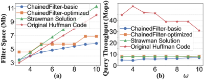
Figure 8. Filter space and query throughput of random access Huffman coding algorithms.

5.2.3. Experiments

We synthesize eight datasets of strings whose characters’ occurrence obeys an exponential distribution with parameter $\omega=3,4,...,10,$ respectively. We fix the number of positive items to 1 million, generate the Huffman Code for each string, and encoding the Huffman Code using ChainedFilter and its optimized version (Remark of Theorem 5.1). To provide a strawman solution, we encode the Huffman Code into an exact Bloomier Filter and record its filter space and query throughput. For reference, we also evaluate the performance of raw Huffman Coding, but present its sequential decoding throughput rather than random decoding throughput (because it does not support random access). The experimental results are shown in Figure 8, we find that ChainedFilter performs better as $\omega$ grows. When $\omega=10$, the basic and the optimized versions of ChainedFilter saves 48.3% and 39.2% of the filter space compared to the strawman solution, while their query throughput is only 15.5% and 1.17% slower.

5.3. Self-Adaptive Hashing

In this part, we use ChainedFilter to reduce the number of memory accesses required for Cuckoo Hashing (pagh2004cuckoo, ).

5.3.1. Background

Serving as a hash predictor, ChainedFilter reduces unnecessary memory accesses for multiple-choice hashing, which take around $100ns$ for DRAM and $\approx 150\mu s$ for NAND SSD. Instead, it requires only a few fast (around $10$ ns) in-cache lookups.

Based on ”the power of two random choices” (mitzenmacher2001power, ), Cuckoo Hashing consists of two hash tables $T_{1}[1..M]$ and $T_{2}[1..M]$, allowing an item $e$ to have two potential mapping locations $T_{1}[\mathrm{h}_{1}(e)]$ and $T_{2}[\mathrm{h}_{2}(e)]$. Each item can only occupy one location at a time, but can swap between the two if its prior location is taken. To insert an item $e$, we first attempt to place it into $T_{1}[\mathrm{h}_{1}(e)]$. If $T_{1}[\mathrm{h}_{1}(e)]$ is already occupied by another item $e^{\prime}$, we evict $e^{\prime}$ and reinsert it into $T_{2}[\mathrm{h}_{2}(e^{\prime})]$. We repeat this process until all items stabilize. If this is impossible, we reconstruct the cuckoo hash table with a new hash seed. The literature shows that the insertion failure probability is $O(1/M)$ when the occupancy (load factor $r$) is less than $1/2-\varepsilon$. However, to query an item, we often check both of the two hash tables, which can result in significant latency penalties.

A well known solution to reduce the number of memory accesses for Cuckoo Hashing is to use a pre-filter, such as a Bloom Filter (bloom1970space, ) or Counting Bloom Filter (fan2000summary, ), to predict the mapped locations of each item. However, false predictions by the pre-filter can cause additional memory accesses. To address this problem, EMOMA (pontarelli2018emoma, ) adds a 1(block):1(bucket) pre-Counting Block Bloom Filter that corresponds to the first hash table, and locks certain items in the second hash table to prevent movements that may cause false positives. This creates an always-exact hash predictor that supports line-rate processing (e.g. in programmable switches or FPGAs) at the expense of complex insertion process and space overhead.

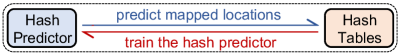
Figure 9. The concept of the self-adaptive hashing.

5.3.2. Modeling

Instead of supporting absolute exact matches, we use ChainedFilter (”$\&\sim$” version, Algorithm 2) as a pre-filter to predict the mapped locations with best effort. Our key idea is to let false predictions train the predictor to reduce errors (Figure 9). Specifically, we regard items in the first hash table as negative and those in the second hash table as positive. To query an item $e$, we ask ChainedFilter for the predicted location. If the prediction is incorrect, we adjust ChainedFilter by flipping the mapped bits in $\mathcal{F}_{1},\mathcal{F}_{2},\mathcal{F}_{3},...$ to 1 until ChainedFilter can accurately predict the locations of $e$. In the Remark of Theorem 4.3, we have proved that the error rate will ultimately converge to zero as long as the space cost of is greater than $C^{\prime}n\left(\log\lambda-((1+\delta)/(1-\delta))\log\delta\right)$. Next we show how to choose the negative-positive ratio $\lambda$.

Theorem 5.2.

Given the expected number of items $|\mathcal{U}|$ and the number of buckets in the Cuckoo hash table, $2M$, we define $r:=|\mathcal{U}|/2M<1/2-\varepsilon$ is the load factor. Then we have

$$\lambda=\left(\frac{2r}{1-e^{-2r}}-1\right)^{-1}+o(1).$$

Proof.

Let $\eta$ be the number of negative items (items in the first hash table). A new item can either insert into an empty location in the first hash table, increasing $\eta$ by one, or evict an old item with probability $\eta/M$ (assuming no insertion failures). This problem can be reformulated as the well-known coupon collector’s problem, where $M$ is the number of coupons and $\eta$ is the number of draws. Therefore, we have

$$\begin{split}2r=\sum\limits_{l=M-\eta}^{M}\frac{1}{l}+o&(1)=\int\limits_{1-\eta/M}^{1}\frac{1}{x}\mathrm{d}x+o(1)=\ln\left(1-\frac{\eta}{M}\right)+o(1)\\ &\Rightarrow\lambda:=\frac{\eta}{2rM-\eta}=\left(\frac{2r}{1-e^{-2r}}-1\right)^{-1}+o(1).\end{split}$$

∎

Remark 0.

According to Theorem 5.2 and the Remark of Section 4.3.2, when $\delta=1/2$, ChainedFilter incurs a space cost of no more than $C^{\prime}n\log 16\lambda=2C^{\prime}r/(\lambda+1)\log 16\lambda\cdot M$ bits. In contrast, the Counting Block Bloom Filter of EMOMA (pontarelli2018emoma, ) costs $8M$ bits if every block has two 4-bit counters. In the following experiments, we fix the Cuckoo hash table size $2M$ to 1 million. Table 3 shows the space cost (measured in Mb) of ChainedFilter ($\delta=1/2$) and EMOMA when $r\in[0.1,0.4]$ (for reasonable comparison, the space cost of Bloom Filter equals to that of EMOMA). We observe that ChainedFilter is much more space-efficient: it saves $76.7\%$ (r=0.4) $\sim$ $99.75\%$ (r=0.1) space of EMOMA to predict exact locations.

	0.10	0.15	0.20	0.25	0.30	0.35	0.40
EMOMA	4.00	4.00	4.00	4.00	4.00	4.00	4.00
ChainedFilter	0.10	0.20	0.32	0.45	0.60	0.76	0.93

Table 3. Filter space of EMOMA and ChainedFilter.

5.3.3. Experiments

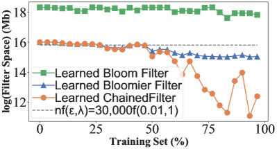
Figure 13. Filter space in bits ($\log$ scale) of Learned Bloom Filter, Learned Bloomier Filter and Learned ChainedFilter.

In the first experiment, we show that although ChainedFilter may not initially predict the mapped locations absolutely exactly, its error rate decreases exponentially and can quickly converge to zero. To verify this, we set $r=0.4$ and query all items in order for $R$ rounds to train the ChainedFilter and show the change in error rate in Figure 13 (a). We find that only $0.34\%$ items are wrongly predicted after three rounds of training, and all items are exactly predicted after seven rounds of training, resulting in a reduction of $(\lambda+1)^{-1}|_{r=0.4}=31\%$ external memory access for Cuckoo Hashing. To further accelerate the training process, we insert all items of the $\lfloor\log\log n\rfloor=4$-th layer $\mathcal{F}_{4}$ into an Othello hash table (yu2018memory, ) according to the Remark of Section 4.3.2, so that the training process can be completed in four rounds (“ChainedFilter-optimized” in Figure 13). In the second experiment, we use keys of length 36 bytes and values of length 64 bytes and compare the throughput of raw Cuckoo Hashing, Cuckoo Hashing with ChainedFilter, with EMOMA, and with Bloom Filter (Figure 13 (b)). We find that although ChainedFilter uses only $23.3\%$ of the filter space of EMOMA, its average construction and query throughput is 17% and 41% faster, respectively. It is interesting to note that both Cuckoo Hashing with EMOMA and Cuckoo Hashing with Bloom Filter exhibit slower query throughput compared to raw Cuckoo Hashing, possibly due to their higher hash computation overhead.

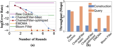
Figure 10. Error rate and throughput of raw Cuckoo Hashing, Cuckoo Hashing with ChainedFilter (0.93Mb), with EMOMA (4Mb), and with Bloom Filter (4Mb).

5.4. Point Query for LSM-Tree

In the final application, we utilize ChainedFilter to reduce the tail point query latency of LSM-Tree.

5.4.1. Background

LSM-Tree (short for log-structured merge-tree) is a storage system for high write-throughput of key-value pairs. It uses an in-memory data structure called memtable to buffer all updates until it is full, and then flushes the contents into the persistent storage as a sorted run through a process called minor compaction. However, since the sorted runs may have overlapping key ranges, LSM-Tree has to check all of them for a point query, which can result in poor query performance. To address this problem, LSM-Tree uses a hierarchical merging process called major compaction to merge sorted runs. In tiered major compaction, the LSM-Tree is organized as a sequence of levels, and the number of runs in each level is bounded by a threshold $T$. If the number achieves the threshold, the compaction process is triggered to merge all $T$ sorted runs a new sorted run (SSTable) in the next level. To further speed up point queries, each SSTable typically has an approximate filter, such as a Bloom Filter, to skip most non-existing items. However, since the approximate filter has false positives, in the worst case, a point query still needs to check all SSTables, resulting in poor tail point query latency.

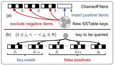
Figure 11. ChainedFilter (“& version”) for LSM-Tree. Note that the second stage part must be a dynamic filter.

5.4.2. Modeling

To reduce the latency, we replace every approximate filter with a dynamic exact ChainedFilter (“&” version, Algorithm 1 and Section 4.3.1). Suppose there are $N$ SSTables in one level, our goal is to reduce the worst case additional SSTable search time from $N$ to 1 (whether or not there are repeating items). Our key idea is, for ChainedFilter of the $i$-th SSTable in this level, we regard all keys in the $i$-th SSTable as positive items, and regard all other keys in the $(i+1),(i+2),...,N$-th SSTables (but not in the $i$-th SSTable) as negative items (Figure 11 (a)). In this way, an exact ChainedFilter says “yes” only when (1) the queried key is in its corresponding SSTable, (2) the queried key is not in the subsequent $(i+1),(i+2),...,N$-th SSTables in the same level (otherwise the key must be excluded when the later SSTables are formed). Consider the case where the $j_{1}<j_{2}<...<j_{k}$-th ChainedFilters report “yes”. Our strategy is to check the corresponding SSTables in order until we find a false positive SSTable (note that the item keys are repeatable). Once we detect that the $j_{l}$-th ChainedFilter’s result is a false positive, we can assert that all the $j_{l+1},j_{l+2},...,j_{k}$-th ChainedFilter’s results are false positives as well (Figure 11 (b)). Therefore, the number of additional SSTable searches in this level is no more than one.

5.4.3. Experiments

We measure the tail point query latency of our approach in RocksDB database (dong2021rocksdb, ) by replacing the built-in Bloom Filter with the ChainedFilter. To simplify the implementation, we let all SSTables stay in the first level (L0) and use the default 64MB write buffer size. We reuse the built-in Bloom Filter as the first stage of ChainedFilter, but additionally implement an Othello hash table as the dynamic second stage filter. When creating a new SSTable after a compaction, we generate the Bloom Filter as what RocksDB does, but additionally query its keys in prior SSTables in the same level and update the false positive SSTables’ ChainedFilters by including the false positive items into the second stage filter (Figure 11 (a)). When querying an item, we check the positive SSTables (whose Bloom Filter reports “yes”) in order. Once we find a false positive one, we can assert that all later possible SSTables are false positives (Figure 11 (b)).

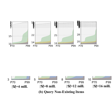
Figure 12. Tail point query latency in RocksDB.

Figure 12 demonstrates that ChainedFilter can significantly reduce the tail point query latency of LSM-Tree. We generate items with distinct 36-Byte random keys and 64-Byte values and vary the number of items $|\mathcal{U}|$ from 4 million (400MB data, 7 SSTables in total) to 16 million (1.6GB data, 30 SSTables in total). The filter space of ChainedFilter just allows it to exactly classify positive and negative items. We use RocksDB with only Bloom Filters with the $0\times,1\times,\text{ and }2\times$ filter space as the comparison algorithm (“$0\times$” means no filter). In Figure 12 (a), we show the tail latency of querying existing items. Let us consider the “$|\mathcal{U}|$=16 mill.” sub-figure as an example. The green area in the figure shows the tail point query latency using only built-in Bloom Filter which costs the same space as ChainedFilter. The P0-P77, P77-P95, and P95-P99 tail latency approximately represents the query latency with zero, one, and more than one false positive SSTable reads. In the worst case, with many false positive SSTable reads, the P99 tail point query latency is about $31\mu s$. In contrast, as shown in the blue area, the query process using ChainedFilter has no false positive when querying existing items, so the tail latency remains under $20\mu s$, which is 36% lower. In Figure 12 (b), we show the tail latency of querying non-existing items. We find that when $|\mathcal{U}|$ is 16 million, the latency with ChainedFilter gradually increases. This is because the latency is not only determined by the number of false positive SSTables, but is also influenced by the index of the false positive ChainedFilter. For example, if the first SSTable reports a false positive, the algorithm can quickly return, and thus the overall latency may be even lower than $12\mu s$. However, if the 30-th SSTable is the first one to report false positive, the overall latency will be more than $18\mu s$.

5.5. Learned Filter

In this part, we use ChainedFilter to reduce the false positive rate of Learned Filters.

5.5.1. Background

Although our space lower bound (Section 2.2) assumes that the positive items are randomly drawn from the universe, further compression can be achieved when the items follow a specific data distribution. Learned Filters (kraska2018case, ; mitzenmacher2018model, ; liu2020stable, ; dai2020adaptive, ) incorporate a continuous function, such as an RNN model, in front of the filter structure to capture the data distribution. When querying an item, if the continuous function outputs “yes”, the Learned Filter immediately reports true. However, when the continuous function outputs “no”, the item is sent to a backup Bloom Filter to eliminate false negatives. In the learned filter structure, both the learning model and the backup filter may introduce false positives, but in some cases, the overall false positive rate even decreases.

5.5.2. Experiments

Extending the chain rule (Theorem 2.2) to general membership problems with different data distributions is an intriguing problem. Since we haven’t derive an elegant theory at this moment, we empirically replace the backup Bloom Filter / Bloomier Filter with our ChainedFilter (“&” version) to show the experimental improvements. We refer to the open-source code of the learned Bloom Filter and the dataset on GitHub (LearnedFilter, ). The dataset has 30,000 positive (good) and 30,000 negative (bad) websites evaluated by users. In this experiment, we randomly select different proportions (ranging from $0\%$ to $100\%$) of data to train the RNN model. Generally, the model’s generalization ability improves as the amount of training data increases. Experimental results show that when we fix the overall false positive rate at 0.01, the filter space of Learned ChainedFilter can be up to 99.1% lower than that of Learned Bloom Filter and 96.2% lower than $nf(\epsilon,\lambda)$ (the space lower bound without considering data distribution).

6. Related Work

Filter algorithms are the foundation of many important problems (wu2021elastic, ; 9944968, ; stingysketch, ; li2023ladderfilter, ; guo2023sketchpolymer, ; Rencoder, ; namkung2022sketchlib, ; li2023steadysketch, ; fan2022evolutionary, ; namkung2023sketchovsky, ; liu2023hypercalm, ) and have been well studied. In this section, we introduce more membership filters that may work as our elementary filters.

6.1. Approximate Membership Filters

Approximate filters originated with Bloom Filter (bloom1970space, ) in 1970. A Bloom Filter is a bitmap of size $m$ where every one of $n$ positive items is mapped using $k$ independent hash functions. To insert an item, we set all mapped positions to one; To query an item, we check whether all mapped positions are one, and report positive iff they are. A Bloom Filter satisfies one-sided error: a query is either “definitely not” (no false negative) or “probably yes” (small false positive). The false positive rate depends on the space cost

$$\epsilon=\left(1-\left(1-\frac{1}{m}\right)^{nk}\right)^{k}\approx\left(1-e^{-\frac{nk}{m}}\right)^{k}\Rightarrow m\geqslant\frac{n\log 1/\epsilon}{\ln 2}.$$

In 1978, (carter1978exact, ) gave the tight space lower bound ($\log 1/\epsilon+o(1)$ bits per item) for approximate filters, which means the Bloom Filter wastes no more than $1/\ln 2-1=44\%$ space. In 2010, (lovett2013space, ) gave the space lower bound $C(\epsilon)\log 1/\epsilon$ bits per item for dynamic approximate data structures, where $C(\epsilon)>1$ depends only on $\epsilon$. Many later works have emerged to reduce the space overhead of Bloom Filter. Cuckoo Filter (2014) (fan2014cuckoo, ) borrows the concept from Cuckoo Hashing (Background of Section 5.3) and uses fingerprints for approximate classification. It maps an item $e$ to two buckets $h(e)$ and $(h(e)\oplus f(e))$ in one hash table, and shows that the load factor can be up to 95% if the buckets have four slots. Therefore, the space cost drops to $1.05(2+\log 1/\epsilon)$ bits per item. Inspired by Bloomier filter and the peeling theory, XOR Filter (2019) (graf2020xor, ) and Binary Fuse Filter (2022) (graf2022binary, ) achieves a space cost of $C\log 1/\epsilon$ bits per item for static membership query (Remark of Section 3). In fact, a more compact space cost ($(1+o(1))\log 1/\epsilon$ bits per item) is given by (dietzfelbinger2008succinct, ) (2008) and (porat2009optimal, ) (2009) for static membership query if we allow a more complex implementation.

6.2. Exact Membership Filters

One type of exact filters builds upon perfect hashing (majewski1996family, ). The Bloomier Filter (chazelle2004bloomier, ; charles2008bloomier, ) (2004) is a milestone which requires $1.23$ bits per item (the theoretical result is excerpted from IBLT (2011) (goodrich2011invertible, )). According to (walzer2021peeling, ) (2021), this constant can be optimized to close to 1 (Remark of Section 3). In fact, a more compact space cost of $(1+o(1))$ bits per item is achievable if a more complex implementation is allowed (dietzfelbinger2008succinct, ; porat2009optimal, ). Othello Hashing (yu2018memory, ) (2016) and Coloring Embedder (tong2019coloring, ) (2021) provide dynamic perfect hashing designs with $O(1)$ bits per item. However, they both need additional structures with $\mathchar 266\relax(n\log n)$ space for construction and update.

Another one type of exact filters is called “dictionaries”. In 1984, (fredman1984storing, ) described a general constant-time hashing scheme (FKS dictionary) with a space complexity of $O(n)$ words (not bits). In 1994, researchers designed an static exact filter with a space complexity of $O(B)$ (brodnik1994membership, ) (they later improved to $B(1+O(1/\log\log\log|\mathcal{U}|))$ (brodnik1999membership, ) in 1999) for static dictionary, where $B:=\lceil\log\binom{|\mathcal{U}|}{n}\rceil$ is the lower bound for static membership problems (carter1978exact, ). In 2001, the space complexity is optimized to nearly optimal ($B+O(\log\log(|\mathcal{U}|))+o(n)$ bits) (pagh2001low, ). In 2010, (arbitman2010backyard, ) proofs the lower bound $(1+o(1))B$ also holds for dynamic exact membership filters. Nowadays, the research on exact membership problems is still on going (bercea2020space, ).

In the end, we list some other membership filters satisfying special properties. In 2005, (pagh2005optimal, ) started considers dynamic general membership problems and designed a membership filter with a space complexity of $((1+o(1))n\log 1/\epsilon+O(n+\log|\mathcal{U}|)$ bits for arbitrary $\epsilon$ and $\lambda$. Since 2018, researchers have creatively introduced machine learning methodology to construct Learned Bloom Filters (kraska2018case, ; mitzenmacher2018model, ; liu2020stable, ; dai2020adaptive, ), or add pre-filters to construct membership algorithms (reviriego2021approximate, ), which are more accurate than the original Bloom Filter.

7. Conclusion

In this paper, we present a lossless factorization theorem, namely chain rule, for solving general membership query problems. Based on this theorem, we propose a simple yet space-efficient filter framework called ChainedFilter and apply it to various applications. Both theoretical and experimental results show that the ChainedFilter outperforms its elementary filters. We believe our chain rule can inspire more innovative works, and our ChainedFilter can be used in more practical applications.

References

- [1] Sasu Tarkoma, Christian Esteve Rothenberg, and Eemil Lagerspetz. Theory and practice of bloom filters for distributed systems. IEEE Communications Surveys & Tutorials, 14(1):131–155, 2011.
- [2] Andrei Broder and Michael Mitzenmacher. Network applications of bloom filters: A survey. Internet mathematics, 1(4):485–509, 2004.
- [3] Shahabeddin Geravand and Mahmood Ahmadi. Bloom filter applications in network security: A state-of-the-art survey. Computer Networks, 57(18):4047–4064, 2013.
- [4] Fay Chang, Jeffrey Dean, Sanjay Ghemawat, Wilson C Hsieh, Deborah A Wallach, Mike Burrows, Tushar Chandra, Andrew Fikes, and Robert E Gruber. Bigtable: A distributed storage system for structured data. ACM Transactions on Computer Systems (TOCS), 26(2):1–26, 2008.
- [5] Niv Dayan, Manos Athanassoulis, and Stratos Idreos. Optimal bloom filters and adaptive merging for lsm-trees. ACM Transactions on Database Systems (TODS), 43(4):1–48, 2018.
- [6] Yoshinori Matsunobu, Siying Dong, and Herman Lee. Myrocks: Lsm-tree database storage engine serving facebook’s social graph. Proceedings of the VLDB Endowment, 13(12):3217–3230, 2020.
- [7] Sarang Dharmapurikar, Haoyu Song, Jonathan Turner, and John Lockwood. Fast packet classification using bloom filters. In Proceedings of the 2006 ACM/IEEE symposium on Architecture for networking and communications systems, pages 61–70, 2006.
- [8] Dan Li, Henggang Cui, Yan Hu, Yong Xia, and Xin Wang. Scalable data center multicast using multi-class bloom filter. In 2011 19th IEEE international conference on network protocols, pages 266–275. IEEE, 2011.
- [9] Pedro Reviriego, Jorge Martínez, David Larrabeiti, and Salvatore Pontarelli. Cuckoo filters and bloom filters: Comparison and application to packet classification. IEEE Transactions on Network and Service Management, 17(4):2690–2701, 2020.
- [10] Michael T Goodrich and Michael Mitzenmacher. Invertible bloom lookup tables. In 2011 49th Annual Allerton Conference on Communication, Control, and Computing (Allerton), pages 792–799. IEEE, 2011.
- [11] A Pinar Ozisik, Gavin Andresen, Brian N Levine, Darren Tapp, George Bissias, and Sunny Katkuri. Graphene: efficient interactive set reconciliation applied to blockchain propagation. In Proceedings of the ACM Special Interest Group on Data Communication, pages 303–317. 2019.
- [12] Muhammad Anas Imtiaz, David Starobinski, Ari Trachtenberg, and Nabeel Younis. Churn in the bitcoin network: Characterization and impact. In 2019 IEEE International Conference on Blockchain and Cryptocurrency (ICBC), pages 431–439. IEEE, 2019.
- [13] Larry Carter, Robert Floyd, John Gill, George Markowsky, and Mark Wegman. Exact and approximate membership testers. In Proceedings of the tenth annual ACM symposium on Theory of computing, pages 59–65, 1978.
- [14] Bin Fan, Dave G Andersen, Michael Kaminsky, and Michael D Mitzenmacher. Cuckoo filter: Practically better than bloom. In Proceedings of the 10th ACM International on Conference on emerging Networking Experiments and Technologies, pages 75–88, 2014.
- [15] Siying Dong, Andrew Kryczka, Yanqin Jin, and Michael Stumm. Rocksdb: Evolution of development priorities in a key-value store serving large-scale applications. ACM Transactions on Storage (TOS), 17(4):1–32, 2021.
- [16] Tim Kraska, Alex Beutel, Ed H Chi, Jeffrey Dean, and Neoklis Polyzotis. The case for learned index structures. In Proceedings of the 2018 international conference on management of data, pages 489–504, 2018.
- [17] Michael Mitzenmacher. A model for learned bloom filters and optimizing by sandwiching. Advances in Neural Information Processing Systems, 31, 2018.
- [18] Qiyu Liu, Libin Zheng, Yanyan Shen, and Lei Chen. Stable learned bloom filters for data streams. Proceedings of the VLDB Endowment, 13(12):2355–2367, 2020.
- [19] Zhenwei Dai and Anshumali Shrivastava. Adaptive learned bloom filter (ada-bf): efficient utilization of the classifier with application to real-time information filtering on the web. Advances in Neural Information Processing Systems, 33:11700–11710, 2020.
- [20] The open source code of chainedfilter. https://github.com/ChainedFilter.
- [21] Bernard Chazelle, Joe Kilian, Ronitt Rubinfeld, and Ayellet Tal. The bloomier filter: an efficient data structure for static support lookup tables. In Proceedings of the fifteenth annual ACM-SIAM symposium on Discrete algorithms, pages 30–39. Citeseer, 2004.
- [22] Denis Charles and Kumar Chellapilla. Bloomier filters: A second look. In Algorithms-ESA 2008: 16th Annual European Symposium, Karlsruhe, Germany, September 15-17, 2008. Proceedings 16, pages 259–270. Springer, 2008.
- [23] Thomas Mueller Graf and Daniel Lemire. Xor filters: Faster and smaller than bloom and cuckoo filters. Journal of Experimental Algorithmics (JEA), 25:1–16, 2020.
- [24] Thomas Mueller Graf and Daniel Lemire. Binary fuse filters: Fast and smaller than xor filters. Journal of Experimental Algorithmics (JEA), 27(1):1–15, 2022.
- [25] Stefan Walzer. Peeling close to the orientability threshold–spatial coupling in hashing-based data structures. In Proceedings of the 2021 ACM-SIAM Symposium on Discrete Algorithms (SODA), pages 2194–2211. SIAM, 2021.
- [26] Ye Yu, Djamal Belazzougui, Chen Qian, and Qin Zhang. Memory-efficient and ultra-fast network lookup and forwarding using othello hashing. IEEE/ACM Transactions on Networking, 26(3):1151–1164, 2018.
- [27] Yang Tong, Dongsheng Yang, Jie Jiang, Siang Gao, Bin Cui, Lei Shi, and Xiaoming Li. Coloring embedder: A memory efficient data structure for answering multi-set query. In 2019 IEEE 35th International Conference on Data Engineering (ICDE), pages 1142–1153. IEEE, 2019.
- [28] Burton H Bloom. Space/time trade-offs in hash coding with allowable errors. Communications of the ACM, 13(7):422–426, 1970.
- [29] Yuriy Arbitman, Moni Naor, and Gil Segev. Backyard cuckoo hashing: Constant worst-case operations with a succinct representation. In 2010 IEEE 51st Annual symposium on foundations of computer science, pages 787–796. IEEE, 2010.
- [30] Shachar Lovett and Ely Porat. A space lower bound for dynamic approximate membership data structures. SIAM Journal on Computing, 42(6):2182–2196, 2013.
- [31] Murmur hashing source code. https://github.com/aappleby/smhasher/blob/master/src/MurmurHash3.cpp.
- [32] David A Huffman. A method for the construction of minimum-redundancy codes. Proceedings of the IRE, 40(9):1098–1101, 1952.
- [33] Jarek Duda. Asymmetric numeral systems: entropy coding combining speed of huffman coding with compression rate of arithmetic coding. arXiv preprint arXiv:1311.2540, 2013.
- [34] Jóhannes B Hreinsson, Morten Krøyer, and Rasmus Pagh. Storing a compressed function with constant time access. In Algorithms-ESA 2009: 17th Annual European Symposium, Copenhagen, Denmark, September 7-9, 2009. Proceedings 17, pages 730–741. Springer, 2009.
- [35] Pedro Reviriego, Alfonso Sánchez-Macián, Stefan Walzer, and Peter C Dillinger. Approximate membership query filters with a false positive free set. arXiv preprint arXiv:2111.06856, 2021.
- [36] Rasmus Pagh and Flemming Friche Rodler. Cuckoo hashing. Journal of Algorithms, 51(2):122–144, 2004.
- [37] Michael Mitzenmacher. The power of two choices in randomized load balancing. IEEE Transactions on Parallel and Distributed Systems, 12(10):1094–1104, 2001.
- [38] Udi Manber and Sun Wu. An algorithm for approximate membership checking with application to password security. Information Processing Letters, 50(4):191–197, 1994.
- [39] Li Fan, Pei Cao, Jussara Almeida, and Andrei Z Broder. Summary cache: a scalable wide-area web cache sharing protocol. IEEE/ACM transactions on networking, 8(3):281–293, 2000.
- [40] Salvatore Pontarelli, Pedro Reviriego, and Michael Mitzenmacher. Emoma: Exact match in one memory access. IEEE Transactions on Knowledge and Data Engineering, 30(11):2120–2133, 2018.
- [41] Yoav Freund, Robert Schapire, and Naoki Abe. A short introduction to boosting. Journal-Japanese Society For Artificial Intelligence, 14(771-780):1612, 1999.
- [42] The open source code of learned filter. https://github.com/karthikeya20/Learned-Bloom-Filters.
- [43] Yuhan Wu, Jintao He, Shen Yan, Jianyu Wu, Tong Yang, Olivier Ruas, Gong Zhang, and Bin Cui. Elastic bloom filter: deletable and expandable filter using elastic fingerprints. IEEE Transactions on Computers, 71(4):984–991, 2021.
- [44] Zhuochen Fan, Yubo Zhang, Siyuan Dong, Yi Zhou, Fangyi Liu, Tong Yang, Steve Uhlig, and Bin Cui. Hoppingsketch: More accurate temporal membership query and frequency query. IEEE Transactions on Knowledge and Data Engineering, 35(9):9067–9072, 2023.
- [45] Haoyu Li, Qizhi Chen, Yixin Zhang, Tong Yang, and Bin Cui. Stingy sketch: A sketch framework for accurate and fast frequency estimation. Proc. VLDB Endow., 15(7):1426–1438, mar 2022.
- [46] Yuanpeng Li, Feiyu Wang, Xiang Yu, Yilong Yang, Kaicheng Yang, Tong Yang, Zhuo Ma, Bin Cui, and Steve Uhlig. Ladderfilter: Filtering infrequent items with small memory and time overhead. Proceedings of the ACM on Management of Data, 1(1):1–21, 2023.
- [47] Jiarui Guo, Yisen Hong, Yuhan Wu, Yunfei Liu, Tong Yang, and Bin Cui. Sketchpolymer: Estimate per-item tail quantile using one sketch. In Proceedings of the 29th ACM SIGKDD Conference on Knowledge Discovery and Data Mining, pages 590–601, 2023.
- [48] Ziwei Wang, Zheng Zhong, Jiarui Guo, Yuhan Wu, Haoyu Li, Tong Yang, Yaofeng Tu, Huanchen Zhang, and Bin Cui. Rencoder: A space-time efficient range filter with local encoder. In 2023 IEEE 39th International Conference on Data Engineering (ICDE), pages 2036–2049, 2023.
- [49] Hun Namkung, Zaoxing Liu, Daehyeok Kim, Vyas Sekar, and Peter Steenkiste. SketchLib: Enabling efficient sketch-based monitoring on programmable switches. In 19th USENIX Symposium on Networked Systems Design and Implementation (NSDI 22), pages 743–759, 2022.
- [50] Xiaodong Li, Zhuochen Fan, Haoyu Li, Zheng Zhong, Jiarui Guo, Sheng Long, Tong Yang, and Bin Cui. Steadysketch: Finding steady flows in data streams. In 2023 IEEE/ACM 31st International Symposium on Quality of Service (IWQoS), pages 01–09. IEEE, 2023.
- [51] Zhuochen Fan, Gang Wen, Zhipeng Huang, Yang Zhou, Qiaobin Fu, Tong Yang, Alex X Liu, and Bin Cui. On the evolutionary of bloom filter false positives-an information theoretical approach to optimizing bloom filter parameters. IEEE Transactions on Knowledge and Data Engineering, 2022.
- [52] Hun Namkung, Zaoxing Liu, Daehyeok Kim, Vyas Sekar, and Peter Steenkiste. Sketchovsky: Enabling ensembles of sketches on programmable switches. In 20th USENIX Symposium on Networked Systems Design and Implementation (NSDI 23), pages 1273–1292, 2023.
- [53] Zirui Liu, Chaozhe Kong, Kaicheng Yang, Tong Yang, Ruijie Miao, Qizhi Chen, Yikai Zhao, Yaofeng Tu, and Bin Cui. Hypercalm sketch: One-pass mining periodic batches in data streams.
- [54] Martin Dietzfelbinger and Rasmus Pagh. Succinct data structures for retrieval and approximate membership. In Automata, Languages and Programming: 35th International Colloquium, ICALP 2008, Reykjavik, Iceland, July 7-11, 2008, Proceedings, Part I 35, pages 385–396. Springer, 2008.
- [55] Ely Porat. An optimal bloom filter replacement based on matrix solving. In Computer Science-Theory and Applications: Fourth International Computer Science Symposium in Russia, CSR 2009, Novosibirsk, Russia, August 18-23, 2009. Proceedings 4, pages 263–273. Springer, 2009.
- [56] Bohdan S Majewski, Nicholas C Wormald, George Havas, and Zbigniew J Czech. A family of perfect hashing methods. The Computer Journal, 39(6):547–554, 1996.
- [57] Michael L Fredman, János Komlós, and Endre Szemerédi. Storing a sparse table with 0 (1) worst case access time. Journal of the ACM (JACM), 31(3):538–544, 1984.
- [58] Andrej Brodnik and J Ian Munro. Membership in constant time and minimum space. In Algorithms—ESA’94: Second Annual European Symposium Utrecht, The Netherlands, September 26–28, 1994 Proceedings 2, pages 72–81. Springer, 1994.
- [59] Andrej Brodnik and J Ian Munro. Membership in constant time and almost-minimum space. SIAM Journal on computing, 28(5):1627–1640, 1999.
- [60] Rasmus Pagh. Low redundancy in static dictionaries with constant query time. SIAM Journal on Computing, 31(2):353–363, 2001.
- [61] Ioana Oriana Bercea and Guy Even. A space-efficient dynamic dictionary for multisets with constant time operations. arXiv preprint arXiv:2005.02143, 2020.
- [62] Anna Pagh, Rasmus Pagh, and S Srinivasa Rao. An optimal bloom filter replacement. In Proceedings of the sixteenth annual ACM-SIAM symposium on Discrete algorithms, pages 823–829, 2005.