Monotone Decomposition with Monotone B-splines:
Fitting and Testing

Degrees of Freedom: Search Cost and Self-consistency

Abstract

Model degrees of freedom ($\mathrm{df}$) is a fundamental concept in statistics because it quantifies the flexibility of a fitting procedure and is indispensable in model selection. The $\mathrm{df}$ is often intuitively equated with the number of independent variables in the fitting procedure. But for adaptive regressions that perform variable selection (e.g., the best subset regressions), the model $\mathrm{df}$ is larger than the number of selected variables. The excess part has been defined as the search degrees of freedom ($\mathrm{sdf}$) to account for model selection. However, this definition is limited since it does not consider fitting procedures in augmented space, such as splines and regression trees; and it does not use the same fitting procedure for $\mathrm{sdf}$ and $\mathrm{df}$. For example, the lasso’s $\mathrm{sdf}$ is defined through the relaxed lasso’s $\mathrm{df}$ instead of the lasso’s $\mathrm{df}$.

Here we propose a modified search degrees of freedom ($\mathrm{msdf}$) to directly account for the cost of searching in the original or augmented space. Since many fitting procedures can be characterized by a linear operator, we define the search cost as the effort to determine such a linear operator. When we construct a linear operator for the lasso via the iterative ridge regression, $\mathrm{msdf}$ offers a new perspective for its search cost. For some complex procedures such as the multivariate adaptive regression splines (MARS), the search cost needs to be pre-determined to serve as a tuning parameter for the procedure itself, but it might be inaccurate. To investigate the inaccurate pre-determined search cost, we develop two concepts, nominal $\mathrm{df}$ and actual $\mathrm{df}$, and formulate a property named self-consistency when there is no gap between the nominal $\mathrm{df}$ and the actual $\mathrm{df}$. We propose a correcting procedure for MARS, which is shown to improve the fitting performance based on extensive simulation studies. The source code for producing all simulation results is available at https://github.com/szcf-weiya/DegreesOfFreedom.jl.

Keywords— Degrees of Freedom, Model Selection, Splines, Lasso, Tree, MARS

1 Introduction

Suppose that we have observations $\{(x_{i},y_{i})\}_{i=1}^{n},x_{i}\in\mathrm{I\!R}^{p},y_{i}\in\mathrm{I\!R}$ from an unknown probability distribution $P(X,Y)$. Consider the estimator $\hat{\mu}_{\lambda}$ for the conditional expectation function $\mu(x)={\mathbb{E}}(Y\mid X=x)$, where the subscript in $\hat{\mu}_{\lambda}$ indicates that the estimator depends on a tuning parameter $\lambda\in\Lambda$. Determining the tuning parameter $\lambda$ is typical in model selection. The degrees of freedom ($\mathrm{df}$) plays an important role in model selection criteria, such as Akaike’s information criterion (AIC),

$$\mathrm{AIC}(\lambda)=n\log\sum_{i=1}^{n}(y_{i}-\hat{\mu}_{\lambda}(x_{i}))^{2}+2\mathrm{df}_{\lambda}\,,$$ (1)

Bayesian information criterion (BIC),

$$\mathrm{BIC}(\lambda)=n\log\sum_{i=1}^{n}(y_{i}-\hat{\mu}_{\lambda}(x_{i}))^{2}+\mathrm{df}_{\lambda}\log n\,,$$ (2)

and generalized cross-validation (GCV),

$$\mathrm{GCV}(\lambda)=\frac{\sum_{i=1}^{n}(y_{i}-\hat{\mu}_{\lambda}(x_{i}))^{2}}{(1-\mathrm{df}_{\lambda}/n)^{2}}\,,$$ (3)

where the subscript in $\mathrm{df}_{\lambda}$ indicates that $\mathrm{df}$ might also depend on $\lambda$. If we further assume $y_{i}\sim N(\mu(x_{i}),\sigma^{2})$, we can also consider minimizing Stein’s unbiased risk estimate (SURE),

$$\mathrm{SURE}(\lambda)=\sum_{i=1}^{n}(y_{i}-\hat{\mu}_{\lambda}(x_{i}))^{2}+2\sigma^{2}\sum_{i=1}^{n}\frac{\partial\hat{\mu}_{\lambda,i}}{\partial y_{i}}\,,$$ (4)

where $\sum_{i=1}^{n}\partial\hat{\mu}_{\lambda,i}/\partial y_{i}$ turns out to be an unbiased estimate for the degrees of freedom (see Proposition 1).

1.1 Definition of $\mathrm{df}$

The concept of degrees of freedom has been widely used in many fields, and there might be ambiguity and confusion without background ([6]; [18]). In hypothesis testing scenarios, the degrees of freedom always refers to the degrees of freedom of the distribution of the test statistic under the null hypothesis, such as $t$-distribution in $t$-test, and chi-squared distribution in the Wald test. In model selection, the degrees of freedom is usually termed as the effective number of parameters in a model fitting procedure. Throughout this paper, we focus on the (model) degrees of freedom in model selection. For linear regressions, the number of free (linearly independent) parameters is what is meant by model degrees of freedom [11]. However, there are many situations where we cannot count the number of free parameters, such as

• ridge regression: although all $p$ coefficients are non-zero, they are fitted in a restricted fashion controlled by the penalty parameter $\lambda$, see more discussion in Section 2.

• subset regression: if the subset of $k$ features is prespecified in advance to the training data, then the number of free parameters is exactly the size of the subset, i.e., $k$; but if we carry out a best subset selection procedure to determine the optimal set of $k$ predictors, we actually use more than $k$ degrees of freedom, see more discussion in Section 3.1.

To overcome those exceptions when simply counting the number of free parameters, the degrees of freedom has been defined to measure the effective number of parameters ([3]; [9]). Suppose the observations $\{y_{i}\}_{i=1}^{n}$ are uncorrelated and have constant variance $\sigma^{2}$,

$${\mathbf{y}}=\mu+\epsilon,\quad{\mathbb{E}}(\epsilon)=\boldsymbol{0}_{n},\quad\operatorname*{Cov}(\epsilon)=\sigma^{2}{\mathbf{I}}\,,$$ (5)

where $\mu\in\mathrm{I\!R}^{n}$ is some fixed, true mean parameter of interest and ${\mathbf{y}}$ is the stacked vector of observations $\{y_{i}\}_{i=1}^{n}$. For a fitting method $\hat{\mu}$, denote the fitted vector as $\hat{\mu}({\mathbf{y}})$. The degrees of freedom of the fitting function $\hat{\mu}$, characterized by the fitted vector $\hat{\mu}({\mathbf{y}})$, has been defined as

$$\mathrm{df}(\hat{\mu})\triangleq\frac{1}{\sigma^{2}}\sum_{i=1}^{n}\operatorname*{Cov}([\hat{\mu}({\mathbf{y}})]_{i},y_{i})\triangleq\frac{1}{\sigma^{2}}\sum_{i=1}^{n}\operatorname*{Cov}(\hat{\mu}_{i},y_{i})\,,$$ (6)

where for simplicity we use $\hat{\mu}$ both to refer to the fitted vector $\hat{\mu}({\mathbf{y}})$, and to the fitting function $\hat{\mu}:\mathrm{I\!R}^{n}\rightarrow\mathrm{I\!R}^{n}$ itself by slightly abusing notation. Take the simple constant model as an example, $\hat{\mu}({\mathbf{y}})=\bar{y}\boldsymbol{1}$. It is easy to show that

$$\operatorname*{Cov}(\hat{\mu}_{i},y_{i}) =\operatorname*{Cov}(\bar{y},y_{i})=\operatorname*{Cov}\left(\frac{1}{n}\sum_{j=1}^{n}y_{j},y_{i}\right)$$

$$=\frac{1}{n}\operatorname*{Cov}(y_{i},y_{i})=\frac{1}{n}\sigma^{2}\,,$$

and hence

$$\mathrm{df}(\hat{\mu})=\frac{1}{\sigma^{2}}\sum_{i=1}^{n}\operatorname*{Cov}(\hat{\mu}_{i},y_{i})=1\,.$$

The degrees of freedom is closely related to the SURE theory [19]. We summarize the result in Proposition 1 and the proof can be found in Appendix A.

Proposition 1.

Assume $\epsilon\sim N(0,\sigma^{2}{\mathbf{I}})$ in Equation (5), and $\hat{\mu}_{i}$ is assumed to be almost differentiable with ${\mathbb{E}}\|\nabla\hat{\mu}_{i}\|_{2}<\infty$, then

$$\mathrm{df}(\hat{\mu})={\mathbb{E}}\left[\sum_{i=1}^{n}\frac{\partial\hat{\mu}_{i}}{\partial y_{i}}({\mathbf{y}})\right]\triangleq{\mathbb{E}}[D({\mathbf{y}})]\,,$$ (7)

where $D({\mathbf{y}})$ is called the divergence of $\hat{\mu}$.

The SURE estimate

$$\hat{R}=-n\sigma^{2}+\|{\mathbf{y}}-\hat{\mu}\|^{2}_{2}+2\sigma^{2}D({\mathbf{y}})$$

is an unbiased estimate for $R={\mathbb{E}}\|\mu-\hat{\mu}\|^{2}_{2}$.

1.2 Search Cost

To account for the gap between the degrees of freedom and the number of free parameters, [21] defined the search degrees of freedom (sdf) for fitting procedure $\hat{\mu}$ as

$$\mathrm{sdf}(\hat{\mu})=\mathrm{df}(\tilde{\mu})-{\mathbb{E}}[\operatorname*{rank}({\mathbf{X}}_{\mathcal{A}})]\,,$$ (8)

where ${\mathbf{X}}$ is an $n\times p$ matrix with $x_{i}\in\mathrm{I\!R}^{p}$ in its $i$-th row, ${\mathcal{A}}\subseteq\{1,\ldots,p\}$ is the selected active variable set, and $\tilde{\mu}$ is the least squares fit on the active set ${\mathcal{A}}$. However, the definition is limited. Firstly, it does not establish the relationship between the search degrees of freedom and the degrees of freedom for the same fitting procedure $\hat{\mu}$. Instead, it introduces another fitting procedure $\tilde{\mu}$. For example, when we consider the search degrees of freedom for the lasso fit $\hat{\mu}$, [21]’s definition needs first to consider the search degrees of freedom of the relaxed lasso fit $\tilde{\mu}$ [15], which performs least squares with variables selected by the lasso. Although these two fitting procedures, $\hat{\mu}$ and $\tilde{\mu}$, are usually not the same, they can be identical when $\hat{\mu}$ is the best subset regression.

The definition for search degrees of freedom requires the active variable set ${\mathcal{A}}$ of $X$. But many fitting procedures would augment or replace the input $X$ with transformations of $X$, denoted by $(h_{1}(X),\ldots,h_{M}(X))$, then the fitting procedures would be applied in this new space of derived input features. For example, the spline methods would replace the univariate $X$ with its basis expansion; the tree-based methods would consider the partition of regions, where a region can be represented by a transformation on $X$, e.g., $h_{m}(X)=I(L_{m}\leq X_{k}<U_{m})$ defines a region using the $k$-th component of $X$ with two constants $L_{m},U_{m}$.

To overcome the above two limitations, we propose a modified definition for the search degrees of freedom.

Definition 1 (Modified Search Degrees of Freedom).

If the fit of a model can be written as $\hat{\mu}={\mathbf{S}}({\mathbf{y}}){\mathbf{y}}$, where ${\mathbf{S}}$ might depend on ${\mathbf{y}}$, the modified search degrees of freedom (msdf) is defined as

$$\mathrm{msdf}(\hat{\mu})=\mathrm{df}(\hat{\mu})-{\mathbb{E}}[\operatorname*{tr}({\mathbf{S}}({\mathbf{y}}))]\,.$$

The search degrees of freedom can be viewed as a special case of the modified search degrees of freedom.

Proposition 2.

If $\hat{\mu}$ is a composition of two steps: picking active set ${\mathcal{A}}$ by variable selection and performing the least squares fit on ${\mathcal{A}}$, then

$$\mathrm{sdf}(\hat{\mu})=\mathrm{msdf}(\hat{\mu})\,.$$

Proof.

Given an active set ${\mathcal{A}}$, we have $\hat{\mu}=\tilde{\mu}$ and

$$\hat{\mu}={\mathbf{X}}_{\mathcal{A}}({\mathbf{X}}_{\mathcal{A}}^{T}{\mathbf{X}}_{\mathcal{A}})^{-1}{\mathbf{X}}_{\mathcal{A}}^{T}{\mathbf{y}}\triangleq{\mathbf{S}}({\mathbf{y}}){\mathbf{y}}\,,$$

where the construction of ${\mathcal{A}}$ might depend on ${\mathbf{y}}$. Since

$$\operatorname*{rank}({\mathbf{X}}_{\mathcal{A}})=\operatorname*{tr}({\mathbf{X}}_{\mathcal{A}}({\mathbf{X}}_{\mathcal{A}}^{T}{\mathbf{X}}_{\mathcal{A}})^{-1}{\mathbf{X}}_{\mathcal{A}}^{T})\,,$$

it follows that

$$\mathrm{sdf}(\hat{\mu}) =\mathrm{df}(\tilde{\mu})-{\mathbb{E}}[\operatorname*{rank}({\mathbf{X}}_{\mathcal{A}})]$$

$$=\mathrm{df}(\hat{\mu})-{\mathbb{E}}[\operatorname*{tr}({\mathbf{S}}({\mathbf{y}}))]=\mathrm{msdf}(\hat{\mu})\,.$$

∎

The best subset regression and the relaxed lasso are two typical examples for Proposition 2. For other general fitting procedures, such as the linear smoothers (Section 2), the lasso fit (Section 3.2), and tree methods (Section 4), we can always find the linear operator ${\mathbf{S}}({\mathbf{y}})$, then $\mathrm{msdf}(\hat{\mu})$ would be naturally interpreted as the search cost for constructing the matrix ${\mathbf{S}}({\mathbf{y}})$.

1.3 Self-consistency

In some complex fitting procedures, like the multivariate adaptive regression splines (MARS) in Section 4.2, we cannot determine the search cost (and hence the degrees of freedom) before model selection, but we still need the degrees of freedom to construct one criterion (e.g., GCV) to determine the tuning parameter. Generally, we call the degrees of freedom, which needs to be pre-determined in the aforementioned criteria in Equations (1)-(3), as the nominal degrees of freedom. Let $\lambda\in\Lambda$ be the tuning parameter for the fitting approach $\hat{\mu}_{\lambda}$. After model selection with some criterion, we can obtain a particular parameter, say $\lambda^{\star}$, and then adopt Equation (6) to evaluate the degrees of freedom $\mathrm{df}(\hat{\mu}_{\lambda^{\star}})$, which is referred to as the actual degrees of freedom. Inspired by [8]’s self-consistency concept for principal curves, we define a self-consistency property for the degrees of freedom.

Definition 2 (Self-consistency).

A fitting procedure $\hat{\mu}_{\lambda}$ is called self-consistent if the actual degrees of freedom equals to the nominal degrees of freedom (ndf) for some $(\lambda,d)$,

$$\mathrm{df}(\hat{\mu}_{\lambda}\mid\mathrm{ndf}(\hat{\mu}_{\lambda})=d)=d\,.$$ (9)

Let $d_{\lambda}\triangleq\mathrm{ndf}(\hat{\mu}_{\lambda})$, Equation (9) can be simplified as

$$\mathrm{df}(\hat{\mu}_{\lambda})=d_{\lambda}\,.$$ (10)

We call $\hat{\mu}_{\lambda}$ local self-consistent if there exists a $\lambda=\lambda^{\star}$ satisfying Equation (10); and $\hat{\mu}_{\lambda}$ is uniform self-consistent if Equation (10) holds for any $\lambda\in\Lambda$.

If we can calculate the degrees of freedom before model selection, just set the nominal degrees of freedom $d_{\lambda}$ as $\mathrm{df}(\hat{\mu}_{\lambda})$, then the self-consistency property would be automatically satisfied. However, for approaches like MARS, the nominal degrees of freedom is more like a hypothesis instead of a derivation from the formula of the degrees of freedom, so self-consistency generally cannot hold. We will propose a correcting procedure to equate the nominal degrees of freedom and the actual degrees of freedom to satisfy the self-consistency property in Section 4.2. As a result, we can achieve better performance as shown by extensive simulations.

Since it is usually hard to calculate the theoretical degrees of freedom by Equation (6), we present a Monte Carlo method, summarized in Algorithm 1, to approximate the degrees of freedom, which would be termed as empirical degrees of freedom.

Algorithm 1 Empirical Degrees of Freedom

0:  Sample size $n$; number of Monte Carlo repetitions $m$.

0:  (Optional) Design matrix ${\mathbf{X}}$ of size $n\times p$, and coefficient $\beta$.

0:  Truth vector $\mu$. If both ${\mathbf{X}}$ and $\beta$ are given, $\mu={\mathbf{X}}\beta$; otherwise $\mu=\boldsymbol{0}_{n}$.

1:  // Repeat data generation for $m$ times.

2:  for $j=1$ to $m$ do

3:     // Generate $n$ observations independently.

4:     for $i=1$ to $n$ do

5:        simulate $y_{ij}\sim N(\mu_{i},1)$.

6:     end for

7:  end for

8:  // Conduct fitting for each repetition

9:  for $j=1$ to $m$ do

10:     Fit the $j$-th column vector $y_{\cdot j}$ to yield $\hat{\mu}^{(j)}$.

11:  end for

12:  for $i=1$ to $n$ do

13:     Let $\boldsymbol{\hat{\mu}_{i}}=[\hat{\mu}_{i}^{(1)},\ldots,\hat{\mu}_{i}^{(m)}]$, $y_{i\cdot}=[y_{i1},\ldots,y_{im}]$.

14:     Calculate the sample covariance for each observation:

$$c_{i}=\widehat{\operatorname*{Cov}}(\boldsymbol{\hat{\mu}_{i}},y_{i\cdot})\,.$$

15:  end for

16:  The empirical degrees of freedom is $\widehat{\mathrm{df}}=\sum_{i=1}^{n}c_{i}$ .

1.4 Organization

Table 1: Paper Organization. $n_{\mathrm{coef}}$ is the number of free parameters. The check and cross symbols indicate where there exist the search degrees of freedom (sdf) and the modified search degrees of freedom (msdf). The comparisons between $n_{\mathrm{coef}}$ and $\mathrm{df}$ do not consider trivial (or reduced) cases, such as the penalty parameter $\lambda=0$ in ridge regressions.

	$n_{\mathrm{coef}}\bigcirc\mathrm{df}$	sdf	msdf
Ridge (Section 2.1)	>	✔	✔
Smoothing Spines (Section 2.2)	>	✗	✔
Monotone Cubic Splines (Section 2.2)	>	✗	✔
Cubic Spines (Section 2.2)	=	✗	✔
Ordinary Least Squares (Section 2.1)	=	✔	✔
Lasso (Section 3.2)	=	✔	✔
Best Subset (Section 3.1)	<	✔	✔
Tree (Section 4.1)	<	✗	✔
MARS (Section 4.2)	<	✗	✔

The remaining of the paper is organized as follows, which is also summarized in Table 1. Section 2 discusses regularization and constrained methods, such as ridge regressions (Section 2.1), smoothing splines and monotone cubic splines (Section 2.2), each of whose degrees of freedom tends to be smaller than the number of free parameters. Section 3 investigates methods with variable selection, such as the best subset selection (Section 3.1), whose degrees of freedom tends to be larger than the number of free parameters, and the lasso (Section 3.2), whose degrees of freedom is exactly the number of selected variables. We take another perspective to study the degrees of freedom of the lasso, and show that it also exhibits a nonzero search cost based on our modified search degrees of freedom definition. Section 4 will discuss the tree-based and tree-like methods. The tree-based method refers to the regression tree (Section 4.1), which is shown to have a large search cost. MARS (Section 4.2) is viewed as a tree-like method. We will elaborate on its violation of self-consistency and the correction procedure. Limitations and potential future work are discussed in Section 5.

2 Linear Smoothers

If the fitting procedure $\hat{\mu}$ is a linear smoother, then there exists a smooth matrix ${\mathbf{S}}$ such that $\hat{\mu}={\mathbf{S}}{\mathbf{y}}$, where ${\mathbf{S}}$ does not depend on ${\mathbf{y}}$. The degrees of freedom can be shown to be $\operatorname*{tr}({\mathbf{S}})$.

Since $\hat{\mu}_{i}=\sum_{j=1}^{n}{\mathbf{S}}_{ij}y_{j}$, then by the definition (6),

$$\frac{1}{\sigma^{2}}\sum_{i=1}^{n}\operatorname*{Cov}(\hat{\mu}_{i},y_{i}) =\frac{1}{\sigma^{2}}\sum_{i=1}^{n}\operatorname*{Cov}\left(\sum_{j=1}^{n}{\mathbf{S}}_{ij}y_{j},y_{i}\right)$$

$$=\frac{1}{\sigma^{2}}\sum_{i=1}^{n}\sum_{j=1}^{n}{\mathbf{S}}_{ij}\operatorname*{Cov}(y_{j},y_{i})$$

$$=\frac{1}{\sigma^{2}}\sum_{i=1}^{n}{\mathbf{S}}_{ii}\sigma^{2}$$

$$=\operatorname*{tr}({\mathbf{S}})\,.$$

It follows that the modified search degrees of freedom is

$$\mathrm{msdf}(\hat{\mu})=\operatorname*{tr}({\mathbf{S}})-{\mathbb{E}}[\operatorname*{tr}({\mathbf{S}})]=0\,,$$

which implies that the linear smoother does not need extra effort to construct the smooth matrix ${\mathbf{S}}$.

Once ${\mathbf{S}}$ is given, we can easily evaluate the degrees of freedom $\mathrm{df}$ and plug it into model selection criteria, so the (uniform) self-consistency property would be automatically satisfied.

2.1 Linear Regressions

We present several well-known linear regressions, which are special cases of linear smoothers.

• ordinary least squares: $\hat{\mu}={\mathbf{X}}({\mathbf{X}}^{T}{\mathbf{X}})^{-1}{\mathbf{X}}^{T}{\mathbf{y}}$, then $\mathrm{df}=\operatorname*{tr}({\mathbf{X}}({\mathbf{X}}^{T}{\mathbf{X}})^{-1}{\mathbf{X}}^{T})=p$, where ${\mathbf{X}}$ is the $n\times p$ design matrix and assumed to have full column rank.

• ridge regression: $\hat{\mu}={\mathbf{X}}({\mathbf{X}}^{T}{\mathbf{X}}+\lambda{\mathbf{I}})^{-1}{\mathbf{X}}^{T}{\mathbf{y}}$, then $\mathrm{df}=\operatorname*{tr}({\mathbf{X}}({\mathbf{X}}^{T}{\mathbf{X}}+\lambda{\mathbf{I}})^{-1}{\mathbf{X}}^{T})=\sum_{j=1}^{p}\frac{d_{j}^{2}}{d_{j}^{2}+\lambda}$, where the $d_{j}$’s are the singular values of ${\mathbf{X}}$.

• $k$-nearest-neighbor averaging: at each point $x$, the fitting is the average of the responses of its neighbors, that is,

  $$\hat{\mu}(x)=\mathrm{Ave}(y_{i}\mid x_{i}\in N_{k}(x))\,,$$

  where $N_{k}(x)$ is the neighborhood containing the $k$ points cloest to $x$. We can write it in matrix form,

  $$\hat{\mu}=\frac{1}{k}\begin{bmatrix}1&*&\cdots&*\\ *&1&\cdots&*\\ \vdots&\vdots&\ddots&*\\ *&*&\cdots&1\end{bmatrix}{\mathbf{y}}\triangleq{\mathbf{S}}{\mathbf{y}}\,,$$

  where the $*$ symbol denotes unknown (but uninterested) values, then the degrees of freedom would be $\mathrm{df}=\operatorname*{tr}({\mathbf{S}})=n/k$.

The hierarchical model is another special case. Consider the one-way random effects model,

$$\begin{split}\theta_{i}&=\xi+\delta_{i}\,,\;\delta_{i}\sim N(0,\tau^{2})\,,\;i=1,\ldots,m;\\ z_{ij}&=\theta_{i}+\varepsilon_{ij}\,,\;\varepsilon_{ij}\sim N(0,\sigma^{2})\,,\;j=1,\ldots,n\,.\\ \end{split}$$

Re-express the above model in a linear form,

$$\begin{bmatrix}{\mathbf{z}}\\ \boldsymbol{0}_{n}\end{bmatrix}=\begin{bmatrix}\boldsymbol{1}_{n}&\cdots&\boldsymbol{0}_{n}&\\ \vdots&\ddots&\vdots&\boldsymbol{0}_{mn}\\ \boldsymbol{0}_{n}&\cdots&\boldsymbol{1}_{n}&\\ &-{\mathbf{I}}_{m}&&\boldsymbol{1}_{m}\end{bmatrix}\begin{bmatrix}\theta_{1}\\ \vdots\\ \theta_{m}\\ \xi\end{bmatrix}+\begin{bmatrix}\varepsilon\\ \delta\end{bmatrix}\,,$$

where ${\mathbf{z}}=[z_{11},\ldots,z_{1n},z_{21},\ldots,z_{2n},\ldots,z_{m1},\ldots,z_{mn}]^{T}$, $\varepsilon=[\varepsilon_{11},\ldots,\varepsilon_{1n},\varepsilon_{21},\ldots,\varepsilon_{2n},\ldots,\varepsilon_{m1},\ldots,\varepsilon_{mn}]^{T}$ are vectors of size $mn$ and $\delta=\{\delta_{i}\}$ is a vector of size $m$. Let $\boldsymbol{1}_{n},\boldsymbol{0}_{n}$ represent the vectors of all ones and all zeros, respectively. The coefficients can be estimated by the weighted least squares, then there exists a smoother matrix ${\mathbf{S}}$ such that $\hat{\mu}={\mathbf{S}}{\mathbf{z}}$. It can be shown that [12]

$$\mathrm{df}=\operatorname*{tr}({\mathbf{S}})=\frac{mn+\sigma^{2}/\tau^{2}}{n+\sigma^{2}/\tau^{2}}\,.$$

2.2 Spline Methods

2.2.1 Cubic Splines and Smoothing Splines

In the spline fitting, we want to find some function $f$ by minimizing

$$\sum_{i=1}^{n}(y_{i}-f(x_{i}))^{2}+\lambda\int\{f^{\prime\prime}(t)\}^{2}dt.$$ (11)

A widely-used approach is to take cubic B-splines as the basis for the solution, $f(x)=\sum_{j=1}^{J}\gamma_{j}B_{j}(x)\,,$ where $B_{j},j=1,\ldots,J$ are basis functions, and $\gamma_{j},j=1,\ldots,J$ are the coefficients. Stack the observations $y_{i}$, coefficients $\gamma_{i}$ into the vectors ${\mathbf{y}},\gamma$, respectively, and define $\{{\mathbf{B}}\}_{ij}=B_{j}(x_{i}),i=1,\ldots,n,j=1,\ldots,J$ as the evaluation of the $j$-th B-spline basis at point $x_{i}$. Then $f(x_{i})={\mathbf{b}}^{T}_{i}\gamma$, where ${\mathbf{b}}_{i}$ is the $i$-th row vector of ${\mathbf{B}}$. Note that

$$f^{\prime\prime}(t)=\sum_{j=1}^{J}\gamma_{j}B_{j}^{\prime\prime}(t)\,,$$

then

$$\begin{split}\int[f^{\prime\prime}(t)]^{2}dt&=\int\sum_{j=1}^{J}\sum_{k=1}^{J}\gamma_{j}\gamma_{k}B_{j}^{\prime\prime}(t)B_{k}^{\prime\prime}(t)dt\\ &=\sum_{j=1}^{J}\sum_{k=1}^{J}\gamma_{j}\gamma_{k}\int B_{j}^{\prime\prime}(t)B_{k}^{\prime\prime}(t)dt\\ &=\gamma^{T}\boldsymbol{\Omega}\gamma\,,\end{split}$$

where $\{\boldsymbol{\Omega}\}_{jk}=\int B_{j}^{\prime\prime}(s)B_{k}^{\prime\prime}(s)ds$ is the penalty matrix. Now problem (11) can be expressed in a matrix form,

$$\hat{\gamma}^{\lambda,J}=\operatorname*{arg\,min}_{\gamma}({\mathbf{y}}-{\mathbf{B}}\gamma)^{T}({\mathbf{y}}-{\mathbf{B}}\gamma)+\lambda\gamma^{T}\boldsymbol{\Omega}\gamma\,.$$ (12)

The fitting turns out to be

$$\hat{\mu}^{\lambda,J}={\mathbf{B}}\hat{\gamma}^{\lambda,J}={\mathbf{B}}({\mathbf{B}}^{T}{\mathbf{B}}+\lambda\boldsymbol{\Omega})^{-1}{\mathbf{B}}^{T}{\mathbf{y}}\triangleq{\mathbf{S}}_{\lambda}{\mathbf{y}}\,.$$

If $\lambda=0$, this fitting $\hat{\mu}^{\mathrm{cubic}}(J)\triangleq\hat{\mu}^{0,J}$ reduces to a cubic spline. When $\lambda>0$, it becomes a smoothing spline (or natural spline), and in that case, the number of basis functions is usually fixed, which is completely determined by the number of unique $x$’s. Specifically, if all $x$’s are unique, then $J=n+4$, in which 4 is the order of cubic splines. As a linear smoother, the degrees of freedom is

$$\mathrm{df}(\hat{\mu}^{\lambda,J})=\operatorname*{tr}({\mathbf{B}}({\mathbf{B}}^{T}{\mathbf{B}}+\lambda\boldsymbol{\Omega})^{-1}{\mathbf{B}}^{T})\,,$$

and particularly when $\lambda=0$, $\mathrm{df}(\hat{\mu}^{0,J})=J\,.$

2.2.2 Monotone Splines

If the coefficients in Equation (12) are restricted to be monotone,

$$\gamma_{1}\leq\cdots\leq\gamma_{J}\,,$$ (13)

the resulting solution $\hat{\mu}^{\lambda,J,\mathrm{mono}}={\mathbf{B}}\hat{\gamma}^{\lambda,J,\mathrm{mono}}$ would be a monotone spline since the increasing coefficients imply an increasing spline [24]. We consider the monotone cubic spline $\hat{\mu}^{\mathrm{mono},\mathrm{cubic}}(J)\triangleq\hat{\mu}^{0,J,\mathrm{mono}}$, and the monotone smoothing spline $\hat{\mu}^{\mathrm{mono},\mathrm{smooth}}(\lambda)\triangleq\hat{\mu}^{\lambda,J,\mathrm{mono}}$.

[2] studied the degrees of freedom of nonparametric estimators for least squares problems with linear constraints and/or quadratic penalties. We can apply their results on monotone cubic splines to obtain Proposition 3. The proof is given in Appendix B.

Proposition 3.

The degrees of freedom for the monotone cubic B-spline $\hat{\mu}^{\mathrm{mono},\mathrm{cubic}}(J)$ is

$$\mathrm{df}={\mathbb{E}}[U_{\mathbf{y}}]\,,$$ (14)

where $U_{\mathbf{y}}$ (depends on ${\mathbf{y}}$) is the number of unique coefficients.

Remark 1.

Although we can also derive theoretical degrees of freedom for the monotone smoothing splines $\hat{\mu}^{\mathrm{mono},\mathrm{smooth}}(\lambda)$ by applying [2]’s Theorem, it is much more complicated and we cannot obtain a simpler formula like Proposition 3. Furthermore, the derived formula is not numerical-stable due to the matrix inversion operation.

[24] shows that we can also write the solutions for monotone splines in “linear smoother” form. Particularly, for monotone cubic splines, there exists a matrix ${\mathbf{G}}$ of size $g_{\mathbf{y}}\times J$ such that

$$\hat{\mu}^{\mathrm{mono},\mathrm{cubic}}(J)={\mathbf{B}}{\mathbf{G}}^{T}({\mathbf{G}}{\mathbf{B}}^{T}{\mathbf{B}}{\mathbf{G}}^{T})^{-1}{\mathbf{G}}{\mathbf{B}}^{T}{\mathbf{y}}\triangleq{\mathbf{S}}_{\mathbf{y}}{\mathbf{y}}\,,$$

where $g_{\mathbf{y}}$ is the number of unique coefficients. Note that ${\mathbf{S}}_{\mathbf{y}}$ depends on ${\mathbf{y}}$ since both ${\mathbf{G}}$ and $g_{\mathbf{y}}$ depend on ${\mathbf{y}}$, so it differs from the standard linear smoother. However, if we still adopt $\operatorname*{tr}({\mathbf{S}}_{\mathbf{y}})$ as the degrees of freedom but take expectation over ${\mathbf{y}}$, then we have

$$\mathrm{df}={\mathbb{E}}[\operatorname*{tr}({\mathbf{S}}_{\mathbf{y}})]={\mathbb{E}}[g_{\mathbf{y}}]\,,$$

which coincides with Proposition 3.

We apply Algorithm 1 on the aforementioned spline methods, and repeat for 100 times to obtain the average empirical degrees of freedom, together with their standard errors, which are shown in Table 2. The theoretical degrees of freedom for $\hat{\mu}^{\mathrm{mono},\mathrm{cubic}}(J)$ are approximated by the Monte Carlo estimates of the expectation in Equation (14). Table 2 shows that the differences between the empirical degrees of freedom and the theoretical results are quite small. Comparing $\hat{\mu}^{\mathrm{cubic}}$ to the corresponding $\hat{\mu}^{\mathrm{mono},\mathrm{cubic}}$ and comparing $\hat{\mu}^{\mathrm{smooth}}$ to the corresponding $\hat{\mu}^{\mathrm{mono},\mathrm{smooth}}$, the monotone constraint can further shrink the degrees of freedom since it forces the splines to be simpler.

Table 2: The theoretical and empirical degrees of freedom for spline methods when $n=20$. The empirical results are averaged over 100 simulations, with the standard error in parentheses.

Method	Parameter	Theoretical	Empirical
$\hat{\mu}^{\mathrm{cubic}}(J)$	5	5.0	4.97 (0.031)
	10	10.0	10.00 (0.046)
	15	15.0	14.99 (0.054)
$\hat{\mu}^{\mathrm{smooth}}(\lambda)$	0.001	5.34	5.33 (0.029)
	0.01	3.45	3.46 (0.026)
	0.1	2.40	2.42 (0.021)
$\hat{\mu}^{\mathrm{mono},\mathrm{cubic}}(J)$	5	2.10	2.08 (0.019)
	10	2.67	2.79 (0.021)
	15	2.93	3.12 (0.025)
$\hat{\mu}^{\mathrm{mono},\mathrm{smooth}}(\lambda)$	0.001	-	2.50 (0.020)
	0.01	-	2.06 (0.018)
	0.1	-	1.72 (0.017)

3 Adaptive Regressions

Besides the least-squares regressions and ridge regressions discussed in Section 2.1, there are other estimators approximating the response variable using a linear combination of the predictors, such as the best subset regression and the lasso, both of which choose a subset of variables adaptively.

3.1 Best Subset Regression

The best subset selection estimator can be expressed as

$$\hat{\beta}^{\mathrm{subset}}\in\operatorname*{arg\,min}_{\beta\in\mathrm{I\!R}^{p}}\|{\mathbf{y}}-{\mathbf{X}}\beta\|^{2}+\lambda\|\beta\|_{0}\,,$$

where $\|\beta\|_{0}=\sum_{j=1}^{p}1\{\beta_{j}\neq 0\}$. [21] showed that the degrees of freedom is larger than the number of free parameters in the orthogonal case, as stated in Theorem 1 below.

Theorem 1 ([21]).

If ${\mathbf{X}}$ is orthogonal, i.e., ${\mathbf{X}}^{T}{\mathbf{X}}={\mathbf{I}}$, then the best subset selection fit $\hat{\mu}^{\mathrm{subset}}={\mathbf{X}}\hat{\beta}^{\mathrm{subset}}$, at any fixed value of $\lambda\geq 0$, has degrees of freedom,

$$\mathrm{df}(\hat{\mu}^{\mathrm{subset}})\geq{\mathbb{E}}|{\mathcal{A}}^{\mathrm{subset}}|\,,$$

where ${\mathcal{A}}^{\mathrm{subset}}$ is the index set of the selected covariates, the equality only holds when $\lambda=0$.

The search degrees of freedom defined in Equation (8) turns out to be

$$\mathrm{sdf}(\hat{\mu}^{\mathrm{subset}})=\mathrm{df}(\hat{\mu}^{\mathrm{subset}})-{\mathbb{E}}|{\mathcal{A}}^{\mathrm{subset}}|\,.$$

For the modified search degrees of freedom, since the best subset regression satisfies Proposition 2, it follows that $\mathrm{msdf}(\hat{\mu}^{\mathrm{subset}})=\mathrm{sdf}(\hat{\mu}^{\mathrm{subset}})$.

3.2 Lasso

The lasso [20] also performs variable selection, and the estimate is

$$\hat{\beta}^{\mathrm{lasso}}=\operatorname*{arg\,min}_{\beta\in\mathrm{I\!R}^{p}}\|{\mathbf{y}}-{\mathbf{X}}\beta\|^{2}+\lambda\|\beta\|_{1}\,.$$ (15)

The degrees of freedom of the lasso has been studied in [27] and [22]. They showed that its degrees of freedom would be the number of free parameters.

Theorem 2 ([27, 22]).

The lasso fit $\hat{\mu}^{\mathrm{lasso}}={\mathbf{X}}\hat{\beta}^{\mathrm{lasso}}$ has degrees of freedom

$$\mathrm{df}(\hat{\mu}^{\mathrm{lasso}})={\mathbb{E}}|{\mathcal{A}}^{\mathrm{lasso}}|\,,$$

where $|{\mathcal{A}}^{\mathrm{lasso}}|$ is the size of the lasso active set. The above expectation assumes that ${\mathbf{X}}$ and $\lambda$ are fixed, and is taken over the sampling distribution ${\mathbf{y}}\sim N(\mu,\sigma^{2}{\mathbf{I}})$.

Figure 1 reproduces Figure 1 of [21]. The empirical degrees of freedom is calculated by Algorithm 1. It shows that the lasso’s degrees of freedom lines up with the number of selected variables, which validates Theorem 2, but it is not true for the best subset selection, whose degrees of freedom is relatively much larger.

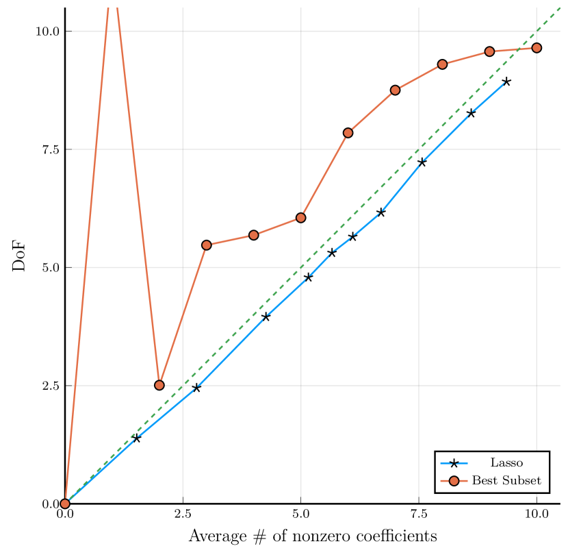
Figure 1: The empirical degrees of freedom of the lasso and the best subset regression on a simulated regression example with $n=20,p=10$.

[21] argued that the search degrees of freedom of the lasso equals the one of the relaxed lasso, which refits with the selected variable set ${\mathcal{A}}$ from the lasso. The argument might not be acceptable since the lasso does not have the refitting step as in the relaxed lasso, so such a search degrees of freedom cannot account for the search effort of the lasso in the adaptive procedure.

3.2.1 Approximate Lasso by Iterative Ridge

We take another perspective to study the degrees of freedom of the lasso by constructing the solution with a linear operator and show that there exists a nonzero modified search degrees of freedom for the lasso.

First of all, let us start with two general scalar functions. Consider $f(u)=|u|$, and

$$g(u,v)=|v|+\frac{1}{2|v|}(u^{2}-v^{2})\,,$$

then we have

$$g(u,u) =f(u)$$ (16)

$$g(u,v) =\frac{u^{2}}{2|v|}+\frac{|v|}{2}\geq 2\sqrt{\frac{u^{2}}{2|v|}\frac{|v|}{2}}=|u|=f(u)\,.$$ (17)

It implies that $g(u,v)$ majorizes $f(u)$, then the minimization of $f(u)$ can be done with the following update

$$u^{(k+1)}=\operatorname*{arg\,min}_{u}g(u,u^{(k)})\,,$$

since $f(u)$ is nonincreasing on the sequence $\{u^{(k)}\}_{k=1}^{\infty}$,

$$\begin{split}f(u^{(k+1)})&=g(u^{(k+1)},u^{(k+1)})\\ &\leq g(u^{k+1},u^{(k)})\\ &\leq g(u^{(k)},u^{(k)})=f(u^{(k)})\,.\end{split}$$

This is well known as the majorize-minimize (MM) algorithm [13].

Note that the objective function in the lasso problem (15) can be written as

$$\mathrm{RSS}(\beta)=\|y-{\mathbf{X}}\beta\|_{2}^{2}+\lambda\|\beta\|_{1}=\|y-{\mathbf{X}}\beta\|_{2}^{2}+\lambda\sum_{i=1}^{p}|\beta_{j}|\,,$$

then one majorization can be chosen to be

$$\mathrm{RSS}(\beta,\theta)=\|y-{\mathbf{X}}\beta\|_{2}^{2}+\lambda\sum_{i=1}^{p}|\theta_{j}|+\lambda\sum_{i=1}^{p}\frac{1}{2|\theta_{j}|}(\beta_{j}^{2}-\theta_{j}^{2})\,.$$

Given current estimation $\beta^{(k)}$, the next update can be written as

$$\hat{\beta}^{(k+1)} =\operatorname*{arg\,min}_{\beta}\mathrm{RSS}(\beta,\hat{\beta}^{(k)})$$

$$=\operatorname*{arg\,min}_{\beta}\|{\mathbf{y}}-{\mathbf{X}}\beta\|_{2}^{2}+\lambda\beta^{\prime}\Psi^{(k)}\beta$$

$$=({\mathbf{X}}^{T}{\mathbf{X}}+\lambda\Psi^{(k)})^{-1}{\mathbf{X}}^{T}{\mathbf{y}}\,,$$

where $\Psi^{(k)}$ is a diagonal matrix with elements $\left\{\frac{1}{2|\beta_{j}^{(k)}|}\right\}_{j=1}^{p}$. The update can be viewed as a generalized ridge regression, and the initialization can be taken to be the ridge estimation,

$$\hat{\beta}^{(1)}=({\mathbf{X}}^{T}{\mathbf{X}}+\lambda{\mathbf{I}})^{-1}{\mathbf{X}}^{T}{\mathbf{y}}\,.$$

Since the lasso tends to do variable selection, some coefficients $\beta_{j}$ would be zero. In the above iteration, although $\beta_{j}$ might not be exactly zero, its inverse would approach infinity, and hence the penalty parameter for the $j$-th coefficient would approach infinity. To overcome such an issue, [23] suggested removing the $j$-th covariate from the model altogether. But based on our experiments, removing the covariates would result in a different solution, which is far from the lasso estimate. Instead, we set the coefficients near zero as a small number, say, $1.0\times 10^{-7}$.

Once the iterative ridge has converged, since the iterative ridge converges to the lasso solution, the lasso solution can be written as

$$\hat{\beta}^{\mathrm{lasso}}=({\mathbf{X}}^{T}{\mathbf{X}}+\lambda\Psi)^{-1}{\mathbf{X}}^{T}{\mathbf{y}}\,,$$

where $\Psi=\operatorname*{diag}\{1/|\hat{\beta}_{1}^{\mathrm{lasso}}|,\ldots,1/|\hat{\beta}_{p}^{\mathrm{lasso}}|\}$, then the fitted value is

$$\hat{\mathbf{y}}={\mathbf{X}}\hat{\beta}^{\mathrm{lasso}}={\mathbf{X}}({\mathbf{X}}^{T}{\mathbf{X}}+\lambda\Psi)^{-1}{\mathbf{X}}^{T}{\mathbf{y}}\triangleq{\mathbf{S}}{\mathbf{y}}\,.$$

It follows that $\operatorname*{tr}({\mathbf{S}})$ might serve as an estimate for the degrees of freedom for the lasso based on Section 2. But Theorem 3, whose proof is given in Appendix C, shows that it is a biased estimate, and it always underestimates.

Theorem 3.

The degrees of freedom for the lasso can be characterized by

$$\mathrm{df}={\mathbb{E}}[\delta+\operatorname*{tr}{\mathbf{S}}({\mathbf{y}})]\,,$$

with

$$\delta=\sum_{i=1}^{n}\sum_{j=1}^{n}\left(\frac{\partial{\mathbf{S}}_{ij}({\mathbf{y}})}{\partial y_{i}}y_{j}\right)\,,$$

where

$$\frac{\partial{\mathbf{S}}({\mathbf{y}})}{\partial y_{i}} =-\lambda{\mathbf{X}}({\mathbf{X}}^{T}{\mathbf{X}}+\lambda\Psi({\mathbf{y}}))^{-1}C_{\hat{\beta}}\cdot$$

$$\qquad\qquad D_{\hat{\beta}}({\mathbf{X}}^{T}{\mathbf{X}}+\lambda\Psi({\mathbf{y}}))^{-1}{\mathbf{X}}^{T}$$

$$C_{\hat{\beta}} =\operatorname*{diag}\left\{\frac{-\operatorname*{sign}(\hat{\beta}_{1})}{2\hat{\beta}_{1}^{2}},\ldots,\frac{-\operatorname*{sign}(\hat{\beta}_{p})}{2\hat{\beta}_{p}^{2}}\right\}$$

$$D_{\hat{\beta}} =\operatorname*{diag}\left\{\frac{\partial\hat{\beta}_{1}}{\partial y_{i}},\ldots,\frac{\partial\hat{\beta}_{p}}{\partial y_{i}}\right\}$$

and $\operatorname*{sign}(x)$ is the sign function, which takes 1 if $x>0$, -1 if $x<0$, and zero if $x=0$, and define $0/0$ as 0 when $\hat{\beta}_{j}=0$.

By the definition of modified search degrees of freedom, we have

$$\mathrm{msdf}=\mathrm{df}-{\mathbb{E}}[\operatorname*{tr}{\mathbf{S}}({\mathbf{y}})]=\delta\,,$$

which can be thought as the amount that comes from the iterations to determine (search) $\Psi$. As a comparison, [21]’s search degrees of freedom can only give the search cost for the relaxed lasso.

In practice, the finite difference can be used to approximate the derivative of $\hat{\beta}$ with respect to ${\mathbf{y}}$, and we can compare the degrees of freedom calculated from Theorems 2 and 3.

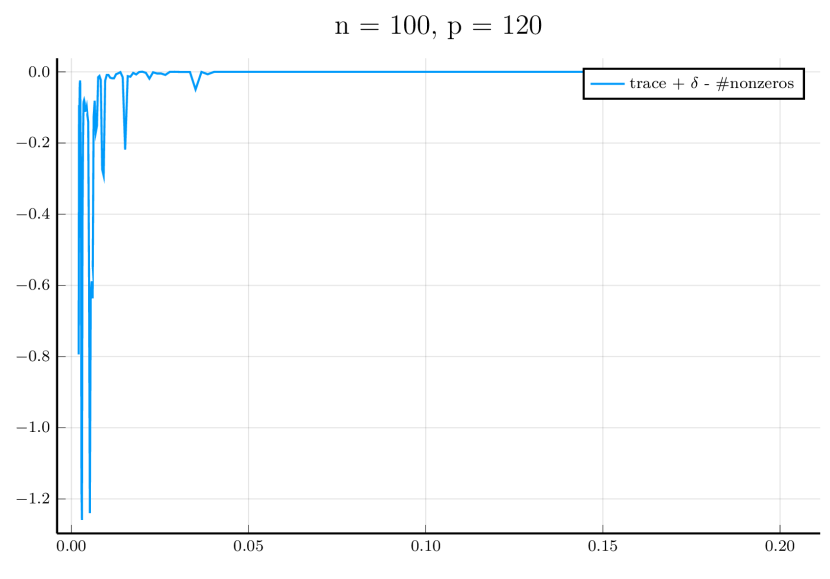
Figure 2: Left panel shows different estimates for the degrees of freedom of the lasso. The dashed line counts the number of nonzero coefficients, and the red curve calculates $\operatorname*{tr}({\mathbf{S}})$, and the green line corrects the red curve by adding $\delta$. Right panel displays the difference between the estimate $\delta+\operatorname*{tr}({\mathbf{S}})$ and the estimate by counting nonzero coefficients.

Figure 2 agrees with Theorem 3, which shows that the trace of the smooth matrix via iterative ridge would always underestimate the degrees of freedom, but these two methods would coincide after adding the corrected term $\delta$.

3.2.2 Examples

Here are some simulations for comparing the solutions, degrees of freedom and GCV for the iterative ridge and the lasso. We generate $\{x_{i1},\ldots,x_{ip},y_{i}\},i=1,\ldots,p$ from

$$y_{i}=\sum_{j=1}^{p}x_{ij}\beta_{j}+\varepsilon_{i}\,,$$

where both $x_{i}$ and $\varepsilon_{i}$ are sampled independently from the standard Gaussian distribution. Let $\beta_{1}=\beta_{2}=\beta_{3}=1$ and $\beta_{4}=\cdots=\beta_{p}=0$ such that the signal-to-noise ratio $\operatorname*{Var}[{\mathbb{E}}(Y\mid X)]/\operatorname*{Var}(\varepsilon)$ is 3.

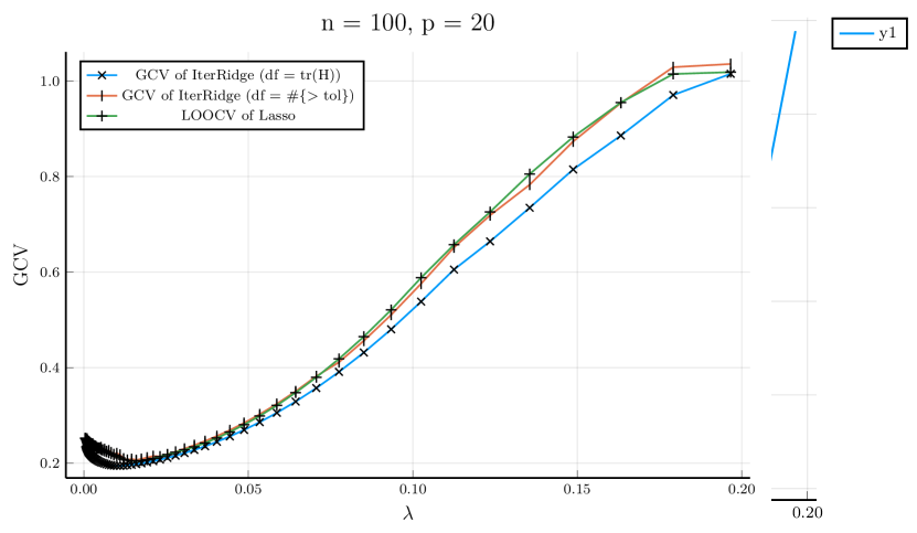
Figure 3: Demo of iterative ridge regression when $n>p$. The left panel shows the ridge solution at each iteration, and a thicker color denotes a solution with more iterations. The middle panel shows the degrees of freedom calculated based on the trace of ${\mathbf{S}}$ at the last iteration, and the ones calculated by counting the number of nonzero coefficients. The right panel shows the GCV calculated based on the iterative ridge and the LOOCV of the lasso.

The left panel of Figure 3 shows that the iterative ridge indeed has a good approximation for the lasso at each $\lambda$. The resulting GCV in the right panel of Figure 3 from iterative ridge can also achieve a good approximation to the leave-one-out cross-validation (LOOCV) of the lasso, regardless of two different degrees of freedom, although the one by counting the number of (nearly) zero coefficients seems better.

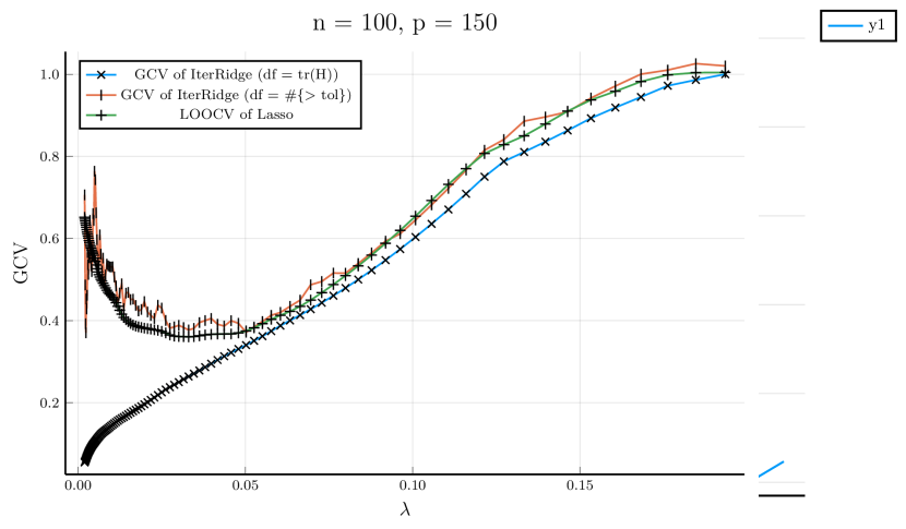
Figure 4: Demo of iterative ridge regression when $n<p$. The left panel shows the ridge solution at each iteration, and a thicker color denotes a solution with more iterations. The middle panel shows the degrees of freedom calculated based on the trace of ${\mathbf{S}}$ at the last iteration, and the ones calculated by counting the number of nonzero coefficients. The right panel shows the GCV calculated based on the iterative ridge and the LOOCV of the lasso.

Figure 4 shows the results when $n<p$. The iterative ridge again converges to the lasso solution, and the GCV curve via the degrees of freedom by counting the (nearly) zero coefficients is close to LOOCV, but the GCV curve via the trace of ${\mathbf{S}}$ has different behavior. The reason is that the trace underestimates the degrees of freedom when $\lambda$ is small.

4 Tree-based and Tree-like Methods

4.1 Regression Tree

The phenomenon that the degrees of freedom can be larger than the number of free parameters has also been observed in the regression tree. The data consists of $p$ inputs and a response: $\{(x_{i},y_{i})\}_{i=1}^{n}$ with $x_{i}=(x_{i1},\ldots,x_{ip})$. To grow a regression tree, suppose there is a partition into $M$ regions $R_{1},\ldots,R_{M}$, and we model the response as a constant $c_{m}$ in each region. The conventional criterion for the regression tree is the minimization of the sum of squares $\sum(y_{i}-f(x_{i}))^{2}$. It can be shown that the best $\hat{c}_{m}$ is just the average of $y_{i}$ in the region $R_{m}$, then the fitting function can be written as

$$\hat{\mu}(x) =\sum_{m=1}^{M}\hat{c}_{m}I(x\in R_{m})$$

$$=\sum_{m=1}^{M}\frac{\sum_{j=1}^{n}y_{j}I(x_{j}\in R_{m})}{\sum_{k=1}^{n}I(x_{k}\in R_{m})}I(x\in R_{m})\,.$$

Switch the summation for $m$ and $j$ in the numerator, then for each $x_{i}$, the fitting can be rewritten as

$$\hat{y}_{i}=\hat{\mu}(x_{i}) =\sum_{j=1}^{n}\frac{\sum_{m=1}^{M}y_{j}I(x_{j}\in R_{m})}{\sum_{k=1}^{n}I(x_{k}\in R_{m})}I(x_{i}\in R_{m})$$

$$=\sum_{j=1}^{n}\frac{\sum_{m=1}^{M}I(x_{j}\in R_{m})I(x_{i}\in R_{m})}{\sum_{k=1}^{n}I(x_{j}\in R_{m})}y_{j}$$

$$\triangleq\sum_{j=1}^{n}{\mathbf{S}}_{ij}y_{j}\,,$$

which yields

$$\hat{\mathbf{y}}={\mathbf{S}}{\mathbf{y}}\,.$$

We have

$$\operatorname*{tr}({\mathbf{S}})=\sum_{i=1}^{n}{\mathbf{S}}_{ii} =\sum_{i=1}^{n}\sum_{m=1}^{M}\frac{I(x_{i}\in R_{m})}{\sum_{k=1}^{n}I(x_{k}\in R_{m})}$$

$$=\sum_{m=1}^{M}\frac{\sum_{i=1}^{n}I(x_{i}\in R_{m})}{\sum_{k=1}^{n}I(x_{k}\in R_{m})}=M\,.$$

It follows that the modified search degrees of freedom is

$$\mathrm{msdf}=\mathrm{df}-M\,.$$

On the other hand, the search degrees of freedom might not be proper for the regression trees since the active variable set ${\mathcal{A}}$ is not clear to define. And even we can identify the active set, it always relates the search degrees of freedom to the full least squares on the active set instead of the regression tree itself.

The partition can be found by a greedy binary partition algorithm, followed by an optional pruning procedure [1].

For simplicity, we skip the pruning procedure. The resulting tree would be complete, then the depth and the number of terminal nodes $M$ satisfy $M=2^{\text{depth}}$. Table 3 shows the empirical degrees of freedom under different depths for simulated examples $p=1,5$ and $10$. Except for $M=1$, all $\hat{\mathrm{df}}$’s are much larger than the corresponding number of coefficients $M$. Similarly, we account for the surplus as the cost for searching the partition variable and the associated cutpoint.

Table 3: Empirical degrees of freedom of regression trees on simulated examples $p=1,5,10$ and $n=100$. The results are averaged over 10 simulations, with the standard error in parentheses.

depth	$M$	$\hat{\mathrm{df}}$
		$p=1$	$p=5$	$p=10$
0	1	1.01 (0.05)	1.02 (0.04)	1.00 (0.05)
1	2	5.71 (0.08)	8.71 (0.07)	9.87 (0.10)
2	4	11.84 (0.20)	18.38 (0.17)	21.62 (0.22)
3	8	19.80 (0.18)	30.14 (0.27)	35.01 (0.35)
4	16	28.97 (0.29)	42.06 (0.44)	48.49 (0.35)

[25] also did similar experiments which revealed a similar phenomenon for the regression tree.

4.2 Multiple Adaptive Regression Splines

Multiple Adaptive Regression Splines (MARS) is an adaptive procedure for regression proposed by [4]. It is closely related to the tree-based method since it can be viewed as a generalization of stepwise linear regression of the tree regression method to improve the latter’s performance [11]. Specifically, with some minor changes, the MARS forward procedure would be the same as the tree-growing algorithm.

The model takes the form of an expansion in piecewise linear basis functions of the form $(x-t)_{+}$ and $(t-x)_{+}$. For each input $X_{j}$ and each observed value $x_{ij}$ of that input, construct the collection of basis functions,

$${\cal{D}}=\left\{(X_{j}-t)_{+},(t-X_{j})+\right\},\;t\in\{x_{ij}\}_{i=1}^{n},j=1,\ldots,p\,.$$

The model has the form

$$\mu(X)=\beta_{0}+\sum_{m=1}^{M}\beta_{m}h_{m}(X)\,,$$

where each $h_{m}(X)$ is a function in the collection $\cal{D}$, or a product of two or more such functions. If all $h_{m}(X)$ are restricted in $\cal D$, we would call it an additive model (degree = 1), otherwise, we call it an interaction model (degree > 1) when there exist products of basis functions in $\cal{D}$.

MARS consists of a forward step and a backward step. The forward step adds the basis functions from the collection $\mathcal{D}$ into the model, either to be a new basis function or to multiply the existing function in the model. Similar to the pruning procedure in the tree-based methods, MARS also applies a backward deletion, and it uses the generalized cross-validation as the stop criterion,

$$\mathrm{GCV}(M)=\frac{\sum_{i=1}^{n}(y_{i}-\hat{\mu}_{M}(x_{i}))^{2}}{(1-\tilde{C}(M)/N)^{2}}\,,$$

where $\tilde{C}(M)$ is the effective number of parameters in the model, i.e., the degrees of freedom. It accounts both for the number of terms in the models, plus the number of parameters used in selecting the optimal positions of the knots. It is pre-determined before the model selection, so we call the nominal degrees of freedom.

4.2.1 Search Cost and Nominal Degrees of Freedom

[4] proposed

$$\tilde{C}(M)=C(M)+c\cdot M\,,$$

where $M$ is the number of nonconstant basis functions, $C(M)$ is the number of linearly independent basis functions, and the quantity $c$ represents the optimization cost for each basis function. He suggested that $c$ takes 2 for the additive model due to the expected decrease in the average-squared residual by adding a single knot to make a piecewise-linear model. If all basis functions (including the constant functions) are linearly independent, then we have

$$\tilde{C}(M)=(M+1)+c\cdot M=(1+c)\cdot M+1\,,$$

which coincides with the degrees of freedom formula in [5] when $c$ is chosen to be 2. [4] also discussed the best value of $c$ in general cases. He mentioned that the best value for $c$ would depend on the number of basis functions, the number of samples, and the distribution of the covariates. Based on simulation studies, he suggested $c\in[2,4]$, and recommended a "fairly effective, if somewhat crude" choice $c=3$. The discussion paper [17] related the choice $c=3$ to the Chi-squared distribution with approximated 3 degrees of freedom under the null hypothesis for testing if $\beta=0$ in the following two-phase regression,

$$Y_{i}=b_{0}+b_{1}t_{i}+\beta(t_{i}-\theta)_{+}+\epsilon_{i}\,.$$

However, [11] adopted a slightly different formula. To align the notations, let $r\triangleq C(M)$ be the number of linearly independent basis functions, and $K$ be the number of knots used in the forward procedure, then they wrote that

$$\tilde{C}(M)=r+c\cdot K\,,$$

where $c$ again takes 2 for additive models and 3 for interaction models. In other words, [11] suggested $c$ cost for each knot instead of each basis function in [4]. Note that each knot $t$ has two basis functions $(x-t)_{+}$ and $(t-x)_{+}$. In practice, [10]’s R package mda and [16]’s R package earth determine the number of knots as $K=\frac{r-1}{2}$, and hence

$$\tilde{C}(M)=r+c\cdot\frac{r-1}{2}\,,$$ (18)

After minimizing GCV, we can determine the optimal $M^{\star}$ and evaluate the actual degrees of freedom $\hat{\mathrm{df}}$.

4.2.2 Correction for Self-consistency

For MARS, the self-consistency does not hold since there is usually a gap between the actual degrees of freedom $\hat{\mathrm{df}}$ approximated by Algorithm 1 and the nominal degrees of freedom $\tilde{C}(M)$, as shown in Figure 5. Each point in Figure 5 represents a MARS fitting with $\tilde{C}(M)$ as $y$-coordinate and $\hat{\mathrm{df}}$ as $x$-coordinate. We vary the maximum number of knots (parameter nk in the function earth::earth from R package earth) in the forward procedure from 1 to 100, and for each nk, perform a MARS fitting, then connect the points along the parameter nk. If the self-consistency property holds, the points will lie on the dashed line $y=x$. The default setting denoted by triangle symbols refers to $c=2$ for additive models (degree = 1) and 3 for interaction models (degree > 1), which is exactly the default setting in R package earth. The default setting is always away from the dashed line in all scenarios. With small $p=1$, $\tilde{C}(M)$ is larger than the empirical degrees of freedom $\hat{\mathrm{df}}$. In contrast, $\tilde{C}(M)$ is smaller than $\hat{\mathrm{df}}$ when larger $p=50$. For a moderate $p=10$, although it coincides with the dashed line in the middle region, $\tilde{C}(M)$ is even smaller when $\hat{\mathrm{df}}$ is smaller, while $\tilde{C}(M)$ is even larger when $\hat{\mathrm{df}}$ is larger. Both the additive model (degree = 1) and the interaction model (degree > 1) exhibit the same undesired behavior.

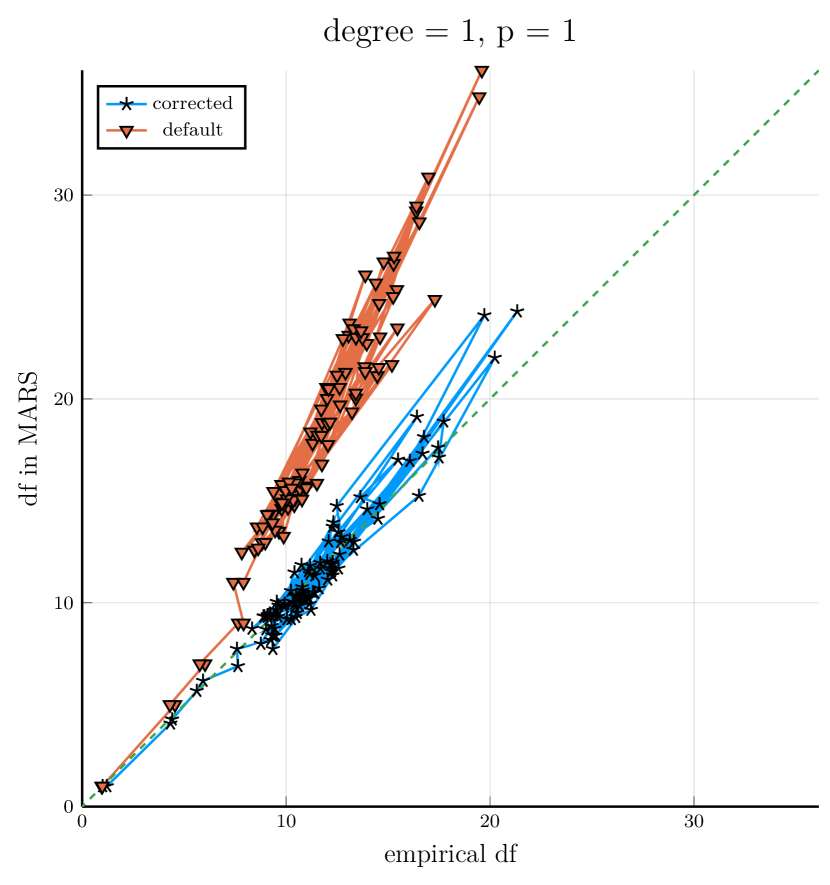
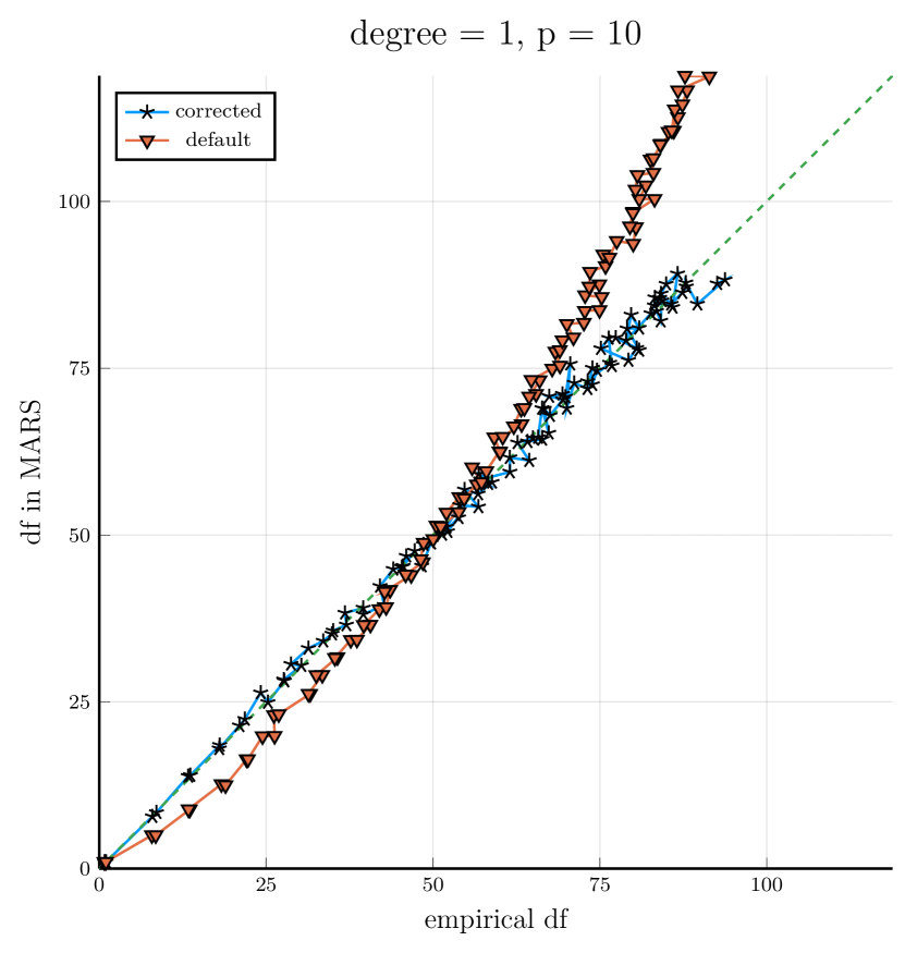
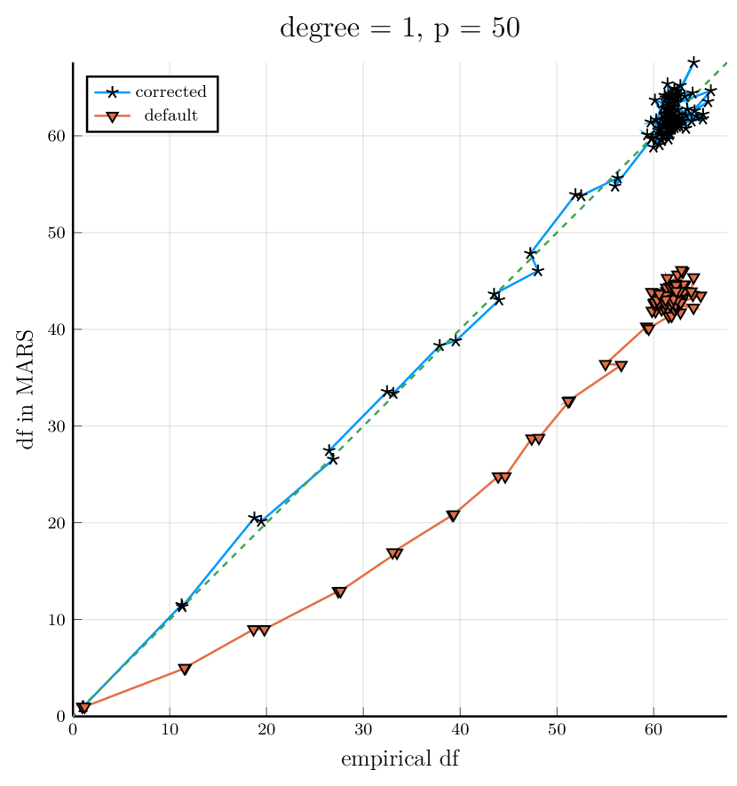
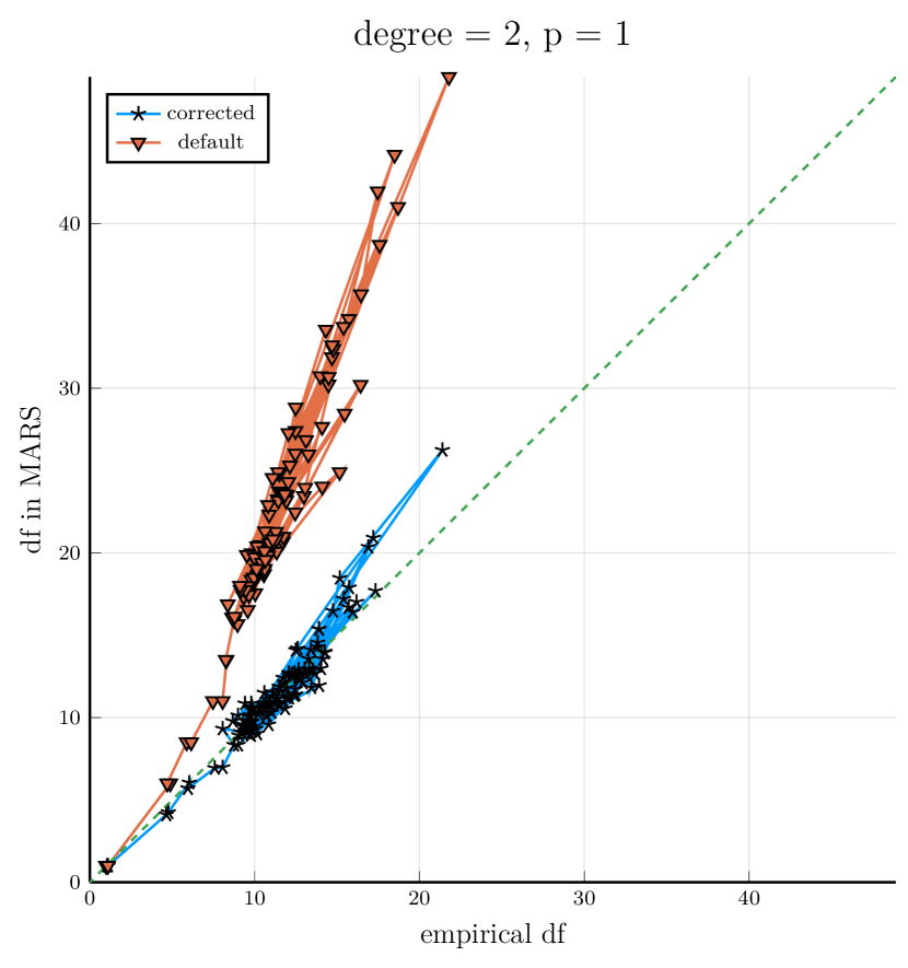
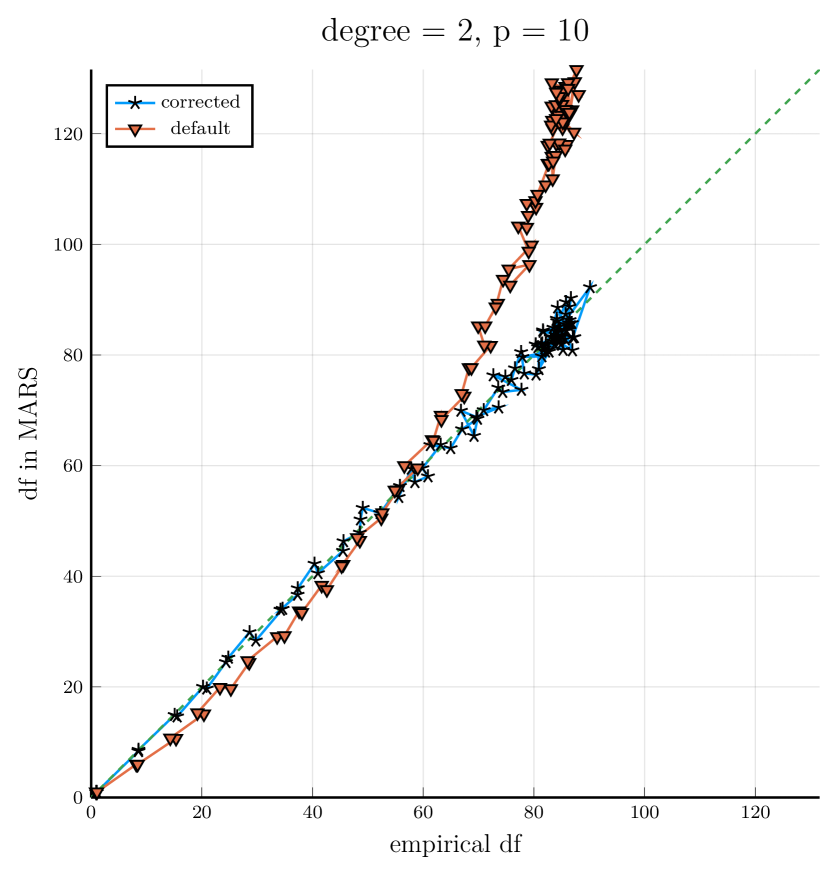
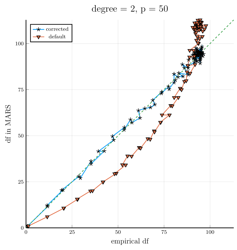
Figure 5: Empirical degrees of freedom $\hat{\mathrm{df}}$ and MARS’ degrees of freedom $\tilde{C}(M)$ with the default penalty factor and the corrected penalty factor in various scenarios indexed by the degree and the number of predictors $p$.

To fulfill the self-consistency property, we allow $c$ to be a tuning parameter instead of the fixed values, 2 (for additive models) or 3 (for interaction models). We propose an iterative procedure, summarized in Algorithm 2, to estimate the penalty factor $c$. Figure 5 shows that the degrees of freedom corrected by Algorithm 2 lies on the dashed line, which indicates that the self-consistency property has been achieved using our algorithm. We also wrap up the algorithm in an R package earth.dof.patch for people who use MARS with its R package earth.

Algorithm 2 Correct Degrees of Freedom in MARS

1:  while not converged do

2:     Calculate the empirical degrees of freedom $\hat{\mathrm{df}}$ for MARS with penalty factor $c$ by Algorithm 1.

3:     Extract the nominal degrees of freedom $\tilde{C}(M)$ of MARS, and calculate $r=\frac{\tilde{C}(M)+c/2}{c/2+1}$ from Equation (18).

4:     if $r=1$ then

5:        break

6:     else

7:        Update penalty factor by equaling the empirical $\hat{\mathrm{df}}$ to MARS’s nominal degrees of freedom $\tilde{C}(M)$,

$$c=\frac{2(\hat{\mathrm{df}}-r)_{+}}{r-1}\,.$$

8:     end if

9:  end while

10:  return  Penalty factor $c$.

To check whether the corrected degrees of freedom can improve the performance, we consider the tensor-product example in Section 9.4.2 of [11],

$$Y=(X_{1}-1)_{+}+(X_{1}-1)_{+}\cdot(X_{2}-0.8)_{+}+0.12\varepsilon\,,$$ (19)

where the predictors $X_{1},\ldots,X_{p}$ and errors $\varepsilon$ follow independent standard Gaussian distributions. Let $\mu(x)$ be the true mean of $Y$, and let

$$\mathrm{MSE}_{0}=\mathrm{ave}_{x\in\mathrm{Test}}(\bar{y}-\mu(x))^{2}\,,$$ (20)

$$\mathrm{MSE}=\mathrm{ave}_{x\in\mathrm{Test}}(\hat{\mu}(x)-\mu(x))^{2}\,,$$ (21)

which represent the mean-square error of the constant model and the fitted MARS model, respectively. The proportional decrease in model error is

$$R^{2}=\frac{\mathrm{MSE}_{0}-\mathrm{MSE}}{\mathrm{MSE}_{0}}\,.$$

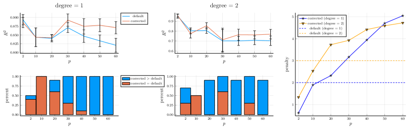
Figure 6: Proportional decrease in model error $R^{2}$ when MARS with the default and corrected degrees of freedom are applied in different scenarios indexed by the number of predictors $p$. The right panel shows the corrected penalty factor. In the left panel consisting of 2-by-2 grid subplots, the top two display the average $R^{2}$ among 10 replications with the standard errors as the error bars along the number of predictors $p$. The bottom two bar plots display the percent of the corrected method is better than (or equal to) the default method.

Although the true model in Equation (19) is generated with an interaction term, we consider the fitting with an additive model (degree = 1) in addition to fitting it with an interaction model (degree = 2). Figure 6 shows the proportional decrease in model error $R^{2}$ when MARS with the default and corrected degrees of freedom are applied in different scenarios indexed by the number of predictors $p$. In both additive models and interaction models scenarios, the corrected MARS can improve the MSE, especially when the number of predictors $p$ is large. The bar plots show that the corrected approach always outperforms the default method when $p$ is large. On the other hand, the results are quite close when $p$ is small. The right panel shows the corrected penalty factor. When $p$ is small, the corrected penalty factor is smaller than the default penalty factor, and when $p$ is large, the corrected penalty factor is larger than the default one. The phenomenon is consistent with Figure 5, where the nominal degrees of freedom tend to be larger than the actual degrees of freedom when $p=1$ and on the other hand, it is smaller than the actual degrees of freedom when $p$ is large.

5 Discussions

Through a number of model fitting procedures, we have shown that the degrees of freedom usually does not equal the number of free parameters. For adaptive approaches such as regression trees and best subset regressions, the degrees of freedom is larger than the number of the free parameters, and the excess amount is referred to as the search degrees of freedom; for regularized methods such as ridge regressions and splines, the degrees of freedom would be smaller than the number of free parameters. We extend the definition and propose the modified search degrees of freedom, which can account for the search cost of a linear operator. Remarkably, the degrees of freedom of the lasso is exactly the number of selected coefficients, but we take another perspective and find that the lasso also exhibits a nonzero search cost. The modified search degrees of freedom also works for procedures with augmented spaces, such as splines methods, tree-based methods, and MARS.

We also investigate the gap between the nominal degrees of freedom and the actual degrees of freedom when the degrees of freedom is served as a parameter in model selection. We define the self-consistency property when there is no gap between these two degrees of freedom. For MARS, which violates the self-consistency property, we propose a correction procedure to fulfill the self-consistency property. It turns out that the corrected approach can significantly improve the fitting performance.

Despite our efforts to improve the understanding of the degrees of freedom by developing the search cost and self-consistency concepts, here are some limitations that need future development.

• The general definition in Equation (6) assumes homogeneous variance, but practically there are many heterogeneous cases. There is a need to discuss the generalization to heterogeneous situations.

• The phenomenon that the degrees of freedom might be larger than the number of coefficients can be easily observed in simulations, but there is little theoretical support and discussion in the literature. It would be more helpful to derive some closed form for the degrees of freedom, at least in some special cases, such as the best subset regression (Section 3.1) in the orthogonal setting in Theorem 1.

• The degrees of freedom can be viewed as the expectation of divergence $D({\mathbf{y}})$, as shown in Equation (7). For linear smoothers, the divergence is a constant, independent of ${\mathbf{y}}$, and hence equal to the degrees of freedom. However, there are other situations in which only the divergence is accessible, such as the monotone splines in Section 2.2. In that case, treating the divergence as an estimate for the degrees of freedom might be problematic when the variance of divergence is large. It might be necessary to investigate the uncertainty of divergence $\operatorname*{Var}[D({\mathbf{y}})]$.

• As suggested from the definition in Equation (6), the degrees of freedom focuses on the in-sample prediction $\hat{\mu}_{i}$ instead of out-of-sample prediction. [14] extended the definition to out-of-sample prediction, and termed as predictive degrees of freedom. The authors claimed that it could help explain the “double descent” phenomenon in over-parametrized interpolating models (e.g., [26] and [7]). Currently, their predictive degrees of freedom is only discussed for linear regressions. It would be interesting to check more connections with other models, such as MARS in Section 4.2.

Appendix A Proof of Proposition 1

First of all, we state Stein’s Lemma.

Lemma 1 ([19]).

Let $X\sim N(\xi,\sigma^{2}{\mathbf{I}})$ be a $p$-dimensional random vector. If $h:\mathrm{I\!R}^{p}\rightarrow\mathrm{I\!R}$ is an almost differentiable function with ${\mathbb{E}}\|\nabla h(X)\|_{2}<\infty$, then

$${\mathbb{E}}[\nabla h(X)]=\frac{1}{\sigma^{2}}{\mathbb{E}}[(X-\xi)h(X)]\,.$$

Apply Lemma 1 on ${\mathbf{y}}\sim N(\mu,\sigma^{2}{\mathbf{I}})$,

$$\frac{1}{\sigma^{2}}{\mathbb{E}}[({\mathbf{y}}-\mu)\hat{\mu}_{i}({\mathbf{y}})]={\mathbb{E}}[\nabla\hat{\mu}_{i}({\mathbf{y}})]\,,$$

in which the $i$-th component is

$$\frac{1}{\sigma^{2}}{\mathbb{E}}[(y_{i}-\mu_{i})\hat{\mu}_{i}({\mathbf{y}})]={\mathbb{E}}[\nabla_{i}\hat{\mu}_{i}({\mathbf{y}})]={\mathbb{E}}\left[\frac{\partial\hat{\mu}_{i}}{\partial y_{i}}({\mathbf{y}})\right]\,,$$

and $\hat{\mu}_{i}$ is assumed to be almost differentiable with ${\mathbb{E}}\|\nabla\hat{\mu}_{i}\|_{2}<\infty$, then

$$\begin{split}\mathrm{df}(\hat{\mu})&=\frac{1}{\sigma^{2}}\sum_{i=1}^{n}\operatorname*{Cov}(y_{i},\hat{\mu}_{i})\\ &=\frac{1}{\sigma^{2}}\sum_{i=1}^{n}{\mathbb{E}}[(y_{i}-\mu_{i})\hat{\mu}_{i}({\mathbf{y}})]\\ &={\mathbb{E}}\left[\sum_{i=1}^{n}\frac{\partial\hat{\mu}_{i}}{\partial y_{i}}({\mathbf{y}})\right]\triangleq{\mathbb{E}}[D({\mathbf{y}})]\,,\end{split}$$ (22)

where $D({\mathbf{y}})$ is called the divergence of $\hat{\mu}$, and Equation (7) is referred to as Stein’s formula for degrees of freedom [21].

This degrees of freedom has been used in SURE, which starts by expanding

$$R ={\mathbb{E}}\|\mu-\hat{\mu}\|^{2}={\mathbb{E}}\|\mu-{\mathbf{y}}+{\mathbf{y}}-\hat{\mu}\|^{2}$$

$$={\mathbb{E}}\|\mu-{\mathbf{y}}\|^{2}+{\mathbb{E}}\|{\mathbf{y}}-\hat{\mu}\|^{2}+2{\mathbb{E}}(\mu-{\mathbf{y}})^{T}({\mathbf{y}}-\hat{\mu})\,,$$

where

$${\mathbb{E}}(\mu-{\mathbf{y}})^{T}({\mathbf{y}}-\hat{\mu})$$

$$={\mathbb{E}}({\mathbf{y}}-\mu)^{T}(\hat{\mu}-{\mathbf{y}})$$

$$={\mathbb{E}}({\mathbf{y}}-\mu)^{T}(\hat{\mu}-{\mathbb{E}}\hat{\mu}+{\mathbb{E}}\hat{\mu})-{\mathbb{E}}({\mathbf{y}}-\mu)^{T}({\mathbf{y}}-\mu+\mu)$$

$$={\mathbb{E}}({\mathbf{y}}-\mu)^{T}(\hat{\mu}-{\mathbb{E}}\hat{\mu})-{\mathbb{E}}({\mathbf{y}}-\mu)^{T}({\mathbf{y}}-\mu)$$

$$=\sum_{i=1}^{n}\operatorname*{Cov}(y_{i},\hat{\mu}_{i})-{\mathbb{E}}\|{\mathbf{y}}-\mu\|^{2}\,,$$

then

$$R =-{\mathbb{E}}\|{\mathbf{y}}-\mu\|^{2}+{\mathbb{E}}\|{\mathbf{y}}-\hat{\mu}\|^{2}+2\sum_{i=1}^{n}\operatorname*{Cov}(y_{i},\hat{\mu}_{i})$$

$$=-n\sigma^{2}+{\mathbb{E}}\|{\mathbf{y}}-\hat{\mu}\|^{2}+2\sigma^{2}\mathrm{df}(\hat{\mu})\,.$$

If $\hat{\mu}$ is almost differentiable as a function of ${\mathbf{y}}$, then

$$\hat{R}=-n\sigma^{2}+\|{\mathbf{y}}-\hat{\mu}\|^{2}+2\sigma^{2}\sum_{i=1}^{n}\frac{\partial\hat{\mu}_{i}}{\partial y_{i}}$$

is an unbiased estimate for $R$, i.e., ${\mathbb{E}}(\hat{R})=R$, and the estimate $\hat{R}$ is called Stein’s unbiased risk estimate (SURE).

Appendix B Proof of Proposition 3

[2] studied the degrees of freedom of nonparametric estimators that are obtained as minimizers of the least squares criterion with linear constraints and/or quadratic penalties,

$$\begin{split}(\hat{\theta}({\mathbf{y}}),\hat{\xi}({\mathbf{y}}))\in&\operatorname*{arg\,min}_{\theta,\xi}\frac{1}{2}\|\theta-{\mathbf{y}}\|_{2}^{2}+d^{T}\xi+\frac{\lambda}{2}\|\xi\|_{2}^{2}\\ \mathrm{s.t.}\;&A\xi+B\theta\leq c\,,\end{split}$$ (23)

where the belong symbol $\in$ indicates that the solution might not be unique, $A=[a_{1},\ldots,a_{m}]^{T}\in\mathrm{I\!R}^{m\times p},B=[b_{1},\ldots,b_{m}]^{T}\in\mathrm{I\!R}^{m\times n},c\in\mathrm{I\!R}^{m},d\in\mathrm{I\!R}^{p}$ and $\lambda\geq 0$ is a regularization parameter. They proved the following theorem.

Theorem 4 ([2]).

Suppose that $-d=A^{T}u$ for some $u\geq 0$ whenever $\lambda=0$. For any ${\mathbf{y}}\in\mathrm{I\!R}^{n}$, let $(\hat{\theta}({\mathbf{y}}),\hat{\xi}({\mathbf{y}}))$ be any solution for Equation (23) and let

$$J_{\mathbf{y}}:=\{1\leq i\leq m:\langle a_{i},\hat{\xi}({\mathbf{y}})\rangle+\langle b_{i},\hat{\theta}({\mathbf{y}})\rangle=c_{i}\}$$

and $A_{J_{\mathbf{y}}}$ and $B_{J_{\mathbf{y}}}$ be the submatrices of $A$ and $B$ with rows in the set $J_{\mathbf{y}}$. Let $I_{\mathbf{y}}\subseteq J_{\mathbf{y}}$ be the index set of maximal independent rows of the matrix $[A_{J_{\mathbf{y}}},B_{J_{\mathbf{y}}}]$, that is, the set of vectors $\{[a_{i}^{T},b_{i}^{T}],i\in I_{\mathbf{y}}\}$ are linearly independent.

If $d=0,\lambda=0$, then for almost everywhere ${\mathbf{y}}$, the divergence $D({\mathbf{y}})=n-|I_{\mathbf{y}}|+\operatorname*{rank}(A_{I_{\mathbf{y}}})$ and $\mathrm{df}(\hat{\theta}({\mathbf{y}}))={\mathbb{E}}[D({\mathbf{y}})]$ (note that the index set $I_{\mathbf{y}}$ is random).

For the degrees of freedom of $\hat{\mu}^{\mathrm{mono},\mathrm{cubic}}(J)$, we give the proof as follows.

Proof.

Let $\xi=\gamma$ and $\theta={\mathbf{B}}\gamma$, then

$$\arg\min_{\beta}\|{\mathbf{y}}-{\mathbf{B}}\gamma\|^{2}_{2}\quad\text{s.t.}\quad K\gamma\leq 0\,,$$

where $K$ is a $(J-1)\times J$ matrix,

$$K_{ij}=\begin{cases}1&i=j=1,\ldots,J-1\\ -1&j=i+1=2,\ldots,J\\ 0&\text{otherwise}\end{cases}$$

The object function can be rewritten as

$$\arg\min_{\theta}\|{\mathbf{y}}-\theta\|^{2}_{2}$$

$${\mathbf{B}}\xi-{\mathbf{I}}_{n}\theta\leq 0$$

$$-{\mathbf{B}}\xi+{\mathbf{I}}_{n}\theta\leq 0$$

$$K\xi+\boldsymbol{0}_{n}\theta\leq 0$$

and let

$$A=\begin{bmatrix}{\mathbf{B}}_{n\times J}\\ -{\mathbf{B}}_{n\times J}\\ K_{(J-1)\times J}\end{bmatrix}\qquad B=\begin{bmatrix}-{\mathbf{I}}_{n}\\ {\mathbf{I}}_{n}\\ \boldsymbol{0}_{(J-1)\times n}\end{bmatrix}$$

Note that the first $2n$ rows would always be in the index set $J_{\mathbf{y}}$, and $I_{\mathbf{y}}$ would take $n$ linearly independent rows from them. If there are $m_{\mathbf{y}}$ (depends on ${\mathbf{y}}$) equal adjacent pairs of $\gamma$, and these corresponding row vectors are also linearly independent with the first $2n$ rows, then

$$|I_{\mathbf{y}}|=n+m_{\mathbf{y}}$$

If $n>p$, then we always have $\operatorname*{rank}(A_{I_{\mathbf{y}}})=p$. Thus, the divergence is

$$D({\mathbf{y}})=n-(n+m_{\mathbf{y}})+p=p-m_{\mathbf{y}}\triangleq U_{\mathbf{y}}\,,$$

where $U_{y}$ is the number of unique coefficients, then

$$\mathrm{df}={\mathbb{E}}[D({\mathbf{y}})]=p-{\mathbb{E}}[m_{\mathbf{y}}]={\mathbb{E}}[U_{\mathbf{y}}]\,,$$

where the randomness comes from the index set $I_{\mathbf{y}}$. ∎

Appendix C Proof of Theorem 3

Proof.

Note that ${\mathbf{S}}$ depends on $y$ via $\Psi$. By the definition of degrees of freedom and consider the form derived from Stein’s lemma.

The degrees of freedom is

$$\mathrm{df}=\frac{1}{\sigma^{2}}\sum_{i=1}^{n}\operatorname*{Cov}(\hat{y}_{i},y_{i})={\mathbb{E}}\sum_{i=1}^{n}\left[\frac{\partial\hat{y}_{i}}{\partial y_{i}}\right]\,,$$

where

$$\hat{y}_{i}=\sum_{j=1}^{n}{\mathbf{S}}_{ij}({\mathbf{y}})y_{j}\,.$$

It follows that

$$\frac{\partial\hat{y}_{i}}{\partial y_{i}} =\sum_{j=1}^{n}\left(\frac{\partial{\mathbf{S}}_{ij}({\mathbf{y}})}{\partial y_{i}}y_{j}+{\mathbf{S}}_{ij}({\mathbf{y}})\frac{\partial y_{j}}{\partial y_{i}}\right)$$

$$=\sum_{j=1}^{n}\left(\frac{\partial{\mathbf{S}}_{ij}({\mathbf{y}})}{\partial y_{i}}y_{j}\right)+{\mathbf{S}}_{ii}({\mathbf{y}})$$

Now calculate the derivative

$$\frac{\partial{\mathbf{S}}({\mathbf{y}})}{\partial y_{i}}\,,$$

where

$${\mathbf{S}}({\mathbf{y}})={\mathbf{X}}({\mathbf{X}}^{\prime}{\mathbf{X}}+\lambda\Psi({\mathbf{y}}))^{-1}{\mathbf{X}}^{T}\,.$$

The $j$-th diagonal element

$$\Psi_{jj}({\mathbf{y}})=\frac{1}{2|\hat{\beta}_{i}({\mathbf{y}})|}$$

where $\hat{\beta}({\mathbf{y}})$ is the converged iterative ridge solution, i.e., the lasso solution. Note that

$$\frac{\partial\Psi_{jk}({\mathbf{y}})}{\partial y_{i}}=\begin{cases}0&j\neq k\\ \frac{\partial\Psi_{jj}({\mathbf{y}})}{\partial y_{i}}&j=k\end{cases}$$

that is,

$$\frac{\partial\Psi({\mathbf{y}})}{\partial y_{i}}=\operatorname*{diag}\left\{\frac{\partial\Psi_{11}({\mathbf{y}})}{\partial y_{i}},\ldots,\frac{\partial\Psi_{pp}({\mathbf{y}})}{\partial y_{i}}\right\}\,.$$

and by chain rule,

$$\frac{\partial\Psi_{jj}({\mathbf{y}})}{\partial y_{i}}=\frac{-\operatorname*{sgn}(\hat{\beta}_{j})}{2\hat{\beta}_{j}^{2}}\frac{\partial\hat{\beta}_{j}}{\partial y_{i}}\,.$$

Let

$$C_{\hat{\beta}} =\operatorname*{diag}\left\{\frac{-\operatorname*{sgn}(\hat{\beta}_{1})}{2\hat{\beta}_{1}^{2}},\ldots,\frac{-\operatorname*{sgn}(\hat{\beta}_{p})}{2\hat{\beta}_{p}^{2}}\right\}$$

$$D_{\hat{\beta}} =\operatorname*{diag}\left\{\frac{\partial\hat{\beta}_{1}}{\partial y_{i}},\ldots,\frac{\partial\hat{\beta}_{p}}{\partial y_{i}}\right\}$$

where $\operatorname*{sgn}(x)$ is the sign function, which takes zero if $x=0$, and define $0/0$ as 0 when $\hat{\beta}_{j}=0$ since it is not differentiable at zero for $\psi(t)=1/2|t|$. By chain rule, we have

$$\frac{\partial{\mathbf{S}}({\mathbf{y}})}{\partial y_{i}} =-\lambda{\mathbf{X}}({\mathbf{X}}^{\prime}{\mathbf{X}}+\lambda\Psi({\mathbf{y}}))^{-1}C_{\hat{\beta}}\cdot$$

$$\qquad\qquad D_{\hat{\beta}}({\mathbf{X}}^{\prime}{\mathbf{X}}+\lambda\Psi({\mathbf{y}}))^{-1}{\mathbf{X}}^{T}$$

∎

References

• [1] Leo Breiman, Jerome H. Friedman, Richard A. Olshen and Charles J. Stone “Classification and Regression Trees” New York: Wadsworth, 1994
• [2] Xi Chen, Qihang Lin and Bodhisattva Sen “On Degrees of Freedom of Projection Estimators with Applications to Multivariate Nonparametric Regression” In Journal of the American Statistical Association 115.529, 2020, pp. 173–186 DOI: 10.1080/01621459.2018.1537917
• [3] Bradley Efron “How Biased Is the Apparent Error Rate of a Prediction Rule?” In Journal of the American Statistical Association 81.394 [American Statistical Association, Taylor & Francis, Ltd.], 1986, pp. 461–470 DOI: 10.2307/2289236
• [4] Jerome H. Friedman “Multivariate Adaptive Regression Splines” In The Annals of Statistics 19.1 Institute of Mathematical Statistics, 1991, pp. 1–67 JSTOR: https://www.jstor.org/stable/2241837
• [5] Jerome H. Friedman and Bernard W. Silverman “Flexible Parsimonious Smoothing and Additive Modeling” In Technometrics 31.1 [Taylor & Francis, Ltd., American Statistical Association, American Society for Quality], 1989, pp. 3–21 DOI: 10.2307/1270359
• [6] I.. Good “What Are Degrees of Freedom?” In The American Statistician 27.5, 1973, pp. 227–228 DOI: 10.1080/00031305.1973.10479042
• [7] Trevor Hastie, Andrea Montanari, Saharon Rosset and Ryan J. Tibshirani “Surprises in High-Dimensional Ridgeless Least Squares Interpolation” In The Annals of Statistics 50.2 Institute of Mathematical Statistics, 2022, pp. 949–986 DOI: 10.1214/21-AOS2133
• [8] Trevor Hastie and Werner Stuetzle “Principal Curves” In Journal of the American Statistical Association 2.4, 1989, pp. 183–190
• [9] Trevor Hastie and Robert Tibshirani “Generalized Additive Models” London: Chapman & Hall, 1990
• [10] Trevor Hastie and Robert Tibshirani “mda: Mixture and Flexible Discriminant Analysis (Version 0.5-3)”, 2022 URL: https://CRAN.R-project.org/package=mda
• [11] Trevor Hastie, Robert Tibshirani and Jerome Friedman “The Elements of Statistical Learning: Data Mining, Inference, and Prediction” Springer Science & Business Media, 2009
• [12] James S. Hodges and Daniel J. Sargent “Counting Degrees of Freedom in Hierarchical and Other Richly-Parameterised Models” In Biometrika 88.2 [Oxford University Press, Biometrika Trust], 2001, pp. 367–379 JSTOR: https://www.jstor.org/stable/2673485
• [13] Kenneth Lange “Optimization” 95, Springer Texts in Statistics New York, NY: Springer New York, 2013 DOI: 10.1007/978-1-4614-5838-8
• [14] Bo Luan, Yoonkyung Lee and Yunzhang Zhu “Predictive Model Degrees of Freedom in Linear Regression”, 2021 arXiv:2106.15682 [math]
• [15] Nicolai Meinshausen “Relaxed Lasso” In Computational Statistics & Data Analysis 52.1, 2007, pp. 374–393 DOI: 10.1016/j.csda.2006.12.019
• [16] Stephen Milborrow “earth: Multivariate Adaptive Regression Splines (Version 5.3.1)”, 2021 URL: https://CRAN.R-project.org/package=earth
• [17] Art Owen “Discussion: Multivariate Adaptive Regression Splines” In The Annals of Statistics 19.1 Institute of Mathematical Statistics, 1991, pp. 102–112 JSTOR: https://www.jstor.org/stable/2241843
• [18] Shanta Pandey and Charlotte Lyn Bright “What Are Degrees of Freedom?” In Social Work Research 32.2 Oxford University Press, 2008, pp. 119–128 JSTOR: https://www.jstor.org/stable/42659677
• [19] Charles M. Stein “Estimation of the Mean of a Multivariate Normal Distribution” In The Annals of Statistics 9.6 Institute of Mathematical Statistics, 1981, pp. 1135–1151 JSTOR: https://www.jstor.org/stable/2240405
• [20] Robert Tibshirani “Regression Shrinkage and Selection Via the Lasso” In Journal of the Royal Statistical Society: Series B (Methodological) 58.1, 1996, pp. 267–288 DOI: 10.1111/j.2517-6161.1996.tb02080.x
• [21] Ryan J. Tibshirani “Degrees of Freedom and Model Search” In Statistica Sinica 25.3 Institute of Statistical Science, Academia Sinica, 2015, pp. 1265–1296 JSTOR: https://www.jstor.org/stable/24721231
• [22] Ryan J. Tibshirani and Jonathan Taylor “Degrees of Freedom in Lasso Problems” In The Annals of Statistics 40.2, 2012, pp. 1198–1232 DOI: 10.1214/12-AOS1003
• [23] Wessel N. Wieringen “Lecture Notes on Ridge Regression”, 2021 arXiv: http://arxiv.org/abs/1509.09169
• [24] Lijun Wang, Xiaodan Fan and Jun S. Liu “Monotone Cubic B-Splines” In Manuscript, 2023
• [25] Jianming Ye “On Measuring and Correcting the Effects of Data Mining and Model Selection” In Journal of the American Statistical Association 93.441 [American Statistical Association, Taylor & Francis, Ltd.], 1998, pp. 120–131 DOI: 10.2307/2669609
• [26] Chiyuan Zhang et al. “Understanding Deep Learning (Still) Requires Rethinking Generalization” In Communications of the ACM 64.3, 2021, pp. 107–115 DOI: 10.1145/3446776
• [27] Hui Zou, Trevor Hastie and Robert Tibshirani “On the “Degrees of Freedom” of the Lasso” In Annals of Statistics 35.5 Institute of Mathematical Statistics, 2007, pp. 2173–2192 DOI: 10.1214/009053607000000127