Alternative quadrant representations with Morton index and AVX2 vectorization for AMR algorithms within the p4est software library

Abstract

We present a technical enhancement within the p4est software for parallel adaptive mesh refinement. In p4est mesh primitives are stored as octants in three and quadrants in two dimensions. While, classically, they are encoded by the native approach using its spatial coordinates and refinement level, any other mathematically equivalent encoding might be used instead. Recognizing this, we add two alternative representations to the classical, explicit version, based on a long monotonic index and 128-bit AVX quad integers, respectively. The first one requires changes in logic for low-level quadrant manipulating algorithms, while the other exploits data level parallelism and requires algorithms to be adapted to SIMD instructions. The resultant algorithms and data structures lead to higher performance and lesser memory usage in comparison with the standard baseline. We benchmark selected algorithms on a cluster with two Intel(R) Xeon(R) Gold 6130 Skylake family CPUs per node, which provides support for AVX2 extensions, 192 GB RAM per node, and up to 512 computational cores in total.

1 Introduction

The p4est software [6] serves to create, refine and coarsen and to partition an adaptive mesh in parallel, as well as to 2:1 balance the refinement pattern [12]. It is built around the concept of a forest of 2D quadtrees or 3D octrees, providing quadrilateral and hexahedral elements, respectively. General geometries are meshed by connecting multiple, logically cubic trees into a forest, and optionally adding arbitrary geometry maps. In addition, p4est provides various algorithms to interrogate the mesh from an application perspective. These include a general ghost/halo layer construction, node numberings for low- and high-order continuous elements, an interface iterator [13], and flexible local and remote search functions [4]. p4est is one of the most scalable codes available, reaching $10^{6}$ MPI ranks and more [21, 20].

As the domain is logically refined as a collection of interconnected trees, replacing selected nodes into $2^{d}$ child nodes recursively, a p4est mesh consists of the leaves only. Ancestor nodes are constructed on demand and routinely used within top-down traversal algorithms but not permanently remembered or referenced. This principle has been introduced by Dendro [23] and distinguishes p4est from its historic predecessor octor [25] and overlapping tree codes such as amrex, boxlib, and chombo. p4est is often used indirectly through generic discretization and solver libraries such as deal.II [2] and PETSc [14].

This paper introduces technical enhancements to p4est that remain invisible to most users but are measurable in terms of improved performance and memory usage. Specifically, we abstract the low-level representation of a quadrant to allow for re-implementations with different speed and storage characteristics under a virtual interface. This first idea is not new in itself, cf. for example the upfront design of the t8code [5, 9] that allows for trees and elements shaped as $d$-cubes, triangles, tetrahedra, and more recently prisms [17] and pyramids [18]. What is new in this context is the exact representations we add for quadrants and octants. The first one is a raw space-filling curve index, to which a similar idea was presented in [16] and used for an octree forest construction. The differences are that the authors choose a Hilbert space filling curve and present an algorithm for forest creation, while we use the Morton curve and implement low-level bitwise operations to add this representation to the entire AMR workflow. The second representation is a hardware-oriented 128-bit field processed according to Intel’s Advanced Vector Extensions (AVX) 2. These introduce data parallelism without concurrency, when a unit executes the same instruction on multiple data simultaneously at any given moment, which is its own type of parallel processing [7]. In other contexts, the concept is used to vectorize array loops or matrix operations; see e.g. [22], or finite element solver loops [15]. There are various approaches to realize vectorization in a code rather than through compiler auto-vectorization: compiler directives as in [8], intrinsics, which we present in this work, and inline assembly.

We summerize the following list of contributions:

1. Add support for quadrants encoded into a monotonic raw Morton index. The use of this implementation reduces the computational complexity for some low-level algorithms.

2. Add support for quadrants loaded into extended 128-bit CPU registers and adapt internal algorithms to utilize SIMD instructions implemented via AVX2. This allows to increase the maximum possible refinement level and boosts performance.

3. Compare differences in low-level algorithms design, logic, and complexity depending on the quadrant representation used.

4. We present a series of synthetic tests designed to evaluate the runtime speedups achieved by the updated algorithms in combination with new quadrant implementations on Skylake CPU nodes of the Bonna cluster at the University of Bonn.

5. Demonstrate the impact of our manual vectorization on performance in comparison to the builtin compiler vectorization.

6. Benchmark the consumption of RAM by our implementations and compare them to each other as well as to the standard representation. Our implementation loaded into 128-bit SIMD registers reduces RAM usage by the factor of 1/3 and the raw Morton index implementation by 2/3.

Through our technical enhancements and the subsequent analysis and evaluations, we aim to contribute to the advancement of adaptive mesh refinement techniques in general. Specifically, we improve the overall performance and memory consumption of the p4est software. These improvements constitute only the first part of a larger development to be presented in follow-up papers:

1. Using updated low-level algorithms, we introduce high-level ones that utilize new quadrant implementations and bring new functionality to the p4est workflow.

2. We integrate MPI-3 shared memory support to take advantage of the architecture of single shared memory nodes, reduce the number of messages (i.e. providing communication-free partition and mesh neighbor iteration) and decrease the amount of RAM usage by replicated data.

3. Remove obsolete bits from quadrant coordinates, previously used to shift outside the unit tree and to designate mesh nodes, to increase the attainable maximum refinement by 3 levels.

4. Present a mesh iteration algorithm that is functional in the presence of non-2:1-balanced meshes. Previously, we had been requiring balance to traverse all interfaces between quadrants and the boundary.

We make the code for our developments available inside the public p4est repository [3] (for the time being as a compilable copy of the relevant files, not the exact history, which will be rectified when the remaining developments are published).

2 Linear octree storage and representation

We have recently summarized the data stored in a p4est object to uniquely define the mesh [4], which we refer to for details. Here we will only introduce the notation absolutely necessary: The principal parameters for a forest are the number of trees $K$, the global number of quadrants $N$ (we continue to use the word quadrants even in 3D), and the number of MPI processes $P$. The quadrants form a disjoint union of all leaves in the forest and are partitioned between the MPI processes in the order of a space filling curve. This curve is currently the well-known Morton or Z-curve [19, 24], which we allow to be replaced as long as all required operations on and between quadrants are provided.

The current (standard) representation of a quadrant contains the coordinates of its (lower) front left corner and its refinement level. This information is sufficient to compute its ancestor and first and last descendants on any level, in particular its parent, and any child and sibling. We may construct neighbors across any given face, edge, or corner. We may also interrogate the quadrant for its child number relative to a parent or higher ancestor. A number of typical per-quadrant operations, all of which execute in $\mathcal{O}(1)$ time, are printed in the original paper on p4est [6], while we refer to the source code for all others [3, src/p4est_bits.c].

In addition to modifications of quadrants, we may want to translate a quadrant’s location and length into a space filling curve index and back. These operations tend to overflow the integer range when not enough bits are provided. In practice, the original p4est software packs either 2D or 3D coordinates into 64 bits, which together with added bits for encoding neighbors outside the unit tree sets the maximum refinement level of a quadrant to 29 and an octant to 18, respectively. We describe elsewhere how we raise the 3D limit to the same 29 using 128-bit indices. In this paper, on the other hand, we encounter different maximum levels depending on the internal representation of quadrants. Perspectively, we aim to minimize the use of the curve index since it is rarely ever needed.

Since the inception of p4est, we work with self-sufficient quadrant data, meaning that each quadrant object contains full information on coordinates and level and thus space filling curve position. This allows for random access into sets of quadrant arrays and the generation of temporary quadrants in top-down traversals and searches. An alternative approach is to run-length encode a range of quadrants using the mathematical logic of the space filling curve [1, 26]. This reduces storage size further (which is already small compared to numerical data) but removes the flexibility to access or iterate out of order, vertically (i.e., changing the level) or horizontally (changing coordinates).

While a hardcoded, fixed quadrant representation is the most direct, it lacks the flexibility to experiment and optimize further. To this end, we abstract the quadrants’ implementation to be varied while their logical information remains equivalent. We follow two goals, namely to allow for different space filling curves and orderings while writing the octree algorithms just once, and to allow for efficient hardware-oriented implementations of quadrant-level functions. This paper focuses on the second aspect, while the first is reserved for future research.

We have made explicit the separation of meshing software into high- and low-level algorithms in the t8code papers [5, 10]. Low-level algorithms are the per-quadrant operations listed just above, and high-level algorithms are for example the initial forest construction, refinement, and partitioning, which in turn rely on low-level operations arranged in forest traversals and loops. The idea is to change between multiple sets of quadrant representations and associated low-level operations using the same high-level algorithm.

2.1 Standard representation: $xyz$ and level.

First of all, we note that the coordinates of a quadrant within a unit tree cube are integer multiples of the quadrant’s length, which is halved for each additional refinement level beginning with the root at length 1. Thus, to express the coordinates in binary, a fixed point representation would be ideally suited, while a floating point number wastes the exponent bits. The third option, and a rather practical one, is to limit the refinement to a given maximum level $L$ and to express coordinates and length in integer space. This effectively leads to the ranges $x,y,z\in[0,2^{L})\cap\mathbb{Z}$ and an integer quadrant length at level $\ell$ of $h=2^{L-\ell}$.

Given the refinement level $\ell$ of a quadrant, its index relative to the space filling curve may either be relative to its own level, i.e. $I_{\ell}\in[0,2^{d\ell})$, or to the maximum level $L$, with $0\leq\ell\leq L$ and $I=I_{L}\in[0,2^{dL})$. Both transform into each other by bit shifts. Our choice is to work relative to the maximum level, since adaptive meshes contain quadrants of mixed levels and we eliminate shift operations when creating ancestors or descendants. As is well known, the index of a quadrant with respect to the Morton space filling curve relative to the maximum level $L$ is obtained by the bitwise interleaving of coordinates.

Input : Quadrant index $I_{\ell}$ wrt. level $\ell$ uniform mesh.

Result : Quadrant $q=(xyz,\ell)$ with given index $I_{\ell}$ in standard representation.

3

4 

5$x\leftarrow 0,\ y\leftarrow 0,\ z\leftarrow 0$ [initialize output variables]

6 for $0\leq i<\ell$ do

7       $\textup{{extract}}_{\mathrm{id}}\leftarrow 1\ll di$ [mask to extract coordinate bit]

8       $\textup{{shift}}_{\mathrm{crd}}\leftarrow(d-1)i$ [shift to place the extracted bit]

9       $x\ \mathbin{|}=(I_{\ell}\;\&\;(\textup{{extract}}_{\mathrm{id}}+0))\gg(\textup{{shift}}_{\mathrm{crd}}+0)$

10       $y\ \mathbin{|}=(I_{\ell}\;\&\;(\textup{{extract}}_{\mathrm{id}}+1))\gg(\textup{{shift}}_{\mathrm{crd}}+1)$

11       $z\ \mathbin{|}=(I_{\ell}\;\&\;(\textup{{extract}}_{\mathrm{id}}+2))\gg(\textup{{shift}}_{\mathrm{crd}}+2)$

$x\ \leftarrow x\ll(L-\ell),\ldots$ [set $x$, $y$, $z$ according to $L$]

Standard_Morton(uint64 $I_{\ell}$, uint8 $\ell$) $\rightarrow q$

Algorithm 1

Standard_Morton(uint64 $I_{\ell}$, uint8 $\ell$) $\rightarrow q$

Input : Quadrant $q=(xyz,\ell)$, $\ell<L$. Index $c\in[0,\ldots,2^{d})$ of a child to be constructed.

Result : Quadrant $\hat{q}=(\hat{x}\hat{y}\hat{z},\hat{\ell})$ in standard representation, the $c$-th child of $q$.

3

4 

5$\textup{{shift}}\leftarrow 1\ll(L-(\ell+1))$ [shifting of a child]

6 $\hat{x}\leftarrow(c\;\&\;001_{2})\;?\;x\mathbin{|}\textup{{shift}}\;:\;x$ [$c$ indicates shifting…]

7 $\hat{y}\leftarrow(c\;\&\;010_{2})\;?\;y\mathbin{|}\textup{{shift}}\;:\;y$ […to specific direction]

8 $\hat{z}\leftarrow(c\;\&\;100_{2})\;?\;z\mathbin{|}\textup{{shift}}\;:\;z$ […to add coordinate bit]

$\hat{\ell}\leftarrow\ell+1$

Standard_Child (quad $q$, int $c$) $\rightarrow\hat{q}$

Algorithm 2

Standard_Child (quad $q$, int $c$) $\rightarrow\hat{q}$

Input : Quadrant $q=(xyz,\ell)$, $\ell>0$. Index $s\in[0,\ldots,2^{d})$ of a sibling to be constructed.

Result : Quadrant $\hat{q}=(\hat{x}\hat{y}\hat{z},\ell)$ in standard representation, the $s$-th sibling of $q$.

3

4 

5$\textup{{shift}}\leftarrow 1\ll(L-\ell)$ [shifting of a sibling]

6 $\hat{x}\leftarrow(s\;\&\;001_{2})\;?\;x\mathbin{|}\textup{{shift}}\;:\;x\;\&\;\neg\textup{{shift}}$ [add shift…]

7 $\hat{y}\leftarrow(s\;\&\;010_{2})\;?\;y\mathbin{|}\textup{{shift}}\;:\;y\;\&\;\neg\textup{{shift}}$ [or blank…]

$\hat{z}\leftarrow(s\;\&\;100_{2})\;?\;z\mathbin{|}\textup{{shift}}\;:\;z\;\&\;\neg\textup{{shift}}$ [as necessary]

Standard_Sibling (quad $q$, int $s$) $\rightarrow\hat{q}$

Algorithm 3

Standard_Sibling (quad $q$, int $s$) $\rightarrow\hat{q}$

The maximum level of the $(xyz,\ell)$ representation then has two limits: a larger by the number of bits, presently 32, of each coordinate, and an often smaller one determined by the bit length chosen for $I$, presently 64. An example of the latter kind is the construction of a standard quadrant from its Morton index (Algorithm 1). While this algorithm is first published in [6] we list it here as a reference to compare how it changes with various quadrant implementations.

For performance reasons, it is generally desirable to eliminate the use of the index $I$ and to rely on quadrant-relative operations where possible. This is the case for example for high-level algorithms for refinement, which can iteratively reach the maximum level without calling the Morton transformation. Here we use transformations as in Algorithm 2 and Algorithm 3, which derive a child and a sibling of a given quadrant by modifying coordinate bits.

Mathematically, we rely on the following facts.

Definition 2.1

Quadrant $r$ is the $c$-th child of quadrant $q=(xyz,\ell)$, $\ell<L$ if and only if

• its level is equal to $\ell+1$,

• its space filling curve related index $I_{\ell+1}$ is derived from $q$’s related index as follows:

  $$I_{\ell+1}=2^{d}\times I_{\ell}+c,\quad c\in[0,\ldots,2^{d}).$$

Property 2.1

Each quadrant is the child of precisely one quadrant, its parent. Every 0-th child has the same coordinates $xyz$ as its parent but half its size. The $c$-th child $r$ is a half-size quadrant located inside its parent quadrant $q$ and positioned relative to the 0-th child according to $d$ direction bits stored in $c$.

According to this logic, Algorithm 2 creates a quadrant’s child setting up to $d$ bits, without using any space filling curve indices.

Definition 2.2

Quadrant $r$ is the $s$-th sibling of quadrant $q=(xyz,\ell)$, $\ell>0$ if and only if

• its level is equal to $\ell$,

• its space filling curve index $\hat{I}_{\ell}$ is derived from $q$’s index as follows:

  $$\hat{I}_{\ell}=I_{\ell}-(I_{\ell}\bmod 2^{d})+s,\quad s\in[0,\ldots,2^{d}).$$

Property 2.2

A sibling $r$ to the quadrant $q$ is of the same size and moved along the space filling curve forward or backward relative to $q$. There is precisely one quadrant $p$ at level $\ell-1$ such that $q$ and $r$ are both its children and $r$’s child index is $s$.

Analogously to Algorithm 2, Algorithm 3 creates a sibling without use of $q$’s curve index $I_{\ell}$.

All three algorithms operate on a quadrant in $(xyz,\ell)$ representation. Historically, this standard representation includes eight bytes of user data/payload for a quadrant size of 16 bytes in 2D and 24 bytes in 3D.

2.2 New representation: raw Morton index.

A rather idiosyncratic representation of a quadrant is the Morton index $I$ itself. This approach can yield an advantage in storage size if a conservative number of bits is used for $I$. However, we like to encode the level along with the index, which can be realized in practice by storing the level in the 8 high bits of a 64-bit integer and the index in the low 56 bits. (We might turn this order around but see no apparent advantage to it.) Since we define a new representation without regard to legacy algorithms, we use all 56 bits for coordinates inside the unit tree, which leads to a maximum level of $18=\left\lfloor 56/3\right\rfloor$ in 3D. This is the same as in original p4est.

The main advantage of the raw Morton representation is its minimized storage size and that the transformation to the Morton index is the identity, i.e. Algorithm 4 corrects the quadrant’s level-specific index $I_{\ell}$ to turn it into the level-independent $I$. The successor operation, which, as is shown in Algorithm 5, derives the subsequent quadrant following a Morton curve, reduces to a summation $I\leftarrow I+(1\ll d(L-\ell))$. Meanwhile, the current level $\ell$ is accessed from $I$ by right shifting it by 56. The main disadvantage is that several other operations, such as Parent and Child, become slightly less straightforward compared to the standard representation; see e.g. Algorithm 6 and Algorithm 7.

Definition 2.3

Quadrant $r$ is a parent of quadrant $q=(xyz,\ell),\ \ell>0$ if and only if

• its level is equal to $\ell-1$,

• its space filling curve related index $I_{\ell-1}$ is derived from $q$’s related index as follows:

  $$I_{\ell-1}=\frac{I_{\ell}-(I_{\ell}\bmod 2^{d})}{2^{d}}.$$

Algorithm 7 creates a parent $r$ of the quadrant $q=(I,\ell)$. According to Definition 2.3, it takes the index bits responsible for the positioning on level $\ell$ and makes them zero or, in other words, identical to $r$’s 0-th child.

Furthermore, let us present Algorithm 8 to create a quadrant’s neighbor across a face.

Definition 2.4

Consider a standard quadrant $q=(x_{0}\ldots x_{d-1},\ell)$. A d-dimensional cube

$$\textup{dom}(q):=\big{\{}X\in\mathbb{R}^{d}\ :\ x_{i}\leq X\leq x_{i}+2^{L-\ell},0\leq i<d\big{\}}$$

with side of length $2^{L-\ell}$ is called a quadrant $q$’s domain.

Definition 2.5

Two quadrants $q$ and $r$ are face neighbors if and only if

• their levels are equal,

• the topological dimension of intersection of their domains is one less than d:

  $$\textup{dim}(\textup{dom}(q)\cap\textup{dom}(r))=d-1.$$

The integer $i\in[0,\ldots,2d)$ denotes the quadrant’s face ordered as follows: faces across $x$ before $y$ before, where applicable, $z$. Considering a level related Morton index as a bitwise interleaving of coordinates, the quadrant $q$ is Morton-represented as the sequence of bits

$$q=\overbrace{l_{0}\ldots l_{7}}^{\text{level}}\ 00\ \overbrace{q_{1}^{z}q_{1}^{y}q_{1}^{x}\ q_{2}^{z}q_{2}^{y}q_{2}^{x}\ldots q_{18}^{z}q_{18}^{y}q_{18}^{x}}^{\text{coordinates}}.$$

Remark 2.1

All bits after (right of) $q_{\ell}^{x}$ are equal to 0.

We construct a face neighbor with the following steps. First we form an auxiliary $\textup{{mask}}_{\mathit{dir}}$ that holds the following bits:

$$\textup{{mask}}_{\mathit{dir}}=\overbrace{0\ldots 0}^{10}\ m_{1}^{z}m_{1}^{y}m_{1}^{x}\ldots m_{\ell}^{z}m_{\ell}^{y}m_{\ell}^{x}\ 0\ldots 0,$$

where in each group of three $m_{j}^{z}m_{j}^{y}m_{j}^{x},\ j\in\{1,\ldots,18\}$ only the bit responsible for the target face neighbor direction is not zero. For consistency, let us assume that we construct a neighbor across a face in $y$ direction. The the mask turns into:

$$\textup{{mask}}_{\mathit{dir}}=\overbrace{0\ldots 0}^{10}\ \overbrace{010\ldots 010}^{\ell}\ 0\ldots 0,$$

where masks responsible for $x$ and $z$ may be derived from it by one bit shift right or left, respectively. If the target neighbor is along the coordinate axis, we apply the negation of the $\textup{{mask}}_{\mathit{dir}}$ to $q$, preserving all 1-bits except the ones that define the axis direction:

$$q\mathbin{|}\neg\textup{{mask}}_{\mathit{dir}}=\overbrace{1\ldots 1}^{10}\ 1q_{1}^{y}1\ldots 1q_{\ell}^{y}1\ 1\ldots 1.$$

Incrementing this value by 1 means increasing $q$’s $y=q_{1}^{y}\ldots q_{\ell}^{y}\ 0\ldots 0$ coordinate by $2^{\ell}$, the quadrant length.

Analogously, we shift the quadrant against the $y$ axis, but using the conjunction operation, non-negated $\textup{{mask}}_{\mathit{dir}}$ and decrementing by 1. Finally we must restore the bits that stay unchanged; see Algorithm 8.

Input : Quadrant index $I_{\ell}$ wrt. level $\ell$ uniform mesh.

Result : Quadrant $q=(I,\ell)$ with given level-specific index $I_{\ell}$ in raw Morton representation.

3

4 

5$q\leftarrow\ell\ll 56$

$q\;\mathbin{|}=I_{\ell}\ll d(L-\ell)$ [relate the index to maximum level $L$]

Morton_Morton (uint64 $I_{\ell}$, uint8 $\ell$) $\rightarrow q$

Algorithm 4

Morton_Morton (uint64 $I_{\ell}$, uint8 $\ell$) $\rightarrow q$

Input : Quadrant $q=(I,\ell)$ in raw Morton representation; not the last one.

Result : Raw Morton quadrant $r$ with the level-specific index $\hat{I_{\ell}}=I_{\ell}+1<2^{d\ell}$.

3

4 

$r\leftarrow q+(1\ll d(L-(q\gg 56)))$ [increase by 1 wrt. $L$]

Morton_Successor (uint64 $q$) $\rightarrow r$

Algorithm 5

Morton_Successor (uint64 $q$) $\rightarrow r$

Input : Morton quadrant $q=(I,\ell)$, $\ell<L$. Index $c\in[0,\ldots,2^{d})$ of a child to be construced.

Result : Quadrant $r=(\hat{I},\hat{\ell})$ in raw Morton representation, the $c$-th child of $q$.

3

4 

5$\textup{{shift}}\leftarrow c\ll d(L-((q\gg 56)+1))$ [shifting of a child]

$r\leftarrow(q\mathbin{|}\textup{{shift}})+(1\ll 56)$

Morton_Child (uint64 $q$, int $c$) $\rightarrow r$

Algorithm 6

Morton_Child (uint64 $q$, int $c$) $\rightarrow r$

Input : Morton quadrant $q=(I,\ell)$, $\ell>0$.

Result : Quadrant $r=(\hat{I},\hat{\ell})$ in raw Morton representation, the parent of $q$.

3

4 

5$r\leftarrow q\;\&\;\neg(111_{2}\ll d(L-(q\gg 56)))$ [blank bit on…]

$r\leftarrow r-(1\ll 56)$ […level $\ell$ responsible bits]

Morton_Parent (uint64 $q$) $\rightarrow r$

Algorithm 7

Morton_Parent (uint64 $q$) $\rightarrow r$

Input : Quadrant $q=(I,\ell)$. Face index $i\in[0,\ldots,2d)$, along which the neighbor to be constructed.

Result : Raw Morton quadrant $r=(\hat{I},\ell)$, the neighbor of $q$ across $q$’s $i$-th face.

3

4 

5$\textup{{sign}}\leftarrow(i\;\&\;1)\;?\;1\;:\;-1$

6 $\textup{{mask}}_{l}\leftarrow\neg((1\ll d(L-(q\gg 56)))-1)$

7 $\textup{{mask}}_{\mathit{dir}}\leftarrow(\overbrace{0\ldots 0}^{10}\overbrace{001001\ldots 001_{2}}^{54}\;\&\;\textup{{mask}}_{l})\ll\left\lfloor\frac{i}{2}\right\rfloor$

8 if $\textup{{sign}}=1$ then

9       $r\leftarrow(q\mathbin{|}\neg\textup{{mask}}_{\mathit{dir}})+1$ [move along axis direction]

10      

11else

12       $r\leftarrow(q\;\&\;\textup{{mask}}_{\mathit{dir}})-1$ [move against axis direction]

13      

$r\leftarrow(r\;\&\;\textup{{mask}}_{\mathit{dir}})\mathbin{|}(q\;\&\;\neg\textup{{mask}}_{\mathit{dir}})$ [restore changed bits]

Morton_FNeigh (uint64 $q$, int $i$) $\rightarrow r$

Algorithm 8

Morton_FNeigh (uint64 $q$, int $i$) $\rightarrow r$

2.3 New representation: 128-bit SIMD/AVX2.

Given that an octant is defined by four values $x$, $y$, $z$ and $\ell$, it seems natural to consider four-way SIMD (Single Instruction Multiple Data) instructions for accelerated processing. While there is a certain asymmetry between the coordinates and the level, packing the manipulation of all coordinates into one instruction is nevertheless an intriguing possibility.

To implement this idea, we base our second new quadrant representation on the Advanced Vector Extensions 2 and legacy Streaming SIMD Extensions (SSE/AVX2). SSE/AVX2 is a set of the SIMD processor intrinsics developed by Intel and widely supported in CPU hardware. These intrinsics operate on extended processor registers that contain wider data than the regular ones. In our example, we use AVX2 to operate on four 32-bit numbers at a time. Specifically, we chose the special SSE2 type __m128i.

$$\text{Quadrant}:=\begin{cases}x&=0\;x_{0}\;x_{1}\;x_{2}\;\ldots\;x_{30}\\ y&=0\;y_{0}\;y_{1}\;y_{2}\;\ldots\;y_{30}\\ z&=0\;z_{0}\;z_{1}\;z_{2}\;\ldots\;z_{30}\\ \text{level}&=0\;\ldots\;0\;l_{0}\;l_{1}\;\ldots\;l_{7}\end{cases}$$

Figure 1: One way of storing a quadrant’s bit representation (above) in an extended SIMD 128-bit register (below).

It stores 128 bits of data interpreted as signed integers; see Figure 1. The data are stored in reverse order due to peculiarities of storage and processing information in extended registers. This approach to quadrant data storage natively resolves the problem of the data alignment required by a SIMD unit.

Converting p4est’s low-level quadrant operations to AVX2 requires not only the Intel’s intrinsics use, but also modifications for the algorithms’ design. Thereby we reduce the number of mathematical operations in most of the algorithms. As an example, consider the listings in Algorithm 9 and Algorithm 10.

Input : Quadrant $q=\begin{array}[]{|c|c|c|c|}\hline\cr\rule{0.0pt}{10.76385pt}\ell&z&y&x\\ \hline\cr\end{array}$, $\ell<L$. Index $c\in[0,\ldots,2^{d})$ of a child to be construced.

Result : Quadrant $r=\begin{array}[]{|c|c|c|c|}\hline\cr\rule{0.0pt}{10.76385pt}\hat{\ell}&\hat{z}&\hat{y}&\hat{x}\\ \hline\cr\end{array}$ that is the $c$-th child of $q$ packed into 128-bit SIMD register.

3

4 

5$\textup{{ext}}_{\mathit{id}}$ $\xleftarrow[]{128}\begin{array}[]{|c|c|c|c|}\hline\cr\rule{0.0pt}{10.76385pt}001^{32}_{2}&010^{32}_{2}&100^{32}_{2}&000^{32}_{2}\\ \hline\cr\end{array}$

6

7$\textup{{ext}}_{\mathit{id}}$ $\xleftarrow[]{128}\textup{{ext}}_{\mathit{id}}\;\&\;\begin{array}[]{|c|c|c|c|}\hline\cr\rule{0.0pt}{10.76385pt}\mathit{c}&\mathit{c}&\mathit{c}&0\\ \hline\cr\end{array}$

8

9$\textup{{ins}}_{\mathit{id}}$ $\xleftarrow[]{128}\textup{{ext}}_{\mathit{id}}\gg_{32}\begin{array}[]{|c|c|c|c|}\hline\cr\rule{0.0pt}{10.76385pt}0^{32}&1^{32}&2^{32}&0^{32}\\ \hline\cr\end{array}$

10

11$r$ $\xleftarrow[]{128}q\mathbin{|}(\textup{{ins}}_{\mathit{id}}\ll(L-(\ell+1)))$

$r[0]=\hat{\ell}$ $\xleftarrow[]{\;\;\;\;\;}\ell+1$ [insert value $\ell+1$ into 0-th position]

AVX_Child ($\textup{{quad}}_{\textup{{AVX}}}\ q$, int $\mathit{c}$) $\rightarrow r$

Algorithm 9

AVX_Child ($\textup{{quad}}_{\textup{{AVX}}}\ q$, int $\mathit{c}$) $\rightarrow r$

Input : 128-bit quadrant $q=\begin{array}[]{|c|c|c|c|}\hline\cr\rule{0.0pt}{10.76385pt}\ell&z&y&x\\ \hline\cr\end{array}$, $\ell>0$.

Result : Quadrant $r=\begin{array}[]{|c|c|c|c|}\hline\cr\rule{0.0pt}{10.76385pt}\hat{\ell}&\hat{z}&\hat{y}&\hat{x}\\ \hline\cr\end{array}$ packed into 128-bit SIMD register, the parent of $q$.

3

4 

5len$\xleftarrow[]{\;\;\;\;\;}1\ll(L-\ell)$

6 $r$$\xleftarrow[]{128}q\;\&\;\begin{array}[]{|c|c|c|c|}\hline\cr\rule{0.0pt}{10.76385pt}\neg\textup{{len}}&\neg\textup{{len}}&\neg\textup{{len}}&\neg 0\\ \hline\cr\end{array}$

7 [blank child’s coordinates bits]

$r[0]=\hat{\ell}$$\xleftarrow[]{\;\;\;\;\;}\ell-1$

AVX_Parent ($\textup{{quad}}_{\textup{{AVX}}}\ q$) $\rightarrow r$

Algorithm 10

AVX_Parent ($\textup{{quad}}_{\textup{{AVX}}}\ q$) $\rightarrow r$

The block array $\begin{array}[]{|c|c|c|c|}\hline\cr\rule{0.0pt}{10.76385pt}n&..&..&1\\ \hline\cr\end{array}$ denotes an extended register that is treated as $n$ 32-bit integer numbers. We tag some values with a subscript number $s$ to emphasize their capacity and mark some non-obvious assignment operators ,,$\xleftarrow[]{m}$“ with the value $m$, which specifies the number of bits copied to a register. For consistency and due to the structure of SSE/AVX2 registers we fix $n\times s=m$. Binary operators are divided into two groups: the first treats bits in a register as a whole number, which applies to the regular non-extended registers as well; the others operate on the data in a register as a sequence of $n$ $s$-bit numbers. We denote the first group by the usual operator symbol ,,op“, while the other group with subscript ,,$\textup{{op}}_{s}$“ indicates the capacity of a register’s subdivision, where $\textup{{op}}\in\{\ll,\ \gg,\ \&,\ \ -,\ ==\}$. Thus, the vectorized version of the Child function, presented originally in Algorithm 2, takes 30–46% less mathematical operations (7 vs. 10–13 depending on conditional results).

Although we choose __m128i to store four 32-bit as a main type, we need even more bits in case of overflowing due to some operations. An example for this case is listed in Algorithm 11 for creating a new quadrant by its Morton index and level. Since the Morton index $I_{\ell}$ occupies 64 bits and similarly to Algorithm 1, it needs temporarily $d\times L=3\times 18=54$ bits, consequently a 64-bit variable is needed to store and process each single coordinate. To solve this problem we stay with the 128-bit SIMD registers but restrict ourselves to processing only two coordinates at the same time and calculating the third one separately. A second approach, to process all tree coordinates simultaneously, would require us to temporarily use 256-bit (SSE/AVX2) registers provided by the special AVX2 type __m256i. According to our experiments (not shown here), mixing register lengths leads to a significant slowdown, even though the task appears to be parallelized better.

We also demonstrate the SSE/AVX implementation of Algorithm 12 for finding the face numbers of a tree that are touched by a given quadrant [13]. As a result, it returns an array $f$ of indices of tree faces that intersect the quadrant. The array’s length is $d$ and its values depend on which boundary face is touched along the $i$-th direction:

$$f[i]:=\begin{cases}-2,&\textit{all boundaries (i.e.\ $\ell=0$)}\\ -1,&\textit{no boundary}\\ \phantom{-}2\times i,&\textit{first face along $i$-th direction}\\ \phantom{-}2\times i+1,&\textit{second face along $i$-th direction}\end{cases}$$

After processing the trivial case $\ell=0$, we check if the quadrant touches any boundary and then place a necessary value in the corresponding location of the register. Initially, we assign the array with the values one more than we want to return and, consequently, subtract 1 so as to distinguish the case when the quadrant does not intersect the boundary from intersection the first face along the $x$-axis.

Input : Quadrant index $I_{\ell}$ wrt. level $\ell$ uniform mesh.

Result : Quadrant $q=\begin{array}[]{|c|c|c|c|}\hline\cr\rule{0.0pt}{10.76385pt}\ell&z&y&x\\ \hline\cr\end{array}$ with given index $I_{\ell}$ packed into 128-bit register.

3

4 

5$q=\begin{array}[]{|c|c|c|c|}\hline\cr\rule{0.0pt}{10.76385pt}\ell^{32}&z^{32}&y^{32}&x^{32}\\ \hline\cr\end{array}\xleftarrow[]{128}\begin{array}[]{|c|c|c|c|}\hline\cr\rule{0.0pt}{10.76385pt}0&0&0&0\\ \hline\cr\end{array}$

6 [initialize 128-bit SIMD register]

7 for $0\leq i<\ell$ do

8       $\textup{{x}}_{\mathit{id}}$ $\leftarrow di$, $\textup{{x}}_{\mathit{crd}}$ $\leftarrow(d-1)i$

9       $\textup{{ext}}_{\mathit{id}}$ $\xleftarrow[]{128}\begin{array}[]{|c|c|}\hline\cr\rule{0.0pt}{10.76385pt}1^{64}&1^{64}\\ \hline\cr\end{array}\ll_{64}\begin{array}[]{|c|c|}\hline\cr\rule{0.0pt}{10.76385pt}\textup{{x}}_{\mathit{id}}+1&\mathit{\;\;\;\;}\textup{{x}}_{\mathit{id}}\\ \hline\cr\end{array}$

10       $\textup{{crd}}_{\mathit{id}}$ $\xleftarrow[]{128}\begin{array}[]{|c|c|}\hline\cr\rule{0.0pt}{10.76385pt}\mathit{\;I_{\ell}\;}&\mathit{\;I_{\ell}\;}\\ \hline\cr\end{array}\;\&\;\textup{{ext}}_{id}$

11       $\textup{{crd}}_{\mathit{id}}$ $\xleftarrow[]{128}\textup{{crd}}_{\mathit{id}}\gg_{64}\begin{array}[]{|c|c|}\hline\cr\rule{0.0pt}{10.76385pt}\textup{{x}}_{\mathit{crd}}+1&\mathit{\;\;\;\;}\textup{{x}}_{\mathit{crd}}\\ \hline\cr\end{array}$

12       $\textup{{crd\_2}}_{\mathit{id}}$ $\xleftarrow[]{\;\;\;\;\;}(I_{\ell}\;\&\;(1^{64}\ll(\textup{{x}}_{\mathit{crd}}+2)))\gg(\textup{{x}}_{\mathit{crd}}+2)$

13       $q$ $\xleftarrow[]{128}q\mathbin{|}\begin{array}[]{|c|c|c|c|}\hline\cr\rule{0.0pt}{10.76385pt}0&\textup{{crd\_2}}_{\mathit{id}}&\textup{{crd}}_{\mathit{id}}[0]&\textup{{crd\_2}}_{\mathit{id}}[1]\\ \hline\cr\end{array}$

14$q$ $\xleftarrow[]{128}q\ll(L-\ell)$

15 [shift each of four integers left to set coordinates wrt. L]

$q[0]$ $\xleftarrow[]{\;\;\;\;\;}{(\textup{{uint32}})\ \ell}$

AVX_Morton (uint64 $I_{\ell}$, uint8 $\ell$) $\rightarrow q$

Algorithm 11

AVX_Morton (uint64 $I_{\ell}$, uint8 $\ell$) $\rightarrow q$

Input : Quadrant $q=\begin{array}[]{|c|c|c|c|}\hline\cr\rule{0.0pt}{10.76385pt}\ell&z&y&x\\ \hline\cr\end{array}$, that will be tested on touching three’s boundary.

Result : Array $f$ of length $d$ storing face indices.

3

4 

5if $\ell=0$ then

6       $f[0]\leftarrow f[1]\leftarrow f[2]\leftarrow-2$

7       return

8$\mathit{up}$$\xleftarrow[]{\;\;\;\;\;}(1\ll L)-(1\ll(L-1))$

9 [Maximum length where a quadrant might locate]

10

11if $q=_{32}\begin{array}[]{|c|c|c|c|}\hline\cr\rule{0.0pt}{10.76385pt}\;0&\ 0&\ 0&\ 0\\ \hline\cr\end{array}$ then

12       $\textup{{cmp}}_{0}$ $\xleftarrow[]{128}\begin{array}[]{|c|c|c|c|}\hline\cr\rule{0.0pt}{10.76385pt}1..&\ldots&\ldots&..1\\ \hline\cr\end{array}$

13else

14       $\textup{{cmp}}_{0}$ $\xleftarrow[]{128}\begin{array}[]{|c|c|c|c|}\hline\cr\rule{0.0pt}{10.76385pt}0&0&0&0\\ \hline\cr\end{array}$

15if $q=_{32}\begin{array}[]{|c|c|c|c|}\hline\cr\rule{0.0pt}{10.76385pt}\mathit{up}&\mathit{up}&\mathit{up}&\mathit{up}\\ \hline\cr\end{array}$ then

16       $\textup{{cmp}}_{\mathit{up}}$ $\xleftarrow[]{128}\begin{array}[]{|c|c|c|c|}\hline\cr\rule{0.0pt}{10.76385pt}1..&\ldots&\ldots&..1\\ \hline\cr\end{array}$

17else

18       $\textup{{cmp}}_{\mathit{up}}$ $\xleftarrow[]{128}\begin{array}[]{|c|c|c|c|}\hline\cr\rule{0.0pt}{10.76385pt}0&0&0&0\\ \hline\cr\end{array}$

19

20$\textup{{test}}_{0}$ $\xleftarrow[]{128}\textup{{cpm}}_{0}\;\&\;\begin{array}[]{|c|c|c|c|}\hline\cr\rule{0.0pt}{10.76385pt}0&5&3&1\\ \hline\cr\end{array}$

21

22$\textup{{test}}_{\mathit{up}}$ $\xleftarrow[]{128}\textup{{cpm}}_{\mathit{up}}\;\&\;\begin{array}[]{|c|c|c|c|}\hline\cr\rule{0.0pt}{10.76385pt}0&6&4&2\\ \hline\cr\end{array}$

23

24$r$$\xleftarrow[]{128}(\textup{{test}}_{0}\mathbin{|}\textup{{test}}_{\mathit{up}})-_{32}\;\begin{array}[]{|c|c|c|c|}\hline\cr\rule{0.0pt}{10.76385pt}1&1&1&1\\ \hline\cr\end{array}$

$f[0]\leftarrow r[3],\ f[1]\leftarrow r[2],\ f[2]\leftarrow r[1]$

AVX_Tree_Boundaries ($\textup{{quad}}_{\textup{{AVX}}}\ q$) $\rightarrow f[d]$

Algorithm 12

AVX_Tree_Boundaries ($\textup{{quad}}_{\textup{{AVX}}}\ q$) $\rightarrow f[d]$

3 Test results for synthetic experiments

In this section we present the results of the performance along with the memory consumption of the algorithms, data structures and technologies described at this work. We compare standard, AVX and Morton ordered quadrant implementations to each other using synthetic tests.

3.1 Performance results.

For testing purposes we create an array of 2396745 3D quadrants of various refinement levels limited by a maximum of 7 and call any algorithm to be measured in a loop over the quadrants. We write the output of the algorithm to a local variable to prevent subsequent memory access.

We compile the code for the synthetic tests with the GNU GCC 10.3.0 compiler using the compiler flag -O3, which enables automatic vectorization, -fno-math-errno, -DNDEBUG and -DNVALGRIND.

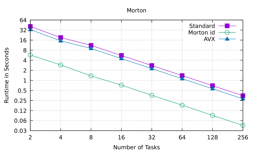
Figure 2: Strong scaling results for Morton (Algorithms 1, 4 and 11) in various quadrant implementations. The raw Morton implementation gives a 77% average performance boost and AVX2 gives 17% in comparison to the standard quadrant implementation.

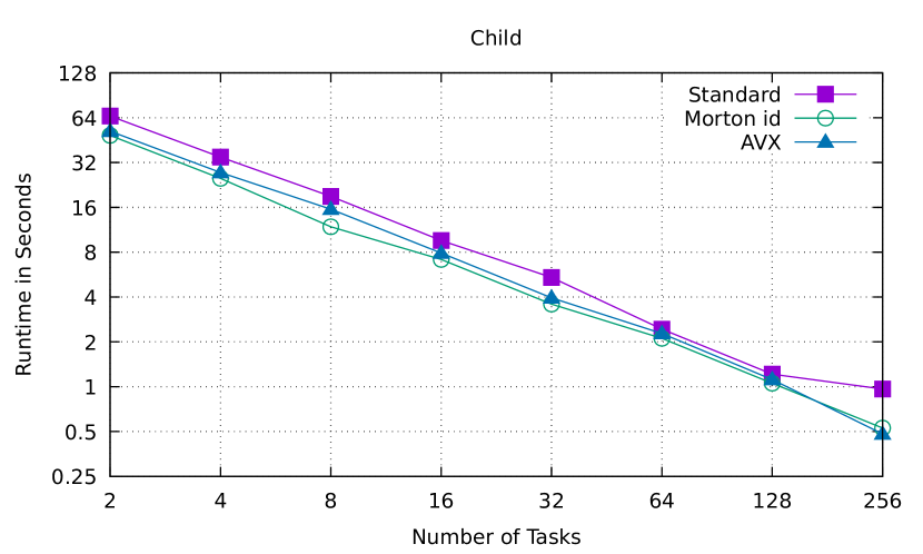
Figure 3: Strong scaling results for Child (Algorithms 2, 6 and 9) in various quadrant implementations. The raw Morton implementation gives 20% while AVX2 gives a 29% average performance boost.

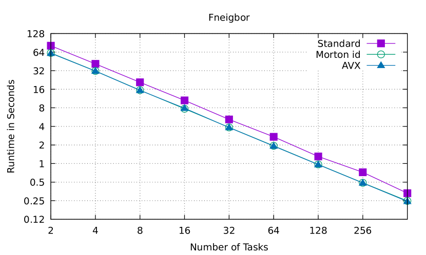
Figure 4: Strong scaling results for FNeigh (e.g. Algorithm 8) in various quadrant implementations. The raw Morton implementation gives 26% while AVX2 gives a 27% average performance boost.

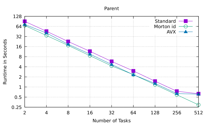
Figure 5: Strong scaling results for Parent (e.g. Algorithms 7 and 10) in various quadrant implementations. The raw Morton implementation gives 27% while AVX2 gives a 15% average performance boost in comparison to the standard implementation.

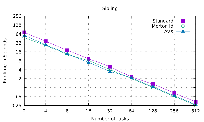
Figure 6: Strong scaling results for Sibling (e.g. Algorithm 3) in various quadrant implementations. The raw Morton implementation gives 23% while AVX2 gives a 21% average performance boost.

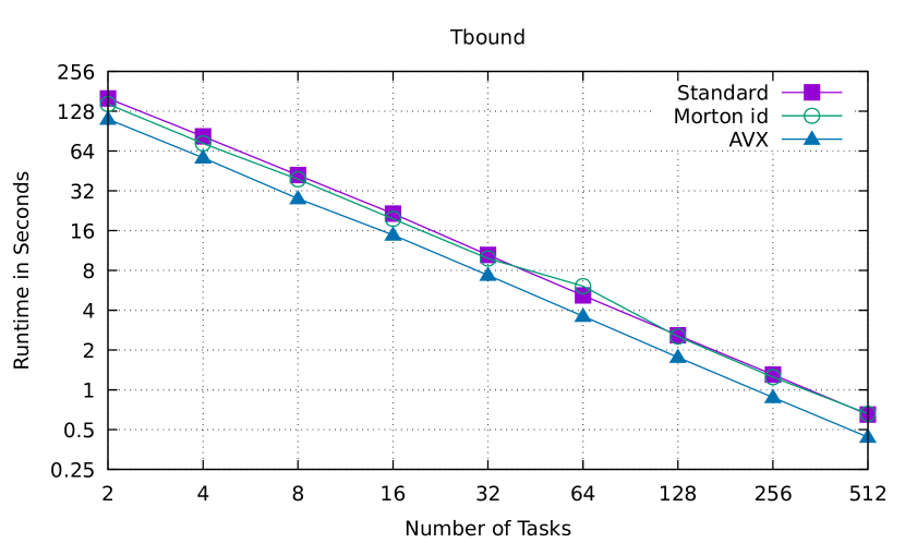
Figure 7: Strong scaling results for Tree_Boundaries (i.e. Algorithm 12) in various quadrant implementations. The raw Morton implementation gives 3% while AVX2 gives a 31% average performance boost.

Overall, both new quadrant implementations show speed-ups comparing to the standard one. The Morton, Child and Parent algorithms perform faster for the raw Morton index than for AVX2 quadrants; see Figures 2, 3 and 5. Conversely, FNeighbor and Parent make no difference in terms of efficiency for both new representations (see Figures 4 and 6), while Tree_Boundaries works faster with quadrants processed with 128-bit AVX2 instructions, which is demonstrated by Figure 7.

3.2 Comparison of memory consumption.

We compare the amount of memory consumed by the program operating on the various representations of quadrants. Our software prescribes the following memory for each quadrant implementation in 3D:

• standard quadrants consisting of three 32-bit coordinates, 8 bits for level, 24 bits padding and 64 bits of user data. It consumes 24 bytes of memory in total.

• The raw Morton index representation as described in Section 2.2 requires one 64-bit integer variable equal to 8 bytes of memory.

• Quadrants stored in extended 128-bit SSE/AVX2 registers as described in Section 2.3 take 16 bytes.

We utilize a memory consumption preset of the Intel VTune Profiler software, measuring the memory required to build a uniform octree of level 10 using repeated calls to the Morton algorithm to obtain the following results: the program allocates 25.8 GB for standard, 17.2 GB for AVX and 8.6 GB for Morton quadrants. The ratio 3:2:1 between these values is as expected.

4 Conclusion

In this paper we describe two new representations of quadrants in the context of the adaptive mesh refinement library p4est, namely a single raw Morton index long integer and a 128-bit SSE/AVX2 representation, respectively. We present the specific ways the quadrants are encoded for each representation and detail several low-level algorithms operating on them. Arguably, the new algorithms are both less intuitive and more intricate than those based on the standard representation using explicit $xyz$ coordinates.

Our tests demonstrate a performance boost over the standard for both new types of implementation. In most of them a raw Morton index shows better results than quadrants processed by 128-bit SSE/AVX2 instructions, but in some cases the Morton representation requires to make the algorithm more complex, which leads to slowing down the performance.

Both new implementations require less RAM for quadrant storage while keeping the maximum refinement level the same (18 for the raw Morton index in 3D) or allowing it to be higher (31 for the SSE/AVX2 implementation). We note however that the standard implementation has since caught up to a maximum level of 29 in 3D, and its 8 bytes of payload might be removed for a memory consumption on par with AVX2. Based on these facts, a user can choose their favorite implementation of a quadrant depending on the required performance, resolution, and resources on the one hand and simplicity and continuity on the other.

We consider several directions for the future. The first one is the straightforward use of a wider register capacity, for example 256-bit registers from AVX2 or 512 bits provided by AVX-512. The practically reachable resolution can then be increased even further, while the necessity of a refinement level beyond 30 is admittedly somewhat unclear. The second is the integration of a raw Morton index implementation with extended 128-bit CPU registers. This will combine the advantages of both new implementations: lesser complexity of some algorithms and higher maximum refinement level in general. Moreover, the use of one 128-bit register will still have equal RAM requirements than AVX2 or the standard implementation without payload.

To make the new algorithms accessible through the p4est software, we have been working on a new branch of high-level algorithms that operate on virtualized quadrants. Presently we cannot predict whether the new interface and glue code will be acceptable to the community, or if the way forward will rather be to wait for a portable compiler support of 128 bit CPU registers and to hardcode the appropriate updates into the internals of the software.

References

- [1] M. Bader, C. Böck, J. Schwaiger, and C. Vigh, Dynamically adaptive simulations with minimal memory requirement—solving the shallow water equations with Sierpinski curves, SIAM Journal of Scientific Computing, 32 (2010), pp. 212–228.
- [2] W. Bangerth, C. Burstedde, T. Heister, and M. Kronbichler, Algorithms and data structures for massively parallel generic adaptive finite element codes, ACM Transactions on Mathematical Software, 38 (2011), pp. 1–28.
- [3] C. Burstedde, p4est: Parallel AMR on forests of octrees, 2010. https://www.p4est.org/ (last accessed January 24th, 2023).
- [4] , Parallel tree algorithms for AMR and non-standard data access, ACM Transactions on Mathematical Software, 46 (2020), pp. 1–31.
- [5] C. Burstedde and J. Holke, A tetrahedral space-filling curve for nonconforming adaptive meshes, SIAM Journal on Scientific Computing, 38 (2016), pp. C471–C503.
- [6] C. Burstedde, L. C. Wilcox, and O. Ghattas, p4est: Scalable algorithms for parallel adaptive mesh refinement on forests of octrees, SIAM Journal on Scientific Computing, 33 (2011), pp. 1103–1133.
- [7] M. J. Flynn, Some computer organizations and their effectiveness, IEEE Transactions on Computers, C-21 (1972), pp. 948–960.
- [8] I. Hadade, F. Wang, M. Carnevale, and L. di Mare, Some useful optimisations for unstructured computational fluid dynamics codes on multicore and manycore architectures, Computer Physics Communications, 235 (2019), pp. 305–323.
- [9] J. Holke, C. Burstedde, D. Knapp, L. Dreyer, S. Elsweijer, V. Ünlü, J. Markert, I. Lilikakis, N. Böing, P. Ponnusamy, and A. Basermann, t8code v. 1.0 – modular adaptive mesh refinement in the exascale era, in SIAM International Meshing Round Table 2023, Amsterdam, NL, March 2023, SIAM.
- [10] J. Holke, D. Knapp, and C. Burstedde, An optimized, parallel computation of the ghost layer for adaptive hybrid forest meshes, SIAM Journal on Scientific Computing, 43 (2021), pp. C359–C385.
- [11] Intel Corporation, Intel 64 and IA-32 architectures optimization reference manual, 2019. https://software.intel.com/sites/default/files/managed/9e/bc/64-ia-32-architectures-optimization-manual.pdf, last accessed on June 30th, 2020.
- [12] T. Isaac, C. Burstedde, and O. Ghattas, Low-cost parallel algorithms for 2:1 octree balance, in Proceedings of the 26th IEEE International Parallel & Distributed Processing Symposium, vol. 1, IEEE, 2012, pp. 426–437.
- [13] T. Isaac, C. Burstedde, L. C. Wilcox, and O. Ghattas, Recursive algorithms for distributed forests of octrees, SIAM Journal on Scientific Computing, 37 (2015), pp. C497–C531.
- [14] T. Isaac and M. G. Knepley, Support for non-conformal meshes in PETSc’s DMPlex interface, 2015. http://arxiv.org/abs/1508.02470.
- [15] S. Jubertie, F. Dupros, and F. De Martin, Vectorization of a spectral finite-element numerical kernel, in Proceedings of the 2018 4th Workshop on Programming Models for SIMD/Vector Processing, WPMVP’18, New York, NY, USA, 2018, Association for Computing Machinery.
- [16] S. Keller, A. Cavelan, R. Cabezon, L. Mayer, and F. Ciorba, Cornerstone: Octree construction algorithms for scalable particle simulations, in Proceedings of the Platform for Advanced Scientific Computing Conference, PASC ’23, New York, NY, USA, 2023, Association for Computing Machinery.
- [17] D. Knapp, Adaptive Verfeinerung von Prismen, Bachelor’s thesis, Rheinische Friedrich-Wilhelms-Universität Bonn, 2017.
- [18] , A space-filling curve for pyramidal adaptive mesh refinement, Master’s thesis, Rheinische Friedrich-Wilhelms-Universität Bonn, 2020.
- [19] G. M. Morton, A computer oriented geodetic data base; and a new technique in file sequencing, tech. rep., IBM Ltd., 1966.
- [20] A. Müller, M. A. Kopera, S. Marras, L. C. Wilcox, T. Isaac, and F. X. Giraldo, Strong scaling for numerical weather prediction at petascale with the atmospheric model NUMA, The International Journal of High Performance Computing Applications, (2018), p. 1094342018763966.
- [21] J. Rudi, A. C. I. Malossi, T. Isaac, G. Stadler, M. Gurnis, P. W. J. Staar, Y. Ineichen, C. Bekas, A. Curioni, and O. Ghattas, An extreme-scale implicit solver for complex PDEs: Highly heterogeneous flow in earth’s mantle, in Proceedings of the International Conference for High Performance Computing, Networking, Storage and Analysis, SC ’15, New York, NY, USA, 2015, Association for Computing Machinery.
- [22] B. M. Shabanov, A. A. Rybakov, and S. S. Shumilin, Vectorization of high-performance scientific calculations using avx-512 intruction set, Lobachevskii Journal of Mathematics, 40 (2019), pp. 580–598.
- [23] H. Sundar, R. Sampath, and G. Biros, Bottom-up construction and 2:1 balance refinement of linear octrees in parallel, SIAM Journal on Scientific Computing, 30 (2008), pp. 2675–2708.
- [24] H. Tropf and H. Herzog, Multidimensional range search in dynamically balanced trees, Angewandte Informatik, 2 (1981), pp. 71–77.
- [25] T. Tu, D. R. O’Hallaron, and O. Ghattas, Scalable parallel octree meshing for terascale applications, in SC ’05: Proceedings of the International Conference for High Performance Computing, Networking, Storage, and Analysis, ACM/IEEE, 2005, pp. 4–4.
- [26] T. Weinzierl and M. Mehl, Peano—a traversal and storage scheme for octree-like adaptive Cartesian multiscale grids, SIAM Journal on Scientific Computing, 33 (2011), pp. 2732–2760.