Number-State Reconstruction with a Single Single-Photon Avalanche Detector: Supplemental Material

Abstract

This is a supplementary document to Number-State Reconstruction with a Single Single-Photon Avalanche Detector. Here we discuss details of the detector matrix construction as well as the methodology and uncertainty budgets for the characterization of our detectors.

A Construction of the Detector Matrix

As discussed in the main text, a pulse of light with photon-number distribution $\mathbf{P}$ under repeated measurements produces a click number distribution $\mathbf{C}$. All of the effects of the detector are contained in a matrix relating the two:

$$\mathbf{C}=\mathbb{D}\mathbf{P}.$$ (1)

In turn, in our model $\mathbb{D}$ is composed of four matrices:

$$\mathbb{D}=\mathbb{A}(p_{a})\mathbb{R}[\gamma(t),D(\tau)]\mathbb{B}(p_{B})\mathbb{L}(\eta_{0}),$$ (2)

where each of these matrices encodes the effects of a particular SPAD imperfection. In this section we detail the methods we use to construct these matrices. We have made the code that implements everything in this section open-access, as well as provided some sample data and example reconstruction implementations, available in Code 1 [1].

A.I Detection Efficiency

The simplest, and typically largest, correction to be applied to the click distribution to reach the incident photon number distribution is the non-unit detector efficiency (DE). If the detector is fully armed when a photon arrives, then the probability of generating a click is a Bernoulli process; thus if all of the photons of a pulse arrive when the detector is fully armed, the probability that a given number of clicks is produced is

$$P(\text{$m$ clicks given $n$ photons})={n\choose m}\eta_{0}^{m}(1-\eta_{0})^{n-m},$$ (3)

where $\eta_{0}$ is the DE when the detector is fully armed. Note that the binomial coefficient is zero when $m>n$. From the above equation, we define the matrix $\mathbb{L}(\eta_{0})$ through its elements $\mathbb{L}_{mn}(\eta_{0})$, which are the probabilities that, of $n$ incident photons, $m$ produce clicks and $n-m$ are lost. Note that $\mathbb{L}(\eta_{0})$ is upper triangular.

A.II Background Counts

We model background counts, including dark counts, as a Poisson process [2] with a total rate $r_{b}$, which we take to be constant over the data collection time scale. Thus if a data collection window has duration $T$, then the mean number of background events is $p_{b}=r_{b}T$. The probability of $k$ background events is then

$$P(\text{$k$ background counts})=\frac{p_{b}^{k}e^{-p_{b}}}{k!}.$$ (4)

We use this to construct the background count matrix $\mathbb{B}(p_{b})$, whose elements $\mathbb{B}_{mn}$ are the probabilities that there will be $m-n$ background counts in the data collection window, so that $n$ photon-produced clicks yield $m$ total (photon-produced and background) clicks. Since background counts add to the total counts, this matrix is lower triangular. Note also that since background counts add clicks, the possible total number of clicks is unbounded. Therefore truncating the basis produces probabilities whose sum differs from one. We manually set $\mathbb{B}_{n_{\text{max}}n}$, the last row of the matrix, so that each column sums to unity.

A.III Recovery Time Effects

The construction of the recovery time effects matrix $\mathbb{R}$ requires detailed consideration, because recovery time effects are correlated with previous clicks, and this memory has to be taken into account.

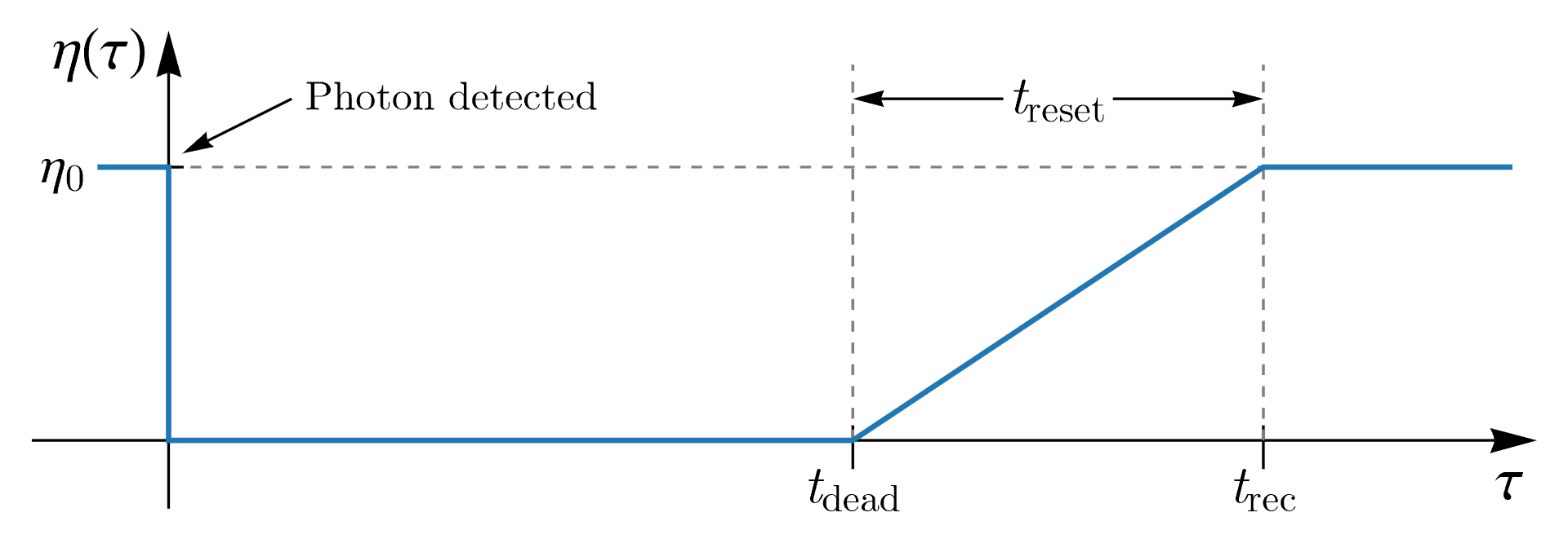
Figure 1: Illustration of our model of SPAD recovery effects [3]. The function $\eta(\tau)$ is the efficiency of the detector immediately following a photon detection, with $\eta_{0}$ being the fully armed efficiency. After a photon arrives and causes an avalanche ($\tau=0$), the detector becomes dead for a time $t_{\text{dead}}$ set by the quenching circuit. The circuit then resets the bias over a time $t_{\text{reset}}$ and the detector starts to be able to sense photons. The total time to return to full bias is the recovery time $t_{\text{rec}}=t_{\text{dead}}+t_{\text{reset}}$. We define $D(\tau)=1-\eta(\tau)/\eta_{0}$ as the loss profile.

When a fully armed detector clicks, the system efficiency changes due to the action of the quenching circuit. We model this behavior with an efficiency function $\eta(\tau)$ shown in Fig. 1. (Although it is possible to measure $\eta(\tau)$ [4], we simply assume the model here.) For this piece of the formalism, we want to correct for recovery time effects only, so we use a scaled version of $\eta(\tau)$, namely $D(\tau)=1-\eta(\tau)/\eta_{0}$, a function that is zero if the detector loses no clicks to recovery time effects and 1 if it has no ability to click due to recovery time effects. Using this function treats all losses as caused by the dead time.

Additionally, let $\gamma(t)$ be the input photon profile. We measure $\gamma$ by histogramming the arrival times of the clicks in only the runs where exactly one click occurred, and normalizing the histogram. As discussed below, this is an approximation and suffers from distortions due to recovery time and afterpulsing effects, but these distortions are generally small, and often a separate measurement can be made to reduce their effects. This measured profile also includes background counts, but this is desirable, since the combination of background and photon counts is what we model to be affected by the dead time.

With this paradigm, imagine an experimental run in which two photons are incident on the detector. According to the above discussion, we assume the first photon generates a click. Then there are three possibilities for the second photon, enumerated in Table 1:

1. It arrives during the recovery time triggered by the previous click, and gets lost (i.e. does not produce a click);

2. It arrives during the recovery time of the previous click, and produces a click, which is delayed until the end of the recovery time (note that these are twilight counts [4]);

3. It arrives after the recovery time of the first photon, and therefore produces a click, since the detector has recovered and is fully armed.

The probabilities of each of these events can be calculated using $\gamma(t)$ and $D(\tau)$ as:

$$p_{1} =\frac{1}{N_{2}}\int_{0}^{T}\gamma(t_{1})\int_{t_{1}}^{t_{1}+t_{\text{rec}}}\gamma(t_{2})D(t_{2}-t_{1})\,dt_{2}\,dt_{1},$$ (5)

$$p_{2} =\frac{1}{N_{2}}\int_{0}^{T}\gamma(t_{1})\int_{t_{1}}^{t_{1}+t_{\text{rec}}}\gamma(t_{2})[1-D(t_{2}-t_{1})]\,dt_{2}\,dt_{1},$$ (6)

$$p_{3} =\frac{1}{N_{2}}\int_{0}^{T}\gamma(t_{1})\int_{t_{1}+t_{\text{rec}}}^{T}\gamma(t_{2})\,dt_{2}\,dt_{1}.$$ (7)

Here $T$ is the data collection time duration and $N$ is a normalization factor,

$$N_{2}=\int_{0}^{T}\gamma(t_{1})\int_{t_{1}}^{T}\gamma(t_{2})\,dt_{2}\,dt_{1}.$$ (8)

The second integral in each equation is a factor that determines the probability of the relevant event given that a photon arrived at time $t_{1}$, and $\gamma(t_{1})$ is the probability that the first photon arrives at time $t_{1}$. We then integrate over the arrival time of the first click. Note that $\gamma(t)$ does not have to be a true probability density in the sense of integrating to unity; the normalization factor $N_{2}$ handles this. By inspection, $p_{1}+p_{2}+p_{3}=N_{2}/N_{2}=1$. Note that, when $\gamma(t)$ does integrate to 1 over the window from $t=0$ to $t=T$, we get $N_{2}=1/2$, consistent with an identical particles formulation of the problem.

For higher numbers of incident photons, the possible combinations of the three types of events grows quickly, and at high count rates all of these possibilities have to be considered. Thus, to treat large Fock bases, we need an algorithm that determines all of the possibilities and the necessary integrals. In the following, we detail (a) an encoding method for photon events, (b) an algorithm for generating all possible events, (c) an algorithm for constructing the needed integral for each event, and finally (d) the method for including the result of the integral in the recovery effects matrix $\mathbb{R}$.

Table 1: Summary of photon events for calculating recovery effects. The detector may be fully armed or recovering, and if the latter the photon may or may not produce a click, resulting in three different event types for every photon that arrives at the detector. This table also gives the symbol for encoding each possible event and a justification for the symbol. Note that in the accompanying Code 1 [1], these symbols are replaced with (from top to bottom) 1, 2, and 3.

Description of event	Symbol	Symbol explanation
Photon arrives during the recovery time triggered by the previous click, and gets lost (i.e. does not produce a click)	$\circ$	A circle is used for photons arriving while the detector is recovering; the hollow circle indicates the loss of the photon.
Photon arrives during the recovery time triggered by the previous click, and itself produces a click, which is delayed until the end of the recovery time (i.e. a twilight count)	$\bullet$	A circle is used for photons arriving while the detector is recovering; the filled circle indicates the photon produces a click.
Photon arrives when the detector is fully armed (i.e. after the recovery times of all previous clicks), and therefore produces a click	$\bigstar$	The star indicates this photon is different from other events in that it arrives when the detector is fully armed.

Encoding.

We begin by coding all possible combinations of the three types of events. Every experimental run contains a set of photons, each of which arrived in one of the three conditions described in Table 1. Thus we can describe the photons of any run by a string of symbols encoding the arrival conditions of each photon, in order of arrival. We use the symbols $\circ$, $\bullet$, and $\bigstar$, as mapped and justified in Table 1.

In writing down all possible events, we assume the first photon of a run arrives when the detector is in normal operating mode, i.e. the first photon is always a $\bigstar$. This is a good assumption when there is no signal prior to the start of the detection window.

For example, the string $\bigstar\bullet$ describes a run in which the first photon arrives when the detector is fully armed and produces a click, and then a second photon arrives within the first click’s recovery time and produces a delayed twilight count. And $\bigstar\circ\bullet$ is an experimental run in which the first photon produces a click because it arrives when the detector is fully armed, and then the second photon arrives during that first click’s recovery time and is lost, and then a third photon arrives, also during the first click’s recovery time, and produces a delayed twilight count.

There is one more factor to determining possible events, which we can see by considering the string $\bigstar\bullet\bullet$. When a $\bullet$ appears in the string, a photon arrived during the recovery time of the previous click, and generated a new, delayed click. But this formulation means the string $\bigstar\bullet\bullet$ has an ambiguity of interpretation: either (a) both of the $\bullet$ photons arrived during the recovery time of the same click (the first of the cycle), or (b) the second photon arrived during the recovery time of the first click, and produced a new click, and then the third photon arrived during the recovery time of that second click. In the first case, note that the three photons produce only two clicks total, but in the second case all three photons produce a click. There are many strings with similar ambiguities.

To disambiguate these possibilities, we add square brackets $\left[\leavevmode\nobreak\ \right]$ to our strings. These brackets indicate photons that come in the same recovery periods, and we refer to the photons grouped by these brackets simply as “groups.” For example, scenario (a) in the previous paragraph will be written $\left[\bigstar\bullet\bullet\right]$ (one group), while (b) will be written $\left[\bigstar\bullet\right]\left[\bullet\right]$ (two groups). We use the term “event” to refer to a specific, unambiguous set of photon events, and the term “event string” to refer to the encoding of the event, while we use the term “string” to refer simply to a possible combination of $\circ$’s, $\bullet$’s, and $\bigstar$’s with no grouping. For more than two incident photons, typically one string (like $\bigstar\bullet\bullet$) corresponds to more than one event, like the two written above.

Note that $\bigstar$ photons require no disambiguation, so long as we enforce the definition: a $\bigstar$ happens only after all previous recovery times have finished. This means $\bigstar$ photons are always at the beginning of their group (though not all groups begin with a $\bigstar$). For instance possible events include $\left[\bigstar\bullet\right]\left[\bigstar\right]$ and $\left[\bigstar\bullet\right]\left[\bigstar\circ\right]$. In addition, $\circ$ photons require no disambiguation, as they produce no click, and therefore do not affect the detector dynamics.

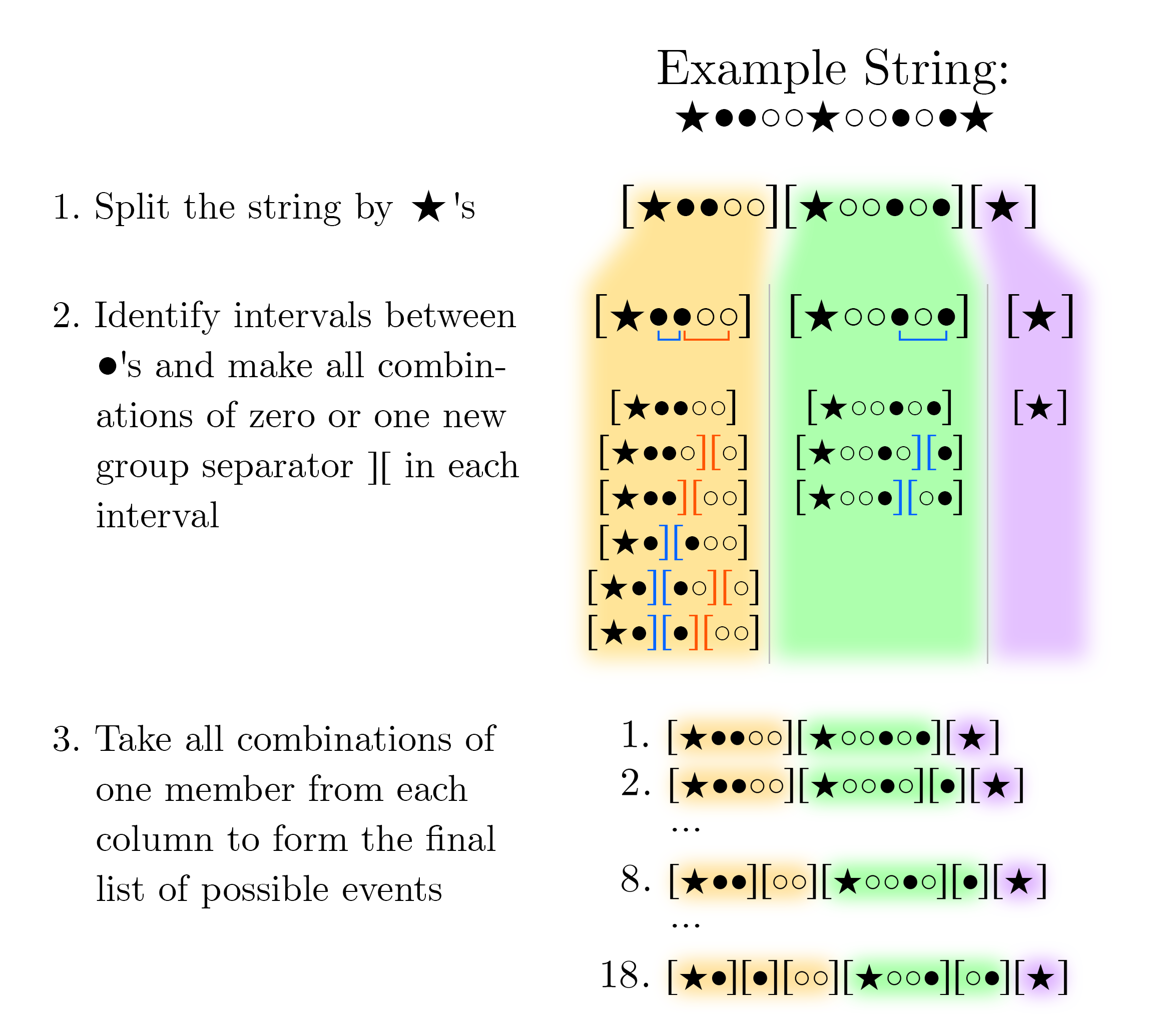
Figure 2: An illustration of the algorithm for generating all possible events corresponding to a given string, using an example string to show the process.

Generating Possible Events.

Using this encoding, we can discuss how to generate possible events. A first step is to form all possible combinations of up to $n_{\text{max}}$-symbol strings of $\bigstar$, $\bullet$, and $\circ$ which begin with a $\bigstar$. (Here $n_{\text{max}}$ is the largest $n$ considered in the truncated basis.) For each of these strings, we generate the set $S$ of possible events. The general algorithm for doing this is illustrated for an example string in Fig. 2. Starting with a given string and the empty set $S$, there are three basic steps:

1. Split the string by $\bigstar$’s, so that each substring begins with exactly one $\bigstar$. This splitting corresponds to the definition: when a $\bigstar$ occurs, it means all previous recovery times have finished.

2. Account for the ambiguities caused by $\bullet$’s: for each substring, find $\bullet$’s. Generate new events using the rule that, between every $\bullet$ in the substring and the next $\bullet$ in that substring (or the end of the substring), there may be no additional splittings, or there may be exactly one additional split $][$ between any two photons. This generates a set of possible events $S_{i}$ for the photons of each group from step 1, where $i$ indexes the substrings from Step 1.

3. The set $S$ of possible events for the entire string is generated by forming all possible combinations of exactly one member of each of the sets $S_{i}$ and concatenating the choices, in order.

Performing this algorithm on all combinations of $\circ$’s, $\bullet$’s, and $\bigstar$’s up to length $n$ results in a set of all possible events of up to $n$ photons.

Constructing the Integral for an Event.

Each of the events from the algorithm above is a possible experimental realization with an occurrence probability, which we compute by performing integrals over $\gamma(t)$.

As each photon arrives at a time $t_{i}$, and these times are integrated over, $t_{i}$ become integration variables. Since each photon must come after the previous photon, the integrals are nested such that an inner integral in general depends on the previous $t_{i}$. There are three things to be determined for each of the integrals: the integral bounds, the integrand, and, if the integrand includes a $D$ function, the argument of that $D$ function.

For the integrand, the rules are: for a $\bigstar$, integrate over $\gamma$ only; for a $\circ$, integrate over $\gamma D$; and for a $\bullet$, integrate over $\gamma(1-D)$. The argument of $\gamma$ is always the arrival time of the photon (the integration variable). The argument of $D$ will be the integration variable minus some “reference” time, which is the time of the previous click. Algorithmically we can determine the reference time as follows:

• If the photon is preceded by another $\circ$ or $\bullet$ in the same group, use the same reference as the $D$ function in the previous integral, because this photon arrived during the recovery time of the same click as the last photon.

• If the photon is at the beginning of a group or is preceded by a $\bigstar$, the reference should be the start of the integral, because this photon is the first one to arrive in this recovery time.

The integral bounds are set as follows. For the start of the integral,

1. The very first photon’s integral starts at $t=0$.

2. If the photon is a $\circ$ or $\bullet$ that is not at the beginning of its group, use the previous integral’s integration variable as the start time.

3. If the photon is a $\circ$ or $\bullet$ at the beginning of its group, use the time of the previous $\bigstar$ plus $nt_{\text{rec}}$, where $n$ is the number of group separators $][$ between the last $\bigstar$ and the current photon.

4. If the photon is a $\bigstar$, look to the most recent photon that is not a $\circ$. If that photon is a $\bigstar$, start the integral at the time of that $\bigstar$ plus $t_{\text{rec}}$. If that photon is a $\bullet$, start the integral at the time of the time reference of the $D$ function of the $\bullet$’s integral plus $2t_{\text{rec}}$, leaving an extra recovery time for the click produced by the $\bullet$.

Finally, for the end of the integral,

1. If the photon is a $\circ$ or $\bullet$ that is not at the beginning of its group but is not immediately preceded by a $\bigstar$, use the previous integral’s end time.

2. If the photon is a $\circ$ or $\bullet$ that is at the start of its group, or is not at the start of its group but is immediately preceded by a $\bigstar$, end the integral $t_{\text{rec}}$ after the integral’s start time.

3. If the photon is a $\bigstar$, end the integral at $T$.

We note here that these integral bounds imply a simplifying assumption, namely that all twilight counts come at exactly the end of the recovery time of the previous click, with no spread in time. Although it is possible to measure the spread of delays of twilight counts [4] and account for it, we do not do so here.

After the integral is constructed according to the above rules, it needs to be divided by the normalization factor

$$N_{m}=\int_{0}^{T}\gamma(t_{1})\int_{t_{1}}^{T}\gamma(t_{2})\cdots\int_{t_{m-1}}^{T}\gamma(t_{m})\,dt_{m}\cdots\,dt_{1}.$$ (9)

where $m$ is the number of photons in the event.

We give a few examples of higher-order integrals, which together demonstrate all of the rules given in this section:

$$\left[\bigstar\bullet\circ\right] : p=\frac{1}{N_{3}}\int_{0}^{T}\gamma(t_{1})\int_{t_{1}}^{t_{1}+t_{\text{rec}}}\gamma(t_{2})[1-D(t_{2}-t_{1})]\int_{t_{2}}^{t_{1}+t_{\text{rec}}}\gamma(t_{3})D(t_{3}-t_{1})\,dt_{3}\,dt_{2}\,dt_{1}$$

$$\left[\bigstar\bullet\right]\left[\circ\right] : p=\frac{1}{N_{3}}\int_{0}^{T}\gamma(t_{1})\int_{t_{1}}^{t_{1}+t_{\text{rec}}}\gamma(t_{2})[1-D(t_{2}-t_{1})]\int_{t_{1}+t_{\text{rec}}}^{t_{1}+2t_{\text{rec}}}\gamma(t_{3})D(t_{3}-(t_{1}+t_{\text{rec}}))\,dt_{3}\,dt_{2}\,dt_{1}$$

$$\left[\bigstar\circ\right]\left[\bigstar\right] : p=\frac{1}{N_{3}}\int_{0}^{T}\gamma(t_{1})\int_{t_{1}}^{t_{1}+t_{\text{rec}}}\gamma(t_{2})D(t_{2}-t_{1})\int_{t_{1}+t_{\text{rec}}}^{T}\gamma(t_{3})\,dt_{3}\,dt_{2}\,dt_{1}$$

$$\left[\bigstar\bullet\right]\left[\bigstar\circ\right] : p=\frac{1}{N_{4}}\int_{0}^{T}\gamma(t_{1})\int_{t_{1}}^{t_{1}+t_{\text{rec}}}\gamma(t_{2})[1-D(t_{2}-t_{1})]\int_{t_{1}+2t_{\text{rec}}}^{T}\gamma(t_{3})\int_{t_{3}}^{t_{3}+t_{\text{rec}}}\gamma(t_{4})D(t_{4}-t_{3})\,dt_{4}\,dt_{3}\,dt_{2}\,dt_{1}$$

Contributing to the Matrix.

Finally, the integral for each event is interpreted as a probability that a given number of photons results in a particular number of clicks. Therefore each integral is a contribution to some element of the matrix $\mathbb{R}$. For each event, the number of photons, and therefore the column of the element to add the integral result to, is simply the total number of $\circ$’s, $\bullet$’s, and $\bigstar$’s in the event’s string. The number of clicks, which determines the row of the matrix element to add the integral to, is the number of groups in the event string, with one additional caveat to correctly include twilight counts:

1. For each $\bigstar$, look for the closest previous photon that is not a $\circ$. If it is a $\bullet$, and that $\bullet$ is in the group immediately preceding the $\bigstar$, then add one to the total number of clicks.

2. If there is a $\bullet$ after the last $\bigstar$ of the entire event string, and this $\bullet$ is in the last group of the string, add one to the total number of clicks.

For instance, the string $\bigstar\bullet\circ\bullet\bullet$ codes to six events, all of which have five photons. The event $\left[\bigstar\bullet\circ\bullet\bullet\right]$ has two clicks, the events $\left[\bigstar\bullet\circ\bullet\right]\left[\bullet\right]$, $\left[\bigstar\bullet\circ\right]\left[\bullet\bullet\right]$, and $\left[\bigstar\bullet\right]\left[\circ\bullet\bullet\right]$ have three clicks, and $\left[\bigstar\bullet\circ\right]\left[\bullet\right]\left[\bullet\right]$ and $\left[\bigstar\bullet\right]\left[\circ\bullet\right]\left[\bullet\right]$ have four clicks, the maximum possible number for this string (the $\circ$ is guaranteed to be lost).

By combining all of this—producing strings that code possible events, using those strings to construct the integrals for the probabilities of those events, and then evaluating those integrals and adding the results to the appropriate elements of the matrix—we produce the recovery effects matrix $\mathbb{R}$.

We note that, if all possible events for a basis of a given size are computed, the columns of the matrix should sum to unity, as the integrals for $p_{1}$, $p_{2}$, and $p_{3}$ did. However, in practice one may want to reduce the time taken to compute the matrix when it is known that the recovery time effects are not too large, e.g. for low count rates. In this case one can save time by implementing an “order” parameter $o_{R}$, which is defined such that at most $o_{R}$ photons can arrive during the recovery times of all clicks. (It is so named because it indicates what is typically meant by the “order” of the calculation.) This is equivalent to reducing the initial set of all $\circ$’s, $\bullet$’s, and $\bigstar$’s to just the set containing at most $o_{R}$ $\circ$’s and $\bullet$’s (and any number of $\bigstar$’s). When $o_{R}$ is less than the size of the matrix, we partially populate the first $o_{R}$ diagonals of $\mathbb{R}$ above the true diagonal, but we do not compute all possible events, so the columns do not add to one. We fix this manually, in the following way: for each column $n$, if $n-o_{R}\leq 1$, all events in the column have been calculated and the column should already be normalized, but if $n-o_{R}>1$, we set the element in row $n-o_{R}-1$ of the column so that the column sums to one. (Here rows and columns are zero-indexed.) This corresponds physically to approximating that all the uncalculated events fall into the first uncalculated order of corrections. The effects of $o_{R}$ on the reconstruction of an input pulse whose recovery time effects are significant are shown in Fig. 3.

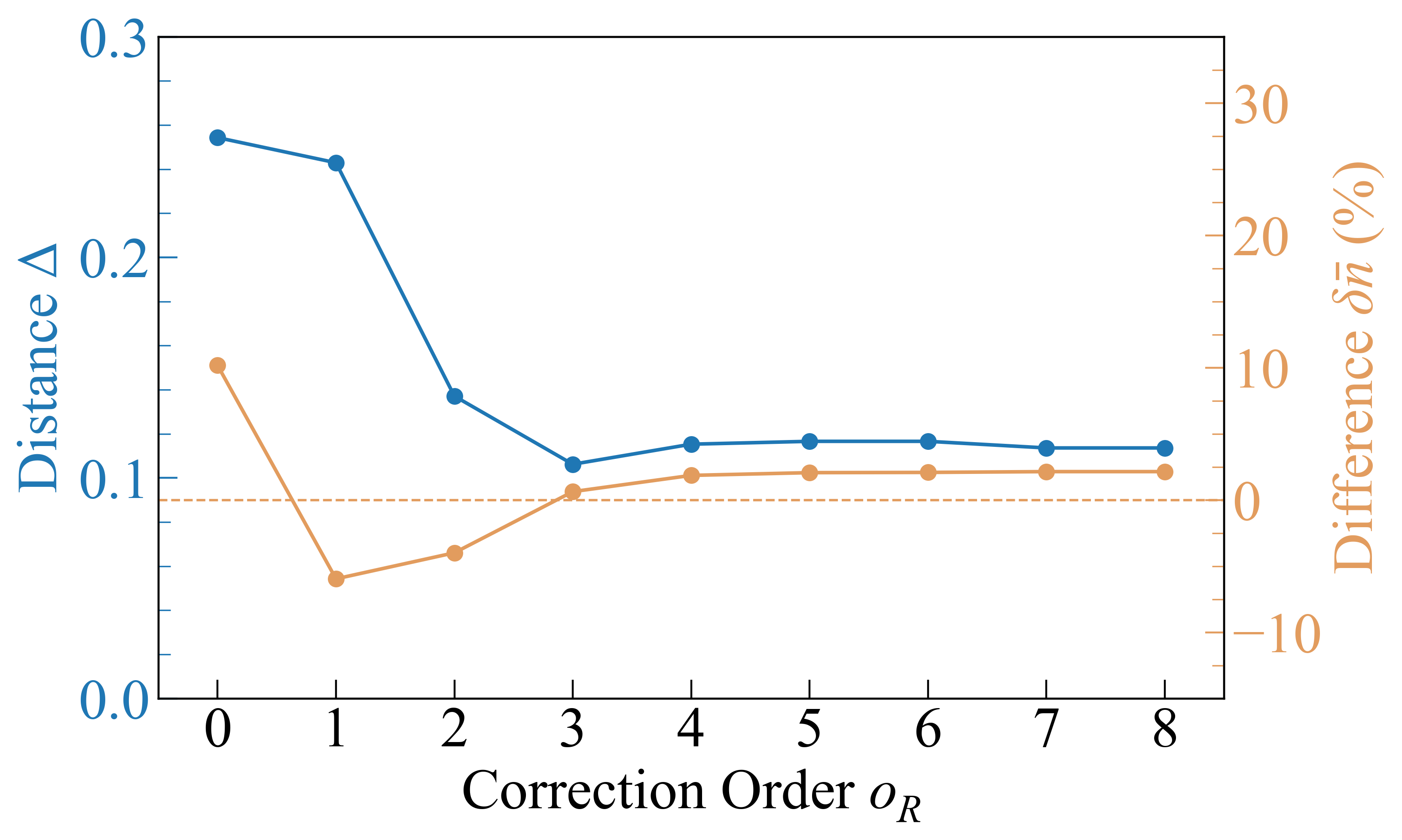
(a)

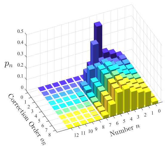
(b)

Figure 3: A demonstration of the reconstruction of the short (85 ns full-width half-max) pulse of Fig. 4(c2) of the main text, which had an input average photon number $\bar{n}_{\text{fit}}=3.97$, or about one photon per recovery time. In this limit the recovery time effects are large, and the calculation must be taken to high orders. The 3D bar plot shows the reconstructions as a function of the order parameter $o_{R}$. For low $o_{R}$, the fraction of photons put into low numbers varies somewhat with $o_{R}$; meanwhile there is no population at high numbers, because recovery time effects mean we almost never observe events with more than a few clicks, and $o_{R}$ is not large enough that the matrix $\mathbb{R}$ can “add back” those clicks. But as $o_{R}$ is increased, the matrix gains more power to add back clicks, and also results in a distribution that is stable to changes in $o_{R}$. The inset on the left shows the convergence of both the total variation distance $\Delta$ and the difference $\delta\bar{n}$ as we increase $o_{R}$.

A.IV Afterpulsing Effects

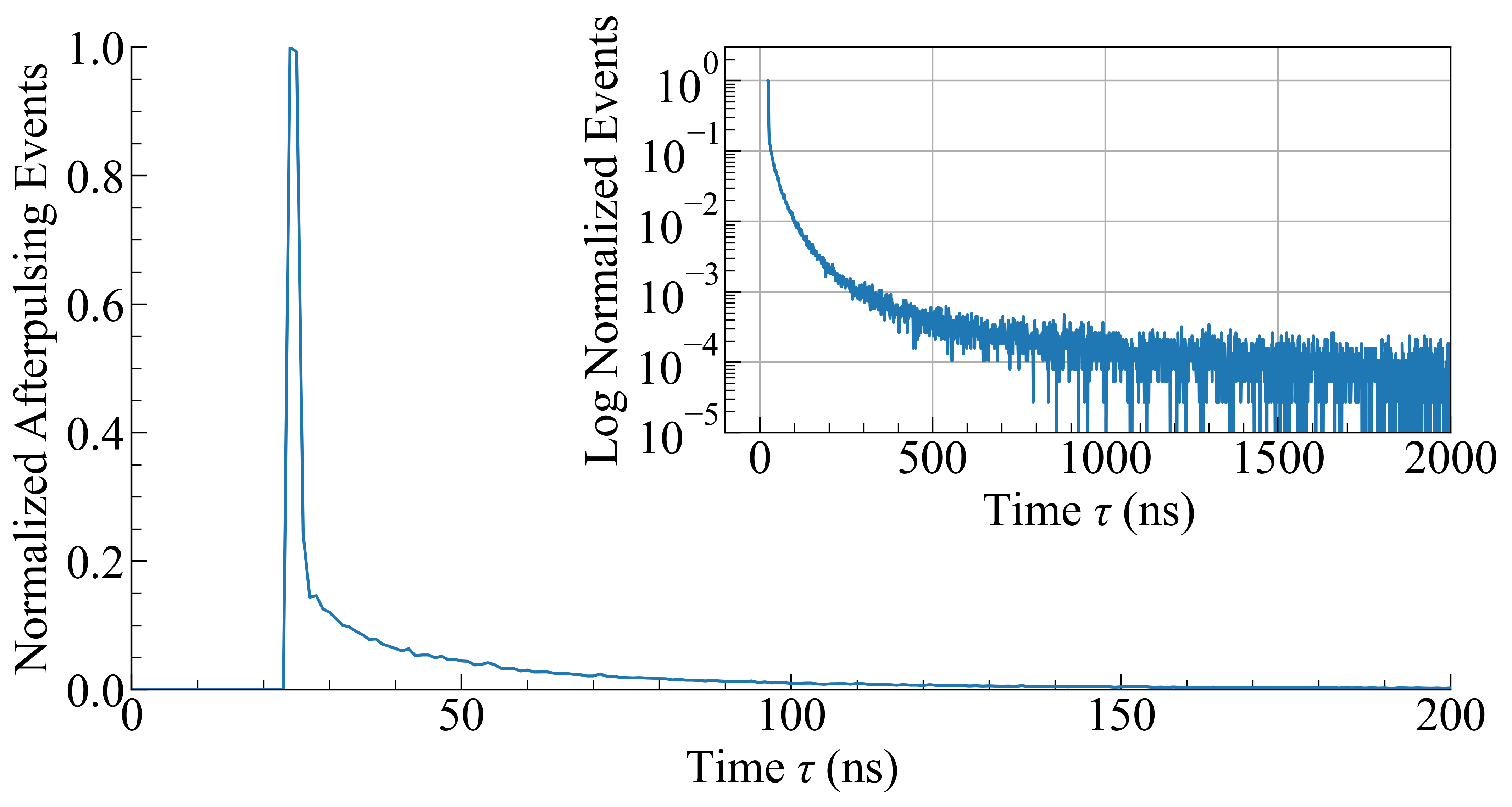
Figure 4: A measured afterpulsing profile. The main figure shows the details of the first 200 ns of afterpulsing, which contains 87.3 % of the afterpulsing feature. The inset shows, on a log scale, the first 2 $\mu$s of the afterpulsing, showing the common hyperexponential-like behavior [5]. The first 2 $\mu$s contain 94.8 % of the afterpulsing feature for this detector, SPAD2. The counts have been normalized here for simplicity, but this detector is measured to have about 2.4 % total afterpulsing probability. Note the initial period of zero events, which is the due to the recovery time of the detector. Our methodology for retrieving the afterpulsing profile and probabilities is described in Section B.

We correct for afterpulsing by finding the probability $p_{a}$ of one afterpulse occurring in our data collection window, and use this to generate all afterpulsing corrections. To find $p_{a}$, we convolve the time-dependent afterpulsing probability with the photon profile. As an example of why this is necessary, consider performing reconstruction on a light pulse that fits inside a 2 $\mu$s data collection window, using a SPAD that has the afterpulsing profile of Fig. 4. If a click occurs at the beginning of the window, it has a 2.3 % chance of afterpulsing within the window; if the click occurs 1.8 $\mu$s into the window, it drops to 2.1 % . To account for this, we convolve the time profile $a(\tau)$ with the photon profile. This gives the probability of an afterpulse click in the data collection window as:

$$p_{a}=\int_{0}^{T}\gamma(t)\int_{t}^{T}a(t^{\prime}-t)\,dt^{\prime}\,dt.$$ (11)

where $T$ is the data collection window duration. We use this probability to generate the afterpulsing matrix $\mathbb{A}(p_{a})$. The elements of $\mathbb{A}$ relate a number of “real” clicks (clicks caused by signal photons or by background events) to total (“real” plus afterpulsing) clicks.

Given the above, we need to calculate the probability that $m$ real counts generate $n$ afterpulses, giving $m+n$ total clicks. Any particular click may afterpulse or not with probabilities $p_{a}$ and $1-p_{a}$ respectively. Thus the probability that a click generates zero afterpulses is $1-p_{a}$. Then the probability that a click generates exactly one afterpulse is $p_{a}(1-p_{a})$, because the original click afterpulses, but the afterpulse click does not afterpulse. Proceeding in this way, the probability of a click producing $n\geq 0$ afterpulses is $p_{a}^{n}(1-p_{a})$.

Using the above model and assumptions, we determine the probability that $m$ real clicks generate $n$ total afterpulses. We can think of grouping the $n$ afterpulses into $m$ groups, each of which can have inclusively between 0 and $n$ of the afterpulse clicks. For instance, two real counts may produce three afterpulses in four ways: the first click may afterpulse three times and the second one none, the first click twice and the second once, the first click once and the second twice, or the first click none and the second click three times. This example may make clear that we can formulate the problem by asking the ways that exactly $m$ nonnegative integers can sum to $n$. For the previous example, $m=2$ and $n=3$ sees the possible sums $3+0$, $2+1$, $1+2$, $0+3$. An analytical expression for the number of sums is not known to the authors, but it can be computed numerically.

From these sums we can determine the contribution to the probability of $m$ real clicks producing $n$ afterpulses. Each sum identified above contributes a term to be summed to obtain the final expression. Every term has the same form: they are the product of $m$ factors of $(1-p_{a})$ and $n$ factors of $p_{a}$. The number of sums available from the reasoning of the previous paragraph only determines the number of such factors and therefore a prefactor for each element of $\mathbb{A}$. For example, the probability that two real clicks produce three afterpulses, which is the matrix element $\mathbb{A}_{52}$ since there are five total clicks from two real clicks, is

$$\mathbb{A}_{52}=4\times(1-p_{a})^{2}p_{a}^{3}.$$ (12)

In this way we can build up the entire afterpulsing matrix.

If desired, in practice one can limit the number of afterpulses accounted for by implementing an “order” parameter $o_{a}$, which we define as the maximum number of afterpulses that can be produced by all of the clicks in a single experimental run. A finite $o_{a}$ merely places a limit on the maximum distance from the diagonal for which we will compute matrix elements. For all the reconstructions in this work, we use $o_{a}=2$.

Because afterpulsing adds clicks, the possibilities for events are infinite: a single real click can produce two total clicks, or three, or four, and so on. Since the matrices we compute are always finite, the computed probabilities will never sum to unity. This is true regardless of the chosen order parameter $o_{A}$. To resolve this, we manually set elements as follows: for each column $n$, if $n+o_{a}+1\geq n_{\text{max}}$, set the element in row $n_{max}$, and otherwise, set the element in row $n+o_{a}+1$ such that the column sums to one. Physically this corresponds to letting all of the uncalculated probabilities fall into the next order of the calculation.

A.V Limitations of the Model

The model and calculations presented here involve a number of approximations, which we discuss in this section, in no particular order.

Afterpulsing models.

We note that we have not carefully considered the physical mechanisms of the afterpulsing in our SPADs, which may impact the probability distribution used for the calculation. The model we have used, in which the probability of $n$ afterpulses is geometric, is widely adopted, but the use of a Poissonian distribution is equally reasonable from arguments about the density and number of these traps [6, 7]. Such a model appears to produce larger total variation distances for our detectors.

Calculation of the photon profile.

Both the afterpulsing probability calculation and the calculation of the recovery time effects matrix $\mathbb{R}$ require a photon profile $\gamma(t)$ over which to integrate, but our measured click profiles are affected by dead times and afterpulsing. We have approximated $\gamma(t)$ by histogramming the clicks in data collection cycles where the detector registers exactly one click. This choice suffers from some distortions, e.g. if a photon impinges on the detector and produces a click, and then a second photon arrives while the detector is dead, the run is counted as producing only one click, even though there were two photons.

When the input light state is Poissonian, these effects may be analyzed and corrected by modeling the process as a Poisson point process [6]. Consider an input state with a mean photon rate $\lambda(t)$, and define $\Lambda(t_{1},t_{2})=\int_{t_{1}}^{t_{2}}\lambda(t)\,dt$. The survival probability, the probability of no detections, from $t=0$ to later time $t$ is $e^{-\Lambda(0,t)}$. The probability of the first detection is

$$p_{1}(t_{1})=\lambda(t_{1})e^{-\Lambda(0,t_{1})}.$$ (13)

The probability of this being the only detection in the window from $t=0$ to $t=T$ is the probability of one detection at $t_{1}$ multiplied by the probability of no further detections, $e^{-\Lambda(t_{1},T)}$, so that the probability of exactly one click in window $T$ is

$$P_{1}(t_{1})=\lambda(t_{1})e^{-\Lambda(0,T)}.$$ (14)

If our detector were ideal, $P_{1}$ would be proportional to $\lambda(t_{1})$ and we could use it directly to measure the photon profile. However, for instance, a dead time $t_{d}$ modifies the single click probability to $P_{1}^{\prime}(t_{1})=\lambda(t_{1})e^{-\Lambda(0,t_{1})}e^{-\Lambda(t_{1}+t_{d},T)}$, no longer proportional to $\lambda(t_{1})$ [6].

For coherent states, an improvement to the model can be made by numerically solving Eqn. 13. Analysis of our coherent-state data shows only negligible improvements, even for large count rates. For non-coherent states, the use of Eqn. 13 is incorrect. For instance, if the pulse is a pure two-photon Fock state, we will not recover the full photon profile by only looking at single-click experimental cycles. One solution is to take a separate measurement in which a large attenuation is placed in front of the detector; this should make the entire pulse shape accessible while leaving it unchanged.

Model of the recovery time; non-Markovianity of afterpulsing and recovery time.

In this work we assume a model for the quantum efficiency during the recovery time shown in Fig. 1. We note that this property of the detector can actually be measured using, for instance, the methods of Ref. [4], in which very short light pulses are sent to the detector with controlled delays and the resulting detector response is measured.

Our model of the detector during the recovery time loses validity at high count rates, as discussed further below and shown in Fig. 7. There could be numerous reasons for this due to the non-Markovian behavior of the detector, which is not modeled in our algorithm. This behavior manifests in various ways. (1) Changes to the recovery time with increasing count rate have been observed [8]. In our data we observe a shift of the DEP by around 0.5 ns occurring around count rates of 10 Mcounts/s. This increase is not accounted for in our model. (2) When a twilight count occurs, the quenching circuitry of the SPAD is not activated in the typical manner, and a result of this may be that the avalanche current lasts longer than usual [8]. The deep traps that later result in afterpulsing may get more filled than usual, resulting in an afterpulsing probability that increases with count rate. (3) It has also been shown that each avalanche fills only a small number of the total deep traps in a diode, so that as the count rate increases, it is reasonable to imagine more of these traps getting filled, resulting again in an afterpulsing probability that increases as the count rate increases [7].

Correlations in the recovery time effects matrix.

To write down the integral equations for calculating the various probabilities in the recovery time effects matrix $\mathbb{R}$, we make an assumption about the joint photon arrival time probability, namely that $\lambda(t_{1},t_{2},\dots,t_{n})=\lambda(t_{1})\lambda(t_{2})\cdots\lambda(t_{n})$. This is really only true for Poissonian light; in general, correlations in the light lead to correlations in the detections [9].

It can be shown, either from a semiclassical or a fully quantum theory, that the probability density of a first photodetection is [9]

$$P_{1}(t)\,dt=\alpha I(t)\,dt$$ (15)

where $\alpha$ is a constant related to detector properties. From this, the joint probability density of two photodetections is [9]

$$P_{2}(t_{1},t_{2})\,dt_{1}\,dt_{2}=\alpha^{2}\langle:I(t_{1})I(t_{2}):\rangle\,dt_{1}\,dt_{2}=\alpha^{2}P_{1}(t_{1})P_{2}(t_{2})g^{(2)}(t_{1},t_{2})\,dt_{1}\,dt_{2}$$ (16)

where we have introduced the normalized second-order autocorrelation function $g^{(2)}$. Thus when $\langle:I(t_{1})I(t_{2}):\rangle\ \neq\langle I(t_{1})\rangle\langle I(t_{2})\rangle$, or when $g^{(2)}(t_{1},t_{2})\neq 1$, we cannot write $P_{2}(t_{1},t_{2})=P_{1}(t_{1})P_{1}(t_{2})$. Arguments of this type generalize to larger numbers of photodetections as well [9].

This algorithm might be improved for non-Poissonian light by constructing a more detailed mathematical theory including correlations. However, with a single detector, the correlation information that is available is subject to all of the detector imperfections, especially afterpulsing and dead times. For instance, with just one detector with a dead time, there is simply no way to measure $g^{(2)}(t_{1},t_{2})$ when $t_{2}-t_{1}$ is less than the dead time.

This is one reason that the pulses being measured with this algorithm must have widths and correlations at least a few detector dead times in length; when this condition is satisfied, the error made by this approximation is small, because the recovery time effects matrix only changes the reconstructed number-state distribution for events that occur during the recovery time. In general, this approximation will push the reconstructed distribution toward a Poissonian distribution.

Interactions of afterpulses and twilight counts.

This model does not include “interactions” between afterpulses and recovery time effects as seen by the detector. Although afterpulses have an independent physical origin from recovery time effects, their occurrence on the same detector causes them to interact in important ways. Afterpulsing does not occur when the detector is dead. Thus, afterpulses due to previous clicks may be prevented by subsequent clicks, which becomes more likely when the count rate is high. Large count rates also change the temporal distribution of the afterpulsing. After a click, twilight counts and afterpulsing have temporal profiles which overlap (in the few nanoseconds immediately after the recovery time), but the detector can only register one of them. When the there is a significant probability of a twilight count, the likelihood of an afterpulse is reduced.

As discussed in the main text, we believe the fact that our algorithm does not address these interactions is the primary limitation at the highest count rates. At high count rates the DEP clicks are overcompensated, pushing the fitted average photon number per pulse below what is expected and producing reconstructed distributions that are narrower than the corresponding Poissonian.

B Detector Calibration Techniques

In this section, we discuss our methodology for measuring all of the inputs to our SPAD model.

B.I Using Second-Order Histograms

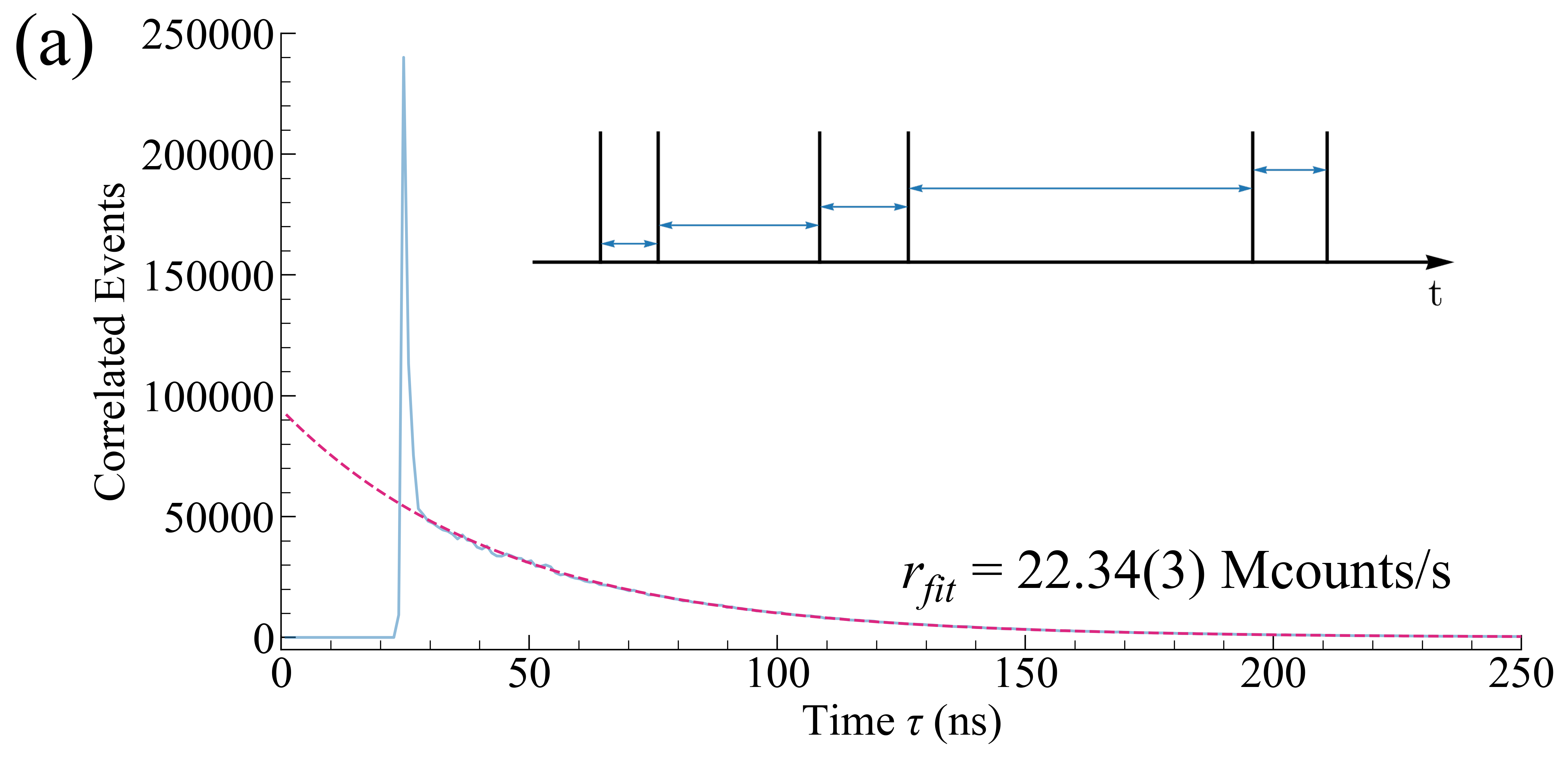
(a)

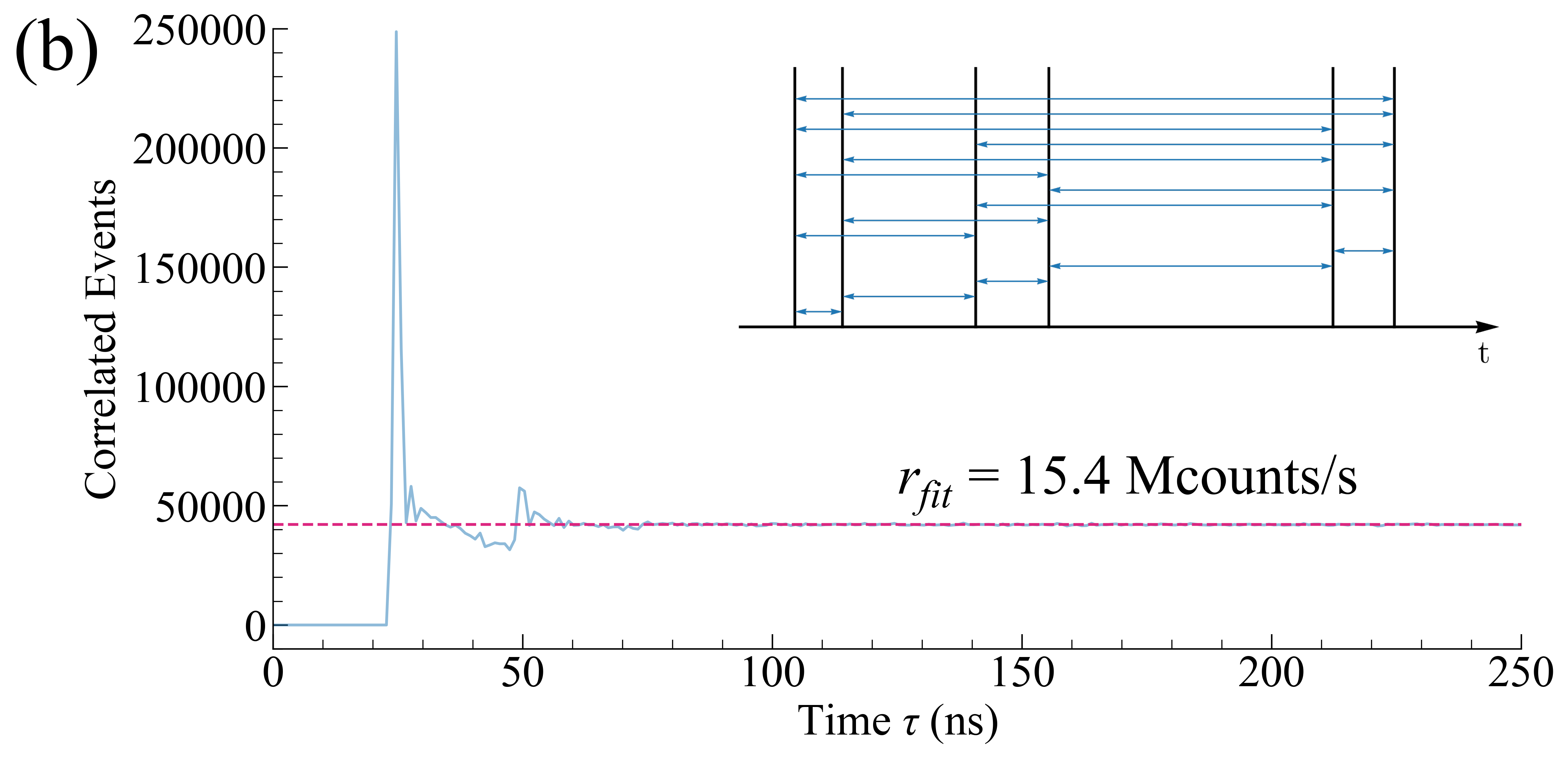
(b)

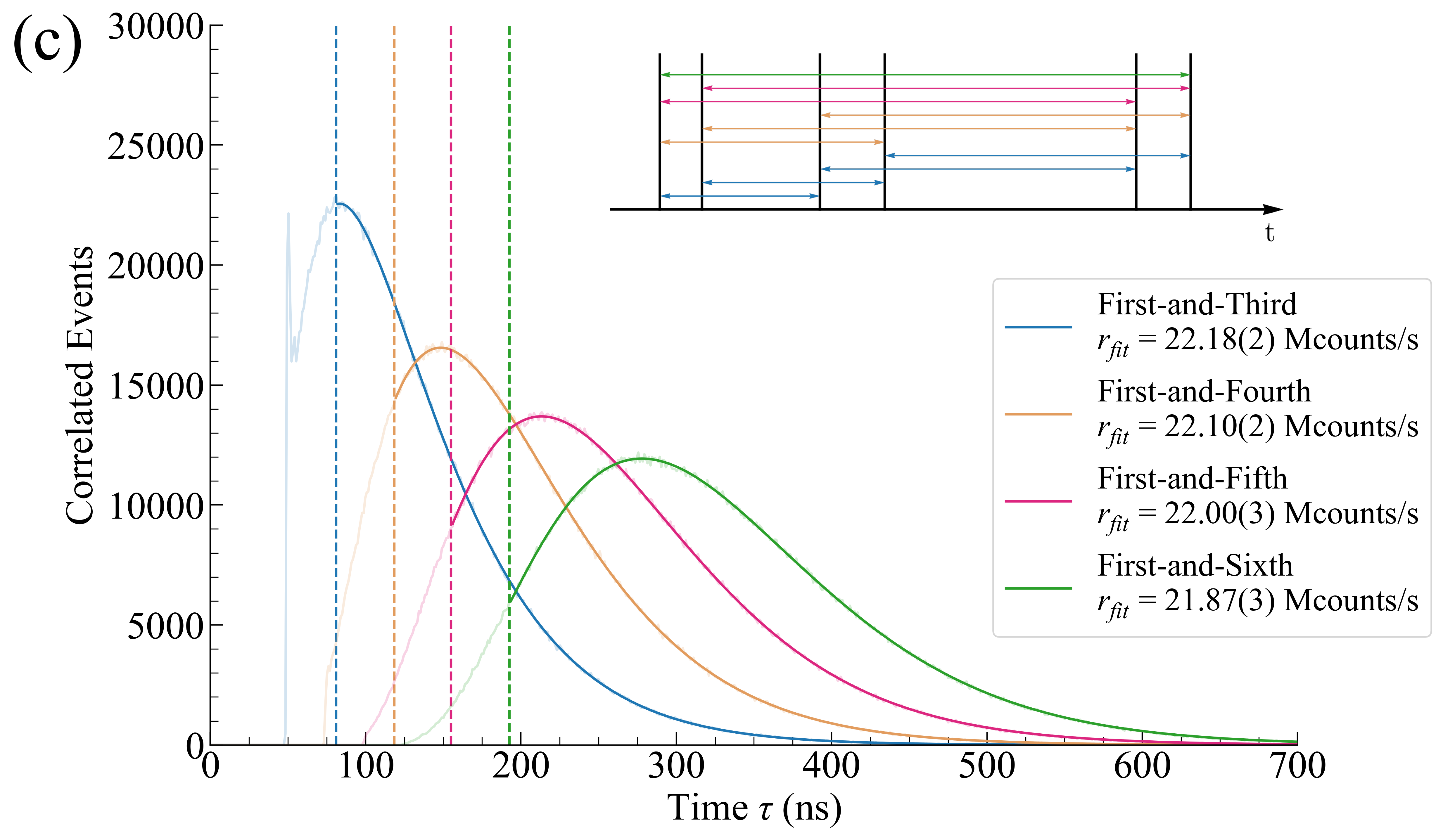
(c)

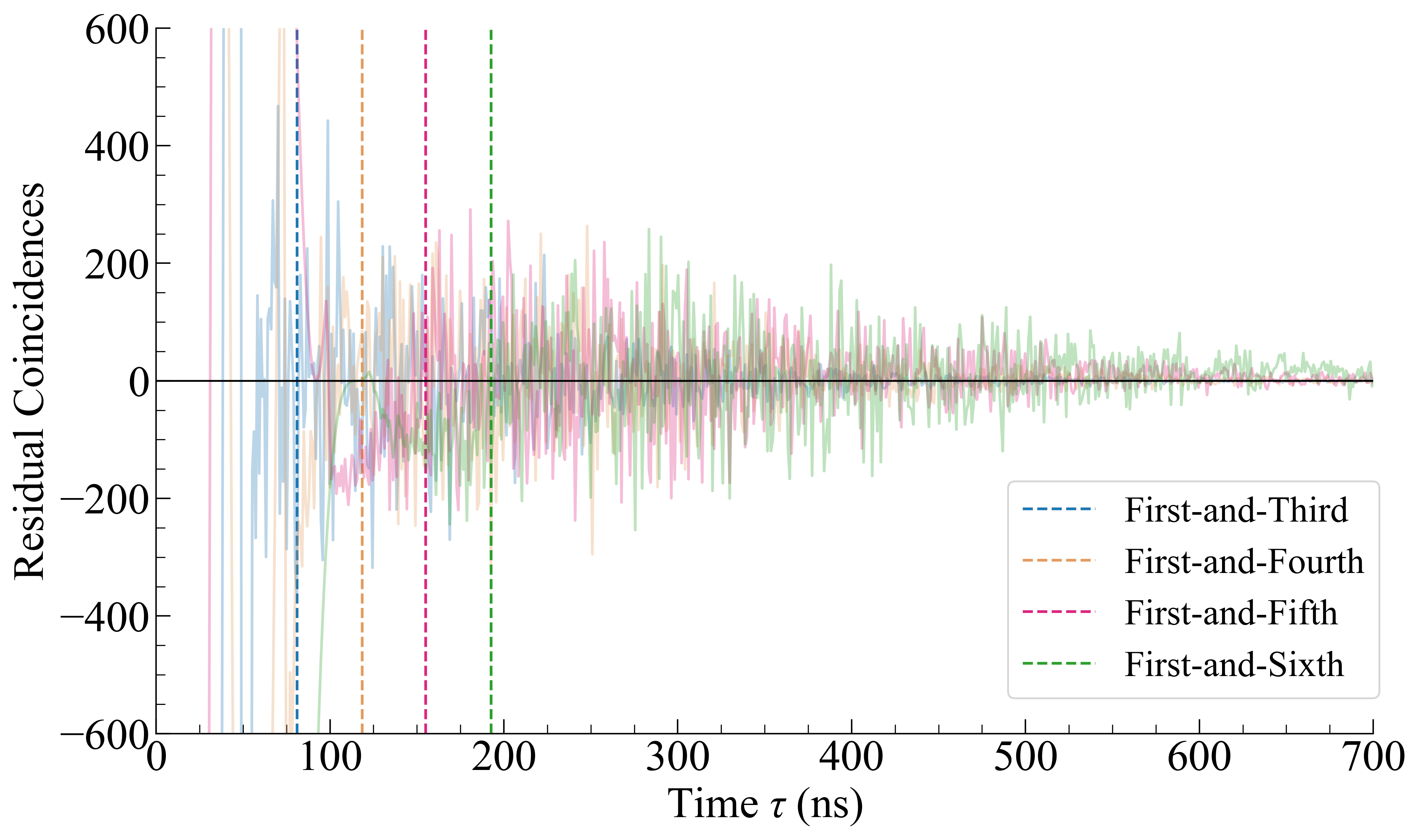
(d)

Figure 5: Various second-order histograms generated from the same dataset, with $\approx$ 30 Mcounts/s of cw input light. In (a,b,c), the insets illustrate the click pairs used to generate the respective histograms; the horizontal axis is a time axis, and the thick vertical lines represent times when clicks occur. Pairs of clicks connected by arrows are included in the histogram, and the connecting arrows are color-coded to match the respective main figures. (a) First-and-second or “interarrival” data (blue) shows an exponential behavior (dashed magenta) after the detector effects peak (DEP). The fitted count rate using Eqn. 19 is 22.34(3) Mcounts/s. (b) Full second-order correlation data (blue) shows a linear behavior (dashed magenta) after the DEP. The fitted count rate (starting the fit at 100 $\mu$s) is 15.4 Mcounts/s, altered heavily by recovery time losses. The long-time behavior of this type of histogram is a linear function whose x-intercept is the data collection time. (c) Left panel: First-and-$n$ histograms for $3\leq n\leq 6$, with solid fit lines overlaying the data. Fitted count rates using Eqn. 19 from $n=3$ to $n=6$ are as indicated in the legend: 22.18, 22.10, 22.00, 21.87 Mcounts/s, a difference of up to 2.2 % from the first-and-second fit. The vertical dashed lines indicate the times at which each fit is begun. Right panel: Residuals from the fits shown in the left panel, with a notable lack of structure at times greater than the fit start time, shown again with vertical dashed lines.

Most of the calibration analysis involves the generation of various second-order histograms of times between pairs of clicks, with the only difference being which pairs of clicks to include. These histograms are used for various functions in the calibration analysis, but one of the most important is the extraction of detected count rates. Count rates are extracted from second-order histograms by fitting the histogram data to a theoretical lineshape, which is not exactly what is observed due to the time-correlated recovery time and afterpulsing effects. In this subsection we discuss several types of second-order histograms, as shown in Fig. 5, along with the theoretical lineshapes and effects of detector imperfections on each type, and how we use each type in our detector characterization.

One type of second-order histogram is first-and-second histogram (Fig. 5a) is a histogram of waiting times between clicks that are adjacent in time. This type of data has often been called “interarrival data” in the literature, and it is the the most common second-order histogram to produce because it has historically been the easiest type of data to gather, using relatively simple click-time processing circuits. These histograms plot the probability that no click occurs for a time $\tau$ after an initial click, and then a click occurs at time $\tau$ after the initial event. This is why the histogram in Fig. 5a is zero for the first $\approx$ 25 ns: this is the recovery time, where photons that arrive are either lost altogether, or their clicks are delayed until later as twilight counts. The large peak immediately after the recovery time is what we call the “detector effects peak” (DEP), and it contains both afterpulsing clicks and twilight counts. While twilight counts have a fairly narrow distribution, afterpulsing may extend tens of microseconds as shown partially in Fig. 4 (which is also a first-and-second histogram). After this time, the detector fully recovers, and the histogram faithfully reproduces the statistics of the input light.

For Poissonian light, once the detector has recovered from previous clicks, the shape of the histogram should fit $e^{-r\tau}$, which is the Poisson probability of no events for a time $\tau$ followed by one event at that time. Since we can fit this exponential using an independent amplitude parameter, the $r$ here is unaffected by dead-time losses, which only scale the histogram. However, this type of data suffers from a crucial problem: the afterpulsing feature has an exponential-like shape on a first-and-second histogram, so to avoid this feature affecting the fitted count rate, we must fit data at large delays. But when the count rate is large, one has to wait a very long time to gather data at large $\tau$. In our SPADs, afterpulsing is noticeable for tens of $\mu$s, so let us suppose we wait for 100 $\mu$s to avoid afterpulsing. In this example, at even a very modest continuous count rate of 100 kcounts/s, the probability of no click for at least 100 $\mu$s (assuming no afterpulsing) is about $4.5\times 10^{-5}$, so that one needs to wait more than six hours on average before getting a single event beyond 100 $\mu$s. Thus, building statistics sufficient for a two-parameter exponential fit without the influence of afterpulsing is impractical. (We do, however, use first-and-second histograms in other ways, as discussed in the next section.)

Another choice is to generate full second-order correlation data, which is a histogram of the delays between all pairs of clicks in a dataset. Such a histogram is shown in Fig. 5b. This data still exhibits the sharp afterpulsing peak, and we observe the effects of this peak for tens of $\mu$s, so we fit to data beginning at a delay of 100 $\mu$s. But because we look at all pairs of clicks in this data, the extent of delays for which we can easily get data is much larger; in fact the largest delay for which there is a histogrammed event is necessarily equal to the data collection time. For Poissonian light, there is a constant probability of a click, so the probability for a particular delay between clicks (with any number of events in between) is also constant. Because we only collect data for a finite amount of time, experimentally the shape we see (if we view the entire dataset, not shown in Fig. 5b) is a downward-sloped line whose $x$-intercept is equal to the data collection time. The downward slope (a deviation from the theoretically horizontal line) is purely an edge effect. The shape of the histogram at large delays is given by $r^{2}\Delta t(t_{0}-t)$, where $t_{0}$ is the total data collection time and $\Delta t$ is the bin width. A fit to this line is shown as the magenta dashed line in Fig. 5b. We can think of the expression as a product of $r\Delta t$, the probability of a click per bin, and $r(t_{0}-t)$, which captures the number of clicks “available” for correlations at time $t$ in the data collection. Note the nature of the extracted $r$: it is only an amplitude in the mathematical expression. Since these histograms are scaled by dead time losses as discussed above, the extracted count rate is decreased by dead time losses. The typical correction factor for such an effect is

$$r^{\prime}=\frac{r}{1-rt_{D}},$$ (17)

where $t_{D}$ is the dead time and $r^{\prime}$ would be the measured count rate if there were no dead time. In this work we do not rely on count rates extracted this way, but full second-order correlation data is used in other ways, as discussed further below.

A final type of second-order histogram is higher-$n$ first-and-$n$ histograms, which plot the delays between each click and the $(n-1)$th click immediately after it. (First-and-second histograms are a special case of these, with $n=2$.) Fig. 5c shows several of these histograms generated from the same dataset. A first-and-$n$ histogram is a measure of the probability of having exactly $n-2$ clicks in a time $t$. For Poissonian light on an ideal detector, these events follow a probability density function that is $p_{n}^{\text{ideal}}(t)=(rt)^{n-2}e^{-rt}/(n-2)!$. For a detector that has a recovery time $\tau_{r}$ and a probability $p_{a}$ of an afterpulse or twilight count occurring immediately at the end of the recovery time, it can be shown [6] that the probability density function for times beyond the recovery time is

$$p_{n}(t)=re^{-r[t-(n-1)\tau_{r}]}\sum_{k=1}^{n-1}{n-1\choose k}p_{a}^{n-1-k}(1-p_{a})^{k}\frac{r^{k-1}\left[t-(n-1)\tau_{r}\right]^{k-1}}{(k-1)!},\hskip 10.00002ptt>\tau_{r},n\geq 2.$$ (18)

(This is Eqn. S24 of Ref. [6], with $\tau_{i}$ set to equal $\tau_{r}$ to model the fact that first-and-$n$ histograms assume a click at $t=0$.) The $k=n-1$ term with $\tau_{r}=0$ and $p_{a}=0$ corresponds to the ideal detector expression. While the ideal detector expression already produces a good fit to data, Monte Carlo simulations suggest that the fitted count rates vary from the true count rates by amounts on the order of 1-2%, and there is a deviation from the true count rate depending on the portion of the histogram used for fitting. However, it can be shown using Eqn. 18 that, to first-order in $p_{a}$, the number of events per bin is

$$P_{n}(t) =N\Delta t\,r\left[1-(n-1)p_{a}+\frac{(n-1)(n-2)p_{a}}{r(t-(n-1)\tau_{r})}\right]\frac{\left[r(t-(n-1)\tau_{r})\right]^{n-2}}{(n-2)!}e^{-r(t-(n-1)\tau_{r})},$$ (19)

$$\hskip 320.00049ptt>\tau_{r},n\geq 2.$$

The factor $N\Delta t$ converts the probability density into a number of events per bin, with $N$ the number of clicks in the dataset and $\Delta t$ the width of the time bin used to discretize the data. Eqn. 19 is an expression being fit for $r$, $p_{a}$, and $\tau_{r}$, with no independent amplitude parameter. It uses the same assumptions as Eqn. 18, but drops higher-order terms in $p_{a}$, which makes the fit more numerically robust. The term proportional to $p_{a}/rt$ biases the histogram slightly to early times; this corresponds to the fact that, when an $n$-click sequence involves an afterpulse, the average duration of the sequence will be shorter since afterpulses have a timescale shorter than that of the average time between photon-produced clicks. The term proportional to $p_{a}$ then scales down the entire histogram to make up for this addition, renormalizing the probability density function.

In using Eqn. 19 we make two notes. First, $p_{a}$ and $\tau_{r}$ empirically have a large covariance, so we constrain $\tau_{r}$ by setting it equal to the time of the first nonzero bin in the histogram. Second, $p_{a}$ has only some relation to the “true” afterpulsing+twilight probability. The above equations model these phenomena as occurring immediately after the end of the recovery time, which results in maximum distortion of the histogram toward early times; to the extent that afterpulsing and twilight counts have any temporal width in a real detector, this distortion is reduced, so we expect the fitted $p_{a}$ to be lower than the true $p_{a}$. We see this empirically in using Eqn. 19. As a result, we generally discount the fitted value of $p_{a}$ and measure the afterpulsing+twilight probability in other ways, as discussed below. We note also that, while the fitted $p_{a}$ has a somewhat large uncertainty in our fits, the covariance between $p_{a}$ and $r$ is small, so the fitted count rate is robust to this uncertainty.

From Monte Carlo simulations, Eqn. 19 gives nearly constant fitted count rates regardless of where the fitting is begun, as long as it is at delays of at least two recovery times. Furthermore, these simulations suggest that, for $n\geq 4$, the fitted count rate is below but well within 1% of the true rate, and that this fitted rate converges as $n$ increases and improves with both smaller $p_{a}$ and afterpulsing that has greater temporal width. That is, we can fit nearly the entire histogram, without regard to the limit of 100 $\mu$s set for avoiding afterpulsing, and still achieve very good fitted count rates. To our knowledge, this technique is not used elsewhere in the literature (although we are not the first to use first-and-$n$ histograms for some form of detector characterization [8]).

To extract a count rate unaltered by dead time losses, we use first-and-$n$ histograms with $n=6$, as this was found to be sufficiently high for the count rates to converge. We choose the fit start time in the following way (though there is nothing special about this choice except that it exceeds twice the recovery time): we find the first nonzero bin, and to this delay we add $n/5$ times the difference between the recovery time and the maximum of the first-and-third histogram, which leads to fit start times as early as 100 ns in Fig. 5c. We do not use the fitted values of $p_{a}$ or $\tau_{r}$ from any of these fits, as discussed above. The code that generates these histograms, along with some sample data and an example implementation of count rate extraction from a first-and-$n$ histogram, is available in Code 1 [1].

B.II Detector Characterization Methodologies

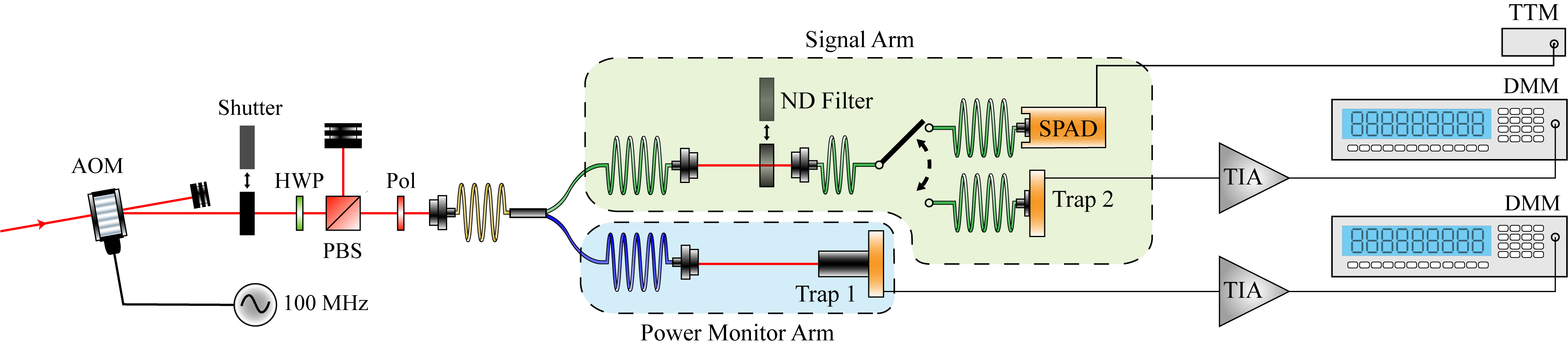
Figure 6: The experimental setup for detector calibration. Light at 780 nm is sent through an acousto-optic modulator (AOM) and a laser shutter, and then a system for power control consisting of a half-waveplate (HWP), a polarizing beam splitter (PBS), and a polarizer (Pol) on a motorized rotation mount. The light is then coupled into a $1\times 2$ fiber splitter whose outputs are the power monitor arm (blue) and the signal arm (green). The power monitor beam is free-space-coupled to a trap detector, Trap 1. The signal arm light may be sent through a calibrated ND filter on a motorized flip mount, and then it is coupled into another fiber which may be coupled to a second trap detector, Trap 2, or to the SPAD under test. Both trap detectors are attached to calibrated high-gain transimpedance amplifiers (TIAs) whose output voltages are read by 8-1/2-digit digital multimeters (DMMs), while the SPAD signals are sent to a time tagger module (TTM). The DMMs and TTM send data to a computer for processing. For the calibration measurements presented in this work, the AOM is always on, and both arms of the fiber splitter are used; for the reconstruction measurements, the AOM is used as an optical switch to produce pulses, and the power monitor arm is not used, reducing the setup to the one shown in Fig. 1 of the main text.

To measure the inputs to our reconstruction algorithm, we developed the experimental setup shown in Fig. 6, which allows us to measure everything we need with minimal reconfiguration. We use 780 nm light generated by a commercial external cavity diode laser. The beam passes through an acousto-optic modulator (AOM) (which is always on for the measurements of this section but is used to shape pulses for the reconstruction measurements presented in the main text), as well as a laser shutter. The light is passed through a set of polarization optics for power control: a half-waveplate and polarizing beamsplitter followed by a polarizer on a motorized rotation mount. This light is coupled into a $1\times 2$ fiber splitter which splits the light into a power monitoring arm and a signal arm. The power monitor arm is free-space-coupled to a Gentec TRAP7-Si-C-BNC [10] trap detector [11]. The signal arm contains a calibrated neutral density (ND) filter with transmittance $T_{\text{ND}}=0.001412(1)$ mounted on a motorized flip mount. After this filter, the light is coupled into a fiber whose other end may be coupled either to a second trap detector or to a SPAD to be tested. Both traps are connected to high-precision transimpedance amplifiers (Gentec SDX-1226-1) with gains set to $10^{8}$ V/A for all experiments here, and the resulting voltages are measured by two Keysight 3458A voltmeters. The SPADs that we calibrate and test in this work, two Excelitas SPCM-780-13-FC modules, are connected to an eight-channel Roithner TTM8000 time tagger, which receives SPAD clicks and sends data about the channel and time of the events to a computer for processing.

To calibrate our detectors, measuring some of the necessary quantities requires having first measured others, so we gather three types of data and analyze them in this order: (i) clicks from the SPAD with no signal light, to measure the background count rate, afterpulsing probability, and afterpulsing profile; (ii) clicks from the SPAD due to cw input light at various (uncalibrated) input rates, to gather information about recovery time effects; and (iii) clicks from the SPAD due to calibrated cw input light, to be compared with readings from the power monitor trap detector, to determine the detector efficiency.

Background Count Rate.

First, we analyze background count data. We take care to set up the environment exactly as it will be for reconstruction, including coupling the same fiber to the SPAD that will be used for reconstruction; we simply block all signal light. Then we collect time-tagged SPAD data for 12 hours to generate adequate statistics. We create full second-order correlation histograms, and fit to the linear background using the data corresponding to delays greater than 100 $\mu$s. This line can be written as $r^{2}\Delta t(t_{0}-t)$, where $\Delta t$ is the bin size and $t_{0}$ is the data collection time. The extracted $r_{b}$ is the background count rate. (Although this extracted count rate is affected by dead time losses, our background count rates are so low that the error due to this effect is negligible.)

An alternative strategy to measure the background count rate would be to simply count the total number of clicks in a dataset like the above (taken over a long time, with no input signal) and divide by the data collection time. This number will need to be corrected for the total afterpulsing probability, i.e. the probability for the detector to afterpulse at all times; however, to find this, we use a methodology (discussed in the next paragraph) that requires knowledge of the background count rate. Our method removes this circularity problem by eliminating the afterpulsing effects altogether while not being much more complicated.

Afterpulsing Profile and Probability, and Recovery Time.

After extracting this count rate, we also use the background counts dataset to generate a full afterpulsing profile. We form a first-and-second histogram from that data, which accurately maps the profile of afterpulsing clicks. In a first-and-second histogram, the background counts contribute an additional exponential factor $e^{-r_{b}t}$. Since the count rate is very low, the first-and-second data extends to several tens of milliseconds, so we can perform a fit beginning at 100 $\mu$s delay. We fit to an exponential with the known background rate but amplitude to be fitted, then extrapolate the fit to zero time delay and subtract it from the histogram to obtain the afterpulsing profile. (We manually set the bins corresponding to the recovery time to zero.) The profile obtained this way is the one shown in Fig. 4 above. If the histogram is then normalized by dividing by the total number of clicks in the dataset, then summing the remaining profile will give the probability of afterpulsing. Summing over the full profile gives the values in Table I of the main text.

We note that, purely due to statistical noise, the afterpulsing profile after the subtraction contains bins with slightly negative counts. However, because the calculation of $p_{a}$ in Eqn. 11 involves cumulative probabilities over the profile, we will never actually have negative numbers in the calculation. In some sense the integration in Eqn. 11 performs an average over these long times that mitigates the effects of the negative bins. These bins should not be set to zero; doing so would bias the resulting probabilities.

From the first-and-second histogram, we also identify the recovery time, defined to be the time of the first nonzero bin of the first-and-second histogram [8].

Dead and Reset Times.

To measure afterpulsing and recovery time effects, we use the DEP, which contains both afterpulsing and twilight counts, the latter being delayed until after the end of the recovery time [4]. Although these two phenomena are overlapped in time, we have a way to tell them apart due to their physical origins: afterpulsing originates with the detector circuitry, while twilight counts originate from real photons whose clicks simply got delayed. Thus by varying the rate of input photons, we vary the number of twilight counts, while the fraction of afterpulsing stays constant (for input photon rates that are not too high).

Based on this, our procedure is as follows [12]. For several different input count rates, which do not need to be known independently, we take cw click data with the SPAD under test. From these data we generate a first-and-sixth histogram to measure the count rate as discussed above. We then generate a first-and-second histogram from the same dataset, and use this to extract the probability of a DEP click. Considering afterpulsing in more detail, let us suppose it has a temporal profile $a(t)$. At low count rates, this is the entire DEP. Then, after the recovery time ends, afterpulsing is competing with the Poissonian process of clicks from input photons, which leads to the second click having a probability density function

$$p(t)=(1-\bar{p}_{a})re^{-r(t-\tau_{r})}+\bar{p}_{a}\left[p_{a}(t)e^{-r(t-\tau_{r})}+(1-P_{a}(t))re^{-r(t-\tau_{r})}\right],\hskip 5.0ptt\geq\tau_{r}.$$ (20)

Here as before, we define the recovery time $\tau_{r}$, and we defined the magnitude $\bar{p}_{a}=\int_{0}^{\infty}a(t)\,dt$, the probability $p_{a}(t)=a(t)/\bar{p}_{a}$, and the cumulative probability $P_{a}(t)=\int_{0}^{t}p_{a}(t^{\prime})\,dt^{\prime}$. At long times, $p_{a}(t)\rightarrow 0$ and $1-P_{a}(t)\rightarrow 0$, so only the first term is non-negligible. We use this as a background function for subtraction, multiplied by $N\Delta t$ to convert it to a number of events per bin. To handle the recovery time region, we find all negative bins preceding the maximum of the subtracted histogram and add back the subtracted function, which sets bins that had zero clicks to zero, and treats all clicks in this region as legitimate clicks to be included in the counting.

What remains in Eqn. 20 after the subtraction consists of two terms. The second of those terms, in which afterpulsing is interrupted by a count from a photon, is negligible for all count rates discussed here. We can see this heuristically as follows. Let us model afterpulsing as an exponential decay, $p_{a}(t)\approx e^{-t/t_{a}}/t_{a}$. Then $P_{a}(t)=1-e^{-t/t_{a}}$. Then the first term is larger than the second by a factor $1/(rt_{a})$. Fig. 4 suggests our detectors have an effective exponential decay timescale of just a few ns; thus, for the largest count rates in our measurements, $1/(rt_{a})\sim 10$. Therefore we can safely neglect the last term in Eqn. 20. Thus, after the subtraction, we are left with the second term of Eqn. 20. Dividing the subtracted profile by $e^{-r(t-\tau_{r})}$, we obtain $\bar{p}_{a}p_{a}(t)$. This is summed from zero delay to twice the recovery time, which should capture all twilight counting effects while reducing uncertainty from the subtraction process. Dividing this sum by the number of clicks in the dataset, we finally obtain the fraction of clicks in the DEP.

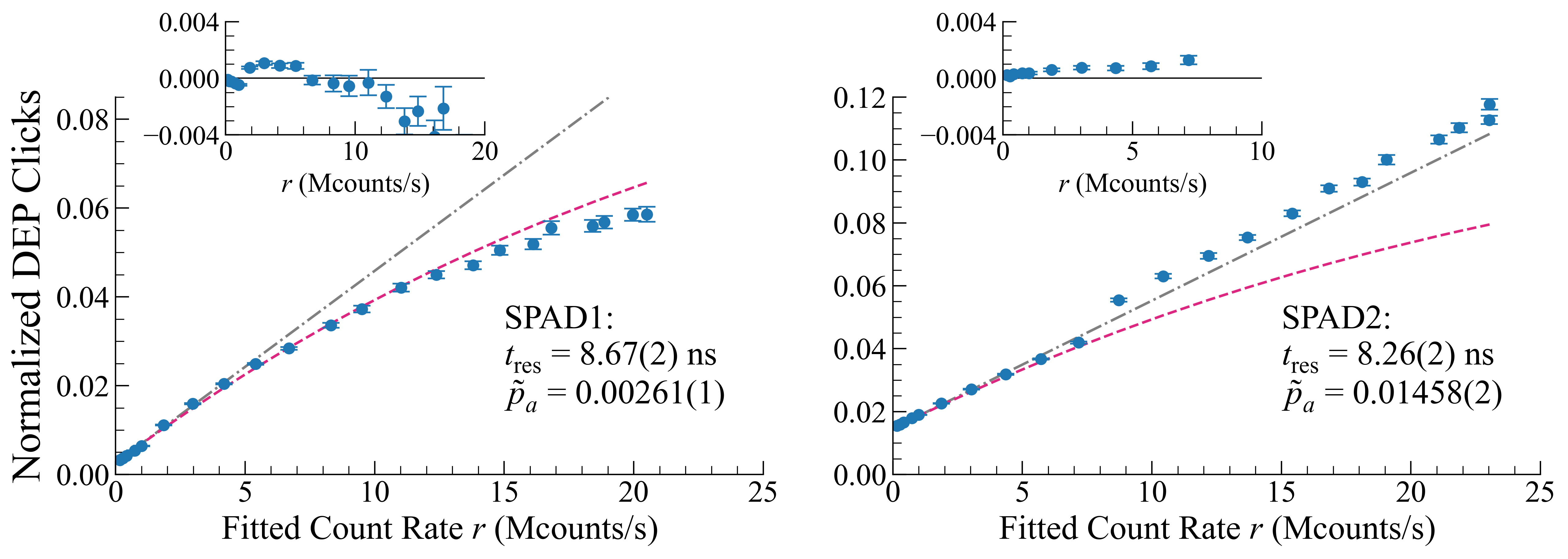
Figure 7: Normalized DEP clicks as a function of count rate obtained from first-and-sixth histograms, for SPAD1 (left) and SPAD2 (right). The data (blue dots) are shown with error bars representing two standard deviations. As discussed in the text, the previously measured afterpulsing probability is used as the y-intercept of a linear fit to the data points with count rates below 5 Mcounts/s, which yields a value of the reset time $t_{\text{res}}$. The gray dash-dotted line shows this linear fit extrapolated over the plot. The dashed magenta line is the more accurate Eqn. 21, using the previously obtained values of $p_{a}$, $t_{\text{res}}$, $t_{\text{rec}}$. As discussed in the text, as the count rate increases, the DEP clicks deviate from this model, and the two detectors deviate in different ways. Insets show residuals between the data points and the magenta model line, again with two-standard-deviation error bars.

Using this procedure for several input count rates from about $2\times 10^{5}$ to over $2\times 10^{7}$ counts/s, we obtain the data shown in Fig. 7. At low count rates (below about 5 Mcounts/s), we observe linear behavior, but at high count rates, a deviation from linearity becomes apparent. We model the DEP as occurring immediately after the end of the reset time and being composed of two types of clicks: (i) afterpulsing with probability $p_{a}$, and (ii) twilight counts, with probability that is the product of a photon arriving and the detector sensing it. The probability of a single photon arriving in the recovery time and being detected is

$$p_{1}=\int_{t_{d}}^{t_{\text{rec}}}re^{-rt_{\text{rec}}}\frac{t-t_{d}}{t_{\text{rec}}-t_{d}}\,dt=\frac{1}{2}re^{-rt_{\text{rec}}}(t_{\text{rec}}-t_{d}),$$

where the function $(t-t_{d})/(t_{\text{rec}}-t_{d})$ describes the quantum efficiency model adopted in Fig. 1. So we can write the total DEP probability as

$$p_{\text{DEP}}=p_{a}+\frac{1}{2}(1-p_{a})re^{-rt_{\text{rec}}}(t_{\text{rec}}-t_{d}),$$ (21)

where the second term comes from the integral $p_{1}$. When $rt_{\text{rec}}\ll 1$, this reduces to a linear function, $\tilde{p}_{\text{DEP}}=p_{a}+(1/2)(1-p_{a})r(t_{\text{rec}}-t_{d})$, in which the offset is the afterpulsing probability and the slope is related to the reset time. But as the count rate increases, the saturation described by the exponential $e^{-rt_{\text{rec}}}$ becomes apparent. Note that one can generalize the above expression for $p_{1}$ to calculate additional terms for the probability of two or more photons arriving and at least one being detected. In Fig. 7, the magenta dashed lines include terms with two photons arriving during the recovery time. We perform a linear fit using the data points with count rates below 5 Mcounts/s, with the fit offset constrained using the afterpulsing probability found previously, so only the linear coefficient is a fit parameter. (This constraint produces no inconsistency since the afterpulsing probability was also found with a first-and-second histogram as described above.) This fit yields the reset time. The final values for the afterpulse probability (within two recovery times) and the reset time for both SPADs under test are given in Fig. 7. Note also that, from the reset time and the recovery time, we can determine the dead time as $t_{\text{dead}}=t_{\text{rec}}-t_{\text{reset}}$.

The deviations from Eqn. 21 in the data may be attributed to a number of possible mechanisms, such as changing dead, reset, or recovery times, or non-Markovianity which changes the effective afterpulsing probability (both of which were discussed in subsection A.V. above). These deviations are not modeled by our algorithm, but in any case, they do not appear to be the primary limitation of the algorithm at high count rates.

Quantum Efficiency.

Finally, it remains to measure the detector efficiency. To measure the DE, we need to compare a known input photon rate to a count rate measured by the SPAD, and the measured count rate needs to be the count rate the SPAD would measure if there were no recovery time effects, so that the measured detector efficiency is that of a fully armed detector, as required by our model. Typically the independent measurement is done with a conventional photodiode, and there is a gap of several orders of magnitude between what the photodiode can measure reliably and what the SPAD can accept. We decrease this gap from both sides. On one end, our photodiodes are trap detectors [11] with high-gain and high-precision readout electronics that allow us to sense 100 pW reliably (the system’s noise-equivalent power over a measurement of 300 s is roughly 1 pW). On the other end, as previously shown, extracting count rates using first-and-$n$ histograms allows us to reliably extract count rates up to tens of millions of counts per second, which is higher than conventional methods can achieve without correction for dead time effects. These two techniques reduce the gap between the needed powers to just 2 to 3 orders of magnitude, which can be bridged by commercial ND filters.

The input power is measured in the power monitor arm of the setup in Fig. 6. The optical power is free-space-coupled to a trap detector with efficiency $\eta_{\text{pm}}$, which converts the power to a current with a responsivity $R$; this current is converted to a voltage by a transimpedance amplifier (TIA) with gain $G$, and this voltage $V_{\text{meas}}$ is read by an 8-1/2-digit voltmeter. Thus the power in the power monitor arm is calculated as $P_{\text{pm}}=V_{\text{meas}}/(\eta_{\text{pm}}RG)$. Then, by coupling the signal arm into a fiber coupled to a second trap detector, we independently measure both the transmittance of the ND filter $T_{\text{ND}}$ and the power ratio $R_{\text{AB}}$ between the power monitor and signal branches. The ND filter is then placed in the signal path for the measurements of the detector efficiency. As a result, the power into the SPAD under test is $P_{in}=P_{\text{pm}}R_{\text{AB}}T_{\text{ND}}$.

Finally, we compare this input power to a count rate extracted from a first-and-sixth histogram as described above. The measured count rate must be corrected for background counts, so the rate to compare to is just $\mathcal{R}=\mathcal{R}_{\text{meas}}-\mathcal{R}_{\text{dc}}$, where $\mathcal{R}_{\text{dc}}$ is the independently measured background count rate.

Putting everything together, the detector efficiency is

$$\eta=\frac{\mathcal{R}\frac{hc}{\lambda}}{P_{in}}=\frac{\mathcal{R}_{\text{meas}}-\mathcal{R}_{\text{dc}}}{V_{\text{meas}}R_{\text{AB}}T_{\text{ND}}/\eta_{\text{pm}}RG}\frac{hc}{\lambda}.$$ (22)

For all of the measurements here, $\lambda=780$ nm with a linewidth of at most 1 MHz and a drift of not more than about 50 MHz, limited by a laser lock to a commercial wavemeter. In addition, $R=0.6293$ A/W is the responsivity calculated using a simple one-photon-equals-one-electron rule, and $G=10^{8}$ V/A for all the measurements here.

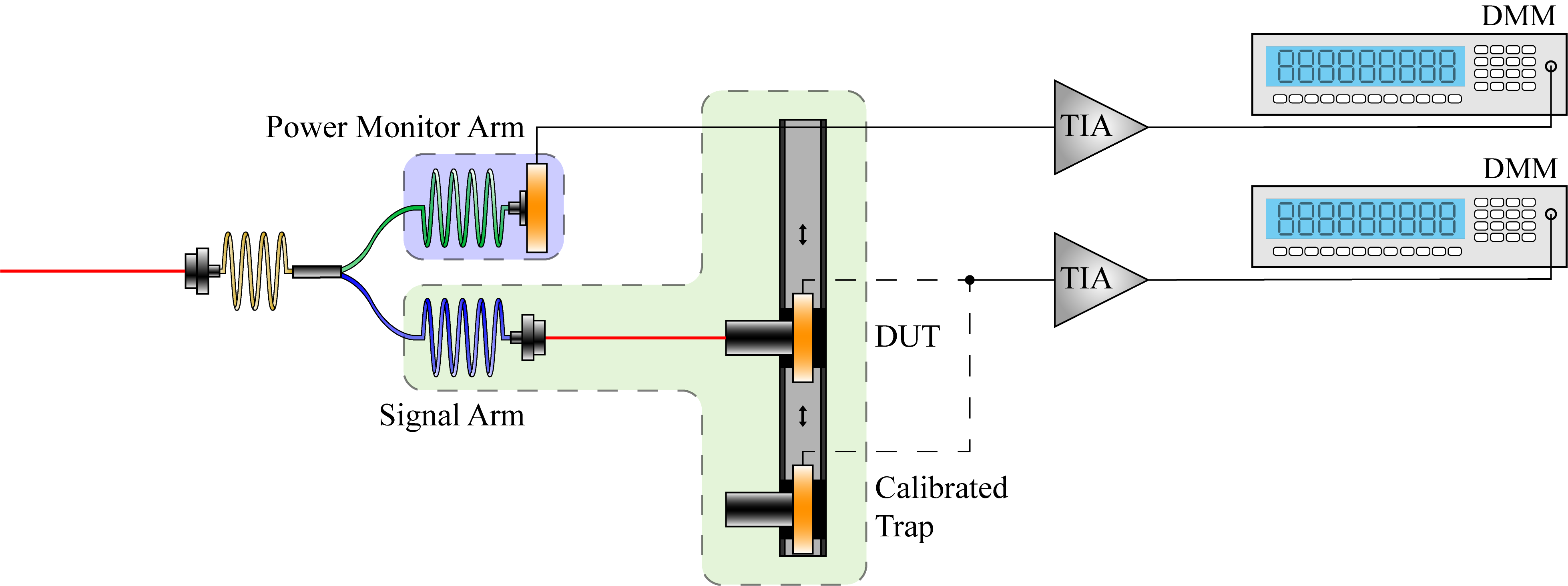
Figure 8: The setup used to transfer calibration to the trap detectors used in our measurements. Input light is sent through a fiber splitter into two arms, a power monitor arm and a signal arm. The former is coupled directly by fiber into a trap detector whose efficiency is not necessary to the calculations. The signal arm light is coupled into a fixed free-space path. The calibrated trap and the device under test (DUT) are transferred into and out of this path via a 1D optical rail. All traps are connected to high-gain TIAs which are connected to high-precision voltmeters.

To measure our trap detector’s efficiency $\eta_{\text{pm}}$, we use a trap detector previously calibrated at the Visible to Near-Infrared Spectral Comparator Facility of the National Institute of Standards and Technology (NIST) [13]. We transfer the calibration of this trap to our traps using the relatively simple setup shown in Fig. 8. Light is split by a fiber splitter into two paths, a power monitor path and a signal path. The power monitor path is directly fiber-coupled into a trap detector whose efficiency is not necessary to know. The signal path light is coupled to a fixed free-space path; the NIST-calibrated detector and the device under test are alternately slid into this path using optical rails. First, we take 3 hours of continuous measurements of the voltages and compute an Allan deviation. From this, we set the duration of an individual measurement as 200 seconds. Then we perform 30 measurement cycles, over two days. Each measurement cycle consists of a period of 200 s of collecting voltage data from the NIST-calibrated detector and the power monitor trap, followed by sliding the device under test into the signal beam path and taking another period of 200 s of readings from the device under test and the power monitor traps. Thus each cycle gives a total of four sets of readings: the signal path readings with the NIST-calibrated trap $\{V_{\text{i,sg,cal}}\}$, the power monitor readings taken at the same time $\{V_{\text{i,pm,cal}}\}$, the signal path readings with the device under test $\{V_{\text{i,sg,DUT}}\}$, and the power monitor readings taken at the same time $\{V_{\text{i,pm,DUT}}\}$, with $i\in[1,N]$ indexing the $N$ readings in each set. In this way, for one measurement cycle, we calculate

$$\frac{\eta_{\text{pm}}}{\eta_{\text{cal}}}=\frac{1}{N}\sum_{i=1}^{N}\frac{\tilde{V}_{\text{i,sg,DUT}}/\tilde{V}_{\text{i,pm,DUT}}}{\tilde{V}_{\text{i,sg,cal}}/\tilde{V}_{\text{i,pm,cal}}}$$ (23)

where $\tilde{V}$ denotes the background-subtracted versions of the sets $V$, and $\eta_{\text{cal}}$ is the efficiency of the NIST-calibrated trap detector.

The quantities $T_{\text{ND}}$ and $R_{\text{AB}}$ also require separate measurement, but the measurement principles are similar to the measurement of $\eta_{\text{trap}}$. To calibrate the ND filter, we follow a technique similar to Ref. [14] (which also inspired the measurement of $\eta_{\text{pm}}$ just described). Using the setup in Fig. 6, the signal arm’s fiber is attached to a trap detector, and readings from the signal and monitor arms’ voltmeters are taken and compared. We compare 300 sec of readings with the filter in to 300 sec of readings with the filter out, so one measurement cycle gives four sets of readings: the signal path readings with the filter in $\{V_{\text{i,sg,in}}\}$, the power monitor readings taken at the same time $\{V_{\text{i,pm,in}}\}$, the signal path readings with the filter out $\{V_{\text{i,sg,out}}\}$, and the power monitor readings taken at the same time $\{V_{\text{i,pm,out}}\}$, with $i\in[1,N]$ indexing the $N$ readings in each set. The final calculation of the ND filter transmittance is then calculated as the mean

$$T_{\text{ND}}=\frac{1}{N}\sum_{i=1}^{N}\frac{\tilde{V}_{i,\text{sg,in}}/\tilde{V}_{i,\text{pm,in}}}{\tilde{V}_{i,\text{sg,out}}/\tilde{V}_{i,\text{pm,out}}},$$ (24)

where $\tilde{V}$ denotes the background-subtracted versions of the sets $V$. The results of 24 hr of measurements are shown in Fig. 9a. We obtained the final value $T_{\text{ND}}=0.001412(1)$. A discussion of uncertainties is reserved for the next section.

The measurement of the ratio of power in the two branches $R_{\text{AB}}$ is performed somewhat similarly, except that there are not two independent measurements needed: we simply take voltage readings for 300 seconds, and then divide the background-subtracted readings element-wise to obtain the ratio. Mathematically,

$$R_{\text{AB}}=\frac{1}{N}\sum_{i=1}^{N}\frac{V_{i,\text{sg}}}{V_{i,\text{pm}}}$$ (25)

where the notation is similar to the last paragraphs. Note that, in the signal arm, the trap is fiber-coupled, so that $R_{\text{AB}}$ includes the fiber coupling in addition to other factors such as the imbalance of the fiber splitter. Through a 24-hr measurement we obtained $R_{\text{AB}}=61.5(1)\leavevmode\nobreak\ \%$.

The dark current of the traps was measured using a similar methodology to the above. We blocked all of the light and then took 12 hr of readings from the traps and performed an Allan deviation. This determines the time over which to measure and average the dark current, which was also 300 seconds. This measurement must be done for each setting of the TIA gain used. For a gain of $10^{8}$ V/A, the dark currents in both traps were measured to be $\approx 10^{-4}$ V.

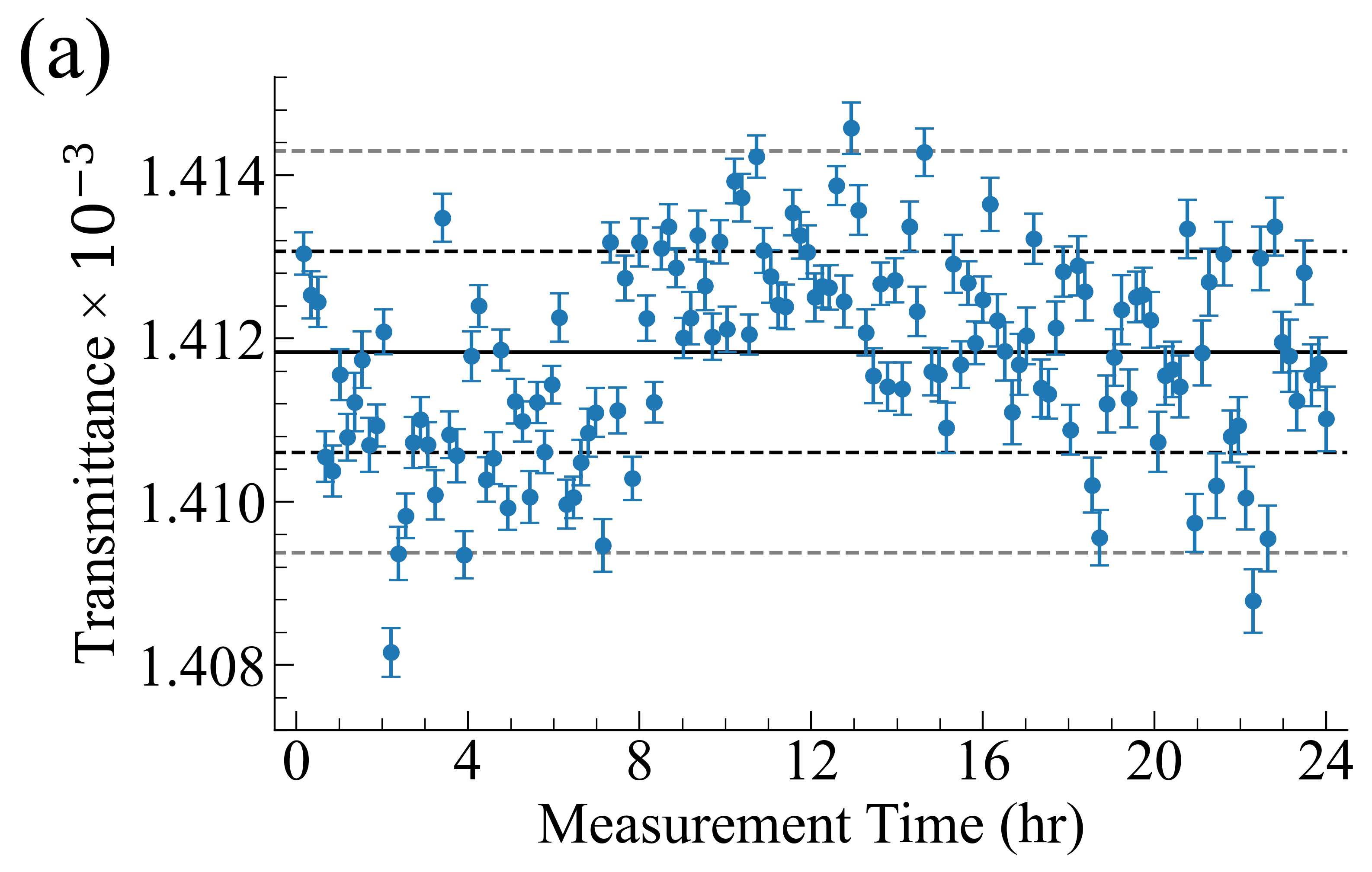
(a)

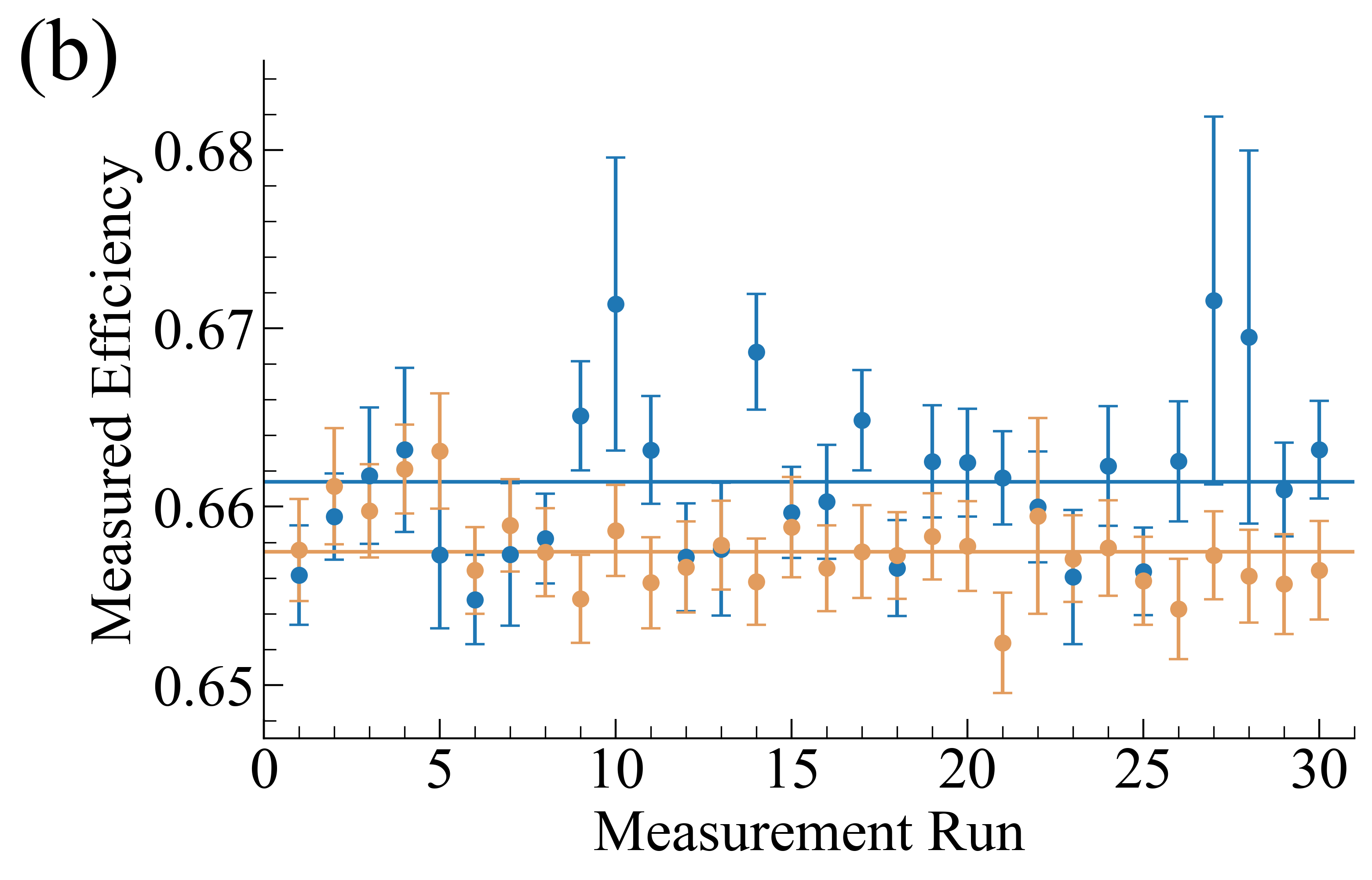
(b)

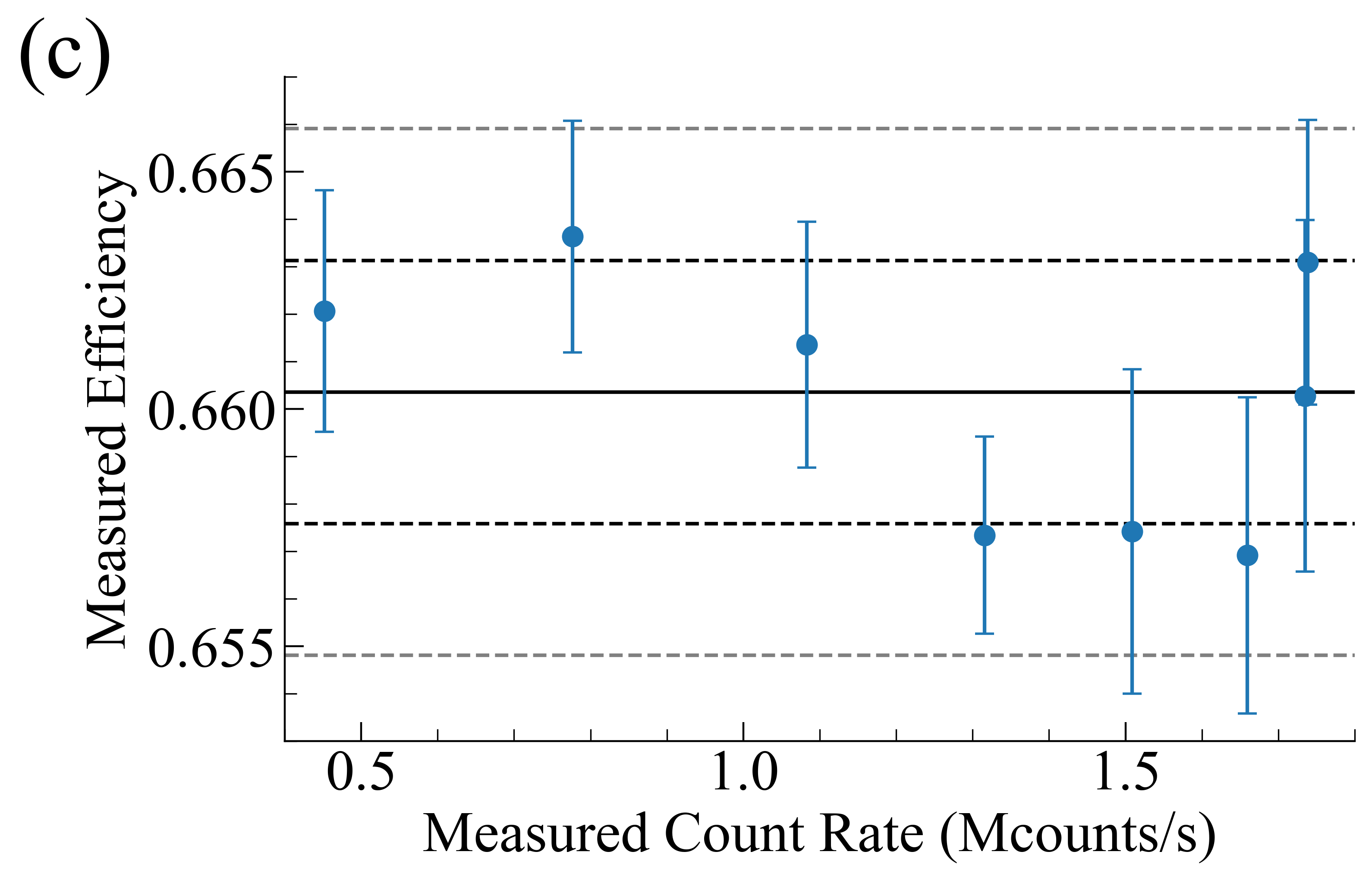
(c)

Figure 9: Detector efficiency measurement data. (a) Measured transmittance of the ND filter from 140 runs over 24 hours, with result $T_{\text{ND}}=0.001412(1)$. Error bars represent one standard deviation uncertainty. The solid black line indicates the mean, and the dashed lines indicate one (black) and two (gray) standard deviations of the data. We attribute the variation to environmental changes over the course of the 24 hr measurement. (b) Two sets of 30 measurements of the detector efficiency of SPAD2, taken at two different input powers. Error bars represent one standard deviation uncertainty. The somewhat large variation is due primarily to a small number of voltage readings accompanying each measurement (as few as eight). Horizontal lines show the corresponding means of each data set. (c) Average detector efficiency measurements at several input count rates for SPAD2. Error bars represent one standard deviation uncertainty. The count rates on the horizontal axis are extracted using first-and-fourth histograms of the data. The solid black line indicates the mean, and the dashed lines indicate one (black) and two (gray) standard deviations of the data. We attribute most of the variation to environmental changes over the course of the 24 hr measurement.

Having performed measurements of all of the necessary quantities, we then measured the detector efficiency. We chose eight input powers ranging from detected count rates of $2\times 10^{5}$ counts/s to $2\times 10^{6}$ counts/s, and for each rate we took 30 measurements of $\eta$. A measurement cycle consists of opening a shutter to expose both the SPAD and the power monitor trap to the laser power for varied amounts of time between 4 s and 40 s, with the highest count rates using the shortest times and vice versa. We then match up the power monitor readings to the SPAD time tags from each cycle to obtain values of $\eta$ for each run using Eqn. 22. Two sets of 30 measurement runs at two different input powers are shown in Fig. 9b. All 30 measurements were then averaged to obtain a measurement of $\eta$ at each count rate. These average values are shown plotted against count rate in Fig. 9c. Since these did not show significant variation over the count rates used here, we averaged all of these measurements to obtain a final value for $\eta$ for each detector under test. The results are given in Table I of the main text.

B.III Calibration of Input Coherent States

To validate our reconstruction technique, we need to compare the reconstruction to an independently measured distribution, so we separately calibrated the coherent states we used for reconstruction. Fig. 6 shows the experimental setup we used for this purpose; before coupling the signal fiber into the SPAD for reconstruction measurements, we coupled it into Trap 2, with efficiency $\eta_{\text{trap}}$ measured similarly to $\eta_{\text{pm}}$ above. We took voltmeter readings from Trap 2 with no ND filter in the path. The power onto Trap 2 is calculated as $P_{\text{in}}=V_{\text{meas}}/(\eta_{\text{trap}}RG)$, with notation similar to previous sections. For the reconstruction measurement, the signal arm fiber is coupled into the SPAD and the calibrated ND filter is then inserted to deliver power $T_{\text{ND}}P_{\text{in}}$ to the SPAD. The power monitor arm was not used for this measurement.

A final factor to consider in this calibration is that the measurement of $P_{\text{in}}$ is done with continuous-wave (cw) light, so we need to multiply the power by a factor that tells us the total average energy in a pulse. The shape of the pulse as well as the peak power delivered during data collection must be taken into account by this factor. (The latter can be different from the cw power, for instance due to AOM thermalization effects.) We measure this factor directly using the SPADs. We take $2\times 10^{6}$ experimental cycles of each of two situations: (i) the AOM fully on and thermalized, and (ii) the AOM set to modulate its drive as appropriate to provide the pulse we wish to analyze. For these data we attenuate the beam using the polarizer after the AOM but before the detector, so that the count rate into the SPAD is low enough to be unaffected by recovery time effects while still probing the AOM behavior accurately. We subtract a background from both the pulsed and cw datasets, then choose a window of time of duration $T$ (equal to the duration used for the number state reconstruction analysis) and divide the total number of clicks in the pulsed dataset in this window by the total number in the cw dataset in the same window. We denote this “shape factor” $f_{s}$.

Putting all of this together, we calculate the expected number of photons in any given coherent pulse as (Eqn. 5 of the main text)

$$\bar{n}_{\text{exp}}=\frac{P_{\text{in}}f_{s}}{hc/\lambda}=\frac{V_{\text{meas}}T_{\text{ND}}f_{s}}{\eta_{\text{trap}}RG}\frac{1}{hc/\lambda}.$$ (26)

B.IV Effects of Detection System Timing

The SPADs that we calibrate and test in this work, two Excelitas SPCM-780-13-FC modules, are connected to an eight-channel Roithner TTM8000 time tagger module (TTM).

The SPADs have timing jitter of 350 ps. However, our algorithm does not depend on the timing of any particular click, except in estimating the photon profile $\gamma(t)$. For this, a large number of experimental cycles allows us to average over detector jitter, giving a good estimation of $\gamma(t)$.

The TTM has an effective resolution of about 164 ps. Because we use bins of about 1 ns width (6 TTM bins), we believe the TTM resolution does not limit our results in any way.

C Discussions of Uncertainties

In this section we discuss the calculation of all uncertainties presented in the paper.

C.I Uncertainties in Detector Characterization

The first quantity we measure in detector characterization is the background count rate. This is estimated using the data from a full second-order correlation histogram after 100 $\mu$s. To estimate the uncertainty, we bootstrap off of the fitted number of clicks in each bin, re-fitting the count rate each time; the standard deviation of these fitted count rates gives an estimate of the uncertainty in the background count rate.

Next, the afterpulsing probability is determined by applying this background count rate to a first-and-second histogram of dark count data, subtracting, and summing what remains. We estimate the uncertainty in the afterpulsing probability by using the previously estimated dark count rate uncertainty and the uncertainty in the fit amplitude to bootstrap random background profiles, which are subtracted. The standard deviation of the resulting set of afterpulsing probabilities is our estimate of the uncertainty in the afterpulsing probability. In this process we sum the background-subtracted profile only to the first two recovery times, which reduces sensitivity to the fitted amplitude; thus we obtain the probability $p_{a,0}$ of afterpulsing within two recovery times, and the uncertainty $u_{a,0}$ in that quantity. To estimate the uncertainty on the probability of afterpulsing over any time window, we fractionally scale $u_{a,0}$. That is, if the probability of afterpulsing in a time window from $t=0$ to $t=t_{0}$ is $p_{a}(t_{0})$, we calculate the uncertainty as $u_{a}(t_{0})=u_{a,0}p_{a}(t_{0})/p_{a,0}$.

The recovery time is estimated by multiplying the bin size by the number of bins with zero events at the start of a second-order histogram. A simple way to estimate the uncertainty is to thus use half a bin size. In our case $\Delta t=164.6$ ps, the limit of our time tagger resolution according to the device specifications. Because we have many of these histograms at many different count rates, we can take an average over the measured recovery times, and divide the half-bin-width uncertainty by the square root of the number of histograms analyzed to reduce the estimated uncertainty.

The reset time is obtained by a linear fit to the fraction of clicks in the DEPs of first-and-second histograms at different count rates, as shown in Fig. 7. Each of the points in this fitting procedure has an uncertainty, which we estimate by combining in quadrature two uncertainty sources: (1) the total number of clicks in the peak (whose uncertainty we take to be the square root), and (2) the uncertainty in the slope of the linear background subtracted from the histogram to obtain the DEP. To estimate the latter, we perform a simple bootstrapping procedure on the data. Then we perform the subtraction-and-summation process discussed above in Monte Carlo fashion, randomly sampling count rates from a Gaussian whose mean is the fitted count rate and whose uncertainty is the bootstrapped uncertainty. The standard deviation of the resulting set of counts in the DEP gives an estimate of the uncertainty in that number due to the uncertainty in the slope of the subtracted background. We sum (1) and (2) in quadrature to obtain the uncertainty in the fraction of clicks in the DEP. After fitting the data to a line using these estimated uncertainties as weights, we constrain the reduced $\chi^{2}$ to unity and use the resulting factor to scale the fitted parameter uncertainties. These are the final results we present in Table I of the main text and in Fig. 7. We note also that we compute the dead time simply as $t_{\text{dead}}=t_{\text{rec}}-t_{\text{reset}}$, so the uncertainty in the dead time is propagated from the uncertainties in the recovery and reset times.

Table 2: Summary of sources of uncertainty for the detector efficiency as calculated in Eqn. 27. From left to right, columns are: quantity that contributes to the uncertainty in $\eta$, and its value; form of that quantity’s contribution to $d\eta/\eta$, and the value of that contribution as a percentage of $\eta$; and a brief explanation of that source of uncertainty. Some of the numerical values given are typical values from a single measurement run, as appropriate. In the last row we give the calculated value and uncertainty for the DE using the values of this particular measurement run. These values come from a run measuring the DE of SPAD2, whose final measured DE is $\eta=0.660(3)$, with a fractional uncertainty (one standard deviation) of 0.45 %. (Note that the value in the final row of the table is the value of $\eta$ obtained for this particular run, so it differs slightly from the final averaged value just given.) In the last column, (W)SD stands for (weighted) standard deviation.

Measurand		Contribution to $\delta\eta/\eta$ (%)		Source of Uncertainty
$\mathcal{R}_{\text{dc}}$	203(1) counts/s	$\delta\mathcal{R}_{\text{dc}}/(\mathcal{R}_{\text{meas}}-\mathcal{R}_{\text{dc}})$	$7\times 10^{-5}$	Fit to second-order histogram
$\mathcal{R}_{\text{meas}}$	1.512(2) Mcounts/s	$\delta\mathcal{R}_{\text{meas}}/(\mathcal{R}_{\text{meas}}-\mathcal{R}_{\text{dc}})$	0.13	Fit to first-and-fourth histogram
$V_{\text{meas}}$	41.96(9) mV	$\delta V_{\text{meas}}/V_{\text{meas}}$	0.22	SD of the mean of points
$R_{\text{AB}}$	0.615(1)	$\delta R_{\text{AB}}/R_{\text{AB}}$	0.16	WSD of 140 points over 24 hr
$T_{\text{ND}}$	0.001412(1)	$\delta T_{\text{ND}}/T_{\text{ND}}$	0.09	WSD of 140 points over 24 hr
$\eta_{\text{trap}}$	0.994(3)	$\delta\eta_{\text{trap}}/\eta_{\text{trap}}$	0.29	WSD of 30 points over two days
$\eta$	0.661(3)	—	0.43	—

^a Typical value for one measurement cycle

Finally we discuss the uncertainty in the detector efficiency. The sources of uncertainty are summarized in Table 2 with values for one measurement of the DE of SPAD2. Recall that we compute the detector efficiency as

$$\eta=\frac{\mathcal{R}\frac{hc}{\lambda}}{P_{in}}=\frac{\mathcal{R}_{\text{meas}}-\mathcal{R}_{\text{dc}}}{V_{\text{meas}}R_{\text{AB}}T_{\text{ND}}/\eta_{\text{trap}}RG}\frac{hc}{\lambda}.$$ (27)

The final value for $\eta$ and its uncertainty for each detector is a weighted average and standard deviation, respectively, of the values for $\eta$ at several powers, as shown in Fig. 9c. Each of these and its uncertainty are in turn the weighted average and standard deviation of 30 individual measurements of $\eta$ at a given input power (two sets of 30 at two input powers are shown in Fig. 9b). For each individual run, we calculate the uncertainty in $\eta$ using standard error propagation techniques:

$$\left(\frac{\delta\eta}{\eta}\right)^{2}=\frac{\delta\mathcal{R}_{\text{meas}}^{2}+\delta\mathcal{R}_{\text{dc}}^{2}}{\left(\mathcal{R}_{\text{meas}}-\mathcal{R}_{\text{dc}}\right)^{2}}+\left(\frac{\delta V_{\text{meas}}}{V_{\text{meas}}}\right)^{2}+\left(\frac{\delta R_{\text{AB}}}{R_{\text{AB}}}\right)^{2}+\left(\frac{\delta T_{\text{ND}}}{T_{\text{ND}}}\right)^{2}+\left(\frac{\delta\eta_{\text{trap}}}{\eta_{\text{trap}}}\right)^{2}.$$ (28)

We discuss the nature of the uncertainties in each quantity below, with typical values and contributions to the final uncertainty given in Table 2.

First, the uncertainty in the dark count rate $\delta\mathcal{R}_{\text{dc}}$ is found by bootstrapping uncertainties on the fit to a full second-order correlation histogram of dark count data, as previously discussed. Similarly, the uncertainty in the measured click rate $\mathcal{R}_{\text{meas}}$ is found by bootstrapping uncertainties on the fit to the first-and-sixth histograms that yield $\mathcal{R}_{\text{meas}}$.

Next, $V_{\text{meas}}$ is the average of several background-subtracted readings of the voltmeter attached to the power monitor trap detector during the time the SPAD is collecting count rate data. We take the uncertainty in $V_{\text{meas}}$ to be the standard deviation of the individual readings, divided by the square root of the number of readings (which is supported by Allan variance curves indicating the Gaussian nature of the noise), summed in quadrature with the uncertainty in the independently-measured dark current. Because we only sample the voltmeter about 3 times per second (this is software-limited; the voltmeter’s integration time is 50 ms), and the shutter is sometimes open for as little as a few seconds, this can be the largest source of uncertainty for some of the measurement runs.

The uncertainties on $R_{\text{AB}}$, $T_{\text{ND}}$, and $\eta_{\text{trap}}$ are all estimated using similar methods. For $R_{\text{AB}}$ and $T_{\text{ND}}$, the values and uncertainties are taken to be the weighted average and standard deviation of 140 measurements each taken continuously over 24 hr, while for $\eta_{\text{trap}}$ there are 30 total measurements taken at various times over two days. We use the full standard deviation (as opposed to a standard deviation of the mean) because the measurement samples environmental variation that we wish to include in the uncertainty. Each individual measurement is in turn a simple standard deviation of the element-wise ratios used to compute the value of the quantity, the quantities in the sums of Eqs. 25, 24, and 23 respectively, divided by the square root of the number of readings in the cycle.

We note that it is possible to characterize the variations and uncertainties in an ND filter much more carefully than we did [14]. For this work we adopted a simplifying approach by only measuring the transmittance of the filter in situ. The filter was mounted on a motorized flip mount that allowed for precise replacement of the filter in the beam path, so that we always sampled the same location on the filter (as an alternative to measuring different locations on the filter and including the results in an uncertainty analysis). By measuring the filter over the course of one full day we believe we adequately sample the variation of the transmittance caused by temperature and humidity variations in the lab. We also believe the effects of detector nonlinearity and interference within the filter, which is absorptive, to be negligible. This means that not only do we neglect etaloning effects on the measured powers, but we also neglect any additional wavelength dependence of the transmittance due to these effects. Furthermore, the laser is sufficiently narrow, and its drifts are sufficiently small, that we can neglect all variations in transmittance as a function of wavelength.

For $\eta_{\text{trap}}$, the quantity we really measure is $\eta_{r}\equiv\eta_{\text{trap}}/\eta_{\text{cal}}$. The calibration itself has some uncertainty, so that we compute the overall uncertainty as

$$\left(\frac{\delta\eta_{\text{trap}}}{\eta_{\text{trap}}}\right)^{2}=\left(\frac{\delta\eta_{r}}{\eta_{r}}\right)^{2}+\left(\frac{\delta\eta_{\text{cal}}}{\eta_{\text{cal}}}\right)^{2}.$$ (29)

For us, $\eta_{\text{cal}}=0.989(3)$.

We suppose that the electronics—the TIA gain and the voltmeter—add negligible statistical uncertainty, but we mention the small systematic uncertainties here. The gain of the transimpedance amplifier has a quoted 0.025 % accuracy. We estimate the voltmeter to contribute a systematic uncertainty of no more than 0.01 %. We also suppose the wavelength of the light to have negligible uncertainty, and therefore no contribution to the uncertainty of the detector efficiency, either directly or through variations in $T_{\text{ND}}$ or $\eta_{\text{trap}}$ with wavelength.

C.II Uncertainties in Input Coherent State Calibration

Finally, we briefly discuss the uncertainty in the calibrated input coherent state average photon numbers $\bar{n}_{\text{exp}}$ of Eqn. 26 (or Eqn. 5 of the main text). The uncertainty is calculated as

$$\left(\frac{\delta\bar{n}_{\text{exp}}}{\bar{n}_{\text{exp}}}\right)^{2}=\left(\frac{\delta V_{\text{meas}}}{V_{\text{meas}}}\right)^{2}+\left(\frac{\delta T_{\text{ND}}}{T_{\text{ND}}}\right)^{2}+\left(\frac{\delta\eta_{\text{trap}}}{\eta_{\text{trap}}}\right)^{2}+\left(\frac{\delta f_{s}}{f_{s}}\right)^{2}.$$ (30)

We have discussed the nature of $\delta T_{\text{ND}}$ and $\delta\eta_{\text{trap}}$ already. Further, because $V_{\text{meas}}$ is simply the average of a set of voltage readings, we take $\delta V_{\text{meas}}$ to be the standard deviation of those readings, divided by the square root of the number of readings.

The shape factor $f_{s}$ is calculated as a ratio $\tilde{N}_{\text{pd}}/\tilde{N}_{\text{cw}}$ where $\tilde{N}_{\text{pd}}$ is the total number of clicks in the pulsed dataset and $\tilde{N}_{\text{cw}}$ that in the cw dataset, and the tildes denote background-subtracted quantities. The number of background clicks over the time window of interest is $N_{\text{bg}}$. We suppose the uncertainties in $N_{\text{pd}}$, $N_{\text{cw}}$, and $N_{\text{bg}}$ to be the square roots of the respective quantities, so standard uncertainty propagation gives

$$\left(\frac{\delta f_{s}}{f_{s}}\right)^{2}=\frac{N_{\text{pd}}}{\tilde{N}_{\text{pd}}^{2}}+\frac{N_{\text{cw}}}{\tilde{N}_{\text{cw}}^{2}}+\left(\frac{N_{\text{pd}}-N_{\text{cw}}}{\tilde{N}_{\text{pd}}\tilde{N}_{\text{cw}}}\right)^{2}N_{\text{bg}}.$$ (31)

C.III Uncertainties on Reconstructed Distributions

We obtain uncertainties on the reconstructed distributions by Monte Carlo sampling. There are two types of uncertainties involved. (1) Sampling uncertainties, in which the detected click distribution varies from $\mathbb{D}\mathbf{P}$ (using the notation from the beginning of Section A) due to the experiment being finite and probabilistic. This produces statistical uncertainties on the number components of the distribution. We estimate this uncertainty by assuming each number component of the measured distribution follows a Poissonian distribution, which, while not really correct, should produce a reasonable estimate of the magnitude of the effects. (2) Detector parameter uncertainties, those described in subsection C.I. Changes in the values of the detector parameters produce highly correlated changes in the number components of the reconstructed distribution; for instance, a lower detection efficiency will cause larger population in higher number components and smaller population in lower number components.

We show these two types of uncertainties in Fig. 10 for two of the pulses reconstructed in the main text. We use two error bars on each number component, the smaller black one indicating the purely statistical uncertainty due to sampling error, and the larger red one indicating the additional uncertainty due to detector parameter uncertainties. The magnitude of the error bars is one standard deviation of the results of 1,000 Monte Carlo simulations. The interpretation is that, accounting for all uncertainties, the value of each number component lies (within one standard deviation) within the larger red error bars, but that variation of any one number component outside the smaller black bars is correlated with variations of other components elsewhere. Thus the larger red error bars give a sense of the magnitude of the variation due to the uncertainty in the detector parameters, but are not representative of uncorrelated statistical uncertainties.

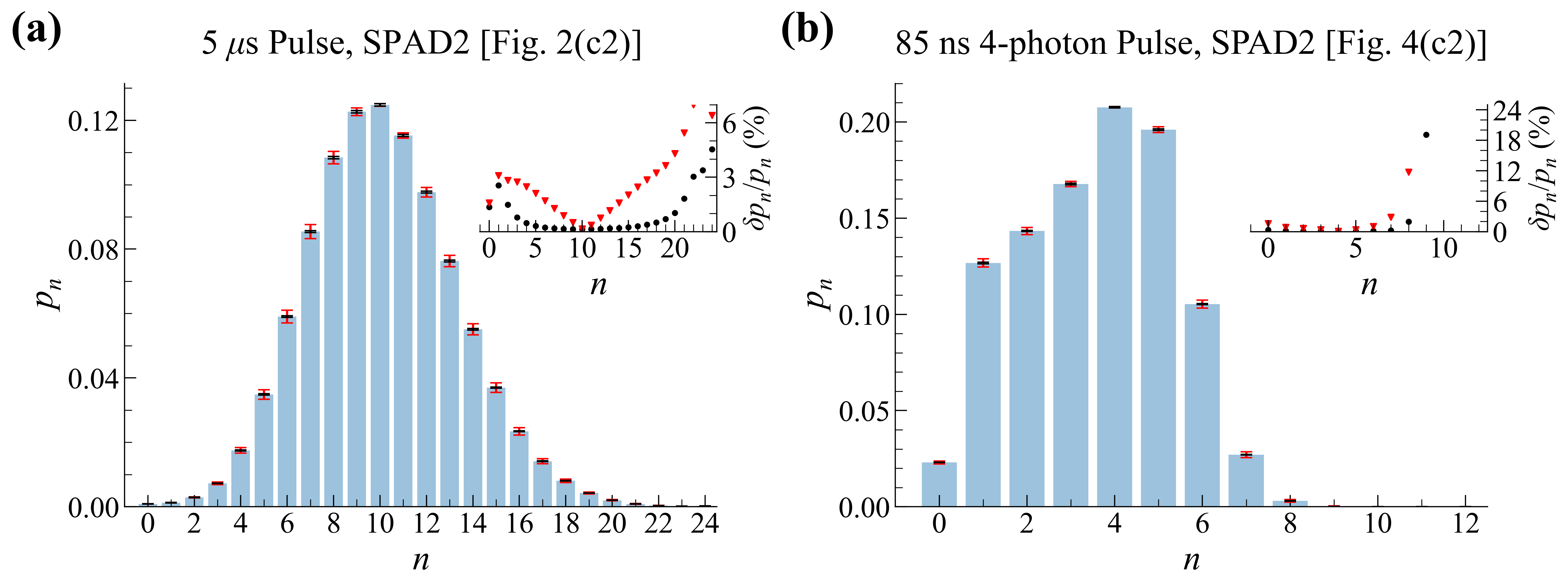
Figure 10: Reconstructions of two of the datasets from the main paper, showing uncertainties in each number component. The left figure is Fig. 2(c2) of the main paper, the reconstruction of a 5 $\mu$s coherent pulse from SPAD2; the right is Fig. 4(c2) of the main paper, the reconstruction of the 85 ns 4-photon coherent pulse from SPAD2. To increase visual clarity, the main figures’ error bars show two standard deviations. As discussed in the text, the black error bars represent statistical uncertainty due only to sampling error, while the expanded red bars show effects due to the detector parameter uncertainties, which are highly correlated across number components. The insets show (one standard deviation) percent uncertainties $\delta p_{n}/p_{n}\times 100$, where $\delta p_{n}$ is the uncertainty in number component $p_{n}$. Black dots indicate sampling error and red triangles indicate additional uncertainty due to uncertainty in detector parameters.

Table 3: Breakdown of contributions to the uncertainties of a few number components of the reconstruction of the 5 $\mu$s SPAD2 coherent pulse. All uncertainties are one standard deviation. As discussed in the main text, the uncertainties from all but sampling error are highly correlated with one another. The quadrature sum of the numbers given matches the total uncertainty $\delta p_{n}$ found by a Monte Carlo simulation with all uncertainties accounted for. We also give the total fractional uncertainty $\delta p_{n}/p_{n}$. The uncertainty contributions from the recovery time effects are zero due to the way we discretize $D(\tau)$, as discussed in the main text, so we omit $\delta\mathbb{R}$ from the table.

Contribution ($\times 10^{-8}$)	$n=2$	$n=6$	$n=10$	$n=14$
Sampling error	4200	14000	17000	11000
$\delta\mathbb{L}$	7200	102000	9900	88000
$\delta\mathbb{B}$	1	21	2	19
$\delta\mathbb{A}$	21	2000	2800	3100
Total, $\delta p_{n}$	8300	103000	20000	89000
$\delta p_{n}/p_{n}$	2.7 %	1.7 %	0.16 %	1.6 %

The insets of Fig. 10 show the percent uncertainties in each component, with the black and red dots corresponding to the black and red error bars of the main figures. For the data in the left panel of Fig. 10, whose reconstruction closely matched the expected Poissonian, the total percent uncertainties, including the correlated uncertainties, stay below 5 % for all components with at least 0.1 % of the reconstructed population. For the right panel of Fig. 10, in which the algorithm failed to reconstruct a Poissonian, the uncertainties on the large-$n$ components are large, perhaps a consequence of the algorithm’s failure to accurately reconstruct. To further quantify the magnitudes of the uncertainties and gain insight in their sources, in Table 3 we give a breakdown of uncertainty by source for several number components of the reconstructed 5 $\mu$s SPAD2 pulse shown in Fig. 10(a). To generate these values, we ran sets of 1,000 Monte Carlo simulations with all uncertainties set to zero except the one under test.

The general form of the sampling error as a function of $n$ is determined by the shape of the measured click distributions. For both of the pulses in Fig. 10, the click distributions are peaked, with a relatively small number of zero-click events, followed by an increase to some maximum number, and then a decrease to zero events for a large number of clicks. Thus the percent uncertainty due to sampling error is large at low and high $n$, but is small at intermediate $n$.

Though the sampling error is a non-negligible contribution for many of the components, the uncertainties due to detector parameters dominates for most number components, as shown in Table 3 and inferred from the insets of Fig. 10. Among these, the uncertainty from the detector efficiency is by far the largest contribution. Though all of our detector parameters’ estimated relative uncertainties are roughly the same (0.1 % to 0.5 %), these uncertainties contribute at different levels because the parameters themselves contribute to the reconstruction at different levels. Since the total effect of afterpulsing is at most $\approx$ 2 % and the total effect of background counts is even smaller in all of our data, the effects of the detector efficiency are the largest corrections we make. We consider the DE an order unity correction, the afterpulsing an order 0.01 correction, and the background counts even smaller. The uncertainty contributions track this hierarchy fairly closely, though afterpulsing becomes more important at larger $n$.

The dead time and recovery time uncertainties contribute nothing to the reconstruction uncertainties, which is due to the way we discretize $D(\tau)$. In constructing this function, we round both $t_{\text{dead}}$ and $t_{\text{rec}}$ to the nearest bin, and then interpolate between these; since the uncertainty in these quantities is much less than the typical bin width of 1 ns, every Monte Carlo simulation chooses the same bins after rounding, resulting in no difference in the matrix $\mathbb{R}$ across simulations.

The uncertainties being dominated by the uncertainty in the detector efficiency largely explains the patterns of fractional uncertainty seen in the insets of Fig. 10. A change in the DE would shift the peak of the reconstructed distribution, so the components on the “sides” of the peak are highly sensitive to changes in the DE, while components near the peak are first-order insensitive. A second effect also plays a part: at larger $n$, generally more factors of the efficiency are involved in the reconstruction, so the large-$n$ components are also increasingly sensitive to changes in the DE. Both of these patterns are visible in the insets of Fig. 10.

For the anti-bunched light reconstructed in this work (Fig. 5 of the main text), we used Monte Carlo simulation in a similar manner as above to investigate the uncertainty on the reconstructed value of $g^{(2)}(0)$. The balance of uncertainties is somewhat different than that of the number components of coherent states above. The primary contribution to the uncertainties on the reconstructed $g^{(2)}$ presented in the main paper is sampling error. This can of course be reduced by taking more data. The next largest contributor, a factor of $2$-$3$ lower, is the uncertainty in the afterpulsing probability. In this work, the detector efficiency uncertainty contributes negligible uncertainty to the reconstructed value of $g^{(2)}$. This is sensible since, theoretically, losses should not affect the value of $g^{(2)}$ [3]. The balance of other effects may be due to our particular setup’s very low efficiency of photon production from our Rydberg ensemble.

C.IV A Note to the User

In our detector characterization efforts detailed in Section B, by far the most involved measurement was that of the detector efficiency, in terms of both time and equipment. Therefore it is worthwhile to consider the consequences of a less-involved efficiency measurement procedure on the reconstructions. We found that with inexpensive commercial power meters we were able to measure the efficiencies of our detectors to $\approx$ 5 % relative uncertainty. We used this relative uncertainty in new Monte Carlo simulations to estimate the resulting uncertainties on the reconstructions. We performed this procedure for several of the pulses of the main text, with results shown in Fig. 11.

Besides the uncertainties on the components all being noticeably larger, the uncertainties also generally increase with larger $n$. This is the same effect as discussed in the last section: heuristically speaking, a number state component $n$ can involve up to $n$ powers of the DE in the reconstruction, so larger $n$ components are more sensitive to variations in the DE. This can give the impression of a larger “average” uncertainty across the reconstructed distribution when the average $n$ is larger.

From this, it is clear that using this tomographic method precisely requires a good detector efficiency measurement.

We also ran the same Monte Carlo simulations on our anti-bunched light data (Fig. 5 of the main text) to investigate the effects on the reconstructed value of $g^{(2)}(0)$. These simulations (not shown) reveal that uncertainty on the detector efficiency, even at the level of 5 %, has negligible effect on the reconstructed $g^{(2)}$. This implies that, if one is seeking to characterize anti-bunched light and is only interested in a value of $g^{(2)}$, one does not need to carefully characterize the detector efficiency. As previously mentioned, our setup produces photons only rarely, and this fact may be responsible for the balance of uncertainties here.

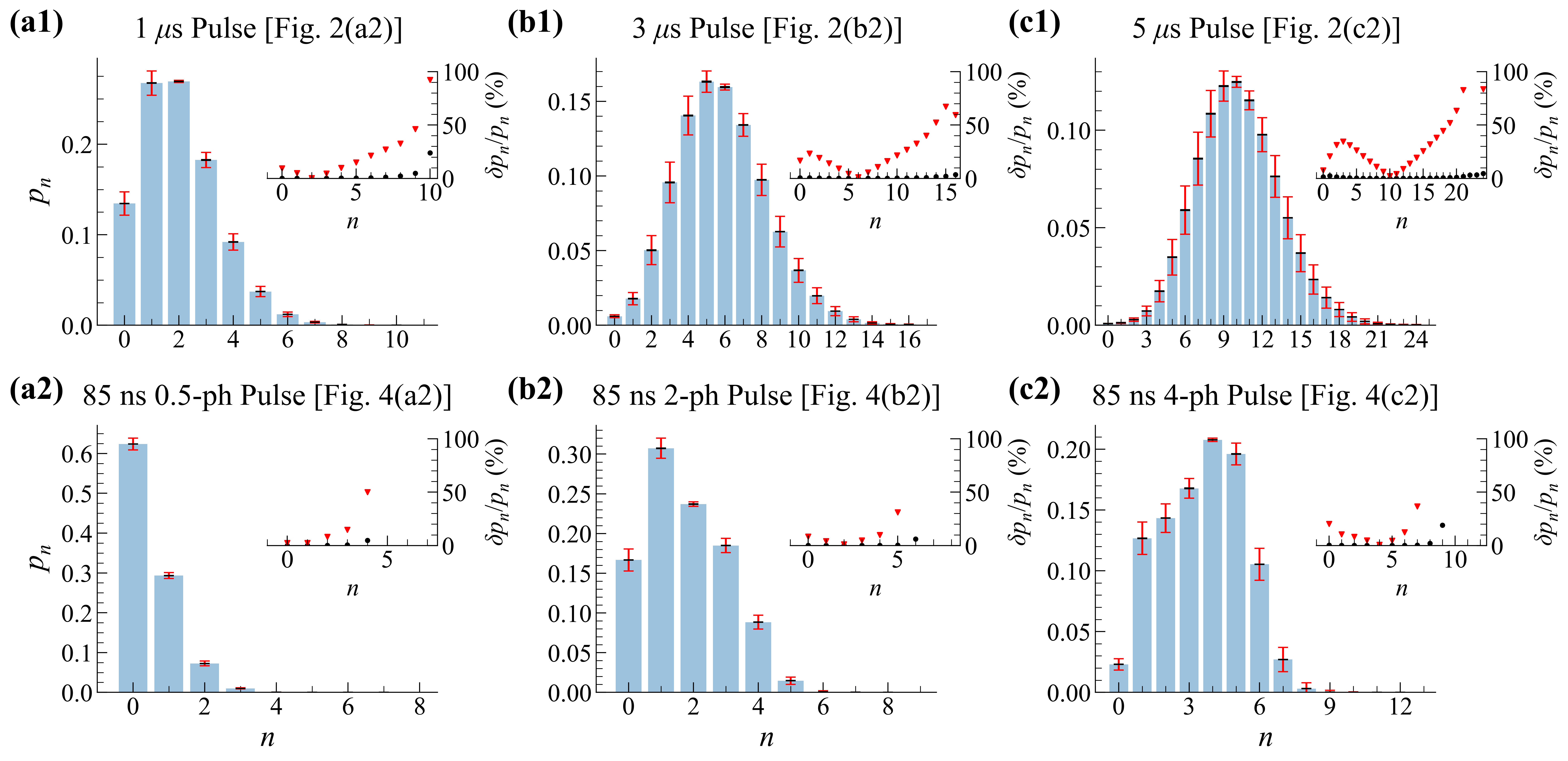
Figure 11: Uncertainties (one standard deviation) on reconstructions when the DE has a relative uncertainty of 5 %. All of these data are from SPAD2, corresponding to Figs. 2 and 4 of the main text, as indicated in the square brackets in each plot’s subtitle: the top row are long coherent pulses (1 $\mu$s, 3 $\mu$s, and 5 $\mu$s from left to right), and the bottom row are short coherent pulses (85 ns, with roughly 0.5 photons, 2 photons, and 4 photons per pulse from left to right). The error bars are one standard deviation; black bars indicate only sampling error, while the expanded red bars indicate the correlated errors due to uncertainties in the detector parameters. The insets show (one standard deviation) percent uncertainties $\delta p_{n}/p_{n}\times 100$, with black dots indicating sampling error and red triangles indicating additional uncertainty due to uncertainty in detector parameters. The notable trend is that the magnitude of the uncertainties gets larger with larger $n$, for both long and short pulses.

References

- [1] P. Banner, “Photon number reconstruction,” GitHub (2023). https://github.com/pbanner/Photon-Number-Reconstruction/.
- [2] A. A. Semenov, A. V. Turchin, and H. V. Gomonay, “Detection of quantum light in the presence of noise,” \JournalTitlePhysical Review A 78, 055803 (2008).
- [3] A. Migdall, S. V. Polyakov, J. Fan, and J. C. Bienfang, eds., Single-Photon Generation and Detection: Physics and Applications (Academic Press, 2013).
- [4] M. Ware, A. Migdall, J. C. Bienfang, and S. V. Polyakov, “Calibrating photon-counting detectors to high accuracy: background and deadtime issues,” \JournalTitleJournal of Modern Optics 54, 361–372 (2007).
- [5] A. W. Ziarkash, S. K. Joshi, M. Stipčević, and R. Ursin, “Comparative study of afterpulsing behavior and models in single photon counting avalanche photo diode detectors,” \JournalTitleSci. Rep. 8, 5076 (2018).
- [6] I. Straka, J. Grygar, J. Hloušek, and M. Ježek, “Counting statistics of actively quenched spads under continuous illumination,” \JournalTitleJournal of Lightwave Technology 38, 4765–4771 (2020).
- [7] F.-X. Wang, W. Chen, Y.-P. Li, D.-Y. He, C. Wang, Y.-G. Han, S. Wang, Z.-Q. Yin, and Z.-F. Han, “Non-markovian property of afterpulsing effect in single-photon avalanche detector,” \JournalTitleJournal of Lightwave Technology 34, 3610–3615 (2016).
- [8] M. A. Wayne, J. C. Bienfang, and S. V. Polyakov, “Simple autocorrelation method for thoroughly characterizing single-photon detectors,” \JournalTitleOpt. Express 25, 20352–20362 (2017).
- [9] L. Mandel and E. Wolf, eds., Optical coherence and quantum optics (Cambridge University Press, 1995).
- [10] Disclaimer: Certain commercial equipment, instruments, or materials are identified in this paper to foster understanding. Such identification does not imply recommendation or endorsement by the National Institute of Standards and Technology, nor does it imply that the materials or equipment identified are necessarily the best available for the purpose.
- [11] N. P. Fox, “Trap detectors and their properties,” \JournalTitleMetrologia 28, 197–202 (1991).
- [12] S. V. Polyakov and A. L. Migdall, “High accuracy verification of a correlated-photon-based method for determining photon-counting detection efficiency,” \JournalTitleOpt. Express 15, 1390–1407 (2007).
- [13] J. M. Houston, C. J. Zarobila, and H. W. Yoon, “Achievement of 0.005% combined transfer uncertainties in the NIST detector calibration facility,” \JournalTitleMetrologia 59, 025001 (2022).
- [14] Z. M. Zhang, T. R. Gentile, A. L. Migdall, and R. U. Datla, “Transmittance measurements for filters of optical density between one and ten,” \JournalTitleApplied Optics 36, 8889 (1997).