Macroscopic distant magnon modes entanglement via a squeezed reservoir

Abstract

The generation of robust entanglement in quantum system arrays is a crucial aspect of the realization of efficient quantum information processing. Recently, the field of quantum magnonics has garnered significant attention as a promising platform for advancing in this direction. In our proposed scheme, we utilize a one-dimensional array of coupled cavities, with each cavity housing a single yttrium iron garnet (YIG) sphere coupled to the cavity mode through magnetic dipole interaction. To induce entanglement between YIGs, we employ a local squeezed reservoir, which provides the necessary nonlinearity for entanglement generation. Our results demonstrate the successful generation of bipartite and tripartite entanglement between distant magnon modes, all achieved through a single quantum reservoir. Furthermore, the steady-state entanglement between magnon modes is robust against magnon dissipation rates and environment temperature. Our results may lead to applications of cavity-magnon arrays in quantum information processing and quantum communication systems.

I Introduction

Quantum entanglement plays a pivotal role in various applications of quantum information processing [1], encompassing quantum cryptography [2], quantum teleportation [3], and quantum metrology [4]. It is a crucial resource for enhancing the performance of quantum devices and technologies [5]. However, preparing long-lived entangled states, especially at the macroscopic scale, becomes challenging due to inevitable interactions between quantum systems and their environments. Consequently, the quest for generating macroscopic entangled states using various physical setups has gained significant attention. In this context, steady-state entanglement between atomic ensembles has been successfully demonstrated [6, 7, 8]. Additionally, entangled states involving macroscopic systems have been reported in different setups, such as entanglement between a single cavity mode and a mechanical resonator in an optomechanical configuration [9]. Recently, experimental achievements include entanglement between two macroscopic resonators coupled to a common cavity mode through optomechanical interaction [10].

Another central challenge in harnessing entanglement to improve various quantum tasks lies in the ability to create and distribute entanglement across large arrays of quantum systems [11, 12, 13, 14, 15, 16, 17]. An intriguing approach to address this challenge is reservoir engineering, where external control drives are used to engineer desirable dissipative dynamics, leading the quantum system to relax in the desired quantum state [18, 19, 14, 20, 21, 22, 23, 24, 25]. However, most reservoir engineering schemes require multiple external control fields to be applied over different elements of the quantum system array [26, 27].

In recent years, hybrid quantum systems, combining different physical subsystems, have received significant attention [28, 29, 30]. Among these systems, cavity magnon setups offer a unique platform to investigate light-matter interactions [31, 32]. In cavity quantum electrodynamics, the strong and ultrastrong coupling between magnons and photons has been increasingly studied [31, 33, 34, 35, 36, 37], with experimental demonstrations of these regimes [38, 39, 40]. This strong coupling opens possibilities for exploring novel phenomena, such as the magnon Kerr effect [41], cavity-magnon polaritons [42], magnon-induced transparency [43], magnomechanically induced slow-light [44], bistability [45], exceptional points [42, 46], magnon blockade [47], and nonreciprocity [48].

Recent proposals aim to realize genuine quantum effects in macroscopic magnon-cavity systems, including magnon blockade [49], magnon squeezed states [50], Schrödinger cat states [51, 52], Bell states [53], and nontrivial bipartite and multipartite entangled states [54, 55]. Of particular interest is the generation of entanglement between distant magnon modes [56], which holds promise for quantum information processing applications. However, to the best of our knowledge, existing studies have primarily focused on entangling only two magnon modes, such as entangling two YIG spheres in a single cavity via Kerr nonlinearity [57], magnetostrictive interaction [58], or applying a vacuum-squeezed drive [59, 60]. Further, stationary quantum entanglement between two massive magnetic spheres can be induced by subjecting each sphere to two-tone Floquet fields, which effectively generates parametric interaction between magnon modes [61]. In the case of two cavities, each containing a single YIG, entanglement between the YIGs has been generated through optomechanical-like coupling [62], vacuum squeezed drive [63], or reservoir engineering [56, 64, 65]. Recently, the bipartite entanglement between magnon modes is investigated in a one-dimensional array of cavities. The entanglement is generated by exploiting the coupling of the magnon modes with a central giant atom via virtual photons [66].

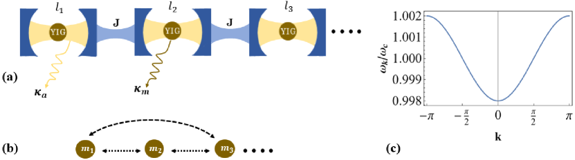
Figure 1: (a) Schematic description of magnon-magnon entanglement generation scheme, consisting of a one-dimensional $2N+1$ array of identical lossy cavities coupled via hopping interaction $J$. Each cavity contains a yttrium iron garnet (YIG) sphere with volume $V$. The cavities’ decay and dissipation rates are $\kappa_{a}$ and $\kappa_{j}$, respectively. The central YIG is coupled to a quantum-squeezed reservoir, enabling our entanglement generation scheme. (b) Describes the effective model, which consists of only magnon modes obtained after removing the cavities via employing Schrieffer-Wolf transformation. (c) shows the behavior of the dispersion relation of the cavity mode in momentum space.

Hybrid quantum magnonic systems hold great promise for efficient quantum networks [67]. Therefore, a crucial task is to establish and control entanglement between multiple magnon modes in arrays based on quantum magnonic systems. In this regard, we propose a scheme to generate entanglement between multiple yttrium iron garnet (YIG) spheres using a reservoir engineering approach with a single squeezed bath. Specifically, our setup consists of an array of cavities, each housing a macroscopic YIG coupled to the cavity through beam splitter-like interaction. However, entanglement cannot be generated with this interaction alone; thus, we introduce the necessary nonlinearity by driving one of the magnon modes with a squeezed reservoir. Previous studies have demonstrated that a single and two-mode squeezed drive can create entanglement between magnon modes [63, 59, 62, 60]. In our work, we show that when one of the magnon modes is subjected to a squeezed reservoir, it is sufficient to generate steady-state bipartite and tripartite entanglement between distant magnon modes.

We would like to highlight that, in principle, the local squeezed reservoir on the central magnon mode ($m_{2}$) can be realized by coupling an auxiliary quantum system. Generation of the squeezed input field can be accomplished using a method similar to the proposal discussed in [68]. For example, the input squeezed reservoir can be engineered by coupling an auxiliary microwave cavity to the central magnon mode through beam-splitter-type interaction. The weak squeezed vacuum field, generated via a flux-driven Josephson parametric amplifier, acts as the driving force for the auxiliary cavity. Consequently, the auxiliary cavity serves as a quantum squeezed reservoir for the central magnon mode [50, 69]. Similarly, the squeezed reservoir can also be achieved by coupling the central magnon mode to a superconducting qubit [70]. More specifically, the approach proposed in  [71] can be implemented by replacing the coplanar waveguide resonator with a YIG placed inside a microwave cavity. This scheme enables the coupling of a superconducting qubit with an adjustable energy gap to a magnon mode characterized by the frequency $\omega_{2}$. By modulating the energy gap of the qubit with a bichromatic field, the squeezed reservoir for the magnon mode can be engineered [50]. Alternatively, the input squeezed radiation can be generated by applying a two-tone microwave field drive to the central YIG, where the magnon mode is coupled to its mechanical vibrational mode through magnetostrictive interaction [72, 73].

The paper is structured into the following sections: In Sec. II, we introduce the model; and in Sec. III derivation of effective Hamiltonian is presented. The results for bipartite and tripartite entanglement between the magnon modes are discussed in Secs. IV.1 and IV.2, respectively. Finally, in Sec. V, we offer concluding remarks and summarize the key findings.

II The Model

We investigate a cavity-magnon system comprising a one-dimensional array of $2N+1$ cavities, as illustrated in Fig. 1. These cavities are interconnected through photon-hopping interactions. Inside each cavity, a single YIG sphere is present, coupled to the cavity mode via magnetic dipole interaction. In this study, we consider a single magnon mode, which represents quasi-particles with collective spin excitations, associated with each YIG in the cavities. The Hamiltonian governing the field for the cavity array is as follows:

$$H_{a}/\hbar= \omega_{c}\sum_{j}\hat{a}^{\dagger}_{j}\hat{a}_{j}-J\sum_{j}(\hat{a}_{j}\hat{a}_{j+1}^{\dagger}+\hat{a}_{j}^{\dagger}\hat{a}_{j+1}).$$ (1)

The first term represents the free energy of the cavities, while the second term accounts for the exchange energy of the field. $\hat{a}_{j}$ and $\hat{a}_{j}^{\dagger}$ are the bosonic annihilation and creation operators of the $j$-th cavity and the corresponding resonance frequency $\omega_{c}$. Here $j$ ($j=-N,..,0,...,N$) describes the index of the cavity in a one-dimensional array, with each cavity interconnected through a hopping coupling called $J$. We consider only a single photon process in each cavity.

The ferromagnetic sample (YIG) holds within it scattering spin waves, with the assumption that only the spatially uniform Kittel mode [74] exhibits a pronounced interaction with photons within the cavity. The free Hamiltonian for these magnon modes is given by

$$H_{m}/\hbar=\sum_{n}\omega_{n}\hat{m}^{{\dagger}}_{n}\hat{m}_{n},$$ (2)

here $\hat{m}_{n}$ ($\hat{m}^{{\dagger}}_{n}$) is the annihilation (creation) operator of the magnon mode, and $\omega_{n}$ is the associated frequency of the mode. In addition, the index $n$ in the summation is an integer number such that $n\in[-N,N]$. In general, some cavities can be empty while some can contain YIG spheres. For example, in Sec. IV, we assume that three of the cavities are occupied while the rest remain empty. In this scenario, Eq. (2) includes only three terms for magnon modes, however, $2N+1$ cavities are present. The magnon frequencies can be calculated based on the applied magnetic fields $H_{n}$, and given by $\omega_{n}=\gamma H_{n}$, where $\gamma/2\pi=28$ GHz/T represents the gyromagnetic ratio. The interaction between the magnon and cavity modes is given by

$$H_{I}/\hbar=\sum_{n}g_{n}(\hat{a}_{n}\hat{m}^{{\dagger}}_{n}+\hat{a}^{{\dagger}}_{n}\hat{m}_{n}),$$ (3)

here, $g_{n}$ is the coupling strength between the magnon and associated cavity modes and is given by $g_{n}=\zeta\gamma/2\sqrt{5\hbar\omega_{n}\mu_{0}N/V}$. The volume of the cavity is given by $V$, $N$ represents the total number of spins in the YIG, $\mu_{0}$ is the permeability of free space, and $\zeta$ describes the spatial overlap between the magnon and photon modes. We note that the interaction term in Eq. (3) is obtained after performing the Holstein-Primakoff transformation in which collective spin operators are written in the form of bosonic magnon operators $\hat{m}$ ($\hat{m}^{\dagger}$) [57]. In addition, the counter-rotating terms $\hat{m}\hat{a},\hat{m}^{\dagger}\hat{a}^{\dagger}$ are ignored assuming the validity of rotating wave approximation [59]

III The Schrieffer–Wolff Approximation and Effective Hamiltonian

To generate entanglement between two magnon modes, a nonlinear interaction such as effective parametric-type nonlinear coupling $(\hat{m}_{1}^{\dagger}\hat{m}_{2}^{\dagger}+\hat{m}_{1}\hat{m}_{2})$ between the modes is required. This interaction can be achieved by introducing strong Kerr nonlinearity [57] or nonlinear magnomechanical interaction [58]. It is typically easier to engineer an effective beamsplitter-type coupling $(\hat{m}_{1}^{\dagger}\hat{m}_{2}+\hat{m}_{1}\hat{m}_{2}^{\dagger})$ between the magnon modes. For instance, in a system with two YIGs spheres placed inside a microwave cavity, it is possible to generate the desired coupling $(\hat{m}_{1}^{\dagger}\hat{m}_{2}+\hat{m}_{1}\hat{m}_{2}^{\dagger})$ by carefully selecting the system parameters that allow adiabatic elimination of the cavity mode [75]. Another approach involves an array of three cavities, where the central cavity contains a qubit, and each end cavity houses a YIG sample [65]. By employing the dispersive regime and using the Schrieffer-Wolff (Frohlich-Nakajima) approximation [76, 77, 78], the cavity modes can be eliminated, resulting in an effective beamsplitter-type coupling between the magnon modes. In our case, we adopt the latter method to create an array of YIGs with an effective coherent coupling $(\hat{m}_{n}^{\dagger}\hat{m}_{n+1}+\hat{m}_{n}\hat{m}_{n+1}^{\dagger})$. Our strategy is to utilize these easier-to-engineer beam-splitter-type magnon-magnon interactions but introduce the required nonlinearity for generating entanglement between distant magnon modes through a squeezed thermal bath [68, 79, 80, 81, 82].

The Hamiltonian $H_{a}$ (Eq. (1)) associated with a one-dimensional array of coupled cavities represents the tight-binding bosonic model. To diagonalize it, we introduce new operators in the momentum space ($k$-space). The resulting diagonal Hamiltonian is given by

$$H_{\text{diag}}/\hbar=\sum_{k}\omega_{k}\hat{a}^{\dagger}_{k}\hat{a}_{k},$$ (4)

here, we have introduced

$$\hat{a}_{k}= \frac{1}{\sqrt{2N+1}}\sum_{j}\hat{a}_{j}e^{ikj},$$ (5)

$$\hat{a}^{\dagger}_{k}= \frac{1}{\sqrt{2N+1}}\sum_{j}\hat{a}^{\dagger}_{j}e^{-ikj}.$$ (6)

We have assumed the periodic boundary conditions such that $k:=k_{m}=2\pi m/(2N+1)$ with $m\in[-N,N]$, and considering a large cavity array ($N\gg 1$) results in $k\in[-\pi,\pi]$. Moreover, $\omega_{k}=\omega_{c}-2J\text{cos}k$ is the dispersion relation of the cavity mode. The interaction Hamiltonian, as presented in Eq. (3), modifies to

$$H_{I}/\hbar=\frac{1}{\sqrt{2N+1}}\sum_{k,n}\left[g_{n}(\hat{a}_{k}\hat{m}^{{\dagger}}_{n}e^{ikl_{n}}+\hat{a}_{k}^{{\dagger}}\hat{m}_{n}e^{-ikl_{n}})\right].$$ (7)

We note that $l_{n}=n$, and it is associated with the position of the YIG in the array (see Fig. 1). To derive an effective Hamiltonian involving only magnon modes, the elimination of cavity modes is necessary. This can be accomplished by invoking the Schrieffer-Wolf (Frohlich-Nakajima) transformation [76, 77, 83, 84].

$$[S,H_{0}]=-H_{I}.$$ (8)

Where $H_{0}$ is the free Hamiltonian consisting of cavity ($H_{\text{diag}}$), and magnon ($H_{m}$) modes. In addition, $H_{I}$ is the interaction Hamiltonian between the cavity and magnon modes, as given in Eq. (7). $S$ is called a generator and it is anti-Hermitian in nature i.e., $S^{\dagger}=-S$, and it is given by

$$S=\sum_{k,n^{\prime}}\left[\alpha_{k}^{n^{\prime}}\hat{a}_{k}\hat{m}_{n^{\prime}}^{\dagger}-{\alpha_{k}^{n^{\prime}}}^{\star}\hat{a}^{\dagger}_{k}\hat{m}_{n^{\prime}}\right],$$ (9)

here $\alpha_{k}^{n^{\prime}}=g_{n^{\prime}}/(\sqrt{2N+1}(\omega_{n^{\prime}}-\omega_{k}))e^{-ikl_{n^{\prime}}}$. The effective Hamiltonian of the system can be determined by unitary transformation $e^{S}He^{-S}$. In the dispersive regime, such that $\omega_{n^{\prime}}-\omega_{k}\gg g_{n^{\prime}}/\sqrt{2N+1}$, we can ignore higher order terms in the expansion of the unitary transformation, i.e., $H_{0}+1/2[H_{I},S]$, and keep terms up to the second order in $\alpha_{k}^{n^{\prime}}$. Consequently, the approximate effective Hamiltonian, comprising solely of magnon modes, can be explicitly expressed as follows [85, 65, 86, 66]:

$$H_{\text{eff}}/\hbar= \sum_{n}\omega^{\prime}_{n}\hat{m}_{n}^{\dagger}\hat{m}_{n}+\sum_{n,n^{\prime}}\mathcal{G}_{nn^{\prime}}(\hat{m}_{n}^{\dagger}\hat{m}_{n^{\prime}}+\hat{m}_{n}\hat{m}^{\dagger}_{n^{\prime}}).$$ (10)

Where we have replaced discrete modes with a continuous distribution

$$\frac{1}{2N+1}\sum_{k}=\frac{1}{2\pi}\int_{-\pi}^{\pi}dk,$$ (11)

in addition, the following integral identity is employed in the derivation of Eq. (10)

$$\int_{-\pi}^{\pi}\frac{dk}{2\pi}\frac{e^{-ilx}}{U+V\text{cosx}}=(-1)^{|l|}\sqrt{\frac{1}{U^{2}-V^{2}}}e^{-|l|\text{arccosh}(U/V)}.$$ (12)

The effective frequency $\omega^{\prime}_{n}$ of the $n$-th magnon mode is given by

$$\omega^{\prime}_{n} =\omega_{n}+\frac{g^{2}_{n}}{\sqrt{\Delta_{n}^{2}+4J\Delta_{n}}},\text{and}$$ (13)

$$\mathcal{G}_{nn^{\prime}} =\frac{g_{n}g_{n^{\prime}}(-1)^{\mid l_{nn^{\prime}}\mid}}{2}\bigg{(}\frac{e^{-|l_{nn^{\prime}}|\text{arccosh}{(1+\Delta_{n^{\prime}}}/2J)}}{\sqrt{\Delta_{n^{\prime}}^{2}+4J\Delta_{n^{\prime}}}}+$$

$$\qquad\qquad\qquad\frac{e^{-|l_{nn^{\prime}}|\text{arccosh}{(1+\Delta_{n}}/2J)}}{\sqrt{\Delta_{n}^{2}+4J\Delta_{n}}}\bigg{)},$$ (14)

is spatially dependent effective coupling strength between the magnon modes. Further, $\Delta_{n^{\prime}}=(\omega_{n^{\prime}}-\delta_{a})^{2}+4J(\omega_{n^{\prime}}-\delta_{a})$, $\Delta_{n}=(\omega_{n}-\delta_{a})^{2}+4J(\omega_{n}-\delta_{a})$, and $\delta_{a}=\omega_{a}-2J$ is the lower bound frequency of the cavity mode. In addition, $l_{nn^{\prime}}=l_{n}-l_{n^{\prime}}$ is the distance between $n$-th and $n^{\prime}$-th YIG placed inside the cavity array. In our numerical simulations, we consider identical magnon modes: Since all the YIGs oscillate inside the cavity with the same frequency, therefore, resonance condition $\Delta_{n^{\prime}}$ = $\Delta_{n}=\Delta$, and $\delta_{n^{\prime}}$= $\omega_{n^{\prime}}-\omega_{a}$ and $\delta_{n}=\omega_{n}-\omega_{a}=\delta$. The effective Hamiltonian in Eq. (10) takes on the form of a beam splitter for magnon modes, which can be used for state transfer between distant magnon modes, as discussed in the previous studies [65, 66]. We note that, in our case, the interaction between magnon modes is mediated by virtual photons; and when contrasted with actual photons, virtual photons possess the advantages of being non-propagating and non-radiative. Consequently, energy exchange facilitated by virtual photons results in entirely coherent dynamics devoid of dissipation [65].

IV Results

To illustrate the working principles of our scheme, we initially focus on a simple scenario where only three cavities are occupied, each containing one YIG. The remaining cavities in the array are unoccupied. It is worth noting that the placement of YIGs is not restricted to neighboring cavities; they can be situated in any of the three cavities within the array. In addition, we consider a squeezed thermal reservoir coupled to the central YIG. It is worth noting that this entanglement generation scheme remains applicable for arrays with arbitrary cavities lengths [68].

We employ the quantum Langevin equations to describe the system’s dynamics. By working in the interaction picture through the unitary evolution operator $\hat{U}(t)=\text{exp}[-it(\sum_{n}\omega^{\prime}_{n}\hat{m}^{\dagger}_{n}\hat{m}_{n})]$, the equations of motion take the following form (for convenience, we will now omit the hat symbol from operators)

$$\dot{m_{1}}= -\kappa_{1}m_{1}-i\mathcal{G}_{12}m_{2}-i\mathcal{G}_{13}m_{3}+\sqrt{2\kappa_{{}_{1}}}m^{\text{in}}_{1},$$

$$\dot{m_{2}}= -\kappa_{2}m_{2}-i\mathcal{G}_{12}m_{1}-i\mathcal{G}_{23}m_{3}+\sqrt{2\kappa_{2}}m^{\text{in}}_{2},$$

$$\dot{m_{3}}= -\kappa_{3}m_{3}-i\mathcal{G}_{13}m_{1}-i\mathcal{G}_{23}m_{2}+\sqrt{2\kappa_{{}_{3}}}m^{\text{in}}_{3}.$$ (15)

Here, $\kappa_{n}$ is the dissipation rate of the $n$-th magnon modes, and $m^{in}_{n}$ represents the corresponding input noise operator. The input noise operator $m^{\text{in}}_{2}$ accounts for driving the central magnon mode through a squeezed vacuum field. It is characterized by zero mean and following correlation functions [87]

$$\langle m^{\text{in}}_{2}(t)m_{2}^{\text{in}{\dagger}}(t^{\prime})\rangle= (\mathcal{N}+1)\delta(t-t^{\prime}),$$

$$\langle m^{\text{in}{\dagger}}_{2}(t)m_{2}^{\text{in}}(t^{\prime})\rangle= \mathcal{N}\delta(t-t^{\prime}),$$

$$\langle m^{\text{in}}_{2}(t)m_{2}^{\text{in}}(t^{\prime})\rangle= \mathcal{M}\delta(t-t^{\prime}),$$

$$\langle m^{\text{in}{\dagger}}_{2}(t)m_{2}^{\text{in}{\dagger}}(t^{\prime})\rangle= \mathcal{M}^{*}\delta(t-t^{\prime}).$$ (16)

Here $\mathcal{N}=\sinh^{2}{r}+\bar{n}_{2}(\sinh^{2}r+\cosh^{2}{r})$ and $\mathcal{M}$= $e^{i\theta}\sinh{r}\cosh{r}(1+2\bar{n}_{2})$ with $\theta$ and $r$ being the phase and squeezing parameter of the input squeezed reservoir, respectively. In addition, $\mathcal{N}$ and $\mathcal{M}$ account for the number of excitations and correlations, respectively. We observe that due to the Schrieffer-Wolf transformation as described in Eq. (9), additional terms are introduced into the bath correlation function. Nonetheless, the alterations induced by this transformation in the correlation function are deemed negligible. Among these parameters, $\mathcal{M}$ plays the most influential role in entanglement generation. The equilibrium mean thermal magnon number can be determined by $\bar{n}_{2}(\omega_{2})=[\exp(\hbar\omega_{2}/K_{B}T_{2})-1]^{-1}$.

The input noise operators for the other two magnon modes are characterized by the following correlation functions

$$\langle m^{\text{in}}_{\alpha}(t)m_{\alpha}^{\text{in}{\dagger}}(t^{\prime})\rangle= (\bar{n}_{\alpha}+1)\delta(t-t^{\prime}),$$

$$\langle m^{\text{in}{\dagger}}_{\alpha}(t)m_{\alpha}^{\text{in}}(t^{\prime})\rangle= \bar{n}_{\alpha}\delta(t-t^{\prime}),$$ (17)

here $\alpha=1,3$, and $\bar{n}_{\alpha}=[\exp(\hbar\omega_{\alpha}/K_{B}T_{\alpha})-1]^{-1}$.

In our scheme, we showcase the possibility of generating entanglement between all potential bipartitions of the magnon modes by driving the central magnon mode with an input quantum-squeezed field. The quadratures for both the magnon modes and the input noise operators are defined as follows $x_{n}=(m_{n}+m_{n}^{\dagger})/\sqrt{2}$, $y_{n}=(m_{n}-m_{n}^{\dagger})/\sqrt{2}i$, and $x^{in}_{n}=(m^{in}_{n}+m^{in{\dagger}}_{n})/\sqrt{2}$, $y_{n}=(m^{in}_{n}-m^{in{\dagger}}_{n})/\sqrt{2}i$, respectively. In terms of quadrature fluctuations, the quantum Langevin equation (IV) can be rewritten as

$$\dot{F}(t)=F(t)A+N(t),$$ (18)

where $F(t)$=[$x_{1}(t)$, $y_{1}(t)$, $x_{2}(t)$, $y_{2}(t)$, $x_{3}(t)$, $y_{3}(t)]^{T}$, and $N(t)$=[$x^{in}_{1}(t)$, $y^{in}_{1}(t)$, $x^{in}_{2}(t)$, $y^{in}_{2}(t)$, $x^{in}_{3}(t)$, $y^{in}_{3}(t)]^{T}$ denote the quadrature fluctuation vectors of magnon and input noise operators, respectively. The drift matrix $F$ is given by

$$F=\begin{pmatrix}-\kappa_{1}&0&0&\mathcal{G}_{12}&0&\mathcal{G}_{13}\\ 0&-\kappa_{1}&-\mathcal{G}_{12}&0&-\mathcal{G}_{13}&0\\ 0&\mathcal{G}_{12}&-\kappa_{2}&0&0&\mathcal{G}_{23}\\ -\mathcal{G}_{12}&0&0&-\kappa_{2}&-\mathcal{G}_{23}&0\\ 0&\mathcal{G}_{13}&0&\mathcal{G}_{23}&-\kappa_{3}&0\\ -\mathcal{G}_{13}&0&-\mathcal{G}_{23}&0&0&-\kappa_{3}\end{pmatrix}.$$ (19)

As the effective Hamiltonian of the magnon modes, as given in Eq. (10), is quadratic, and the input quantum noise is Gaussian, as a result, the state of the system also remains Gaussian. The reduced state, consisting of three magnon modes, forms a continuous variable three-mode Gaussian state. This state can be entirely characterized by a $6\times 6$ covariance matrix $V$, which is expressed as

$$V_{ij}=\frac{1}{2}\left\langle F_{i}(t)F_{j}(t)+F_{j}(t)F_{i}(t)\right\rangle\quad i,j=1,2,\dots,6.$$ (20)

The steady-state solution can be obtained by solving the Lyapunov equation

$$FV+VF^{T}=-D$$ (21)

where $D$ is the diffusion matrix and can be derived from the noise correlation matrix; $\langle N_{i}(t)N_{j}(t)+N_{j}(t)N_{i}(t)\rangle/2=D_{ij}\delta((t-t^{\prime})$. It can be written as a direct sum of $D=D_{1}\oplus D_{2}\oplus D_{3}$, with $D_{\alpha}=\text{diag}[\kappa_{\alpha}(2\bar{n}_{\alpha}+1),\kappa_{\alpha}(2\bar{n}_{\alpha}+1)]$, and

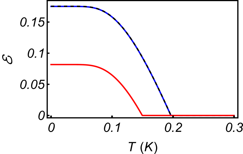
Figure 2: Magnon-magnon bipartite entanglement as a function of the environment temperature $T$. The blue solid line represents the logarithmic negativity $\mathcal{E}_{1,2}$, between $m_{1}$ and $m_{2}$ modes, while the black dashed line indicates the logarithmic negativity $\mathcal{E}_{2,3}$ between $m_{2}$ and $m_{3}$ modes. Further, the red solid line shows the logarithmic negativity $\mathcal{E}_{1,3}$ between $m_{1}$ and $m_{3}$ modes. Parameters: $\omega_{n}/2\pi=10$ GHz, $g_{j}/2\pi=10$ MHz, $J/2\pi=12$ MHz, $\kappa_{n}/2\pi$=$5$ MHz, and $r=1$.

$$D_{2}=\begin{pmatrix}\kappa_{2}\mathcal{U}_{1}&i\kappa_{2}(\mathcal{M}^{*}-\mathcal{M})\\ i\kappa_{2}(\mathcal{M}^{*}-\mathcal{M})&\kappa_{2}\mathcal{U}_{2}\end{pmatrix}.$$ (22)

where $\mathcal{U}_{1}=(2\mathcal{N}+1+\mathcal{M}+\mathcal{M}^{*})$, and $\mathcal{U}_{2}=(2\mathcal{N}+1-\mathcal{M}-\mathcal{M}^{*})$.

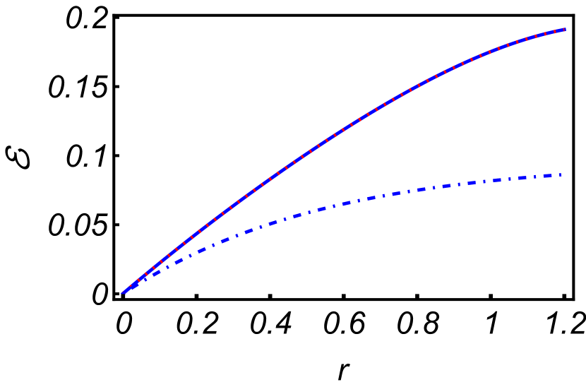
Figure 3: Magnon-magnon bipartite entanglement $\mathcal{E}$ as a function of squeezing parameter $r$. The solid blue line illustrates the logarithmic negativity $\mathcal{E}_{1,2}$ characterizing the entanglement between $m_{1}$ and $m_{2}$ magnon modes. The red dashed curve showcases the logarithmic negativity $\mathcal{E}_{2,3}$ representing the entanglement between the $m_{2}$ and $m_{3}$ modes. Furthermore, the blue dot-dashed line shows the logarithmic negativity $\mathcal{E}_{1,3}$ between $m_{1}$ and $m_{3}$ considering the same parameters as those specified in Fig. 2.

IV.1 Bipartite entanglement

To investigate the entanglement between the magnon modes, we compute the logarithmic negativity $\mathcal{E}_{N}$. This quantity has previously been proposed as a measure of entanglement and helps establish the conditions under which the two modes are entangled [88]. In the continuous variable case, the logarithmic negativity is defined as [89]

$$\mathcal{E}=\text{max}[0,-\ln 2\mathcal{V_{-}}],$$ (23)

where $\mathcal{V_{-}}=\sqrt{1/2(\Sigma-(\Sigma^{2}-4\det V^{\prime})^{1/2}}$ with $\Sigma=\det A+\det B-2\det C$. $V^{\prime}$ is a $4\times 4$ matrix obtained from steady-state covariance matrix $V$ by removing the two rows and associated columns related to the traced-out magnon mode. The reduced covariance matrix $V^{\prime}$ is given by

$$V^{\prime}=\begin{pmatrix}A&C\\ C^{T}&B\end{pmatrix}.$$

We compute the bipartite entanglement among all possible pairs of magnon modes by employing the logarithmic negativity $\mathcal{E}_{N}$. The analytical solution of equation (21) is too cumbersome and we don’t report it here. Instead, we extensively examine the logarithmic negativity across various system parameters. For numerical evaluations, we employ experimentally attainable parameters reported in recent studies [90, 91, 92, 93, 55]. We consider the magnon density at low temperature with ground state spin $s=5/2$ of the $Fe^{+}_{3}$ ion in the YIG sphere. The total number of spins $N=\rho V$ with $\rho=4.22\times 10^{27}/m^{3}$ characterizing the density of each YIG and $V$ is the volume of each sphere with diameter 250 $\mu$-meter; this results in the total number of spins $N=3.5\times 10^{6}$ in each YIG.

In Fig. 2, we present a plot illustrating bipartite entanglement, quantified using the logarithmic negativity, among all possible pairs of magnon modes within an effective system comprising three magnon modes. These results are derived using a set of experimentally feasible parameters [43]: $\omega_{n}/2\pi=10$ GHz, $g_{j}/2\pi=10$ MHz, $J/2\pi=12$ MHz, $\omega_{c}/2\pi=10$ GHz, $\kappa_{1}/2\pi$=$\kappa_{3}/2\pi$= $5$ MHz, $r=1$, and the phase angle $\theta=0$. The entanglement is robust against temperature and survives up to about $T=0.2$ K (solid blue line and dashed black line), and $T=0.15$ K (red solid line). The coupling $\mathcal{G}_{13}$ between YIG1 and YIG3 is relatively weak as compared to $\mathcal{G}_{12}$ or $\mathcal{G}_{23}$ due to their farthest location and as a result, YIG1 and YIG3 are relatively weakly entangled described by red line in Fig. 2. However, the more pronounced squeezing parameter $r$ would result in a more robust entanglement against the environment temperature. Here, we consider a reasonable value of the squeezing parameter $r=1$. The logarithmic negativity $\mathcal{E}_{1,2}$ between YIG1 and YIG2 and $\mathcal{E}_{2,3}$ between YIG2 and YIG3 are the same due to the same couplings; $\mathcal{G}_{12}$= $\mathcal{G}_{23}$ represented by solid blue and black dashed lines. The quantum squeezed reservoir coupled to the central magnon mode is responsible for entanglement generation between the magnon modes. The degree of entanglement decreases by reducing the squeezing parameter $r$ and dies out in the absence of the squeezed reservoir. We observe that the difference in the order of magnon decays at resonance frequencies can produce significant changes in the amount of steady-state entanglement between the two magnon modes. Each magnon-pair has a state-swap interaction and the squeezing can be transferred from a squeezed magnon state to another magnon state. As a result, each magnon pair is to be entangled due to swap-state type interaction via squeezing. This implies that squeezing can affect the bipartite entanglement generated in between a pair of the magnon modes.

To observe the impact of squeezing on entanglement generation, we plot the bipartite entanglement, quantified using logarithmic negativity ($\mathcal{E}$), as a function of the squeezing parameter ($r$). This can be observed in Fig. 3. The results indicate that without the presence of the squeezed thermal bath, entanglement generation within our scheme is unattainable. Therefore, it is evident that squeezing plays a pivotal role in the generation of entanglement, with logarithmic negativity exhibiting a notable increase as the squeezing parameter ($r$) is raised. The entanglement between the magnon modes $m_{1}$-$m_{2}$ and $m_{2}$-$m_{3}$ is identical, owing to the equal coupling strength between these magnon pairs. However, the magnon modes $m_{1}$-$m_{3}$ are relatively weakly coupled, primarily because of the greater distance between the associated YIGs. Consequently, the entanglement $\mathcal{E}_{m_{1},m_{3}}$ between modes $m_{1}$-$m_{3}$ is lower in comparison to the other two pairs.

IV.2 Tripartite entanglement

We further investigate the possibility of the generation of the distant magnon-magnon tripartite entanglement in the array as shown in Fig. 1. To this end, we employ the minimal residual contangle given by [94, 95]

$$\mathcal{R}_{i|jk}=C_{i|jk}-C_{i|j}-C_{i|k}.$$ (24)

Here, the contangle of subsystems $x$ and $y$ is denoted by $C_{x|y}$, and $y$ may represent more than one mode. $C_{x|y}$ is a proper entanglement monotone, and it is determined by the square of the logarithmic negativity between the respective modes, which is given by

$$\mathcal{E}_{i|jk}=\text{max}[0,-\ln 2\mathcal{V}_{i|jk}],$$ (25)

where $\mathcal{V}_{i|jk}=\text{min}\absolutevalue{\text{eig}i\Omega_{3}\tilde{V}}$ is the smallest symplectic eigenvalues. $\Omega_{3}$ is the symplectic matrix $\Omega_{3}=\oplus^{3}_{j=1}i\sigma_{y}$, with $\sigma_{y}$ being the $y$-Pauli matrix and $\oplus$ symbol describes the direct sum of the $\sigma_{y}$ matrices. The $6\times 6$ covariance matrix $\tilde{V}$ is obtained by inverting the momentum quadrature of one of the magnon modes. The transformed covariance matrix $\tilde{V}$ is determined by $\tilde{V}=P_{i|jk}VP_{i|jk}$ where $P_{1|23}=\text{diag}[1,-1,1,1,1,1]$, $P_{2|13}=\text{diag}[1,1,1,-1,1,1]$, and $P_{3|12}=\text{diag}[1,1,1,1,1,-1]$ are partial transposition diagonal matrices. The steady state of the magnon modes can be fully characterized by the $6\times 6$ covariance matrix because of its Gaussian nature. The tripartite entanglement for Gaussian states can be determined by minimum residual cotangle [94, 95]

$$\mathcal{R}_{\text{min}}=\text{min}[\mathcal{R}_{1|23},\mathcal{R}_{2|13},\mathcal{R}_{3|12}].$$ (26)

This ensures that the tripartite entanglement remains unchanged regardless of how the modes are permuted.

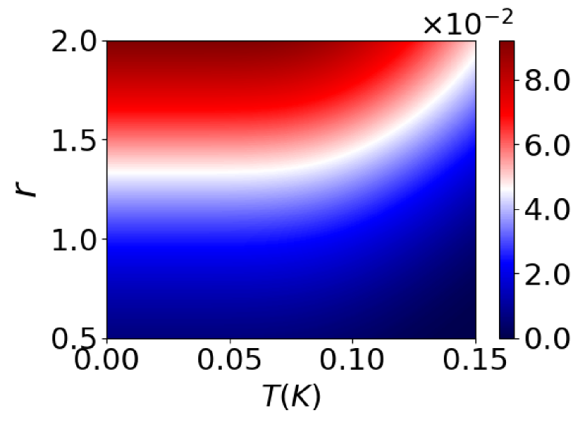
Figure 4: Two-dimensional plot for tripartite entanglement, quantified by minimal residual contangle $\mathcal{R}$ as a function of bath temperature $T$, and squeezing parameter $r$. The rest of the system parameters are the same as given in Fig. 2.

The density plot of magnon-magnon tripartite entanglement determined via minimum residual cotangle $\mathcal{R}_{\text{min}}$ is shown in Fig. 4. It is evident from the results that considerable tripartite entanglement can be generated between magnon modes when the central magnon mode is coupled to a squeezed reservoir. Fig. 4 shows that the degree of entanglement is significantly enhanced with the increase in the squeezing parameter $r$.

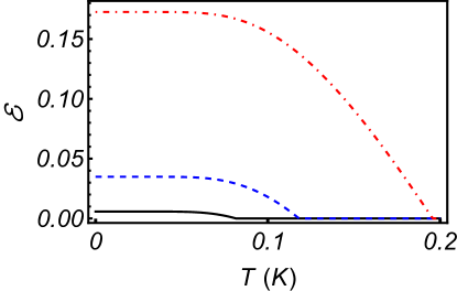
(a)

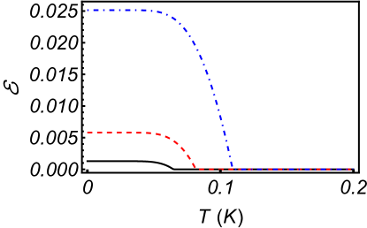
(b)

Figure 5: (Color online). In the given panel, the pairs of bipartite entanglement for a 5-YIG sample are shown. (a) The black solid, blue dashed, and red dotdashed lines indicate the entanglement between $m_{1}$ and $m_{4}$ modes, $m_{2}$ and $m_{4}$, and $m_{3}$ and $m_{4}$, respectively. (b) Describes the bipartite entanglement between $m1$ and $m_{5}$ (solid black curve), $m_{2}$ and $m_{5}$ (red dashed curve), $m_{3}$ and $m_{5}$ blue dotdashed Curve. The parameters remain the same as used in Fig. 3

V Conclusion

In summary, we have shown that steady-state bipartite and tripartite entanglement can be generated between distant magnon modes when only one of these magnon modes is coupled to a quantum-squeezed reservoir. In particular, we considered an array of $N$ cavities each of which houses a single YIG sphere, and the central YIG is coupled to a single-mode squeezed vacuum bath. We have demonstrated that steady-state bipartite and tripartite entanglement can be generated among magnon modes hosted by YIGs when some of the cavities, up to five, are occupied. In contrast to prior proposals for magnon-magnon entanglement generation [58, 59, 63, 56, 57, 62, 64, 65, 60], both bipartite and tripartite entanglement are possible in our scheme. Further, in principle, our scheme can be extended to an arbitrary number of YIGs within the cavity array [68, 81]. However, achieving entanglement across the entire array may necessitate negligible or extremely small magnon decay rates. To address this challenge, we propose the use of an external squeezed drive on each cavity in the array, enabling strong long-range interactions between YIGs positioned at greater distances within the array [86]. In our scheme, the entanglement generation does not require nonlinearity, instead, entanglement is generated via a squeezed reservoir and its strength depends on the squeezing parameter $r$. The generated entanglement is robust against the environment temperature provided the magnons dissipation rates are sufficiently low. It may be interesting to look for multipartite entangled states of magnons, which is left for future works. Our work may be useful in designing quantum networks based on cavity-magnon systems [67].

Appendix A Bipartite entanglement with five YIGs

Here, we extend our results for five YIGs placed inside the cavities array, and the squeezed reservoir is coupled to the central YIG. The Langevin equations of motion in this case are given by

$$\dot{m_{1}}= -\kappa_{1}m_{1}-i\sum_{n^{\prime}=2}^{5}\mathcal{G}_{1n^{\prime}}m_{n^{\prime}}+\sqrt{2\kappa_{1}}m_{1_{in}},$$

$$\dot{m_{2}}= -\kappa_{2}m_{2}-i\mathcal{G}_{12}m_{1}-i\sum_{n^{\prime}=3}^{5}\mathcal{G}_{2n^{\prime}}m_{n^{\prime}}+\sqrt{2\kappa_{2}}m_{2_{in}},$$

$$\dot{m_{3}}= -\kappa_{3}m_{3}-i\sum_{n=1}^{2}\mathcal{G}_{n3}m_{3}-i\sum_{n^{\prime}=4}^{5}\mathcal{G}_{3n^{\prime}}m_{n^{\prime}}+\sqrt{2\kappa_{3}}m_{3_{in}},$$

$$\dot{m_{4}}= -\kappa_{4}m_{4}-i\sum_{n=1}^{3}\mathcal{G}_{n4}m_{n}-i\mathcal{G}_{45}m_{5}+\sqrt{2\kappa_{4}}m_{4_{in}},$$

$$\dot{m_{5}}= -\kappa_{5}m_{5}-i\sum_{n=1}^{4}\mathcal{G}_{n5}m_{5}+\sqrt{2\kappa_{5}}m_{5_{in}}.$$ (27)

Again we write the Langevin equations in matrix form as equation (18). The A matrix is now a $10\times 10$ matrix which can be described as

$$A=\begin{pmatrix}-\kappa_{1}&0&0&\mathcal{G}_{12}&0&\mathcal{G}_{13}&0&\mathcal{G}_{14}&0&\mathcal{G}_{15}\\ 0&-\kappa_{1}&-\mathcal{G}_{12}&0&-\mathcal{G}_{13}&0&-\mathcal{G}_{14}&0&-\mathcal{G}_{15}&0\\ 0&\mathcal{G}_{12}&-\kappa_{2}&0&0&\mathcal{G}_{23}&0&\mathcal{G}_{24}&0&\mathcal{G}_{25}\\ -\mathcal{G}_{12}&0&0&-\kappa_{2}&-\mathcal{G}_{23}&0&-\mathcal{G}_{24}&0&-\mathcal{G}_{25}&0\\ 0&\mathcal{G}_{13}&0&\mathcal{G}_{23}&-\kappa_{3}&0&0&\mathcal{G}_{34}&0&\mathcal{G}_{35}\\ -\mathcal{G}_{13}&0&-\mathcal{G}_{23}&0&0&-\kappa_{3}&-\mathcal{G}_{34}&0&-\mathcal{G}_{35}&0\\ 0&\mathcal{G}_{14}&0&\mathcal{G}_{24}&0&\mathcal{G}_{34}&-\kappa_{4}&0&0&\mathcal{G}_{45}\\ -\mathcal{G}_{14}&0&-\mathcal{G}_{24}&0&-\mathcal{G}_{34}&0&0&-\kappa_{4}&-\mathcal{G}_{45}&0\\ 0&\mathcal{G}_{15}&0&\mathcal{G}_{25}&0&\mathcal{G}_{35}&0&\mathcal{G}_{45}&-\kappa_{5}&0\\ -\mathcal{G}_{15}&0&-\mathcal{G}_{25}&0&-\mathcal{G}_{35}&0&-\mathcal{G}_{45}&0&0&-\kappa_{5}\end{pmatrix}.$$ (28)

With $F(t)$=$[(x_{i}(t)$, $y_{i}(t)]^{T}$ and $N(t)$=$[x_{i_{in}}(t)$, $y_{i_{in}}(t)]^{T}$  i=1,2,3,…, 10. Since the squeezed reservoir for a 5 YIG sample is taken on YIG3, this shifts the frequency of each magnon mode by the amount of the frequency i.e., $\Delta^{\prime}_{j}=\omega_{j}^{\prime}-\omega_{0}$ after applying the rotating wave approximation corresponding to each magnon mode. We can write equation (28) for N magnon modes in general $m\times n$ matrix form in the interaction picture can be expressed as

$$Q_{nn^{\prime}}=\begin{pmatrix}K_{n}&G_{nn^{\prime}}\\ G_{nn^{\prime}}&K_{n}\end{pmatrix}$$

where, $K_{n}=\begin{pmatrix}-\kappa_{n}&0\\ 0&-\kappa_{n}\end{pmatrix}$, and $G_{ij}=\begin{pmatrix}0&\mathcal{G}_{nn^{\prime}}\\ -\mathcal{G}_{nn^{\prime}}&0\end{pmatrix}$ for n=1 …N, and $n^{\prime}=2$,…are the sub-block $2\times 2$ matrices of $n$-th YIG decays with corresponding zero detuning frequency in the interaction picture, and the effective spatially dependent coupling $G_{nn^{\prime}}$ as discussed earlier.
Our model can be extended to $2N+1$ cavities with a squeezed reservoir coupled to the central YIG and can be manifested as a quantum network.

References

- Flamini et al. [2018] F. Flamini, N. Spagnolo, and F. Sciarrino, Photonic quantum information processing: a review, Reports on Progress in Physics 82, 016001 (2018).
- Jennewein et al. [2000] T. Jennewein, C. Simon, G. Weihs, H. Weinfurter, and A. Zeilinger, Quantum cryptography with entangled photons, Phys. Rev. Lett. 84, 4729 (2000).
- Luo et al. [2019] Y.-H. Luo, H.-S. Zhong, M. Erhard, X.-L. Wang, L.-C. Peng, M. Krenn, X. Jiang, L. Li, N.-L. Liu, C.-Y. Lu, A. Zeilinger, and J.-W. Pan, Quantum teleportation in high dimensions, Phys. Rev. Lett. 123, 070505 (2019).
- Demkowicz-Dobrzański and Maccone [2014] R. Demkowicz-Dobrzański and L. Maccone, Using entanglement against noise in quantum metrology, Phys. Rev. Lett. 113, 250801 (2014).
- Braunstein and van Loock [2005] S. L. Braunstein and P. van Loock, Quantum information with continuous variables, Rev. Mod. Phys. 77, 513 (2005).
- Julsgaard et al. [2001] B. Julsgaard, A. Kozhekin, and E. S. Polzik, Experimental long-lived entanglement of two macroscopic objects, Nature 413, 400 (2001).
- Chou et al. [2005] C. W. Chou, H. de Riedmatten, D. Felinto, S. V. Polyakov, S. J. van Enk, and H. J. Kimble, Measurement-induced entanglement for excitation stored in remote atomic ensembles, Nature 438, 828 (2005).
- McConnell et al. [2015] R. McConnell, H. Zhang, J. Hu, S. Ćuk, and V. Vuletić, Entanglement with negative wigner function of almost 3,000 atoms heralded by one photon, Nature 519, 439 (2015).
- Palomaki et al. [2013] T. A. Palomaki, J. D. Teufel, R. W. Simmonds, and K. W. Lehnert, Entangling mechanical motion with microwave fields, Science 342, 710 (2013).
- Ockeloen-Korppi et al. [2018] C. F. Ockeloen-Korppi, E. Damskägg, J.-M. Pirkkalainen, M. Asjad, A. A. Clerk, F. Massel, M. J. Woolley, and M. A. Sillanpää, Stabilized entanglement of massive mechanical oscillators, Nature 556, 478 (2018).
- Diehl et al. [2008] S. Diehl, A. Micheli, A. Kantian, B. Kraus, H. P. Büchler, and P. Zoller, Quantum states and phases in driven open quantum systems with cold atoms, Nat. Phys. 4, 878 (2008).
- Verstraete et al. [2009] F. Verstraete, M. M. Wolf, and J. Ignacio Cirac, Quantum computation and quantum-state engineering driven by dissipation, Nat. Phys. 5, 633 (2009).
- Weimer et al. [2010] H. Weimer, M. Müller, I. Lesanovsky, P. Zoller, and H. P. Büchler, A rydberg quantum simulator, Nat. Phys. 6, 382 (2010).
- Barreiro et al. [2011] J. T. Barreiro, M. Müller, P. Schindler, D. Nigg, T. Monz, M. Chwalla, M. Hennrich, C. F. Roos, P. Zoller, and R. Blatt, An open-system quantum simulator with trapped ions, Nature 470, 486 (2011).
- Cho et al. [2011] J. Cho, S. Bose, and M. S. Kim, Optical pumping into many-body entanglement, Phys. Rev. Lett. 106, 020504 (2011).
- Morigi et al. [2015] G. Morigi, J. Eschner, C. Cormick, Y. Lin, D. Leibfried, and D. J. Wineland, Dissipative quantum control of a spin chain, Phys. Rev. Lett. 115, 200502 (2015).
- Reiter et al. [2016] F. Reiter, D. Reeb, and A. S. Sørensen, Scalable dissipative preparation of many-body entanglement, Phys. Rev. Lett. 117, 040501 (2016).
- Poyatos et al. [1996] J. F. Poyatos, J. I. Cirac, and P. Zoller, Quantum reservoir engineering with laser cooled trapped ions, Phys. Rev. Lett. 77, 4728 (1996).
- Carvalho et al. [2001] A. R. R. Carvalho, P. Milman, R. L. de Matos Filho, and L. Davidovich, Decoherence, pointer engineering, and quantum state protection, Phys. Rev. Lett. 86, 4988 (2001).
- Krauter et al. [2011] H. Krauter, C. A. Muschik, K. Jensen, W. Wasilewski, J. M. Petersen, J. I. Cirac, and E. S. Polzik, Entanglement generated by dissipation and steady state entanglement of two macroscopic objects, Phys. Rev. Lett. 107, 080503 (2011).
- Shankar et al. [2013] S. Shankar, M. Hatridge, Z. Leghtas, K. M. Sliwa, A. Narla, U. Vool, S. M. Girvin, L. Frunzio, M. Mirrahimi, and M. H. Devoret, Autonomously stabilized entanglement between two superconducting quantum bits, Nature 504, 419 (2013).
- Kienzler et al. [2015] D. Kienzler, H.-Y. Lo, B. Keitch, L. de Clercq, F. Leupold, F. Lindenfelser, M. Marinelli, V. Negnevitsky, and J. P. Home, Quantum harmonic oscillator state synthesis by reservoir engineering, Science 347, 53 (2015).
- Pirkkalainen et al. [2015] J.-M. Pirkkalainen, E. Damskägg, M. Brandt, F. Massel, and M. A. Sillanpää, Squeezing of quantum noise of motion in a micromechanical resonator, Phys. Rev. Lett. 115, 243601 (2015).
- Naseem and Müstecaplıoğlu [2021] M. T. Naseem and Ö. E. Müstecaplıoğlu, Ground-state cooling of mechanical resonators by quantum reservoir engineering, Commun. Phys. 4, 95 (2021).
- Naseem and Özgür E Müstecaplıoğlu [2022] M. T. Naseem and Özgür E Müstecaplıoğlu, Engineering entanglement between resonators by hot environment, Quantum Sci. Technol. 7, 045012 (2022).
- Cirac et al. [1993] J. I. Cirac, A. S. Parkins, R. Blatt, and P. Zoller, “dark” squeezed states of the motion of a trapped ion, Phys. Rev. Lett. 70, 556 (1993).
- Kronwald et al. [2013] A. Kronwald, F. Marquardt, and A. A. Clerk, Arbitrarily large steady-state bosonic squeezing via dissipation, Phys. Rev. A 88, 063833 (2013).
- Tabuchi et al. [2016] Y. Tabuchi, S. Ishino, A. Noguchi, T. Ishikawa, R. Yamazaki, K. Usami, and Y. Nakamura, Quantum magnonics: The magnon meets the superconducting qubit, Comptes Rendus Physique 17, 729 (2016), quantum microwaves / Micro-ondes quantiques.
- Lachance-Quirion et al. [2019] D. Lachance-Quirion, Y. Tabuchi, A. Gloppe, K. Usami, and Y. Nakamura, Hybrid quantum systems based on magnonics, Appl. Phys. Express 12, 070101 (2019).
- Yuan et al. [2022] H. Yuan, Y. Cao, A. Kamra, R. A. Duine, and P. Yan, Quantum magnonics: When magnon spintronics meets quantum information science, Phys. Rep. 965, 1 (2022), quantum magnonics: When magnon spintronics meets quantum information science.
- Zhang et al. [2014] X. Zhang, C.-L. Zou, L. Jiang, and H. X. Tang, Strongly coupled magnons and cavity microwave photons, Phys. Rev. Lett. 113, 156401 (2014).
- Bai et al. [2015] L. Bai, M. Harder, Y. P. Chen, X. Fan, J. Q. Xiao, and C.-M. Hu, Spin pumping in electrodynamically coupled magnon-photon systems, Phys. Rev. Lett. 114, 227201 (2015).
- Bourhill et al. [2016] J. Bourhill, N. Kostylev, M. Goryachev, D. L. Creedon, and M. E. Tobar, Ultrahigh cooperativity interactions between magnons and resonant photons in a yig sphere, Phys. Rev. B 93, 144420 (2016).
- Kostylev et al. [2016] N. Kostylev, M. Goryachev, and M. E. Tobar, Superstrong coupling of a microwave cavity to yttrium iron garnet magnons, Applied Physics Letters 108, 10.1063/1.4941730 (2016), 062402.
- Zhang et al. [2016a] X. Zhang, N. Zhu, C.-L. Zou, and H. X. Tang, Optomagnonic whispering gallery microresonators, Phys. Rev. Lett. 117, 123605 (2016a).
- Haigh et al. [2016] J. A. Haigh, A. Nunnenkamp, A. J. Ramsay, and A. J. Ferguson, Triple-resonant brillouin light scattering in magneto-optical cavities, Phys. Rev. Lett. 117, 133602 (2016).
- Osada et al. [2016] A. Osada, R. Hisatomi, A. Noguchi, Y. Tabuchi, R. Yamazaki, K. Usami, M. Sadgrove, R. Yalla, M. Nomura, and Y. Nakamura, Cavity optomagnonics with spin-orbit coupled photons, Phys. Rev. Lett. 116, 223601 (2016).
- Hou and Liu [2019] J. T. Hou and L. Liu, Strong coupling between microwave photons and nanomagnet magnons, Phys. Rev. Lett. 123, 107702 (2019).
- Li et al. [2019a] Y. Li, T. Polakovic, Y.-L. Wang, J. Xu, S. Lendinez, Z. Zhang, J. Ding, T. Khaire, H. Saglam, R. Divan, J. Pearson, W.-K. Kwok, Z. Xiao, V. Novosad, A. Hoffmann, and W. Zhang, Strong coupling between magnons and microwave photons in on-chip ferromagnet-superconductor thin-film devices, Phys. Rev. Lett. 123, 107701 (2019a).
- Golovchanskiy et al. [2021] I. A. Golovchanskiy, N. N. Abramov, V. S. Stolyarov, M. Weides, V. V. Ryazanov, A. A. Golubov, A. V. Ustinov, and M. Y. Kupriyanov, Ultrastrong photon-to-magnon coupling in multilayered heterostructures involving superconducting coherence via ferromagnetic layers, Science Advances 7, eabe8638 (2021).
- Wang et al. [2016] Y.-P. Wang, G.-Q. Zhang, D. Zhang, X.-Q. Luo, W. Xiong, S.-P. Wang, T.-F. Li, C.-M. Hu, and J. Q. You, Magnon kerr effect in a strongly coupled cavity-magnon system, Phys. Rev. B 94, 224410 (2016).
- Zhang et al. [2017] D. Zhang, X.-Q. Luo, Y.-P. Wang, T.-F. Li, and J. Q. You, Observation of the exceptional point in cavity magnon-polaritons, Nat. Commun. 8, 1368 (2017).
- Zhang et al. [2016b] X. Zhang, C.-L. Zou, L. Jiang, and H. X. Tang, Cavity magnomechanics, Science Advances 2, e1501286 (2016b).
- Ullah et al. [2020] K. Ullah, M. T. Naseem, and O. E. Müstecaplıoğlu, Tunable multiwindow magnomechanically induced transparency, fano resonances, and slow-to-fast light conversion, Phys. Rev. A 102, 033721 (2020).
- Wang et al. [2018] Y.-P. Wang, G.-Q. Zhang, D. Zhang, T.-F. Li, C.-M. Hu, and J. Q. You, Bistability of cavity magnon polaritons, Phys. Rev. Lett. 120, 057202 (2018).
- Zhang and You [2019] G.-Q. Zhang and J. Q. You, Higher-order exceptional point in a cavity magnonics system, Phys. Rev. B 99, 054404 (2019).
- Xie et al. [2020] J.-k. Xie, S.-l. Ma, and F.-l. Li, Quantum-interference-enhanced magnon blockade in an yttrium-iron-garnet sphere coupled to superconducting circuits, Phys. Rev. A 101, 042331 (2020).
- Kong et al. [2019] C. Kong, H. Xiong, and Y. Wu, Magnon-induced nonreciprocity based on the magnon kerr effect, Phys. Rev. Appl. 12, 034001 (2019).
- Liu et al. [2019] Z.-X. Liu, H. Xiong, and Y. Wu, Magnon blockade in a hybrid ferromagnet-superconductor quantum system, Phys. Rev. B 100, 134421 (2019).
- Li et al. [2019b] J. Li, S.-Y. Zhu, and G. S. Agarwal, Squeezed states of magnons and phonons in cavity magnomechanics, Phys. Rev. A 99, 021801 (2019b).
- Sharma et al. [2021] S. Sharma, V. A. S. V. Bittencourt, A. D. Karenowska, and S. V. Kusminskiy, Spin cat states in ferromagnetic insulators, Phys. Rev. B 103, L100403 (2021).
- Sun et al. [2021] F.-X. Sun, S.-S. Zheng, Y. Xiao, Q. Gong, Q. He, and K. Xia, Remote generation of magnon schrödinger cat state via magnon-photon entanglement, Phys. Rev. Lett. 127, 087203 (2021).
- Yuan et al. [2020] H. Y. Yuan, P. Yan, S. Zheng, Q. Y. He, K. Xia, and M.-H. Yung, Steady bell state generation via magnon-photon coupling, Phys. Rev. Lett. 124, 053602 (2020).
- Yang et al. [2021] Z.-B. Yang, H. Jin, J.-W. Jin, J.-Y. Liu, H.-Y. Liu, and R.-C. Yang, Bistability of squeezing and entanglement in cavity magnonics, Phys. Rev. Res. 3, 023126 (2021).
- Li et al. [2018] J. Li, S.-Y. Zhu, and G. S. Agarwal, Magnon-photon-phonon entanglement in cavity magnomechanics, Phys. Rev. Lett. 121, 203601 (2018).
- Luo et al. [2021] D.-W. Luo, X.-F. Qian, and T. Yu, Nonlocal magnon entanglement generation in coupled hybrid cavity systems, Opt. Lett. 46, 1073 (2021).
- Zhang et al. [2019] Z. Zhang, M. O. Scully, and G. S. Agarwal, Quantum entanglement between two magnon modes via kerr nonlinearity driven far from equilibrium, Phys. Rev. Res. 1, 023021 (2019).
- Li and Zhu [2019] J. Li and S.-Y. Zhu, Entangling two magnon modes via magnetostrictive interaction, New J. Phys. 21, 085001 (2019).
- Nair and Agarwal [2020] J. M. P. Nair and G. S. Agarwal, Deterministic quantum entanglement between macroscopic ferrite samples, Applied Physics Letters 117, 10.1063/5.0015195 (2020).
- Zheng et al. [2023] Q. Zheng, W. Zhong, G. Cheng, and A. Chen, Genuine magnon–photon–magnon tripartite entanglement in a cavity electromagnonical system based on squeezed-reservoir engineering, Quantum Information Processing 22, 140 (2023).
- Xie et al. [2023] J. Xie, H. Yuan, S. Ma, S. Gao, F. Li, and R. A. Duine, Stationary quantum entanglement and steering between two distant macromagnets, Quantum Science and Technology 8, 035022 (2023).
- Zhao et al. [2022] D. Zhao, W. Zhong, G. Cheng, and A. Chen, Controllable magnon–magnon entanglement and one-way epr steering with two cascaded cavities, Quantum Inf. Processing 21, 384 (2022).
- Yu et al. [2020] M. Yu, S.-Y. Zhu, and J. Li, Macroscopic entanglement of two magnon modes via quantum correlated microwave fields, J. Phys. B: At. Mol. Opt. Phys. 53, 065402 (2020).
- Wu et al. [2021] W.-J. Wu, Y.-P. Wang, J.-Z. Wu, J. Li, and J. Q. You, Remote magnon entanglement between two massive ferrimagnetic spheres via cavity optomagnonics, Phys. Rev. A 104, 023711 (2021).
- Ren et al. [2022] Y.-l. Ren, J.-k. Xie, X.-k. Li, S.-l. Ma, and F.-l. Li, Long-range generation of a magnon-magnon entangled state, Phys. Rev. B 105, 094422 (2022).
- Liu et al. [2023] J.-Y. Liu, J.-W. Jin, X.-M. Zhang, Z.-G. Zheng, H.-Y. Liu, Y. Ming, and R.-C. Yang, Distant entanglement generation and controllable information transfer via magnon–waveguide systems, Results in Physics 52, 106854 (2023).
- Li et al. [2021] J. Li, Y.-P. Wang, W.-J. Wu, S.-Y. Zhu, and J. You, Quantum network with magnonic and mechanical nodes, PRX Quantum 2, 040344 (2021).
- Zippilli et al. [2015] S. Zippilli, J. Li, and D. Vitali, Steady-state nested entanglement structures in harmonic chains with single-site squeezing manipulation, Phys. Rev. A 92, 032319 (2015).
- Bienfait et al. [2017] A. Bienfait, P. Campagne-Ibarcq, A. H. Kiilerich, X. Zhou, S. Probst, J. J. Pla, T. Schenkel, D. Vion, D. Esteve, J. J. L. Morton, K. Moelmer, and P. Bertet, Magnetic resonance with squeezed microwaves, Phys. Rev. X 7, 041011 (2017).
- Tabuchi et al. [2015] Y. Tabuchi, S. Ishino, A. Noguchi, T. Ishikawa, R. Yamazaki, K. Usami, and Y. Nakamura, Coherent coupling between a ferromagnetic magnon and a superconducting qubit, Science 349, 405 (2015).
- Porras and García-Ripoll [2012] D. Porras and J. J. García-Ripoll, Shaping an itinerant quantum field into a multimode squeezed vacuum by dissipation, Phys. Rev. Lett. 108, 043602 (2012).
- Zhang et al. [2021] W. Zhang, D.-Y. Wang, C.-H. Bai, T. Wang, S. Zhang, and H.-F. Wang, Generation and transfer of squeezed states in a cavity magnomechanical system by two-tone microwave fields, Opt. Express 29, 11773 (2021).
- Li et al. [2022] J. Li, Y.-P. Wang, J.-Q. You, and S.-Y. Zhu, Squeezing microwaves by magnetostriction, National Science Review 10, nwac247 (2022), https://academic.oup.com/nsr/article-pdf/10/5/nwac247/50426152/nwac247.pdf .
- Kittel [1948] C. Kittel, On the theory of ferromagnetic resonance absorption, Phys. Rev. 73, 155 (1948).
- Zhao et al. [2020] J. Zhao, Y. Liu, L. Wu, C.-K. Duan, Y.-x. Liu, and J. Du, Observation of anti--symmetry phase transition in the magnon-cavity-magnon coupled system, Phys. Rev. Appl. 13, 014053 (2020).
- Fröhlich [1950] H. Fröhlich, Theory of the superconducting state. i. the ground state at the absolute zero of temperature, Phys. Rev. 79, 845 (1950).
- Nakajima [1955] S. Nakajima, Perturbation theory in statistical mechanics, Advances in Physics 4, 363 (1955).
- Bravyi et al. [2011] S. Bravyi, D. P. DiVincenzo, and D. Loss, Schrieffer–wolff transformation for quantum many-body systems, Annals of Physics 326, 2793 (2011).
- Ma et al. [2017] S. Ma, M. J. Woolley, I. R. Petersen, and N. Yamamoto, Pure gaussian states from quantum harmonic oscillator chains with a single local dissipative process, J. Phys. A: Math. Theor. 50, 135301 (2017).
- Yanay and Clerk [2020] Y. Yanay and A. A. Clerk, Reservoir engineering with localized dissipation: Dynamics and prethermalization, Phys. Rev. Res. 2, 023177 (2020).
- Zippilli and Vitali [2021] S. Zippilli and D. Vitali, Dissipative engineering of gaussian entangled states in harmonic lattices with a single-site squeezed reservoir, Phys. Rev. Lett. 126, 020402 (2021).
- Angeletti et al. [2023] J. Angeletti, S. Zippilli, and D. Vitali, Dissipative stabilization of entangled qubit pairs in quantum arrays with a single localized dissipative channel, Quantum Sci. Technol. 8, 035020 (2023).
- Luttinger and Kohn [1955] J. M. Luttinger and W. Kohn, Motion of electrons and holes in perturbed periodic fields, Phys. Rev. 97, 869 (1955).
- Schrieffer and Wolff [1966] J. R. Schrieffer and P. A. Wolff, Relation between the anderson and kondo hamiltonians, Phys. Rev. 149, 491 (1966).
- Aron et al. [2016] C. Aron, M. Kulkarni, and H. E. Türeci, Photon-mediated interactions: A scalable tool to create and sustain entangled states of atoms, Phys. Rev. X 6, 011032 (2016).
- Ren et al. [2023] Y.-l. Ren, S.-l. Ma, S. Zippilli, D. Vitali, and F.-l. Li, Enhancing strength and range of atom-atom interaction in a coupled-cavity array via parametric drives, Phys. Rev. A 108, 033717 (2023).
- Gardiner [1986] C. W. Gardiner, Inhibition of atomic phase decays by squeezed light: A direct effect of squeezing, Phys. Rev. Lett. 56, 1917 (1986).
- Vidal and Werner [2002] G. Vidal and R. F. Werner, Computable measure of entanglement, Phys. Rev. A 65, 032314 (2002).
- Adesso et al. [2004] G. Adesso, A. Serafini, and F. Illuminati, Extremal entanglement and mixedness in continuous variable systems, Phys. Rev. A 70, 022318 (2004).
- Tabuchi et al. [2014] Y. Tabuchi, S. Ishino, T. Ishikawa, R. Yamazaki, K. Usami, and Y. Nakamura, Hybridizing ferromagnetic magnons and microwave photons in the quantum limit, Phys. Rev. Lett. 113, 083603 (2014).
- Kimchi-Schwartz et al. [2016] M. E. Kimchi-Schwartz, L. Martin, E. Flurin, C. Aron, M. Kulkarni, H. E. Tureci, and I. Siddiqi, Stabilizing entanglement via symmetry-selective bath engineering in superconducting qubits, Phys. Rev. Lett. 116, 240503 (2016).
- Zhang et al. [2016c] X. Zhang, C.-L. Zou, L. Jiang, and H. X. Tang, Cavity magnomechanics, Science advances 2, e1501286 (2016c).
- Shen et al. [2022] R.-C. Shen, J. Li, Z.-Y. Fan, Y.-P. Wang, and J. Q. You, Mechanical bistability in kerr-modified cavity magnomechanics, Phys. Rev. Lett. 129, 123601 (2022).
- Adesso and Illuminati [2006] G. Adesso and F. Illuminati, Continuous variable tangle, monogamy inequality, and entanglement sharing in gaussian states of continuous variable systems, New J. Phys. 8, 15 (2006).
- Adesso and Illuminati [2007] G. Adesso and F. Illuminati, Entanglement in continuous-variable systems: recent advances and current perspectives, J. Phys. A: Math. Theor. 40, 7821 (2007).