QUANTUM MODEL OF HYDROGEN-LIKE ATOMS IN HILBERT SPACE
BY INTRODUCING THE CREATION AND ANNIHILATION OPERATORS

Abstract

The purely algebraic technique associated with the creation and annihilation operators to resolve the radial equation of Hydrogen-like atoms (HLA) for generating the bound energy spectrum and the corresponding wave functions is suitable for many calculations in quantum physics. However, the analytical approach with series is extensively used based on wave mechanics theory in most of quantum textbooks. Indeed, much More complete than the old solution of Schrödinger’s time-independent differential equation (TISE), one can simply earn all quantum information of a system by using the operational method. In addition to earlier two models, including the quantum harmonic oscillator and the total angular momentum, it can undoubtedly be a third fundamental model to solve Schrödinger’s eigenvalue equation of the HLA systems in Hilbert space similar to the harmonic oscillator. We will illustrate how systematically making an appropriate groundwork to discover the coherent states can lead to providing the energy quantization and normalized radial wave functions attached to the matrix representation without additional assumptions.

I Introduction

The Hydrogen atom is a fundamental problem whose energy eigenvalues and eigenfunctions are at the starting point of many calculations or approximations. The ladder operators are a standard technique that has been widely used to untangle quantum problems. They have the distinct advantage of producing compact results compared to a series solution of Schrödinger equation as it appears to resolve a harmonic oscillator using the ladder operators. In addition, operational algebra is utilized to introduce essential techniques in modern quantum theory and other fields [1, 2]. Since the eigenvalue problem of the Hydrogen atom related to the radial wave functions is analytically solved for a particle in the coulomb field, we are trying to see using the algebraic solution of the ladder operators in complex coordinates. Most of the research in this context is based on the factorization of the radial Hamiltonian. Schrödinger introduced the factorization of energy eigenequation of one-dimensional harmonic oscillators. Infeld and Hull later extended it, but this method and the concept of ladder operators are used further in the supersymmetry (SUSY). There is a possibility to build various creation and annihilation operators for connecting the nearest neighboring eigenstates [3]. The bound states of the Hydrogen atom are of great importance in both classical and quantum mechanics, and new approaches can be used to solve such problems.

The nonlinear Lie algebra theory can equip the vector ladder operators for three-dimensional isotropic harmonic oscillators and Hydrogen atoms without using the factorization method [4, 5]. It has long been known that the degeneracy of bound states of non-relativistic Hydrogen atom may be described in terms of an isomorphic group $SO(4)$. The degeneracy of the eigenvalue spectrum is associated with the dimensions of irreducible representations in the symmetry group. Suppose the eigenfunctions belonging to different irreducible representations of a group are always degenerate. In that case, we can say that some symmetries have been ignored, and the system’s symmetry must be more extensive than what we have found. There is the degeneracy of the same energy for the HLA systems with different values $l$ but the same value $n$ whatever the symmetry group is more significant than $SO(3)$ [6]. Now, it should mention that total degeneracy would be in the order of $2n^{2}$ by taking into account the electron spin.

The potential operator has a spherical symmetry invariant under any symmetry group $SO(3)$. Hamiltonian is invariant under the symmetry group $SO(4)$, which leads to the correct degeneracy of the energy spectrum. Using the larger symmetry group $SO(4)=SO(3)\bigotimes SO(3)$ or Lie group algebra $SU(1,1)$ will cause a closed algebra, but the ladder operators cannot be defined [6, 7].

This work discusses the HLA systems as a reference model in a non-relativistic regime and is limited to the bound energy levels without the spin corrections and the perturbation effects. A Hamiltonian operator carries it out with a purely operational technique in Hilbert space similar to the formalism of the quantum harmonic oscillator and the angular momentum.

When P. Dirac first invented the ladder operators to analyze the total angular momentum, at the same time Heisenberg and Schrödinger introduced the quantum harmonic oscillator model and relying on these algebraic methods, W. Pauli derived the Hydrogen atom spectrum in 1926 [8]. We can investigate a quantum system despite such a particular approach by combining a pair of the creation and annihilation operators. The operators directly provide the energy eigenvalues and the eigenfunctions of a system without introducing the generative functions and recursive relationships or considering approximate behavior and convergence. On the other hand, Schrödinger discovered a set of Gaussian states for the quantum harmonic oscillator, which do not spread in time and follow the motion of quasi-classical oscillators. In contrast, these states are now called coherent states. He speculated that a similar set of these states for the Hydrogen atom could be constructed. But so far, it has been assumed that such a result can not achieve because, for the harmonic oscillator, the energy eigenvalues are integer space while not for the Hydrogen atom (Nieto and Simmons 1979) [9].

We will illustrate the commutation relations in pairs by a set of Hamiltonian and ladder operators. It is possible to find a closure algebra relation for the HLA systems in which the creation and annihilation operators are defined to take the main steps for constructing coherent states.

II Hilbert space and Hamiltonian formalism

First and foremost, using analysis of Hamiltonian formalism after rewriting the TISE in a new coordinates system, we determine the creation and annihilation operators. You know, Hilbert space as a state’s space is made by finding the commutative operators of the system and tensor product of the corresponding states. By accurate modifications and the linear combination of non-commutative operators $r,P_{r},$ we try to extract the ladder operators from Hamiltonian operator. These ladder operators will be introduced in the general form $H=k_{1}A^{\dagger}A+k_{2}$ where $k_{1},k_{2}\in\mathbb{R}$. In this work, the set of our necessary operators are $\left\{H,P_{r},L^{2},L_{i},r,...\right\}$.
The commutation relations are given by [10, 11, 12]:

The commutative operators of the quntum system are $\left\{H,L^{2},L_{z}\right\}$ which involve the eigenvalue equations as follow [10, 11, 12]:

$$\begin{cases}\leavevmode\nobreak\ \text{$H\mid nlm_{l}\rangle=E_{n}\mid nlm_{l}\rangle$},\leavevmode\nobreak\ n\in\mathbb{N}\\ \leavevmode\nobreak\ \text{$L_{z}\mid nlm_{l}\rangle=\hbar m_{l}\mid nlm_{l}\rangle$},\leavevmode\nobreak\ -l\leqslant m_{l}\leqslant+l\\ \leavevmode\nobreak\ \text{$L^{2}\mid nlm_{l}\rangle=\hbar^{2}l(l+1)\mid nlm_{l}\rangle$},\leavevmode\nobreak\ l=0,1,2,...,n-1\end{cases}$$ (2)

By Hilbert space is made from the joint eigenstate of the operators $H,L^{2},L_{z}$ and specifying three quantum numbers $(nlm_{l})$ corresponding to the wave functions $\psi_{nlm_{l}}$, the eigenstate of the HLA systems can be defined as $\left|nlm_{l}\right\rangle$. Hamiltonian can be written as a relation in other operators, including the radial momentum operator $P_{r},$ the orbital angular momentum $L$, and the radial position operator $r$. According to the initial definition of Hamiltonian, we will have:

$$H=\frac{P^{2}}{2\mu}+V(r)$$ (3)

here, the reduced mass of an electron is $\mu=\frac{m_{e}M}{M+m_{e}}$.
The radial momentum operator $P_{r}$ is given by a Hermitian form [10]:

$$P_{r}=\frac{1}{2}\left[\left(\frac{\mathbf{r}}{r}\right)\cdot\mathbf{P}+\mathbf{P}\cdot\left(\frac{\mathbf{r}}{r}\right)\right]=-i\hbar\frac{d}{rdr}r$$ (4)

Using the spherical potential $V(r)=-{Ze^{2}}/{r}$, Hamiltonian operator is:

$$H_{L}=\frac{P_{r}^{2}}{2\mu}+\frac{L^{2}}{2\mu r^{2}}-\frac{Ze^{2}}{r}$$ (5)

The second term in Eq. 5 is the rotational kinetic energy. The spatial wave functions consist of the radial functions and spherical harmonics as follows:

$$\psi_{nlm_{l}}\left(\mathbf{r}\right)=R_{nl}\left(r\right)Y_{nlm_{l}}\left(\theta,\varphi\right)$$ (6)

If we employ the radial wave functions and the Hamiltonian operator $H_{L}$, Schrödinger’s equation reads:

$$H_{L}R_{nl}=E_{n}R_{nl}$$ (7)

$$\left[\frac{d}{dr}(r^{2}\frac{d}{dr})+\frac{2\mu}{\hbar^{2}}r^{2}(E_{n}+\frac{Ze^{2}}{r})-l(l+1)\right]R_{nl}(r)=0$$ (8)

The completeness and orthogonality conditions of the radial wave functions $R_{nl}(r)$ are given by [10, 11]:

$$\int_{0}^{\infty}r^{2}{d}r\leavevmode\nobreak\ {\left|r\right\rangle}{\left\langle r\right|}=1$$ (9)

$$\int_{0}^{\infty}r^{2}{d}r\leavevmode\nobreak\ R_{\acute{n}l}(r)R_{nl}(r)=\delta_{\acute{n}n}$$ (10)

Let us introduce the dimensionless variables as follows:

$$n=\frac{Ze^{2}}{\hbar}\sqrt{-\frac{\mu}{2E_{n}}}$$ (11)

$$\rho=\frac{2Z}{na_{\circ}}r$$ (12)

Here, Bohr’s radius is $a_{\circ}=\frac{\hbar^{2}}{\mu e^{2}}\approx 0.53\leavevmode\nobreak\ A^{\circ}$.
We need to know that by applying the numerical operator $N\equiv\left(-2\frac{\mu a_{\circ}^{2}}{Z^{2}\hbar^{2}}H_{L}\right)^{-1/2}$, the Hamiltonian operator is modified in the new coordinate system by:

$$H_{N}=-\frac{1}{\hbar^{2}}\rho^{2}P_{\rho}^{2}-\frac{1}{4}\rho^{2}+\rho N$$ (13)

The Hermitian numerical operator $N$ can be rewritten as the following relation:

$$N=\frac{1}{\hbar^{2}}\rho P_{\rho}^{2}+\frac{1}{4}\rho+\frac{l(l+1)}{\rho}$$ (14)

Where the radial momentum operator is $P_{\rho}=-i\hbar\frac{d}{\rho d\rho}\rho$.

What subsequently will be determined is the exact relationship between the continuous basis in the new and old coordinates by the real coefficients $\xi_{n},$ meaning that:

$$\left|r\right\rangle =\xi_{n}\left|\rho\right\rangle$$ (15)

$$\xi_{n} =\frac{1}{\sqrt{2n}}\left(\frac{2Z}{na_{\circ}}\right)^{3/2}$$ (16)

Considering $R_{nl}(r)=\xi_{n}\phi_{nl}(\rho)$ by use of Eq.16, the normal radial wave functions $R_{nl}(r)$ reads:

$$R_{nl}(r)=\frac{1}{\sqrt{2n}}\left(\frac{2Z}{na_{\circ}}\right)^{3/2}\leavevmode\nobreak\ \phi_{nl}(\rho)$$ (17)

Utilization of the eigenfunctions $\phi_{nl}(\rho)$ and $H_{N}\equiv\frac{1}{\hbar^{2}}L^{2}$, Schrödinger’s equation can be rewritten:

$$H_{N}\phi_{nl}=l(l+1)\phi_{nl}$$ (18)

$$\left[\rho^{2}\frac{d^{2}}{d\rho^{2}}+2\rho\frac{d}{d\rho}-\frac{\rho^{2}}{4}+n\rho-l(l+1)\right]\phi_{nl}(\rho)=0$$ (19)

The unit operator and the orthonormality condition of $\phi_{nl}(\rho)$ are given by:

$$\int_{0}^{\infty}\rho{d}\rho\leavevmode\nobreak\ {\left|\rho\right\rangle}{\left\langle\rho\right|}=1$$ (20)

$$\int_{0}^{\infty}\rho{d}\rho\leavevmode\nobreak\ \phi_{\acute{n}l}(\rho)\phi_{nl}(\rho)=\delta_{\acute{n}n}$$ (21)

In a linear vector space, a set of the eigenkets $\left|{nl}\right\rangle$ with any constant integer $l$ and $n\geq l+1$ can be considered as an orthonormal and complete basis of Hilbert space:

$$\left\langle\acute{n}l|nl\right\rangle=\delta_{\acute{n}n},\leavevmode\nobreak\ \sum_{n}\left|nl\right\rangle\left\langle nl\right|=1$$ (22)

The eigenfunctions $\phi_{nl}(\rho)$ must be well-behaved, single value, continuous finite and squared integrable. Since the probability of finding an electron near the nucleus is greater than elsewhere, it is zero at infinity and $\phi_{nl}(\rho)$ must contain an exponential element in the form of $e^{-\rho/2}$. One can evidently result that $\rho\phi_{nl}(\rho)$ will vanish in the boundary conditions of $\rho=0,\infty$ [13].

Definition. The equivalence classes $L^{2}(\Omega,\mu)$ as a set of the vector space $\Omega\equiv\mathbb{R}^{n}$ which are contained the continuous and squared integrable eigenfunctions $\psi_{1},\psi_{2},$ become a Hilbert space when the inner product is defined by:

$$\forall\psi_{1}(\eta),\psi_{2}(\eta)\in L^{2}(\Omega,\mu),\eta\in\Omega\equiv\mathbb{R}\Rightarrow$$

$$\left\langle\psi_{1}|\psi_{2}\right\rangle_{\mu}=\int_{\Omega}{d}\mu(\eta)\leavevmode\nobreak\ \psi_{1}^{*}(\eta)\psi_{2}(\eta)\leavevmode\nobreak\ \leavevmode\nobreak\ \leavevmode\nobreak\ \leavevmode\nobreak\$$ (23)

In the new coordinate system, using the measure theory $d\mu(\eta)=\omega(\eta)d\eta$ is an element of volume and will be called the density or weight factor [14]. Opting for the measure $d\mu(\rho)=\rho d\rho$, the real eigenfunctions $\phi_{nl}(\rho)$ belonging to the Hermitian operator $H_{N}$ can be considered as a normalized complete set of the linear vector space:

$$\left\langle\phi_{nl}|{H_{N}}|\phi_{nl}\right\rangle=\left\langle{H_{N}}\phi_{nl}|\phi_{nl}\right\rangle\Rightarrow\leavevmode\nobreak\ \leavevmode\nobreak\ \leavevmode\nobreak\ \leavevmode\nobreak\ \leavevmode\nobreak\ \leavevmode\nobreak\ \leavevmode\nobreak\$$

$$\int_{0}^{\infty}\rho{d}\rho\leavevmode\nobreak\ \phi_{nl}H_{N}\phi_{nl}=\int_{0}^{\infty}\rho{d}\rho\leavevmode\nobreak\ (H_{N}\phi_{nl})^{*}\phi_{nl}$$ (24)

It should note that the Hermitian operator $\rho P_{\rho}$ will play an essential role in this work. The ladder operators will be extracted by Eq. 13 and the factorization technique as follows:

$$H_{N}=-(\mp\frac{i}{\hbar}\rho P_{\rho}-\frac{1}{2}\rho+N)(\pm\frac{i}{\hbar}\rho P_{\rho}-\frac{1}{2}\rho+N)+N(N\pm 1)$$ (25)

Using the conjugate operators $A_{\pm}^{\dagger}=A_{\mp}$, the Hermitian operator $H_{N}$ reads:

$$H_{N}=-A_{\pm}^{\dagger}A_{\pm}+N(N\pm 1)$$ (26)

The linear operators $A_{+},A_{-}$ would be introduced by:

$$A_{\pm}=\pm\frac{i}{\hbar}\rho P_{\rho}-\frac{1}{2}\rho+N$$ (27)

We will demonstrate that the non-Hermitian operators $A_{\pm}$ are ladder operators who can voluntarily move levels.

III vertical ladder operators

The extracted operators $A_{\pm}$ are the same ladder functions, which will produce the creation and annihilation operators.

III.1 Creation and Annihilation operators

Now, we should explain the crucial role of the operators $A_{\pm}$ and propose desired equations. The operators $A_{\pm}$ and $H_{N}$ would be applied in the N-space:

$$N{\left|{nl}\right\rangle}=n{\left|{nl}\right\rangle}$$ (28)

The eigenvalue equation of $H_{N}$ according to Eq. 18 can be rewritten by:

$$H_{N}{\left|{nl}\right\rangle}=l(l+1){\left|{nl}\right\rangle}$$ (29)

By using Eqs. 26 and 29, acting the terms of $A_{-}A_{+}$ and $A_{+}A_{-}$ on a basis $\left|{nl}\right\rangle$ is:

$$A_{-}A_{+}{\left|{nl}\right\rangle}=[n(n+1)-l(l+1)]{\left|{nl}\right\rangle}$$ (30)

We can modify Eq. 26 by necessary conversion $n\to n+1$ as following:

$$A_{+}A_{-}{\left|{n+1,l}\right\rangle}=[n(n+1)-l(l+1)]{\left|{n+1,l}\right\rangle}$$ (31)

Let us multiply the above equation by $A_{-}$ from the right side:

$$A_{-}A_{+}A_{-}{\left|{n+1,l}\right\rangle}=[n(n+1)-l(l+1)]\leavevmode\nobreak\ A_{-}{\left|{n+1,l}\right\rangle}$$ (32)

By comparing Eqs. 30 and 32, one can be seen that $A_{-}\left|{n+1,l}\right\rangle\sim\left|{nl}\right\rangle$. By choosing the constant factor as $a_{n+1,l}^{-}$ and again conversion $n+1\to n$ we can say:

$$A_{-}{\left|{nl}\right\rangle}=a^{-}_{nl}{\left|{n-1,l}\right\rangle}$$ (33)

It means that the annihilation operator $A-$ is correctly introduced now. In the same way, let us multiply Eq. 30 by the creation operator $A_{+}$ from the right side:

$$A_{+}A_{-}A_{+}{\left|{nl}\right\rangle}=[n(n+1)-l(l+1)]\leavevmode\nobreak\ A_{+}{\left|{nl}\right\rangle}$$ (34)

By comparing Eqs. 31 and 34, one can be seen that $A_{+}\left|{n,l}\right\rangle\sim\left|{n+1,l}\right\rangle$. Hence by the constant factor as $a_{nl}^{+}$ we write:

$$A_{+}{\left|{nl}\right\rangle}=a^{+}_{nl}{\left|{n+1,l}\right\rangle}$$ (35)

In other words, the creation operator $A_{+}$ is also introduced perfectly. The ladder operators $A_{\pm}$ such as a rising and lowering elevator with the eigenvalue $a_{nl}^{\pm}$ can move on the vertical levels. In other words, since the operators $A_{\pm}$ are neither Hermitian nor anti-Hermitian, these expectation values should be zero, meaning that $\left\langle A_{\pm}\right\rangle_{nl}=0$.

III.2 Eigenvalues of ladder operators

Let us find the eigenvalues of ladder operators $A_{\pm}$ using the orthonormality relation of the system. Therefore, as mentioned more by Dirac notation in the basis $\left|{nl}\right\rangle$, it is obvious that:

$$\overline{A_{\pm}^{\dagger}A}_{\pm}\equiv{\left\langle A_{\pm}^{\dagger}A_{\pm}\right\rangle}_{nl}=|a^{\pm}_{nl}|^{2}$$ (36)

The expectation value of the Hermitian operator $A_{\pm}^{\dagger}A_{\pm}$ can be determined using Eqs. 26 and 29, that meaning:

$$\overline{A_{\pm}^{\dagger}A}_{\pm}=n(n\pm 1)-l(l+1)$$ (37)

Since these expectation values are real, they can be obtained without any restrictive conditions:

$$a^{\pm}_{nl}=\left[n(n\pm 1)-l(l+1)\right]^{1/2}$$ (38)

Hence, doing straightforward processes, the creation and annihilation operators $A_{\pm}$ as the linear differential equations are valued.

IV Discussion

In the next step, it is thoroughly necessary to acquire the energy quantization and wave functions of the HLA systems.

IV.1 Energy quantization

We recognize no eigenstate corresponding to the non-integer values $n$. On the other hand, according to the variable definition $\rho$ in Eq. 12 the negative or zero values $n$ is impossible. Since the eigenvalues of the ladder operators are limited in the condition $|a_{nl}^{\pm}|^{2}\geq 0$, it is better to rewrite Eq. 38 by:

$$a^{\pm}_{nl}=\sqrt{(n\mp l)(n\pm l\pm 1)}$$ (39)

It is assumed $n=n_{r}+l+1$ where $l=0,1,2,...\in\mathbb{Z}$ can be called the orbital quantum number. Moreover, the non-negative integer $n_{r}$ is the radial quantum number.
The ground states $\left|{l+1,l}\right\rangle$ as an infinite set of kets $\{\left|{10}\right\rangle,\left|{21}\right\rangle,\left|{32}\right\rangle,...\}$ are the lowest arbitrary floor. When the eigenvalue $a_{l+1,l}^{-}$ is zero, the sequence will be terminated and the process of acting the operator $A_{-}$ should be stopped, meaning that $A_{-}\left|{l+1,l}\right\rangle=0$.

The bound energy spectrum $E<0$ by using Eq. 11 will be extracted by:

$$E_{n}=-\frac{1}{2}\mu C^{2}\frac{(Z\alpha)^{2}}{n^{2}},\leavevmode\nobreak\ n=1,2,3,...\in\mathbb{N}$$ (40)

The fine-structure constant is $\alpha=\frac{e^{2}}{\hbar C}=1/137$.
We can remind that the derived result entirely agrees with Bohr’s theory.

IV.2 Matrix representation and Radial wave functions

The structure of Hilbert space is a highly convenient and powerful tool to provide insight that completes all information offered by the wave functions.

The matrix elements of the operators $\{H_{N},A_{\pm},\rho\}$ can be measured in the complete basis $\left|{nl}\right\rangle$ of Hilbert space as follows:

$${\left\langle{\acute{n}l}\right|H_{N}}{\left|{nl}\right\rangle}=l(l+1)\delta_{\acute{n}n}$$ (41)

$${\left\langle{\acute{n}l}\right|A_{\pm}}{\left|{nl}\right\rangle}=[n(n\pm 1)-l(l+1)]^{1/2}\delta_{\acute{n},n\pm 1}$$ (42)

$${\left\langle{\acute{n}l}\right|\rho}{\left|{nl}\right\rangle}=+2n\delta_{\acute{n}n}-[n(n+1)-l(l+1)]^{1/2}\delta_{\acute{n},n+1}$$

$$-[n(n-1)-l(l+1)]^{1/2}\delta_{\acute{n},n-1}\leavevmode\nobreak\ \leavevmode\nobreak\ \leavevmode\nobreak\ \leavevmode\nobreak\ \leavevmode\nobreak\ \leavevmode\nobreak\ \leavevmode\nobreak\ \leavevmode\nobreak\ \leavevmode\nobreak\ \leavevmode\nobreak\ \leavevmode\nobreak\$$ (43)

Because the operators $N,H_{N}$ are commutative, they have joint eigenstate and will be represented by infinite diagonal matrices. But the operators $A_{\pm}$ do not commute with $N$ and are not diagonal in the N-representation, meaning that $[N,A_{\pm}]=\pm A_{\pm}$. The eigenvalue equation of $N$ and the relation $NA_{\pm}=A_{\pm}(N\pm 1)$ can lead to the following result:

$$NA_{\pm}{\left|{nl}\right\rangle}=(n\pm 1)A_{\pm}{\left|{nl}\right\rangle}$$ (44)

you know that $A_{\pm}\left|{nl}\right\rangle$ are the eigenstates $N$ with the eigenvalues $(n\pm 1)$. When $A_{\pm}$ act on the state $\left|{nl}\right\rangle$, they increase or decrease by one unit, and a new state as $\left|{n\pm 1,l}\right\rangle$ will be generated, meaning that $A_{\pm}\left|{nl}\right\rangle\sim\left|{n\pm 1,l}\right\rangle$. It is worth noting that since the commutation relation $A_{\pm}$ by Eq. 26 is as $[A_{-},A_{+}]=2N$, we have:

$$N=\frac{1}{2}(A_{-}A_{+}-A_{+}A_{-})$$ (45)

Specifically, the following results related to the vertical ladder operators $A_{\pm}$ can be obtained:

$$A_{\pm}{\left|{nl}\right\rangle}=[n(n\pm 1)-l(l+1)]^{1/2}{\left|{n\pm 1,l}\right\rangle}$$ (46)

One can simply achieve any normal eigenfunctions $\phi_{nl}(\rho)$ by solving a first-order linear differential equation as follows:

$$A_{\pm}\phi_{nl}(\rho)=(\pm\rho\frac{d}{d\rho}-\frac{\rho}{2}+n\pm 1)\phi_{nl}(\rho)\leavevmode\nobreak\ \leavevmode\nobreak\ \leavevmode\nobreak\$$

$$=\sqrt{(n\mp l)(n\pm l\pm 1)}\phi_{n\pm 1,l}(\rho)$$ (47)

We will find $\phi_{nl}(\rho)$ by acting $A_{\pm}$ on any energy level $\left|{nl}\right\rangle$ as shown in Fig. 1. Individually by increasing or decreasing one just unit of various quantum numbers $n,l,n_{r}$, the desired ladder operators can be defined.

The operators $A_{\pm}$ connect the nearest neighboring eigenstates with the same angular momentum but different energy, meaning that the orbital quantum number $l$ will be constant. It is possible to make a pair of the horizontal ladder operators $B_{\pm}$ as right-handed or left-handed operators which connect the nearest neighboring eigenstates with the same energy but a different angular momentum meaning that the main quantum number $n$ should be constant. On the other hand, the operators $C_{\pm}$ connect the nearest neighboring eigenstates with the same radial quantum number $n_{r}$ and the operators $D_{\pm}$ connect the nearest neighboring eigenstates with the same $n+l$ automatically [3, 15, 16].

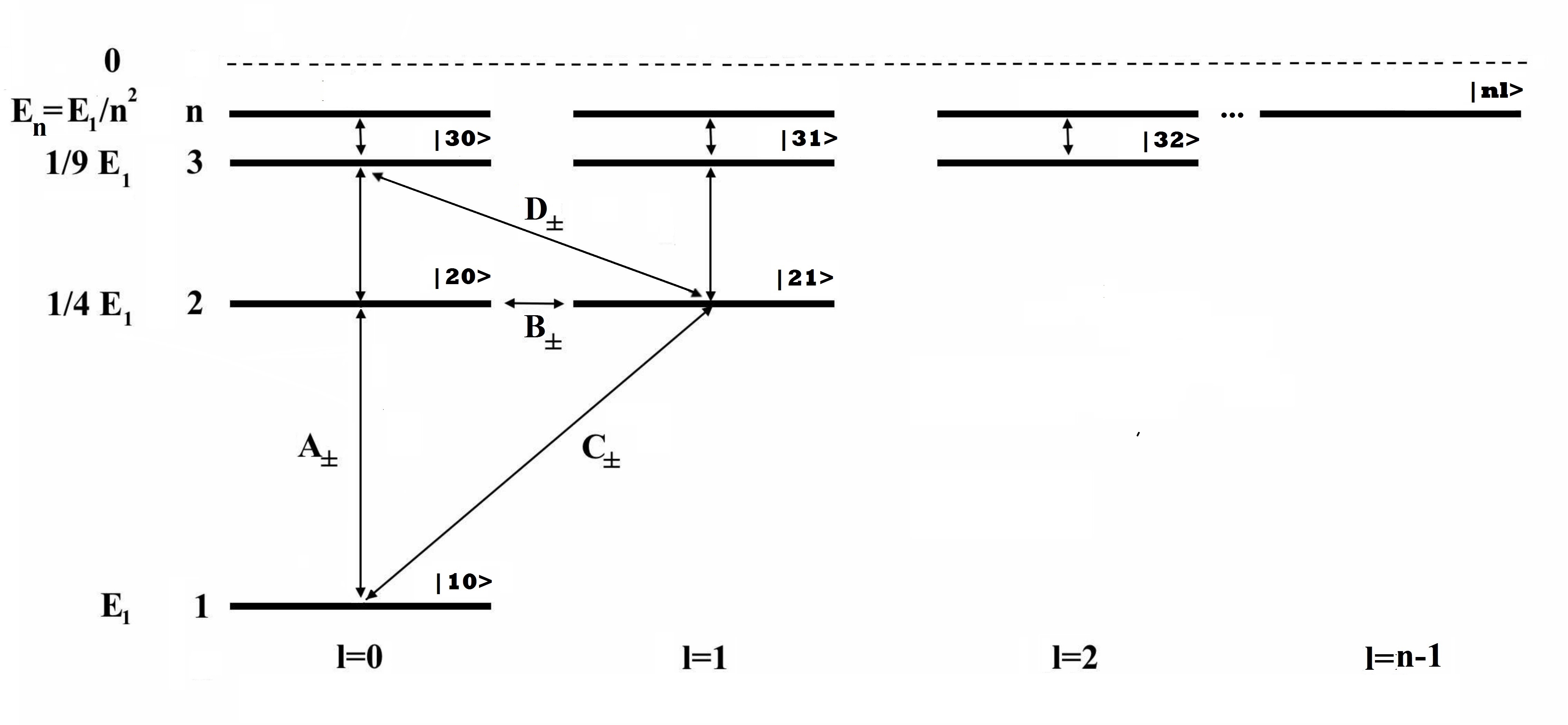
Figure 1: The representation of ladder operators $A_{\pm},B_{\pm},C_{\pm},D_{\pm}$ on the energy levels $\left|{nl}\right\rangle$, $E_{1}\approx-13.6\leavevmode\nobreak\ \rm ev$.

Now, we will detect the radial wave functions $R_{nl}(r)$ related to the HLA as a general formula. The ground states $\phi_{l+1,l}(\rho)$ by substituting $n=l+1$ would be extracted of the following equation:

$$A_{-}\phi_{l+1,l}(\rho)=(-\rho\frac{d}{d\rho}-\frac{\rho}{2}+l)\phi_{l+1,l}(\rho)=0$$ (48)

Based on the normalization relation in Eq. 21, the general solution $\phi_{l+1,l}(\rho)$ is given by:

$$\phi_{l+1,l}(\rho)=\frac{1}{\sqrt{(2l+1)!}}\rho^{l}e^{-\rho/2}$$ (49)

Here, the excited states $\left|{nl}\right\rangle$ will be consecutively ensued from acting the creation operator $A_{+}$ on the ground states $\left|{l+1,l}\right\rangle$ in order of $(n-l-1)$ as a recurrence relation with any constant integer number $l$, in which will be used the eigenvalues $a_{kl}^{+}$ where $k=l+1,l+2,...,n-2,n-1$ as follows:

$${\left|{nl}\right\rangle}=\frac{1}{a^{+}_{n-1,l}a^{+}_{n-2,l}\leavevmode\nobreak\ \cdots a^{+}_{l+1,l}}A_{+}A_{+}\leavevmode\nobreak\ \cdots A_{+}{\left|{l+1,l}\right\rangle}$$

$$=\prod_{k=l+1}^{n-1}\frac{1}{\sqrt{(k-l)(k+l+1)}}A^{n-l-1}_{+}{\left|{l+1,l}\right\rangle}\leavevmode\nobreak\ \leavevmode\nobreak\ \leavevmode\nobreak\ \leavevmode\nobreak\$$ (50)

The solution of the above product converge series reads:

$${\left|{nl}\right\rangle}=\sqrt{\frac{(2l+1)!}{(n+l)!(n-l-1)!}}\leavevmode\nobreak\ A^{n-l-1}_{+}{\left|{l+1,l}\right\rangle}\in L^{2}(\mathbb{R})$$ (51)

In continuation of the discussion, the ahead procedure is an intrinsically interesting result because we don’t need to solve the complicated Laguerre equation. The relationship between the eigenfunctions $\phi_{nl}(\rho)$ and the associated Laguerre’s polynomials meaning that $L_{n+l}^{2l+1}(\rho)$ is [17]:

$$\phi_{nl}(\rho)=-C_{nl}\rho^{l}e^{-\rho/2}L^{2l+1}_{n+l}(\rho)$$ (52)

The Laguerre differential equation is not self-adjoint. As an important result of the Sturm-Liouville theorem and considering appropriate weight factor, the orthonormality condition of the associated Laguerre polynomials is [18, 19]:

$$\int_{0}^{\infty}\rho d\rho\leavevmode\nobreak\ \rho^{2l}e^{-\rho}L^{2l+1}_{\acute{n}+l}(\rho)L^{2l+1}_{n+l}(\rho)=\frac{[(n+l)!]^{3}}{(n-l-1)!}\delta_{\acute{n}n}$$ (53)

Using the normalization condition of $\phi_{nl}(\rho)$, the constant $C_{nl}$ is determined by:

$$\phi_{nl}(\rho)=-{\left[\frac{(n-l-1)!}{[(n+l)!]^{3}}\right]^{\frac{1}{2}}}\rho^{l}e^{-\rho/2}L^{2l+1}_{n+l}(\rho)$$ (54)

Because $R_{nl}(r)=\frac{1}{\sqrt{2n}}\left(\frac{2Z}{na\circ}\right)^{3/2}\phi_{nl}(\rho)$ and $\rho=\frac{2Z}{na_{\circ}}r$, the radial wave functions $R_{nl}(r)$ can be written in the following form:

$$R_{nl}(r)=-{\left(\frac{2Z}{na_{\circ}}\right)^{\frac{3}{2}}}{\left[\frac{(n-l-1)!}{2n[(n+l)!]^{3}}\right]^{\frac{1}{2}}}{\left(\frac{2Z}{na_{\circ}}r\right)^{l}}$$

$$\times L^{2l+1}_{n+l}{\left(\frac{2Z}{na_{\circ}}r\right)}e^{\frac{-Z}{na_{\circ}}r}\leavevmode\nobreak\ \leavevmode\nobreak\ \leavevmode\nobreak\ \leavevmode\nobreak\ \leavevmode\nobreak\ \leavevmode\nobreak\ \leavevmode\nobreak\ \leavevmode\nobreak\ \leavevmode\nobreak\ \leavevmode\nobreak\ \leavevmode\nobreak\ \leavevmode\nobreak\ \leavevmode\nobreak\ \leavevmode\nobreak\ \leavevmode\nobreak\ \leavevmode\nobreak\ \leavevmode\nobreak\ \leavevmode\nobreak\ \leavevmode\nobreak\ \leavevmode\nobreak\$$ (55)

The distribution curve of probability density function $p(r)=r^{2}|R_{nl}(r)|^{2}$ has $(n-l)$ bulges. The expectation value $r^{k}$ which is a special parameter would be achieved as follows [10, 11]:

$${\left\langle r^{k}\right\rangle}_{nl}=\int_{0}^{\infty}dr\leavevmode\nobreak\ r^{2+k}|R_{nl}(r)|^{2}$$ (56)

By the properties of Laguerre polynomials, we show [10]:

$${\left\langle r\right\rangle}_{nl}=\frac{a_{\circ}}{2Z}[3n^{2}-l(l+1)]$$ (57)

$${\left\langle r^{-1}\right\rangle}_{nl}=\frac{Z}{a_{\circ}n^{2}}$$ (58)

According to Bohr’s theory, the maximum Probability of electron presence is in the ground state of $R_{n,n-1}(r)$, where we see the highest bulge. It is $\overline{r}\sim r_{n}=a_{\circ}n^{2}$ as the quantized radius of circular orbits for the Hydrogen atom.
The general eigenstates of the HLA systems, which have a spatial and spin part, are given by:

$$\left|nlm_{l}m_{s}\right\rangle=\left|nlm_{l}\right\rangle\bigotimes\left|s;\leavevmode\nobreak\ m_{s}\right\rangle$$ (59)

The spatial functions $\psi_{nlm_{l}}$ in the spherical coordinate system consist of the radial wave functions $R_{n1}(r)$ and angular dependence $Y_{lm_{l}}(\theta,\varphi)$, which will result in:

$$\psi_{nlm_{l}}(r,\theta,\varphi)=-{\left(\frac{2Z}{na_{\circ}}\right)^{3/2}}{\left[\frac{(n-l-1)!}{2n[(n+l)!]^{3}}\right]^{1/2}}{\left(\frac{2Z}{na_{\circ}}r\right)^{l}}$$

$$\times L^{2l+1}_{n+l}{\left(\frac{2Z}{na_{\circ}}r\right)}e^{-\frac{Z}{na_{\circ}}r}\leavevmode\nobreak\ Y_{lm_{l}}(\theta,\varphi)\leavevmode\nobreak\ \leavevmode\nobreak\ \leavevmode\nobreak\ \leavevmode\nobreak\ \leavevmode\nobreak\ \leavevmode\nobreak\ \leavevmode\nobreak\ \leavevmode\nobreak\$$ (60)

Subsequently, the perfect wave eigenfunctions are:

$$\psi_{nlm_{l}m_{s}}(\overrightarrow{r})=\psi_{nlm_{l}}(r,\theta,\varphi)\left|1/2;\leavevmode\nobreak\ \pm 1/2\right\rangle$$ (61)

These wave functions can be checked in most quantum physics textbooks and other available articles to study more thoroughly.

IV.3 Coherent states

We shall go on to another set of basis states known as the coherent states or Bargmann’s representations, which have far more physical significance than the technical aspects we have already studied. It is only recently that such a concept can be generalized to quantum field theory in depth. The importance of this matter is expanded simultaneously with the fast development of technologies in lasers, photonics science, and quantum optics in recent decades. Not only does the coherent state play a crucial role in new technology, but it also comes with a multitude number of benefits in the future. The coherent states $\left|z\right\rangle$ as either minimum uncertainty states or a set of all eigenvectors of the annihilation operator satisfy the following equation:

$$A_{-}\left|z\right\rangle=z\left|z\right\rangle$$ (62)

They are labeled with the complex numbers $z=|z|e^{iK}$ as general solutions of the eigenvector equation because the operator $A_{-}$ is not a Hermitian operator [20, 21]. By expanding the normalized eigenstates $\left|z\right\rangle$, meaning that $\left\langle z\right|z\rangle=1$ on the standard orthogonal basis $\left|{nl}\right\rangle$ according to the relation $\left|z\right\rangle=\sum_{n}c_{n}\left|{nl}\right\rangle$ and also using Eqs. 22 and 51, we can solve all possible coherent states for any constant integer $l,\leavevmode\nobreak\ n\geq l+1$ as follows:

$$\left|z\right\rangle={M_{l}}\sum_{n}\frac{z^{n-l-1}}{\sqrt{(n+l)!(n-l-1)!}}\left|{nl}\right\rangle$$ (63)

The modified Bessel’s equation of the first kind differs from Bessel ODE but only a small change $x\rightarrow ix$ will be caused to construct the Hyperbolic Bessel functions by an imaginary argument as $I_{l}(x)\equiv e^{-i\pi l/2}J_{l}(ix)=\sum_{k=0}^{\infty}\frac{\left(\frac{x}{2}\right)^{2k+l}}{k!(k+l)!}$ for integer numbers $l,k\geq 0$ and all real values $x\equiv 2|z|\in\mathbb{R}$. The modified functions $I_{l}(x)$ are not oscillatory but have exponential behavior in character (rather than trigonometric). Fortunately, the knowledge that we have developed regarding Bessel ODE can be well used for modified Bessel functions. Here, i t is necessary to note that real recurrence coefficients ${M_{l}}$ are given by [18, 22]:

$${M_{l}}(x)\equiv\left(\frac{x}{2}\right)^{l+1/2}\left[I_{2l+1}(x)\right]^{-1/2}$$

$$=\left[\sum_{k=0}^{\infty}\frac{\left(\frac{x}{2}\right)^{2k}}{k!(k+2l+1)!}\right]^{-1/2}\leavevmode\nobreak\ ,k=0,1,2,...\in\mathbb{Z}$$ (64)

As we all know, the power series expansion of $I_{l}(x),\leavevmode\nobreak\ M_{l}(x)$ is similar to $J_{l}(x)$ but without the alternating factor $(-1)^{m}$.

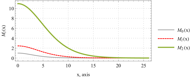
Figure 2: The Bessel’s function of the first kind can be defined by contour’s integral as $J_{l}(x)=\frac{1}{\pi}\int_{0}^{\pi}{d}t\leavevmode\nobreak\ \cos(x\sin t-lt)$ which is valid even for complex arguments meaning that an important special case with a purely imaginary argument $(ix)$. Now, the solutions of Bessel’s equation are called the modified functions (or occasionally the hyperbolic Bessel’s functions).
The functions $J_{l}(ix)$ will be real for all even integers $l$ and take imaginary values for odd integers $l$. To get rid of this simple issue, one introduces into consideration the modified Bessel’s functions $I_{l}(x)=i^{-l}J_{l}(ix)$ which are real for any $l$ and also closely related to $J_{l}(x)$. These entire functions for large values $x$ and integer numbers $l$ can behave similarly to an exponential function of a real positive argument. It is crucial to be noted that unlike the ordinary Bessel’s functions $J_{l}(x)$ which are oscillating, the functions $I_{l}(x)$ and $M_{l}(x)$ are exponentially growing and decaying graphs respectively. we know that the functions $I_{l}(x)$ will go to zero at $x=0$ for $l>{0}$ and are finite at $x=0$ for $l=0$ . The convergent series of $M_{l}(x)$ is primarily involved in a descending sequence as $a_{k}=\frac{1}{4^{k}(k+2l+1)!\leavevmode\nobreak\ k!}$. Since $\lim_{k\to+\infty}|\frac{a_{k+1}}{a_{k}}|=0$, we can find that the rate of convergence with the radius $R=+\infty$ at the infinite interval $-\infty<x<+\infty$ converges to zero super-linearly and very quickly. Here, modified Bessel’s functions $M_{l}(x)$ have been finite at $x>0$ for all $l$ despite a singularity of Gaussian type in very far points but absolutely on the boundary conditions of $x=0$ for any odd integers $l$ are as a one-sided limit.

What truly matters for describing quantum physics is the existence of the completeness relation [21]:

$$\sum_{z}\left|z\right\rangle\left\langle z\right|\equiv\int dz\leavevmode\nobreak\ \left|z\right\rangle\left\langle z\right|=1$$ (65)

The coherent states consist of an overcomplete basis of Hilbert space as can be seen that these elements are never orthogonal, meaning that $\left\langle\acute{z}\right|z\rangle\neq{0}$ [21].

We can rewrite a more convenient expression using Eqs. 51, and 63 as follows:

$$\left|z\right\rangle=D_{l}(z)\left|l+1,l\right\rangle$$ (66)

The displacement operator $D_{l}(z)$ is:

$$D_{l}(z)={M_{l}}{\sqrt{(2l+1)!}}\sum_{K=0}^{\infty}\frac{{z^{k}}}{k!(k+2l+1)!}A_{+}^{K}$$ (67)

By acting $D_{l}(z)$, all normalized coherent states $\left|z\right\rangle$ out of the stationary ground states will be created. It is more interesting that (with the exception $\left|z\right\rangle$ being the vacuum) the coherent states can be projected on any given basis $\left|{nl}\right\rangle$ by:

$$\left\langle nl\right|z\rangle=\frac{{M_{l}}z^{n-l-1}}{\sqrt{(n+l)!(n-l-1)!}}$$ (68)

It contains all possible states of the Fock basis, which are distributed with a Poisson probability distribution.

The probability amplitude of getting the ground state $\left|{10}\right\rangle$ in any coherent state $\left|z\right\rangle$ is:

$$\left\langle 10\right|z\rangle={M_{0}}$$ (69)

On the other hand, the occupation number for the eigenvalues of the Hamiltonian is as random as it can be in any given coherent state through a Poisson distribution [21].

Here, the average value of the occupation number $N$ reads:

$$\overline{N}=|{M_{l}}|^{2}\sum_{k=0}^{\infty}\frac{(k+l+1)}{k!(k+2l+1)!}|z|^{2k}\propto|z|^{2}$$ (70)

Obviously (no matter how small or large), whatever the value of $|z|$ is, the coherent states $\left|z\right\rangle$ constitute a maximally random distribution based on an orthogonal basis, which may predict the important physical attributes.

The following wave functions, normalized to one coherent state, can be computed by:

$$R_{nl}(z,r)={M_{l}}\sum_{n}\frac{z^{n-l-1}}{\sqrt{(n+l)!(n-l-1)!}}R_{nl}(r)$$ (71)

The above-obtained results are explicitly different from the table of coherent states given by approaches such as the group theory. The corresponding coherent states imply that such as aspect can be developed. The annihilation operator will investigate the quantum statistical behavior of the coherent optical fields. We will limit our discussion to a determination of such as initial instructions, while elsewhere, we shall give a more detailed account, including an attempt to obtain more effects. It is more crucial to establish that the coherent state is likewise the smallest deterministic state. Moreover, we will notice shortly that any coherent state is a specific kind of quantum state whose dynamics closely try to simulate the behavior of a classical system.

IV.4 Uncertainty principle

It is necessary to introduce the uncertainty principle after displaying the coherent states. Heisenberg discovered the uncertainty principle in 1926. He observed that every pair of non-commuting physical properties may result in an uncertainty relationship. Such an assumption led to the development of quantum mechanics theory. We have a system with appropriately normalized wave functions and ladder operators $A_{\pm}$ that:

$$A_{\pm}=\frac{1}{\sqrt{2}}(q\mp ip)$$ (72)

The uncertainty in two Hermitian dimensionless operators $q,p$ will be defined by taking into consideration $\sigma_{q}\equiv\Delta q$ and $\sigma_{p}\equiv\Delta p$ as follows:

$$\sigma_{q}\sigma_{p}\geq\frac{1}{2}|\left\langle[q,p]\right\rangle|$$ (73)

This matter is called Heisenberg’s uncertainty principle.

Using Eqs. 45 and 72, since $[A_{-},A_{+}]=\frac{1}{i}[q,p]=2N$, and the operators $q,p$ are symmetric, the uncertainty relationship can be applied to them:

$$\sigma_{q}\sigma_{p}\geq\overline{N}$$ (74)

Based on the expectation value of occupation number $N$, the indeterminacy is related to complex variables $z$ and the quantum numbers $n,l$. Our primary goal is to find the wave functions known as the least indeterminacy states that satisfy Heisenberg’s uncertainty principle with equality.

By considering Eqs. 45, 62, and 72, the uncertainty of the symmetric operators $q,p$ in the state $\left|z\right\rangle$ reads:

$$\left(\Delta q\right)^{2}_{z}\equiv{\left\langle q^{2}\right\rangle}_{z}-{\left\langle q\right\rangle}_{z}^{2}=\overline{N}$$ (75)

$$\left(\Delta p\right)^{2}_{z}\equiv{\left\langle p^{2}\right\rangle}_{z}-{\left\langle p\right\rangle}_{z}^{2}=\overline{N}$$ (76)

We get the uncertainty relationship with equality by using Eqs. 75 and 76, which follows:

$$\left(\sigma_{q}\right)_{z}\left(\sigma_{p}\right)_{z}=\overline{N}$$ (77)

The equal sign implies in the preceding formula that the coherent states $\left|z\right\rangle$ are the least indeterminacy states and $R_{nl}(z,r)$ are the minimum uncertainty wave functions. We can also apply the uncertainty principle on the basis $\left|{nl}\right\rangle$ by Eqs.28 and 74 as follows:

$$\left(\sigma_{q}\right)_{nl}\left(\sigma_{p}\right)_{nl}\geq n$$ (78)

Besides, in a similar way by computing all expectation values, the uncertainty of the symmetric operators $q,p$ in the basis state $\left|{nl}\right\rangle$ is:

$$\left(\sigma_{q}\right)_{nl}\left(\sigma_{p}\right)_{nl}=n^{2}-l(l+1),\leavevmode\nobreak\ n\geq{l+1}$$ (79)

Hence, the inequality of Eq. 78 will be easily extracted as a result of assumption $n^{2}-l(l+1)\geq n$. The important point that would be cause all wave functions $\left|{nl}\right\rangle,\leavevmode\nobreak\ n\neq l+1$ to have no the minimal indeterminacy is that $A_{-}\left|{nl}\right\rangle\neq 0$. We know that $\left|{nl}\right\rangle$ is not an eigenstate of the operator $A_{-}$ and it has a non-minimum uncertainty since the uncertainty grows with all values $n\neq l+1$.

Where the wave functions are orthonormal, the equation $A_{-}\left|{l+1,l}\right\rangle=0,\leavevmode\nobreak\ n=l+1$ can lead to:

$$\left(\sigma_{q}\right)_{l+1,l}\left(\sigma_{p}\right)_{l+1,l}=l+1$$ (80)

The comparison of Eqs. 78 and 80 plainly expresses that the ground state $\left|{l+1,l}\right\rangle$ is a minimum uncertainty wave function for any constant value $l$. We can also expect other minimum uncertainty function $\left|z\right\rangle$ due to satisfying the relationship $A_{-}\left|z\right\rangle=z\left|z\right\rangle$.

V Conclusion

The energy quantization and wave functions have been extracted for the HLA quantum systems by the creation and annihilation operators in Hilbert space without any arbitrary assumptions. The radius and transition relations literally can obtain not using the analytical solution of Schrödinger’s equation. It is necessary to consider a few corrections in a much more realistic study of Hydrogen atom, such as one of the most important cases is the relativistic motion of electrons which has caused the emergence of terms in the kinetic energy and We should solve it by the perturbation theory. Incidentally, another correction from a large order of reduced mass will be related to interaction of the nucleus electromagnetic field with the electron spin. We hope with an emphasis on research with lasting and profound impact to see more empirical applications of the algebraic method by making an appropriate groundwork to discover the coherent states of Hydrogen atom in the quantum field theory (QFT) and elsewhere. Moreover, it is a brilliant way to produce new technology.

Appendix A: Matrix representations of introduced operators in the N-space

The matrix representation $N,H_{N}$ for the column $l=0$ in the basis $\left|nl\right\rangle$ is:

$$N=\begin{pmatrix}1&0&0&\cdots\\ 0&2&0&\cdots\\ 0&0&3&\cdots\\ \vdots&\vdots&\vdots&\ddots\end{pmatrix},\leavevmode\nobreak\ \leavevmode\nobreak\ H_{N}=\begin{pmatrix}{\left\langle 10\right|H_{N}}{\left|10\right\rangle}&{\left\langle 10\right|H_{N}}{\left|20\right\rangle}&{\left\langle 10\right|H_{N}}{\left|30\right\rangle}&\cdots\\ {\left\langle 20\right|H_{N}}{\left|10\right\rangle}&{\left\langle 20\right|H_{N}}{\left|20\right\rangle}&{\left\langle 20\right|H_{N}}{\left|30\right\rangle}&\cdots\\ {\left\langle 30\right|H_{N}}{\left|10\right\rangle}&{\left\langle 30\right|H_{N}}{\left|20\right\rangle}&{\left\langle 30\right|H_{N}}{\left|30\right\rangle}&\cdots\\ \vdots&\vdots&\vdots&\ddots\end{pmatrix}=\begin{pmatrix}0&0&0&\cdots\\ 0&0&0&\cdots\\ 0&0&0&\cdots\\ \vdots&\vdots&\vdots&\ddots\end{pmatrix}$$ (81)

The matrix representation of the vertical ladder operators $A_{\pm}$ is:

$$A_{+}=\begin{pmatrix}0&0&0&0&\cdots\\ \sqrt{2}&0&0&0&\cdots\\ 0&\sqrt{6}&0&0&\cdots\\ 0&0&2\sqrt{3}&0&\cdots\\ \vdots&\vdots&\vdots&\vdots&\ddots\end{pmatrix},\leavevmode\nobreak\ \leavevmode\nobreak\ A_{-}=\begin{pmatrix}0&\sqrt{2}&0&0&\cdots\\ 0&0&\sqrt{6}&0&\cdots\\ 0&0&0&2\sqrt{3}&\cdots\\ 0&0&0&0&\cdots\\ \vdots&\vdots&\vdots&\vdots&\ddots\end{pmatrix}$$ (82)

The joint eigenvectors of $N,H_{N}$ can be obtained according to Eq. 28 as follows:

$$N\left|{nl}\right\rangle=\begin{pmatrix}1&0&0&\cdots\\ 0&2&0&\cdots\\ 0&0&3&\cdots\\ \vdots&\vdots&\vdots&\ddots\end{pmatrix}\begin{pmatrix}a\\ b\\ c\\ \vdots\end{pmatrix}=n\begin{pmatrix}a\\ b\\ c\\ \vdots\end{pmatrix}\Rightarrow\begin{cases}\leavevmode\nobreak\ a=na\\ \leavevmode\nobreak\ 2b=nb\\ \leavevmode\nobreak\ 3c=nc\\ \leavevmode\nobreak\ \vdots\end{cases}$$ (83)

The normalized solutions of these equations for $n=1,2,3,...\in\mathbb{N}$ are respectively given by:

$$\left|10\right\rangle=\begin{pmatrix}1\\ 0\\ 0\\ \vdots\end{pmatrix},\leavevmode\nobreak\ \left|20\right\rangle=\begin{pmatrix}0\\ 1\\ 0\\ \vdots\end{pmatrix},\leavevmode\nobreak\ \left|30\right\rangle=\begin{pmatrix}0\\ 0\\ 1\\ \vdots\end{pmatrix},...$$ (84)

We can verify that these vectors are orthonormal. Hence according to Eq. 22, it is easy to see that:

$$\left\langle\acute{n},0|n,0\right\rangle=\delta_{\acute{n}n}$$ (85)

We can also verify that they are complete. Hence according to Eq. 22, we have:

$$\sum_{n=1}^{N}\left|n,0\right\rangle\left\langle n,0\right|=\begin{pmatrix}1\\ 0\\ 0\\ \vdots\end{pmatrix}\begin{pmatrix}1&0&0&\cdots\end{pmatrix}+\begin{pmatrix}0\\ 1\\ 0\\ \vdots\end{pmatrix}\begin{pmatrix}0&1&0&\cdots\end{pmatrix}+\begin{pmatrix}0\\ 0\\ 1\\ \vdots\end{pmatrix}\begin{pmatrix}0&0&1&\cdots\end{pmatrix}+...=\begin{pmatrix}1&0&0&\cdots\\ 0&1&0&\cdots\\ 0&0&1&\cdots\\ \vdots&\vdots&\vdots&\ddots\end{pmatrix}\Rightarrow$$

$$\sum_{n=1}^{N}\left|n,0\right\rangle\left\langle n,0\right|=1$$ (86)

The position and radial momentum operators $\rho,P_{\rho}$ in terms of $A_{\pm}$ using Eq. 27 are given by:

$$\rho=2N-(A_{-}+A_{+})$$ (87)

$$P_{\rho}=\frac{i\hbar}{2}\rho^{-1}(A_{-}-A_{+})$$ (88)

The matrix representation of these operators is:

$$P_{\rho}=\frac{i\hbar}{2}\begin{pmatrix}-3/5&2\sqrt{2}/5&2\sqrt{3}/5&\cdots\\ -3\sqrt{2}/5&1/5&2\sqrt{6}/5&\cdots\\ -4\sqrt{3}/15&-4\sqrt{6}/15&1/5&\cdots\\ \vdots&\vdots&\vdots&\ddots\end{pmatrix},\leavevmode\nobreak\ \leavevmode\nobreak\ \rho=\begin{pmatrix}2&-\sqrt{2}&0&0&\cdots\\ -\sqrt{2}&4&-\sqrt{6}&0&\cdots\\ 0&-\sqrt{6}&6&-2\sqrt{3}&\cdots\\ 0&0&-2\sqrt{3}&8&\cdots\\ \vdots&\vdots&\vdots&\vdots&\ddots\end{pmatrix}$$ (89)

It is important to be noted that the matrix representation of the operator $\rho P_{\rho}$ is:

$$\rho P_{\rho}=\frac{i\hbar}{2}\begin{pmatrix}0&\sqrt{2}&0&0&\cdots\\ -\sqrt{2}&0&\sqrt{6}&0&\cdots\\ 0&-\sqrt{6}&0&2\sqrt{3}&\cdots\\ 0&0&-2\sqrt{3}&0&\cdots\\ \vdots&\vdots&\vdots&\vdots&\ddots\end{pmatrix}$$ (90)

Since the expectation values of $\left\{A_{\pm}^{2},A_{\pm},\rho P_{\rho}\right\}$ in the basis $\left|nl\right\rangle$ are zero and also $\left\langle\rho\right\rangle_{nl}=2n$ then:

$${\left\langle\rho^{2}\right\rangle}_{nl}=6n^{2}-2l(l+1)$$ (91)

$${\left\langle\rho^{2}P_{\rho}^{2}\right\rangle}_{nl}=\frac{\hbar^{2}}{2}\left[n^{2}-l(l+1)\right]$$ (92)

The expectation value $H_{N}$ in the basis $\left|nl\right\rangle$ based on Eq. 29 reads:

$$\overline{H}_{N}=l(l+1)$$ (93)

We can calculate ${\left\langle(\Delta A)^{2}\right\rangle}{\left\langle(\Delta B)^{2}\right\rangle}\geq\frac{1}{4}|{\left\langle[A,B]\right\rangle}|^{2}$ according to $[\rho,P_{\rho}]=i\hbar$, hence:

$$\Delta\rho\Delta P_{\rho}\geq\frac{\hbar}{2}$$ (94)

What equally matters based on Heisenberg’s principle for quantum physics is minimizing the uncertainty distributed in both symmetric operators.
The matrix representation $N,H_{N}$ for the column $l=1$ in the basis $\left|nl\right\rangle$ is:

$$N=\begin{pmatrix}2&0&0&\cdots\\ 0&3&0&\cdots\\ 0&0&4&\cdots\\ \vdots&\vdots&\vdots&\ddots\end{pmatrix},\leavevmode\nobreak\ H_{N}=\begin{pmatrix}{\left\langle 21\right|H_{N}}{\left|21\right\rangle}&{\left\langle 21\right|H_{N}}{\left|31\right\rangle}&{\left\langle 21\right|H_{N}}{\left|41\right\rangle}&\cdots\\ {\left\langle 31\right|H_{N}}{\left|21\right\rangle}&{\left\langle 31\right|H_{N}}{\left|31\right\rangle}&{\left\langle 31\right|H_{N}}{\left|41\right\rangle}&\cdots\\ {\left\langle 41\right|H_{N}}{\left|21\right\rangle}&{\left\langle 41\right|H_{N}}{\left|31\right\rangle}&{\left\langle 41\right|H_{N}}{\left|41\right\rangle}&\cdots\\ \vdots&\vdots&\vdots&\ddots\end{pmatrix}=2\begin{pmatrix}1&0&0&\cdots\\ 0&1&0&\cdots\\ 0&0&1&\cdots\\ \vdots&\vdots&\vdots&\ddots\end{pmatrix}$$ (95)

The matrix representation of the vertical ladder operators $A_{\pm}$ and $\rho$ is:

$$A_{+}=\begin{pmatrix}0&0&0&0&\cdots\\ 2&0&0&0&\cdots\\ 0&\sqrt{10}&0&0&\cdots\\ 0&0&3\sqrt{2}&0&\cdots\\ \vdots&\vdots&\vdots&\vdots&\ddots\end{pmatrix},\leavevmode\nobreak\ A_{-}=\begin{pmatrix}0&2&0&0&\cdots\\ 0&0&\sqrt{10}&0&\cdots\\ 0&0&0&3\sqrt{2}&\cdots\\ 0&0&0&0&\cdots\\ \vdots&\vdots&\vdots&\vdots&\ddots\end{pmatrix},\leavevmode\nobreak\ \rho=\begin{pmatrix}4&-2&0&\cdots\\ -2&6&-\sqrt{10}&\cdots\\ 0&-\sqrt{10}&8&\cdots\\ \vdots&\vdots&\vdots&\ddots\end{pmatrix}$$ (96)

It is quite clear that the matrix representation of the operators $P_{\rho},\rho P_{\rho}$ is:

$$P_{\rho}=\frac{i\hbar}{2}\begin{pmatrix}-31/105&43/105&11\sqrt{10}/105&\cdots\\ -62/105&-19/105&22\sqrt{10}/105&\cdots\\ -2\sqrt{10}/21&-4\sqrt{10}/21&1/21&\cdots\\ \vdots&\vdots&\vdots&\ddots\end{pmatrix},\leavevmode\nobreak\ \leavevmode\nobreak\ \rho P_{\rho}=\frac{i\hbar}{2}\begin{pmatrix}0&2&0&0&\cdots\\ -2&0&\sqrt{10}&0&\cdots\\ 0&-\sqrt{10}&0&3\sqrt{2}&\cdots\\ 0&0&-3\sqrt{2}&0&\cdots\\ \vdots&\vdots&\vdots&\vdots&\ddots\end{pmatrix}$$ (97)

The joint eigenvectors of $N,H_{N}$ can be obtained according to Eq. 28 as follows:

$$N\left|{nl}\right\rangle=\begin{pmatrix}2&0&0&\cdots\\ 0&3&0&\cdots\\ 0&0&4&\cdots\\ \vdots&\vdots&\vdots&\ddots\end{pmatrix}\begin{pmatrix}a\\ b\\ c\\ \vdots\end{pmatrix}=n\begin{pmatrix}a\\ b\\ c\\ \vdots\end{pmatrix}\Rightarrow\begin{cases}\leavevmode\nobreak\ 2a=na\\ \leavevmode\nobreak\ 3b=nb\\ \leavevmode\nobreak\ 4c=nc\\ \leavevmode\nobreak\ \vdots\end{cases}$$ (98)

The normalized solutions of these equations for $n=2,3,4,...\in\mathbb{N}$ are respectively given by:

$$\left|21\right\rangle=\begin{pmatrix}1\\ 0\\ 0\\ \vdots\end{pmatrix},\leavevmode\nobreak\ \left|31\right\rangle=\begin{pmatrix}0\\ 1\\ 0\\ \vdots\end{pmatrix},\leavevmode\nobreak\ \left|41\right\rangle=\begin{pmatrix}0\\ 0\\ 1\\ \vdots\end{pmatrix},...$$ (99)

We can verify that these vectors are orthonormal, and according to Eq. 22, we have:

$$\left\langle\acute{n},1|n,1\right\rangle=\delta_{\acute{n}n},\leavevmode\nobreak\ \sum_{n=2}^{N}\left|n,1\right\rangle\left\langle n,1\right|=1$$ (100)

Appendix B: Some arbitrary points of the first modified functions ${M_{l}}$

$x$	$M_{0}$	$M_{1}$	$M_{2}$	$M_{3}$	$M_{4}$	$M_{5}$
0.0	1.0000000000	2.4494897428	10.9544511501	70.9929573972	602.3952191045	6317.9743589223
0.1	0.9993753253	2.4487244447	10.9521692784	70.9818658067	602.3199252637	6317.3162761421
0.2	0.9975051971	2.4464305576	10.9453273289	70.9486037406	602.0941104643	6315.3425022980
0.3	0.9944012393	2.4426140912	10.9339362860	70.8932092849	601.7179747578	6312.0544602172
0.4	0.9900826177	2.4372850211	10.9180144144	70.8157458168	601.1918511720	6307.4545190678
0.5	0.9845757344	2.4304572283	10.8975871963	70.7163018552	600.5162051248	6301.5459910489
0.6	0.9779138150	2.4221484155	10.8726872434	70.5949908532	599.6916336058	6294.3331267679
0.7	0.9701363985	2.4123800015	10.8433541846	70.4519509323	598.7188641290	6285.8211093137
0.8	0.9612887480	2.4011769941	10.8096345309	70.2873445593	597.5987534583	6276.0160470419
0.9	0.9514211956	2.3885678432	10.7715815165	70.1013581684	596.3322861106	6264.9249650860
1.0	0.9405884429	2.3745842767	10.7292549197	69.8942017288	594.9205726399	6252.5557956163
1.1	0.9288488317	2.3592611192	10.6827208616	69.6661082602	593.3648477092	6238.9173668661
1.2	0.9162636050	2.3426360964	10.6320515865	69.4173332973	591.6664679529	6224.0193909517
1.3	0.9028961733	2.3247496277	10.5773252239	69.1481543072	589.8269096393	6207.8724505135
1.4	0.8888114010	2.3056446078	10.5186255334	68.8588700592	587.8477661365	6190.4879842073
1.5	0.8740749261	2.2853661803	10.4560416350	68.5497999524	585.7307451919	6171.8782710784
1.6	0.8587525237	2.2639615049	10.3896677245	68.2212833017	583.4776660309	6152.0564138539
1.7	0.8429095207	2.2414795214	10.3196027783	67.8736785851	581.0904562840	6131.0363211899
1.8	0.8266102686	2.2179707104	10.2459502459	67.5073626562	578.5711487508	6108.8326889116
1.9	0.8099176768	2.1934868549	10.1688177348	67.1227299240	575.9218780094	6085.4609802887
2.0	0.7928928100	2.1680808035	10.0883166874	66.7201915024	573.1448768809	6060.9374053879
2.1	0.7755945465	2.1418062367	10.0045620520	66.3001743343	570.2424727586	6035.2788995481
2.2	0.7580792996	2.1147174388	09.9176719502	65.8631202913	567.2170838117	6008.5031010223
2.3	0.7404007957	2.0868690762	09.8277673421	65.4094852536	564.0712150734	5980.6283278365
2.4	0.7226099073	2.0583159835	09.7349716890	64.9397381725	560.8074544237	5951.6735539115
2.5	0.7047545368	2.0291129592	09.6394106188	64.4543601195	557.4284684786	5921.6583844998
2.6	0.6868795446	1.9993145702	09.5412115916	63.9538433234	553.9369983934	5890.6030309864
2.7	0.6690267182	1.9689749685	09.4405035698	63.4386902007	550.3358555938	5858.5282851066
2.8	0.6512347755	1.9381477185	09.3374166922	62.9094123809	546.6279174439	5825.4554926318
2.9	0.6335393998	1.9068856365	09.2320819546	62.3665297296	542.8161228612	5791.4065265777
3.0	0.6159732983	1.8752406425	09.1246308968	61.8105693736	538.9034678908	5756.4037599850
3.1	0.5985662837	1.8432636247	09.0151952982	61.2420647297	534.8930012477	5720.4700383298
3.2	0.5813453711	1.8110043165	08.9039068825	60.6615545397	530.7878198385	5683.6286516137
3.3	0.5643348888	1.7785111855	08.7908970320	60.0695819156	526.5910642729	5645.9033061881
3.4	0.5475565993	1.7458313364	08.6762965128	59.4666933962	522.3059143739	5607.3180963658
3.5	0.5310298264	1.7130104242	08.5602352117	58.8534380186	517.9355846977	5567.8974758725
3.6	0.5147715879	1.6800925806	08.4428418844	58.2303664052	513.4833200724	5527.6662291893
3.7	0.4987967293	1.6471203515	08.3242439171	57.5980298707	508.9523911648	5486.6494428387
3.8	0.4831180593	1.6141346451	08.2045671003	56.9569795490	504.3460900844	5444.8724766648
3.9	0.4677464831	1.5811746910	08.0839354160	56.3077655428	499.6677260332	5402.3609351557
4.0	0.4526911341	1.5482780089	07.9624708387	55.6509360977	494.9206210098	5359.1406388593
4.1	0.4379595018	1.5154803868	07.8402931497	54.9870368021	490.1081055758	5315.2375959378
4.2	0.4235575563	1.4828158678	07.7175197649	54.3166098142	485.2335146919	5270.6779739097
4.3	0.4094898668	1.4503167453	07.5942655769	53.6401931176	480.3001836315	5225.4880716215
4.4	0.3957597168	1.4180135656	07.4706428102	52.9583198068	475.3114439775	5179.6942914951
4.5	0.3823692120	1.3859351370	07.3467608903	52.2715174027	470.2706197104	5133.3231120923
4.6	0.3693193842	1.3541085461	07.2227263254	51.5803072006	465.1810233922	5086.4010610367
4.7	0.3566102881	1.3225591787	07.0986426025	50.8852036489	460.0459524526	5038.9546883320
4.8	0.3442410937	1.2913107472	06.9746100948	50.1867137617	454.8686855820	4991.0105401148
4.9	0.3322101723	1.2603853208	06.8507259825	49.4853365642	449.6524792366	4942.5951328764
5.0	0.3205151771	1.2298033617	06.7270841858	48.7815625708	444.4005642600	4893.7349281876

Table 1: The values called from the graphs of modified Bessel’s functions-orders 0,1,2,3,4 and 5 of ${M_{l}}(x)=\left(\frac{x}{2}\right)^{l+1/2}\left[I_{2l+1}(x)\right]^{-1/2}$ are determined with extra precision of $10^{-10}$. While naturally because of singularity at $x=0$, these estimated values measure as a one-sided limit.

Appendix C: Computing the first radial wave functions $R_{nl}(r)$

We will extract the wave functions related to the ground state $\left|10\right\rangle$. Based on Eq. 47, and the normalization condition of Eq. 21, the annihilation operator $A_{-}$ can generate the following results:

$$A_{-}\phi_{10}(\rho)=\left(-\rho\frac{d}{d\rho}-\frac{\rho}{2}\right)\phi_{10}(\rho)=0\$$ (101)

Where $\phi_{10}(\rho)=e^{-\rho/2}$, and since $R_{10}(r)=\frac{1}{\sqrt{2}}\left(\frac{2Z}{a_{\circ}}\right)^{3/2}\phi_{10}(\rho),\leavevmode\nobreak\ \rho=\frac{2Z}{a_{\circ}}r$ then:

$$R_{10}(r)=2\left(\frac{Z}{a_{\circ}}\right)^{3/2}e^{-\frac{Z}{a_{\circ}}r}$$ (102)

By acting the creation operator $A_{+}$ on $\phi_{10}(\rho)$, we can say that:

$$A_{+}\phi_{10}(\rho)=\left(\rho\frac{d}{d\rho}-\frac{\rho}{2}+2\right)\phi_{10}(\rho)=\sqrt{2}\phi_{20}(\rho)$$ (103)

Where $\phi_{20}(\rho)=\frac{1}{\sqrt{2}}(2-\rho)e^{-\rho/2}$ and since $R_{20}(r)=\frac{1}{2}\left(\frac{Z}{a_{\circ}}\right)^{3/2}\phi_{20}(\rho),\leavevmode\nobreak\ \rho=\frac{Z}{a_{\circ}}r$ then:

$$R_{20}(r)=2\left(\frac{Z}{2a_{\circ}}\right)^{3/2}\left(1-\frac{Z}{2a_{\circ}}r\right)e^{-\frac{Z}{2a_{\circ}}r}$$ (104)

By acting the creation operator $A_{+}$ on $\phi_{20}(\rho),$ it is obvious that:

$$A_{+}\phi_{20}(\rho)=\left(\rho\frac{d}{d\rho}-\frac{\rho}{2}+3\right)\phi_{20}(\rho)=\sqrt{6}\phi_{30}(\rho)$$ (105)

Where $\phi_{30}(\rho)=\frac{1}{\sqrt{3}}\left(3-3\rho+\frac{\rho^{2}}{2}\right)e^{-\rho/2}$, and since $R_{30}(r)=\frac{1}{\sqrt{6}}\left(\frac{2Z}{3a_{\circ}}\right)^{3/2}\phi_{30}(\rho),\leavevmode\nobreak\ \rho=\frac{2Z}{3a_{\circ}}r$ then:

$$R_{30}(r)=2\left(\frac{Z}{3a_{\circ}}\right)^{3/2}\left[1-\frac{2Z}{3a_{\circ}}r+\frac{2}{27}\left(\frac{Z}{a_{\circ}}\right)^{2}r^{2}\right]e^{-\frac{Z}{3a_{\circ}}r}$$ (106)

Hence, the radial wave functions $R_{10}(r),R_{20}(r),R_{30}(r)$ are obtained.

We will extract the radial wave functions related to the ground state $\left|21\right\rangle$ that by the annihilation operator $A_{-}$ and using the normalization condition, we have:

$$A_{-}\phi_{21}(\rho)=\left(-\rho\frac{d}{d\rho}-\frac{\rho}{2}+1\right)\phi_{21}(\rho)=0$$ (107)

Where $\phi_{21}(\rho)=\frac{1}{\sqrt{6}}\rho e^{-\rho/2}$, and since $R_{21}(r)=\frac{1}{2}\left(\frac{Z}{a_{\circ}}\right)^{3/2}\phi_{21}(\rho),\leavevmode\nobreak\ \rho=\frac{Z}{a_{\circ}}r$ then:

$$R_{21}(r)=\frac{1}{\sqrt{3}}\left(\frac{Z}{2a_{\circ}}\right)^{3/2}\left(\frac{Z}{a_{\circ}}r\right)e^{-\frac{Z}{2a_{\circ}}r}$$ (108)

By acting the creation operator $A_{+}$ on $\phi_{21}(\rho),$ the following result reads:

$$A_{+}\phi_{21}(\rho)=\left(\rho\frac{d}{d\rho}-\frac{\rho}{2}+3\right)\phi_{21}(\rho)=2\phi_{31}(\rho)$$ (109)

Where $\phi_{31}(\rho)=\frac{1}{2\sqrt{6}}\rho(4-\rho)e^{-\rho/2}$, and since $R_{31}(r)=\frac{1}{\sqrt{6}}\left(\frac{2Z}{3a_{\circ}}\right)^{3/2}\phi_{31}(\rho),\leavevmode\nobreak\ \rho=\frac{2Z}{3a_{\circ}}r$ then:

$$R_{31}(r)=\frac{4\sqrt{2}}{9}\left(\frac{Z}{3a_{\circ}}\right)^{3/2}\left(\frac{Z}{a_{\circ}}r\right)\left(1-\frac{Z}{6a_{\circ}}r\right)e^{-\frac{Z}{3a_{\circ}}r}$$ (110)

Hence, the radial wave functions $R_{21}(r),R_{31}(r)$ are obtained.

We can extract the radial wave function related to the ground state $\left|32\right\rangle$ that using the annihilation operator $A_{-}$ and the normalization condition is given by:

$$A_{-}\phi_{32}(\rho)=\left(-\rho\frac{d}{d\rho}-\frac{\rho}{2}+2\right)\phi_{32}(\rho)=0$$ (111)

Where $\phi_{32}(\rho)=\frac{1}{2\sqrt{30}}\rho^{2}e^{-\rho/2}$, and since $R_{32}(r)=\frac{1}{\sqrt{6}}\left(\frac{2Z}{3a_{\circ}}\right)^{3/2}\phi_{32}(\rho),\leavevmode\nobreak\ \rho=\frac{2Z}{3a_{\circ}}r$ then:

$$R_{32}(r)=\frac{2\sqrt{2}}{27\sqrt{5}}\left(\frac{Z}{3a_{\circ}}\right)^{3/2}\left(\frac{Z}{a_{\circ}}r\right)^{2}e^{-\frac{Z}{3a_{\circ}}r}$$ (112)

Hence, the radial wave function $R_{32}(r)$ is obtained.

References

- Martínez-y-Romero et al. [2007] R. P. Martínez-y-Romero, H. N. Núñez-Yépez, and A. L. Salas-Brito, An operator solution for the hydrogen atom using the phase as an additional variable, American Journal of Physics 75, 629 (2007).
- Martínez-Y-Romero et al. [2007] R. P. Martínez-Y-Romero, H. N. Núñez-Yépez, and A. L. Salas-Brito, Algebraic approach to radial ladder operators in the hydrogen atom, International Journal of Quantum Chemistry 107, 1608 (2007).
- Liu et al. [1997] Y. F. Liu, Y. A. Lei, and J. Y. Zeng, Factorization of the radial Schrödinger equation and four kinds of raising and lowering operators of hydrogen atoms and isotropic harmonic oscillators, Physics Letters A 231, 9 (1997).
- de la Peña and Montemayor [1980] L. de la Peña and R. Montemayor, Raising and lowering operators and spectral structure: A concise algebraic technique, American Journal of Physics 48, 855 (1980).
- Zhi-xiang [1999] N. Zhi-xiang, Vector ladder operators for the central potentials, Acta Physica Sinica 8, 8-13 (1999).
- Joshi [2018] A. W. Joshi, Elements of Group Theory for Physicists (New Age International, New York, 2018).
- Wigner and Massey [2013] E. Wigner and H. Massey, Group Theory: And Its Application to the Quantum Mechanics of Atomic Spectra (Elsevier Science, 2013).
- Pauli [1926] W. Pauli, Über das Wasserstoffspektrum vom Standpunkt der neuen Quantenmechanik, Zeitschrift fur Physik 36, 336 (1926).
- Gerry [1984] C. C. Gerry, On coherent states for the hydrogen atom, Journal of Physics A Mathematical General 17, L737 (1984).
- Zettili [2009] N. Zettili, Quantum Mechanics: Concepts and Applications (Wiley, 2009).
- Gasiorowicz [2007] S. Gasiorowicz, Quantum Physics, 3Rd Ed (Wiley India Pvt. Limited, 2007).
- Sakurai and Napolitano [2020] J. Sakurai and J. Napolitano, Modern Quantum Mechanics (Cambridge University Press, 2020).
- Weidner and Sells [1980] R. Weidner and R. Sells, Elementary Modern Physics, College physics series (Allyn and Bacon, 1980).
- Prugovecki [2013] E. Prugovecki, Quantum Mechanics in Hilbert Space: Second Edition, Dover Books on Physics (Academic press, New York, 2013).
- Xu and Kong [1999] B.-W. Xu and F.-M. Kong, Factorization of the radial Schrödinger equation of the hydrogen atom, Physics Letters A 259, 212 (1999).
- De Lange et al. [1991] O. De Lange, R. Raab, and B. Raab, Operator Methods in Quantum Mechanics, Oxford science publications (Clarendon Press, 1991).
- Pauling and Wilson [2012] L. Pauling and E. Wilson, Introduction to Quantum Mechanics with Applications to Chemistry, Dover Books on Physics (McGraw-Hill Book Co., New York, 2012).
- Arfken et al. [2013] G. Arfken, H. Weber, and F. Harris, Mathematical Methods for Physicists: A Comprehensive Guide (Academic Press, Elsevier Science, 2013).
- Boas [2006] M. Boas, Mathematical Methods in the Physical Sciences (Wiley, 2006).
- Glauber [1963] R. J. Glauber, Coherent and Incoherent States of the Radiation Field, Physical Review 131, 2766 (1963).
- Baulieu et al. [2017] L. Baulieu, J. Iliopoulos, R. Seneor, and R. Sénéor, From Classical to Quantum Fields (Oxford Press, 2017).
- Korenev [2019] B. Korenev, Bessel Functions and Their Applications (Taylor & Francis Group, 2019).