Gravitational collapse in generalized K-essence emergent Vaidya spacetime via $f(\bar{R},\bar{T})$ gravity

Abstract

This study focuses on investigating the collapse possibilities of the generalized emergent Vaidya spacetime within the framework of $f(\bar{R},\bar{T})$ gravity, specifically in the setting of K-essence theory. The Dirac-Born-Infeld type non-standard Lagrangian is used in this work to determine the emergent metric $\bar{G}_{\mu\nu}$, which is not conformally equal to the usual gravitational metric. Here, we employ the function $f(\bar{R},\bar{T})$ to represent the additive character of the emergent Ricci scalar ($\bar{R}$) and trace of the emergent energy-momentum tensor ($\bar{T}$). In our analysis, it can be shown that certain selections of $f(\bar{R},\bar{T})$ can lead to the presence of a naked singularity resulting from gravitational collapse. Additionally, alternative choices of $f(\bar{R},\bar{T})$ were found to yield an accelerating universe primarily governed by dark energy. In addition, the investigation revealed the existence of both positive and negative masses, which can be understood as a gravitational dipole. It is also found that the K-essence theory has the potential to serve as both a dark energy framework and a simple gravitational theory at the same time, allowing for the investigation of a wide range of cosmological phenomena.

I Introduction

Gravitational collapse is a well-recognised phenomenon in the fields of general relativity and astrophysics, as evidenced by the works of Joshi et al. [1, 2]. It serves as a crucial avenue for comprehending many astrophysical facets inside our universe. The phenomenon of gravitational collapse offers valuable insights into several aspects of astrophysics, such as structure development, stellar characteristics, black hole generation, and the formation of white dwarfs or neutron stars, among other phenomena. Specifically, gravitational collapse is an event where a star undergoes the process of collapse due to its own mass, and depending upon some specific condition of the initial mass it may end up at different stages of its collapse. Sometimes, the process of stellar collapse bypasses the intermediate phases, such as the production of a white dwarf or neutron star, and proceeds directly to the creation of a singularity known as a black hole (BH), provided that the star possesses a substantial mass exceeding $20M_{\odot}$, where $M_{\odot}$ denotes the solar mass. In their investigation of gravitational collapse, Oppenheimer and Snyder employed a spherically symmetric dust cloud as the fundamental framework. The process of collapse, as depicted in their study, indicated the existence of a black hole in the final state. This model was characterized by a static Schwarzschild exterior and Friedmann interior, serving as an idealized representation of the phenomenon [3]. Subsequently, extensive research pertaining to gravitational collapse has been conducted globally, and comprehensive evaluations of these studies can be found in the references [1, 2, 4].

In the context of this framework, Roger Penrose proposed the renowned Cosmic Censorship Hypothesis (CCH), which argues that a cosmic singularity will invariably be surrounded by an event horizon [5, 6]. Upon further examination of this hypothesis, a novel model has emerged in which the singularity is not concealed by an event horizon, resulting in the formation of a “naked singularity” [7, 8, 9, 10, 11, 12, 13, 14, 15, 16, 17]. This concept is considered crucial in the advancement of a viable quantum gravity theory. The first relativistic line element, which accurately depicted the spacetime of a plausible star, was introduced by P. C. Vaidya in 1951 [18]. It generalized the static solution of Schwarzschild by representing the radiation for a non-static mass. The solution proposed by Schwarzschild represents the spacetime surrounding a spherically symmetric, cold, black object with a fixed mass. Hence, it is evident that the model is unable to adequately represent spacetime beyond the boundaries of a star. The solution proposed by Vaidya [18], commonly referred to as Vaidya spacetime or the radiating Schwarzschild metric, was presented as a potential explanatory framework. It is important to acknowledge that the primary difference between the two metrics lies in the fact that the Vaidya metric incorporates a time-dependent mass parameter, whilst the Schwarzschild metric utilizes a constant mass value, hence resulting in a spacetime that varies with time. The Vaidya metric has been extensively studied in the literature, and several notable works have contributed to our understanding of this topic. Relevant works on the Vaidya metric can be found in [19, 20, 21, 22, 23].

On the other hand, the findings derived from type IA Supernovae, Baryon Acoustic Oscillator (BAO), Cosmic Microwave Background (WMAP7), and Planck discoveries have provided compelling evidence indicating that the expansion of our universe is now speeding at an unprecedented rate [24, 25, 26, 27, 28, 29]. The cause of this acceleration has been attributed to dark energy, prompting scientists to contemplate modifying the general theory of relativity by incorporating a curvature term as a variable function of $R$ in the action ($R$ referred to as the Ricci scalar). This culminated in the development of the modified theory of gravity [30]. The standard theory of gravity has been modified by various relevant theories, such as $f(R)$, $f(G)$, $f(R,L_{m})$, and $f(R,G)$, where $L_{m}$ represents the matter Lagrangian and $G$ denotes the Gauss-Bonnet invariant term [31, 32, 33, 34, 35, 36, 37, 38, 39, 40, 41, 97, 43, 44]. As previously mentioned, $f(R)$ gravity is a theoretical framework in which the action is formulated as a function of the Ricci scalar, denoted as $R$. One notable aspect of this updated theory is its ability to account for the acceleration of the cosmos without requiring the addition of a cosmological constant ($\Lambda$). Previous studies in this subject have introduced some generalizations by considering the connection between the Ricci Scalar ($R$) and matter ($L_{m}$), as well as the trace of the energy-momentum tensor ($T$), among other factors. The $f(R,L_{m})$ theory was developed by Harko et al. [45], whereby the authors investigate the coupling between the Ricci scalar ($R$) and the matter Lagrangian ($L_{m}$). The theory provides the gravitational field equation and the equation of motion for test particles. Subsequently, Harko et al. [46] extended the $f(R)$ theory by proposing a connection between the Ricci scalar and the trace of the energy-momentum tensor, resulting in the formulation of the $f(R,T)$ theory. In their study, the authors of [46] employed the widely recognized variational technique to get the field equation of this particular theory. Additionally, they performed calculations to determine the covariant divergence of the energy-momentum tensor. In recent years, there has been a rise in the popularity of this idea, leading to a significant body of research and ongoing scholarly endeavors in this field. The study conducted by Sahoo et al. [47] investigates the thermodynamics of Bianchi-III and Bianchi-$VI_{0}$ cosmological models with a string fluid source in the context of $f(R,T)$ gravity. The authors also consider the limitations in the choice of $T$ as discussed in Alvarenga’s work [48] and the thermodynamics in this theory as examined by Sharif et. al. [49]. Numerous studies have been conducted in the present context [51, 52, 53, 54, 55, 56, 57, 50, 58, 59, 60, 61, 62, 63, 64, 65, 66, 67, 68, 69, 70, 71, 72, 73, 74, 75, 76, 77, 78, 79, 80].

Typically, our research endeavors involve the exploration of a canonical theory, whereby the Lagrangian assumes its conventional interpretation as $L=T-V$. However, it is important to note that the situation in question is unique and requires specific consideration [81, 82, 83]. The non-canonical theory can be seen as the general case, as it is possible to derive the canonical theory from the non-canonical theory by imposing appropriate restrictions. In scleronomic systems, the canonical Lagrangian is not permitted to include explicit dependence on time because of the inability to compute forces from any potential. Furthermore, the Lagrangian can take on several forms, all of which maintain the preservation of the Euler-Lagrange equation of motion. In addition, under the framework of special relativistic dynamics, the classical notion of $L=T-V$ is no longer considered appropriate [82]. In a recent study conducted by P. Jiroušek et al., [84], it has been demonstrated in a comprehensive manner that the general form of the Lagrangian is non-canonical. Moreover, it’s crucial to keep in mind that conventional or canonical, or standard theories do not offer an all-encompassing knowledge of everything. The nature of dark matter, dark energy, the mechanisms underlying the Big Bang, the disparity between matter and antimatter, the cosmological constant problem, the dimensions and configuration of the universe, cosmic inflation, the horizon problem, and other pertinent aspects within the field of cosmos are not sufficiently explained by the information provided. The unification of gravity and quantum mechanics inside a single theoretical framework is the main outstanding problem in the subject of fundamental physics. So, there’s still work to be done. In the present context, we have opted for the utilization of the K-essence theory as a non-canonical theory for our investigation. This choice is supported by the works of Visser, Babichev et al., Vikman, Chimento et al., Picon et al., Scherrer, and others, as referenced in the citation [85, 86, 87, 88, 89, 90, 91, 92, 93, 94, 95].

In the K-essence theory [85, 86, 87, 88, 89, 90, 91, 92, 93, 94, 95], the scalar field is coupled minimally with gravity and involves a non-canonical Lagrangian of the type $L(X)=-V(\phi)F(X)$, where, $X=\frac{1}{2}g_{\mu\nu}\nabla^{\mu}\phi\nabla^{\nu}\phi$, $\phi$ is the K-essence scalar field, $V(\phi)$ is the potential term. An alternative variant of the Lagrangian, as discussed by Tian [96], may be expressed as $L=[1+f(y)]X+[1+g(y)]V_{exp}$, where $V_{exp}=V_{0}\leavevmode\nobreak\ exp(-\lambda\phi)$, $V_{0}$ and $\lambda$ are constants, $y=X/V_{exp}$, and $f(y)$ and $g(y)$ are arbitrary functions. The functions $f(y)$ and $g(y)$ are arbitrary functions. The use of K-essence model by the authors of this research is employed in the investigation of primordial dark energy. Additionally, it is worth noting that there are instances of non-minimally coupled K-essence theories as discussed by Refs. [97, 98, 99]. However, the focus of this article is solely on the minimally coupled K-essence theory, as explored by Refs. [85, 86, 87, 88, 89, 90, 91, 92, 93, 94, 95]. Typically, the Lagrangian possesses the capability to rely on arbitrary functions of $\phi$ and $X$ in a broad sense. The advantage of the K-essence theory is that it can avoid the fine-tuning problem and produce the negative pressure responsible for the acceleration of the universe through the field’s kinetic energy only. The potential term is suppressed by the kinetic term of the field. This may be a solution for the well-known Cosmic Coincidence problem [100] that arises in the usual theory of general theory of relativity. In [91] we can find some attractor solutions in which the evolution of the universe is determined by the scalar field of the models. Because the K-essence field sub-dominated and imitated the radiation’s equation of state (EOS), the ratio of the K-essence field to radiation density stayed constant during the radiation-dominated phase. Dynamical limitations prevented the K-essence field from reproducing the dust-like EoS during the dust-dominated period, but it quickly decreased its energy value by many orders of magnitude and achieved a constant value. Later, at a time roughly equal to the age of the universe today, the matter density was suppressed by the K-essence field and the cosmos began to accelerate. The K-essence theory’s EoS eventually returns to a value between 0 and -1. Though theoretically, it can go beyond $-1$. The possibility of the K-essence theory to produce a form of dark energy in which sound travels at a constantly slower speed than light is another fascinating feature of the theory. The cosmic microwave background (CMB) disturbances on large angular scales may be lessened by this attribute [101, 102, 103]. The observational evidence for the K-essence theory and other modified theories have been mentioned in [27, 28].

In this particular context, Manna et al. [104, 105, 106, 107, 109, 110, 111, 108, 112, 113] have formulated an interesting emergent gravity metric denoted as $\bar{G}_{\mu\nu}$. This metric exhibits additional characteristics compared to the conventional gravitational metric $g_{\mu\nu}$ and is derived based on the principles of the Dirac-Born-Infeld (DBI) type action [114, 115, 116, 117]. Dirac et al. [117] suggested a non-canonical Lagrangian to get rid of the infinite self-energy of the electron. Later, this type of Lagrangian found its vast use in the field of cosmology and quantum gravity [118, 119, 120, 121, 122, 123, 124, 125, 126]. In order to construct the $f(R,L(X))$ type modified theory of gravity and its cosmological implications, Manna et al. [108] used the emergent metric described in [104, 105, 106]. Manna [110] and Ray et al. [111] conducted research on the characteristics of singularity within the framework of the generalized Vaidya metric, employing the aforementioned non-canonical method in different settings. The researchers found that under certain precise circumstances, the singularity might manifest as a naked singularity. The research has also examined the strength of uniqueness in their study. Panda et al. [127] conducted a study on the $f(\bar{R},\bar{T})$ gravity theory, employing the emergent metric $(\bar{G}_{\mu\nu})$ inside a non-canonical geometry. Their findings indicate a strong agreement between the equation of state (EOS) parameter and the observational data. On the other end of the spectrum, the K-essence idea is commonly employed for the purpose of investigating dark energy as a model. However, it can be utilized solely from a gravitational or geometrical perspective [109, 110, 111, 112, 113] due to the ongoing debate about the presence of dark energy [128] based on current observations [129].

This study aims to investigate the fate of singularity within the framework of $f(\bar{R},\bar{T})$ gravity in generalized emergent Vaidya spacetime. To do this, we employ the non-canonical technique known as the $K$-essence. The field equation of $f(\bar{R},\bar{T})$ gravity, derived from emergent geometry, is studied in the present research [127]. The investigation focuses on the fate of the singularity by taking the emergent Vaidya metric as the primary metric [110]. In section II, we provide a concise overview of the K-essence model in connection with the associated $f(\bar{R},\bar{T})$ gravity.

The revised emergent field equation has a different geometric nature compared to the equation developed by Harko et al. [46]. The solution for the emergent Vaidya metric within the framework of $f(\bar{R},\bar{T})$ gravity is presented in Section III. In this section, the major measure considered is the generalized emergent Vaidya metric. By analyzing the given information, we are able to derive the distinct components of the modified emergent field equation. We obtain the various mass functions for various choices of the function $f(\bar{R},\bar{T})$. In section IV, we conducted an extensive study of the collapsing prospects of the given spacetime, considering various options of the function $f(\bar{R},\bar{T})$. In this analysis, a global naked singularity has been found, which is associated with the gravitational collapse under certain selections of the function $f(\bar{R},\bar{T})$. Conversely, our observations have shown examples of the universe exhibiting acceleration, mostly driven by the presence of dark energy. Additionally, we have detected the presence of both positive and negative masses, which give rise to gravitational dipoles. The last section is our conclusion of the work.

II Brief review of K-essence theory and the corresponding $f(\bar{R},\bar{T})$ gravity

This section provides a concise overview of K-essence geometry and the associated $f(\bar{R},\bar{T})$ gravity. Firstly, we provide a concise overview of the geometry associated with the K-essence, as discussed in many academic sources [85, 86, 87, 88, 89, 90, 91, 92, 93, 94, 95]. The action of this geometry is

$$S_{k}[\phi,g_{\mu\nu}]=\int d^{4}x{\sqrt{-}g}L(X,\phi)$$ (1)

where $X=\frac{1}{2}g^{\mu\nu}\nabla_{\mu}\phi\nabla_{\nu}\phi$ is the canonical kinetic term and $L(X,\phi)$ is the non-canonical Lagrangian. Here, the typical gravitational metric $g_{\mu\nu}$ has minimally coupled with the K-essence scalar field ($\phi$).

The corresponding energy-momentum tensor associated with the K-essence scalar field only is:

$$T_{\mu\nu}\equiv\frac{-2}{\sqrt{-g}}\frac{\delta S_{k}}{\delta g^{\mu\nu}}=-2\frac{\partial L}{\partial g^{\mu\nu}}+g_{\mu\nu}L$$

$$=-L_{X}\nabla_{\mu}\phi\nabla_{\nu}\phi+g_{\mu\nu}L,$$ (2)

where $L_{\mathrm{X}}=\frac{dL}{dX},\leavevmode\nobreak\ L_{\mathrm{X}X}=\frac{d^{2}L}{dX^{2}},\leavevmode\nobreak\ L_{\mathrm{\phi}}=\frac{dL}{d\phi}$ and $\nabla_{\mu}$ is the covariant derivative defined with respect to the gravitational metric $g_{\mu\nu}$.

The K-essence scalar field equation of motion (EOM) is

$$-\frac{1}{\sqrt{-g}}\frac{\delta S_{k}}{\delta\phi}=\tilde{G}^{\mu\nu}\nabla_{\mu}\nabla_{\nu}\phi+2XL_{X\phi}-L_{\phi}=0,$$ (3)

where

$$\tilde{G}^{\mu\nu}\equiv\frac{c_{s}}{L_{X}^{2}}[L_{X}g^{\mu\nu}+L_{XX}\nabla^{\mu}\phi\nabla^{\nu}\phi],$$ (4)

with $1+\frac{2XL_{XX}}{L_{X}}>0$ and $c_{s}^{2}(X,\phi)\equiv{(1+2X\frac{L_{XX}}{L_{X}})^{-1}}$.

The inverse metric is

$$G_{\mu\nu}=\frac{L_{X}}{c_{s}}[g_{\mu\nu}-{c_{s}^{2}}\frac{L_{XX}}{L_{X}}\nabla_{\mu}\phi\nabla_{\nu}\phi].$$ (5)

After a conformal transformation [104, 105] $\bar{G}_{\mu\nu}\equiv\frac{c_{s}}{L_{X}}G_{\mu\nu}$ we have

$$\bar{G}_{\mu\nu}=g_{\mu\nu}-\frac{L_{XX}}{L_{X}+2XL_{XX}}\nabla_{\mu}\phi\nabla_{\nu}\phi.$$ (6)

The Eqs. (4)–(6) hold physical significance under the condition that $L_{X}$ is not equal to zero, given a positive definite $c_{s}^{2}$. Eq. (6) asserts that the emergent metric, denoted as $\bar{G}_{\mu\nu}$, is conformally different from the metric $g_{\mu\nu}$ when considering non-trivial configurations of the scalar field $\phi$. Similar to canonical scalar fields, the variable $\phi$ has varied local causal structural characteristics. It is also different from those that are defined with $g_{\mu\nu}$. The equation of motion, as expressed in Eq. (3), remains applicable even when considering the implicit dependence of $L$ on $\phi$. Then the EOM Eq. (3) is:

$$\frac{1}{\sqrt{-g}}\frac{\delta S_{k}}{\delta\phi}=\bar{G}^{\mu\nu}\nabla_{\mu}\nabla_{\nu}\phi=0.$$ (7)

In this study, we look into the Dirac-Born-Infeld (DBI) type non-canonical Lagrangian denoted as $L(X,\phi)\equiv L(X)$ [104, 105, 106, 114, 115, 116, 117, 127]:

$$L(X)=1-\sqrt{1-2X}.$$ (8)

The K-essence framework argues that the dominance of kinetic energy over potential energy leads to the omission of the potential term in the Lagrangian equation (8) [114, 127]. Consequently, the squared speed of sound, denoted as $c_{s}^{2}$, is given by $(1-2X)$. Thus, the effective emergent metric Eq. (6) becomes

$$\bar{G}_{\mu\nu}=g_{\mu\nu}-\nabla_{\mu}\phi\nabla_{\nu}\phi=g_{\mu\nu}-\partial_{\mu}\phi\partial_{\nu}\phi,$$ (9)

since $\phi$ is a scalar.

Following [104, 105], the Christoffel symbol associated with the emergent gravity metric Eq. (9) is:

$$\bar{\Gamma}^{\alpha}_{\mu\nu} =\Gamma^{\alpha}_{\mu\nu}-\frac{1}{2(1-2X)}\Big{[}\delta^{\alpha}_{\mu}\partial_{\nu}+\delta^{\alpha}_{\nu}\partial_{\mu}\Big{]}X\leavevmode\nobreak\ \leavevmode\nobreak\ \leavevmode\nobreak\ \leavevmode\nobreak\ \leavevmode\nobreak\ \leavevmode\nobreak\ \leavevmode\nobreak\ \leavevmode\nobreak\ \leavevmode\nobreak\ \leavevmode\nobreak\ \leavevmode\nobreak\$$ (10)

where $\Gamma^{\alpha}_{\mu\nu}$ is the usual Christoffel symbol associated with the gravitational metric $g_{\mu\nu}$.

Therefore, the geodesic equation for the K-essence geometry becomes:

$$\frac{d^{2}x^{\alpha}}{d\lambda^{2}}+\bar{\Gamma}^{\alpha}_{\mu\nu}\frac{dx^{\mu}}{d\lambda}\frac{dx^{\nu}}{d\lambda}=0,$$ (11)

where $\lambda$ is an affine parameter.

The covariant derivative $D_{\mu}$ [86] linked with the emergent metric $\bar{G}_{\mu\nu}$ $(D_{\alpha}\bar{G}^{\alpha\beta}=0)$ yields

$$D_{\mu}A_{\nu}=\partial_{\mu}A_{\nu}-\bar{\Gamma}^{\lambda}_{\mu\nu}A_{\lambda},$$ (12)

and the inverse emergent metric is $\bar{G}^{\mu\nu}$ such as $\bar{G}_{\mu\lambda}\bar{G}^{\lambda\nu}=\delta^{\nu}_{\mu}$.

Hence, when taking into account the comprehensive action that characterizes the dynamics of K-essence and general relativity [88], the Emergent Einstein’s Equation (EEE) may be expressed as follows:

$$\mathcal{\bar{G}}_{\mu\nu}=\bar{R}_{\mu\nu}-\frac{1}{2}\bar{G}_{\mu\nu}\bar{R}=\kappa\bar{T}_{\mu\nu},$$ (13)

where $\kappa=8\pi G$ is constant, $\bar{R}_{\mu\nu}$ is Ricci tensor and $\bar{R}\leavevmode\nobreak\ (=\bar{R}_{\mu\nu}\bar{G}^{\mu\nu})$ is the Ricci scalar. Additionally, the energy-momentum tensor $\bar{T}_{\mu\nu}$ is associated with this emergent spacetime. In order to establish a comprehensive understanding of the energy-momentum tensor associated with this particular geometry, it is important to proceed with its definition as [127]

$$\bar{T}_{\mu\nu}=-\frac{2}{\sqrt{-\bar{G}}}\frac{\partial\Big{(}\sqrt{-\bar{G}}L(X)\Big{)}}{\partial\bar{G}_{\mu\nu}},$$ (14)

where $\big{(}-\bar{G}\big{)}^{1/2}=\big{(}-det({\bar{G}_{\mu\nu}})\big{)}^{1/2}$.

It is worth noting that there are two distinct methods for deriving the emergent energy-momentum tensor ($\bar{T}_{\mu\nu}$). There are two options available for us to consider. The first option is to utilize the left-hand side of the EEE equation, as referenced in Eq. (13). Alternatively, we can opt to employ the definition of the emergent energy-momentum tensor $\bar{T}_{\mu\nu}$, as stated in Eq. (14). In [127], they have opted to utilize the second approach due to its ability to include the action principle of $f(\bar{R},\bar{T})$ gravity. The first methodology employed in obtaining the emergent energy-momentum tensor is likewise utilized by Manna et al. [109, 110, 111, 113] in their scholarly works pertaining to the emergent Vaidya geometry. In the field of gravitational or cosmological investigations pertaining to the cosmos, researchers have the option to utilize either the first strategy or a second approach in order to figure out the energy-momentum tensor.

Now, we will provide a concise overview of the $f(\bar{R},\bar{T})$ gravity theory within the framework of K-essence geometry, drawing inspiration from the work of Harko et al. [46]. The phenomenon of modified gravity within the context of K-essence geometry has been discussed in a study by Panda et al. [127].

The action ($\kappa=1$) of this type of modified gravity is [127]:

$$S=\int d^{4}x\sqrt{-\bar{G}}\Big{[}f(\bar{R},\bar{T})+L(X)\Big{]},$$ (15)

where the function $f(\bar{R},\bar{T})$ represents an arbitrary function of the Ricci scalar ($\bar{R}$) and the trace of the energy-momentum tensor ($\bar{T}=\bar{T}^{\mu\nu}\bar{G}_{\mu\nu}$). On the other hand, $L(X)$ denotes the non-canonical Lagrangian associated with the K-essence geometry.

The updated action (15) reveals a clear dependence on the variables $\bar{R}$, $\bar{T}$, and $X(=\frac{1}{2}g^{\mu\nu}\nabla_{\mu}\phi\nabla_{\nu}\phi)$, rather than on the explicit dependence of the K-essence scalar field ($\phi$). Considering $\bar{G}_{\mu\nu}$ as in Eq. (9), the emergent energy-momentum tensor (14) can also be written as

$$\bar{T}_{\mu\nu}=\bar{G}_{\mu\nu}L(X)-2\frac{\partial L(X)}{\partial\bar{G}^{\mu\nu}}.$$ (16)

Varying the action and following [127] we get the modified field equation of emergent $f(\bar{R},\bar{T})$ gravity for $L(X)$ taken as Eq. (8)

$$F\bar{R}_{\mu\nu}-\frac{1}{2}f(\bar{R},\bar{T})\bar{G}_{\mu\nu}+(\bar{G}_{\mu\nu}\bar{\square}-D_{\mu}D_{\nu})F$$

$$=\frac{1}{2}\bar{T}_{\mu\nu}-f_{\bar{T}}\bar{T}_{\mu\nu}-f_{\bar{T}}\bar{\Theta}_{\mu\nu}.\leavevmode\nobreak\ \leavevmode\nobreak\ \leavevmode\nobreak\ \leavevmode\nobreak\ \leavevmode\nobreak\ \leavevmode\nobreak\$$ (17)

where

$$\bar{\Theta}_{\mu\nu} = \bar{G}^{\alpha\beta}\frac{\partial\bar{T}_{\alpha\beta}}{\partial\bar{G}^{\mu\nu}}$$ (18)

$$= \bar{G}_{\mu\nu}L(X)-2\bar{T}_{\mu\nu}-2\bar{G}^{\alpha\beta}\frac{\partial^{2}L(X)}{\partial\bar{G}^{\mu\nu}\partial\bar{G}^{\alpha\beta}},$$

with $\bar{\square}=D_{\mu}D^{\mu}$, $F(\bar{R},\bar{T})=\partial f(\bar{R},\bar{T})/\partial\bar{R}\equiv F$ and $f_{\bar{T}}(\bar{R},\bar{T})=\partial f(\bar{R},\bar{T})/\partial\bar{T}\equiv f_{\bar{T}}$ respectively. It is important to note that the modified field equation of emergent $f(\bar{R},\bar{T})$ gravity [127] looks like the equation obtained by Harko et al. [46] in their article. However, it is crucial to recognize that there is a significant geometric distinction between our findings and theirs. This disparity arises from the fact that the emergent geometry ($\bar{G}_{\mu\nu}$) is not conformally equivalent to the conventional gravitational geometry ($g_{\mu\nu}$).

III Solution of emergent Vaidya Metric in $f(\bar{R},\bar{T})$ gravity

The purpose of this section is to investigate the emergent Vaidya metric in the context of $f(\bar{R},\bar{T})$ gravity and evaluate its characteristics. In this study, we focus on the primary metric known as the emergent Vaidya type, as introduced by Manna et al. in their work [110], utilizing the K-essence geometry. The K-essence emergent Vaidya line element is

$$dS^{2}=-\Big{[}1-2\mathcal{M}(v,r)\Big{]}dv^{2}+2dvdr+r^{2}d\Omega^{2},$$ (19)

where $\mathcal{M}$ is the K-essence emergent Vaidya mass function having the form

$$\mathcal{M}(v,r)=m(v,r)+\frac{r}{2}\phi_{v}^{2},$$ (20)

where $d\Omega^{2}=d\theta^{2}+sin^{2}\theta d\Phi^{2}$, $\phi_{v}=\frac{\partial\phi}{\partial v}$ and $\phi_{v}^{2}$ denote the non-zero kinetic energy associated with the K-essence scalar field.

The mass function $m(v,r)$ is referred to as the mass function for the conventional generalized Vaidya spacetime, which serves as the underlying gravitational metric. Alternatively, the function $m(v,r)$ represents the mass distribution associated with the gravitational energy within a certain radius $r$. The variable $v$ corresponds to the null coordinate that corresponds to the Eddington advanced time, while $r$ decreases towards the future along a ray defined by $v=constant$ [130, 132, 131]. According to the metric (19), the values of $\phi_{v}^{2}$ are between $0$ and $1$, as well as a non-decreasing function of $v$ under the energy conditions [109]. This is a somewhat significant constraint on the types of K-essence scalar field configurations that can be used in the emergent generalized Vaidya solution. The authors in the cited work [110] have employed the emergent gravity metric, as shown by Eq. (9), in conjunction with the Lagrangian of the DBI type, as represented by Eq. (8). It is important to acknowledge that within the framework of K-essence, the acceptance of Lorentz violation arises from the fact that the solutions of the K-essence equation of motion (EoM) exhibit spontaneous breaking of Lorentz invariance. Furthermore, it alters the metric pertaining to the perturbation in the vicinity of these solutions [86, 87]. Also, the selection of $\phi$ as a function of $v$ in this particular scenario violates the principle of local Lorentz invariance. In addition to possessing spherical symmetry, denoted as $\phi(x)=\phi(v,r)$, the aforementioned supplementary assumption implies that outside of this emergent framework, $\phi$ may vary as a function of both $v$ and $r$. The K-essence theory permits the occurrence of Lorentz violation due to the inherent nature of the dynamical solutions of the K-essence equation of motion. These solutions exhibit spontaneous breaking of Lorentz invariance and induce alterations in the metric for the perturbations around these solutions.

In the study conducted by Manna et al. [110], the emergent energy-momentum tensor ($\bar{T}_{\mu\nu}$) was calculated for the first process mentioned above. This calculation took into account the specific form proposed by Husain et al. [130], Mkenyeleye et al. [131] and Wang et al. [132] which states that

$${\bar{T}}_{\mu\nu}={\bar{T}}_{\mu\nu}^{(n)}+{\bar{T}}_{\mu\nu}^{(m)},$$ (21)

with $\bar{T}_{\mu\nu}^{(n)}=\bar{\gamma}l_{\mu}l_{\nu}$ being the contribution due to Vaidya null radiation and $\bar{T}_{\mu\nu}^{(m)}=(\bar{\rho}+\bar{p})(l_{\mu}n_{\nu}+l_{\nu}n_{\nu})+\bar{G}_{\mu\nu}\bar{p}$, where $\bar{\rho}$ and $\bar{p}$ are the energy density and pressure of the emergent perfect fluid, respectively. The vectors $l_{\mu}$ and $n_{\mu}$ are two null vectors. The symbol $\bar{\gamma}$ represents the energy density associated with the emergent Vaidya null radiation. It is noteworthy to point out that within the K-essence model, using the DBI type non-canonical Lagrangian (8), there exists a similarity to ideal fluid models without vorticity [88, 86]. In this setting, we have employed the energy-momentum tensor $(\bar{T}_{\mu\nu})$ in a way consistent with a perfect fluid. These null vectors are defined as: $l_{\mu}=(1,0,0,0)$, $n_{\mu}=(\frac{1}{2}(1-\frac{\mathcal{M}(v,r)}{r}),-1,0,0)$ with $l_{\mu}l^{\mu}=n_{\mu}n^{\mu}=0$ and $l_{\mu}n^{\mu}=-1$. With these definitions of null vectors, we can write the emergent energy-momentum tensor as [22]

$${\bar{T}}_{\mu\nu}=\left[\begin{array}[]{cccc}[\bar{\gamma}+\bar{\rho}(1-\frac{2\mathcal{M}(v,r)}{r})]&-\bar{\rho}&0&0\\ -\bar{\rho}&0&0&0\\ 0&0&\bar{p}r^{2}&0\\ 0&0&0&\bar{p}r^{2}sin^{2}\theta\end{array}\right].$$ (26)

The corresponding values of $\bar{\gamma}$, $\bar{\rho}$ and $\bar{p}$ are ($\kappa=1$) [110]: $\bar{\gamma}=\frac{2\mathcal{M}_{v}}{r^{2}}=\frac{2m_{v}}{r^{2}}+\frac{2\phi_{v}\phi_{vv}}{r}$;  $\bar{\rho}=\frac{2\mathcal{M}_{r}}{r^{2}}=\frac{2m_{r}}{r^{2}}+\frac{\phi_{v}}{r^{2}}$;  and $\bar{p}=-\frac{\mathcal{M}_{rr}}{r}=-\frac{m_{rr}}{r}$. The author [110] achieved the following energy conditions for the energy-momentum tensor ${\bar{T}}_{\mu\nu}$ combination of Type-I and Type-II fluids, according to the definition in [133]: (a) the weak and strong energy conditions $\bar{\gamma}\geq 0\leavevmode\nobreak\ ,\leavevmode\nobreak\ \bar{\rho}\geq 0\leavevmode\nobreak\ ,\leavevmode\nobreak\ \bar{p}\geq 0\leavevmode\nobreak\ \leavevmode\nobreak\ \leavevmode\nobreak\ (\bar{\gamma}\neq 0)$ and (b) the dominant energy conditions $\bar{\gamma}\geq 0\leavevmode\nobreak\ ,\leavevmode\nobreak\ \bar{\rho}\geq\bar{p}\geq 0\leavevmode\nobreak\ \leavevmode\nobreak\ \leavevmode\nobreak\ \leavevmode\nobreak\ \leavevmode\nobreak\ (\bar{\gamma}\neq 0)$ provided that the conditions imposed on ${\bar{T}}_{\mu\nu}$ as $\bar{\gamma}>0\Rightarrow m_{v}+r\phi_{v}\phi_{vv}>0$;   $\bar{\rho}>0\Rightarrow 2m_{r}+\phi_{v}^{2}>0$;    $\bar{p}>0\Rightarrow m_{rr}<0$.

To explore the phenomenon of gravitational collapse in the framework of the non-canonical $f(\bar{R},\bar{T})$ theory of gravity, we are now focusing on the emergent line element (19) with the emergent Vaidya mass function (20). Additionally, we want to determine the ultimate outcome of the singularity. Here, we utilize the suitable energy-momentum tensor (21) to solve the modified field Eq. (17) together with the Eq. (18). In this study, it is necessary to select a specific form of the function $f(\bar{R},\bar{T})$ [22], which may be expressed as $f(\bar{R},\bar{T})=f_{1}(\bar{R})+f_{2}(\bar{T})$. The choice of these functions will vary depending on the specific kinds of $f_{1}(\bar{R})$ and $f_{2}(\bar{T})$ being considered. Then the modified field Eq. (17) becomes

$$f_{1}^{\prime}(\bar{R})\bar{R}_{\mu\nu}-\frac{1}{2}f_{1}(\bar{R})\bar{G}_{\mu\nu}+\Big{(}\bar{G}_{\mu\nu}\bar{\square}-D_{\mu}D_{\nu}\Big{)}f_{1}^{\prime}(\bar{R})$$

$$=\frac{1}{2}\bar{T}_{\mu\nu}+\frac{1}{2}f_{2}(\bar{T})\bar{G}_{\mu\nu}-f_{2}^{\prime}(\bar{T})\Big{[}\bar{T}_{\mu\nu}+\bar{\Theta}_{\mu\nu}\Big{]},$$ (27)

where $f_{1}^{\prime}(\bar{R})=\frac{\partial f(\bar{R},\bar{T})}{\partial\bar{R}}\equiv\frac{\partial f_{1}(\bar{R})}{\partial\bar{R}}$ and $f_{2}^{\prime}(\bar{T})=\frac{\partial f(\bar{R},\bar{T})}{\partial\bar{T}}\equiv\frac{\partial f_{2}(\bar{T})}{\partial\bar{T}}$.

The non-vanishing components of the emergent field Eq. (27) can be found as:
(i) The $(00)$ component is:

$$-\bar{\gamma}+\frac{\Big{(}f_{1}(\bar{R})+f_{2}(\bar{T})\Big{)}\Big{(}r-2\mathcal{M}(v,r)\Big{)}}{2r}+\bar{\rho}\Big{(}\frac{2\mathcal{M}(v,r)}{r}-1\Big{)}$$ (28)

$$+ f_{2}^{\prime}(\bar{T})\Bigg{[}\bar{\gamma}+\bar{\rho}-\frac{2\bar{\rho}\mathcal{M}(v,r)}{r}-2\Big{(}\bar{\gamma}+\bar{\rho}-\frac{2\bar{\rho}\mathcal{M}(v,r)}{r}\Big{)}$$

$$+ \frac{\phi_{v}^{4}\Big{(}-5-8\phi_{v}^{2}+4\phi_{v}^{4}\Big{)}}{2\sqrt{1-\phi_{v}^{2}}}+\frac{\Big{(}r-2\mathcal{M}(v,r)\Big{)}\Big{(}-1+\sqrt{1-\phi_{v}^{2}}\Big{)}}{r}\Bigg{]}$$

$$+f_{1}^{\prime}(\bar{R})\frac{2\dot{\mathcal{M}}(v,r)-(r-2\mathcal{M}(v,r))\mathcal{M}^{\prime\prime}(v,r)}{r^{2}}=0,$$

(ii) the $(01)$ component is:

$$-r\Big{[}f_{1}(\bar{R})+f_{2}(\bar{T})-2\bar{\rho}\Big{(}1+f_{2}^{\prime}(\bar{T})\Big{)}-2f_{2}^{\prime}(\bar{T})\Big{(}1-\sqrt{1-\phi_{v}^{2}}\Big{)}\Big{]}$$

$$+2f_{1}^{\prime}(\bar{R})\mathcal{M}^{\prime\prime}(v,r)=0,$$ (29)

(iii) and the $(22)$ or $(33)$ component of the field equation is:

$$r^{2}\Big{[}f_{1}(\bar{R})+f_{2}(\bar{T})+2\omega\bar{\rho}-2f_{2}^{\prime}(\bar{T})\Big{(}-1+\bar{\rho}\omega+\sqrt{1-\phi_{v}^{2}}\Big{)}\Big{]}$$

$$-4f_{1}^{\prime}(\bar{R})\mathcal{M}^{\prime}(v,r)=0.$$ (30)

It should be mentioned that the (00) component of the emergent field Eq. (27) is not only too large it also contains both the derivatives of $\mathcal{M}(v,r)$ with respect to $v$ and $r$. The solution of this specific component of the field equation is a challenging task. We will now focus on the remaining two components of the emergent field Eq. (27), namely the (01) and (22) or (33) components, designated as Eq.s (29) and (30) respectively.

Now we look into several forms of $f_{1}(\bar{R})$ and $f_{2}(\bar{T})$ in the following manner:

Case 1: First, we consider the form of $f(\bar{R},\bar{T})$ [22] as

$$f(\bar{R},\bar{T})=f_{1}(\bar{R})+f_{2}(\bar{T})=g_{1}\bar{R}^{\beta_{1}}+g_{2}\bar{T}^{\beta_{2}},$$ (31)

where $g_{1},\leavevmode\nobreak\ \beta_{1},\leavevmode\nobreak\ g_{2},\leavevmode\nobreak\ \beta_{2}$ are constants. Note that for this choice of $f(\bar{R},\bar{T})$ (31), the field Eq. (27) can only be solved for the choices of $\beta$ as $\beta_{1}=\beta_{2}=1$.

Using the generalized emergent Vaidya line element (19) with the emergent Vaidya mass function (20) and the emergent energy-momentum tensor (26), we evaluate the $(22)$ or $(33)$ component of the field equation (30) as:

$$g_{1}\mathcal{M}^{\prime\prime}(v,r)+nr\Big{(}g_{2}(2\omega-1)+\omega\Big{)}\mathcal{M}(v,r)$$

$$+g_{2}r\Big{(}\sqrt{1-\phi_{v}^{2}}-1\Big{)}=0,$$ (32)

where $\omega$ is the EoS parameter given by the relation $\bar{p}=\omega\bar{\rho}$ and the density can be written in terms of the mass parameter as $\bar{\rho}=n\mathcal{M}(v,r)$, $n(>0)$ being the particle number density [22, 134] and $\mathcal{M}^{\prime}(v,r)=\frac{\partial\mathcal{M}(v,r)}{\partial r}$,  $\mathcal{M}^{\prime\prime}(v,r)=\frac{\partial^{2}\mathcal{M}(v,r)}{\partial r^{2}}$. Mention that the relation $\bar{p}=\omega\bar{\rho}$ may be used to get the values of pressure $(\bar{p})$ and energy density $(\bar{\rho})$. The above Eq. (32) can also be written in a simple form as:

$$\mathcal{M}^{\prime\prime}(v,r)+\frac{A}{g_{1}}\mathcal{M}(v,r)r=kr,$$ (33)

where $A=n\Big{(}w+g_{2}(2w-1)\Big{)}$ and $k=\frac{g_{2}}{g_{1}}\Big{(}1-\sqrt{1-\phi_{v}^{2}}\Big{)}$.

The solution of the above differential Eq. (33) is given by

$$\mathcal{M}(v,r)= \frac{1}{A}\Big{[}\pi g_{1}kAiryAi\Big{(}-\frac{Ar}{(-\frac{A}{g_{1}})^{2/3}g_{1}}\Big{)}AiryBi^{\prime}\Big{(}\sqrt[3]{-\frac{A}{g_{1}}}r\Big{)}-\pi g_{1}kAiryAi^{\prime}\Big{(}\sqrt[3]{-\frac{A}{g_{1}}}r\Big{)}AiryBi\Big{(}-\frac{Ar}{(-\frac{A}{g_{1}})^{2/3}g_{1}}\Big{)}\Big{]}$$ (34)

$$+c_{1}(v)AiryAi\Big{(}-\frac{Ar}{(-\frac{A}{g_{1}})^{2/3}g_{1}}\Big{)}+c_{2}(v)AiryBi\Big{(}-\frac{Ar}{(-\frac{A}{g_{1}})^{2/3}g_{1}}\Big{)}$$

where $AiryAi$, $AiryAi^{\prime}$, $AiryBi$ and $AiryBi^{\prime}$ are the four Airy functions defined in [22] and the functions $c_{1}(v)$ and $c_{2}(v)$ are arbitrary functions of time that result from the process of integration. It is important to acknowledge that the Airy function is a special mathematical function that has been called in honor of the renowned British astronomer George Biddell Airy (1801-1892). There are two distinct Airy functions, denoted as $Ai(x)$ (Airy function of the first kind) and $Bi(x)$ (Airy function of the second kind). These functions are considered to be linearly independent solutions to the Airy differential equation, which may be expressed as $\frac{d^{2}y}{dx^{2}}-xy=0$.

The $(01)$ component (29) of the field Eq. (27) can be expressed as:

$$2g_{1}\Big{(}2\mathcal{M}^{\prime}(v,r)+r\mathcal{M}^{\prime\prime}(v,r)\Big{)}+2r^{2}g_{2}n(\omega-1)\mathcal{M}(v,r)=0$$

(35)

and the solution of this Eq. (35) becomes

$$\mathcal{M}(v,r) =\frac{1}{r}\Bigg{[}c_{3}(v)AiryAi\Big{(}\frac{r(g_{2}n-g_{2}n\omega)}{g_{2}\Big{(}\frac{g_{2}n-g_{2}n\omega}{g_{1}}\Big{)}^{2/3}}\Big{)}+c_{4}(v)AiryBi\Big{(}\frac{r(g_{2}n-g_{2}n\omega)}{g_{1}\Big{(}\frac{g_{2}n-g_{2}n\omega}{g_{1}}\Big{)}^{2/3}}\Big{)}\Bigg{]}.$$ (36)

It is evident that between these two solutions the first solution (34) is much more general than the second one (36). It has also been verified that for some particular choices of initial conditions, we can get back Eq. (36) from Eq. (34). Most importantly the contributions of the K-essence scalar field are absent in the second solution. Therefore, we have decided to work with the first solution of the field equation to check the fate of singularity. It should also be highlighted that for every other option, we solve just Eq. (30) for the same reasons indicated above.

Case 2:

The form $f(\bar{R},\bar{T})$ in this case is

$$f(\bar{R},\bar{T})=f_{1}(\bar{R})+f_{2}(\bar{T})=g_{1}\bar{R}^{\beta_{1}}+g_{2}e^{\beta_{2}\bar{T}}.$$ (37)

The $(22)$ and $(33)$ component of field equation becomes

$$-\frac{1}{2}r^{2}\Big{(}g_{1}\Big{(}\frac{4\mathcal{M}^{\prime}(v,r)+2r\mathcal{M}^{\prime\prime}(v,r)}{r^{2}}\Big{)}^{\beta_{1}}+g_{2}e^{2\beta_{2}n(\omega-1)\mathcal{M}(v,r)}\Big{)}+2\beta_{1}g_{1}\mathcal{M}^{\prime}(v,r)\Big{(}\frac{4\mathcal{M}^{\prime}(v,r)+2r\mathcal{M}^{\prime\prime}(v,r)}{r^{2}}\Big{)}^{\beta_{1}-1}$$

$$-\beta_{2}g_{2}r^{2}e^{2\beta_{2}n(\omega-1)\mathcal{M}(v,r)}\Big{(}n\omega\mathcal{M}(v,r)+\sqrt{1-\phi_{v}^{2}}-1\Big{)}-nr^{2}\omega\mathcal{M}(v,r)=0.$$ (38)

The solution for $\mathcal{M}(v,r)$ can be achieved for the condition $\beta_{1}=1$ and $\beta_{2}=0$. Hence, we get

$$\mathcal{M}(v,r)= \frac{1}{2n\omega}\Bigg{[}AiryAi\Big{(}r\sqrt[3]{-\frac{n\omega}{g_{1}}}\Big{)}\Big{(}-\pi g_{2}AiryBi^{\prime}\Big{(}r\sqrt[3]{-\frac{n\omega}{g_{1}}}\Big{)}+2d_{1}(v)n\omega\Big{)}+\pi g_{2}AiryAi^{\prime}\Big{(}r\sqrt[3]{-\frac{n\omega}{g_{1}}}\Big{)}AiryBi\Big{(}r\sqrt[3]{-\frac{n\omega}{g_{1}}}\Big{)}$$ (39)

$$+2d_{2}(v)n\omega AiryBi\Big{(}r\sqrt[3]{-\frac{n\omega}{g_{1}}}\Big{)}\Bigg{]}.$$

In this specific case, the mass function $\mathcal{M}(v,r)$ exhibits also dependence on Airy functions as well as arbitrary functions of time, namely $d_{1}(v)$ and $d_{2}(v)$, which arise through the process of integration.

Case 3:

In this case we take the function $f(\bar{R},\bar{T})$ as

$$f(\bar{R},\bar{T})=f_{1}(\bar{R})+f_{2}(\bar{T})=g_{1}e^{\beta_{1}\bar{R}}+g_{2}e^{\beta_{2}\bar{T}}$$ (40)

where $g_{1},\leavevmode\nobreak\ g_{2},\leavevmode\nobreak\ \beta_{1},\leavevmode\nobreak\ \&\leavevmode\nobreak\ \beta_{2}$ are constants. This special type of choice is often known as, the double-exponential (DE) model. The $(22)$ and $(33)$ component of the field equation (30) becomes

$$- \frac{1}{2}r^{2}\Big{[}g_{1}e^{\frac{1}{r^{2}}\Big{(}2\beta_{1}(2\mathcal{M}^{\prime}(v,r)+r\mathcal{M}^{\prime\prime}(v,r))\Big{)}}+g_{2}\Big{(}2\beta_{2}(\sqrt{1-\phi_{v}^{2}}-1)+1\Big{)}e^{2\beta_{2}n(\omega-1)\mathcal{M}(v,r)}\Big{]}$$ (41)

$$+ 2\beta_{1}g_{1}\mathcal{M}^{\prime}(v,r)\epsilon^{\frac{1}{r^{2}}\Big{(}2\beta_{1}(2\mathcal{M}^{\prime}(v,r)+r\mathcal{M}^{\prime\prime}(v,r))\Big{)}}-nr^{2}\omega\mathcal{M}(v,r)\Big{(}\beta_{2}g_{2}e^{2\beta_{2}n(\omega-1)\mathcal{M}(v,r)}+1\Big{)}=0.$$

We have exponential terms that include the first and second-order derivatives of $\mathcal{M}(v,r)$. So rather than finding a general solution, we look for an approximate solution taking the consideration $\beta_{1}=0$ and expanding the second and fourth exponential in Taylor’s series. Other options for the aforementioned constants, which are easily verified, cannot be solvable. Thus we obtain the solution of $\mathcal{M}(v,r)$ as

$$\mathcal{M}(v,r)=\frac{g_{1}\Big{[}-1+2\beta_{2}(1+\sqrt{1-\phi_{v}^{2}})\Big{]}+g_{2}\Big{[}-1+2\beta_{2}(1-2n+\sqrt{1-\phi_{v}^{2}})\Big{]}}{2g_{2}\beta_{2}n(\omega-1)\Big{[}1+\beta_{2}\Big{(}n-2(1+\sqrt{1-\phi_{v}^{2}})\Big{)}\Big{]}}.$$ (42)

The solution of $\mathcal{M}(v,r)$ does not depend on $r$ anymore. However, there is an explicit dependence on $v$ through $\phi_{v}^{2}$, the values of this kinetic part of the K-essence field range between $0$ and $1$. Consequently, the collapse is not feasible in this particular case, as we shall elaborate on in the next section.

Case 4: In this case we choose the function $f(\bar{R},\bar{T})$ as

$$f(\bar{R},\bar{T})=f_{1}(\bar{R})+f_{2}(\bar{T})=g_{1}e^{\beta_{1}\bar{R}}+g_{2}\bar{T}^{\beta_{2}}.$$ (43)

The $(22)$ or $(33)$ component of the field Eq. (30) is:

$$-\frac{1}{2}r^{2}\Big{(}g_{1}\exp\Big{(}\frac{2\beta_{1}\Big{(}2\mathcal{M}^{\prime}(v,r)+r\mathcal{M}^{\prime\prime}(v,r)\Big{)}}{r^{2}}\Big{)}+2^{\beta_{2}}g_{2}(n(\omega-1)\mathcal{M}(v,r))^{\beta_{2}}\Big{)}$$

$$+2\beta_{1}g_{1}\mathcal{M}^{\prime}(v,r)\exp\Big{(}\frac{2\beta_{1}\Big{(}2\mathcal{M}^{\prime}(v,r)+r\mathcal{M}^{\prime\prime}(v,r)\Big{)}}{r^{2}}\Big{)}-2^{\beta_{2}-1}\beta_{2}g_{2}r^{2}(n(\omega-1)\mathcal{M}(v,r))^{\beta_{2}-1}\Big{(}n\omega\mathcal{M}(v,r)+\sqrt{1-\phi_{v}^{2}}-1\Big{)}$$

$$-nr^{2}\omega\mathcal{M}(v,r).$$ (44)

The solvability of $\mathcal{M}(v,r)$ is determined by the choice of the constants $\beta_{1}=0$ and $\beta_{2}=1$. It should be noted that for other choices of constants there do not yield solvable solutions.

Now

$$\mathcal{M}(v,r)=\frac{-2g_{2}\sqrt{1-\phi_{v}^{2}}-g_{1}+2g_{2}}{2n\Big{(}2g_{2}\omega-g_{2}+\omega\Big{)}}.$$ (45)

The result bears similarity to case-3, as the mass function $M(v,r)$ remains unaffected by the radial component but is dependent upon time due to the presence of the kinetic portion of the K-essence scalar field.

IV Gravitational Collapse

To study the type of singularity formed in our case we follow the approach of [22, 20, 23, 131, 110, 111]. The authors [22, 135, 136], studied gravitational collapse through the study of the radial null geodesic emerging from the singularity in the case of usual $f(R,T)$ gravity. In this analysis, we will look at a system undergoing spherical collapse. Specifically, we will focus on the physical radius, denoted as $\mathcal{R}(v,r)$, of the $r-th$ shell of the star at time $v$. An appropriate starting condition can be defined as follows: at $v=0$, $\mathcal{R}(0,r)=r$. It is evident that in the case of an inhomogeneous collapse, distinct collapsing shells may reach singularity at varying points in time. Our focus lies on the light particles, known as photons, that emanate from the singularity and traverse through the geodesics, ultimately reaching an observer situated outside the singularity. The presence of an event horizon poses a barrier to the passage of photons, hence preventing their arrival to the observer. In this study, we will investigate the presence of outgoing non-spacelike geodesics. Theoretically, if such geodesics possess well-defined tangent at the singularity, the quantity $\frac{d\mathcal{R}}{dr}$ will definitely tend towards a finite limit with the geodesics approaching the singularity in the past following the trajectories. At the instances when these trajectories intersect the locations $(v_{0},r)=(v_{0},0)$, an extensive breakdown in mathematical and physical principles takes place, leading to the emergence of a singularity at $\mathcal{R}(v_{0},0)=0$. Ideally, at these specific locations, the matter shells undergo a process of collapse, ultimately reaching a radius of zero. This collapse leads to the emergence of a central singularity. This is a very compact object because a large quantity of mass is packed into a very small volume. The equation for outgoing radial null geodesic from the emergent Vaidya metric (19) taking $dS^{2}=0$ and $d\Omega^{2}=0$ as (using Eq. (20)) [110]

$$\frac{dv}{dr}=\frac{2}{\Big{(}1-\frac{2\mathcal{M}(v,r)}{r}\Big{)}}=\frac{2}{\Big{(}1-\frac{2m(v,r)}{r}+\phi_{v}^{2}\Big{)}}.$$ (46)

Clearly, the above equation has a singularity at $r\rightarrow 0$, $v\rightarrow 0$. So, we must study limiting behavior as we approach singularity. To do this let us introduce a parameter, $Y=v/r$. Now we will examine the nature of $Y$ at the limiting point, $r\rightarrow 0$, $v\rightarrow 0$. Let us consider at $r\rightarrow 0$, $v\rightarrow 0$ the value of $Y$ is $Y_{0}$. Then we can write

$$Y_{0} = \lim\limits_{\begin{subarray}{c}v\to 0\\ r\to 0\end{subarray}}Y=\lim\limits_{\begin{subarray}{c}v\to 0\\ r\to 0\end{subarray}}\frac{v}{r}=\lim\limits_{\begin{subarray}{c}v\to 0\\ r\to 0\end{subarray}}\frac{dv}{dr}=\lim\limits_{\begin{subarray}{c}v\to 0\\ r\to 0\end{subarray}}\frac{2}{1-(\frac{2\mathcal{M}(v,r)}{r})}$$ (47)

$$= \lim\limits_{\begin{subarray}{c}v\to 0\\ r\to 0\end{subarray}}\frac{2}{\Big{(}1-\frac{2m(v,r)}{r}+\phi_{v}^{2}\Big{)}}.$$

The above-limiting condition gives rise to a quadratic equation of $Y_{0}$ [22, 110, 131]. The solution of the quadratic equation represents the slope of the tangent to the null geodesics at the singularity. As we are interested in the realistic gravitational collapse, we will consider the real roots of the equation. The positivity of the root indicates the nakedness of the singularity whereas, the negativity of the roots represents the formation of the Black Hole in the future [23, 110]. We know that a ray released from the singularity would reach the outside observer if a single null geodesic in the $(v,r)$ plane escapes it and the observer would be able to observe the singularity, which makes the singularity locally naked for an instant of time. Observing the singularity by the observer such that the observer extracts some information is necessary for a bunch of geodesics to escape the $(v,r)$ plane. In other words, this phenomenon excludes the existence of an event horizon. The escaping of the family of null geodesic makes a globally naked singularity [11, 12, 13]. The comprehensive explanation and interpretation of $Y_{0}$, together with the associated emergent mass function (20), its derivatives, and the K-essence scalar field, as well as its derivatives at the central singularity $(r\rightarrow 0,\leavevmode\nobreak\ v\rightarrow 0)$, may be found in the Ref. [110]. It is essential to keep in mind that in this particular section, we undertake an investigation of the characteristics of various mass functions. These functions are obtained from the various choices of $f(\bar{R},\bar{T})$ within the framework of K-essence geometry, specifically in connection to the emergent Vaidya spacetime.

Case 1: Following [22], using Eq. (34) in Eq. (47) at the central singularity and considering the value of $AiryAi(0)$, $AiryBi(0)$, $AiryAi^{\prime}(0)$ and $AiryBi^{\prime}(0)$ we get the equation of $Y_{0}$ after some algebraic calculations

$$Y_{0}^{2}\Bigg{[}\frac{\xi_{1}}{3^{2/3}\Gamma(2/3)}+\frac{\xi_{2}}{3^{1/6}\Gamma(2/3)}\Bigg{]}-Y_{0}\Bigg{[}\frac{\phi_{v}^{4}}{4}+\frac{1}{2}\Bigg{]}+1=0,$$ (48)

where the integration constants $c_{1}(v)$ and $c_{2}(v)$ in Eq.(34) are chosen as $c_{1}(v)=\xi_{1}v$ and $c_{2}(v)=\xi_{2}v$. The values of Airy function $(Ai(x),\leavevmode\nobreak\ Bi(x))$ and its derivatives $(Ai^{\prime}(x),\leavevmode\nobreak\ Bi^{\prime}(x))$ at $x=0$ are given by, $Ai(0)=\frac{1}{3^{2/3}\Gamma(2/3)}$, $Bi(0)=\frac{1}{3^{1/6}\Gamma(2/3)}$, $Ai^{\prime}(0)=-\frac{1}{3^{1/3}\Gamma(1/3)}$ and $Bi^{\prime}(0)=\frac{3^{1/6}}{\Gamma(1/3)}$. Here, $\Gamma$ denotes the usual gamma function. The solutions of the above quadratic Eq. (48) can be written as:

$$Y_{0{\pm}}=\frac{1}{8\leavevmode\nobreak\ 3^{1/3}(\xi_{1}+\sqrt{3}\xi_{2})}\Bigg{[}3\Gamma(\frac{2}{3})(2+\phi_{v}^{2})\pm\sqrt{\Gamma(-\frac{1}{3})\Big{(}64\leavevmode\nobreak\ 3^{1/3}(\xi_{1}+\sqrt{3}\xi_{2})+\Gamma(-\frac{1}{3})(2+\phi_{v}^{2})^{2}\Big{)}}\Bigg{]}.$$ (49)

Here we denote $Y_{0+}$ for the positive root and $Y_{0-}$ for the negative root. As we have mentioned earlier we are interested in real solutions only, for this, the condition is

$$\Gamma(-\frac{1}{3})\Big{(}64\leavevmode\nobreak\ 3^{1/3}(\xi_{1}+\sqrt{3}\xi_{2})+\Gamma(-\frac{1}{3})(2+\phi_{v}^{2})^{2}\Big{)}\geq 0$$ (50)

must hold true.

Now to achieve a locally naked singularity we must have one of the solutions to be positive but for globally naked singularity we should have both the solutions to be positive, i.e., $Y_{0\pm}>0$. The condition in terms of $\phi_{v}^{2}$ can be written as

$$(2+\phi_{v}^{2})^{2}\geq-64\leavevmode\nobreak\ \frac{3^{1/3}}{\Gamma(-\frac{1}{3})}\Big{(}\xi_{1}+\sqrt{3}\xi_{2}\Big{)}.$$ (51)

Let us now check the occurrence of naked singularity through graphical analysis. As we know the value of $\phi_{v}^{2}$ should lie in between $0\leavevmode\nobreak\ \&\leavevmode\nobreak\ 1$ we vary it accordingly. The arbitrary constants $\xi_{1}\leavevmode\nobreak\ \&\leavevmode\nobreak\ \xi_{2}$ can have both positive and negative values. So, we plot two graphs. First, we consider $\xi_{2}=1$, i.e., a positive value and then vary $\xi_{1}$ from negative to positive value (Fig. 1(a). Second, we chose $\xi_{2}=-1$, i.e., a negative value and again vary $\xi_{1}$ from positive to negative value (Fig. 1(b). Next, we interchange the position of $\xi_{1}\leavevmode\nobreak\ \&\leavevmode\nobreak\ \xi_{2}$ and plot two more graphs (Fig. 2(a) and Figure 2(b)). Based on the aforementioned graphs, it is evident that the value of $Y_{0}$ consistently exhibits positivity, hence indicating the presence of a global naked singularity. In Case 1, the presence of a naked singularity is seen instead of a black hole, which is mostly explained by the gravitational standpoint rather than being influenced by K-essence as a dark energy theory.

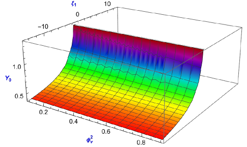
(a) (Color Online) $\xi_{2}=1$

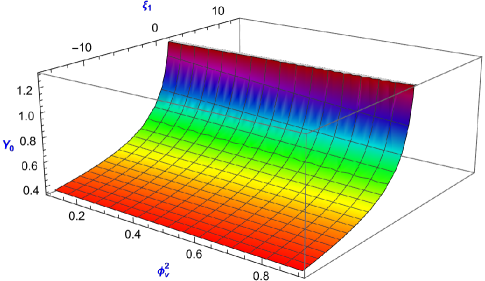
(b) (Color Online) $\xi_{2}=-1$

Figure 1: Variation of $Y_{0}$ with $\phi_{v}^{2}$ with $\xi_{2}=$ constant and $\xi_{1}$ varying

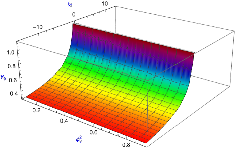
(a) (Color Online) $\xi_{1}=1$

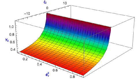
(b) (Color Online) $\xi_{1}=-1$

Figure 2: Variation of $Y_{0}$ with $\phi_{v}^{2}$ with $\xi_{1}=$ constant and $\xi_{2}$ varying

Case 2:

It has been noted that, in the limiting case, i.e., at $v\rightarrow 0$ and $r\rightarrow 0$ the value of $Y_{0\pm}$ becomes exactly the same as in case 1. We would get similar conditions (48) at the central singularity. The condition for the real solution of $Y_{0}$ becomes the same as mentioned in (51). Clearly, this is because of the choice of the constants $\beta_{1}$ and $\beta_{2}$. As a consequence, in this case, also we get a global naked singularity rather than a black hole.

Case 3:

Following the similar approach of Case 1, we compute the value of $Y(=v/r)$ at $r\rightarrow 0,v\rightarrow 0$. In this case, we get

$$\frac{2}{Y_{0}}=\lim\limits_{\begin{subarray}{c}v\to 0\\ r\to 0\end{subarray}}\Bigg{(}1-\frac{2g_{1}\Big{[}-1+2\beta_{2}(1+\sqrt{1-\phi_{v}^{2}})\Big{]}+g_{2}\Big{[}-1+2\beta_{2}(1-2n+\sqrt{1-\phi_{v}^{2}})\Big{]}}{2rg_{2}\beta_{2}n(\omega-1)\Big{[}1+\beta_{2}\Big{(}n-2(1+\sqrt{1-\phi_{v}^{2}})\Big{)}\Big{]}}\Bigg{)}.$$ (52)

The limit of the expression $\frac{2}{Y_{0}}$ diverges as $r$ approaches zero. To obtain an accurate solution for the aforementioned equation, it is necessary for the mass function to explicitly depend on both $v$ and $r$. However, in this particular scenario, this condition is not satisfied. Thus far, we have not attained any instances of a collapsing situation. However, variation of a mass parameter may be seen. Based on the variation of the mass parameter with $\phi_{v}^{2}$ and time ($v$), we may conclude that it is possible to encounter either a bouncing or accelerating scenario, as stated below.

Case 4:

Similar to case 3 here we can not study the gravitational collapse as the mass parameter (45) does not depend on $r$. But the variation of a mass parameter can be observed here too.

Now, using graphical analysis we shall discuss about the variations in the mass parameters Eqs. (42) and (45) for Cases 3 and 4. Basically, Cases 3 and 4 present fascinating scenarios which can be investigated as follows. There is a clear dependence of $\phi_{v}^{2}$ on the mass parameter $\mathcal{M}(v,r)$ in (42) and (45). When the mass parameter is plotted against $\phi_{v}^{2}$ for various values of $\omega$, the resulting graphs are denoted as Figs. 3(a) and 4(a) for instances Cases 3 and 4 respectively. We can observe that for every EOS parameter ($\omega$), the mass function reduces as $\phi_{v}^{2}$ increases, and at a particular value of $\phi_{v}^{2}\leavevmode\nobreak\ (=0.75)$, the mass function coincides with zero in two cases and varies again. It is important to note that the values of the kinetic energy of the K-essence scalar field ($\phi_{v}^{2}$) are $0<\phi_{v}^{2}<1$. The above feature can be explained as follows:

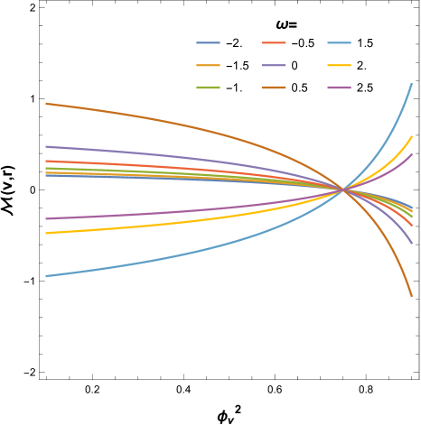
(a) (Color Online) $\mathcal{M}(v,r)$ vs $\phi_{v}^{2}$

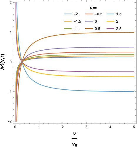
(b) (Color Online) $\mathcal{M}(v,r)$ vs $v/v_{0}$

Figure 3: Variation of mass parameter (Case 3: $\mathcal{M}(v,r)$) for different EOS parameter ($\omega$)

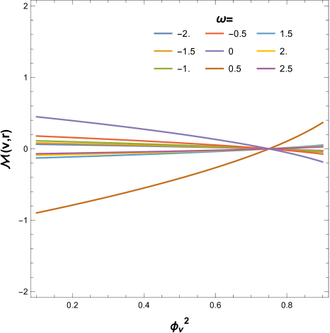
(a) (Color Online) $\mathcal{M}(v,r)$ vs $\phi_{v}^{2}$

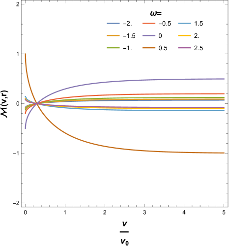
(b) (Color Online) $\mathcal{M}(v,r)$ vs $v/v_{0}$

Figure 4: Variation of mass parameter (Case 4: $\mathcal{M}(v,r)$) for different EoS parameter ($\omega$)

The K-essence idea is also used in the study of the impact of dark energy throughout the cosmos [92, 88, 146]. Furthermore, it has been shown by several observations, such as those conducted by WMAP, Planck collaborations, and IA Supernovae, etc. [24, 25, 26, 27, 28, 29], that the estimated present value of dark energy density is around $0.74$. The kinetic energy of the K-essence scalar field ($\phi_{v}^{2}$) can be employed as a representation of dark energy density in the unit of critical density [104, 105, 106, 107, 108].

So, at this point ($\phi_{v}^{2}=0.75$), the mass has been completely transformed into energy, which has caused spacetime to change into Minkowski spacetime. As a result, it is possible to argue that the universe is dominated by dark energy and that spacetime is of the Minkowski type at the point $0.75$. This phenomenon occurs exclusively when observing the cosmos from an asymptotically flat perspective. It is evident that we are now studying the emergent Vaidya spacetime as our fundamental metric, which possesses a dynamical horizon [137, 138, 139, 140], detail explained by Manna et al. [109, 110, 113]. This dynamical horizon comes through the mass function $\mathcal{M}(v,r)$ affected by the kinetic energy of the K-essence scalar field ($\phi_{v}^{2}$). The existence of dark energy implies that the expansion of the universe is accelerating, as opposed to undergoing a collapse.

Once again, there is a constraint on the value of $\phi_{v}^{2}$ where $0<\phi_{v}^{2}<1$. The variable $v$ may be represented as $\phi_{v}^{2}=e^{-v/v_{0}}\theta(v)$, as stated in the Ref. [109]. When the mass parameter is plotted against the ratio of time ($v$) to the reference time ($v_{0}$), we find Figs. 3(b) and 4(b) for Cases 3 and 4, respectively. The constant $v_{0}$ is chosen to parameterize the unit of $v$. Additionally, it is stated that Figs. 4(a) and 4(b) illustrate the variations in $\mathcal{M}(v,r)$ as a function of $\phi_{v}^{2}$ and $v/v_{0}$ respectively, assuming that $g_{1},\leavevmode\nobreak\ g_{2},\leavevmode\nobreak\ n$ are set to a value of unity for the sake of simplicity. The variation of the mass parameters with respect to time ($v$) in units of $v_{0}$ may be observed from Figs. 3(a) and 4(b). Based on the analysis of Figs. 3(b) and 4(b), it is observed that the mass parameter undergoes a growth, either positive or negative, depending on the values of the EoS parameter $\omega$, subsequent to the reaching the value $v/v_{0}=0.287682$.

Based on the aforementioned graphs, specifically Figs. 3(a), 4(a), 3(b) and 4(b), we generate two tables, denoted as Tables 1 and 2. Table 1 presents an overview of the variations in the mass parameters $\mathcal{M}(v,r)$ under different values of $\omega$ for Cases 3 and 4, specifically at $\phi_{v}^{2}=0.5$ and $\phi_{v}^{2}=0.9$. Table 2 presents the mass parameters $\mathcal{M}(v,r)$ for various values of $\omega$ in Cases 3 and 4, specifically when $\frac{v}{v_{0}}=2$.

$\omega$	Epoch	$\mathcal{M}(v,r)$
		$\phi_{v}^{2}=0.5$		$\phi_{v}^{2}=0.9$
		Case 3	Case 4	Case 3	Case 4
-2	Dark Energy era	0.0976	0.0296	-0.1937	-0.0262
-1.5	Dark Energy era	0.1171	0.0376	-0.2324	-0.0334
-1.0	Dark Energy era	0.1464	0.0518	-0.2905	-0.0459
-0.5	Dark Energy era	0.1953	0.0828	-0.3874	-0.0735
0	Dust era	0.2929	0.2071	-0.5811	-0.1838
0.5	Early Universe	0.5858	-0.4142	-1.16223	0.3675
1.0	Stiff Fluid	Diverging	-0.1035	Diverging	0.0919
1.5		-0.5858	-0.0592	1.1623	0.0525

Table 1: Table of $\mathcal{M}(v,r)$ for different $\omega$ for Cases 3 and 4 at $\phi_{v}^{2}=0.5$ and $\phi_{v}^{2}=0.9$.

$\omega$	Epoch	$\mathcal{M}(v,r)$
		$\frac{v}{v_{0}}=2$
		Case 3	Case 4
-2	Dark Energy era	0.1541	0.0614
-1.5	Dark Energy era	0.1849	0.0781
-1.0	Dark Energy era	0.2311	0.1075
-0.5	Dark Energy era	0.3082	0.1719
0	Dust era	0.4622	0.4299
0.5	Early Universe	0.9246	-0.8597
1.0	Stiff Fluid	Diverging	-0.2149
1.5		-0.9246	-0.1228

Table 2: Table of $\mathcal{M}(v,r)$ for different $\omega$ for Cases 3 and 4 at $\frac{v}{v_{0}}=2$.

According to the data shown in Table 1, it is evident that all the mass parameters exhibit positive values until the dust period, specifically at $\phi_{v}^{2}=0.5$. After that for Case 4, it is seen all values of the mass parameter are negative and for Case 3 at $\omega=0.5$, the mass parameter is positive, at $\omega=1.0$, it is diverging, and at $\omega=1.5$, it is again negative. On the other hand, when $\phi_{v}^{2}=0.9$, the majority of the mass parameter values exhibit negativity in both scenarios, but a subset of values demonstrate positivity. In both scenarios, namely before and subsequent to the current value of the dark energy density ($\phi_{v}^{2}\leavevmode\nobreak\ (=0.74)$), some mass parameters exhibit negativity. The occurrence of unforeseen properties in our scenarios can be ascribed to the presence of negative masses, which may indicate the probable existence of a gravitational dipole [143, 144] within our universe, with signs of future expansion. In this discourse, we explore the concepts of positive and negative mass in contemporary contexts.

The concept of negative mass has been explored in several scholarly publications [141, 144, 142, 143, 145] within various contexts. It is pointed out that Bondi and Bonnor [143, 145] in their articles elaborately discussed the existence of negative mass along with the positive mass. In his work, Miller [144] provides a description of negative-mass lagging cores within the context of the big bang. The author stated that for very high values of the geometrically specified coordinate $r$, the mass is positively valued, whereas, at considerably small values of $r$, the mass is negatively valued. The area of spacetime characterized by negative mass has local features that resemble those observed in the negative-mass Vaidya solution. The author may endeavor to establish a nonsingular past for the given hypersurface. Consider a possible scenario in which we have a celestial object composed exclusively of particles that undergo decay, resulting in the emission of photons that subsequently dissipate. The description of the spacetime outside the contracting star is effectively explained by a Vaidya solution, whereby the relationship between the mass and the outgoing null coordinate $v$ is established based on the rate of particle disintegration.

In his article, the occurrence of the big bang is characterized by a combination of spacelike and timelike properties, resulting in spacetimes that do not adhere to the stringent version of the cosmic censorship hypothesis. In the context of general-relativistic cosmology, it is explicitly acknowledged that the big bang might potentially possess both spacelike and timelike characteristics. This implies that a portion of the big bang event may have been influenced by factors originating inside spacetime itself. In these basic spherically symmetric models, the timelike section of the big bang is characterized by a negative mass and serves as an inexhaustible reservoir of energy, manifesting as gravitational and electromagnetic radiation. If compact and numerous sources of energy were to exist, they may potentially contribute to the understanding of several cosmic events characterized by high levels of energy. On the other hand, in his article [144], in the negative-mass Schwarzschild solution, it can be observed that the singularity located at $r=0$ is intersected by both the future and past light cones at any given position. This implies that the singularity possesses a timelike nature. Therefore, it may be concluded that spacetime does not adhere to the stringent version of the cosmic censorship theory, which posits the absence of timelike singularities, whether they originated from primordial conditions or emerged from initially non-singular circumstances. Bondi [143] has identified a notable phenomenon known as the “gravitational dipole,” which is defined by the presence of both a positive mass and a negative mass. Positive mass exhibits attractive behavior towards negative mass, whereas negative mass demonstrates repulsive behavior towards the positive mass. Consequently, both masses experience acceleration in a corresponding direction, resulting in the negative mass pursuing the positive mass, leading to the attainment of exceptionally high velocities by the dipole. Also, it should be noted that in our generalized emergent Vaidya spacetime (19), the removal of the $\phi_{v}^{2}$ term and the substitution $\mathcal{M}(v,r)\equiv m(v)$ as well as not considering $f(\bar{R},\bar{T})$ gravity, which corresponds to the conventional Vaidya spacetime, leads us back to the investigation conducted by Miller in his published work [144], which established the existence of both the positive and negative masses.

Table 2 also presents the positive and negative aspects of the mass parameter, contingent upon the values of the EOS parameter. This observation further suggests the presence of dark energy and gravitational dipole across the many epochs of the cosmos, as shown by the presence of both negative and positive mass parameters, which are contingent upon the specific value of the EOS parameter. It should be also noted that a negative value of the EOS parameter indicates a world that is predominantly dominated by dark energy. Typically, the EOS parameter value for a dark energy-dominated universe is considered as -1 and a larger negative value signifies a greater dominance of dark energy in the universe. The EOS parameter zero is often known as the dust or matter-dominated epoch. A value of $0.5$ indicates scenarios pertaining to the early universe, whereas a value of $1.0$ corresponds to the stiff fluid era. The presence of a negative mass parameter, coupled with a positive EOS parameter, suggests the possibility of the occurrence of negative mass during the early stages of the cosmos. On the other hand, the appearance of a gravitational dipole and dark energy characterized by negative EoS parameters demonstrate the phenomenon of late-time acceleration in the cosmos. According to Bondi [143], it can be asserted that in our particular model, the gravitational dipole is also present. This implies that in our model, both negative and positive masses simultaneously exist, given the specific choices of $f(\bar{R},\bar{T})$ as outlined in Eqs. (40) and (43), subject to certain fixed constants. So, we can say that under the concept of a gravitational dipole, there exists a dark energy-dominated universe, implying that the world is accelerating.

V Conclusion

In this section, we provide an overview of our research findings, which may be summarised as follows: The emergent $f(\bar{R},\bar{T})$ gravity in the K-essence geometry was initially taken into consideration. The Lagrangian employed in this study is a non-canonical Lagrangian of the DBI type, as shown by Eq. (8). Additionally, the modified field equation associated with this theory, represented by Eq. (17), corresponds to the emergent energy-momentum tensor ($\bar{T}_{\mu\nu}$) as indicated in Eq. (14). This part has been summarised in section II. On the other hand, we have also taken into account the emergent Vaidya spacetime as our primary metric (19), while specifying the mass function in (20) and the energy-momentum tensor in (26). In accordance with the reference [110] , several matter-dependent parameters, namely $\bar{\gamma}$, $\bar{\rho}$, $\bar{p}$, have been introduced. These parameters correspond to the energy density associated with the emergent Vaidya null radiation, as well as the energy density and pressure of the emergent perfect fluid, respectively. Note that the mass parameter in this context has been considered as a function of $r$ and $v$, where $v$ represents the null coordinate associated with the Eddington advanced time. The value of $r$ decreases towards the future along a ray that is associated with a constant value of $v$. The temporal variation of the emergent mass function ($\mathcal{M}(v,r)$) arises from the generalized Vaidya mass ($m(v,r)$) in the background, as well as the kinetic energy associated with the K-essence scalar field ($\phi_{v}^{2}$). The functional form of $f(\bar{R},\bar{T})$ is seen as an additive composition of two functions, namely $f_{1}(\bar{R})$ which only relies on the Ricci scalar ($\bar{R}$), and $f_{2}(\bar{T})$ which solely relies on the trace of the energy-momentum tensor ($\bar{T}$). By referencing the field equations in (28), (29), and (30), we go to the subsequent stage of our study. In our analysis, we focus on the $(22)$ or $(33)$ component of the field equation in order to create a comprehensive model.

In the subsequent section, section III, we analyze four models of the $f(\bar{R},\bar{T})$ theory and determine the solution for the generalized mass parameter, denoted as $\mathcal{M}(v,r)$, for each of the above cases: Case 1 (Eq. 34), Case 2 (Eq. 39), Case 3 (Eq. 42) and Case 4 (Eq. 45). The solutions for Cases 1 and 2 give identical findings given the specified conditions on $\beta_{1}$, $\beta_{2}$, $g_{1}$, and $g_{2}$. Whereas the solutions in Cases 3 and 4 exhibit similarities under certain particular circumstances on the parameters. In our proposed model, the mass functions exhibit an additional K-essence-related component, denoted as $(\phi_{v}^{2})$, which distinguishes it from the general case. This unique characteristic encourages us to investigate the remarkable behavior of the mass function, as discussed in Section IV.

In Section IV we study the underlying physics of the mass parameters obtained in the previous section. The mass functions in Cases 1 and 2 have an explicit dependency on $r$, allowing us to study the gravitational collapse and the fate of singularity. The limiting conditions on the tangent of the radial null geodesic (47) tell us that the singularity formed in our case is naked for any value of $\phi_{v}^{2}$. Figures (1(a)), (1(b)), (2(a)) and (2(b)) supports the statement. In this procedure, we check all the possible values of the constants $\xi_{1}$ and $\xi_{2}$. On the way, we have established the condition (51) for which the solution of Eq. (49) is real.

The study of the mass function pertaining to Cases 3 and 4 yields surprising results. Initially, it should be noted that the solutions of the mass function do not explicit dependence on the variables $r$ or $v$. Consequently, these solutions are unable to offer any information about the singularity. However, their dependence relies on the K-essence term $\phi_{v}^{2}$, which exhibits a temporal dependency on the variable $v$. In the aforementioned scenarios, the mass parameters exhibit a non-constant nature, since they are implicitly dependent on time due to the presence of the kinetic energy term ($\phi_{v}^{2}$) associated with the K-essence scalar field. When we plot the mass function with $\phi_{v}^{2}$ for different $\omega$ we get that in each case the mass function reaches to zero at a particular value of $\phi_{v}^{2}$, which is $0.75$ (3(a) $\&$ 4(a)). Now according to the observation, we know that the present value of dark energy is about $0.74$. That means the K-essence term $\phi_{v}^{2}$ can be considered as the dark energy component of the universe [104, 105, 106, 107, 108]. The mass function vanishes at the point $0.75$. This is a clear indication that the mass has been converted into energy at this point indicating that the spacetime we are now is Minkowski. We should remember the fact that we started with a generalized Vaidya spacetime in the context of K-essence geometry. Surprisingly it is seen that this phenomenon occurs within the context of flat spacetime in the current era of our universe, specifically for a certain value of $\phi_{v}^{2}$. Again the condition that makes the spacetime (19) physical is that $\phi_{v}^{2}$ can have a value between $0$ and $1$. This enables us to consider it as an exponential function of $v/v_{0}$ ($\phi_{v}^{2}=e^{-v/v_{0}}\theta(v)$), which provides us with the scope to study the variation of mass parameter with respect to the normalized time coordinate $v/v_{0}$ (Figs. 3(b) and 4(b)). The zero point of mass function arises at around $0.287682$ in the $v/v_{0}$ axis intending the similar behavior of the mass function as achieved with $\phi_{v}^{2}$. In these figures, we see the mass function sometimes becomes positive and sometimes negative depending upon the value of $\omega$ we choose. Two tables (1) and (2) have been arranged to study the behavior of the mass function in these two cases namely, Cases 3 and 4. In conclusion, it is important to reiterate that the presence of a positive and negative mass function in this study may potentially signify the existence of a gravitational dipole across various stages of the universe. Each curve on these graphs encompasses both positive and negative values of the mass function, either before or succeeding the zero value. The potential existence of this gravitational dipole might perhaps account for the phenomenon of early inflation and the subsequent accelerated expansion of the cosmos.

It is noteworthy to emphasize that the K-essence theory possesses the capability to be utilized in a complete way, enabling the concurrent investigation of both dark energies [92, 88, 104, 105, 106, 146] and a purely gravitational perspective [109, 110, 112, 113]. The findings supporting the existence of dark energy, a Minkowski universe for a fixed point, and the gravitational dipole in our study agree well with the postulated theories. Additionally, our research provides evidence for the existence of a global naked singularity by examining gravitational collapse just from a gravitational perspective, without considering the dark energy density represented by $\phi_{v}^{2}$. Therefore, it can be concluded that the K-essence theory possesses the potential to serve as both a dark energy framework and a simply gravitational theory simultaneously, facilitating the examination of diverse phenomena within the realm of cosmology.

References

- [1] P. S. Joshi, Pramana J. Phys. 55, 529 (2000).
- [2] P. S. Joshi, Global Aspects in Gravitation and Cosmology, Clarendon, Oxford (1993).
- [3] J. R. Oppenheimer et al., Phys. Rev. 56, 455 (1939).
- [4] D. Malafarina, Universe 3, 48 (2017).
- [5] R. Penrose, Riv. Nuovo Cim. 1, 252 (1969).
- [6] R. Penrose, Gen. Rel. Grav. 34, 1141 (2002).
- [7] D. M. Eardley et al., Phys. Rev. D 19, 2239 (1979).
- [8] D. Christodoulou, Commun. Math. Phys. 93, 171 (1984).
- [9] R. P. A. C. Newman, Class. Quantum Grav. 3, 527 (1986).
- [10] I. H. Dwivedi et al., Class. Quantum Grav. 9, L39 (1992).
- [11] P. S. Joshi, et al., Phys. Rev. D 47, 5357 (1993).
- [12] P. S. Joshi et al., Commun. Math. Phys. 146, 333 (1992).
- [13] P. S. Joshi et al., Phys. Rev. D 51, 6778 (1995).
- [14] B. Waugh et al., Phys. Rev. D 34, 2978 (1986).
- [15] A. Ori et al., Phys. Rev. D 42, 1068 (1990).
- [16] K. Lake, Phys. Rev. Lett. 68, 3129 (1992).
- [17] P. Szekeres et al., Phys. Rev. D 47, 4362 (1993).
- [18] P. C. Vaidya, Proc. Indian Acad. Sci. Sect. A 33, 264 (1951).
- [19] P. Rudra et al., Nucl. Phys. B 909, 725 (2016).
- [20] Y. Heydarzade et al., Phys. Lett. B 774, 46 (2017).
- [21] P. Rudra et al., Eur. Phys. J. C 78, 828 (2018).
- [22] P. Rudra, Int. J. Mod. Phys. D 31, 13, 2250095 (2022).
- [23] Y. Heydarzade, et al., J. Cosmol. Astropart. Phys. 06, 038 (2018).
- [24] A. G. Riess et al., Astron. J. 116, 1009 (1998).
- [25] S. Perlmutter et al., Astroph. J. 517, 565 (1999).
- [26] E. Komatsu et al., Astroph. J. Suppl. 192, 18 (2011).
- [27] P. A. R. Ade et al. (Planck Collaboration), A A 594, A14 (2016).
- [28] N. Aghanim et al. (Planck Collaboration), A A 641, A6 (2020).
- [29] N. Aghanim et al. (Planck Collaboration), N. Aghanim et al., A A 641, A1 (2020).
- [30] S. M. Carroll et al., Phys. Rev. D 70, 043528 (2004).
- [31] V. K. Oikonomou, Phys. Rev. D 103, 124028 (2021).
- [32] V. K. Oikonomou et al., Int. J. of Mod. Phys. D 31, 2250075 (2022).
- [33] T. P. Sotiriou et al., Rev. Mod. Phys. 82, 451 (2010).
- [34] A. De Felice et al., Living Rev. Rel. 13, 3 (2010).
- [35] S. Nojiri et al., Int. J. Geom. Meth. Mod. Phys. 4, 115 (2007).
- [36] S. Nojiri et al., J. Phys. Conf. Ser. 66, 012005 (2007).
- [37] S. Nojiri et al., Phys. Rev. D 74, 086005 (2006).
- [38] S. Capozziello et al., Phys. Lett. B 632, 597 (2006).
- [39] S. Nojiri et al., Phys. Lett. B 657, 238 (2007).
- [40] E. Elizalde et al., Phys. Rev. D 77, 106005 (2008).
- [41] G. Cognola et al., Class. Quantum Grav. 27, 095007 (2010).
- [42] R. Myrzakulov et al., Gen. Relativ. Gravit. 43, 1671 (2011).
- [43] R. Durrer et al., arXiv:0811.4132.
- [44] E. J. Copeland et al., Int. J. Mod. Phys. D. 15, 1753 (2006).
- [45] T. Harko et al., Eur. Phys. J. C 70, 373 (2010).
- [46] T. Harko et al.,Phys. Rev. D 84, 024020 (2011).
- [47] P. K. Sahoo et al., Eur. Phys. J. Plus 131, 333 (2016).
- [48] G. Alvarenga et al., Phys. Rev. D 87, 103526 (2013).
- [49] M. Sharif et al., Phys. Dark Univ. 15, 105 (2017).
- [50] M. Sharif et al., J. Cosmol. Astropart. Phys. 03, 028 (2012).
- [51] G. P. Singh et al., Astrophys. Space Sci. 360, 34 (2015).
- [52] G. P. Singh et al., Adv. High Energy Phys. 2015, 816826 (2015).
- [53] E. Baffou et al., Eur. Phys. J. C 79, 112 (2019).
- [54] S. Aygun et al., Grav. and Cosmol. 24, 302 (2018).
- [55] S. Sahu et al., Chin. J. Phys. 55, 862 (2017).
- [56] J. Satish et al., Chin. J. Phys. 54, 830 (2016).
- [57] B. Mirza et al., Int. J. Geom. Meth. in Mod. Phys. 13, 1650108 (2016).
- [58] M. J. S. Houndjo, Int. J. Mod. Phys. D 21, 1250003 (2012).
- [59] M. J. S. Houndjo et al., Int. J. Mod. Phys. D 21, 1250024 (2012).
- [60] M. Jamil et al., Euro. Phys. J. C 72, 1999 (2012).
- [61] A. de la C. Dombriz et al., Class. Quantum Grav. 29, 245014 (2012).
- [62] S. Nojiri et al., Phys. Lett. B 681, 74 (2009).
- [63] M. J. S. Houndjo et al., Can. J. Phys. 91,(7), 548 (2013).
- [64] P. H. R. S. Moraes et al., Eur. Phys. J. C 79, 677 (2019).
- [65] M. Zubair et al., Astroph. Space Sci. 361, 238 (2016).
- [66] G. P. Singh et al., Int. J. Geom. Meth. in Mod. Phys. 13, 1038 (2016).
- [67] M. Zubair et al., Eur. Phys. J. C 77, 680 (2017).
- [68] M. Zubair et al, Astrophys. Space Sci. 349, 457 (2014).
- [69] M. Zubair et al, Phys. of the Dark Univ. 28, 100531 (2020).
- [70] J.K. Singh et al., Ann. Phys. 443, 168958 (2022).
- [71] T. Clifton et al., Phys. Rept. 513, 1 (2012).
- [72] E. Fradkin et al., Phys. Lett. B 189, 89 (1987).
- [73] M.A. Vasiliev, Phys. Lett. B 243, 378 (1990).
- [74] J. Khoury et al., Phys. Rev. D 69 044026 (2004).
- [75] J. Khoury et al., Phys. Rev. Lett. 93, 171104 (2004).
- [76] A.I. Vainshtein, Phys. Lett. B 39, 393 (1972).
- [77] W. Horndeski, Int. J. Theor. Phys. 10, 363 (1974).
- [78] C. Deffayet et al., Phys. Rev. D 84, 064039 (2011).
- [79] Tiago B. Gonçalves et al. Phys. Rev. D 105, 064019 (2022).
- [80] J. L. Rosa, Phys. Rev. D 103, 104069 (2021).
- [81] N. C. Rana and P. S. Joag, Classical Mechanics, McGraw Hill Education (India) Private Limited (1991).
- [82] A. K. Raychaudhuri, Classical Mechanics: A course of Lectures, Oxford University Press (1983).
- [83] H. Goldstein, Classical Mechanics, 2nd Edition, Narosa Publishing House (2000).
- [84] P. Jiroušek et. al., J. High Energy Phys. 07, 154 (2023)
- [85] M.Visser et al., Gen. Rel. Grav. 34, 1719 (2002).
- [86] E. Babichev et al., J. High Energy Phys. 02, 101 (2008).
- [87] E. Babichev et al., J. High Energy Phys. 0802, 101 (2008).
- [88] A. Vikman, K-essence: Cosmology, causality and Emergent Geometry, Dissertation an der Fakultatfur Physik,Arnold Sommerfeld Center for Theoretical Physics, der Ludwig-Maximilians-Universitat Munchen, Munchen (2007).
- [89] E. Babichev et al, Looking beyond the Horizon, WSPC Proceedings (2008).
- [90] L. P. Chimento et al., Phys. Rev. D 69, 123517 (2004).
- [91] C. Armendariz-Picon et al., Phys. Rev. D 63, 103510 (2001).
- [92] R. J. Scherrer, Phys. Rev. Lett. 93, 011301 (2004).
- [93] L. P. Chimento, Phys. Rev. D 69, 123517 (2004).
- [94] C. Armendariz-Picon et al., Phys. Rev. Lett. 85, 4438 (2000).
- [95] C. Armendariz-Picon et al., Phys. Lett. B 458, 209 (1999).
- [96] S. X. Tian and Z.-H. Zhu, Phys. Rev. D, 103, 043518 (2021).
- [97] R. Myrzakulov and L. Sebastiani, Symmetry 8, 57 (2016).
- [98] A. A. Sen and N. C. Devi, Gen. Relativ. Gravit. 42, 821 (2010).
- [99] A. Chatterjee et al., Phys. Rev. D 104, 103505 (2021)
- [100] Velten et el., The Eur. Phys. J. C. 74, 3160 (2014).
- [101] J. K. Erickson et al., Phys. Rev. Lett. 88, 121301 (2002).
- [102] S. Dedeo et al., Phys. Rev. D 67, 103509 (2003).
- [103] R. Bean et al., Phys. Rev. D 69, 083503 (2004).
- [104] D. Gangopadhyay and G. Manna, Euro. Phys. Lett. 100, 49001 (2012).
- [105] G. Manna and D. Gangopadhyay, Eur. Phys. J. C 74, 2811 (2014).
- [106] G. Manna and B. Majumder, Eur. Phys. J. C 79, 553 (2019).
- [107] G. Manna et al., Eur. Phys. J. Plus 135, 107 (2020).
- [108] G. Manna et al., Chinese Phys. C 47, 025101 (2023).
- [109] G. Manna et al., Phys. Rev. D 101, 124034 (2020).
- [110] G. Manna, Eur. Phys. J. C 80, 813 (2020).
- [111] S. Ray et al., Chinese Phys. C 46, 12, 125103 (2022).
- [112] S. Das et al., Fortschr. Phys. 71, 2200193 (2023).
- [113] B. Majumder et al., Fortschr. Phys. 2300133 (2023).
- [114] Shinji Mukohyama et al., Phys. Rev. D 94, 023514 (2016).
- [115] M. Born et al. Proc. Roy. Soc. Lond. A 144, 425 (1934).
- [116] W. Heisenberg, Zeit. Phys. 113, 61 (1939).
- [117] P. A. M. Dirac, Proc. Roy. Soc. Lond. A 268, 57 (1962).
- [118] A. D. Linde, Phys. Lett. B 108, 389 (1982).
- [119] A. Albrecht et al., Phys. Rev. Lett. 48, 1220 (1982).
- [120] G. Dvali et al., Phys. Lett. B 450, 72 (1999).
- [121] S. Kachru et al., J. Cosmol. Astropart. Phys. 0310, 013 (2003).
- [122] M. Alishahiha et al., Phys. Rev. D 70, 123505 (2004).
- [123] E. Silverstein et al., Phys. Rev. D 70, 103505 (2004).
- [124] X. Chen, Phys. Rev. D 71, 063506 (2005).
- [125] S. Weinberg, Phys. Rev. D 77, 123541 (2008).
- [126] X. Chen et al., J. Cosmol. Astropart. Phys. 0701, 002 (2007).
- [127] A. Panda et al., arxiv: 2206.14808 (2023)
- [128] J. T. Nielsen, A. Guffanti, S. Sarkar, Sci. Rep. 2016, 6, 3559.
- [129] P. R. Ade, et al. (Planck Collaboration), Astron. Astrophys. 2016, 594, 20.
- [130] V. Husain, Phys. Rev. D 53, 4 (1996).
- [131] D. Mkenyeleye et al., Phys. Rev. D 90, 064034 (2014).
- [132] A. Wang et al., Gen. Relativ. Grav. 31, 1 (1999).
- [133] S. W . Hawking and G. F. R. Ellis, The Large Scale Structure of Spacetime, Cambridge University Press, Cambridge (1973)
- [134] J. de Boer et al., SciPost Phys. 5, 003 (2018)
- [135] M. S. Khan, S. Khan, Gen. Rel. Grav. 51, 148 (2019).
- [136] G. Abbas and R. Ahmed, Mod. Phys. Lett. A 34, 20, 1950153 (2019)
- [137] S. A. Hayward, Phys. Rev. D 49, 6467 (1994).
- [138] A. Ashtekar and B. Krishnan, Phys. Rev. D 68, 104030 (2003).
- [139] A. Ashtekar and B. Krishnan, Phys. Rev. Lett. 89, 261101 (2002).
- [140] A. Ashtekar and B. Krishnan, Living Rev. Relativity 7, 10 (2004).
- [141] S. Najera et al., A & A 651, L13 (2021).
- [142] V. Vertogradov, Universe 6, 155 (2020).
- [143] H. Bondi, Rev. Mod. Phys. 29, 423 (1957).
- [144] B. D. Miller, Astrophys. J. 208, 275-285 (1976).
- [145] W. B. Bonnor, Gen. Relat. Gravit. 21, 1143 (1989).
- [146] J. Yoo and Y. Watanabe, Int. J. Mod. Phys. D 21, 12, 1230002 (2012).