The quantum connection, Fourier-Laplace
transform, and families of $A_{\infty}$-categories

Abstract.

Consider monotone symplectic manifolds containing a smooth anticanonical divisor. Contingent on conjectures which relate quantum cohomology to the symplectic cohomology of the divisor complement (à la Borman-Sheridan-Varolgunes), we show that the quantum connection has unramified exponential type. The argument involves wrapped Fukaya categories, the regularity theorem of Petrov-Vaintrob-Vologodsky in noncommutative geometry, and a new categorical interpretation of the Fourier-Laplace transform of $D$-modules.

1. Introduction

1.1. The quantum connection

Our discussion will be limited to the smallest, which means single-parameter, version of the quantum connection. (Readers interested in a wider picture may want to look at e.g. [28, 29, 47].) Let $M$ be a closed symplectic manifold which is monotone,

(1.1.1) $$[\omega_{M}]=c_{1}(M)\in H^{2}(M;{\mathbb{R}}).$$

Let $q$ be a formal variable of degree $2$. The quantum connection on $H^{*}(M;{\mathbb{C}})[q^{\pm 1}]$ is the following ${\mathbb{Z}}/2$-graded endomorphism, which differentiates with respect to the variable $q$:

(1.1.2) $$\nabla_{\partial_{q}}x=\partial_{q}x+q^{-1}([\omega_{M}]\ast_{q}x),$$

where $\ast_{q}$ is the small quantum product,

(1.1.3) $$x\ast_{q}y=x\ast^{(0)}y+q\,x\ast^{(1)}y+q^{2}\,x\ast^{(2)}y+\cdots$$

The term $\ast^{(k)}$, which counts rational curves with first Chern number $k$, has degree $-2k$; for $k=0$, it is the classical (cup) product. Therefore, the quantum connection has a simple pole at $q=0$, with nilpotent monodromy $x\mapsto[\omega_{M}]x$. This is a non-resonant case, so the monodromy is conjugate to $x\mapsto\exp(-2\pi i[\omega_{M}]x)$. One can simplify the $q$-dependence in (1.1.2) as follows. Take a grading operator

(1.1.4) $$\mathrm{Gr}:H^{*}(M;{\mathbb{C}})\longrightarrow H^{*}(M;{\mathbb{C}}),$$

which multiplies the degree $d$ cohomology by some even integer $\delta_{d}$ such that $\delta_{d+2}=\delta_{d}+2$. (If there is no odd degree cohomology, one can take $\delta_{d}=d$; or in general, $\delta_{d}=2\lfloor d/2\rfloor$.) Then (1.1.2) is gauge equivalent to

(1.1.5) $$\nabla_{\partial_{q}}^{\mathrm{Gr}}x\stackrel{{\scriptstyle\mathrm{def}}}{{=}}(q^{\mathrm{Gr}/2\,}\nabla_{\partial_{q}}\,q^{-\mathrm{Gr}/2})(x)=\partial_{q}x-q^{-1}\frac{\mathrm{Gr}(x)}{2}+[\omega_{M}]\ast x,$$

where $\ast$ without subscript means that we set $q=1$ in (1.1.3). (In the literature, e.g. [28], odd values of $\delta_{d}$ are often used, leading to a gauge transformation involving $q^{1/2}$.) We are interested in the behaviour near $q=\infty$, and therefore change variables to $Q=1/q$. The quantum connection (multiplied by $-q^{2}$, to account for the difference between the vector fields $\partial_{q}$ and $\partial_{Q}$) is correspondingly written as

(1.1.6) $$\nabla_{\partial_{Q}}x=\partial_{Q}x-Q^{-1}([\omega_{M}]\ast_{Q^{-1}}x),$$

(1.1.7) $$\nabla_{\partial_{Q}}^{\mathrm{Gr}}x=\partial_{Q}x-Q^{-2}([\omega_{M}]\ast x)+Q^{-1}\frac{\mathrm{Gr}(x)}{2}.$$

In (1.1.7), the pole order has been reduced to $2$, which in general is the best one can do by gauge transformations: the $Q=0$ singular point is usually not regular. Such quadratic singularities have a rich structure, of which we consider only the part remembered in formal power series expansion in $Q$ (which means ignoring the Stokes phenomenon).

Conjecture 1.1.1.

(i) $\nabla_{\partial_{q}}$ has a singularity of unramified exponential type at $q=\infty$.

(ii) The regularized formal monodromies at $q=\infty$ are quasi-unipotent (their eigenvalues are roots of unity).

The terminology (unramified exponential type, regularized monodromy) will be explained in Section 2.1. The statement (i) occurs in several places in the literature, motivated by mirror symmetry: e.g. as a small piece of [49, Conjecture 3.4], or in [28, Section 2.5]. (In both of those references, it is qualified by warnings: [49, Remark 3.5(ii)] suggests restricting it to the algebro-geometric case of Fano varieties, while [28] talks of “a wide class of Fanos”.) Part (ii) is less familiar, but closely related to (i). Known partial results include:

• If the endomorphism $[\omega_{M}]\ast$ is semisimple, (i) holds for elementary reasons; see Lemma 2.1.7(ii). In the case where the quantum cohomology ring is semisimple (a direct sum of copies of the ring ${\mathbb{C}}$), a much stronger version of (ii) holds, by a purely Gromov-Witten theory argument due to Dubrovin; see Lemma 2.1.16.

• For manifolds where the quantum connection has been computed, one can verify the conjectures by hand. More conceptually, when quantum cohomology has a mirror description in terms of a superpotential, one can apply algebro-geometric methods to the Gauss-Manin connection of that superpotential, and then derive conclusions about the quantum connection by a Fourier-Laplace transform (this is the motivation mentioned above). We refer to Section 2.2 for further explanation of that strategy, which has seen extensive use in the literature. For instance, (i) is proved for certain complete intersections in projective space in [73, Proposition 7.4], based on results in [64]. This method extend to cases which are not covered by the previously mentioned self-contained arguments (even for Fano toric manifolds, the quantum cohomology can fail to be semisimple [59, Remark 5.1]). As for future outlook, one could hope to apply such arguments in the context of the “intrinsic mirror symmetry” of Gross-Siebert, where $M$ admits a (singular) anticanonical divisor $D$ which makes it into a maximal log Calabi-Yau pair [41, Definition 2.7].

• For any $\lambda\in{\mathbb{C}}$ we have a Fukaya category $\mathit{Fuk}_{\lambda}(M)$, which is a ${\mathbb{Z}}/2$-graded $A_{\infty}$-category over ${\mathbb{C}}$. This category is zero unless $\lambda$ is an eigenvalue of $[\omega_{M}]\ast$. The cyclic open-closed map [32] is a map from negative cyclic homology to ordinary (co)homology, more precisely a $u$-linear map

  (1.1.8) $$\bigoplus_{\lambda}\mathit{HC}_{*}(\mathit{Fuk}_{\lambda}(M))\longrightarrow H^{*+\mathrm{dim}_{{\mathbb{C}}}(M)}(M;{\mathbb{C}})[u].$$

  Let’s adjoin $u^{-1}$. Then, on the left hand side (periodic cyclic homology) we have a connection in the $u$-variable, with a quadratic pole [49, 83] which has nilpotent leading order term [5]. Adjust that connection by adding $\lambda u^{-2}$ times the identity on each summand (this reflects the fact that $\mathit{Fuk}_{\lambda}(M)$ should really be thought of as a curved $A_{\infty}$-category, with a curvature term which is $\lambda$ times the identity). On the right hand side, the corresponding connection should be a version of (1.1.7), with our definition of grading operator operator replaced by $\delta_{d}=d-\mathrm{dim}_{{\mathbb{C}}}(M)$; this correspondence has been proved under simplifying technical assumptions in [46]. Suppose that we are in the situation of a generation result such as [30, Theorem 3], where (1.1.8) is an isomorphism. Then we can infer properties of our connection from ones of the Fukaya category. This approach overlaps with the previous method in situations where homological mirror symmetry has been established.

1.2. Assumptions

Our approach relies on the existence of an anticanonical divisor which is smooth (unlike the situation in the Gross-Siebert program), more precisely:

Assumption 1.2.1.

$M$ contains a smooth symplectic hypersurface $D$ (integrally) Poincaré dual to $c_{1}(M)$, such that the completed complement of $D$, which a priori is a Liouville manifold, is actually (finite type) Weinstein.

In the algebro-geometric context, if $M$ is Fano and $D$ is an anticanonical divisor, $M\setminus D$ is affine and hence automatically Weinstein.

Remark 1.2.2.

Still in algebraic geometry, it is known that every Fano manifold of complex dimension $\leq 3$ has a smooth anticanonical divisor [84]. In complex dimensions $\leq 5$, it is known that anticanonical divisors exist [50, Theorem 5.2] and [43]), and conjecturally the same is true in all dimensions [50, Conjecture 2.1]; however, there may not be any smooth ones (see [44, Example 2.12] or [74, Example 2.9]). Whether that failure of smoothness is relevant for our purposes remains unclear (there can be smoothings in the symplectic world which are precluded algebro-geometrically; for instance, deforming the Fano does not change the underlying symplectic manifold).

We now introduce two conjectures in Hamiltonian Floer theory. They are closely related to recent work of Borman-Sheridan-Varolgunes [8], in that they relate the symplectic cohomology of $M\setminus D$ to the quantum cohomology of $M$. The second conjecture is an $S^{1}$-equivariant refinement of the first (as in (1.1.8), $u\in H^{2}_{S^{1}}(\mathit{point})$ is the equivariant parameter), with an additional compatibility condition. We will not make any attempt to justify the conjectures (but in Section 7.3, we set up a toy model which provides some motivation).

Conjecture 1.2.3.

Let $H_{q}$ be the graded ${\mathbb{C}}[q]$-module obtained by deforming the symplectic cohomology of $M\setminus D$ by the Borman-Sheridan class. Then,

(1.2.1) $${\mathbb{C}}[q^{\pm 1}]\otimes_{{\mathbb{C}}[q]}H_{q}\cong H^{*}(M;{\mathbb{C}})[q^{\pm 1}].$$

Conjecture 1.2.4.

Let $H_{q,u}$ be the graded ${\mathbb{C}}[q,u]$-module obtained by deforming the $S^{1}$-equivariant symplectic cohomology of $M\setminus D$ by the Borman-Sheridan class. Then,

(1.2.2) $${\mathbb{C}}[q^{\pm 1}]\otimes_{{\mathbb{C}}[q]}H_{q,u}\cong H^{*}(M;{\mathbb{C}})[q^{\pm 1},u].$$

Moreover, this isomorphism relates the canonical connection on the left, with the following version of the quantum connection on the right:

(1.2.3) $$\nabla_{u\partial_{q}}x=u\partial_{q}x+q^{-1}([\omega_{M}]\ast_{q}x).$$

Concerning Conjecture 1.2.3, what we will actually use are two somewhat weaker and technically distinct statements, see Theorem 1.3.1 (those two versions should be equivalent to each other, and also easier to prove than the full statement); and that comes in at an earlier point in the argument than Conjecture 1.2.4, which explains the separate statements. Concerning Conjecture 1.2.4, note that if we invert $u$ and consider $\nabla_{u\partial_{q}}$ as acting on $H^{*}(M;{\mathbb{C}})[q^{\pm 1},u^{\pm 1}]$, then it turns into the standard quantum connection $\nabla_{\partial_{q}}$. More precisely, for any even $d$, one can identify the degree $d$ part of $H^{*}(M;{\mathbb{C}})[q^{\pm 1},u^{\pm 1}]$ with $H^{\mathrm{even}}(M;{\mathbb{C}})[q,q^{-1}]$, by setting $u=1$; and that identification is compatible with connections. The same holds for odd $d$ and $H^{\mathrm{odd}}(M;{\mathbb{C}})[q,q^{-1}]$.

Remark 1.2.5.

It is instructive to look at (1.2.3) without inverting $u$, since that provides a more organic explanation for the gauge transformations used in (1.1.5). Take the degree zero parameter $\bar{q}=q/u$, so that $H^{*}(M;{\mathbb{C}})[q^{\pm 1},u]\cong H^{*}(M;{\mathbb{C}})[q^{\pm 1},\bar{q}^{-1}]$. For any $d\in{\mathbb{Z}}$, setting $q=1$ yields an identification

(1.2.4) $$\text{degree $d$ part of }H^{*}(M;{\mathbb{C}})[q^{\pm 1},\bar{q}^{-1}]\cong\begin{cases}H^{\mathrm{even}}(M;{\mathbb{C}})[\bar{q}^{-1}]&\text{$d$ even,}\\ H^{\mathrm{odd}}(M;{\mathbb{C}})[\bar{q}^{-1}]&\text{$d$ odd.}\end{cases}$$

Under that, (1.2.3) turns into

(1.2.5) $$\nabla_{\partial_{\bar{q}}}x=\partial_{\bar{q}}x+\bar{q}^{-1}\textstyle\frac{d-j}{2}x+[\omega_{M}]\ast x\quad\text{for }x\in H^{j}(M;{\mathbb{C}})[\bar{q}^{-1}].$$

In this way, different $d$ correspond to different choices of the grading operator in (1.1.5). Passing to $\bar{Q}=\bar{q}^{-1}=u/q$ yields the counterpart of (1.1.7), which is

(1.2.6) $$\nabla_{\partial_{\bar{Q}}}x=\partial_{\bar{Q}}x-\bar{Q}^{-2}([\omega_{M}]\ast x)+\bar{Q}^{-1}\textstyle\frac{j-d}{2}x\quad\text{for }x\in H^{j}(M;{\mathbb{C}})[\bar{Q}].$$

1.3. Results

Here’s our main result towards Conjecture 1.1.1, as well as an addendum which concerns a sharpened version of part (ii) of that conjecture.

Theorem 1.3.1.

Let $M$ be as in Assumption 1.2.1. Suppose that Conjecture 1.2.4 holds, and so do two weak versions of Conjecture 1.2.3 (namely, Conjectures 7.1.5 and 7.1.22). Then, Conjecture 1.1.1 is true for $M$.

Theorem 1.3.2.

Under the same conditions as in Theorem 1.3.1, the regularized formal monodromies have the following property: any Jordan block for an eigenvalue $\neq 1$ is of size $\leq\mathrm{dim}_{{\mathbb{C}}}(M)$ (meaning, the $\mathrm{dim}_{{\mathbb{C}}}(M)$-th power of the nilpotent part is zero); and any Jordan block for the eigenvalue $1$ is of size $\leq\mathrm{dim}_{{\mathbb{C}}}(M)+1$.

Figure 1.1. The cohomology groups appearing in the proof of Theorem 1.3.1. The main input from homological algebra enters on the bottom right, and the result about the quantum connection is extracted on the top left. $H_{q,u}$ is deformed $S^{1}$-equivariant symplectic cohomology, and $\mathcal{A}_{q}$ the correspondingly deformed wrapped Fukaya category; $\mathit{HC}_{*}$ is negative cyclic homology, with underlying complex $\mathit{CC}_{*}$ (we’ve omitted the notational details concerning exactly which version of the complex will be used), and $\mathit{HP}_{*}$ is periodic cyclic homology.

The proof of Theorems 1.3.1 and 1.3.2 is centered on two objects: on the closed string side, we have the deformed $S^{1}$-equivariant symplectic cohomology $H_{q,u}$ (see Section 5) of $M\setminus D$; and on the open string side, a corresponding deformation of the wrapped Fukaya category of $M\setminus D$, denoted by $\mathcal{A}_{q}$ (see Section 6). The argument goes roughly as follows, see Figure 1.1:

• Conjecture 1.2.4 is used to transform the original statement into one about deformed $S^{1}$-equivariant symplectic cohomology with $q$ inverted, ${\mathbb{C}}[q^{\pm 1}]\otimes_{{\mathbb{C}}[q]}H_{q,u}$. This step is separate from the rest of the argument.

• If we instead invert $u$, then ${\mathbb{C}}[u^{\pm 1}]\otimes_{{\mathbb{C}}[u]}H_{q,u}$ becomes a $D$-module (in each degree), with the variable $\bar{q}=q/u$ and connection $\nabla_{\partial_{\bar{q}}}=\nabla_{u\partial_{q}}$. Using one of the weak versions of Conjecture 1.2.3 (a finite-dimensionality statement), We prove that this $D$-module is holonomic; see Lemma 7.1.13.

• The Fourier-Laplace transform for ${\mathbb{C}}[u^{\pm 1}]\otimes_{{\mathbb{C}}[u]}H_{q,u}$ just consists of renaming variables as $t=\nabla_{u\partial_{q}}$ and $\nabla_{\partial_{t}}=-q/u$. As a general property of holonomic $D$-modules, inverting some polynomial $p(t)$ then yields a vector bundle in $t$, on which $\nabla_{t}$ is a connection. Via classical results about the Fourier-Laplace transform (summarized in Proposition 2.1.27), properties of that connection can be translated back into ones of $\nabla_{u\partial_{q}}$.

• At this point, the argument takes a necessary detour: we replace the use of ${\mathbb{C}}[q]$-coefficients by the ${\mathbb{C}}[q]$-module $q^{-1}{\mathbb{C}}[q^{-1}]={\mathbb{C}}[q^{\pm 1}]/{\mathbb{C}}[q]$, One has to do that while preserving $u$-completeness, which gives rise to the group denoted by $q^{-1}H_{q^{-1},1/p.u}$ in Figure 1.1.

• Passing to the “open string” part is achieved by using the cyclic open-closed map for $\mathcal{A}_{q}$. We use a somewhat modified version of this map (with negative powers of $q$ as coefficient module, and having also inverted $p(t)$, where $t=\nabla_{u\partial_{q}}$). The relevant connection on the open string side is the Getzler-Gauss-Manin connection.

• By a kind of Koszul duality, one can transform $\mathcal{A}_{q}$ into an $A_{\infty}$-category $\mathcal{A}_{t}$ over ${\mathbb{C}}[t]$ (Section 3.3; in the spirit of homological mirror symmetry, one can say $\mathcal{A}_{t}$ replaces the use of the mirror space and superpotential). The Getzler-Gauss-Manin connections for $\mathcal{A}_{q}$ and $\mathcal{A}_{t}$ are related by a version of the Fourier-Laplace transform (Theorem 3.1.14).

• The category $\mathcal{A}_{t}$ is proper over ${\mathbb{C}}[t]$ and smooth (in the algebraic sense) over ${\mathbb{C}}$. We show that for a suitable polynomial $p$, the category

  (1.3.1) $$\mathcal{A}_{t,1/p}={\mathbb{C}}[t,1/p]\otimes_{{\mathbb{C}}[t]}\mathcal{A}_{t}$$

  is smooth over ${\mathbb{C}}[t,1/p]$. This is an analogue of the classical fact that a proper function on a smooth algebraic variety has only finitely many critical levels. The underlying algebraic result is Proposition 3.1.12 (in applying that to our situation, we use the second weak version of Conjecture 1.2.3, see Lemma 7.1.23). The noncommutative version of the monodromy theorem, due to Petrov-Vaintrob-Vologodsky [60], shows that the Getzler-Gauss-Manin connection on periodic cyclic homology $\mathit{HP}_{*}(\mathcal{A}_{t,1/p})$ has regular singularities, and quasi-unipotent monodromy around every singularity (Corollary 3.1.15). In the same spirit as before, this replaces what under mirror symmetry might be the application of the classical monodromy theorem. This is precisely what one needs for the Fourier-Laplace transform to have the desired properties. The results of [60] also include a Jordan block bound, which leads to Theorem 1.3.2.

Throughout, completeness with respect to $u$, which is a necessary feature of cyclic homology, is the main technical problem that forces constructions to be carried out in a particular order. For instance, periodic cyclic homology for a family of algebras over ${\mathbb{C}}[t]$ does not commute with inverting a polynomial $p(t)$, which means that passage to ${\mathbb{C}}[t,1/p]$ has to take place at a relatively early point in the argument. We will give another summary of the argument towards the end of the paper, in Remark 7.1.26, at which point all the unexplained notation in Figure 1.1 will have been properly introduced.

Remark 1.3.3.

We should emphasize that it is $\mathcal{A}_{q}$, and not the ordinary Fukaya categories $\mathit{Fuk}_{\lambda}(M)$ with their map (1.1.8), which appears in our argument. The two categories are related, but $\mathcal{A}_{q}$ is the more fundamental object, since its definition does not require inverting $q$, while still retaining good homological properties.

1.4. Conventions and notation

• For formal variables, our convention is that they are supercommuting. In particular, if ${\mathbb{K}}$ is a field and $\epsilon$ is an odd degree formal variable, then $\epsilon^{2}=0$, so that ${\mathbb{K}}[\epsilon]={\mathbb{K}}\oplus{\mathbb{K}}\epsilon$. Any formal variable has a corresponding derivation. In the odd case, this is the endomorphism of ${\mathbb{K}}[\epsilon]$ defined by $\partial_{\epsilon}(\epsilon)=1$, $\partial_{\epsilon}(1)=0$.

• Let $q$ be a formal variable of even degree. Given a graded ${\mathbb{K}}$-vector space $V$, we use the shorthand notation

  (1.4.1) $$V[q^{-1}]\stackrel{{\scriptstyle\mathrm{def}}}{{=}}V((q))/qV[[q]]=V[[q]]\otimes_{{\mathbb{K}}[[q]]}({\mathbb{K}}((q))/q{\mathbb{K}}[[q]]).$$

  One can think of the elements of $V[q^{-1}]$ as polynomials in $q^{-1}$ with coefficients in $V$, with the proviso that multiplication by $q$ acts as zero on the constant term. We will also encounter a slight modification, namely $q^{-1}V[q^{-1}]=V((q))/V[[q]]$.

• Throughout the discussion of algebraic structures, $|a|$ is the degree of an element, and $\|a\|=|a|-1$. The sign convention for $A_{\infty}$-algebras is that

  (1.4.2) $$\sum_{ij}(-1)^{\|a_{1}\|+\cdots+\|a_{i}\|}\mu_{\mathcal{A}}^{d-j+1}(a_{1},\dots,a_{i},\mu_{\mathcal{A}}^{j}(a_{i+1},\dots,a_{i+j}),\dots,a_{d})=0.$$

  For a strictly unital $A_{\infty}$-algebra, the unit $e_{\mathcal{A}}$ satisfies

  (1.4.3) $$\mu^{2}_{\mathcal{A}}(e_{\mathcal{A}},a)=a,\quad\mu^{2}_{\mathcal{A}}(a,e_{\mathcal{A}})=(-1)^{|a|}a,$$

  $$\mu^{d}_{\mathcal{A}}(\dots,e_{\mathcal{A}},\dots)=0\text{ for all $d\neq 2$.}$$

  A differential graded algebra becomes an $A_{\infty}$-algebra by setting

  (1.4.4) $$\mu_{\mathcal{A}}^{1}(a)=da,\;\;\mu^{2}_{\mathcal{A}}(a_{1},a_{2})=(-1)^{|a_{1}|}a_{1}a_{2}.$$

  For $A_{\infty}$-categories, we write the morphism spaces as $\mathcal{A}(X_{0},X_{1})$, and also use the shorthand notation

  (1.4.5) $$\mathcal{A}(X_{0},\dots,X_{d})=\begin{cases}\mathcal{A}(X_{0},X_{1})\otimes\cdots\otimes\mathcal{A}(X_{d-1},X_{d})&d>0,\\ {\mathbb{K}}&d=0.\end{cases}$$

  As already indicated by this, the composition of morphisms is written in reverse order from the classical one; so the $A_{\infty}$-operations are

  (1.4.6) $$\mu_{\mathcal{A}}^{d}:\mathcal{A}(X_{0},\dots,X_{d})\longrightarrow\mathcal{A}(X_{0},X_{d})[2-d],$$

  $$\mu_{\mathcal{A}}^{d}(a_{1},\dots,a_{d})\in\mathcal{A}(X_{0},X_{d})\;\;\text{ for }a_{k}\in\mathcal{A}(X_{k-1},X_{k}).$$

  In the geometric application to Fukaya categories, the marked points and Lagrangians are ordered as in Figure 1.2.

  

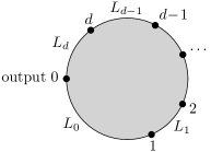
  Figure 1.2. A disc with boundary punctures, showing the ordering convention in the definition of the Fukaya $A_{\infty}$-operation $\mu^{d}(a_{1},\dots,a_{d})$.

• We write $\mathit{HH}_{*}(\mathcal{A})$, $\mathit{HH}^{*}(\mathcal{A})$, $\mathit{HC}_{*}(\mathcal{A})$, $\mathit{HP}_{*}(\mathcal{A})$ for, respectively, Hochschild homology, Hochschild cohomology, negative, and periodic cyclic homology (note that in spite of the subscript, the grading on Hochschild and cyclic homology is still cohomological). The notation for the underlying standard chain complexes is $C_{*}(\mathcal{A})$, $C^{*}(\mathcal{A})$, $\mathit{CC}_{*}(\mathcal{A})$, and lastly $\mathit{CC}_{*}(\mathcal{A})\otimes_{{\mathbb{K}}[u]}{\mathbb{K}}[u^{\pm 1}]$; we’ll actually use several variants of those complexes, and the notation will be slightly modified accordingly.

• The formal variable $u$ which appears in $S^{1}$-equivariant Floer cohomology and in cyclic homology agrees with the convention in [38], meaning that the sign is opposite of that in [34, 80]; see [80, Remark 3.19]. This choice of sign is already visible in the definition of the quantum connection, compare (1.2.3) and [34, Definition 3.1].

• On a symplectic manifold $(M,\omega_{M})$, the Hamiltonian vector field $X$ of a function $H$ satisfies $\omega_{M}(\cdot,X)=dH$. The Poisson bracket is $\{H_{1},H_{2}\}=-\omega_{M}(X_{1},X_{2})$.

• In the context of Floer cohomology, or more generally Cauchy-Riemann equations for maps $u:S\rightarrow M$, we use the following notation. $(S,j_{S})$ is a Riemann surface; $J_{S}$ is a family of almost complex structures on $M$ parametrized by $S$; and $K_{S}$ is a one-form on $S$ with values in $C^{\infty}(M,{\mathbb{R}})$, which is used to define the inhomogeneous term $Y_{S}$ in the Cauchy-Riemann equation, see (4.1.1). If $S$ has boundary, the boundary conditions $L_{S}$ are a family of Lagrangian submanifolds of $M$ parametrized by points of $\partial S$. For Hamiltonian Floer cohomology, which lives on a cylinder $S={\mathbb{R}}\times S^{1}$, we follow the usual convention that $S^{1}={\mathbb{R}}/{\mathbb{Z}}$.

• Operations in Floer cohomology are defined using a variety of parameter spaces (moduli spaces) of Riemann surfaces, the main ones of which are listed in Figure 1.3.

notation	objects parametrized	algebraic operation
$\mathfrak{F}_{m}$	points in the plane (Fulton-MacPherson); Section 5.2a	$\ell^{m}$ and $\delta_{q}^{\mathit{diag}}$; Sections 5.3a, 5.3e
$\mathfrak{C}_{m}$	points on the cylinder; Section 5.2b	$\ell^{m,1}$ and $\delta_{q}$; Sections 5.3b, 5.3e
$\mathfrak{A}_{r}$	cylinders with angles; Section 5.2c	$\delta_{S^{1}}$; Section 5.3c
$\mathfrak{AC}_{m,r}$	cylinders with angles and points; Section 5.2d	$\ell^{m,1}_{S^{1}}$ and $\delta_{S^{1},q}$; Sections 5.3d, 5.3e
$\mathfrak{AC}_{m,r,w}^{(A)}$, $\mathfrak{AC}_{m,r,w}^{(B)}$	same as before, but with constraints on one interior marked point; Sections 5.2e–5.2f	$KH_{(A)}$, $KH_{(B)}$; Section 5.3f
$\mathfrak{R}_{d}$	points on the boundary of the disc (Fukaya-Stasheff); Section 6.1a	$\mu^{d}$; Section 6.2a
$\mathfrak{R}_{d,m}$	discs with boundary and interior marked points; Section 6.1c	$\mu_{q}^{d}$; Section 6.2b
$\mathfrak{R}_{d,m}^{\pm}$, $\mathfrak{R}_{d,m}^{0}$	same as before, but with constraints on one of the interior points; Section 6.3a	$GM_{\pm}$, $GM_{0}$; Section 6.3a
$\mathfrak{AH}_{d,m,r}$	half-cylinders with angles and points; Section 6.1e	plays an auxiliary role, to define the spaces below
$\mathfrak{AH}_{d,m,r}^{(1)}$, $\mathfrak{AH}_{d,m,r}^{(2)}$	subsets of $\mathfrak{AH}_{d,m,r}$; Sections 6.1f–6.1g	$\mathit{OC}_{S^{1},q,(1)}$, $\mathit{OC}_{S^{1},q,(2)}$; Section 6.2d
$\mathfrak{AH}_{d,m,r,w}^{(A1)}$ etc.	same as before, but with constraints on one interior marked point; Sections 6.3c–6.3f	$\mathit{IT}_{(A1)}$ etc. Sections 6.3c–6.3f

Figure 1.3. Notation for the most relevant moduli spaces of Riemann surfaces, and the Floer-theoretic operations they give rise to.

Acknowledgements. The idea of Fourier-Laplace transform, as applied to $S^{1}$-equivariant symplectic cohomology, was first mentioned to the second author by Nicholas Sheridan. We thank Kai Hugtenburg and Claude Sabbah for very useful explanations of their work. Both authors were partially funded by the Simons Collaboration in Homological Mirror Symmetry (Simons Foundation award 652299). The first author additionally received partial funding from NSF grant DMS-2306204. The second author additionally received partial funding as a Simons Investigator (Simons Foundation award 256290); from NSF grant DMS-1904997; and during a visit to the Simons-Laufer Mathematical Sciences Institute, from NSF grant DMS-1928930.

2. Algebraic differential equations

The first aim of this section is to situate our statements in the context of the classical algebraic theory of linear differential equations, of which a rather selective account is given in Section 2.1 (see [55]; the authors have found [68, Ch. II and V] to be a helpful introduction to the subject). This is followed by a short digression on Gauss-Manin connections in algebraic geometry, Section 2.2, which is not necessary for our purpose, but may provide some helpful intuition. Finally, in Section 2.3, we do some preliminary work that’s required for the noncommutative geometry version of the Gauss-Manin connection.

2.1. Classical theory

2.1a. Formal classification of singularities

The simplest aspect of the theory of algebraic connections is the formal (in the sense of Laurent series) one. One considers

(2.1.1) $$\nabla_{\partial_{q}}=\partial_{q}+A_{q},\;\;\text{ where }\;\;A_{q}=\sum_{k=m}^{\infty}A_{k}q^{k}\in\mathit{Mat}_{r}({\mathbb{C}}((q))).$$

Such connections are acted on by formal gauge transformations $G_{q}\in\mathit{GL}_{r}({\mathbb{C}}((q))$:

(2.1.2) $$\tilde{\nabla}_{\partial_{q}}=G_{q}^{-1}\nabla_{\partial_{q}}G_{q}=\partial_{q}+\tilde{A}_{q},\;\;\text{ where }\tilde{A}_{q}=G_{q}^{-1}A_{q}G_{q}+G_{q}^{-1}(\partial_{q}G_{q}).$$

Occasionally, we will also use the subgroup

(2.1.3) $$I+q\mathit{Mat}_{r}({\mathbb{C}}[[q]])\subset\mathit{GL}_{r}({\mathbb{C}}((q))$$

of gauge transformations which have no poles and constant term equal to the identity. The formal classification of connections is completely understood (for expositions see e.g. [55, Sections II.5 and III.1], [68, Sections II.2 and II.5], or [6]). We will only use a small part of that theory, covering the simplest three classes: nonsingular connections; ones with a regular singular point; and singularities of unramified exponential type.

Definition 2.1.1.

One says that $\nabla_{\partial_{q}}$ is nonsingular if, by a formal gauge transformation, it can be brought into a form where $\tilde{A}_{q}\in\mathit{Mat}_{r}({\mathbb{C}}[[q]])$.

This means that any apparent pole can be transformed away. After that, one can formally integrate to trivialize the connection:

Lemma 2.1.2.

Every connection without a pole, meaning with $m=0$ in (2.1.1), is equivalent by a gauge transformation in (2.1.3) to the trivial one, $\tilde{A}_{q}=0$.

Definition 2.1.3.

$\nabla_{\partial_{q}}$ has a regular singular point if, by a formal gauge transformation, it can be transformed into $\tilde{A}_{q}\in q^{-1}\mathit{Mat}_{r}({\mathbb{C}}[[q]])$.

This means that while the apparent pole order may be higher, it can be reduced to $\leq 1$. (In our terminology, “regular singular point” includes nonsingular connections.) One can then further simplify the situation using the following classical fact:

Lemma 2.1.4.

(i) Every connection with a simple pole, meaning with $m=-1$ in (2.1.1), is formally gauge equivalent to one of the form $\tilde{A}_{q}=q^{-1}\tilde{A}_{-1}$, $\tilde{A}_{-1}\in\mathit{Mat}_{r}({\mathbb{C}})$. For such connections $\tilde{\nabla}_{\partial_{q}}$, the formal gauge equivalence class is completely determined by the conjugacy class of the monodromy

(2.1.4) $$\exp(-2\pi i\tilde{A}_{-1})\in\mathit{GL}_{r}({\mathbb{C}}).$$

This monodromy has the same eigenvalues as $\exp(-2\pi iA_{-1})$, where $A_{-1}$ is the residue of the original connection. (More precisely, $\exp(-2\pi iA_{-1})$ is contained in the closure of the conjugacy class of the monodromy.)

(ii) In the “nonresonant case” where no two eigenvalues of $A_{-1}$ differ by a nonzero integer, one can achieve the same outcome with the sharper condition that $\tilde{A}_{-1}=A_{-1}$, by using a gauge transformation in (2.1.3). In particular, the monodromy is conjugate to $\exp(-2\pi iA_{-1})$.

For higher order poles, one has the elementary splitting lemma (the first part is [88, Chapter IV, Theorem 11.1]; the second part was pointed out to the authors by Hugtenburg):

Lemma 2.1.5.

(i) Take a connection (2.1.1), with $m\leq-2$. This is always equivalent, by a gauge transformation in (2.1.3), to some $\tilde{A}_{q}=\tilde{A}_{m}q^{m}+\tilde{A}_{m+1}q^{m+1}+\cdots$, where $\tilde{A}_{m}=A_{m}$, and the higher order terms preserve the splitting of ${\mathbb{C}}^{r}$ into generalized $A_{m}$-eigenspaces.

(ii) Suppose that $\lambda$ is an eigenvalue of $A_{m}$ such that the $\lambda$-Jordan block is diagonal (no nilpotent part). Then, the associated piece of $\tilde{A}_{m+1}$ is just the block diagonal part of $A_{m+1}$, with respect to the decomposition into generalized eigenspaces. In formulae, if $P_{\lambda}$ is the projection to the generalized $\lambda$-eigenspace, then $P_{\lambda}\tilde{A}_{m+1}P_{\lambda}=P_{\lambda}A_{m+1}P_{\lambda}$.

Definition 2.1.6.

$\nabla_{\partial_{q}}$ has a singularity of unramified exponential type (see [70, Section 2.c] or [72, Lecture 1]) if it can be formally gauge transformed into a direct sum

(2.1.5) $$\tilde{\nabla}_{\partial_{q}}=\bigoplus_{\lambda}\tilde{\nabla}_{\partial_{q},\lambda},\qquad\tilde{\nabla}_{\partial_{q},\lambda}=\tilde{\nabla}_{\partial_{q},\lambda}^{\mathrm{reg}}+\lambda q^{-2}I,$$

where the $\lambda$ are a finite set of complex numbes, and each $\tilde{\nabla}_{\partial_{q},\lambda}^{\mathrm{reg}}$ has a regular singular point. The monodromies of the $\tilde{\nabla}_{\partial_{q},\lambda}^{\mathrm{reg}}$ will be called the regularized formal monodromies of $\nabla_{\partial_{q}}$.

(In our terminology, “unramified exponential type” includes connections with a regular singular point as the special case where there is only one summand, with $\lambda=0$.) One can think of $\tilde{\nabla}_{\partial_{q},\lambda}$ as the tensor product of the scalar (rank $1$) connection $\partial_{q}+\lambda q^{-2}$ and of $\tilde{\nabla}_{\partial_{q},\lambda}^{\mathrm{reg}}$; the latter part can then be further simplified by applying Lemma 2.1.4. The decomposition (2.1.5) is essentially unique, which means that the $\lambda$ and the formal gauge equivalence class of each $\tilde{\nabla}_{\partial_{q},\lambda}^{\mathrm{reg}}$ are invariants of the original connection; this is a consequence of the Hukuhara-Turrittin-Levelt theorem (see e.g. [54, Théorème 2.1]). As a consequence, the conjugacy classes of the regularized formal monodromies are gauge invariants of the original connection $\nabla_{q}$.

Lemma 2.1.7.

(i) Suppose that $A_{q}$ has a quadratic pole, meaning that $m=-2$ in (2.1.1), and has unramified exponential type. Then the numbers $\lambda$ that appear in (2.1.5) are the eigenvalues of $A_{-2}$, and the dimension of each summand is the multiplicity of that eigenvalue.

(ii) Suppose that $A_{q}$ has a quadratic pole, and that $A_{-2}$ is semisimple. Then the connection has unramified exponential type, and can be brought into the form (2.1.5) by a gauge transformation without poles. Moreover, the regularized formal monodromy of each summand has the same eigenvalues as $\exp(-2\pi iA_{-1,\lambda})$, where $A_{-1,\lambda}$ are the block diagonal terms one gets when decomposing $A_{-1}$ acconding to the eigenspaces of $A_{-2}$.

Both statements are well-known (for (i) see e.g. see [73, Corollary 3.2], and for the main part of (ii) see [70, Example 2.6]). The proof essentially uses only Lemma 2.1.5.

Remark 2.1.8.

The dual of a connection $\nabla_{\partial_{q}}=\partial_{q}+A_{q}$ is $\nabla^{*}_{\partial_{q}}=d-A_{q}^{\mathrm{tr}}$ (note we are not using complex conjugation here). By dualizing gauge transformations, one sees that $\nabla_{\partial_{q}}^{*}$ has unramified exponential type if and only if $\nabla_{\partial_{q}}$ does; the corresponding numbers are related by $\lambda^{*}=-\lambda$; and the regularized monodromies of $\nabla^{*}_{\partial_{q}}$ are conjugate to the inverse transposes of those of $\nabla_{\partial_{q}}$.

The global picture is that we consider rational connections on the affine line. Take a nonzero $p\in{\mathbb{C}}[q]$, and write ${\mathbb{C}}[q,1/p]\subset{\mathbb{C}}(q)$ for the subring of rational functions generated by $q$ and $1/p$. A rational connection is of the form

(2.1.6) $$\nabla_{\partial_{q}}=\partial_{q}+A_{q},\;\;\text{ where $A_{q}\in\mathit{Mat}_{r}({\mathbb{C}}[q,1/p])$.}$$

By formally expanding in $(q-\sigma)$ for some $\sigma$, one can define $\sigma$ being a nonsingular point, or a regular singular point, and so on, of the connection (obviously, all $\sigma\in{\mathbb{C}}$ where $p(\sigma)\neq 0$ will be nonsingular points). That also extends to $\sigma=\infty$, by expanding in $Q=1/q$.

2.1b. Application to quantum connections

Let’s see how the general theory works out for quantum connections, starting with simple examples.

Example 2.1.9.

(This is an entirely fictitious consideration, as there are no known monotone symplectic manifolds with that property.) Suppose that there are no Gromov-Witten contributions to the quantum connection, meaning that $[\omega_{M}]\ast^{(k)}x=0$ for all $k>0$, in the notation from (1.1.3). Then, from (1.1.2) or (1.1.6), it’s clear that $q=\infty$ is also a regular singular point. The monodromy around that point is the inverse of that around $q=0$, hence has a unipotent Jordan block of size $\mathrm{dim}_{{\mathbb{C}}}(M)+1$, which would saturate the bound of Theorem 1.3.2.

Example 2.1.10.

The quantum connection on $M={\mathbb{C}}P^{1}$ is

(2.1.7) $$\nabla_{\partial_{q}}=\partial_{q}+\begin{pmatrix}0&2q\\ 2q^{-1}&0\end{pmatrix},$$

where the factors of $2$ come from $[\omega_{M}]=c_{1}(M)=2[\mathit{point}]$. Written as in (1.1.7), it becomes

(2.1.8) $$\nabla_{\partial_{Q}}^{\mathrm{Gr}}=\partial_{Q}-Q^{-2}\begin{pmatrix}0&2\\ 2&0\end{pmatrix}+Q^{-1}\begin{pmatrix}0&0\\ 0&1\end{pmatrix}.$$

Applying the algorithm underlying Lemma 2.1.5, one finds that it is gauge equivalent to

(2.1.9) $$\tilde{\nabla}_{\partial_{Q}}^{\operatorname{gr}}=\partial_{Q}+Q^{-2}\begin{pmatrix}-2&0\\ 0&2\end{pmatrix}+Q^{-1}\begin{pmatrix}{\textstyle\frac{1}{2}}&0\\ 0&{\textstyle\frac{1}{2}}\end{pmatrix}.$$

In words, it is of unramified exponential type, and the regularized formal monodromies of both summands are equal to $-1$. This illustrates the fact that (as a consequence of the Stokes phenomenon) the regularized formal monodromies usually don’t agree with the monodromy of the connection in the classical sense.

Example 2.1.11.

Take the quantum connection on the cubic surface [16, 14], restricted to the invariant subspace spanned by ($1$, the first Chern class, the Poincaré dual of a point). One gets

(2.1.10) $$\nabla_{\partial_{Q}}^{\mathrm{Gr}}=\partial_{Q}-Q^{-2}\begin{pmatrix}0&108&252\\ 1&9&36\\ 0&3&0\end{pmatrix}+Q^{-1}\begin{pmatrix}0&0&0\\ 0&1&0\\ 0&0&2\end{pmatrix}.$$

It turns out (code can be found at [75]) that this is gauge equivalent to

(2.1.11) $$\partial_{Q}-Q^{-2}\begin{pmatrix}-6&0&0\\ 0&-6&0\\ 0&0&21\end{pmatrix}+Q^{-1}\begin{pmatrix}5/3&-40/729&0\\ 0&1/3&0\\ 0&0&1\end{pmatrix}+O(1).$$

By Lemma 2.1.7, this connection is of unramified exponential type. The regularized formal monodromy has eigenvalues $1$ (for the $\lambda=21$ part), respectively the nontrivial third roots of unity (for the $\lambda=-6$ part). To complete the discussion, note that there is a complementary invariant subspace, which is the orthogonal complement of $[\omega_{M}]$ inside $H^{2}(M;{\mathbb{C}})$. On that subspace, $[\omega_{M}]\ast$ acts by $-6$ times the identity; therefore, the corresponding part of $\nabla_{\partial_{Q}}^{\mathit{Gr}}$ has unramified exponential type and trivial regularized monodromy.

Remark 2.1.12.

A twistor construction ([65], see also [21]) associates to each closed hyperbolic $6$-manifold a $12$-dimensional monotone symplectic (but not Kähler) manifold. An unpublished argument of Hugtenburg, based on quantum cohomology computations in [20], shows that the quantum connection for those manifolds has unramified exponential type. (The authors apologize for having wrongly stated the opposite in conference talks.)

We want to record a few observations about the quantum connection in general, which shed light on the computations above. All of them are familiar, and they share a common ingredient, namely Poincaré duality.

Lemma 2.1.13.

The quantum connection is gauge equivalent to its dual (see Remark 2.1.8) up to a parameter change $q\mapsto-q$.

Proof.

Using Poincaré duality, one can write the dual of (1.1.2) as $\nabla_{\partial_{q}}^{*}x=\partial_{q}x-q^{-1}([\omega_{M}]\ast_{q}x)$. Pulling this back by $q\mapsto-q$ yields the connection

(2.1.12) $$\partial_{q}x-q^{-1}([\omega_{M}]\ast_{-q}x).$$

Now take an automorphism $\Phi$ of $H^{*}(M;{\mathbb{C}})$ which in degree $d$ is $\phi_{d}$ times the identity, where $\phi_{d+2}=-\phi_{d}$. This satisfies $\Phi([\omega_{M}]\ast_{-q}x)=-\Phi([\omega_{M}]\ast_{q}x)$, hence turns (2.1.12) back into the quantum connection. ∎

Corollary 2.1.14.

Suppose that $\nabla_{\partial_{Q}}^{\mathrm{Gr}}$ has unramified exponential type. Then, each of the regularized formal monodromies is conjugate to its inverse transpose. Hence, the spectrum of the monodromy must be invariant under $\lambda\leftrightarrow 1/\lambda$.

Lemma 2.1.15.

Suppose that $\lambda$ is an eigenvalue of $[\omega_{M}]\ast$, which is simple (the associated generalized eigenspace is one-dimensional). Then, the corresponding piece of the quantum connection, in the sense of Lemma 2.1.5, is of unramified exponential type, and has regularized monodromy $(-1)^{\mathrm{dim}_{\mathbb{C}}(M)}$.

Proof.

The first statement (unramified exponential type) is obvious from Lemma 2.1.5(i). As for the second one, write $H_{\lambda}$ for the eigenspace in question. Any such space is itself a ${\mathbb{Z}}/2$-graded commutative unital ring. As a consequence, a one-dimensional eigenspace must be contained in $H^{\operatorname{even}}(M;{\mathbb{C}})$. To simplify computations, assume that $\mathrm{Gr}|H^{d}(M;{\mathbb{C}})$ is $d$ times the identity for even $d$. Write $H_{\lambda}^{\perp}$ for the direct sum of all other generalized eigenspaces in $H^{\operatorname{even}}(M;{\mathbb{C}})$. The notation is explained by the fact that these two spaces are orthogonal for the intersection pairing. As a consequence, the intersection pairing is nonzero when restricted to $H_{\lambda}$. Next, note that $\mathrm{Gr}-\mathrm{dim}_{{\mathbb{C}}}(M)\,I$ is skewadjoint for the intersection pairing. In particular,

(2.1.13) $$\int_{M}\mathrm{Gr}(x)x=\mathrm{dim}_{{\mathbb{C}}}(M)\int_{M}x^{2}.$$

When applied to $x\in H_{\lambda}$, this tells us that the first block diagonal entry of $\mathrm{Gr}$ with respect to the decomposition $H_{\operatorname{even}}(M;{\mathbb{C}})=H_{\lambda}\oplus H_{\lambda}^{\perp}$ is equal to $\mathrm{dim}_{{\mathbb{C}}}(M)$. One now applies Lemma 2.1.5(ii). ∎

The following generalization of Lemma 2.1.15 comes from Dubrovin’s work [19, Lecture 3] (see [28, Section 2.4] for an exposition in a language close to the one here; ours is a simplified version of their statement).

Lemma 2.1.16.

If the quantum cohomology ring $(H^{*}(M),\ast)$ is semisimple (the direct sum of copies of ${\mathbb{C}}$), then the quantum connection has unramified exponential type, and $(-1)^{\mathrm{dim}_{\mathbb{C}}(M)}$ is the only eigenvalue of the regularized monodromies.

Proof.

Unramified exponential type is obvious from Lemma 2.1.7. In this case there can be no odd degree cohomology. We assume that $\mathrm{Gr}$ is as in the proof of Lemma 2.1.15. Write $\langle x_{1},\dots,x_{n}\rangle$ for $n$-pointed genus zero Gromov-Witten invariants, so that

(2.1.14) $$\int_{M}(x_{1}\ast x_{2})x_{3}=\langle x_{1},x_{2},x_{3}\rangle.$$

As a special case of the divisor axiom,

(2.1.15) $$2\langle c_{1}(M),x_{1},x_{2},x_{3}\rangle+\int_{M}\mathrm{Gr}(x_{1}\ast x_{2})x_{3}=\int_{M}(\mathrm{Gr}(x_{1})\ast x_{2}+x_{1}\ast\mathrm{Gr}(x_{2}))x_{3}.$$

The five-point WDVV relation is

(2.1.16) $$\langle x_{1}\ast x_{2},x_{3},x_{4},x_{5}\rangle+\langle x_{1},x_{2},x_{3}\ast x_{4},x_{5}\rangle=\langle x_{1}\ast x_{3},x_{2},x_{4},x_{5}\rangle+\langle x_{1},x_{3},x_{2}\ast x_{4},x_{5}\rangle.$$

In our situation, there is a basis $\{e_{i}\}$ of idempotents for the quantum product. These satisfy $e_{i}\ast e_{j}=0$ and hence also $\int_{M}e_{i}e_{j}=0$ for $i\neq j$. Moreover, $c_{1}(M)\ast e_{i}=\lambda_{i}e_{i}$ for some $\lambda_{i}\in{\mathbb{C}}$. Applying (2.1.15) yields

(2.1.17) $$\text{for $e_{i}\neq e_{j}$, }\;\;2\langle c_{1}(M),e_{i},e_{j},e_{j}\rangle=2\langle c_{1}(M),e_{i},e_{j},e_{j}\rangle+\int_{M}\mathrm{Gr}(e_{i}\ast e_{j})e_{j}=$$

$$\quad=\int_{M}(\mathrm{Gr}(e_{i})\ast e_{j}+e_{i}\ast\mathrm{Gr}(e_{j}))e_{j}=\int_{M}(\mathrm{Gr}(e_{i})\ast e_{j}+e_{i}\ast\mathrm{Gr}(e_{j}))\ast e_{j}$$

$$\quad=\int_{M}\mathrm{Gr}(e_{i})\ast e_{j}=\int_{M}\mathrm{Gr}(e_{i})e_{j}.$$

From (2.1.16) for $(x_{1},\dots,x_{5})=(c_{1}(M),e_{i},e_{j},e_{j},e_{j})$ one gets

(2.1.18) $$\text{for $e_{i}\neq e_{j}$, }\;\;\langle c_{1}(M),e_{i},e_{j},e_{j}\rangle=(\lambda_{j}-\lambda_{i})\langle e_{i},e_{j},e_{j},e_{j}\rangle.$$

As a consequence of (2.1.13), (2.1.17) and (2.1.18) one sees that

(2.1.19) $$\text{if $\lambda_{i}=\lambda_{j}$, then}\;\;\int_{M}\mathrm{Gr}(e_{i})e_{j}=\begin{cases}\mathrm{dim}_{{\mathbb{C}}}(M)\int_{M}e_{i}^{2}&i=j,\\ 0&i\neq j.\end{cases}$$

In other words, each block diagonal part of $\mathrm{Gr}$ with respect to the decomposition into eigenspaces is $\mathrm{dim}_{{\mathbb{C}}}(M)$ times the identity. One applies Lemma 2.1.7(ii) to obtain the desired conclusion. ∎

2.1c. Differential operators

An alternative viewpoint on the formal classification of connections is provided by the cyclic vector lemma, which says that there is some $v\in{\mathbb{C}}((q))^{r}$ such that $v,\nabla_{\partial_{q}}v,\dots,\nabla_{\partial_{q}}^{r-1}v$ form a basis. The connection gauge transformed to that basis has the form

(2.1.20) $$\partial_{q}+\begin{pmatrix}&&&&-a_{0}\\ 1&&&&-a_{1}\\ &1&&&-a_{2}\\ &&\cdots&&\cdots\\ &&&1&-a_{r-1}\end{pmatrix}$$

for $a_{0},\dots,a_{r-1}\in{\mathbb{C}}((q))$. In other words, setting $a_{r}=1$, we have a relation $\sum_{i=0}^{r}a_{i}\nabla_{\partial_{q}}^{i}v=0$. We correspondingly define an order $r$ scalar differential operator

(2.1.21) $$P_{q}=\sum_{i=0}^{r}a_{i}\partial_{q}^{i}.$$

Suppose that $w\in{\mathbb{C}}((q))^{r}$ is a covariantly constant section of the dual connection, $(\partial_{q}-A_{q}^{\mathrm{tr}})w=0$. Then, the function $f=v\cdot w\in{\mathbb{C}}((q))$ solves $P_{q}f=0$.

Remark 2.1.17.

For the quantum connection, each class $y\in H^{*}(M;{\mathbb{C}})$ gives rise to a covariantly constant section $\Psi_{y}$ of the (Poincaré) dual connection [42, Section 28.1]. These fundamental solutions are generally multivalued, meaning that they have coefficients in ${\mathbb{C}}[\log(q)]((q))$ (which makes sense since there’s an obvious action of $\partial_{q}$ on that ring). Explicitly,

(2.1.22) $$\int_{M}x\Psi_{y}=\int_{M}xe^{\log(q)[\omega_{M}]}y+\sum_{\begin{subarray}{c}d>0\\ m\geq 0\end{subarray}}q^{d}\big{\langle}x,\psi^{m}(e^{\log(q)[\omega_{M}]}y)\big{\rangle}_{d}.$$

Here, we use standard notation $\langle x_{1},\psi^{m}(x_{2})\rangle_{d}$ for two-pointed Gromov-Witten invariants with gravitational descendants, counting rational curves with first Chern number $d$. The covariant constancy property can be expressed as

(2.1.23) $$\partial_{q}\int_{M}x\Psi_{y}=\int_{M}(\nabla_{\partial_{q}}x)\Psi_{y}.$$

As discussed above, if $v$ is a cyclic vector and $P_{q}$ the resulting operator, then

(2.1.24) $$P_{q}\big{(}\textstyle\int_{M}v\Psi_{y}\big{)}=0\;\;\text{for all $y$.}$$

Remark 2.1.18.

Instead of considering the entire quantum connection, let’s just look at the ${\mathbb{C}}((q))$-linear subspace spanned by $1\in H^{0}(M)$ and its $\nabla_{\partial_{q}}$-derivatives, so that $v=1$ is tautologically a cyclic vector. Let $P_{q}$ be the associated differential operator. The analogue of (2.1.24) is that

(2.1.25) $$P_{q}(J_{y})=0,$$

where we write (using the string equation)

(2.1.26) $$J_{y}=\int_{M}\Psi_{y}=\int_{M}e^{\log(q)[\omega_{M}]}y+\sum_{\begin{subarray}{c}d>0\\ m>0\end{subarray}}q^{d}\langle\psi^{m-1}(e^{\log(q)[\omega_{M}]}y)\rangle.$$

In Givental’s terminology (see e.g. [15, Section 10.3] for an exposition in the proper context, which is more general than the one here), a differential operator $\tilde{P}_{q}=\sum_{i}\tilde{a}_{i}\partial_{q}^{i}$, $\tilde{a}_{i}\in{\mathbb{C}}((q))$, is called a quantum differential operator if it satisfies the analogue of (2.1.25), meaning that

(2.1.27) $$\tilde{P}_{q}(J_{y})=0\text{ for all $y$}\;\;\Leftrightarrow\int_{M}(\sum_{i}\tilde{a}_{i}\nabla_{\partial_{q}}^{i}(1))\cdot\Psi_{y}=0\text{ for all $y$}\;\;\Leftrightarrow\;\;\sum_{i}\tilde{a}_{i}\nabla_{\partial_{q}}^{i}(1)=0.$$

Because the definition of $P_{q}$ involves the lowest degree relation between the $\nabla_{\partial_{q}}^{i}(1)$, we then have $\tilde{P}_{q}=(\text{\it some differential operator})P_{q}$; in terms of the Weyl algebra to be introduced in a little while, the quantum differential operators are the left ideal generated by $P_{q}$. By an easy degree argument, the rightmost equation in (2.1.27) implies the following: if the coefficients $\tilde{a}_{i}$ of only contain powers $q^{k}$ of less, the relation

(2.1.28) $$\sum_{i=0}^{r}\text{($q^{k}$-term of $\tilde{a}_{i}$)}[\omega_{M}]^{\ast i}=0$$

holds in quantum cohomology (compare [15, Theorem 10.3.1]).

The Newton polygon of $P_{q}$ is constructed as follows. For each $0\leq i\leq r$ such that $a_{i}\neq 0$, take the point $(x_{i},y_{i})=(i,\mathrm{val}_{q}(a_{i})-i)$, where $\mathrm{val}_{q}(a_{i})$ is the lowest power of $q$ which occurs. Consider the subsets

(2.1.29) $$\{0\leq x\leq x_{i},\;y\geq y_{i}\}.$$

The Newton polygon is the convex hull of the union of those subsets. The slopes of $P_{q}$ are the finite (meaning, excluding vertical sides) slopes of the sides of the Newton polygon. These slopes are nonnegative rational numbers, and are invariants of the original connection (which means, they are independent of the choice of cyclic vector $v$; see e.g. [55, Theorem III.1.5]). The classical Fuchs regularity criterion is:

Lemma 2.1.19.

$\nabla_{\partial_{q}}$ has a regular singular point if and only if $0$ is the only slope of $P_{q}$.

More generally, the slopes describe the pole orders of the pieces of the Hukuhara-Turrittin-Levelt decomposition of a connection [87, Remark 3.55]. As a special case, one has:

Lemma 2.1.20.

If $\nabla_{\partial_{q}}$ has a singularity of unramified exponential type, the slopes of $P_{q}$ are a subset of $\{0,1\}$.

Example 2.1.21.

Consider [49, Remark 2.13]

(2.1.30) $$A_{q}=\begin{pmatrix}0&-q^{-2}\\ -q^{-1}&-{\textstyle\frac{1}{2}}q^{-1}\end{pmatrix}.$$

The cyclic vector $v=(1,0)$ yields a differential operator with slope $1/2$,

(2.1.31) $$P_{q}=\partial_{q}^{2}+{\textstyle\frac{3}{2}}q^{-1}\partial_{q}-q^{-3}.$$

Hence, this is not of unramified exponential type. One can also see this in a different way (following the argument in [49]). Namely, introducing a square root $q^{1/2}$ allows the gauge transformation

(2.1.32) $$G_{q}=\begin{pmatrix}1&1\\ -q^{1/2}&q^{1/2}\end{pmatrix}\;\;\Longrightarrow\;\;\tilde{A}_{q}=q^{-3/2}\begin{pmatrix}1&0\\ 0&-1\end{pmatrix}.$$

By the uniqueness part of the Hukuhara-Turrittin-Levelt theorem, this rules out unramified exponential type.

Example 2.1.22.

Take the previous example, and add $q^{-2}$ times the identity matrix to $A_{q}$. For the same cyclic vector, one now gets

(2.1.33) $$\textstyle P_{q}=\partial_{q}^{2}+(\frac{3}{2}q^{-1}-2q^{-2})\partial_{q}+(q^{-4}-{\textstyle\frac{1}{2}}q^{-3}),$$

whose only slope is $1$. However, this connection is still not of unramified exponential type, since by (2.1.32) it’s gauge equivalent to $\tilde{A}_{q}=(q^{-2}+q^{-3/2})I$. This shows that the converse to Lemma 2.1.20 is false.

2.1d. Fourier-Laplace transform

Let $W_{q}$ be the Weyl algebra of differential operators in one variable $q$, over ${\mathbb{C}}$. This is generated by $q$ and $\partial_{q}$, with the relation

(2.1.34) $$[\partial_{q},q]=1.$$

Left $W_{q}$-modules are called $D$-modules. If $N_{q}$ is a $D$-module, and $p\in{\mathbb{C}}[q]$ is nonzero,

(2.1.35) $$N_{q,1/p}\stackrel{{\scriptstyle\mathrm{def}}}{{=}}{\mathbb{C}}[q,1/p]\otimes_{{\mathbb{C}}[q]}N_{q}$$

inherits the structure of a $D$-module (by the obvious differentiation rule). A $D$-module $N_{q}$ is called holonomic if it is finitely generated and, for every $x\in N_{q}$, there is a nonzero $w\in W_{q}$ such that $wx=0$. If $N_{q}$ is holonomic, then so are its localisations (2.1.35). Given a rational connection $\nabla_{\partial_{q}}$ as in (2.1.6), the space ${\mathbb{C}}[q,1/p]^{r}$, with $\partial_{q}$ acting by $\nabla_{\partial_{q}}$, becomes a holonomic $D$-module. The $W_{q}$-modules obtained in this way are precisely those on which $p$ acts invertibly, and which are finitely generated over ${\mathbb{C}}[q,1/p]$ (freeness over ${\mathbb{C}}[q,1/p]$ is then an automatic consequence). In the converse direction, one has (see e.g. [68, p. 171]):

Lemma 2.1.23.

Let $N_{q}$ be a holonomic $D$-module. Then there is a nonzero $p\in{\mathbb{C}}[q]$, such that $N_{q,1/p}$ is isomorphic to the $D$-module coming from a connection (2.1.6).

Take a minimal such $p$. One calls $\Sigma_{q}=p^{-1}(0)$ the set of singularities of the $D$-module $N_{q}$, and speaks of the associated rational connection $\nabla_{\partial_{q}}$ (which, in our formulation, is unique up to gauge equivalence over ${\mathbb{C}}\setminus\Sigma_{q}$).

Definition 2.1.24.

Let $t$ be another formal variable. We identify $W_{t}\cong W_{q}$ by setting

(2.1.36) $$t=\partial_{q},\;\;\partial_{t}=-q.$$

Given a $W_{t}$-module $N_{t}$, the Fourier-Laplace transform $N_{q}$ is simply the same space considered as a module over $W_{q}$ via (2.1.36). This clearly preserves holonomicity.

Example 2.1.25.

Take linear maps $U:{\mathbb{C}}^{r}\rightarrow{\mathbb{C}}^{s}$, $V:{\mathbb{C}}^{s}\rightarrow{\mathbb{C}}^{r}$, as well as some $\sigma\in{\mathbb{C}}$. Define a holonomic $D$-module

(2.1.37) $$N_{t}={\mathbb{C}}[t]^{r}\oplus{\mathbb{C}}[\partial_{t}]^{s},$$

with the $W_{t}$-action

(2.1.38) $$\partial_{t}(t^{m}x,\partial_{t}^{n}y)=(mt^{m-1}x,\partial_{t}^{n+1}y)+\begin{cases}(t^{m-1}VUx,0)&m>0,\\ (0,Ux)&m=0;\end{cases}$$

$$t(t^{m}x,\partial_{t}^{n}y)=(t^{m+1}x,\sigma\partial_{t}^{n}y-n\partial_{t}^{n-1}y)+\begin{cases}(0,\partial_{t}^{n-1}UVy)&n>0,\\ (Vy,0)&n=0.\end{cases}$$

Any element of the second summand of (2.1.37) is mapped to the first summand by a sufficiently high power of $(t-\sigma)$; and $(t-\sigma)\partial_{t}(x,0)=(VUx,0)$. From that, one sees that $N_{t,1/(t-\sigma)}$ is the module associated to the connection

(2.1.39) $$\nabla_{t}=\partial_{t}+(t-\sigma)^{-1}VU.$$

Apply the Fourier-Laplace transform, and write the summands in the opposite order, which means as $N_{q}={\mathbb{C}}[q]^{s}\oplus{\mathbb{C}}[\partial_{q}]^{r}$. Then, $N_{q,1/q}$ is the module associated to $\nabla_{\partial_{q}}=\partial_{q}-q^{-1}UV+\sigma$. Changing coordinates to $Q=1/q$ yields

(2.1.40) $$\nabla_{\partial_{q}}=\partial_{Q}-Q^{-2}\sigma+Q^{-1}UV.$$

Remark 2.1.26.

Take $P_{q}\in W_{q}$ and a formal power series solution, meaning some $\Pi=\sum_{m=0}^{\infty}a_{m}q^{m}\in{\mathbb{C}}[[q]]$ such that $P_{q}\Pi=0$. Then

(2.1.41) $$\hat{\Pi}\stackrel{{\scriptstyle\mathrm{def}}}{{=}}\sum_{m=0}^{\infty}m!a_{m}t^{-m-1}\in t^{-1}{\mathbb{C}}[[t^{-1}]]$$

is a formal solution of the dual equation $P_{t}\hat{\Pi}=0$, where $P_{t}$ corresponds to $P_{q}$ under (2.1.36). In the case of the quantum connection and the setting from Remark 2.1.18, the quantum period is defined to be (2.1.26) specialized to the class $y=p$ Poincaré dual to a point,

(2.1.42) $$\Pi=J_{p}=1+\sum_{d\geq 2}q^{d}\langle\psi^{d-2}(p)\rangle_{d}.$$

Then $\hat{\Pi}$ is essentially the regularized quantum period (see e.g. [12] for the terminology).

The general relation between a holonomic $D$-module and its Fourier-Laplace transform was studied extensively in [55]. We will need only a special case of the results from [55, Ch. IX-XI]:

Proposition 2.1.27.

Let $N_{t}$ be a holonomic $W_{t}$-module, with singularities at $\Sigma_{t}\subset{\mathbb{C}}$. Suppose that the associated rational connection $\nabla_{t}$, in the sense of Lemma 2.1.23, has only regular singular points, including at $t=\infty$. Then,

(i) The Fourier-Laplace tranform $N_{q}$ is nonsingular on ${\mathbb{C}}^{*}$. If we look at the associated connection $\nabla_{\partial_{q}}$, then that has a regular singular point at $q=0$, and a singularity of unramified exponential type at $q=\infty$.

(ii) To describe the latter singularity more precisely, let’s change coordinates to $Q=1/q$, and look at the normal form $\tilde{\nabla}_{\partial_{Q}}$ from (2.1.5). The numbers that appear there are precisely $\lambda=-\sigma$ for $\sigma\in\Sigma_{t}$. Moreover, for each $\sigma$ there are there are matrices $U_{\sigma}$, $V_{\sigma}$ such that the monodromy of $\nabla_{t}$ around $\sigma$ is $\exp(-2\pi iV_{\sigma}U_{\sigma})$, and the corresponding regularized formal monodromy around $q=\infty$ (anticlockwise in $Q$, which means clockwise in $q$) is $\exp(-2\pi iU_{\sigma}V_{\sigma})$.

Part (i) is stated for instance in [71, p. 91] or [69, Lemma 1.5]. Part (ii) follows from the fact that the formal structure of $N_{q}$ at $q=\infty$ depends only on the local structure of $N_{t}$ near its singularities [68, Section V.3]. More precisely, every singular point of $N_{t}$ contributes a direct summand to the formal connection $\nabla_{\partial_{q}}$. The local structure of a holonomic $D$-module with a regular singularity at $t=\sigma$ is isomorphic to one of those from Example 2.1.25, see [55, p. 28]; and therefore, the computation carried out in that example actually proves the general result.

Given Proposition 2.1.27(ii), some linear algebra [22] yields the following:

Corollary 2.1.28.

Let $M_{\sigma,\alpha}$ be the monodromy of $\nabla_{t}$ around some singular point $\sigma$, restricted to the generalized $\alpha$-eigenspace; and $N_{\sigma,\alpha}$ the regularized formal monodromy of the $\lambda=-\sigma$ summand of $\tilde{\nabla}_{\partial_{Q}}$, restricted correspondingly.

(i) If $\alpha\neq 1$, $M_{\sigma,\alpha}$ and $N_{\sigma,\alpha}$ are conjugate.

(ii) There is a bijective correspondence between Jordan blocks of $M_{\sigma,1}$ and of $N_{\sigma,1}$, under which sizes change by at most $1$. Here, we think of having an infinite reservoir of size $0$ Jordan blocks on each side, so that size $1$ Jordan blocks can appear and disappear under the correspondence.

2.2. The Gauss-Manin system

2.2a. Definition

Let $X$ be a smooth complex algebraic variety, and $W:X\rightarrow S=\mathbb{A}^{1}$ a proper nonconstant morphism. The Gauss-Manin system is defined [61, Ch. 2, Section 15] as the derived pushforward of the $D$-module sheaf $\mathcal{O}_{X}$ under $W$. To compute it, one factors $W$ as the composition of the embedding $(\mathit{id},W):X\rightarrow X\times S$ and the projection $X\times S\rightarrow S$. Concretely, the outcome is as follows [61, p. 159]. Take the complex of sheaves

(2.2.1) $$\mathcal{E}_{q}=\Omega^{*}_{X}[q],$$

$$d_{\mathcal{E}_{q}}\theta=d\theta-q\,dW\wedge\theta,$$

with the operation

(2.2.2) $$\nabla_{q}(\theta q^{k})=k\theta\,q^{k-1}-W\theta\,q^{k}.$$

The hypercohomology $E_{q}$ of $\mathcal{E}_{q}$ becomes a $W_{q}$-module in each degree. The Gauss-Manin system in degree $k$ is defined as the Fourier-Laplace transform of $E_{q}^{k+1}$. From the general theory (see e.g. [45, Theorem 3.2.3]), one gets:

Lemma 2.2.1.

In each degree, $E_{q}$ is a holonomic $W_{q}$-module.

The picture simplifies away from the singular fibres. Namely, let $S^{\mathrm{reg}}\subset S$ be the set of regular values, and $X^{\mathrm{reg}}=W^{-1}(S^{\mathrm{reg}})$ its preimage. The restriction of the Gauss-Manin system to $S^{\mathrm{reg}}$ can be computed directly using the pushforward by the submersion $W|X^{\mathrm{reg}}$, which yields the classical definition of the Gauss-Manin connection on the hypercohomology of the relative de Rham complex $(\Omega^{*}_{X^{\mathrm{reg}}/S^{\mathrm{reg}}},d)$.

2.2b. Application

In the algebro-geometric context, the counterpart of Conjecture 1.1.1 is:

Proposition 2.2.2.

(i) In each degree, restricting $E_{q}$ to ${\mathbb{C}}^{*}=\{q\neq 0\}$ yields a connection which has a regular singularity at $q=0$, and a singularity of unramified exponential type at $q=\infty$.

(ii) The regularized formal monodromies at $q=\infty$ are quasi-unipotent.

(iii) For each regularized formal monodromy, the spectrum on $E_{q}$ (combining degrees) is invariant under $\lambda\leftrightarrow 1/\lambda$.

Proof.

By the (Griffiths-Landman-Grothendieck) monodromy theorem, the Gauss-Manin connection for $W:X^{\mathrm{reg}}\rightarrow S^{\mathrm{reg}}$ has regular singularities, and quasi-unipotent monodromy around each of those singularities. Moreover, each monodromy endomorphism is compatible with the Poincaré duality pairing on the cohomology of the fibres, and therefore has the same eigenvalues as its inverse. This, together with Lemma 2.2.1, allows us to apply Proposition 2.1.27, which gives the desired result. ∎

Part of enumerative mirror symmetry, as formulated e.g. in [40], is that the Gauss-Manin system of the mirror superpotential should give the quantum connection. In situations where this is proved, one can use Proposition 2.2.2 to derive the corresponding case of Conjecture 1.1.1. Strictly speaking, to use Proposition 2.2.2 as stated, one has to have a proper mirror superpotential, which can be achieved if the mirror is constructed relative to a smooth anticanonical divisor; however, the algebro-geometric considerations can be generalized beyond the proper case, under suitable assumptions on $W$. We had already mentioned one of the results that have been obtained in this way [73].

Example 2.2.3.

The mirror of ${\mathbb{C}}P^{1}$ is the superpotential $X={\mathbb{C}}^{*}$, $W(z)=z+z^{-1}$. The complex (2.2.1) reduces to

(2.2.3)

We have drawn that so as to exhibit an increasing filtration. Using that filtration, one sees that the only nontrivial cohomology group $E_{q}^{1}=H^{1}(\mathcal{E}_{q})$, as a $W_{q}$-module, has generators and relations

(2.2.4) $$a_{0}=[z^{-1}dz],\;\;a_{1}=[dz],$$

$$q\partial_{q}a_{0}=-2qa_{1},$$

$$\partial_{q}qa_{1}=-2qa_{0}.$$

Our module contains $q$-torsion elements: $q[(1-z^{-2})\mathit{dz}]=q(\partial_{q}a_{0}+2a_{1})=0$. If we tensor with ${\mathbb{C}}[q^{\pm 1}]$ and replace the generators with $(a_{0},-qa_{1})$, the relations (2.2.4) yield the quantum connection (2.1.7). Take the Fourier-Laplace transform, and write the relations (2.2.4) as

(2.2.5) $$a_{0}={\textstyle\frac{1}{2}}(t^{2}-4)\partial_{t}a_{1},$$

$$2\partial_{t}a_{0}=-t\partial_{t}a_{1}.$$

After tensoring with ${\mathbb{C}}[t,(t^{2}-4)^{-1}]$, this becomes the connection with

(2.2.6) $$A_{t}=\begin{pmatrix}-\frac{t}{t^{2}-4}&\frac{2}{t^{2}-4}\\ 0&0\end{pmatrix}.$$

As one would expect from its geometric origin, the monodromy around $t=\pm 2$ has eigenvalues $\{-1,1\}$ (it swaps the two sheets of $W$). Via Proposition 2.1.27(ii), that explains the occurrence of the eigenvalues $-1$ in the regularized formal monodromy computation from Example 2.1.10.

Example 2.2.4.

The mirror to the cubic surface (relative to a smooth anticanonical divisor) is obtained from the extremal rational elliptic surface $X_{431}$, in the notation of [57, Theorem 4.1], by removing the $I_{3}$ fibre. More specifically, the base should be parametrized so that the resulting $W:X\rightarrow{\mathbb{C}}$ is a partial compactification of the superpotential given e.g. in [13, Example 10] with a constant $-6$ added (which brings the critical values into their expected position $\{-6,21\}$; for the origin of that constant, see [40, Section 10] and [79, Appendix B]). This $W$ has one nondegenerate singular point, and a more complicated singular fibre which consists of an $\tilde{E}_{6}$ configuration of rational spheres. The monodromy around the last-mentioned fibre has the eigenvalues $\exp(\pm 2\pi i/3)$ seen in Example 2.1.11.

2.3. The noncommutative theory

2.3a. The $(u,q)$-Weyl algebra

(Heisenberg-)Weyl algebras depending on an additional formal variable are of course what occurs in the original quantum mechanics context. In noncommutative geometry the setup is a little different, since the additional formal variable $u$ has degree $2$. As we will not actually be solving any differential equations in this part of our argument, we can work over an arbitrary field ${\mathbb{K}}$.

Let $W_{q,u}$ be the graded ${\mathbb{K}}[u]$-algebra generated by $q$ (of degree $2$) and $u\partial_{q}$ (of degree $0$), with

(2.3.1) $$[u\partial_{q},q]=u.$$

(In spite of the notation, there is no element $\partial_{q}$ in this algebra.) Let’s look at graded (left) modules over $W_{q,u}$, understood to be graded ${\mathbb{K}}[u]$-modules with $u$-linear actions of $q$ and $\partial_{q}$, which satisfy (2.3.1).

• We say that a module is $u$-torsionfree if multiplication by $u$ is injective.

• The $u$-adic completion of a module $A_{q,u}$ (in the graded sense, meaning that we complete in each degree separately) is

  (2.3.2) $$\hat{A}_{q,u}\stackrel{{\scriptstyle\mathrm{def}}}{{=}}\underleftarrow{\lim}_{m}\,A_{q,u}/u^{m}A_{q,u}=\underleftarrow{\lim}_{m}\,\big{(}({\mathbb{K}}[u]/u^{m})\otimes_{{\mathbb{K}}[u]}A_{q,u}\big{)}.$$

  We call $A_{q,u}$ complete if the canonical map $A_{q,u}\rightarrow\hat{A}_{q,u}$ is an isomorphism. (This implies that no nonzero element of $A_{q,u}$ can be divisible by arbitrarily high powers of $u$.) Completions are always complete [1, Lemma 00MC].

• Setting $u=0$ in $A_{q,u}$ yields a module over a graded two-variable polynomial ring, since the actions of $q$ and $u\partial_{q}$ then commute; we denote that by

  (2.3.3) $$A_{q}\stackrel{{\scriptstyle\mathrm{def}}}{{=}}A_{q,u}/uA_{q,u}=({\mathbb{K}}[u]/u)\otimes_{{\mathbb{K}}[u]}A_{q,u}.$$

Just like the notions above, the next Lemmas really concern only the $u$-module structure:

Lemma 2.3.1.

Suppose that $A_{q,u}$ is $u$-torsionfree. Then so is its completion $\hat{A}_{q,u}$. Moreover, the $u=0$ reduction of the completion agrees with that of the original module.

Proof.

We have short exact sequences

(2.3.4) $$0\rightarrow A_{q,u}/u^{m}A_{q,u}\stackrel{{\scriptstyle u}}{{\longrightarrow}}A_{q,u}/u^{m+1}A_{q,u}\longrightarrow A_{q}\rightarrow 0.$$

Passing to the limit (which is exact because the maps that decrease $m$ are surjective) yields

(2.3.5) $$0\rightarrow\hat{A}_{q,u}\stackrel{{\scriptstyle u}}{{\longrightarrow}}\hat{A}_{q,u}\longrightarrow A_{q}\rightarrow 0.$$

∎

Lemma 2.3.2.

Let $A_{q,u}$ and $B_{q,u}$ be complete $u$-torsionfree modules, and $f_{q,u}:A_{q,u}\rightarrow B_{q,u}$ a $W_{q,u}$-linear map whose $u=0$ reduction $f_{q}:A_{q}\rightarrow B_{q}$ is injective. Then $f_{q,u}$ is itself injective, and $C_{q,u}=\mathrm{coker}(f_{q,u})$ is a complete $u$-torsionfree module. Moreover, the $u=0$ reduction $C_{q}$ is the cokernel of $f_{q}$.

Proof.

Injectivity of $f_{q,u}$ is elementary: suppose that $f_{q,u}(a)=0$ for some nonzero $a$. We can write $a=u^{m}a^{\prime}$ with a maximal $m$, and then $f_{q,u}(a^{\prime})=0$, which after reduction to $u=0$ shows that $a^{\prime}$ must again be divisible by $u$, a contradiction. The fact that $C_{q,u}$ is $u$-torsionfree is also elementary: if $uc=0$ in the cokernel, then a lift of $c$ to $b\in B_{q,u}$ would satisfy $ub=f_{q,u}(a)$ for some $a$. This means that the $u=0$ reduction of $a$ lies in the kernel of $f_{q}$, hence must be zero, and we can write $a=ua^{\prime}$. But then $u(b-f_{q,u}(a^{\prime}))=0$, hence $b=f_{q,u}(a^{\prime})$ and $c=0$. At this point, we can tensor with ${\mathbb{K}}[u]/u^{m}$ to get short exact sequences

(2.3.6) $$0\rightarrow A_{q,u}/u^{m}A_{q,u}\stackrel{{\scriptstyle f_{q,u}}}{{\longrightarrow}}B_{q,u}/u^{m}B_{q,u}\longrightarrow C_{q,u}/u^{m}C_{q,u}\rightarrow 0,$$

which for $m=1$ shows the desired fact about $C_{q}$. Passing to the limit $m\rightarrow\infty$ yields

(2.3.7) $$0\rightarrow A_{q,u}\stackrel{{\scriptstyle f_{q,u}}}{{\longrightarrow}}B_{q,u}\longrightarrow\hat{C}_{q,u}\rightarrow 0,$$

which proves that $C_{q,u}=\hat{C}_{q,u}$. ∎

At this point, we add the action of $q$ to the discussion.

• Given a complete module $A_{q,u}$, one can invert $q$ and then take the $u$-completion of that. The outcome of this process will be denoted (slightly clumsily, since the tensor product uses $q$ and the completion uses $u$) by

  (2.3.8) $$A_{q^{\pm 1},u}\stackrel{{\scriptstyle\mathrm{def}}}{{=}}{\mathbb{K}}[q^{\pm 1}]\hat{\otimes}_{{\mathbb{K}}[q]}A_{q,u}.$$

  Here, just like in the framework of classical $D$-modules, the action of $u\partial_{q}$ on the $q$-inverted module is given by $u\partial_{q}(q^{k}\otimes a)=ukq^{k-1}\otimes a+q^{k}\otimes u\partial_{q}a$.

• We write (see Section 1.4(b) for the notation; completion is in the same sense as before)

  (2.3.9) $$q^{-1}A_{q^{-1},u}\stackrel{{\scriptstyle\mathrm{def}}}{{=}}q^{-1}{\mathbb{K}}[q^{-1}]\hat{\otimes}_{{\mathbb{K}}[q]}A_{q,u}.$$

Lemma 2.3.3.

Suppose that $A_{q,u}$ is complete and $u$-torsionfree. Then (2.3.8) is $u$-torsionfree, and its $q=0$ reduction is related to that $A_{q,u}$ in the obvious way:

(2.3.10) $$A_{q^{\pm 1}}\stackrel{{\scriptstyle\mathrm{def}}}{{=}}A_{q^{\pm 1},u}/uA_{q^{\pm 1},u}\cong{\mathbb{K}}[q^{\pm 1}]\otimes_{{\mathbb{K}}[q]}A_{q}.$$

Proof.

Tensoring with ${\mathbb{K}}[q^{\pm 1}]$ yields a short exact sequence

(2.3.11) $$0\rightarrow{\mathbb{K}}[q^{\pm 1}]\otimes_{{\mathbb{K}}[q]}A_{q,u}\stackrel{{\scriptstyle u}}{{\longrightarrow}}{\mathbb{K}}[q^{\pm 1}]\otimes_{{\mathbb{K}}[q]}A_{q,u}\longrightarrow{\mathbb{K}}[q^{\pm 1}]\otimes_{{\mathbb{K}}[q]}A_{q}\rightarrow 0.$$

In words, ${\mathbb{K}}[q^{\pm 1}]\otimes_{{\mathbb{K}}[q]}A_{q,u}$ is $u$-torsionfree, and its $u=0$ reduction is ${\mathbb{K}}[q^{\pm 1}]\otimes_{{\mathbb{K}}[q]}A_{q}$. Lemma 2.3.1 does the rest. ∎

Lemma 2.3.4.

Suppose that $A_{q,u}$ is complete and $u$-torsionfree; and that its $u=0$ reduction $A_{q}$ is $q$-torsionfree ($q$ acts injectively on it). Then (2.3.9) is $u$-torsionfree; its $u=0$ reduction is related to that of $A_{q,u}$ in the obvious way,

(2.3.12) $$q^{-1}A_{q^{-1}}\stackrel{{\scriptstyle\mathrm{def}}}{{=}}q^{-1}A_{q^{-1},u}/uq^{-1}A_{q^{-1},u}\cong q^{-1}{\mathbb{K}}[q^{-1}]\otimes_{{\mathbb{K}}[q]}A_{q};$$

and it fits into a short exact sequence

(2.3.13) $$0\rightarrow A_{q,u}\longrightarrow A_{q^{\pm 1},u}\longrightarrow q^{-1}A_{q^{-1},u}\rightarrow 0.$$

Proof.

Because $A_{q}$ is $q$-torsionfree, so is $A_{q,u}$ (if $x\in A_{q,u}$ satisfies $qx=0$, then it must be a multiple of $u$; that argument can be iterated to prove that $x$ is arbitrarily often $u$-divisible, hence zero by completeness). Therefore, the following diagram has exact columns:

(2.3.14)

The top two rows are exact, hence so is the bottom one. In words, $q^{-1}{\mathbb{K}}[q^{-1}]\otimes_{{\mathbb{K}}[q]}A_{q,u}$ is $u$-torsionfree, and its $u=0$ reduction is $q^{-1}{\mathbb{K}}[q^{-1}]\otimes_{{\mathbb{K}}[q]}A_{q}$. We can then apply Lemma 2.3.1 to carry over those results to $q^{-1}A_{q^{-1}}$. Define (2.3.13) to be the $u$-completion of the left or middle column in (2.3.14). Lemma 2.3.2 tells us that the first map in (2.3.13) is injective. Moreover, concerning the map from its cokernel to $q^{-1}A_{q^{-1},u}$, we then know that its $u=0$ reduction is an isomorphism, which implies that the map itself must be an isomorphism. ∎

Example 2.3.5.

Let $V$ be a graded ${\mathbb{K}}$-vector space. Consider the graded ${\mathbb{K}}[q,u]$-module $A_{q,u}=V[[q,u]]$. Then

(2.3.15) $${\mathbb{K}}[q^{\pm 1}]\otimes_{{\mathbb{K}}[q]}\,A_{q,u}=\underrightarrow{\lim}_{k}\,q^{-k}A_{q,u}=V[[u]]((q))$$

is the space of Laurent series in $q$ with coefficients in $V[[u]]$ (each such Laurent series has a lower bound on the powers of $q$ that can appear). The completion is

(2.3.16) $$A_{q^{\pm 1},u}=V((q))[[u]]=V((q))[[u/q]]$$

which means power series in $u$, or equivalently $u/q$, whose coefficients are Laurent series in $q$. Concretely, an element in (2.3.16) of degree $d$ is a series

(2.3.17) $$\sum_{i\geq 0}\sum_{j\geq m_{i}}(u/q)^{i}q^{j}v_{ij}=\sum_{i\geq 0}\sum_{k\geq m_{i}-i}u^{i}q^{k}v_{i,i+k}$$

for some $m_{i}\in{\mathbb{Z}}$, $v_{ij}\in V^{d-2j}$. In the special case where $V$ is bounded, it follows that $v_{ij}=0$ once $|j|$ exceeds some $d$-dependent bound, and therefore:

(2.3.18) $$A_{q^{\pm 1},u}=(V[[u/q]])[q^{\pm 1}]\quad\text{if $V$ is bounded.}$$

Similarly, we have

(2.3.19) $$q^{-1}{\mathbb{K}}[q^{-1}]\otimes_{{\mathbb{K}}[q]}A_{q,u}=\underrightarrow{\lim}_{k}\,(q^{-k}A_{q,u}/A_{q,u})=q^{-1}V[[u]][q^{-1}],$$

which is the space of polynomials in $q^{-1}$ with zero constant term and coefficients in $V[[u]]$. Completion yields

(2.3.20) $$q^{-1}A_{q^{-1},u}=(q^{-1}V[q^{-1}])[[u]],$$

the space of power series in $u$ with coefficients in $q^{-1}V[q^{-1}]$. One can think of this as in (2.3.17) but where the entries are restricted to $j<i$ (respectively $k<0$).

Take the graded ${\mathbb{K}}[u]$-algebra $W_{t,u}$, with generators $t$ of degree $0$ and $u\partial_{t}$ of degree $2$, such that

(2.3.21) $$[t,u\partial_{t}]=u.$$

There is an isomorphism $W_{t,u}\cong W_{q,u}$,

(2.3.22) $$t=u\partial_{q},\;\;u\partial_{t}=-q.$$

That gives rise to the notion of Fourier-Laplace transform appropriate to our context (completeness and $u$-torsionfreeness are independent of whether one thinks of a module as lying over $W_{t,u}$ or $W_{q,u}$). There is also a localisation process with respect to $t$, which is more flexible because that variable has degree zero. Namely, take a nonzero $p(t)\in{\mathbb{K}}[t]$ and a complete $W_{t,u}$-module $A_{t,u}$, and form the $u$-adically completed tensor product

(2.3.23) $$A_{t,1/p,u}={\mathbb{K}}[t,1/p]\hat{\otimes}_{{\mathbb{K}}[t]}A_{t,u}.$$

As before, this becomes a $W_{t,u}$-module by $u\partial_{t}(p(t)^{k}\otimes a)=ukp(t)^{k-1}p^{\prime}(t)\otimes a+p(t)^{k}\otimes u\partial_{t}a$. In parallel with Lemma 2.3.3, we have:

Lemma 2.3.6.

Suppose that $A_{t,u}$ is complete and $u$-torsionfree. Then (2.3.23) is $u$-torsionfree, and its $u=0$ reduction is

(2.3.24) $$A_{t,1/p}\stackrel{{\scriptstyle\mathrm{def}}}{{=}}A_{t,1/p,u}/uA_{t,1/p,u}\cong{\mathbb{K}}[t,1/p]\otimes_{{\mathbb{K}}[t]}A_{t}.$$

2.3b. The derived category

At this point, we consider differential graded modules over $W_{q,u}$, which means $A_{q,u}$ that additionally come with a $W_{q,u}$-linear differential $d_{A_{q,u}}$.

Definition 2.3.7.

Take the category whose objects are $u$-torsionfree and complete dg modules over $W_{q,u}$, and whose morphisms are chain maps. By passing to chain homotopy classes, we obtain the homotopy category $K(W_{q,u})$. Call a morphism $A_{q,u}\rightarrow B_{q,u}$ a filtered quasi-isomorphism if it induces a quasi-isomorphism $A_{q}\rightarrow B_{q}$. The category obtained from $K(W_{q,u})$ by inverting such quasi-isomorphisms is called the derived category $D(W_{q,u})$.

Both $K(W_{q,u})$ and $D(W_{q,u})$ are triangulated categories. This uses nothing more than the standard mapping cone construction.

Lemma 2.3.8.

Take a sequence of two chain maps which compose to zero,

(2.3.25) $$A_{q,u}\longrightarrow B_{q,u}\longrightarrow C_{q,u}.$$

Suppose that after setting $u=0$, this becomes a short exact sequence. Then, in $D(W_{q,u})$ there is a canonical morphism that completes it to an exact triangle.

Proof.

By assumption, the map $\mathit{Cone}(A_{q,u}\rightarrow B_{q,u})\rightarrow C_{q,u}$ is a filtered quasi-isomorphism. One defines the desired morphism by combining the inverse of that map with the projection from the cone to $A_{q,u}[1]$. ∎

The localisation process (2.3.8) also applies to dg modules. Because of Lemma 2.3.3, it preserves filtered quasi-isomorphisms, hence gives rise to an exact endofunctor of $D(W_{q,u})$. Under the extra assumption that $A_{q}$ is $q$-torsionfree, Lemmas 2.3.4 and 2.3.8 say that we have an exact triangle

(2.3.26)

One can of course also think of $D(W_{q,u})=D(W_{t,u})$ as a derived category of dg modules over $W_{t,u}$. Localisation in the sense of (2.3.23) preserves filtered quasi-isomorphisms, hence gives rise to an exact endofunctor of the derived category.

In applications, geometrically defined chain maps are often strictly $u$-linear and $q$-linear, but commute with differentiation only up to homotopy. That can be remedied in the derived category:

Lemma 2.3.9.

Take two $u$-torsionfree complete dg modules $A_{q,u}$ and $B_{q,u}$. Suppose that we have $(u,q)$-linear maps

(2.3.27) $$f_{q,u}:A_{q,u}\longrightarrow B_{q,u}\text{ of degree $0$}, d_{B_{q,u}}f_{q,u}(x)=f_{q,u}(d_{A_{q,u}}x),$$

$$h_{q,u}:A_{q,u}\longrightarrow B_{q,u}\text{ of degree $-1$}, d_{B_{q,u}}h_{q,u}(x)+h_{q,u}(d_{A_{q,u}}x)=u\partial_{q}f_{q,u}(x)-f_{q,u}(u\partial_{q}x).$$

This gives rise to a canonical morphism $A_{q,u}\rightarrow B_{q,u}$ in $D(W_{q,u})$. Moreover, if $f_{q,u}$ is a filtered quasi-isomorphism, then the associated morphism is an isomorphism.

Proof.

Equip the mapping cone $C_{q,u}=A_{q,u}[1]\oplus B_{q,u}$ of $f_{q,u}$ with the standard differential and $(q,u)$-action, and with the differentiation operation

(2.3.28) $$u\partial_{q}(a,b)=(u\partial_{q}a,u\partial_{q}b+h_{q,u}(a)).$$

This is an object of our category, and Lemma 2.3.8 says that the inclusion and projection maps are part of a canonical exact triangle

(2.3.29)

The boundary homomorphism of that triangle, meaning the left-pointing arrow in (2.3.29), is the morphism we wanted to define. One can make this construction entirely explicit: namely, take the mapping cone of the shifted map $C_{q,u}[-1]\rightarrow A_{q,u}$ from (2.3.29); this should more appropriately be called the mapping cylinder of $(f_{q,u},h_{q,u})$, and we denote it by $Z_{q,u}$. It comes with natural maps

(2.3.30) $$A_{q,u}\longrightarrow Z_{q,u}\longleftarrow B_{q,u},$$

of which the $\leftarrow$ is a filtered quasi-isomorphism. Inverting that gives rise to the desired morphism in the derived category. Finally, if $f_{q,u}$ is a filtered quasi-isomorphism, then so is the $\rightarrow$ in (2.3.30). ∎

Visibly, Lemma 2.3.9 is asymmetric with respect to $(t,q)$. There is an analogue with the two variables switched, proved in the same way. (One might hope for more general and symmetric statements, possibly involving some $A_{\infty}$-version of $W_{q,u}$-module homomorphisms, but what we have will be sufficient for our purpose.)

3. Noncommutative geometry

The Getzler-Gauss-Manin connection [38] on periodic cyclic homology, and the theorem of Petrov-Vaintrob-Vologodsky [60] concerning its behaviour for smooth and proper families, play a key role in our argument. The relevance of these results for the quantum connection depends on another piece of noncommutative geometry, which appears to be new; namely, a Fourier-Laplace duality for Getzler-Gauss-Manin connections (Theorem 3.1.14), which resembles the construction of Gauss-Manin systems (see Section 2.2). In Section 3.1, we explain that duality and its consequences, for differential graded algebras deformed by a superpotential (a central cocycle). After that, the purely expository Section 3.2 sets up the corresponding more general context for curved deformations of $A_{\infty}$-algebras. Section 3.3 contains a technical argument used to reduce the $A_{\infty}$-situation to that of dga’s. The outcome of these purely algebraic considerations is summarized in Corollary 3.3.9. The final Section 3.4 has a separate purpose: it recalls some definitions from the world of $L_{\infty}$-algebras, which will be useful when discussing symplectic cohomology and its deformations.

3.1. Differential graded algebras

3.1a. The setup

In this section, $\mathcal{A}$ is a (nonzero) differential graded algebra over a field ${\mathbb{K}}$. Denote the unit by $e_{\mathcal{A}}\in\mathcal{A}^{0}$, and write $\bar{\mathcal{A}}=\mathcal{A}/{\mathbb{K}}e_{\mathcal{A}}$. Fix a central element

(3.1.1) $$W\in\mathcal{A}^{0},\;\;d_{\mathcal{A}}W=0,\;\;Wa=aW\text{ for all $a\in\mathcal{A}$.}$$

There are two ways in which one can consider $W$ as part of the structure of $\mathcal{A}$.

• Multiplication by $W$ makes $\mathcal{A}$ into a dga over a one-variable polynomial ring. It is not necessarily free as a module over that ring, but we can replace it by a better-behaved model, the ${\mathbb{K}}[t]$-linear dga

  (3.1.2) $$\mathcal{A}_{t}=\mathcal{A}[t,\epsilon],$$

  $$d_{\mathcal{A}_{t}}=d_{\mathcal{A}}+(t-W)\partial_{\epsilon}.$$

  Here $(t,\epsilon)$ are formal variables of degree $0$ and $-1$, respectively; see Section 1.4(a). The inclusion $\mathcal{A}\hookrightarrow\mathcal{A}_{t}$ is a quasi-isomorphism, and the induced map on cohomology takes $[W]$ to $t[e_{\mathcal{A}}]$.

• Let $q$ be a formal variable of degree $2$. We can regard $\mathcal{A}[[q]]$ as a differential graded algebra over ${\mathbb{K}}[[q]]$ with a curvature term, namely $qW$ (this is a special case of the notion of curved $A_{\infty}$-deformation). Let’s denote that curved dga by $\mathcal{A}_{q}$. All constructions involving $\mathcal{A}_{q}$ need to be carried out in $q$-adically completed versions.

3.1b. Bar resolutions

Because we are dealing with differential graded algebras, all modules and bimodules are understood in the dg sense. A bimodule over $\mathcal{A}$ is the same as a module over $\mathcal{A}\otimes\mathcal{A}^{\operatorname{opp}}$. Recall the (normalized) bar resolution of the diagonal bimodule,

(3.1.3) $$\bar{B}\mathcal{A} =\mathcal{A}\otimes T(\bar{\mathcal{A}}[1])\otimes\mathcal{A}$$

$$=(\mathcal{A}\otimes\mathcal{A})\oplus(\mathcal{A}\otimes\bar{\mathcal{A}}[1]\otimes\mathcal{A})\oplus(\mathcal{A}\otimes\bar{\mathcal{A}}[1]\otimes\bar{\mathcal{A}}[1]\otimes\mathcal{A})\oplus\cdots,$$

with the obvious left and right $\mathcal{A}$-module structure, and differential

(3.1.4) $$d_{\bar{B}\mathcal{A}}(a_{0}(a_{1}|\dots|a_{l})a_{l+1})=$$

$$\quad d_{\mathcal{A}}a_{0}(a_{1}|\dots|a_{l})a_{l+1}-\sum_{j}(-1)^{|a_{0}|+\|a_{1}\|+\cdots+\|a_{j}\|}a_{0}(a_{l}|\dots|d_{\mathcal{A}}a_{j+1}|\dots|a_{l})a_{l+1}$$

$$\quad+(-1)^{|a_{0}|+\|a_{1}\|+\cdots+\|a_{l}\|}a_{0}(a_{1}|\dots|a_{l})d_{\mathcal{A}}a_{l+1}+(-1)^{|a_{0}|}a_{0}a_{1}(a_{2}|\dots|a_{l})a_{l+1}$$

$$\quad+\sum_{j}(-1)^{|a_{0}|+\|a_{1}\|\cdots+\|a_{j+1}\|}a_{0}(a_{1}|\dots|a_{j+1}a_{j+2}|\dots|a_{l})a_{l+1}$$

$$\quad-(-1)^{|a_{0}|+\|a_{1}\|+\cdots+\|a_{l-1}\|}a_{0}(a_{1}|\dots|a_{l-1})a_{l}a_{l+1}.$$

The quasi-isomorphism $\bar{B}\mathcal{A}\rightarrow\mathcal{A}$ is given by $a_{0}()a_{1}\mapsto a_{0}a_{1}$. (Our reason for working with normalized complexes will become clear later, see Example 3.1.1.) We will need two variants:

• When talking about $\mathcal{A}_{t}$-bimodules, those are always assumed to be $t$-linear, which means that they are ${\mathbb{K}}[t]$-linear modules over $\mathcal{A}_{t}\otimes_{{\mathbb{K}}[t]}\mathcal{A}_{t}^{\operatorname{opp}}$. An example of this is the bar resolution $\bar{B}\mathcal{A}_{t}$, defined as before but with all tensor products taken over ${\mathbb{K}}[t]$.

• The bar resolution of $\mathcal{A}_{q}$ is similarly defined by working over ${\mathbb{K}}[[q]]$, but with $q$-completion built in, and including an additional term in the differential which uses the curvature $qW$. Explicitly,

  (3.1.5) $$\bar{B}\mathcal{A}_{q}=\bar{B}\mathcal{A}[[q]],$$

  $$d_{\bar{B}\mathcal{A}_{q}}(a_{0}(a_{1}|\dots|a_{l})a_{l+1})=\;d_{\bar{B}\mathcal{A}}(a_{0}(a_{1}|\dots|a_{l})a_{l+1})$$

  $$\qquad\qquad-q\sum_{j}(-1)^{|a_{0}|+\|a_{1}\|+\cdots+\|a_{j}\|}a_{0}(a_{1}|\dots|a_{j}|W|a_{j+1}|\dots|a_{l})a_{l+1}.$$

Pushing forward the bar resolution of $\mathcal{A}$ via $\mathcal{A}\hookrightarrow\mathcal{A}_{t}$ yields an $\mathcal{A}_{t}$-bimodule

(3.1.6) $$(\mathcal{A}_{t}\otimes_{{\mathbb{K}}[t]}\mathcal{A}_{t}^{\operatorname{opp}})\otimes_{(\mathcal{A}\otimes\mathcal{A}^{\operatorname{opp}})}\bar{B}\mathcal{A}=\mathcal{A}_{t}\otimes_{{\mathbb{K}}[t]}T_{{\mathbb{K}}[t]}(\bar{\mathcal{A}}[1]\otimes{\mathbb{K}}[t])\otimes_{{\mathbb{K}}[t]}\mathcal{A}_{t}$$

$$\qquad=(\mathcal{A}[\epsilon]\otimes T(\bar{\mathcal{A}}[1])\otimes\mathcal{A}[\epsilon])[t].$$

The differential is, by definition, derived from that on $B\mathcal{A}$ and $\mathcal{A}_{t}$. More precisely, given $a_{0}\in\mathcal{A}[\epsilon]$, $a_{1},\dots,a_{l}\in\bar{\mathcal{A}}$, and $a_{l+1}\in\mathcal{A}[\epsilon]$, one defines $d_{(\mathcal{A}_{t}\otimes_{{\mathbb{K}}[t]}\mathcal{A}_{t}^{\operatorname{opp}})\otimes_{(\mathcal{A}\otimes\mathcal{A}^{\operatorname{opp}})}\bar{B}\mathcal{A}}(a_{0}(a_{1}|\dots|a_{l})a_{l+1})$ as in (3.1.4), but replacing $d_{\mathcal{A}}a_{0}$, $d_{\mathcal{A}}a_{l+1}$ by their $\mathcal{A}_{t}$-counterparts; this is then extended $t$-linearly. We next define an $\mathcal{A}_{t}$-bimodule with an additional action of $q$, which means a module over $(\mathcal{A}_{t}\otimes_{{\mathbb{K}}[t]}\mathcal{A}_{t}^{\operatorname{opp}})[[q]]$, by combining (3.1.6) with a term resembling that from (3.1.5):

(3.1.7) $$\bar{Q}\mathcal{A}_{t}=(\mathcal{A}[\epsilon]\otimes T(\bar{\mathcal{A}}[1])\otimes\mathcal{A}[\epsilon])[t,q^{-1}],$$

$$d_{\bar{Q}\mathcal{A}_{t}}(a_{0}(a_{1}|\dots|a_{l})a_{l+1}q^{-k})=d_{(\mathcal{A}_{t}\otimes_{{\mathbb{K}}[t]}\mathcal{A}_{t}^{\operatorname{opp}})\otimes_{(\mathcal{A}\otimes\mathcal{A}^{\operatorname{opp}})}\bar{B}\mathcal{A}}(a_{0}(a_{1}|\dots|a_{l})a_{l+1})q^{-k}$$

$$\quad+\Big{(}-(-1)^{|a_{0}|}a_{0}\epsilon(a_{1}|\dots|a_{l})a_{l+1}$$

$$\quad-\sum_{j}(-1)^{|a_{0}|+\|a_{1}\|+\cdots+\|a_{j}\|}a_{0}(a_{1}|\dots|a_{j}|W|a_{j+1}|\dots|a_{l})a_{l+1}$$

$$\quad+(-1)^{|a_{0}|+\|a_{1}\|+\cdots+\|a_{l}\|}a_{0}(a_{1}|\dots|a_{l})\epsilon a_{l+1}\Big{)}q^{-k+1}$$

$$\qquad\qquad\qquad\qquad\qquad\text{for }a_{0}\in\mathcal{A}[\epsilon],\,a_{1},\dots,a_{l}\in\mathcal{A},\,a_{l+1}\in\mathcal{A}[\epsilon].$$

For $k=0$, the $q^{-k+1}$ term becomes zero; also, $\epsilon a=(-1)^{|a|}a\epsilon\in\mathcal{A}_{t}$; both are parts of our general conventions, see Section 1.4(a), (b). The shuffle map is the following map of $\mathcal{A}_{t}$-bimodules:

(3.1.8) $$\mathit{sh}:\bar{Q}\mathcal{A}_{t}\longrightarrow\bar{B}\mathcal{A}_{t},$$

$$\mathit{sh}(a_{0}(a_{1}|\cdots|a_{l})a_{l+1}\,q^{-k})=(-1)^{k}\!\!\!\sum_{0\leq i_{1}\leq\cdots\leq i_{k}\leq l}\!\!\!a_{0}(a_{1}|\dots|a_{i_{1}}|e_{\mathcal{A}}\epsilon|\dots|a_{i_{2}}|e_{\mathcal{A}}\epsilon|\dots|a_{l})a_{l+1}$$

$$\qquad\qquad\qquad\qquad\qquad\text{for }a_{0}\in\mathcal{A}[\epsilon],\,a_{1},\dots,a_{l}\in\mathcal{A},\,a_{l+1}\in\mathcal{A}[\epsilon],\text{ and }k\geq 0.$$

Example 3.1.1.

Write $\mathcal{K}={\mathbb{K}}$ for the coefficient field thought of as a dga, with $W=0$ as the central element, so that $(\mathcal{K}_{t},d_{\mathcal{K}_{t}})=({\mathbb{K}}[t,\epsilon],d\epsilon=t)$. Then (3.1.7) simplifies to

(3.1.9) $$\bar{Q}\mathcal{K}_{t}=({\mathbb{K}}[\epsilon]\otimes{\mathbb{K}}[\epsilon])[t,q^{-1}],$$

$$d_{\bar{Q}\mathcal{K}_{t}}(a_{0}()a_{1}\,q^{-k})=\partial_{\epsilon}a_{0}()a_{1}\,q^{-k}t+(-1)^{|a_{0}|}a_{0}()\partial_{\epsilon}a_{1}\,q^{-k}t$$

$$\qquad\qquad-(-1)^{|a_{0}|}a_{0}\epsilon()a_{1}q^{-k+1}+(-1)^{|a_{0}|}a_{0}()\epsilon a_{1}q^{-k+1}$$

for $a_{0},a_{1}\in{\mathbb{K}}[\epsilon]$; on the other hand,

(3.1.10) $$\bar{B}\mathcal{K}_{t}=({\mathbb{K}}[\epsilon]\otimes T({\mathbb{K}}\epsilon[1])\otimes{\mathbb{K}}[\epsilon])[t],$$

$$d_{\bar{B}\mathcal{K}_{t}}(a_{0}(\underbrace{\epsilon|\dots|\epsilon}_{k})a_{1})=\partial_{\epsilon}a_{0}(\underbrace{\epsilon|\dots|\epsilon}_{k})a_{1}\,t+(-1)^{|a_{0}|}a_{0}(\underbrace{\epsilon|\dots|\epsilon}_{k})\partial_{\epsilon}a_{1}\,t$$

$$\qquad\qquad+(-1)^{|a_{0}|}a_{0}\epsilon(\underbrace{\epsilon|\dots|\epsilon}_{k-1})a_{1}-(-1)^{|a_{0}|}a_{0}(\underbrace{\epsilon|\dots|\epsilon}_{k-1})\epsilon a_{1}.$$

The map (3.1.8) takes $a_{0}()a_{1}q^{-k}$ to $(-1)^{k}a_{0}(\underbrace{\epsilon|\cdots|\epsilon}_{k})a_{1}$, and is an isomorphism of complexes.

Example 3.1.2.

Take an arbitrary $\mathcal{A}$, but still assuming the central element to be $W=0$. Then, $\mathcal{A}_{t}$ is the tensor product (over ${\mathbb{K}}$) of $\mathcal{A}$ and the previously considered $\mathcal{K}_{t}$. Along similar lines,

(3.1.11) $$\bar{Q}\mathcal{A}_{t}\cong\bar{B}\mathcal{A}\otimes\bar{Q}\mathcal{K}_{t}.$$

If we then use the identification $\bar{Q}\mathcal{K}_{t}\cong\bar{B}\mathcal{K}_{t}$ from the previous example, the map (3.1.8) turns into a form of the classical shuffle product (see e.g. [89, Section 9.4]), and fits into a commutative diagram

(3.1.12)

Here, the diagonal maps express the fact that both $\bar{B}\mathcal{A}\otimes\bar{B}\mathcal{K}_{t}$ and $\bar{B}(\mathcal{A}\otimes\mathcal{K}_{t})$ are resolutions of $\mathcal{A}\otimes\mathcal{K}_{t}$. Since those maps are quasi-isomorphisms, so is the shuffle map (a well-known fact, of course).

Proposition 3.1.3.

For any $(\mathcal{A},W)$, the map (3.1.8) is a quasi-isomorphism.

Proof.

Let’s say that the formal variables $\epsilon$, $t$, $q^{-1}$ all have weight $1$. Consider the increasing filtration of $\bar{Q}\mathcal{A}_{t}$ obtained by putting an upper bound of the weights. This filtration is bounded below and exhaustive, and on the associated graded space, the differential is precisely what one would obtain if $W=0$. One can use the same weights for $t$ and $\epsilon$ to obtain a filtration on $\bar{B}\mathcal{A}_{t}$, and again, passing to the associated quotient has the same effect as setting $W=0$. The shuffle map is homogeneous with respect to weights. Hence, the induced map on graded spaces is exactly what we looked at in Example 3.1.2. That being a quasi-isomorphism, an obvious spectral sequence argument yields the desired result. ∎

The bar resolution $\bar{B}\mathcal{A}$ is homotopically flat ($K$-flat in the terminology of [85, 7]), meaning that if $P$ is any acylic $\mathcal{A}$-bimodule, then $P\otimes_{\mathcal{A}\otimes\mathcal{A}^{\operatorname{opp}}}\bar{B}\mathcal{A}\cong P\otimes_{{\mathbb{K}}}T(\bar{\mathcal{A}}[1])$ is an acyclic chain complex. The pushforward (3.1.6) inherits the corresponding property as an $\mathcal{A}_{t}$-bimodule, because by definition

(3.1.13) $$P_{t}\otimes_{(\mathcal{A}_{t}\otimes_{{\mathbb{K}}[t]}\mathcal{A}_{t}^{\operatorname{opp}})}(\mathcal{A}_{t}\otimes_{{\mathbb{K}}[t]}\mathcal{A}_{t}^{\operatorname{opp}})\otimes_{(\mathcal{A}\otimes\mathcal{A}^{\operatorname{opp}})}\bar{B}\mathcal{A}\cong P_{t}\otimes_{(\mathcal{A}\otimes\mathcal{A}^{\operatorname{opp}})}\bar{B}\mathcal{A}$$

                  for any $$(\mathcal{A}_{t}\otimes_{{\mathbb{K}}[t]}\mathcal{A}_{t}^{\operatorname{opp}}) P_{t}$$-module .

From that and a $q$-filtration argument, it follows that $\bar{Q}\mathcal{A}_{t}$ is homotopically flat. So is the bar resolution $\bar{B}\mathcal{A}_{t}$ (for the same reason as $\bar{B}\mathcal{A}$).

Corollary 3.1.4.

Let $P_{t}$ be an $\mathcal{A}_{t}$-bimodule. Then, the map (3.1.8) induces a quasi-isomorphism

(3.1.14) $$P_{t}\otimes_{(\mathcal{A}_{t}\otimes_{{\mathbb{K}}[t]}\mathcal{A}_{t}^{\operatorname{opp}})}\bar{Q}\mathcal{A}_{t}\stackrel{{\scriptstyle\simeq}}{{\longrightarrow}}P_{t}\otimes_{(\mathcal{A}_{t}\otimes_{{\mathbb{K}}[t]}\mathcal{A}_{t}^{\operatorname{opp}})}\bar{B}\mathcal{A}_{t}.$$

Proof.

Choose a homotopically flat resolution

(3.1.15) $$\tilde{P}_{t}\longrightarrow P_{t}.$$

If we replace $P_{t}$ by $\tilde{P}_{t}$, then the map in (3.1.14) is a quasi-isomorphism, just because the shuffle map is a quasi-isomorphism and $\tilde{P}_{t}$ is homotopically flat. On the other hand, tensoring the map (3.1.15) with $\bar{Q}\mathcal{A}_{t}$ or with $\bar{B}\mathcal{A}_{t}$ yields a quasi-isomorphism, because $\bar{Q}\mathcal{A}_{t}$ and $\bar{B}\mathcal{A}_{t}$ are homotopically flat. The combination of those facts yields the desired result. ∎

Similar observations work for $\mathit{hom}$ instead of the tensor product. $\bar{B}\mathcal{A}$ is homotopically projective ($K$-projective), meaning that if $P$ is acylic, then so is $\mathit{hom}_{\mathcal{A}\otimes\mathcal{A}^{\operatorname{opp}}}(\bar{B}\mathcal{A},P)\cong\mathit{hom}_{{\mathbb{K}}}(T(\bar{\mathcal{A}}[1]),P)$. One carries over this property to (3.1.6) by the adjunction

(3.1.16) $$\mathit{hom}_{\mathcal{A}_{t}\otimes_{{\mathbb{K}}[t]}\mathcal{A}_{t}^{\operatorname{opp}}}\big{(}(\mathcal{A}_{t}\otimes_{{\mathbb{K}}[t]}\mathcal{A}_{t}^{\operatorname{opp}})\otimes_{(\mathcal{A}\otimes\mathcal{A}^{\operatorname{opp}})}\bar{B}\mathcal{A},P_{t}\big{)}\cong\mathit{hom}_{\mathcal{A}\otimes\mathcal{A}^{\operatorname{opp}}}(\bar{B}\mathcal{A},P_{t}).$$

As before, a further filtration argument then shows that $\bar{Q}\mathcal{A}_{t}$ is homotopically projective; so is $\bar{B}\mathcal{A}_{t}$, leading to the following analogue of Corollary 3.1.4:

Corollary 3.1.5.

Let $P_{t}$ be an $\mathcal{A}_{t}$-bimodule. Then, the map (3.1.8) induces a quasi-isomorphism

(3.1.17) $$\mathit{hom}_{\mathcal{A}_{t}\otimes_{{\mathbb{K}}[t]}\mathcal{A}_{t}^{\operatorname{opp}}}(\bar{B}\mathcal{A}_{t},P_{t})\stackrel{{\scriptstyle\simeq}}{{\longrightarrow}}\mathit{hom}_{\mathcal{A}_{t}\otimes_{{\mathbb{K}}[t]}\mathcal{A}_{t}^{\operatorname{opp}}}(\bar{Q}\mathcal{A}_{t},P_{t}).$$

There is some duplication in the discussion above, because homotopically projective implies flat [7, Corollary 10.12.4.4].

3.1c. Hochschild (co)homology

The sources for the following exposition, as well as its generalization in Section 3.2b later on, are [82, 38, 80]. Take the (normalized) standard chain complex underlying the Hochschild homology $\mathit{HH}_{*}(\mathcal{A})$, namely

(3.1.18) $$\bar{C}_{*}(\mathcal{A})=\mathcal{A}\otimes_{(\mathcal{A}\otimes\mathcal{A}^{\operatorname{opp}})}\bar{B}\mathcal{A}.$$

It is worth while spelling this out:

(3.1.19) $$\bar{C}_{*}(\mathcal{A})=\mathcal{A}\otimes T(\bar{\mathcal{A}}[1]),$$

$$d_{\bar{C}_{*}(\mathcal{A})}(a_{0}(a_{1}|\dots|a_{l}))$$

$$\quad=d_{\mathcal{A}}a_{0}(a_{1}|\dots|a_{l})+\sum_{j}(-1)^{\|a_{0}\|+\|a_{1}\|+\cdots+\|a_{j}\|}a_{0}(a_{1}|\dots|d_{\mathcal{A}}a_{j+1}|\dots|a_{l})$$

$$\quad+(-1)^{|a_{0}|}a_{0}a_{1}(a_{2}|\dots|a_{l})+\sum_{j}(-1)^{|a_{0}|+\|a_{1}\|+\cdots+\|a_{j+1}\|}a_{0}(a_{1}|\dots|a_{j+1}a_{j+2}|\dots|a_{l})$$

$$\quad-(-1)^{\|a_{l}\|(|a_{0}|+\|a_{1}\|+\cdots+\|a_{l-1}\|)}a_{l}a_{0}(a_{1}|\dots|a_{l-1}).$$

Hochschild cohomology $\mathit{HH}^{*}(\mathcal{A})$ is similarly computed by

(3.1.20) $$\bar{C}^{*}(\mathcal{A})=\mathit{hom}_{\mathcal{A}\otimes\mathcal{A}^{\operatorname{opp}}}(\bar{B}\mathcal{A},\mathcal{A})=\mathit{hom}_{{\mathbb{K}}}(T(\bar{\mathcal{A}}[1]),\mathcal{A})=\prod_{l\geq 0}\mathit{hom}_{{\mathbb{K}}}((\bar{\mathcal{A}}[1])^{\otimes l},\mathcal{A}),$$

$$(d_{\bar{C}^{*}(\mathcal{A})}\phi)^{l}(a_{1},\dots,a_{l})$$

$$\qquad=d_{\mathcal{A}}\phi^{l}(a_{1},\dots,a_{l})+\sum_{j}(-1)^{\|a_{1}\|+\cdots+\|a_{j}\|+|\phi|}\phi^{l}(a_{1},\dots,d_{\mathcal{A}}a_{j+1},\dots,a_{l})$$

$$\qquad-(-1)^{|\phi|\,\|a_{1}\|}a_{1}\phi^{l-1}(a_{2},\dots,a_{l})$$

$$\qquad-\sum_{j}(-1)^{\|a_{1}\|+\cdots+\|a_{j+1}\|+|\phi|}\phi^{l-1}(a_{1},\dots,a_{j+1}a_{j+2},\dots,a_{l})$$

$$\qquad+(-1)^{\|a_{1}\|+\cdots+\|a_{l-1}\|+|\phi|}\phi^{l-1}(a_{1},\dots,a_{l-1})a_{l}.$$

It is well-known that $\mathit{HH}^{*}(\mathcal{A})$ is a graded commutative algebra. The product is induced by

(3.1.21) $$(\phi\smile\psi)^{l}(a_{1},\dots,a_{l})=\sum_{j}(-1)^{|\psi|(\|a_{1}\|+\cdots+\|a_{j}\|)}\phi^{j}(a_{1},\dots,a_{j})\psi^{l-j}(a_{j+1},\dots,a_{l}).$$

Moreover, $\mathit{HH}_{*}(\mathcal{A})$ is a module over $\mathit{HH}^{*}(\mathcal{A})$, with the underlying chain level structure being

(3.1.22) $$\iota_{\phi}:\bar{C}_{*}(\mathcal{A})\longrightarrow\bar{C}_{*+|\phi|}(\mathcal{A}),$$

$$\iota_{\phi}(a_{0}(a_{1}|\dots|a_{l}))$$

$$\quad=\sum_{j}(-1)^{|\phi|+(|a_{0}|+\cdots+\|a_{j}\|)(\|a_{j+1}\|+\cdots+\|a_{l}\|)}\phi^{l-j}(a_{j+1},\dots,a_{l})a_{0}(a_{1}|\dots|a_{j}).$$

$\mathit{HH}^{*}(\mathcal{A})$ also carries a Lie bracket of degree $-1$, induced by

(3.1.23) $$[\phi,\psi]^{l}(a_{1},\dots,a_{l})=\sum_{jk}(-1)^{\|\psi\|(\|a_{1}\|+\cdots+\|a_{j}\|)}\phi^{l-k+1}(a_{1},\dots,\psi^{k}(a_{j+1},\dots,a_{j+k}),\dots,a_{l})$$

$$\qquad-(-1)^{\|\phi\|(\|a_{1}\|+\cdots+\|a_{j}\|+\|\psi\|)}\psi^{l-k+1}(a_{1},\dots,\phi^{k}(a_{j+1},\dots,a_{j+k}),\dots,a_{l}).$$

Finally, $\mathit{HH}_{*}(\mathcal{A})$ is a Lie module with respect to that bracket, by

(3.1.24) $$L_{\phi}:\bar{C}_{*}(\mathcal{A})\longrightarrow\bar{C}_{*+|\phi|-1}(\mathcal{A}),$$

$$L_{\phi}(a_{0}(a_{1}|\dots|a_{l}))$$

$$\quad=\sum_{jk}(-1)^{(\|a_{0}\|+\|a_{1}\|+\cdots+\|a_{k}\|)(\|a_{k+1}\|+\cdots+\|a_{l}\|)}\phi^{l-k+j+1}(a_{k+1},\dots,a_{0},\dots,a_{j})$$

$$\qquad\qquad\qquad\qquad\qquad\qquad\qquad\qquad\qquad\qquad\qquad\qquad(a_{j+1}|\dots|a_{k})$$

$$\quad+\sum_{jk}(-1)^{\|\phi\|(\|a_{0}\|+\|a_{1}\|+\cdots+\|a_{j}\|)}a_{0}(a_{1}|\dots|\phi^{k}(a_{j+1},\dots,a_{j+k})|\dots|a_{l}).$$

In our context, the central element $W$ is a Hochschild cocycle. The formulae above simplify to

(3.1.25) $$(W\smile\psi)^{l}(a_{1},\dots,a_{l})=W\psi^{l}(a_{1},\dots,a_{l}),$$

$$\iota_{W}(a_{0}(a_{1}|\dots|a_{l}))=Wa_{0}(a_{1}|\dots|a_{l}),$$

$$[W,\psi]^{l}(a_{1},\dots,a_{l})=-(-1)^{\|\psi\|(\|a_{1}\|+\cdots+\|a_{j}\|+1)}\psi^{l+1}(a_{1},\dots,a_{j},W,\dots,a_{l}),$$

$$L_{W}(a_{0}(a_{1}|\dots|a_{l}))=\sum_{j}(-1)^{\|a_{0}\|+\cdots+\|a_{j}\|}a_{0}(a_{1}|\cdots|a_{j}|W|a_{j+1}|\dots|a_{l}).$$

The same constructions apply to $\mathcal{A}_{q}$ (working over ${\mathbb{K}}[[q]]$, and $q$-adically completing) and $\mathcal{A}_{t}$ (over ${\mathbb{K}}[t]$). As a special case of Corollary 3.1.4, tensoring the shuffle map (3.1.8) with the diagonal bimodule $\mathcal{A}_{t}$ yields a quasi-isomorphism, for which we use the same notation,

(3.1.26) $$\mathit{sh}:\overline{CQ}_{*}(\mathcal{A}_{t})\stackrel{{\scriptstyle\mathrm{def}}}{{=}}\mathcal{A}_{t}\otimes_{(\mathcal{A}_{t}\otimes_{{\mathbb{K}}[t]}\mathcal{A}_{t}^{\operatorname{opp}})}\bar{Q}\mathcal{A}_{t}\longrightarrow\bar{C}_{*}(\mathcal{A}_{t}).$$

Explicitly, the domain of (3.1.26) is the $(t,q)$-linear complex

(3.1.27) $$\overline{CQ}_{*}(\mathcal{A}_{t})=(\mathcal{A}[\epsilon]\otimes T(\bar{\mathcal{A}}[1]))[t,q^{-1}],$$

$$d_{\overline{CQ}_{*}(\mathcal{A}_{t})}(a_{0}(a_{1}|\dots|a_{l})q^{-k})=d_{\bar{C}_{*}(\mathcal{A})}(a_{0}(a_{1}|\dots|a_{l}))q^{-k}$$

$$\qquad-q^{-k+1}\sum_{j}(-1)^{|a_{0}|+\|a_{1}\|+\cdots+\|a_{j}\|}a_{0}(a_{1}|\dots|a_{j}|W|a_{j+1}|\dots|a_{l})$$

$$\qquad+(te_{\mathcal{A}}-W)\partial_{\epsilon}a_{0}(a_{1}|\cdots|a_{l})q^{-k}\qquad\qquad\qquad\text{for }a_{0}\in\mathcal{A}[\epsilon],\,a_{1},\dots,a_{l}\in\mathcal{A}.$$

The formula for (3.1.26), derived directly from (3.1.8), is

(3.1.28) $$\mathit{sh}(a_{0}(a_{1}|\dots|a_{l})q^{-k})=(-1)^{k}\sum_{i_{1}\leq\cdots\leq i_{k}}a_{0}(a_{1}|\dots|a_{i_{1}}|e_{\mathcal{A}}\epsilon|\dots|a_{i_{k}}|e_{\mathcal{A}}\epsilon|\dots|a_{l})$$

$$\qquad\qquad\qquad\qquad\qquad\qquad\qquad\qquad\qquad\qquad\text{for }a_{0}\in\mathcal{A}[\epsilon],\,a_{1},\dots,a_{l}\in\mathcal{A}.$$

By definition, $\partial_{\epsilon}:\mathcal{A}_{t}\rightarrow\mathcal{A}_{t}$ satisfies

(3.1.29) $$\partial_{\epsilon}d_{\mathcal{A}_{t}}+d_{\mathcal{A}_{t}}\partial_{\epsilon}=0,$$

$$\partial_{\epsilon}(a_{1}a_{2})=(\partial_{\epsilon}a_{1})a_{2}+(-1)^{|a_{1}|}a_{1}(\partial_{\epsilon}a_{2}),$$

hence is a cocycle of degree $2$ in $\bar{C}^{*}(\mathcal{A}_{t})$, with

(3.1.30) $$\iota_{\partial_{\epsilon}}(a_{0}(a_{1}|\cdots|a_{l}))=(-1)^{(|a_{0}|+\|a_{1}\|+\cdots+\|a_{l-1}\|)\|a_{l}\|}(\partial_{\epsilon}a_{l})a_{0}(a_{1}|\dots|a_{j}),$$

$$L_{\partial_{\epsilon}}(a_{0}(a_{1}|\cdots|a_{l}))=(\partial_{\epsilon}a_{0})(a_{1}|\dots|a_{l})+\sum_{j}(-1)^{\|a_{0}\|+\cdots+\|a_{j}\|}a_{0}(a_{1}|\dots|\partial_{\epsilon}a_{j}|\dots|a_{l}).$$

From the definitions, one immediately sees that (3.1.26) fits into a commutative diagram

(3.1.31)

The first two terms in the formula for the differential (3.1.28) are as in the Hochschild complex for $\mathcal{A}_{q}$. One can therefore separate out the parts with and without $\epsilon$, and write

(3.1.32) $$\overline{CQ}_{*}(\mathcal{A}_{t})\cong\mathit{Cone}\Big{(}({\mathbb{K}}[q^{-1}]\otimes_{{\mathbb{K}}[q]}\bar{C}_{*}(\mathcal{A}_{q}))[t]\xrightarrow{t-\iota_{W}}({\mathbb{K}}[q^{-1}]\otimes_{{\mathbb{K}}[q]}\bar{C}_{*}(\mathcal{A}_{q}))[t]\Big{)}.$$

The map $t-\iota_{W}$ is injective, and its image is a subcomplex which is complementary to the $(\epsilon,t)$-constant subcomplex

(3.1.33) $${\mathbb{K}}[q^{-1}]\otimes_{{\mathbb{K}}[q]}\bar{C}_{*}(\mathcal{A}_{q})\subset\overline{CQ}_{*}(\mathcal{A}_{t}).$$

Hence, the inclusion of that subcomplex is a quasi-isomorphism. Moreover, because of the interpretation as mapping cone, it follows that the following diagram is homotopy commutative:

(3.1.34)

We summarize the conclusions of our discussion:

Proposition 3.1.6.

The map (3.1.28), restricted to (3.1.33), defines a quasi-isomorphism

(3.1.35) $$\mathit{sh}:{\mathbb{K}}[q^{-1}]\otimes_{{\mathbb{K}}[q]}\bar{C}_{*}(\mathcal{A}_{q})\longrightarrow\bar{C}_{*}(\mathcal{A}_{t}).$$

This quasi-isomorphism fits into a strictly commutative diagram

(3.1.36)

as well as into a homotopy commutative diagram

(3.1.37)

Remark 3.1.7.

One can specialize $\mathcal{A}_{t}$ to a single value $t=t_{0}\in{\mathbb{K}}$, which means considering the dga $\mathcal{A}_{t_{0}}={\mathbb{K}}[t]/(t-t_{0})\otimes_{{\mathbb{K}}[t]}\mathcal{A}_{t}$ over ${\mathbb{K}}$. The corresponding specialization of (3.1.26), (3.1.32) then computes the Hochschild homology of $\mathcal{A}_{t_{0}}$:

(3.1.38) $$\mathit{Cone}\Big{(}{\mathbb{K}}[q^{-1}]\otimes_{{\mathbb{K}}[q]}\bar{C}_{*}(\mathcal{A}_{q})\xrightarrow{t_{0}-\iota_{W}}{\mathbb{K}}[q^{-1}]\otimes_{{\mathbb{K}}[q]}\bar{C}_{*}(\mathcal{A}_{q})\Big{)}\simeq\bar{C}_{*}(\mathcal{A}_{t_{0}}).$$

This imitates a familiar expression in algebraic geometry (compare Section 2.2). Namely, let $W:X\rightarrow{\mathbb{C}}$ be a function on a smooth algebraic variety, and $t_{0}$ a regular value. Then, the sheaves $\Omega^{*}_{X_{t_{0}}}$ of differential forms on that smooth fibre have a resolution on $X$,

(3.1.39) $$\mathit{Cone}\Big{(}(\Omega^{*}_{X}[q^{-1}],-q\,dW\wedge)\xrightarrow{t_{0}-W}(\Omega^{*}_{X}[q^{-1}],-q\,dW\wedge)\Big{)}\simeq\Omega^{*}_{X_{t_{0}}}.$$

There is a parallel story for Hochschild cohomology. From (3.1.8) and Corollary 3.1.5, we get a quasi-isomorphism

(3.1.40) $$\mathit{sh}:\bar{C}^{*}(\mathcal{A}_{t})\longrightarrow\overline{CQ}^{*}(\mathcal{A}_{t})\stackrel{{\scriptstyle\mathrm{def}}}{{=}}\mathit{hom}_{\mathcal{A}_{t}\otimes_{{\mathbb{K}}[t]}\mathcal{A}_{t}^{\operatorname{opp}}}\big{(}\bar{Q}\mathcal{A}_{t},\mathcal{A}_{t}\big{)}.$$

Explicitly,

(3.1.41) $$\overline{CQ}^{*}(\mathcal{A}_{t})=\mathit{hom}_{{\mathbb{K}}}(T(\bar{\mathcal{A}}[1]),\mathcal{A}[\epsilon])[t][[q]],$$

$$(d_{\overline{CQ}^{*}(\mathcal{A}_{t})}\phi)^{l}(a_{1},\dots,a_{l})=(d_{\bar{C}^{*}(\mathcal{A})}\phi)^{l}(a_{1},\dots,a_{l})$$

$$\qquad+q\sum_{j}(-1)^{\|a_{1}\|+\cdots+\|a_{j}\|+|\phi|}\phi^{l+1}(a_{1},\dots,a_{j},W,a_{j+1},\dots,a_{l})$$

$$\qquad+(t-W)\partial_{\epsilon}\phi^{l}(a_{1},\dots,a_{l}),$$

$$\mathit{sh}(\phi)^{l}(a_{1},\dots,a_{l})=\sum_{k,\,i_{1}\leq\cdots\leq i_{k}}(-1)^{k}\phi^{l+k}(a_{1},\dots,a_{i_{1}},e_{\mathcal{A}}\epsilon,\dots,a_{i_{k}},e_{\mathcal{A}}\epsilon,\dots,a_{l})q^{k}.$$

By definition,

(3.1.42) $$(\partial_{\epsilon}\smile\phi)^{l}(a_{1},\dots,a_{l})=(-1)^{|\phi|\,\|a_{1}\|}(\partial_{\epsilon}a_{1})\phi^{l-1}(a_{2},\dots,a_{l}).$$

The analogue of (3.1.31) is the commutative diagram

(3.1.43)

A look at the differential shows that we can write (3.1.41) as

(3.1.44) $$\overline{CQ}^{*}(\mathcal{A})=\mathit{Cone}\Big{(}(\bar{C}^{*}(\mathcal{A}_{q})[t])^{\wedge}\xrightarrow{t-W\smile}(\bar{C}^{*}(\mathcal{A}_{q})[t])^{\wedge}\Big{)},$$

where $(\cdots)^{\wedge}$ is $q$-adic completion. The map that appears here is injective, and its image is complementary to the $t$-constant subcomplex (this remains true after $q$-adic completion; one can check it separately for each power of $q$, and then take the product of all of them). As a consequence,

(3.1.45) $$\bar{C}^{*}(\mathcal{A}_{q})\hookrightarrow\overline{CQ}^{*}(\mathcal{A}_{t})$$

is a quasi-isomorphism (in fact, it is a filtered quasi-isomorphism with respect to the $q$-filtration, and therefore a homotopy equivalence). We now state the counterpart of Proposition 3.1.6, which follows from this discussion.

Proposition 3.1.8.

The quasi-isomorphisms

(3.1.46) $$\bar{C}^{*}(\mathcal{A}_{t})\stackrel{{\scriptstyle\mathit{sh}}}{{\longrightarrow}}\overline{CQ}^{*}(\mathcal{A}_{q})\hookleftarrow\bar{C}^{*}(\mathcal{A}_{q})$$

fit into a commutative diagram

(3.1.47)

as well as into a homotopy commutative diagram

(3.1.48)

From the previous discussion, it follows that endonomrphisms of $\bar{Q}\mathcal{A}_{t}$ compute the Hochschild cohomology of $\mathcal{A}_{q}$:

(3.1.49) $$H^{*}(\mathit{hom}_{(\mathcal{A}_{t}\otimes_{{\mathbb{K}}[t]}\mathcal{A}_{t}^{\operatorname{opp}})}(\bar{Q}\mathcal{A}_{t},\bar{Q}\mathcal{A}_{t}))\cong\mathit{HH}^{*}(\mathcal{A}_{q}).$$

Explicitly, this isomorphism is induced by a chain of quasi-isomorphisms

(3.1.50) $$\mathit{hom}_{(\mathcal{A}_{t}\otimes_{{\mathbb{K}}[t]}\mathcal{A}_{t}^{\operatorname{opp}})}(\bar{Q}\mathcal{A}_{t},\bar{Q}\mathcal{A}_{t})\stackrel{{\scriptstyle\simeq}}{{\longrightarrow}}\mathit{hom}_{(\mathcal{A}_{t}\otimes_{{\mathbb{K}}[t]}\mathcal{A}_{t}^{\operatorname{opp}})}(\bar{Q}\mathcal{A}_{t},\bar{B}\mathcal{A}_{t})$$

$$\qquad\stackrel{{\scriptstyle\simeq}}{{\longrightarrow}}\mathit{hom}_{(\mathcal{A}_{t}\otimes_{{\mathbb{K}}[t]}\mathcal{A}_{t}^{\operatorname{opp}})}(\bar{Q}\mathcal{A}_{t},\mathcal{A}_{t})=\overline{CQ}^{*}(\mathcal{A}_{t})\stackrel{{\scriptstyle\simeq}}{{\longleftarrow}}\bar{C}^{*}(\mathcal{A}_{q});$$

the first one comes from (3.1.8), the second from the standard map $\bar{B}\mathcal{A}_{t}\rightarrow\mathcal{A}_{t}$, and the third one is (3.1.45).

Corollary 3.1.9.

The isomorphism (3.1.49)sends $q^{k}$ times the identity (as an endomorphism of $\bar{Q}\mathcal{A}_{t})$ to the element of the same name in $\mathit{HH}^{*}(\mathcal{A}_{q})$. Moreover, it is an isomorphism of ${\mathbb{K}}[t]$-modules, where $t$ acts on $\mathit{HH}^{*}(\mathcal{A}_{q})$ by $[W]\smile$.

Proof.

Under the first map in (3.1.50), $q^{k}$ times the identity endomorphism of $\bar{Q}\mathcal{A}_{t}$ is mapped to $\mathit{sh}(q^{k}\cdot)$, seen as an element of $\mathit{hom}(\bar{Q}\mathcal{A}_{t},\bar{B}\mathcal{A}_{t})$. From there it is mapped to $q^{k}e_{\mathcal{A}}\in\overline{CQ}^{*}(\mathcal{A}_{t})$, which is of course the image of $q^{k}e_{\mathcal{A}}\in\bar{C}^{*}(\mathcal{A}_{q})$ under (3.1.45). The first two maps in (3.1.50) are obviously $t$-linear, and under the last one, $t$ corresponds to $(W\smile)$ up to chain homotopy, for the same reason as in Proposition 3.1.8. ∎

3.1d. Smoothness

Let $D(\mathcal{A}\otimes\mathcal{A}^{\operatorname{opp}})$ be the derived category of $\mathcal{A}$-bimodules. Recall that a bimodule $P$ is perfect if and only if it is a compact object of the derived category, meaning that $\mathit{Hom}_{D(\mathcal{A}\otimes\mathcal{A}^{\operatorname{opp}})}(P,\cdot)$ commutes with colimits. The dga $\mathcal{A}$ is called homologically smooth if the diagonal bimodule is perfect. Similar concepts apply to $\mathcal{A}_{t}$, using the ${\mathbb{K}}[t]$-linear category $D(\mathcal{A}_{t}\otimes_{{\mathbb{K}}[t]}\mathcal{A}_{t}^{\operatorname{opp}})$. We will use our previous results to relate the smoothness of $\mathcal{A}$ and of $\mathcal{A}_{t}$ (this is inspired by arguments in [63]).

Lemma 3.1.10.

Suppose that $\mathcal{A}$ is smooth over ${\mathbb{K}}$. Then (3.1.6) is a perfect $\mathcal{A}_{t}$-bimodule.

Proof.

Both $\bar{B}\mathcal{A}$ and (3.1.6) are homotopically projective (see the discussion preceding Corollary 3.1.5). Hence, the adjunction (3.1.16) descends to the derived category,

(3.1.51) $$\mathit{Hom}_{D(\mathcal{A}_{t}\otimes_{{\mathbb{K}}[t]}\mathcal{A}_{t}^{\operatorname{opp}})}((\mathcal{A}_{t}\otimes_{{\mathbb{K}}[t]}\mathcal{A}_{t}^{\operatorname{opp}})\otimes_{(\mathcal{A}\otimes\mathcal{A}^{\operatorname{opp}})}\bar{B}\mathcal{A},P_{t})\cong\mathit{Hom}_{D(\mathcal{A}\otimes\mathcal{A}^{\operatorname{opp}})}(\bar{B}\mathcal{A},P_{t})$$

$$\qquad\qquad\qquad\qquad\cong\mathit{Hom}_{D(\mathcal{A}\otimes\mathcal{A}^{\operatorname{opp}})}(\mathcal{A},P_{t}).$$

By assumption, the $\mathit{Hom}$ space on the right hand side commutes with colimits, hence the same is true on the left hand side. ∎

Proposition 3.1.11.

Suppose that:

• $\mathcal{A}$ is smooth (over ${\mathbb{K}}$);

• $q^{r}[e_{\mathcal{A}}]\in\mathit{HH}^{2r}(\mathcal{A}_{q})$ vanishes for some $r>0$.

Then $\mathcal{A}_{t}$ is smooth over ${\mathbb{K}}[t]$.

Proof.

Consider the increasing filtration $F_{r}\bar{Q}\mathcal{A}_{t}\subset\bar{Q}\mathcal{A}_{t}$, $r\geq 0$, given by restricting the powers of $q$ to be $\geq-r$. Assumption (i) and Lemma 3.1.10 say that $F_{0}\bar{Q}\mathcal{A}_{t}$ is perfect. By definition, there are short exact sequences

(3.1.52) $$0\rightarrow F_{0}\bar{Q}\mathcal{A}_{t}\longrightarrow F_{r}\bar{Q}\mathcal{A}_{t}\stackrel{{\scriptstyle q}}{{\longrightarrow}}F_{r-1}\bar{Q}\mathcal{A}_{t}[2]\rightarrow 0.$$

From the resulting exact triangles in the derived category, it follows (inductively) that each $F_{r}\bar{Q}\mathcal{A}_{t}$ is perfect. Along the same lines, we have short exact sequences

(3.1.53) $$0\rightarrow F_{r}\bar{Q}\mathcal{A}_{t}\longrightarrow\bar{Q}\mathcal{A}_{t}\stackrel{{\scriptstyle q^{r}}}{{\longrightarrow}}\bar{Q}\mathcal{A}_{t}[2r]\rightarrow 0.$$

Assumption (ii), together with Corollary 3.1.9, tells us that there is some $r$ such that the $q^{r}$ map in (3.1.53) is nullhomotopic. In the derived category, this means that $\bar{Q}\mathcal{A}_{t}$ is isomorphic to a retract (direct summand) of $F_{r}\bar{Q}\mathcal{A}_{t}$. Since we already know that $F_{r}\bar{Q}\mathcal{A}_{t}$ is perfect, the result follows. ∎

The assumption (ii) in Proposition 3.1.11 is rarely satisfied. What we actually need is a generalization, where one removes finitely many values of $t$. This amounts to taking a nonzero polynomial $p(t)$, and looking at the dga over ${\mathbb{K}}[t,1/p]$ obtained by extending constants,

(3.1.54) $$\mathcal{A}_{t,1/p}={\mathbb{K}}[t,1/p]\otimes_{{\mathbb{K}}[t]}\mathcal{A}_{t}.$$

Proposition 3.1.12.

Suppose that we have $(\mathcal{A},W)$ and a nonzero polynomial $p(t)$, such that:

• $\mathcal{A}$ is smooth (over ${\mathbb{K}}$);

• $q^{r}p([W])\in\mathit{HH}^{2m}(\mathcal{A}_{q})$ vanishes for some $r>0$.

Then $\mathcal{A}_{t,1/p}$ is smooth over ${\mathbb{K}}[t,1/p]$.

Proof.

It is a general fact that if $P_{t}$ is a perfect bimodule over $\mathcal{A}_{t}$, then ${\mathbb{K}}[t,1/p]\otimes_{{\mathbb{K}}[t]}P_{t}$ is a perfect bimodule over $\mathcal{A}_{t,1/p}$. In particular, from the argument in Proposition 3.1.11 it follows that ${\mathbb{K}}[t,1/p]\otimes_{{\mathbb{K}}[t]}F_{r}\bar{Q}\mathcal{A}_{t}$ is perfect. Consider the sequence of bimodules over $\mathcal{A}_{t,1/p}$ obtained by tensoring (3.1.53) with ${\mathbb{K}}[t,1/p]$, and then multiplying the second map with the invertible element $p(t)\in{\mathbb{K}}[t,1/p]$:

(3.1.55) $$0\rightarrow{\mathbb{K}}[t,1/p]\otimes_{{\mathbb{K}}[t]}F_{r}\bar{Q}\mathcal{A}_{t}\longrightarrow{\mathbb{K}}[t,1/p]\otimes_{{\mathbb{K}}[t]}\bar{Q}\mathcal{A}_{t}\xrightarrow{q^{r}p(t)}$$

$$\qquad\qquad\qquad\qquad\qquad\qquad\qquad\rightarrow{\mathbb{K}}[t,1/p]\otimes_{{\mathbb{K}}[t]}\bar{Q}\mathcal{A}_{t}[2r]\rightarrow 0.$$

Assumption (ii), together with Corollary 3.1.9, implies that $q^{r}p(t)$ is nullhomotopic (in fact, it was already nullhomotopic before passing to ${\mathbb{K}}[t,1/p]$-coefficients). The last step is as before. ∎

Corollary 3.1.13.

In the situation of Proposition 3.1.12, suppose additionally that $\mathit{HH}_{*}(\mathcal{A})$ is concentrated in degrees $\leq d$, and that ${\mathbb{K}}(t)\otimes_{{\mathbb{K}}[t]}H^{*}(\mathcal{A})$ is finite-dimensional over ${\mathbb{K}}(t)$. Then $\mathit{HH}_{*}({\mathbb{K}}(t)\otimes_{{\mathbb{K}}[t]}\mathcal{A}_{t})$ is concentrated in degrees $[-d,d]$.

Proof.

Take (3.1.26), (3.1.32) and tensor all groups involved with ${\mathbb{K}}(t)$. The outcome is a quasi-isomorphism

(3.1.56) $$\mathit{Cone}\Big{(}{\mathbb{K}}[q^{-1}](t)\otimes_{{\mathbb{K}}[q]}\bar{C}_{*}(\mathcal{A}_{q})\xrightarrow{t-\iota_{W}}{\mathbb{K}}[q^{-1}](t)\otimes_{{\mathbb{K}}[q]}\bar{C}_{*}(\mathcal{A}_{q})\Big{)}\simeq\bar{C}_{*}({\mathbb{K}}(t)\otimes_{{\mathbb{K}}[t]}\mathcal{A}_{t}).$$

Using the (bounded above exhausting) filtration by powers of $q$, and the associated spectral sequence, one sees that under our assumption, the cohomology of ${\mathbb{K}}[q^{-1}]\otimes_{{\mathbb{K}}[q]}\bar{C}_{*}(\mathcal{A}_{q})$ is concentrated in degrees $\leq d$. The same therefore holds for the left hand side of (3.1.56). This shows the upper bound in our statement; since ${\mathbb{K}}(t)\otimes_{{\mathbb{K}}[t]}\mathcal{A}_{t}$ is proper and smooth over ${\mathbb{K}}(t)$, the lower bound follows from the existence of the nondegenerate Shklyarov pairing [81]. ∎

3.1e. Cyclic homology

By cyclic homology we mean what’s usually referred to as negative cyclic homology. Let $u$ be a formal variable of degree $2$; see Section 1.4(e) for sign conventions. The cyclic complex is obtained by adding an extra $u$ term (the Connes operator) to the Hochschild differential:

(3.1.57) $$\overline{CC}_{*}(\mathcal{A})=\bar{C}_{*}(\mathcal{A})[[u]],$$

$$d_{\overline{CC}_{*}(\mathcal{A})}(a_{0}(a_{1}|\dots|a_{l}))=d_{\bar{C}_{*}(\mathcal{A})}(a_{0}(a_{1}|\dots|a_{l}))$$

$$\qquad-u\sum_{j}(-1)^{(\|a_{0}\|+\cdots+\|a_{j}\|)(\|a_{j+1}\|+\cdots+\|a_{l}\|)}e_{\mathcal{A}}(a_{j+1}|\dots|a_{l}|a_{0}|\dots|a_{j}).$$

As before, Hochschild cochains $\phi$ act on $\overline{CC}_{*}(\mathcal{A})$, $u$-linearly, in two different ways. The Lie action is given by the same formula (3.1.24), and we continue to write it as $L_{\phi}$. The module action acquires an extra term, and we correspondingly change notation:

(3.1.58) $$I_{\phi}(a_{0}(a_{1}|\dots|a_{l}))=\iota_{\phi}(a_{0}(a_{1}|\dots|a_{l}))$$

$$\quad-u\sum_{ijm}(-1)^{(\|a_{0}\|+\cdots+\|a_{j}\|)(\|a_{j+1}\|+\cdots+\|a_{l}\|)+\|\phi\|(\|a_{j+1}\|+\cdots+\|a_{i}\|)}$$

$$\qquad\qquad\qquad\qquad e_{\mathcal{A}}(a_{j+1}|\dots|\phi^{m}(a_{i+1},\dots,a_{i+m})|\dots|a_{0}|\dots|a_{j}).$$

(In the new term, $a_{0}$ must lie to the right of $\phi$.) These operations satisfy the Cartan formula

(3.1.59) $$d_{\overline{CC}_{*}(\mathcal{A})}I_{\phi}-(-1)^{|\phi|}I_{\phi}d_{\overline{CC}_{*}(\mathcal{A})}-I_{d_{\bar{C}^{*}(\mathcal{A})}\phi}=uL_{\phi}.$$

This formula underlies the general definition of the Getzler-Gauss-Manin connection. For now, we only need two rather special cases:

• Take $\overline{CC}_{*}(\mathcal{A}_{t})$, defined as before but working over ${\mathbb{K}}[t]$. The naive operation of $t$-differentiation, applied to cyclic cochains, satisfies

  (3.1.60) $$\partial_{t}d_{\overline{CC}_{*}(\mathcal{A}_{t})}-d_{\overline{CC}_{*}(\mathcal{A}_{t})}\partial_{t}=L_{\partial_{\epsilon}}.$$

  The expression $\partial_{\epsilon}$ appears here because it is the $t$-derivative of $d_{\mathcal{A}_{t}}$, the rest of the dga structure being $t$-independent. The $t$-connection is the $u$-linear map

  (3.1.61) $$\nabla_{u\partial_{t}}:\overline{CC}_{*}(\mathcal{A}_{t})\longrightarrow\overline{CC}_{*+2}(\mathcal{A}_{t}),$$

  $$\nabla_{u\partial_{t}}=u\partial_{t}+I_{\partial_{\epsilon}}.$$

  This is a chain map, because of (3.1.60) and (3.1.59). Spelling out the definition, see (3.1.30), yields

  (3.1.62) $$\nabla_{u\partial_{t}}(a_{0}(a_{1}|\dots|a_{l})t^{k})$$

  $$\quad=uk\,a_{0}(a_{1}|\dots|a_{l})t^{k-1}+(-1)^{(|a_{0}|+\|a_{1}\|+\cdots+\|a_{l-1}\|)\|a_{l}\|}(\partial_{\epsilon}a_{l})a_{0}(a_{1}|\dots|a_{l-1})t^{k}$$

  $$\quad-u\sum_{ij}(-1)^{(\|a_{0}\|+\|a_{1}\|+\cdots+\|a_{j}\|)(\|a_{j+1}\|+\cdots+\|a_{l}\|)+(\|a_{j+1}\|+\cdots+\|a_{i}\|)}$$

  $$\qquad\qquad\quad\qquad e_{\mathcal{A}}(a_{j+1}|\dots|\partial_{\epsilon}a_{i+1}|\dots|a_{0}|\dots|a_{j})t^{k}\qquad\qquad\qquad\text{for }a_{0},\dots,a_{l}\in\mathcal{A}[\epsilon].$$

• On the other hand, consider the cyclic complex of the curved dga $\mathcal{A}_{q}$. This is understood to be complete with respect to both $q$ and $u$, hence is $\overline{CC}_{*}(\mathcal{A}_{q})=\bar{C}_{*}(\mathcal{A})[[q,u]]$. The differential includes $W$ in the same way as in (3.1.5), and has the same Connes operator term as in (3.1.57). The analogue of (3.1.60) is

  (3.1.63) $$\partial_{q}d_{\overline{CC}_{*}(\mathcal{A}_{q})}-d_{\overline{CC}_{*}(\mathcal{A}_{q})}\partial_{q}=L_{W},$$

  and the associated $q$-connection is correspondingly

  (3.1.64) $$\nabla_{u\partial_{q}}:\overline{CC}_{*}(\mathcal{A}_{q})\longrightarrow\overline{CC}_{*}(\mathcal{A}_{q}),$$

  $$\nabla_{u\partial_{q}}=u\partial_{q}+I_{W};$$

  or explicitly

  (3.1.65) $$\nabla_{u\partial_{q}}(a_{0}(a_{1}|\dots|a_{l})q^{k})=uk\,a_{0}(a_{1}|\dots|a_{l})q^{k-1}+Wa_{0}(a_{1}|\dots|a_{l})q^{k}$$

  $$\quad-u\sum_{ij}(-1)^{(\|a_{0}\|+\cdots+\|a_{j}\|)(\|a_{j+1}\|+\cdots+\|a_{l}\|)+(\|a_{j+1}\|+\cdots+\|a_{i}\|)}$$

  $$\qquad\qquad\quad\qquad e_{\mathcal{A}}(a_{j+1}|\dots|a_{i}|W|\dots|a_{0}|\dots|a_{j})q^{k}\qquad\qquad\qquad\text{for }a_{0},\dots,a_{l}\in\mathcal{A}.$$

  There is also a version of cyclic homology with negative powers of $q$, more precisely $q^{-1}{\mathbb{K}}[q^{-1}]\hat{\otimes}_{{\mathbb{K}}[q]}\overline{CC}_{*}(\mathcal{A}_{q})$ (see Section 1.4(b) for notation). Because $\partial_{q}$ acts on $q^{-1}{\mathbb{K}}[q^{-1}]$, this version inherits a connection which we also denote by $\nabla_{u\partial_{q}}$.

Take the map (3.1.35), shift the powers of $q$ involved by $1$, and extend it $u$-linearly. We denote the outcome, which is easily seen to be a chain map, by

(3.1.66) $$\mathit{SH}:q^{-1}{\mathbb{K}}[q^{-1}]\hat{\otimes}_{{\mathbb{K}}[q]}\overline{CC}_{*}(\mathcal{A}_{q})\longrightarrow\overline{CC}_{*+2}(\mathcal{A}_{t}),$$

$$\mathit{SH}(a_{0}(a_{1}|\dots|a_{l})q^{-k-1})=\mathit{sh}(a_{0}(a_{1}|\dots|a_{l})q^{-k}).$$

Theorem 3.1.14.

The map (3.1.66) is a filtered quasi-isomorphism (with respect to the $u$-filtration). It fits into a strictly commutative diagram

(3.1.67)

as well as into a homotopy commutative diagram

(3.1.68)

Proof.

The quasi-isomorphism statement follows from that in Proposition 3.1.6. The commutativity of (3.1.67) is elementary, especially so because elements in the image of (3.1.66) are constant in $t$. As for (3.1.68), we have

(3.1.69) $$\mathit{SH}\,\partial_{q}=-L_{\epsilon e_{\mathcal{A}}}\mathit{SH},$$

$$\mathit{SH}I_{W}=I_{W}\mathit{SH},$$

and therefore, using (3.1.59),

(3.1.70) $$\mathit{SH}\,(\nabla_{u\partial_{q}})=(-uL_{\epsilon e_{\mathcal{A}}}+I_{W})\mathit{SH}$$

$$\quad=(-d_{\overline{CC}_{*}(\mathcal{A}_{t})}I_{\epsilon e_{\mathcal{A}}}-I_{\epsilon e_{\mathcal{A}}}d_{\overline{CC}_{*}(\mathcal{A}_{t})}+I_{d_{\mathcal{A}_{t}}(\epsilon e_{\mathcal{A}})}+I_{W})\mathit{SH}$$

$$\quad=(-d_{\overline{CC}_{*}(\mathcal{A}_{t})}I_{\epsilon e_{\mathcal{A}}}-I_{\epsilon e_{\mathcal{A}}}d_{\overline{CC}_{*}(\mathcal{A}_{t})}+t)\mathit{SH}.$$

In other words, if we replaced $t$ by the homotopic endomorphism in brackets in the last line, then the diagram (3.1.68) would commute strictly. ∎

3.1f. The monodromy theorem

In the terminology of Section 2.3,

(3.1.71) $$A_{q,u}=\overline{CC}_{*}(\mathcal{A}_{q}),$$

with its $q$-connection, is a complete $u$-torsionfree dg module over $W_{q,u}\cong W_{t,u}$; and its $u=0$ reduction is $q$-torsionfree,

(3.1.72) $$A_{q}=\bar{C}_{*}(\mathcal{A}_{q}).$$

What appears in Theorem 3.1.14 is the modified version $q^{-1}A_{q^{-1},u}$ from (2.3.9). This is again complete (by definition) and $u$-torsionfree (by Lemma 2.3.4; one can also easily check it directly). On that version, we can carry out the completed localisation process with respect to some nonzero polynomial $p(t)$, as in (2.3.23). Denote the outcome by

(3.1.73) $$q^{-1}A_{q^{-1},1/p,u}\stackrel{{\scriptstyle\mathrm{def}}}{{=}}{\mathbb{K}}[t,1/p]\hat{\otimes}_{{\mathbb{K}}[t]}q^{-1}A_{q^{-1},u};$$

it is again complete (by definition) and $u$-torsionfree (by Lemma 2.3.6; this time, direct verification is not straightforward, since $t=\nabla_{u\partial_{q}}$ by definition of the Fourier-Laplace transform). Finally, we can invert $u$ in a purely algebraic sense, again using shorthand notation:

(3.1.74) $$q^{-1}A_{q^{-1},1/p,u^{\pm 1}}\stackrel{{\scriptstyle\mathrm{def}}}{{=}}{\mathbb{K}}[u^{\pm 1}]\otimes_{{\mathbb{K}}[u]}q^{-1}A_{q^{-1},1/p,u}.$$

This is now $2$-periodically graded; and the action of $\nabla_{\partial_{t}}=-q/u$ and $t=\nabla_{u\partial_{q}}$ make it into a chain complex of modules over the classical Weyl algebra.

Corollary 3.1.15.

Take ${\mathbb{K}}={\mathbb{C}}$. Suppose that we have $(\mathcal{A},W)$ and a nonzero polynomial $p(t)$, such that:

• $\mathcal{A}$ is smooth;

• $q^{k}p([W])\in\mathit{HH}^{2k}(\mathcal{A}_{q})$ vanishes for some $k>0$.

• ${\mathbb{K}}[t,1/p]\otimes_{{\mathbb{K}}[t]}H^{*}(\mathcal{A})$, where $t$ acts by $[W]$, is a finitely generated ${\mathbb{K}}[t,1/p]$-module.

Then, in each degree, the cohomology of $q^{-1}A_{q^{-1},1/p,u^{\pm 1}}$ is finitely generated over ${\mathbb{C}}[t,1/p]$, where $t=\nabla_{u\partial_{q}}$. Moreover, the action of $\nabla_{\partial_{t}}=-q/u$ on that cohomology is a connection with regular singularities, and quasi-unipotent monodromy around each singularity (for both statements, this includes $t=\infty$; quasi-unipotency means that the eigenvalues are roots of unity).

Proof.

First consider $q^{-1}A_{q^{-1},u}$. Theorem 3.1.14, together with Lemma 2.3.9, says that in $D(W_{q,u})\cong D(W_{t,u})$, this is isomorphic to $\overline{CC}_{*}(\mathcal{A}_{t})$, with its $t$-action and Getzler-Gauss-Manin connection. As a consequence, we get an isomorphism in that category,

(3.1.75) $$q^{-1}A_{q^{-1},1/p,u^{\pm 1}}\cong\big{(}{\mathbb{K}}[t,1/p]\hat{\otimes}_{{\mathbb{K}}[t]}\overline{CC}_{*}(\mathcal{A}_{t})\big{)}\otimes_{{\mathbb{K}}[u]}{\mathbb{K}}[u^{\pm 1}].$$

The rightmost expression is the complex underlying the periodc cyclic homology

(3.1.76) $$\mathit{HP}_{*}(\mathcal{A}_{t,1/p})=\mathit{HC}_{*}(\mathcal{A}_{t,1/p})\otimes_{{\mathbb{K}}[u]}{\mathbb{K}}[u^{\pm 1}],$$

taken over ${\mathbb{K}}[t,1/p]$ (for this statement to be correct, it is crucial that the first tensor product in (3.1.75) is $u$-adically completed, but the second is not). On that cohomology, $\nabla_{\partial_{t}}$ acts as the Getzler-Gauss-Manin connection. Now, $\mathcal{A}_{t,1/p}$ is smooth over ${\mathbb{K}}[t,1/p]$ by Proposition 3.1.12, and proper by (iii). Both regularity and quasi-unipotency hold by [60, Theorem 3]. ∎

Corollary 3.1.16.

In the situation of Corollary 3.1.15, suppose additionally that $\mathit{HH}_{*}(\mathcal{A})$ is concentrated in degrees $\leq d$. Then, the monodromy of $\nabla_{\partial_{t}}$ around each singular point (including $\infty$) has Jordan blocks of size at most $d+1$.

Proof.

Assumption (iii) from Corollary 3.1.15 implies that ${\mathbb{K}}(t)\otimes_{{\mathbb{K}}(t)}H^{*}(\mathcal{A})$ is finite-dimensional over ${\mathbb{K}}(t)$, and Proposition 3.1.12 guarantees the smoothness of ${\mathbb{K}}(t)\otimes_{{\mathbb{K}}[t]}\mathcal{A}_{t}$ over ${\mathbb{K}}(t)$. By Corollary 3.1.13, the Hochschild homology of ${\mathbb{K}}(t)\otimes_{{\mathbb{K}}[t]}\mathcal{A}_{t}$ is concentrated in degrees $[-d,\dots,d]$. One then applies [60, Theorem 8] (the “exponent” in [60] is the maximal Jordan block size; see [48, (0.2.2)]). ∎

3.2. $A_{\infty}$-algebras

3.2a. Basic notions

We again work over a field ${\mathbb{K}}$. An $A_{\infty}$-algebra consists of a graded vector space $\mathcal{A}$, together with operations

(3.2.1) $$\mu^{d}_{\mathcal{A}}:\mathcal{A}^{\otimes d}\longrightarrow\mathcal{A},\;\;d\geq 1,$$

of degree $2-d$, satisfying the $A_{\infty}$-associativity equations (1.4.2). For now, we assume that our $A_{\infty}$-algebras are strictly unital: there is an $e_{\mathcal{A}}\in\mathcal{A}^{0}$ such that (1.4.3) holds. Similarly, for an $A_{\infty}$-homomorphism $\Phi:\mathcal{A}\rightarrow\mathcal{B}$, with components

(3.2.2) $$\Phi^{d}:\mathcal{A}^{\otimes d}\longrightarrow\mathcal{B}$$

of degree $1-d$, the strict unitality condition is that

(3.2.3) $$\Phi^{1}(e_{\mathcal{A}})=e_{\mathcal{B}},\;\;\Phi^{d}(\dots,e_{\mathcal{A}},\dots)=0\text{ for all $d\neq 1$.}$$

A curved $A_{\infty}$-algebra is an $\mathcal{A}$ as before, with operations

(3.2.4) $$\mu^{d}_{\mathcal{A}_{q}}:\mathcal{A}^{\otimes d}\longrightarrow\mathcal{A}[[q]],\;\;d\geq 0,$$

again of degree $2-d$, and where $q$ is a formal variable of degree $2$. The curvature term $\mu_{\mathcal{A}_{q}}^{0}$ must have zero $q$-constant part, and the entire sequence of operations (extended $q$-linearly to multilinear maps on $\mathcal{A}_{q}=\mathcal{A}[[q]]$) must satisfy the extended $A_{\infty}$-associativity equations. We also require the analogue of (1.4.3), again with $e_{\mathcal{A}}\in\mathcal{A}$ (not $\mathcal{A}_{q}$). Of course, setting $q=0$ then gives us an ordinary $A_{\infty}$-algebra $\mathcal{A}$; we will also refer to $\mathcal{A}_{q}$ as a curved deformation of $\mathcal{A}$. Expanding in orders of $q$, we write

(3.2.5) $$\mu_{\mathcal{A}_{q}}^{d}=\mu_{\mathcal{A}}^{d}+q\mu_{\mathcal{A}_{q}}^{d,(1)}+O(q^{2}).$$

The $q$-derivative of the deformation is denoted by

(3.2.6) $$\kappa_{\mathcal{A}_{q}}^{d}=\partial_{q}\mu^{d}_{\mathcal{A}_{q}}.$$

There is a curved version $\Phi_{q}:\mathcal{A}_{q}\rightarrow\mathcal{B}_{q}$ of $A_{\infty}$-homomorphisms, where one makes the operations $q$-dependent, includes a $\Phi^{0}_{q}\in\mathcal{B}_{q}^{1}$ with zero $q$-constant part, and still maintains the condition (3.2.3). We say that $\Phi_{q}$ is a filtered quasi-isomorphism if its $q=0$ reduction $\Phi:\mathcal{A}\rightarrow\mathcal{B}$ is a quasi-isomorphism.

3.2b. Hochschild and cyclic homology

The constructions of Hochschild and cyclic homology generalize to the $A_{\infty}$-world (see e.g. [80]). For Hochschild homology, the differential becomes

(3.2.7) $$d_{\bar{C}_{*}(\mathcal{A})}(a_{0}(a_{1}|\dots|a_{l}))=\sum_{ij}(-1)^{\|a_{0}\|+\cdots+\|a_{j}\|}a_{0}(a_{1}|\dots|a_{j}|\mu_{\mathcal{A}}^{i}(a_{j+1},\dots,a_{j+i})|\dots)$$

$$+\sum_{ij}(-1)^{(\|a_{j+1}\|+\cdots+\|a_{l}\|)(\|a_{0}\|+\cdots+\|a_{j}\|)}\mu_{\mathcal{A}}^{l-j+i+1}(a_{j+1},\dots,a_{l},a_{0},\dots,a_{i})(a_{i+1}|\dots|a_{j}).$$

For cyclic homology, one adds the same Connes operator term (3.1.57) as before. For Hochschild cohomology, one similarly has

(3.2.8) $$(d_{\bar{C}^{*}(\mathcal{A})}\phi)^{l}(a_{1},\dots,a_{l})$$

$$\quad=\sum_{ij}(-1)^{\|\phi\|(\|a_{1}\|+\cdots+\|a_{j}\|)}\mu_{\mathcal{A}}^{l-j+1}(a_{1},\dots,a_{j},\phi^{i}(a_{j+1},\dots,a_{j+i}),\dots,a_{l})$$

$$\qquad\qquad\quad+(-1)^{\|a_{1}\|+\cdots+\|a_{j}\|+|\phi|}\phi^{l-i+1}(a_{1},\dots,a_{j},\mu_{\mathcal{A}}^{i}(a_{j+1},\dots,a_{j+i}),\dots,a_{l}).$$

For instance, the first order term $\mu_{\mathcal{A}_{q}}^{(1)}$ of a curved deformation is a cocycle in $\bar{C}^{0}(\mathcal{A})$. As before, Hochschild cohomology is a graded commutative algebra. The analogue of (3.1.22) for the action of $\phi\in\bar{C}^{*}(\mathcal{A})$ on the Hochschild complex is

(3.2.9) $$\iota_{\phi}(a_{0}(a_{1}|\dots|a_{l}))=\sum_{ijmn}(-1)^{(\|a_{0}\|+\cdots+\|a_{j}\|)(\|a_{j+1}\|+\cdots+\|a_{l}\|)+\|\phi\|(\|a_{j+1}\|+\cdots+\|a_{i}\|)}$$

$$\qquad\mu_{\mathcal{A}}^{n+l+2-j}(a_{j+1},\dots,\phi_{\mathcal{A}}^{m}(a_{i+1},\dots,a_{i+m}),\dots,a_{0},\dots,a_{n})(a_{n+1}|\dots|a_{j}).$$

For the action $I_{\phi}$ on cyclic homology, one adds the same $u$ term as in (3.1.58).

The same constructions apply to curved $A_{\infty}$-algebras $\mathcal{A}_{q}$, obviously including the $\mu^{0}_{\mathcal{A}_{q}}$-term and making sure that everything is $q$-linear and complete. For instance, the $q$-derivative (3.2.6) is a cocycle in $\bar{C}^{0}(\mathcal{A}_{q})$. One defines the $q$-connection on $\overline{CC}_{*}(\mathcal{A}_{q})$ by

(3.2.10) $$\nabla_{u\partial_{q}}=u\partial_{q}+I_{\kappa_{\mathcal{A}_{q}}},$$

or explicitly:

(3.2.11) $$\nabla_{u\partial_{q}}(a_{0}(a_{1}|\dots|a_{l})q^{k})=uk\,a_{0}(a_{1}|\dots|a_{l})q^{k-1}$$

$$\quad+\sum_{ijmn}(-1)^{(\|a_{0}\|+\cdots+\|a_{j}\|)(\|a_{j+1}\|+\cdots+\|a_{l}\|)+(\|a_{j+1}\|+\cdots+\|a_{i}\|)}$$

$$\qquad\qquad\quad\mu_{\mathcal{A}_{q}}^{n+l+2-j}(a_{j+1},\dots,\partial_{q}\mu_{\mathcal{A}_{q}}^{m}(a_{i+1},\dots,a_{i+m}),\dots,a_{0},\dots,a_{n})(a_{n+1}|\dots|a_{j})$$

$$\quad-u\sum_{ijm}(-1)^{(\|a_{0}\|+\cdots+\|a_{j}\|)(\|a_{j+1}\|+\cdots+\|a_{l}\|)+(\|a_{j+1}\|+\cdots+\|a_{i}\|)}$$

$$\qquad\qquad\qquad\qquad e_{\mathcal{A}}(a_{j+1}|\dots|\partial_{q}\mu_{\mathcal{A}_{q}}^{m}(a_{i+1},\dots,a_{i+m})|\dots|a_{0}|\dots|a_{j}).$$

The compatibility of this connection with the (covariant) functoriality of cyclic homology was addressed in [80, Theorem 3.32 and Appendix B] (for $A_{\infty}$-algebras without curvature term, but the inclusion of that term is straightforward). The statement is:

Lemma 3.2.1.

Let $\Phi_{q}:\mathcal{A}_{q}\rightarrow\mathcal{B}_{q}$ be a curved $A_{\infty}$-homomorphism. Then, there is a canonical $(u,q)$-linear induced map $\overline{CC}_{*}(\mathcal{A}_{q})\longrightarrow\overline{CC}_{*}(\mathcal{B}_{q})$, which fits into a homotopy commutative diagram

(3.2.12)

Finally, if $\Phi_{q}$ is a filtered quasi-isomorphism, then so is the induced map on cyclic chains.

3.2c. Deformation theory

Classically, Hochschild cohomology appears in the $A_{\infty}$-context as the obstruction theory governing curved $A_{\infty}$-deformations. We will need a slight variation of the theory, which concerns curved $A_{\infty}$-homomorphisms. Suppose that we have an $A_{\infty}$-homomorphism $\Phi:\mathcal{A}\rightarrow\mathcal{B}$. Associated to that is a Hochschild cohomology theory $\mathit{HH}^{*}(\mathcal{A},\mathcal{B})$, with underlying complex

(3.2.13) $$\bar{C}^{*}(\mathcal{A},\mathcal{B})=\mathit{hom}_{{\mathbb{K}}}(T(\bar{\mathcal{A}}[1]),\mathcal{B}),$$

$$(d_{\bar{C}^{*}(\mathcal{A},\mathcal{B})}\phi)^{l}(a_{1},\dots,a_{l})$$

$$\quad=\sum_{\begin{subarray}{c}r,j\\ i_{1}+\cdots+i_{r}=l\end{subarray}}(-1)^{\|\phi\|(\|a_{1}\|+\cdots+\|a_{i_{1}+\cdots+i_{j}}\|)}\mu_{\mathcal{B}}^{r}(\Phi^{i_{1}}(a_{1},\dots,a_{i_{1}}),\dots,\Phi^{i_{j}}(\dots,a_{i_{1}+\cdots+i_{j}}),$$

$$\qquad\qquad\qquad\qquad\qquad\phi^{i_{j+1}}(a_{i_{1}+\cdots+i_{j}+1},\dots,a_{i_{1}+\cdots+i_{j+1}}),\Phi^{i_{j+2}}(\dots),\dots)$$

$$\qquad\quad+\sum_{ij}(-1)^{\|a_{1}\|+\cdots+\|a_{i}\|+|\phi|}\phi^{l-j+1}(a_{1},\dots,a_{i},\mu_{\mathcal{A}}^{j}(a_{i+1},\dots,a_{i+j}),\dots,a_{l}).$$

This comes with maps (compare e.g. [80, Section 4.2], which discusses the more general situation of Hochschild cohomology with bimodule coefficients)

(3.2.14) $$\bar{C}^{*}(\mathcal{A})\stackrel{{\scriptstyle\Phi_{*}}}{{\longrightarrow}}\bar{C}^{*}(\mathcal{A},\mathcal{B})\stackrel{{\scriptstyle\Phi^{*}}}{{\longleftarrow}}\bar{C}^{*}(\mathcal{B}),$$

$$(\Phi_{*}\phi)^{l}(a_{1},\dots,a_{l})=\sum_{ij}(-1)^{\|\phi\|(\|a_{1}\|+\cdots+\|a_{j}\|)}\Phi^{l-i+1}(a_{1},\dots,a_{j},$$

$$\qquad\qquad\qquad\qquad\qquad\qquad\qquad\phi^{i}(a_{j+1},\dots,a_{j+i}),\dots),$$

$$(\Phi^{*}\phi)^{l}(a_{1},\dots,a_{l})=\sum_{\begin{subarray}{c}r\\ i_{1}+\cdots+i_{r}=l\end{subarray}}\phi^{r}(\Phi^{i_{1}}(a_{1},\dots,a_{i_{1}}),\Phi^{i_{2}}(a_{i_{1}+1},\dots,a_{i_{1}+i_{2}}),\dots).$$

Moreover, $\mathit{HH}^{*}(\mathcal{A},\mathcal{B})$ is an algebra (see e.g. [77, p. 11, Equation (1.9)] for the product), and the maps induced by $\Phi_{*}$, $\Phi^{*}$ are maps of algebras. Finally, if $\Phi$ is a quasi-isomorphism, then so are the maps $\Phi_{*}$, $\Phi^{*}$.

Remark 3.2.2.

One can get a higher-level picture by considering $A_{\infty}$-algebras as categories with a single object. $\bar{C}^{*}(\mathcal{A})$ is the chain complex of natural transformations from the identity functor to itself; correspondingly, $\bar{C}^{*}(\mathcal{A},\mathcal{B})$ are the natural transformations from $\Phi$ to itself, in the category of functors $\mathcal{A}\rightarrow\mathcal{B}$; and the maps (3.2.14) are left and right composition with $\Phi$ (compare e.g. [77, Section 1e]). This makes it clear why those are maps of algebras.

Lemma 3.2.3.

Suppose that we have an $A_{\infty}$-homomorphism $\Phi:\mathcal{A}\rightarrow\mathcal{B}$, and curved deformations $\mathcal{A}_{q}$, $\mathcal{B}_{q}$, which are a priori independent of each other. If

(3.2.15) $$[\Phi_{*}(\mu_{\mathcal{A}_{q}}^{(1)})]=[\Phi^{*}(\mu_{\mathcal{B}_{q}}^{(1)})]\in\mathit{HH}^{0}(\mathcal{A},\mathcal{B})$$

and

(3.2.16) $$\mathit{HH}^{2k}(\mathcal{A},\mathcal{B})=0\;\;\text{for all $k<0$},$$

then $\Phi$ can be extended to a curved $A_{\infty}$-homomorphism $\Phi_{q}:\mathcal{A}_{q}\rightarrow\mathcal{B}_{q}$.

Sketch of proof.

This is a straightforward obstruction theory argument, order by order in $q$. Spelling out the equation for $\Phi_{q}$ at first order in $q$ shows that we are looking for $\phi\in\bar{C}^{-1}(\mathcal{A},\mathcal{B})$ which satisfies

(3.2.17) $$\Phi_{*}(\mu_{\mathcal{A}_{q}}^{(1)})-\Phi^{*}(\mu_{\mathcal{B}_{q}}^{(1)})=d_{\bar{C}^{*}(\mathcal{A},\mathcal{B})}\phi\in\bar{C}^{0}(\mathcal{A},\mathcal{B}),$$

and that of course can be done iff (3.2.15) holds. The next order equation will take place in $\bar{C}^{-2}(\mathcal{A},\mathcal{B})$, and so on, with the vanishing of the obstruction groups ensured by (3.2.16). ∎

We will also need a result concerning homomorphisms of curved $A_{\infty}$-algebras, whose proof uses the same techniques.

Lemma 3.2.4.

A filtered quasi-isomorphism $\Phi_{q}:\mathcal{A}_{q}\rightarrow\mathcal{B}_{q}$ induces an isomorphism of Hochschild cohomologies, $\mathit{HH}^{*}(\mathcal{A}_{q})\cong\mathit{HH}^{*}(\mathcal{B}_{q})$. This is an isomorphism of algebras over ${\mathbb{K}}[q]$. Moreover, it sends $[\kappa_{\mathcal{A}_{q}}]$ to $[\kappa_{\mathcal{B}_{q}}]$.

Sketch of proof.

One introduces a mixed group $\mathit{HH}^{*}(\mathcal{A}_{q},\mathcal{B}_{q})$, which comes with maps $\Phi_{q,*}$ and $\Phi_{q}^{*}$ as in (3.2.14). This has an interpretation in terms of categories of curved $A_{\infty}$-functors and their natural transformations, as in Remark 3.2.2, and from that, one sees that the maps are compatible with the algebra structures. Given that $\Phi_{q}$ is a filtered quasi-isomorphism, the maps $\Phi_{q,*}$ and $\Phi_{q}^{*}$ are quasi-isomorphisms; this argument goes by $q$-filtration, which reduces it to the uncurved case. Differentiating $\Phi_{q}$ itself yields a cochain $\lambda_{\Phi_{q}}\in\bar{C}^{-1}(\mathcal{A}_{q},\mathcal{B}_{q})$, which satisfies

(3.2.18) $$d_{C^{*}(\mathcal{A}_{q},\mathcal{B}_{q})}(\lambda_{\Phi_{q}})=\Phi_{q,*}\kappa_{\mathcal{A}_{q}}-\Phi_{q}^{*}\kappa_{\mathcal{B}_{q}}.$$

∎

3.2d. Cohomological unitality

We will now drop the condition of strict unitality, and only require that $H^{*}(\mathcal{A})$ be a unital algebra. For curved $A_{\infty}$-algebras $\mathcal{A}_{q}$, we require that the $q=0$ reduction should be cohomologically unital. Similar adaptations can be made to the notion of $A_{\infty}$-homomorphism.

Hochschild homology and cohomology can be defined in the cohomologically unital context simply by dropping the normalization condition, which means replacing $\bar{\mathcal{A}}$ by $\mathcal{A}$ in the definition of the relevant complexes. We denote the outcome by $C_{*}(\mathcal{A})$ and $C^{*}(\mathcal{A})$. For Hochschild homology, there is also another approach, which then extends to cyclic homology as well. Namely, take

(3.2.19) $$\mathcal{A}^{+}=\mathcal{A}\oplus{\mathbb{K}}e_{\mathcal{A}}^{+},$$

where the $A_{\infty}$-operations are extended by making $e_{\mathcal{A}}^{+}$ a strict unit. The normalized Hochschild complex of $\mathcal{A}^{+}$ can be written (as a graded vector space) as

(3.2.20) $$\bar{C}_{*}(\mathcal{A}^{+})=C_{*}(\mathcal{A})\oplus(e_{\mathcal{A}}^{+}\otimes T(\mathcal{A}[1])).$$

Write

(3.2.21) $$D_{*}(\mathcal{A})\stackrel{{\scriptstyle\mathrm{def}}}{{=}}T^{>0}(\mathcal{A}[1])\subset T(\mathcal{A}[1])$$

for the space of tensor expressions of positive length. This comes with a standard bar differential

(3.2.22) $$d_{D_{*}(\mathcal{A})}(a_{1}|\cdots|a_{l})=\sum_{ij}(-1)^{\|a_{1}\|+\cdots+\|a_{j}\|}(a_{1}|\dots|a_{j}|\mu_{\mathcal{A}}^{i}(a_{j+1},\dots,a_{j+i})|\dots|a_{l}).$$

The non-unital version of the Hochschild complex

(3.2.23) $$C_{*}^{+}(\mathcal{A})\stackrel{{\scriptstyle\mathrm{def}}}{{=}}C_{*}(\mathcal{A})\oplus(e_{\mathcal{A}}^{+}\otimes D_{*}(\mathcal{A}))\subset\bar{C}_{*}(\mathcal{A}^{+})$$

Explicitly, the differential is

(3.2.24) $$d_{C_{*}^{+}(\mathcal{A})}(a_{0}(a_{1}|\dots|a_{l}))\text{ as in \eqref{eq:unnormalized-c},}$$

$$d_{C_{*}^{+}(\mathcal{A})}(e^{+}_{\mathcal{A}}(a_{1}|\dots|a_{l}))=-e^{+}_{\mathcal{A}}\,d_{D_{*}(\mathcal{A})}(a_{1}|\dots|a_{l})$$

$$\qquad+a_{1}(a_{2}|\dots|a_{l})-(-1)^{\|a_{l}\|(\|a_{1}\|+\cdots+\|a_{l-1}\|)}a_{l}(a_{1}|\dots|a_{l-1}).$$

For cyclic homology, one correspondingly uses the subcomplex

(3.2.25) $$\mathit{CC}_{*}^{+}(\mathcal{A})\stackrel{{\scriptstyle\mathrm{def}}}{{=}}C_{*}^{+}(\mathcal{A})[[u]]\stackrel{{\scriptstyle\mathrm{def}}}{{=}}C_{*}(\mathcal{A})[[u]]\oplus(e_{\mathcal{A}}^{+}\otimes D_{*}(\mathcal{A})[[u]])\subset\overline{CC}_{*}(\mathcal{A}^{+}),$$

and we again spell out the differential:

(3.2.26) $$d_{\mathit{CC}_{*}^{+}(\mathcal{A})}(a_{0}(a_{1}|\dots|a_{l}))=d_{C_{*}^{+}(\mathcal{A})}(a_{0}(a_{1}|\dots|a_{l}))$$

$$\qquad-u\sum_{j}(-1)^{(\|a_{0}\|+\cdots+\|a_{j}\|)(\|a_{j+1}\|+\cdots+\|a_{l}|)}e_{\mathcal{A}}^{+}(a_{j+1}|\dots|a_{l}|a_{0}|\dots|a_{j}),$$

$$d_{\mathit{CC}_{*}^{+}(\mathcal{A})}(e_{\mathcal{A}}^{+}(a_{1}|\dots|a_{l}))=d_{C_{*}^{+}(\mathcal{A})}(e_{\mathcal{A}}^{+}(a_{1}|\dots|a_{l})).$$

All this also works in the curved ($q$-linear) setup. The connection on $\overline{CC}_{*}(\mathcal{A}_{q}^{+})$ defined in (3.2.10) preserves the subspace $\mathit{CC}_{*}^{+}(\mathcal{A}_{q})$, and we will use that as the definition of Getzler-Gauss-Manin connection in the cohomologically unital case. The explicit formula is

(3.2.27) $$\nabla_{u\partial_{q}}(a_{0}(a_{1}|\dots|a_{l}))=u(\partial_{q}a_{0})(a_{1}|\dots|a_{l})+u\sum_{i}a_{0}(a_{1}|\dots|\partial_{q}a_{i}|\dots|a_{l})$$

$$\qquad+\sum_{ijrs}(-1)^{(\|a_{0}\|+\cdots+\|a_{j}\|)(\|a_{j+1}\|+\cdots+\|a_{l}\|)+(\|a_{j+1}\|+\cdots+\|a_{i}\|)}$$

$$\qquad\qquad\qquad\mu_{\mathcal{A}_{q}}^{s+l+2-j}(a_{j+1},\dots,\partial_{q}\mu_{\mathcal{A}_{q}}^{r}(a_{i+1},\dots,a_{i+r}),\dots,a_{0},\dots,a_{s})(a_{s+1}|\dots|a_{j})$$

$$\qquad-u\sum_{ijk}(-1)^{(\|a_{0}\|+\cdots+\|a_{j}\|)(\|a_{j+1}\|+\cdots+\|a_{l}\|)+(\|a_{j+1}\|+\cdots+\|a_{i}\|)}$$

$$\qquad\qquad\qquad e^{+}_{\mathcal{A}}(a_{i+1}|\dots|\partial_{q}\mu_{\mathcal{A}_{q}}^{r}(a_{j+1},\dots,a_{j+k})|\dots|a_{0}|\dots|a_{i}),$$

$$\nabla_{u\partial_{q}}(e_{\mathcal{A}}^{+}(a_{1}|\cdots|a_{l}))=u\sum_{i}e_{\mathcal{A}}^{+}(a_{1}|\dots|\partial_{q}a_{i}|\dots|a_{l})$$

$$\qquad+\sum_{j\geq 0}(-1)^{(\|a_{1}\|+\cdots+\|a_{j}\|)(\|a_{j+1}\|+\cdots+\|a_{l}\|)}\partial_{q}\mu_{\mathcal{A}_{q}}^{j}(a_{l-j+1},\dots,a_{l})(a_{1}|\dots|a_{l-j}).$$

We now digress to discuss a source of equivalent formulae for the Getzler-Gauss-Manin connection (this could also be applied to strictly unital $A_{\infty}$-algebras, but the present framework is where we will need it for geometric applications). Recall from Sections 3.1e and 3.2b that the Getzler-Gauss-Manin connection can be understood in terms of the operation $\iota_{\kappa_{\mathcal{A}_{q}}}$, where $\kappa_{\mathcal{A}_{q}}=\partial_{q}\mu_{\mathcal{A}_{q}}$, and its cyclic extension $I_{\kappa_{\mathcal{A}_{q}}}$. Here, we want to factor $\iota_{\kappa_{\mathcal{A}_{q}}}$ into two steps. There is a map from the (unreduced) chain complex underlying Hochschild cohomology to a suitable morphism space, in the category of strictly unital $A_{\infty}$-bimodules over $\mathcal{A}_{q}^{+}$:

(3.2.28) $$\Delta:C^{*}(\mathcal{A}_{q})\longrightarrow\overline{\mathit{hom}}_{(\mathcal{A}_{q}^{+},\mathcal{A}_{q}^{+})}(\mathcal{A}_{q}^{+},\mathcal{A}_{q}),$$

$$(\Delta\phi)^{j,1,k}(a_{1},\dots,a_{j},\underline{a_{j+1}},a_{j+2},\dots,a_{j+k+1})=\sum_{il}(-1)^{\|\phi\|(\|a_{i}\|+\cdots+\|a_{i}\|)}$$

$$\qquad\qquad\qquad\mu_{\mathcal{A}_{q}}^{j+k-l+2}(a_{1},\dots,a_{i},\phi^{l}(a_{i+1},\dots,a_{i+l}),\dots,\underline{a_{j+1}},\dots,a_{j+k+1}),$$

$$(\Delta\phi)^{j,1,0}(a_{1},\dots,a_{j},\underline{e_{\mathcal{A}}^{+}})=(-1)^{|\phi|+\|a_{1}\|+\cdots+\|a_{j}\|}\phi^{j}(a_{1},\dots,a_{j}),$$

$$(\Delta\phi)^{j,1,k}(\dots,\underline{e_{\mathcal{A}}^{+}},\dots)=0\;\;\text{for $k>0$.}$$

Here, the $\overline{\mathit{hom}}$ reminds us that we are talking about strictly unital morphisms over $\mathcal{A}_{q}^{+}$; and we have underlined those entries which are the distinguished (central) ones of the $A_{\infty}$-bimodule map. Note that in the second line of (3.2.28), the distinguished entry must lie to the right of $\phi(\dots)$ (the opposite convention would lead to a different but chain homotopic map). Next, endomorphisms of the diagonal act on the Hochschild complex (and more generally, Hochschild homology is a functor on bimodules). Adapted to our situation, this yields the chain map

(3.2.29) $$\Gamma:\overline{\mathit{hom}}_{(\mathcal{A}_{q}^{+},\mathcal{A}_{q}^{+})}(\mathcal{A}_{q}^{+},\mathcal{A}_{q})\longrightarrow\mathit{hom}_{{\mathbb{K}}[[q]]}(C_{*}^{+}(\mathcal{A}_{q}),C_{*}(\mathcal{A}_{q})),$$

$$(\Gamma\xi)(a_{0}(a_{1}|\cdots|a_{l}))=\sum_{jk}(-1)^{(\|a_{0}\|+\cdots+\|a_{j}\|)(\|a_{j+1}\|+\cdots+\|a_{l}\|)}$$

$$\qquad\qquad\qquad\qquad\qquad\qquad\xi^{l-j,1,k}(a_{j+1},\dots,a_{l},\underline{a_{0}},a_{1},\dots,a_{k})(a_{k+1}|\dots|a_{j}),$$

$$(\Gamma\xi)(e_{\mathcal{A}}^{+}(a_{1}|\dots|a_{l}))=\sum_{jk}(-1)^{(\|a_{1}\|+\cdots+\|a_{j}\|+1)(\|a_{j+1}\|+\cdots+\|a_{l}\|)}$$

$$\qquad\qquad\qquad\qquad\qquad\qquad\xi^{l-j,1,k}(a_{j+1},\dots,a_{l},\underline{e_{\mathcal{A}}^{+}},a_{1},\dots,a_{k})(a_{k+1}|\dots|a_{j}).$$

The composition of the two is $\iota_{\phi}=\Gamma\Delta\phi$. Noq, take an arbitrary cochain

(3.2.30) $$\xi\in\mathit{hom}_{(\mathcal{A}_{q},\mathcal{A}_{q})}^{-1}(\mathcal{A}_{q},\mathcal{A}_{q}),$$

and its coboundary $d_{(\mathcal{A}_{q},\mathcal{A}_{q})}\xi$. Let’s extend $\xi$ trivially to an element of $\overline{\mathit{hom}}_{(\mathcal{A}_{q},\mathcal{A}_{q})}(\mathcal{A}_{q}^{+},\mathcal{A}_{q})$, which means $\xi^{j,1,k}(\dots,\underline{e_{\mathcal{A}}^{+}},\dots)=0$. Then define a modified Getzler-Gauss-Manin connection by

(3.2.31) $$\tilde{\nabla}_{u\partial_{q}}\stackrel{{\scriptstyle\mathrm{def}}}{{=}}\nabla_{u\partial_{q}}+d_{\mathit{CC}_{*}^{+}(\mathcal{A}_{q})}\Gamma(\xi)+\Gamma(\xi)d_{\mathit{CC}_{*}^{+}(\mathcal{A}_{q})}.$$

By construction, this induces the same connection on cohomology as $\nabla_{u\partial_{q}}$. Explicitly, the added term is

(3.2.32) $$\begin{aligned} &\big{(}d_{\mathit{CC}_{*}^{+}(\mathcal{A}_{q})}\Gamma(\xi)+\Gamma(\xi)d_{\mathit{CC}_{*}^{+}(\mathcal{A}_{q})}\big{)}\big{(}a_{0}(a_{1}|\dots|a_{l})\big{)}\\ &\qquad=\sum_{jk}(-1)^{(\|a_{l-j+1}\|+\cdots+\|a_{l}\|)(\|a_{0}\|+\cdots+\|a_{l-j}\|)}\\[-10.00002pt] &\qquad\qquad\qquad\quad(d_{(\mathcal{A}_{q},\mathcal{A}_{q})}\xi)^{j,1,k}(a_{l-j+1},\dots,a_{l},\underline{a_{0}},a_{1},\dots,a_{k})(a_{k+1}|\dots|a_{l-j})\\ &\qquad-u\sum_{ijk}(-1)^{(\|a_{i+1}\|+\cdots+\|a_{l-j}\|)+(\|a_{i+1}\|+\cdots+\|a_{l}\|)(\|a_{0}\|+\cdots+\|a_{i}\|)}\\[-10.00002pt] &\qquad\qquad\quad\quad e^{+}_{\mathcal{A}}\otimes(a_{i+1}|\dots|\xi^{j,1,k}(a_{l-j+1},\dots,a_{l},\underline{a_{0}},a_{1},\dots,a_{k})|a_{k+1}|\dots|a_{i}),\end{aligned}$$

(3.2.33) $$\begin{aligned} &\big{(}d_{\mathit{CC}_{*}^{+}(\mathcal{A}_{q})}\Gamma(\xi)+\Gamma(\xi)d_{\mathit{CC}_{*}^{+}(\mathcal{A}_{q})}\big{)}\big{(}e_{\mathcal{A}^{+}}(a_{1}|\cdots|a_{l})\big{)}\\ &\qquad=\sum_{jk}(-1)^{(\|a_{1}\|+\cdots+\|a_{l-j}\|)(\|a_{l-j+1}\|+\cdots+\|a_{l}\|)}\\[-10.00002pt] &\qquad\qquad\qquad\quad\xi^{j,1,k-1}(a_{l-j+1},\dots,a_{l},\underline{a_{1}},a_{2},\dots,a_{k})(a_{k+1}|\dots|a_{l-j})\\ &\qquad-\sum_{jk}(-1)^{(\|a_{1}\|+\cdots+\|a_{l-j}\|)(\|a_{l-j+1}\|+\cdots+\|a_{l}\|)}\\[-10.00002pt] &\qquad\qquad\qquad\quad\xi^{j-1,1,k}(a_{l-j+1},\dots,\underline{a_{l}},a_{1},\dots,a_{k})(a_{k+1}|\dots|a_{l-j}).\end{aligned}$$

Note that (3.2.33) is zero if $l=1$.

3.2e. Carrying results over to the cohomologically unital case

Once the definitions have been set up, all the results we have obtained generalize to the cohomologically unital case. For instance, Lemmas 3.2.3 and 3.2.4 apply to cohomologically unital $A_{\infty}$-homomorphisms, with the same proof. The same holds for Lemma 3.2.1 (indeed, it’s the cohomologically unital situation which is primarily considered in [80]). In cases where the results require more effort, one can avoid re-doing the work by using a few tricks that reduce things to the strictly unital case.

Lemma 3.2.5.

Let $\mathcal{A}$ be a cohomologically unital $A_{\infty}$-algebra. Then, there is a strictly unital $\mathcal{B}$ and a quasi-isomorphism $\mathcal{A}\rightarrow\mathcal{B}$. Similarly, if $\mathcal{A}_{q}$ has the property that its $q=0$ reduction is cohomologically unital, there is a strictly unital $\mathcal{B}_{q}$ and a filtered quasi-isomorphism $\mathcal{A}_{q}\rightarrow\mathcal{B}_{q}$.

Sketch of proof.

A short way to prove this is via the Yoneda embedding [27, Corollary 9.4], which for a given $\mathcal{A}$, produces a quasi-isomorphism to a (strictly unital) differential graded algebra $\mathcal{B}$. This also extends to the curved case, where it produces a curved dga $\mathcal{B}_{q}$. Alternatively, one can prove Lemma 3.2.5 using deformation theory (based on the fact that the classification of $A_{\infty}$-structures is governed by the Hochschild complex, and that of strictly unital ones by the quasi-isomorphic normalized complex). ∎

Even with Lemma 3.2.5 at hand, there’s a small gap to bridge. Namely, for strictly unital $\mathcal{A}$, one has to show that constructions involving the enlarged “$+$-version” of the Hochschild complex agree with their classical counterparts. To do that, one considers the collapse map

(3.2.34) $$\mathit{C}_{*}^{+}(\mathcal{A})\longrightarrow\overline{C}_{*}(\mathcal{A}),$$

$$a_{0}(a_{1}|\dots|a_{l})\longmapsto a_{0}(a_{1}|\dots|a_{l}),$$

$$e^{+}_{\mathcal{A}}(a_{1}|\dots|a_{l})\longmapsto e_{\mathcal{A}}(a_{1}|\dots|a_{l}).$$

Think of the decomposition $\mathcal{A}^{+}=\mathcal{A}\oplus{\mathbb{K}}(e^{+}_{\mathcal{A}}-e_{\mathcal{A}})$ (which is a direct sum of $A_{\infty}$-algebras). Then, (3.2.34) is induced by projection to the first summand.

Lemma 3.2.6.

For any strictly unital $A_{\infty}$-algebra $\mathcal{A}$, the map (3.2.34) is a quasi-isomorphism.

Sketch of proof.

By (3.2.23), the unreduced complex $C_{*}(\mathcal{A})$ is contained in $C_{*}^{+}(\mathcal{A})$ as a subcomplex. The quotient $C_{*}^{+}(\mathcal{A})/C_{*}(\mathcal{A})$, which is the second summand in (3.2.23) with the induced differential, is acyclic. Therefore, the inclusion $C_{*}(\mathcal{A})\subset C_{*}^{+}(\mathcal{A})$ is a quasi-isomorphism. If we compose that inclusion with (3.2.34), we get the standard projection $C_{*}(\mathcal{A})\rightarrow\bar{C}_{*}(\mathcal{A})$, which is known to be a quasi-isomorphism. ∎

The same formula (3.2.34) applies to cyclic homology. In the curved case, the resulting map $\mathit{CC}_{*}^{+}(\mathcal{A}_{q})\rightarrow\overline{CC}_{*}(\mathcal{A}_{q})$ is compatible with the connections on those groups. It is also, as a consequence of Lemma 3.2.6, a filtered quasi-isomorphism.

3.2f. $A_{\infty}$-categorical terminology

We record here the straightforward extension to the case of $A_{\infty}$-categories, assumed to be small. (In fact, in all our applications the categories have finitely many objects, so one could equivalently think of them as algebras over a semisimple ring ${\mathbb{K}}\oplus\cdots\oplus{\mathbb{K}}$). The standard complexes underlying Hochschild homology and cohomology are (see Section 1.4(c) for notation)

(3.2.35) $$C_{*}(\mathcal{A})=\bigoplus_{\begin{subarray}{c}l\geq 0\\ X_{0},\dots,X_{l}\end{subarray}}\mathcal{A}(X_{l},X_{0},X_{1},\dots,X_{l})[l],$$

$$C^{*}(\mathcal{A})=\prod_{\begin{subarray}{c}l\geq 0\\ X_{0},\dots,X_{l}\end{subarray}}\mathit{Hom}(\mathcal{A}(X_{0},\dots,X_{l}),\mathcal{A}(X_{0},X_{l}))[-l],$$

where the $l=0$ term is $\bigoplus_{X_{0}}\mathcal{A}(X_{0},X_{0})$ respectively $\prod_{X_{0}}\mathcal{A}(X_{0},X_{0})$. To construct the non-unital version, one uses an enlarged category $\mathcal{A}^{+}$ which has an added unit $e_{X}^{+}$ for each object $X$. The outcome, following (3.2.23), is

(3.2.36) $$C_{*}^{+}(\mathcal{A})=C_{*}(\mathcal{A})\oplus\bigoplus_{\begin{subarray}{c}l>0\\ X_{0},\dots,X_{l-1}\end{subarray}}e_{X_{0}}^{+}\otimes\mathcal{A}(X_{0},X_{1},\dots,X_{l-1},X_{0})[l];$$

the cyclic complex is $\mathit{CC}_{*}^{+}(\mathcal{A})=\mathit{C}_{*}^{+}(\mathcal{A})[[u]]$. In practice, the $e^{+}$ in (3.2.36) merely serves as as a reminder to distinguish the two summands in $C^{*}_{+}(\mathcal{A})$; we will therefore write it as $e_{X_{0}}^{+}=e_{\mathcal{A}}^{+}$, freeing us from always having to keep track of the objects involved.

Finally, given a curved $A_{\infty}$-deformation $\mathcal{A}_{q}$, we define $C_{*}(\mathcal{A}_{q})=C_{*}(\mathcal{A})[[q]]$, and similarly for the other homological invariants, with correspondingly deformed differentials.

3.3. Fibre categories for curved deformations

3.3a. The fibre at zero

Throughout this section, $\mathcal{A}$ is a strictly unital $A_{\infty}$-algebra, and $\mathcal{A}_{q}$ a strictly unital curved $A_{\infty}$-deformation. To make the notation a little lighter, we will often omit the subscript $\mathcal{A}$, writing $e$ for the unit, $\mu$ for the $A_{\infty}$-structure on $\mathcal{A}$, and $\mu_{q}$ for its $q$-deformation.

Let $\mathcal{E}$ be the graded algebra given by the endomorphisms of the graded vector space ${\mathbb{K}}\oplus{\mathbb{K}}[-1]$. The tensor product

(3.3.1) $$\mathcal{B}_{0}=\mathcal{A}_{q}\otimes\mathcal{E}$$

inherits the structure of a strictly unital curved $A_{\infty}$-algebra. We find it convenient to write elements of this tensor product as matrices

(3.3.2) $$b=\begin{pmatrix}b^{11}&b^{12}\\ b^{21}&b^{22}\end{pmatrix},\;\;\text{ where $b^{11},b^{22}\in\mathcal{A}_{q}^{|b|}$, $b^{21}\in\mathcal{A}_{q}^{|b|-1}$, $b^{12}\in\mathcal{A}_{q}^{|b|+1}$,}$$

since that makes the formula for the $A_{\infty}$-operations intuitive: they combine those of $\mathcal{A}_{q}$ and matrix multiplication, with suitable Koszul signs (involving the reduced degree in $\mathcal{A}_{q}$, and the actual degree in $\mathcal{E}$). For instance,

(3.3.3) $$\mu^{2}_{\mathcal{A}_{q}\otimes\mathcal{E}}\Big{(}\begin{pmatrix}b_{1}^{11}&b_{1}^{12}\\ b_{1}^{21}&b_{1}^{22}\end{pmatrix},\begin{pmatrix}b_{2}^{11}&b_{2}^{12}\\ b_{2}^{21}&b_{2}^{22}\end{pmatrix}\Big{)}$$

$$=\begin{pmatrix}\mu^{2}_{q}(b^{11}_{1},f^{11}_{2})+(-1)^{\|b^{21}_{2}\|}\mu^{2}_{q}(b^{12}_{1},b^{21}_{2})&(-1)^{\|b^{22}_{2}\|}\mu^{2}_{q}(b^{12}_{1},b^{22}_{2})+\mu^{2}_{q}(b^{11}_{1},b^{12}_{2})\\ (-1)^{\|b^{11}_{2}\|}\mu^{2}_{q}(b^{21}_{1},b^{11}_{2})+\mu^{2}_{q}(b^{22}_{1},b^{21}_{2})&\mu^{2}_{q}(b^{22}_{1},b^{22}_{2})+(-1)^{\|b^{12}_{2}\|}\mu^{2}_{q}(b^{21}_{1},b^{12}_{2})\\ \end{pmatrix}.$$

Rather than using the given $A_{\infty}$-structure on the tensor product, we will deform it based on the Maurer-Cartan element

(3.3.4) $$\delta=\begin{pmatrix}0&qe\\ q^{-1}\mu^{0}_{q}&0\end{pmatrix}.$$

Some explanation is necessary. By saying that $\delta$ is a Maurer-Cartan element, we mean that

(3.3.5) $$\mu^{0}_{\mathcal{A}_{q}}+\mu^{1}_{\mathcal{A}_{q}}(\delta)+\mu^{2}_{\mathcal{A}_{q}}(\delta,\delta)+\cdots=0.$$

Note that even though we have written the equation as an infinite sum, all terms other than $i=0,2$ vanish in the case of (3.3.4). By saying the $A_{\infty}$-structure is deformed using $\delta$, we mean that we consider

(3.3.6) $$\mu^{d}_{\mathcal{B}_{0}}(b_{1},\dots,b_{d})=\sum_{i_{0},\dots,i_{d}\geq 0}\mu_{\mathcal{A}_{q}\otimes\mathcal{E}}^{d+i_{0}+\cdots+i_{d}}\big{(}\delta^{\otimes i_{0}},b_{1},\delta^{\otimes i_{1}},b_{2},\dots,b_{d},\delta^{\otimes i_{d}}\big{)}.$$

Here, the notation is that $\delta^{\otimes i}$ means $i$ subsequent entries of $\delta$; and the sum is again finite. In those terms, the Maurer-Cartan equation (3.3.5) says that $\mu^{0}_{\mathcal{B}_{0}}=0$. The $d=1$ case of (3.3.6) becomes

(3.3.7) $$\mu^{1}_{\mathcal{B}_{0}}(b)=\mu^{1}_{\mathcal{A}_{q}\otimes\mathcal{E}}(b)+\mu^{2}_{\mathcal{A}_{q}\otimes\mathcal{E}}(\delta,b)+\mu^{2}_{\mathcal{A}_{q}\otimes\mathcal{E}}(b,\delta)+\mu^{3}_{\mathcal{A}_{q}\otimes\mathcal{E}}(\delta,b,\delta),$$

since all terms with two adjcent $\delta$ vanish. It is useful to spell this out:

(3.3.8) $$\mu^{1}_{\mathcal{B}_{0}}\begin{pmatrix}b^{11}&b^{12}\\ b^{21}&b^{22}\end{pmatrix}=$$

$$\left(\begin{matrix}\mu^{1}_{q}(b^{11})+(-1)^{\|b^{21}\|}qb^{21}-q^{-1}\mu^{2}_{q}(b^{12},\mu^{0}_{q})\\ \mu_{q}^{1}(b^{21})+(-1)^{\|b^{11}\|}q^{-1}\mu^{2}_{q}(\mu^{0}_{q},b^{11})+q^{-1}\mu_{q}^{2}(b^{22},\mu_{q}^{0})+(-1)^{\|b^{12}\|}q^{-2}\mu^{3}_{q}(\mu_{q}^{0},b^{12},\mu_{q}^{0})\end{matrix}\right.$$

$$\qquad\qquad\qquad\qquad\qquad\qquad\qquad\left.\begin{matrix}\mu^{1}_{q}(b^{12})+(-1)^{\|b^{22}\|}qb^{22}-(-1)^{\|b^{11}\|}qb^{11}\\ \mu^{1}_{q}(b^{22})+(-1)^{\|b^{12}\|}q^{-1}\mu^{2}_{q}(\mu^{0}_{q},b^{12})+(-1)^{\|b^{21}\|}qb^{21}\end{matrix}\right).$$

The formulae for $\mu^{d}_{\mathcal{B}_{0}}$, $d\geq 2$, are actually a bit simpler, because the identity term in (3.3.4) no longer contributes at all, which means that that one can replace $\delta$ by

(3.3.9) $$\tilde{\delta}=\begin{pmatrix}0&0\\ q^{-1}\mu^{0}_{q}&0\end{pmatrix}.$$

The first of these formulae is

(3.3.10) $$\mu^{2}_{\mathcal{B}_{0}}(b_{1},b_{2})=\mu^{2}_{\mathcal{A}_{q}\otimes\mathcal{E}}(b_{1},b_{2})$$

$$\quad+\mu^{3}_{\mathcal{A}_{q}\otimes\mathcal{E}}(\tilde{\delta},b_{1},b_{2})+\mu^{3}_{\mathcal{A}_{q}\otimes\mathcal{E}}(b_{1},\tilde{\delta},b_{2})+\mu^{3}_{\mathcal{A}_{q}\otimes\mathcal{E}}(b_{1},b_{2},\tilde{\delta})+$$

$$\quad\mu^{4}_{\mathcal{A}_{q}\otimes\mathcal{E}}(\tilde{\delta},b_{1},\tilde{\delta},b_{2})+\mu^{4}_{\mathcal{A}_{q}\otimes\mathcal{E}}(\tilde{\delta},b_{1},b_{2},\tilde{\delta})+\mu^{4}_{\mathcal{A}_{q}\otimes\mathcal{E}}(b_{1},\tilde{\delta},b_{2},\tilde{\delta})+\mu^{5}_{\mathcal{A}_{q}\otimes\mathcal{E}}(\tilde{\delta},b_{1},\tilde{\delta},b_{2},\tilde{\delta}).$$

The structure of $\mathcal{B}_{0}$ may look mysterious, but is actually related to the previously considered (3.1.2), or more precisely to its $t=0$ specialization. To see that, take $\epsilon$ to be a formal variable of degree $-1$, and consider the chain complex

(3.3.11) $$\mathcal{A}_{0}=\mathcal{A}[\epsilon],$$

$$\mu^{1}_{\mathcal{A}_{0}}(a)=\mu^{1}(a),$$

$$\mu^{1}_{\mathcal{A}_{0}}(a\epsilon)=\mu^{1}(a)\epsilon-\mu^{2}(a,\mu_{q}^{0,(1)}).$$

Here, $\mu_{q}^{0,(1)}$ is the $q$-linear term of $\mu_{q}^{0}$, which lies in $\mathcal{A}^{0}$. That term is a $\mu^{1}$-cocycle, and therefore the differential (3.3.11) squares to zero. We introduce maps

(3.3.12) $$\begin{aligned} &i:\mathcal{A}_{0}\longrightarrow\mathcal{B}_{0},\quad i(a)=\begin{pmatrix}a&0\\ (-1)^{\|a\|}q^{-1}(\mu^{1}_{q}a-\mu^{1}a)&a\end{pmatrix},\\ &\quad i(a\epsilon)=\begin{pmatrix}0&a\\ (-1)^{\|a\|}q^{-1}\big{(}\mu^{2}_{q}(a,q^{-1}\mu^{0}_{q})-\mu^{2}(a,\mu_{q}^{0,(1)})\big{)}&(-1)^{\|a\|}q^{-1}(\mu^{1}_{q}a-\mu^{1}a)\end{pmatrix}\end{aligned}$$

(3.3.13) $$p:\mathcal{B}_{0}\longrightarrow\mathcal{A}_{0},\quad p\begin{pmatrix}b^{11}&b^{12}\\ b^{21}&b^{22}\end{pmatrix}=b^{11,(0)}+b^{12,(0)}\epsilon,$$

(3.3.14) $$\begin{aligned} &h:\mathcal{B}_{0}\longrightarrow\mathcal{B}_{0}[-1],\\ &\quad h\begin{pmatrix}b^{11}&b^{12}\\ b^{21}&b^{22}\end{pmatrix}=\begin{pmatrix}0&0\\ -(-1)^{\|b^{11}\|}q^{-1}(b^{11}-b^{11,(0)})&-(-1)^{\|b^{12}\|}q^{-1}(b^{12}-b^{12,(0)})\end{pmatrix}\end{aligned}$$

where $b^{ij,(0)}$ stands for the $q$-constant term of $b^{ij}$. These maps satisfy

(3.3.15) $$\mu^{1}_{\mathcal{B}_{0}}i=i\mu^{1}_{\mathcal{A}_{0}},$$

(3.3.16) $$\mu^{1}_{\mathcal{A}_{0}}p=p\mu^{1}_{\mathcal{B}_{0}},$$

(3.3.17) $$pi=\mathit{id}_{\mathcal{A}_{0}},$$

(3.3.18) $$ip=\mathit{id}_{\mathcal{B}_{0}}+\mu^{1}_{\mathcal{B}_{0}}h+h\mu^{1}_{\mathcal{B}_{0}}.$$

Starting with that, one can apply the Homological Perturbation Lemma to equip $\mathcal{A}_{0}$ with higher $A_{\infty}$-operations which make it quasi-isomorphic to $\mathcal{B}_{0}$:

(3.3.19) $$\mu^{d}_{\mathcal{A}_{0}}=p\big{(}\mu^{d}_{\mathcal{B}_{0}}+\text{terms involving $h$ as well as $\mu_{\mathcal{B}_{0}}$}\big{)}i^{\otimes d}.$$

This can be conveniently expressed as a sum over planar trees ([52, Section 6.4]; for the signs, or rather absence thereof, see e.g. [78, Remark 3.1]), where the first summand in (3.3.19) comes from the tree with a single vertex. The following discussion requires the reader to have that formulation in mind.

Lemma 3.3.1.

For $a_{1},\dots,a_{d}\in\mathcal{A}\subset\mathcal{A}_{0}$, we have

(3.3.20) $$\mu_{\mathcal{A}_{0}}^{d}(a_{1},\dots,a_{d})=\mu^{d}_{\mathcal{A}}(a_{1},\dots,a_{d}).$$

Proof.

All steps in the computation involve morphisms in $\mathcal{B}_{0}$ given by lower triangular matrices. The ingredients are (for the sake of brevity, we have replaced terms that are irrelevant for our argument by ?):

(3.3.21) $$\mu^{d}_{\mathcal{B}_{0}}\big{(}\begin{pmatrix}b_{1}^{11}&0\\ ?&?\end{pmatrix},\dots,\begin{pmatrix}b_{d}^{11}&0\\ ?&?\end{pmatrix}\big{)}=\begin{pmatrix}\mu^{d}_{q}(b_{1}^{11},\dots,b_{d}^{11})&0\\ ?&?\end{pmatrix},\;\;d\geq 2,$$

(3.3.22) $$i(a)=\begin{pmatrix}a&0\\ ?&?\end{pmatrix},\;\;h\begin{pmatrix}?&0\\ ?&?\end{pmatrix}=\begin{pmatrix}0&0\\ ?&0\end{pmatrix},\;\;p\begin{pmatrix}b^{11}&0\\ ?&?\end{pmatrix}=b^{11,(0)}.$$

From that, one sees that the single-vertex tree contributes the expression on the right-hand side of (3.3.20). For any other tree, there is a finite edge which corresponds to an occurrence of $h$, whose output has zero upper left entry. That leads to an overall output with the same property at the root of the tree, which is then mapped to zero by $p$. ∎

Lemma 3.3.2.

For $a_{1},\dots,a_{d}\in\mathcal{A}\subset\mathcal{A}_{0}$ and any $k$, we have

(3.3.23) $$\mu_{\mathcal{A}_{0}}^{d}(a_{1},\dots,a_{k-1},a_{k}\epsilon,a_{k+1},\dots,a_{d})=(-1)^{\|a_{k+1}\|+\cdots+\|a_{d}\|}\mu^{d}(a_{1},\dots,a_{d})\epsilon$$

$$-\sum_{j\geq k}(-1)^{\|a_{k+1}\|+\cdots+\|a_{j}\|}\mu^{d-l+1}\big{(}a_{1},\dots,a_{k},\dots,a_{j},$$

$$\qquad\qquad\qquad\qquad\qquad\qquad\mu^{l,(1)}_{q}(a_{j+1},\dots,a_{j+l}),a_{j+l+1},\dots,a_{1}\big{)};$$

note that in the second expression, $a_{k}$ must lie to the left of $\mu^{l,(1)}_{q}$.

Proof.

We begin by computing two of the matrix entries of $\mu^{d}_{\mathcal{B}_{0}}(ia_{1},\dots,i(a_{k}\epsilon),\dots,ia_{d})$, $d\geq 2$:

(3.3.24) $$\mu^{d}_{\mathcal{B}_{0}}(ia_{1},\dots,i(a_{k}\epsilon),\dots,ia_{d})^{12}=(-1)^{\|a_{k+1}\|+\cdots+\|a_{d}\|}\mu^{d}_{q}(a_{1},\dots,a_{d}),$$

and

(3.3.25) $$\mu^{d}_{\mathcal{B}_{0}}(ia_{1},\dots,i(a_{k}\epsilon),\dots,ia_{d})^{11}=\mu^{d}_{\mathcal{A}_{q}\otimes\mathcal{E}}(ia_{1},\dots,i(a_{k}\epsilon),\dots,ia_{d})^{11}$$

$$\quad+\sum_{j\geq k}\mu^{d+1}_{\mathcal{A}_{q}\otimes\mathcal{E}}(ia_{1},\dots,i(a_{k}\epsilon),\dots,a_{j},\tilde{\delta},a_{j+1},\dots,a_{d})^{11}$$

$$=-\sum_{j\geq k}(-1)^{\|a_{k+1}\|+\cdots+\|a_{j}\|}\big{(}\mu_{q}^{d}(a_{1},\dots,a_{k},\dots,q^{-1}(\mu_{q}^{1}a_{j+1}-\mu^{1}a_{j+1}),\dots,a_{d})$$

$$\quad\qquad\qquad-\mu_{q}^{d+1}(a_{1}\dots,a_{k},\dots,a_{j},q^{-1}\mu_{q}^{0},a_{j+1},\dots,a_{d})\big{)}.$$

Hence, the contribution from the one-vertex tree is

(3.3.26) $$p\mu^{d}_{\mathcal{B}_{0}}(ia_{1},\dots,i(a_{k}\epsilon),\dots,ia_{d})=(-1)^{\|a_{k+1}\|+\cdots+\|a_{d}\|}\epsilon\mu^{d}(a_{1},\dots,a_{d})$$

$$\quad-\sum_{j\geq k}(-1)^{\|a_{k+1}\|+\cdots+\|a_{j}\|}\big{(}\mu^{d}(a_{1},\dots,a_{k},\dots,a_{j},\mu^{1,(1)}_{q}(a_{j+1}),\dots,a_{d})$$

$$\qquad\qquad\qquad\qquad+\mu^{d+1}(a_{1},\dots,a_{k},\dots,a_{j},\mu^{0,(1)}_{q},\dots,a_{d})\big{)}.$$

Let’s look at the contributions from other trees. As before, $h\mu^{d}_{\mathcal{B}_{0}}(ia_{1},\dots,i(a_{k}\epsilon),\dots,ia_{d})$ is lower-triangular and has vanishing upper left entry, and obviously the same is true for any sub-expression $h\mu^{l}_{\mathcal{B}_{0}}(ia_{j+1},\dots,i(a_{k}\epsilon),\dots,ia_{j+l})$ ($l\geq 2$). For the same reason as in Lemma 3.3.1, this means that any term arising from the Perturbation Lemma which contains such an expression contributes zero to our computation. Similarly, any tree with more than two vertices cannot contribute. The remaining terms are (again with $l\geq 2$):

(3.3.27) $$p\mu^{d-l+1}_{\mathcal{B}_{0}}(ia_{1},\dots,h\mu_{\mathcal{B}_{0}}^{l}(ia_{j+1},\dots,ia_{j+l}),\dots,i(a_{k}\epsilon),\dots,ia_{d})=0;$$

(3.3.28) $$p\mu^{d-l+1}_{\mathcal{B}_{0}}(ia_{1},\dots,i(a_{k}\epsilon),\dots,h\mu_{\mathcal{B}_{0}}^{l}(ia_{j+1},\dots,ia_{j+l}),\dots,ia_{d})$$

$$\qquad=-(-1)^{\|a_{k+1}\|+\cdots+\|a_{j}\|}\mu^{d-l+1}(a_{1},\dots,a_{k},\dots,\mu^{l,(1)}_{q}(a_{j+1},\dots,a_{j+l}),\dots,a_{d}).$$

The sum of (3.3.26) and (3.3.28) precisely gives the desired (3.3.23). ∎

Example 3.3.3.

Suppose that we have $(\mathcal{A},W)$ as in Section 3.1a, and the associated $\mathcal{A}_{q}$. In that case, (3.3.11) says that

(3.3.29) $$\mu^{1}_{\mathcal{A}_{0}}(a\epsilon)=(d_{\mathcal{A}}a)\epsilon-W\partial_{\epsilon}(a\epsilon),$$

and we also have

(3.3.30) $$\mu^{2}_{\mathcal{B}_{0}}=\mu^{2}_{\mathcal{A}\otimes\mathcal{E}},\;\;\mu^{d}_{\mathcal{B}_{0}}=0\text{ for $d>2$.}$$

Moreover, (3.3.12) simplifies to

(3.3.31) $$i(a)=\begin{pmatrix}a&0\\ 0&a\end{pmatrix},\;\;i(a\epsilon)=\begin{pmatrix}0&a\\ 0&0\end{pmatrix}.$$

As a consequence, $h\circ\mu^{2}_{\mathcal{B}_{0}}\circ(i\otimes i)=0$. This implies that $\mu^{2}_{\mathcal{A}_{0}}=\mu^{2}_{\mathcal{A}[\epsilon]}$, and $\mu^{d}_{\mathcal{A}_{0}}=0$ for $d>2$. In other words, we get precisely the dga from (3.1.2) specialized to $t=0$, which explains our notation.

3.3b. The general fibre

We define a curved $A_{\infty}$-algebra $\mathcal{C}_{t,q}=\mathcal{A}[t][[q]]$ over ${\mathbb{K}}[t]$, by setting

(3.3.32) $$\mu^{0}_{\mathcal{C}_{t,q}}=\mu^{0}_{\mathcal{A}_{q}}-qt\,e_{\mathcal{A}},$$

and with all other operations extended $t$-linearly from $\mathcal{A}_{q}$. Generalizing (3.3.1), we consider

(3.3.33) $$\mathcal{B}_{t}=\mathcal{C}_{t,q}\otimes\mathcal{E},$$

with the $A_{\infty}$-structure deformed by the Maurer-Cartan element

(3.3.34) $$\delta_{t}=\begin{pmatrix}0&qe_{\mathcal{A}}\\ q^{-1}\mu^{0}_{q}-te_{\mathcal{A}}&0\end{pmatrix}.$$

Concretely, the differential here has an additional $t$-dependent term

(3.3.35) $$(\mu^{1}_{\mathcal{B}_{t}}-\mu^{1}_{\mathcal{B}_{0}})\begin{pmatrix}b^{11}&b^{12}\\ b^{21}&b^{22}\end{pmatrix}=t\begin{pmatrix}-(-1)^{\|b^{21}\|}b^{21}&0\\ (-1)^{\|b^{22}\|}b^{22}-(-1)^{\|b^{11}\|}b^{11}&-(-1)^{\|b^{12}\|}b^{12}\end{pmatrix};$$

while $\mu^{d}_{\mathcal{B}_{t}}$, $d\geq 2$, are the $t$-linear extensions of the corresponding operations in $\mathcal{B}_{0}$. Following (3.3.11), we define

(3.3.36) $$\mathcal{A}_{t}=\mathcal{A}[t,\epsilon],$$

$$\mu^{1}_{\mathcal{A}_{t}}(at^{k})=\mu^{1}_{\mathcal{A}}(a)t^{k},$$

$$\mu^{1}_{\mathcal{A}_{t}}(at^{k}\epsilon)=\mu^{1}_{\mathcal{A}}(a)t^{k}\epsilon-\mu^{2}(a,\mu_{q}^{0,(1)})t^{k}+at^{k+1}.$$

Consider the increasing filtration of $\mathcal{A}_{t}$ given by those $a_{1}(t)+a_{2}(t)\epsilon$ where $a_{1}(t)$ is a polynomial in $t$ of degree $\leq k$, and $a_{2}(t)$ of degree $<k$. The initial term of that filtration is $\mathcal{A}$; and it follows from (3.3.36) that all subsequent quotients of the filtration are acyclic. From that, we see:

Lemma 3.3.4.

The inclusion $\mathcal{A}\subset\mathcal{A}_{t}$ is a quasi-isomorphism.

One can use the same formulae as in (3.3.12)–(3.3.14) to transfer the $A_{\infty}$-structure from $\mathcal{B}_{t}$ to $\mathcal{A}_{t}$. Because the operations $\mu_{\mathcal{B}_{t}}^{d}$, $d\geq 2$, are $t$-independent, the same will then hold for the corresponding operations in $\mathcal{A}_{t}$. In other words, the only part of the $A_{\infty}$-structure of $\mathcal{A}_{t}$ which is $t$-dependent is the differential (3.3.36). In particular, Lemmas 3.3.1 and 3.3.2, for $d\geq 2$, carry over. Combining the analogue of Lemma 3.3.1 with Lemma 3.3.4, we see that $\mathcal{A}\subset\mathcal{A}_{t}$ is a quasi-isomorphic $A_{\infty}$-subalgebra.

Example 3.3.5.

Continuing the discussion from Example 3.3.3, in that case $\mathcal{A}_{t}$ is exactly (3.1.2).

3.3c. Reduction to the dga case

Let’s return briefly to the $A_{\infty}$-algebra $\mathcal{A}_{0}$ from Section 3.3a. Applying the definition from Section 3.2c to the particularly simple case of the inclusion $\mathcal{A}\subset\mathcal{A}_{0}$, we have a Hochschild complex $\bar{C}^{*}(\mathcal{A},\mathcal{A}_{0})$, with maps (3.2.14).

Lemma 3.3.6.

The primary deformation class $[\mu_{\mathcal{A}_{q}}^{(1)}]\in\mathit{HH}^{0}(\mathcal{A})$ maps to zero in $\mathit{HH}^{0}(\mathcal{A},\mathcal{A}_{0})$.

Proof.

Let $\eta\in\bar{C}^{-1}(\mathcal{A},\mathcal{A}_{0})$ be the Hochschild cochain whose only nonzero term is the constant $\eta^{0}=e_{\mathcal{A}}\epsilon$. By (3.2.8) and (a particularly simple special case of) Lemma 3.3.2,

(3.3.37) $$(d_{\bar{C}^{*}(\mathcal{A},\mathcal{A}_{0})}\eta)^{l}(a_{1},\dots,a_{l})=\sum_{i}\mu_{\mathcal{A}_{0}}^{l+1}(a_{1},\dots,a_{i},e_{\mathcal{A}}\epsilon,a_{i+1},\dots,a_{l})=-\mu_{\mathcal{A}_{q}}^{l,(1)}(a_{1},\dots,a_{l}).$$

∎

In the corresponding situation from Section 3.3b, the analogue for the inclusion $\mathcal{A}\subset\mathcal{A}_{t}$ is:

Lemma 3.3.7.

The primary deformation class $[\mu_{\mathcal{A}_{q}}^{(1)}]$ maps to $[t\,e_{\mathcal{A}}]\in\mathit{HH}^{0}(\mathcal{A},\mathcal{A}_{t})$.

Proof.

We use the same $\eta$, but pick up an additional term from $\mu^{1}_{\mathcal{A}_{t}}(e_{\mathcal{A}}\epsilon)$:

(3.3.38) $$(d_{\bar{C}^{*}(\mathcal{A},\mathcal{A}_{t})}\eta)^{l}(a_{1},\dots,a_{l})=\begin{cases}t\,e_{\mathcal{A}}-\mu_{\mathcal{A}_{q}}^{0,(1)}&l=0,\\ -\mu_{\mathcal{A}_{q}}^{l,(1)}(a_{1},\dots,a_{l})&l>0.\end{cases}$$

∎

Proposition 3.3.8.

Take a strictly unital $\mathcal{A}_{q}$, such that $\mathit{HH}^{2k}(\mathcal{A})=0$ for all $k<0$. Then this is filtered quasi-isomorphic to the curved $A_{\infty}$-algebra obtained from some dga and a central element, as in Section 3.1a.

Proof.

Consider $\mathcal{A}_{t}$ as an $A_{\infty}$-algebra over ${\mathbb{K}}[t]$. One can apply the Yoneda embedding over that ring, to obtain a differential graded algebra $\mathcal{A}^{\prime}_{t}$ and a ${\mathbb{K}}[t]$-linear $A_{\infty}$-quasi-isomorphism $\mathcal{A}_{t}\rightarrow\mathcal{A}^{\prime}_{t}$. For this to work, it is important that $\mathcal{A}_{t}$ is a free graded ${\mathbb{K}}[t]$-module, which is true by definition; the resulting $\mathcal{A}^{\prime}_{t}$ may not have that property, since it’s defined as an infinite product, but that is irrelevant for our purposes. Indeed, we will now forget the ${\mathbb{K}}[t]$-linear structure, and just consider $\mathcal{A}_{t}^{\prime}$ as a dga over ${\mathbb{K}}$. Combining this with Lemma 3.3.4, we have quasi-isomorphisms

(3.3.39) $$\mathcal{A}\stackrel{{\scriptstyle\simeq}}{{\longrightarrow}}\mathcal{A}_{t}\stackrel{{\scriptstyle\simeq}}{{\longrightarrow}}\mathcal{A}^{\prime}_{t}.$$

Under the induced isomorphism (of Hochschild cohomologies formed over ${\mathbb{K}}$)

(3.3.40) $$\mathit{HH}^{*}(\mathcal{A})\cong\mathit{HH}^{*}(\mathcal{A}_{t})\cong\mathit{HH}^{*}(\mathcal{A}^{\prime}_{t}),$$

the element $[\mu_{\mathcal{A}_{q}}^{(1)}]$ goes to $[t\,e_{\mathcal{A}_{t}}]$ and then to $[t\,e_{\mathcal{A}^{\prime}_{t}}]$; the first part is by Lemma 3.3.7, and the second part follows from the fact that the underlying quasi-isomorphism was ${\mathbb{K}}[t]$-linear. At this point, we can apply Lemma 3.2.3, which says that the quasi-isomorphism $\mathcal{A}\rightarrow\mathcal{A}^{\prime}_{t}$ can be extended to a curved $A_{\infty}$-homomorphism from $\mathcal{A}_{q}$ to the deformation of $\mathcal{A}^{\prime}_{t}$ obtained by turning on the curvature term $qW^{\prime}$, where $W^{\prime}=t\,e_{\mathcal{A}^{\prime}_{t}}$. ∎

3.3d. Conclusion

With these techniques at hand, we can now extend the results of Section 3.1f to $A_{\infty}$-algebras. With a view to applications in Floer theory, we will formulate the outcome in the cohomologically unital context. Namely, given a cohomologically unital $\mathcal{A}$ and a curved deformation $\mathcal{A}_{q}$, consider

(3.3.41) $$A_{q,u}=\mathit{CC}^{+}_{*}(\mathcal{A}_{q}),$$

with its Getzler-Gauss-Manin connection. This is a complete $u$-torsionfree dg module over $W_{q,u}\cong W_{t,u}$, and we can apply the same manipulation to it as in (3.1.74), leading to an appropriate version of $q^{-1}A_{q^{-1},1/p,u^{\pm 1}}$.

Corollary 3.3.9.

Take ${\mathbb{K}}={\mathbb{C}}$. Let $p(t)$ be a nonzero polynomial. Suppose that:

• $\mathcal{A}$ is smooth.

• $q^{r}p([\kappa_{\mathcal{A}_{q}}])\in\mathit{HH}^{2r}(\mathcal{A}_{q})$ vanishes for some $r>0$.

• ${\mathbb{K}}[t,1/p]\otimes_{{\mathbb{K}}[t]}H^{*}(\mathcal{A})$, where $t$ acts by multiplication with $[\mu_{\mathcal{A}_{q}}^{0,(1)}]$, is a finitely generated ${\mathbb{K}}[t,1/p]$-module.

• $\mathit{HH}^{2k}(\mathcal{A})=0$ for $k<0$.

Then, in each degree, the cohomology of $q^{-1}A_{q^{-1},1/p,u^{\pm 1}}$ is finitely generated over ${\mathbb{C}}[t,1/p]$, where $t=\nabla_{u\partial_{q}}$. On that cohomology, $\nabla_{\partial_{t}}=-q/u$ is a connection with regular singularities and quasi-unipotent monodromy around each singular point (including $\infty$). If in addition,

• $\mathit{HH}_{*}(\mathcal{A})$ is concentrated in degrees $\leq d$,

the monodromy of around each singularity (again including $\infty$) has Jordan blocks of size $\leq d+1$.

Proof.

In view of (iv), Lemma 3.2.5, and Proposition 3.3.8, the given $\mathcal{A}_{q}$ is filtered quasi-isomorphic to the deformation $\mathcal{A}_{q}^{\prime}$ obtained from a dga $\mathcal{A}^{\prime}$ (our previous $\mathcal{A}^{\prime}_{t}$, where we forget the ${\mathbb{K}}[t]$-linear structure and accordingly adjust the notation) and central element $W^{\prime}$. Moreover, (i)-(iii) carry over to that dga; the only nontrivial issue is (ii), but that is taken care of by (the cohomologically unital version of) Lemma 3.2.4. Corollary 3.1.15 gives results parallel to the ones stated here, but for the cohomology of an appropriately manipulated version of $\overline{CC}_{*}(\mathcal{A}_{q}^{\prime})$. As in Lemma 3.2.6 and the discussion following it, one can use $\mathit{CC}_{*}^{+}(\mathcal{A}_{q}^{\prime})$ instead. We now need to bring the results back to $\mathcal{A}_{q}$. Lemma 2.3.9 and 3.2.1 show that $\mathit{CC}_{*}^{+}(\mathcal{A}_{q})$ and $\mathit{CC}_{*}^{+}(\mathcal{A}_{q}^{\prime})$ are isomorphic objects of $D(W_{q,u})$. Passing to negative powers of $q$, and inverting $p(t)$, are both operations within that category. The final step leading to $q^{-1}A_{q^{-1},1/p,u^{\pm 1}}$ is the purely algebraic inversion of $u$, and that is of course compatible with quasi-isomorphisms. The proof of the last part, involving (v), uses the same argument and Corollary 3.1.16. ∎

As usual, we have formulated the discussion for $A_{\infty}$-algebras, but the translation to $A_{\infty}$-categories (see Section 3.2f) is straightforward.

Remark 3.3.10.

It is unclear whether assumption (iv) is more than a technical one. We have used it in the proof of Proposition 3.3.8, to determine the deformation of $\mathcal{A}^{\prime}_{t}$ which corresponds to $\mathcal{A}_{q}$, but it is possible that the Proposition holds more generally. Alternatively (requiring changes on a larger scale), one could try to carry out something like the Fourier-Laplace transform argument from Section 3.1 directly for curved $A_{\infty}$-deformations.

3.4. $L_{\infty}$-formalism

3.4a. $L_{\infty}$-algebras

We begin by recalling the basic definitions (see e.g. [38, Section 4]). Fix a ground field $\mathbb{K}$ of characteristic zero. Let $\mathit{Sh}(k,m)\subset\mathit{Sym}(m)$ denote the set of $k$-shuffles, meaning permutations $\sigma$ of $\{1,\dots,m\}$ which satisfy

(3.4.1) $$\sigma(1)<\cdots<\sigma(k)\text{ and }\sigma(k+1)<\cdots<\sigma(m).$$

An $L_{\infty}$-structure on a graded ${\mathbb{K}}$-vector space $\mathcal{G}$ is a sequence of linear maps $\ell^{m}:\mathcal{G}^{\otimes m}\rightarrow\mathcal{G}$, $m\geq 1$, of degree $2-m$. They must be graded symmetric when viewed as defined on the shifted space $\mathcal{G}[-1]$, which means that

(3.4.2) $$\ell^{m}(x_{1},\dots,x_{i},x_{i+1},\dots,x_{m})=(-1)^{\|x_{i}\|\,\|x_{i+1}\|}\ell^{d}(x_{1},\cdots,x_{i+1},x_{i},\cdots,x_{m});$$

and they should satisfy the $L_{\infty}$-relations,

(3.4.3) $$\sum_{\sigma\in\mathit{Sh}(k,m)}(-1)^{\dagger}\ell^{m-k+1}(\ell^{k}(x_{\sigma(1)},\dots,x_{\sigma(k)}),x_{\sigma(k+1)},\dots,x_{\sigma(m)})=0,$$

where $(-1)^{\dagger}$ is the Koszul sign associated to $\sigma$ acting on $(\mathcal{G}[1])^{\otimes m}$. Note that because of the previous condition, one can equivalently write this as

(3.4.4) $$\sum_{\sigma\in\mathit{Sym}(m)}(-1)^{\dagger}\textstyle\frac{1}{k!(m-k)!}\ell^{m-k+1}(\ell^{k}(x_{\sigma(1)},\dots,x_{\sigma(k)}),x_{\sigma(k+1)},\dots,x_{\sigma(m)})=0.$$

Remark 3.4.1.

The sign conventions here are convenient for Floer theory, but less so when it comes to comparing the situation with classical Lie theory. One could instead use

(3.4.5) $$\tilde{\ell}^{m}(x_{1},x_{2},\dots,x_{m})\stackrel{{\scriptstyle\mathrm{def}}}{{=}}(-1)^{\sum_{i}(m-i)|x_{i}|}\ell^{m}(x_{1},x_{2},\dots,x_{m}),$$

which satisfies the symmetry condition

(3.4.6) $$\tilde{\ell}^{m}(x_{1},\dots,x_{i},x_{i+1},\dots,x_{m})=-(-1)^{|x_{i}|\,|x_{i+1}|}\tilde{\ell}^{m}(x_{1},\dots,x_{i+1},x_{i},\dots,x_{m}).$$

Writing $dx=\tilde{\ell}^{1}(x)=\ell^{1}(x)$ and $[x_{1},x_{2}]=\tilde{\ell}^{2}(x_{1},x_{2})=(-1)^{|x_{1}|}\ell^{2}(x_{1},x_{2})$, the $m=2,3$ equations in (3.4.3) turn into

(3.4.7) $$d[x_{1},x_{2}]=[dx_{1},x_{2}]+(-1)^{|x_{1}|}[x_{1},dx_{2}],$$

(3.4.8) $$d\tilde{\ell}^{3}(x_{1},x_{2},x_{3})+\tilde{\ell}^{3}(dx_{1},x_{2},x_{3}])+\tilde{\ell}^{3}(x_{1},dx_{2},x_{3})+\tilde{\ell}^{3}(x_{1},x_{2},dx_{3})$$

$$\qquad+[[x_{1},x_{2}],x_{3}]+(-1)^{|x_{1}|(|x_{2}|+|x_{3}|)}[[x_{2},x_{3}],x_{1}]+(-1)^{|x_{3}|(|x_{1}|+|x_{2}|)}[[x_{3},x_{1}],x_{2}]=0,$$

where the latter is a homotopical version of the Jacobi identity. Hence, an $L_{\infty}$-algebra with $\ell^{m}=0$ for $m\geq 3$ is the same as a dg Lie algebra; and for a general $L_{\infty}$-algebra, $H^{*}(\mathcal{G})$ inherits a graded Lie algebra structure, induced by $[x_{1},x_{2}]$.

An $L_{\infty}$-module over $\mathcal{G}$ is a graded vector space $\mathcal{M}$ with operations $\ell^{m,1}:\mathcal{G}^{\otimes m}\otimes\mathcal{M}\rightarrow\mathcal{M}[1-m]$, $m\geq 0$. They must be symmetric in the first $m$ entries, in the same sense as in (3.4.2), and satisfy

(3.4.9) $$0=\sum_{\sigma\in\mathit{Sh}(k,m)}(-1)^{\dagger}\,\ell^{m-k+1,1}(\ell^{k}(x_{\sigma(1)},\dots,x_{\sigma(k)}),x_{\sigma(k+1)},\cdots,x_{\sigma(m)},y)$$

$$+\sum_{\sigma\in\mathit{Sh}(k,m)}(-1)^{\dagger+\|x_{\sigma(1)}\|+\cdots+\|x_{\sigma(k)}\|}\,\ell^{k,1}(x_{\sigma(1)},\dots,x_{\sigma(k)},\ell^{m-k,1}(x_{\sigma(k+1)},\dots,x_{\sigma(m)},y)).$$

Note that in the second sum, $k=0$ and $k=m$ are both allowed.

Example 3.4.2.

(The diagonal module) Take $\mathcal{M}=\mathcal{G}$ with $\ell^{m,1}=\ell^{m+1}$. Any $\sigma\in\mathit{Sh}(k,m+1)$ satisfies $\sigma(m+1)=m+1$ or $\sigma(k)=m+1$, and this yields an identification $\mathit{Sh}(k,m+1)\cong\mathit{Sh}(k,m)\sqcup\mathit{Sh}(k-1,m)$. Using that, (3.4.3) turns into (3.4.9).

3.4b. Maurer-Cartan theory

We have encountered Maurer-Cartan elements for $A_{\infty}$-algebras, as a technical ingredient in Section 3.3b. A version of that notion in the $L_{\infty}$ framework plays a much more fundamental role in our geometric constructions later on. Let $\mathcal{G}$ be an $L_{\infty}$-algebra, and $q$ a formal variable of degree $2$. A Maurer-Cartan element [38, Definition 4.3] is

(3.4.10) $$\alpha\in(q\mathcal{G}[[q]])^{1},\quad\sum_{m\geq 1}{\textstyle\frac{1}{m!}}\ell^{m}(\alpha^{\otimes m})=0\in(q\mathcal{G}[[q]])^{2}.$$

Any such $\alpha$ gives rise to a formal deformation of the $L_{\infty}$-structure on $\mathcal{G}[[q]]$, namely [38, Proposition 4.4]

(3.4.11) $$\ell^{m}_{\alpha}(x_{1},\dots,x_{m})\stackrel{{\scriptstyle\mathrm{def}}}{{=}}\sum_{j\geq 0}{\textstyle\frac{1}{j!}}\ell^{m+j}(\alpha^{\otimes j},x_{1},\dots,x_{m})$$

(because $\alpha$ is of odd degree, it doesn’t really matter where we insert $\alpha^{\otimes j}$ in the entries here). By differentiating (3.4.10) with respect to $q$, one obtains:

(3.4.12) $$\ell^{1}_{\alpha}(\partial_{q}\alpha)=\sum_{m\geq 1}{\textstyle\frac{1}{(m-1)!}}\ell^{m}(\alpha^{\otimes m-1},\partial_{q}\alpha)=\sum_{m\geq 1}\textstyle{\frac{1}{m!}}\partial_{q}\ell^{m}(\alpha^{\otimes m})=0.$$

More generally, a Maurer-Cartan element deforms the structure of an arbitrary $L_{\infty}$-module, in the sense that the operations on $\mathcal{M}[[q]]$ defined by

(3.4.13) $$\ell^{m,1}_{\alpha}(x_{1},\cdots,x_{m},y)\stackrel{{\scriptstyle\mathrm{def}}}{{=}}\sum_{j\geq 0}\textstyle{\frac{1}{j!}}\ell^{m+j,1}(\alpha^{\otimes j},x_{1},\cdots,x_{m},y)$$

satisfy the $L_{\infty}$-module relations. It is again useful to look at what one gets by differentiating this formula. In the simplest instance,

(3.4.14) $$\partial_{q}\ell^{0,1}_{\alpha}(y)-\ell^{0,1}_{\alpha}(\partial_{q}y)=\sum_{m\geq 1}\textstyle{\frac{1}{(m-1)!}}\ell^{m,1}(\alpha^{\otimes m-1},\partial_{q}\alpha,y)=\ell^{1,1}_{\alpha}(\partial_{q}\alpha,y).$$

4. Floer theory preliminaries

This section sets up a version of Floer cohomology on Liouville manifolds, using Hamiltonians with quadratic growth. Fundamentally we follow [33] but modify the construction by adding “unperturbed shells”, in order to reduce analytic aspects to their most elementary part; the downside being that the choices of Hamiltonians, and of almost complex structures, must be monitored carefully (see in particular Section 4.1f). Because of those changes, it has seemed appropriate to give a reasonably self-contained presentation. We will be considering only Riemann surfaces of genus zero, with one negative end; this restriction is not strictly necessary for developing the theory, but it does cover all cases relevant to us.

4.1. The Hamiltonian theory

4.1a. Basic notation

We begin by recalling some elementary notions underlying the construction of Floer cohomology on an exact symplectic manifold $(\hat{N},\omega_{\hat{N}}=d\theta_{\hat{N}})$ (the notation $\hat{N}$ is chosen in view of later applications; at the moment, any exact symplectic manifold will do). Write $\mathcal{H}(\hat{N})=C^{\infty}(\hat{N},{\mathbb{R}})$, and $\mathcal{J}(\hat{N})$ for the space of compatible almost complex structures.

Let $S$ be an oriented surface. Suppose that we are given a one-form on $S$ with values in $\mathcal{H}(\hat{N})$, or equivalently, a one-form on $S\times\hat{N}$ which vanishes in $T\hat{N}$-direction; we call this a “Hamiltonian term” and denote it by $K_{S}$. By passing from functions to Hamiltonian vector fields, one associates to $K_{S}$ a one-form $Y_{S}$ with values in $C^{\infty}(T\hat{N})$, or equivalently a map $TS\rightarrow T\hat{N}$ of bundles pulled back to $S\times\hat{N}$. To summarize, we have

(4.1.1) $$K_{S}\in\Omega^{1}(S,\mathcal{H}(\hat{N}))\subset\Omega^{1}(S\times\hat{N})\;\Rightarrow\;Y_{S}\in\Omega^{1}(S,C^{\infty}(T\hat{N}))\cong\mathit{Hom}_{S\times\hat{N}}(TS,T\hat{N}).$$

One can think of this as a Hamiltonian connection on the trivial bundle $S\times\hat{N}\rightarrow S$, namely $d-K_{S}$. The curvature of that connection (see Section 1.4(f) for sign conventions) is

(4.1.2) $$F_{S}=-dK_{S}+{\textstyle\frac{1}{2}}\{K_{S},K_{S}\}\in\Omega^{2}(S,\mathcal{H}(\hat{N})).$$

In local coordinates $(s,t)$ on $S$ (and omitting the $\mathit{ds}\wedge\mathit{dt}$), this means that

(4.1.3) $$F_{S}=-\partial_{s}K_{S}(\partial_{t})+\partial_{t}K_{S}(\partial_{s})+\{K_{S}(\partial_{s}),K_{S}(\partial_{t})\}.$$

Since $S$ is oriented, it makes sense to say that the curvature is nonnegative (meaning, $F_{S}$ evaluates nonnegatively on any oriented basis of tangent vectors, or the function (4.1.3) is nonnegative in oriented local coordinates).

Take a map $u:S\rightarrow\hat{N}$. Given a loop $c:S^{1}\rightarrow S$, the action of $u$ along $c$ is

(4.1.4) $$A(u|c)=\int_{S^{1}}-u^{*}\theta_{\hat{N}}+u^{*}K_{S},$$

where $u^{*}K_{S}$ is really the pullback by the graph $(z,u(z)):S\rightarrow S\times\hat{N}$. One extends this additively to finite collections of loops ($1$-cycles). If $C\subset S$ is a compact subdomain (always assumed to have smooth boundary), the topological energy of $u$ on $C$ is

(4.1.5) $$E^{\mathrm{top}}(u|C)=\int_{C}u^{*}\omega_{\hat{N}}-d(u^{*}K_{S})=-A(u|\partial C).$$

Suppose that $S$ carries the structure $j_{S}$ of a Riemann surface, and the target space a family $J_{S}=(J_{S,z})_{z\in S}$, $J_{S,z}\in\mathcal{J}(\hat{N})$. The associated Cauchy-Riemann equation is

(4.1.6) $$(du-Y_{S})^{0,1}={\textstyle\frac{1}{2}}\big{(}(du-Y_{S})+J_{S,z}\circ(du-Y_{S})\circ j_{S}\big{)}=0.$$

The geometric energy of a solution, restricted to a compact subdomain, is

(4.1.7) $$E^{\mathrm{geom}}(u|C)=\int_{C}{\textstyle\frac{1}{2}}\|du-Y_{S}\|^{2}=E^{\mathrm{top}}(u|C)-\int_{C}u^{*}F_{S}.$$

In a local complex coordinate $z=s+it$ on $S$, the integrand for the geometric energy (again omitting the $\mathit{ds}\wedge\mathit{dt}$) is

(4.1.8) $${\textstyle\frac{1}{2}}\|du-Y_{S}\|^{2}=\|\partial_{s}u-Y_{S}(\partial_{s})\|^{2}=\|\partial_{t}u-Y_{S}(\partial_{t})\|^{2}.$$

Example 4.1.1.

On $S={\mathbb{R}}\times S^{1}$, take $K_{S}=H_{s,t}\mathit{dt}$, $J_{S}=J_{s,t}$. The Cauchy-Riemann equation is the familiar continuation map equation $\partial_{s}u+J_{s,t}(\partial_{t}u-X_{s,t})=0$, where $X$ is the Hamiltonian vector field of $H$; and having nonnegative curvature reduces to the monotonicity condition $\partial_{s}H_{s,t}\leq 0$. Floer’s equation is the translation-invariant special case, $H_{s,t}=H_{t}$ and $J_{s,t}=J_{t}$, for which the curvature is zero.

4.1b. Liouville manifolds

We will now be more specific about the class of symplectic manifolds under consideration. A Liouville domain is a compact exact symplectic manifold with boundary $N$, such that the associated Liouville vector field $Z_{N}$, defined by $\omega_{N}(Z_{N},\cdot)=\theta_{N}$, satisfies

(4.1.9) $$Z_{N}|\partial N\text{ points strictly outwards.}$$

Then, $\alpha_{\partial N}=\theta_{N}|\partial N$ is a contact one-form on $\partial N$, whose Reeb field we denote by $R_{\partial N}$. The completion of $N$ is the Liouville manifold $(\hat{N},\omega_{\hat{N}}=d\theta_{\hat{N}})$ obtained by attaching a cone to $\partial N$:

(4.1.10) $$\hat{N}=N\cup_{\partial N}([1,\infty)\times\partial N),$$

$$\theta_{\hat{N}}\,|\,([1,\infty)\times\partial N)=\rho\,\alpha_{\partial N},$$

where $\rho$ is the $[1,\infty)$ coordinate.

• For any $r\geq 1$, we write $N_{r}=\hat{N}\setminus\{\rho>r\}=N\cup_{\partial N}([1,r]\times\partial N)$ for the compact piece of $\hat{N}$ bounded by $\{r\}\times\partial N$ ($N_{1}=N$ is the original Liouville domain).

• By an $r$-shell, for $r>1$, we mean a subset $[r-\epsilon,r+\epsilon]\times\partial N\subset\hat{N}$, for some $\epsilon\in(0,r-1]$.

• We write $Z_{\hat{N}}$ for the Liouville vector field of $\theta_{\hat{N}}$, and $\lambda_{\hat{N}}$ for its flow, which is defined for all times. These satisfy

  (4.1.11) $$Z_{\hat{N}}|([1,\infty)\times\partial N)=\rho\partial_{\rho},$$

  $$\lambda_{\hat{N},t}(\rho,x)=(e^{t}\rho,x)\text{ for }(\rho,x)\in[1,\infty)\times\partial N\text{ with }e^{t}\rho\geq 1.$$

• On the cone, the Hamiltonian vector field of the function $\rho:[1,\infty)\times\partial N\rightarrow{\mathbb{R}}$ is the Reeb field extended by $0$ in $\rho$-direction, which we simply write as

  (4.1.12) $$X_{\rho}=R_{\partial N}.$$

  The standard quadratic Hamiltonian is the function ${\textstyle\frac{1}{2}}\rho^{2}$, which therefore satisfies

  (4.1.13) $$X_{\frac{1}{2}\rho^{2}}=\rho R_{\partial N}.$$

• A compatible almost complex structures $J$ is called of contact type if, on the cone,

  (4.1.14) $$\alpha_{\partial N}\circ J=d\log(\rho)\;\;\Leftrightarrow\;\;\theta_{\hat{N}}\circ J=d\rho\;\;\Leftrightarrow\;\;J(Z_{\hat{N}})=R_{\partial N}.$$

  For the metric associated to any such $J$, we have the equalities (again on the cone)

  (4.1.15) $$\|R_{\partial N}\|=\|Z_{\hat{N}}\|=\|d\rho\|=\|\theta_{\hat{N}}\|=\rho^{1/2}.$$

Example 4.1.2.

Let $N$ be a disc of radius 2 in ${\mathbb{R}}^{2}$ with $\theta_{N}={\textstyle\frac{1}{2}}(x\mathit{dy}-y\mathit{dx})$. The Reeb field on the boundary is given by $R_{\partial N}={\textstyle\frac{1}{2}}(x\partial_{y}-y\partial_{x})$. The completion $\hat{N}$ can be identified with all of ${\mathbb{R}}^{2}$ with its standard symplectic structure. The Liouville vector field is given by $Z_{\hat{N}}={\textstyle\frac{1}{2}}(x\partial_{x}+y\partial_{y})$ and the Liouville coordinate is given by $\rho={\textstyle\frac{1}{4}}(x^{2}+y^{2})$, from which it follows that the standard complex structure is of contact type.

Our Riemann surfaces $S$ will come with a one-form

(4.1.16) $$\beta_{S}\in\Omega^{1}(S),\;\;d\beta_{S}\leq 0.$$

This singles out a particularly simple class of Hamiltonian terms, namely those which on the cone satisfy $K_{S}={\textstyle\frac{1}{2}}\rho^{2}\beta_{S}$; the condition (4.1.16) is then equivalent to nonnegativity of the curvature on the cone. The actual construction of Hamiltonian Floer cohomology will be a bit more complicated, as the Hamiltonian term will have to be perturbed at least on part of the cone, so as to make it non-autonomous.

4.1c. A priori bounds

The following is a simple special case of arguments from [24, 10, 58, 33] (in the last-mentioned reference, it corresponds to Lemma A.4).

Lemma 4.1.3.

Take a (holomorphically embedded) cylinder $C=[0,1]\times S^{1}\subset S$, over which:

• the almost complex structures $J_{S}$ are of contact type on the cone;

• the Hamiltonian term is $K_{S}=(\sigma/2)\rho^{2}\mathit{dt}$ on the cone, for some constant $\sigma>0$.

Choose constants $e>0$ and $a\in{\mathbb{R}}$. Then there is a constant $r\geq 1$ (depending on $\sigma$ and $K_{S}$, as well as $e$ and $a$) such that the following holds. Given any solution $u$ of (4.1.6) which satisfies

(4.1.17) $$E^{\mathrm{geom}}(u|C)\leq e,$$

(4.1.18) $$A(u|\{1\}\times S^{1})\geq a,$$

there is an $s\in[0,1]$ for which the restriction $u(s,\cdot):S^{1}\rightarrow\hat{N}$ takes values in $N_{r}$.

Proof.

From (4.1.15), $\|d(\rho^{1/2})\|={\textstyle\frac{1}{2}}$. Hence, if $u(s,t)$ lies in the cone, then at that point,

(4.1.19) $$|\partial_{t}(\rho^{1/2}(u))|=|d(\rho^{1/2})(\partial_{t}u)|=|d(\rho^{1/2})(\partial_{t}u-\sigma\rho R_{\partial N})|$$

$$\qquad\leq{\textstyle\frac{1}{2}}\|\partial_{t}u-\sigma\rho R_{\partial N}\|={\textstyle\frac{1}{2}}\|\partial_{t}u-Y_{S}(\partial_{t})\|.$$

It follows that, if $\{s\}\times[t_{0},t_{1}]$ is an interval whose entire image under $u$ lies in the cone, then

(4.1.20) $$|\rho^{1/2}(u(s,t_{1}))-\rho^{1/2}(u(s,t_{0}))|\leq{\textstyle\frac{1}{2}}\int_{\{s\}\times[t_{0},t_{1}]}\|\partial_{t}u-Y_{S}(\partial_{t})\|$$

$$\;\leq{\textstyle\frac{1}{2}}(t_{1}-t_{0})^{1/2}\Big{(}\int_{\{s\}\times[t_{0},t_{1}]}\|\partial_{t}u-Y_{S}(\partial_{t})\|^{2}\Big{)}^{1/2}\leq{\textstyle\frac{1}{2}}\Big{(}\int_{\{s\}\times S^{1}}\|\partial_{t}u-Y_{S}(\partial_{t})\|^{2}\Big{)}^{1/2}.$$

Similarly, using $\|\theta_{\hat{N}}\|=\rho^{1/2}$, we see that for any $s$ such that $u(\{s\}\times S^{1})$ lies inside the cone,

(4.1.21) $$A(u|\{s\}\times S^{1})=\int_{\{s\}\times S^{1}}-\theta_{\hat{N}}(\partial_{t}u)+{\textstyle\frac{\sigma}{2}}\rho^{2}(u)$$

$$\qquad=\int_{\{s\}\times S^{1}}-\theta_{\hat{N}}(\partial_{t}u-\sigma\rho R_{\partial N})-{\textstyle\frac{\sigma}{2}}\rho^{2}(u)$$

$$\qquad\leq\int_{\{s\}\times S^{1}}\rho^{1/2}(u)\|\partial_{t}u-Y_{S}(\partial_{t})\|-{\textstyle\frac{\sigma}{2}}\rho^{2}(u)$$

$$\qquad\leq\Big{(}\int_{\{s\}\times S^{1}}\rho(u)\Big{)}^{{\textstyle\frac{1}{2}}}\Big{(}\int_{\{s\}\times S^{1}}\|\partial_{t}u-Y_{S}(\partial_{t})\|^{2}\Big{)}^{{\textstyle\frac{1}{2}}}-{\textstyle\frac{\sigma}{2}}\int_{\{s\}\times S^{1}}\rho^{2}(u)$$

$$\qquad\leq\Big{(}\int_{\{s\}\times S^{1}}\rho^{2}(u)\Big{)}^{{\textstyle\frac{1}{2}}}\Big{(}\int_{\{s\}\times S^{1}}\|\partial_{t}u-Y_{S}(\partial_{t})\|^{2}\Big{)}^{{\textstyle\frac{1}{2}}}-{\textstyle\frac{\sigma}{2}}\int_{\{s\}\times S^{1}}\rho^{2}(u)$$

$$\qquad\qquad\qquad+\left(\frac{1}{\sigma^{1/2}}\Big{(}\int_{\{s\}\times S^{1}}\|\partial_{t}u-Y_{S}(\partial_{t})\|^{2}\Big{)}^{{\textstyle\frac{1}{2}}}-\frac{\sigma^{1/2}}{2}\Big{(}\int_{\{s\}\times S^{1}}\rho^{2}(u)\Big{)}^{{\textstyle\frac{1}{2}}}\right)^{2}$$

$$\qquad=\frac{1}{\sigma}\int_{\{s\}\times S^{1}}\|\partial_{t}u-Y_{S}(\partial_{t})\|^{2}-\frac{\sigma}{4}\int_{\{s\}\times S^{1}}\rho^{2}(u).$$

The last step involved the silly inequality $\rho\leq\rho^{2}$ on the cone, and an equally elementary Peter-Paul trick. Next, we use the available action and energy bounds. The curvature (4.1.2) is bounded on our finite cylinder, because it vanishes when restricted to cone. Fix a bound,

(4.1.22) $$|F_{S}|\leq b.$$

Then for any $s\in[0,1]$, we get from (4.1.18) that

(4.1.23) $$A(u|\{s\}\times S^{1})=A(u|\{1\}\times S^{1})+E^{\mathrm{top}}(u|[s,1]\times S^{1})$$

$$\qquad=A(u|\{1\}\times S^{1})+E^{\mathrm{geom}}(u|[s,1]\times S^{1})+\int_{[s,1]\times S^{1}}u^{*}F_{S}\geq a-b.$$

From (4.1.17), we see that there must be some $s\in[0,1]$ such that

(4.1.24) $$\int_{\{s\}\times S^{1}}\|\partial_{t}u-Y_{S}(\partial_{t})\|^{2}=\int_{\{s\}\times S^{1}}{\textstyle\frac{1}{2}}\|du-Y_{S}\|^{2}\leq e.$$

For that value of $s$, the inequalities (4.1.20) and (4.1.21), (4.1.23) imply

(4.1.25) $$|\rho^{1/2}(u(s,t_{1}))-\rho^{1/2}(u(s,t_{0}))|\leq{\textstyle\frac{1}{2}}e^{1/2} u(\{s\}\times[t_{0},t_{1}])$$ if lies in the cone,

(4.1.26) $$\int_{\{s\}\times S^{1}}\rho^{2}(u)\leq{\textstyle\frac{4}{\sigma}}(b-a)+{\textstyle\frac{4}{\sigma^{2}}}e u(\{s\}\times S^{1})$$ if lies in the cone.

The argument now concludes as follows. Take a value of $s$ for which (4.1.24) holds. Suppose that there is some $t\in S^{1}$ such that $u(s,t)$ does not lie in the cone. Then, by applying (4.1.25) to maximal intervals $\{s\}\times[t_{0},t_{1}]$ which are mapped to the cone, one sees that

(4.1.27) $$\rho^{1/2}(u(s,t))\leq 1+{\textstyle\frac{1}{2}}e^{1/2}\;\;\text{ for all $t$ such that $u(s,t)$ is in the cone.}$$

On the other hand, suppose that $u(\{s\}\times S^{1})$ is entirely contained in the cone. Then (4.1.26) applies, which shows that that there must be some $t$ such that $\rho^{2}(u(s,t))\leq{\textstyle\frac{4}{\sigma}}(b-a)+{\textstyle\frac{4}{\sigma^{2}}}e$. In conjunction with (4.1.25), one gets

(4.1.28) $$\rho^{1/2}(u(s,t))\leq\big{(}{\textstyle\frac{4}{\sigma}}(b-a)+{\textstyle\frac{4}{\sigma^{2}}}e\big{)}^{1/4}+{\textstyle\frac{1}{2}}e^{1/2}\;\;\text{ for all $t$.}$$

These inequalities provide the required $r$. ∎

The following is the integrated maximum principle [4, 2, 33] (in the last reference, Section A.2).

Lemma 4.1.4.

Let $C\subset S$ be a connected compact subdomain with nonempty boundary. For some $r$, suppose that:

• there is an $r$-shell on which: $K_{S}={\textstyle\frac{1}{2}}\rho^{2}\beta_{S}$, and $J_{S}$ is of contact type, over $C$.

• The curvature $F_{S}$ is nonnegative on $C\times([r,\infty)\times\partial N)$.

Let $u:S\rightarrow\hat{N}$ be a solution of (4.1.6) such that $u(\partial C)\subset N_{r}$. Then $u(C)\subset N_{r}$.

Proof.

Suppose that the contrary is true. Then there is an $\tilde{r}$ which is a little larger than $r$, but still within our shell, such that $u|C$ intersects $\{\tilde{r}\}\times\partial N$ transversely in a nonempty subset, which must be disjoint from $\partial C$. Take $D$ to be one of the connected components of $u^{-1}([\tilde{r},\infty)\times\partial N)\cap C$. Because of the curvature assumption, we have

(4.1.29) $$E^{\mathrm{top}}(u|D)\geq E^{\mathrm{geom}}(u|D)\geq 0.$$

Let $\xi$ be a tangent vector at $z\in\partial D$ pointing in positive direction along the boundary. Then $j_{S}\xi$ points inwards, hence $du(j_{S}\xi)$ points in positive $\rho$-direction, by the transverse intersection assumption. Hence,

(4.1.30) $$0<d\rho(du(j_{S}\xi))=d\rho(du-\rho R_{\partial N}\beta_{S})(j_{S}\xi)=(d\rho\circ J_{z})(du-\rho R_{\partial N}\beta_{S})(\xi)$$

$$\qquad=\theta_{\hat{N}}(-du+\rho R_{\partial N}\beta_{S})(\xi)=-(u^{*}\theta_{\hat{N}})(\xi)+\tilde{r}^{2}\beta_{S}(\xi).$$

Hence,

(4.1.31) $$A(u|\partial D)=\int_{\partial D}-u^{*}\theta_{\hat{N}}+{\textstyle\frac{1}{2}}\rho^{2}(u)\beta_{S}\geq-{\textstyle\frac{1}{2}}\tilde{r}^{2}\int_{\partial D}\beta_{S}=-{\textstyle\frac{1}{2}}\tilde{r}^{2}\int_{D}d\beta_{S}\geq 0.$$

Comparing (4.1.29) and (4.1.31), one sees that $E^{\mathrm{geom}}(u|D)=0$. But that means $du=\rho R_{\partial N}\beta_{S}$ on $D$, hence $\rho(u)|D=\tilde{r}$ is constant, which is a contradiction to the transverse intersection assumption. ∎

4.1d. Floer data

To simplify the bookkeeping involved, we fix once and for all a number $P>1$, such that:

Assumption 4.1.5.

The Reeb flow on $\partial N$ has no periodic orbits whose period is a positive integer multiple of $P$.

A Floer datum is given by a time-dependent Hamiltonian $H=(H_{t})_{t\in S^{1}}$, $H_{t}\in\mathcal{H}(\hat{N})$, with vector field $X=(X_{t})$, and $J=(J_{t})_{t\in S^{1}}$, $J_{t}\in\mathcal{J}(\hat{N})$. We require the following (along the lines of [2, Section 5]).

• On the cone,

  (4.1.32) $$H_{t}={\textstyle\frac{1}{2}}\rho^{2}+\tilde{H}_{t},$$

  where the perturbation $\tilde{H}$ is bounded and has bounded derivative $\partial_{\rho}\tilde{H}$.

• For each integer $i\geq 1$, there is an $iP$-shell in which $\tilde{H}=0$ and $J$ is of contact type. The one-periodic orbits of $H$ must be disjoint from the shells (this is made possible by the choice of $P$), and nondegenerate.

Fix such a Floer datum $(H,J)$. Write $A(x)$ for the action of a one-periodic orbit, defined as in (4.1.4) to be $A(x)=\int_{S^{1}}-x^{*}\theta_{\hat{N}}+H_{t}(x(t))\mathit{dt}$. Consider Floer solutions asymptotic to one-periodic orbits,

(4.1.33) $$\textstyle x_{0}(t)=\lim_{s\rightarrow-\infty}u(s,t),\;\;x_{1}(t)=\lim_{s\rightarrow+\infty}u(s,t).$$

For such solutions, the version of (4.1.5) that applies to the whole cylinder is

(4.1.34) $$E^{\mathrm{geom}}(u)=\int_{{\mathbb{R}}\times S^{1}}\|\partial_{s}u\|^{2}=E^{\mathrm{top}}(u)=\int_{{\mathbb{R}}\times S^{1}}u^{*}\omega_{\hat{N}}-d(u^{*}H_{t}\,\mathit{dt})=A(x_{0})-A(x_{1}).$$

Following [2, 33] (Lemma A.1 of the latter), one has:

Lemma 4.1.6.

For any $a\in{\mathbb{R}}$, there are only finitely many one-periodic orbits with $A(x)\geq a$.

Proof.

The argument is similar to (4.1.21). Fix constants $b$, $c$ such that

(4.1.35) $$|\tilde{H}|\leq b,\quad|\partial_{\rho}\tilde{H}|\leq c.$$

Then,

(4.1.36) $$A(x)=\int_{S^{1}}-\theta_{\hat{N}}(X_{t})_{x(t)}+{\textstyle\frac{1}{2}}\rho(x(t))^{2}+\tilde{H}_{t}(x(t))$$

$$\quad=\int_{S^{1}}(-\rho\partial_{\rho}H_{t})(x(t))+{\textstyle\frac{1}{2}}\rho(x(t))^{2}+\tilde{H}_{t}(x(t))$$

$$\quad=\int_{S^{1}}(-\rho\partial_{\rho}\tilde{H}_{t})(x(t))-{\textstyle\frac{1}{2}}\rho(x(t))^{2}+\tilde{H}_{t}(x(t))$$

$$\quad\leq\int_{S^{1}}\rho(x(t))c-{\textstyle\frac{1}{2}}\rho(x(t))^{2}+b\leq c^{2}+b-\int_{S^{1}}{\textstyle\frac{1}{4}}\rho(x(t))^{2}.$$

Each orbit is either contained in $N_{P}\setminus\partial N_{P}$, or in one of the subsets $(Pi,P(i+1))\times\partial N$, $i\in{\mathbb{N}}$. Because of nondegeneracy, there are only finitely many orbits in each of those classes. For those orbits lying in $(i,i+1)\times\partial N$, (4.1.36) provides a bound $A(x)\leq c^{2}+b-{\textstyle\frac{1}{4}}i^{2}$. ∎

The next statement is the main a priori ($C^{0}$) bound on solutions.

Proposition 4.1.7.

Fix a one-periodic orbit $x_{1}$. There is an $r$ such that any Floer solution with positive limit $x_{1}$, and arbitrary negative limit $x_{0}$, is contained in $N_{r}$.

Proof.

If a solution $u$ with asymptotics $(x_{0},x_{1})$ exists, we must have $A(x_{0})\geq A(x_{1})$, which by Lemma 4.1.6 leaves only finitely possibilities for $x_{0}$. Hence, we may as well assume that $x_{0}$ is fixed as well. Choose some $i$ so that $(x_{0},x_{1})$ are contained in $N_{iP}$. We can then apply Lemma 4.1.4 to show that $u$ is contained in the same subset. ∎

Proposition 4.1.8.

For fixed $H$, a generic choice of $J$ makes all Floer trajectories regular.

Sketch of proof.

The limits lie outside the $iP$-shells, by assumption on $H$. Therefore, any trajectory $u$ has the property that for $|s|\gg 0$, $u(s,t)$ lies outside the $iP$-shells. For those $(s,t)$, we can vary $J_{t}$ at $u(s,t)$ freely. Given that, the argument is as in [25, Theorem 5.1]. ∎

Following a strategy from [2], we will also use rescaled version of Floer data. Take $(H,J)$ as before, and some $\sigma\geq 1$. Then, the rescaled datum is obtained by pullback via the Liouville flow for time $\log(\sigma)\geq 0$:

(4.1.37) $$H^{(\sigma)}_{t}=\lambda_{\hat{N},\log(\sigma)}^{*}H_{t}/\sigma\;\;\Rightarrow\;\;X^{(\sigma)}_{t}=\lambda_{\hat{N},\log(\sigma)}^{*}X_{t},$$

$$J^{(\sigma)}_{t}=\lambda_{\hat{N},\log(\sigma)}^{*}J_{t}.$$

This inherits the following properties:

• on the cone, $H^{(\sigma)}_{t}={\textstyle\frac{\sigma}{2}}\rho^{2}+(\lambda_{\hat{N},\log(\sigma)}^{*}\tilde{H}_{t})/\sigma$;

• on $(iP/\sigma)$-shells, we have $H^{(\sigma)}_{t}={\textstyle\frac{\sigma}{2}}\rho^{2}$ and $J_{t}^{(\sigma)}$ of contact type.

There is an obvious correspondence between Floer trajectories for $(H,J)$ and $(H^{(\sigma)},J^{(\sigma)})$.

4.1e. Gradings and orientations

At this point, let’s impose a Calabi-Yau type assumption:

(4.1.38) $$c_{1}(N)=0,\text{ and we fix a trivialization of the underlying complex line bundle.}$$

This leads to a Floer complex defined as a ${\mathbb{Z}}$-graded ${\mathbb{K}}$-vector space, for an arbitrary coefficient field ${\mathbb{K}}$. Even though that entirely a standard construction, we give a short account here, because the notation and conventions will be used later on. Choose a Floer datum satisfying the transversality property from Proposition 4.1.8. For each pair of orbits $\mathbf{x}=(x_{0},x_{1})$, let $\mathring{\mathfrak{C}}(\mathbf{x})$ be the manifold of trajectories asymptotic to those orbits, up to ${\mathbb{R}}$-translation; and $\mathfrak{C}(\mathbf{x})$ its Gromov compactification (which is indeed compact, thanks to Proposition 4.1.7).

For every one-periodic orbit $x$ there is a notion of orientation operator $D_{x}$, which is a Cauchy-Riemann operator on the thimble, a more abstract version of those considered in [23, Section 2e]. In an appropriate sense, the space of such operators is contractible. One uses it to define the degree (Conley-Zehnder index) and orientation line (determinant line)

(4.1.39) $$\mathrm{deg}(x)=\mathrm{index}(D_{x}),$$

(4.1.40) $$\mathfrak{o}_{x}=\mathit{det}(D_{x})=\lambda^{\mathrm{top}}(\mathit{coker}(D)^{\vee})\otimes\lambda^{\mathrm{top}}(\mathit{ker}(D)).$$

Here, $\mathfrak{o}_{x}$ is not quite canonical, but the isomorphism between different choices is unique up to multiplication with positive numbers. Hence, one has a well-defined ${\mathbb{K}}$-normalized orientation line

(4.1.41) $$|\mathfrak{o}_{x}|_{{\mathbb{K}}}=\left\{\text{\parbox{250.00038pt}{${\mathbb{K}}$-vector space generated by orientations of $\mathfrak{o}_{x}$, with the sum of opposite orientations set to zero}}\right\}.$$

The Floer complex is defined as

(4.1.42) $$\mathit{CF}^{k}(H)=\bigoplus_{\mathrm{deg}(x)=k}|\mathfrak{o}_{x}|_{{\mathbb{K}}},$$

Any Floer trajectory, with linearized operator $D_{u}$ and asymptotics $(x_{0},x_{1})$, satisfies

(4.1.43) $$\mathrm{index}(D_{u})=i(x_{0})-i(x_{1}),$$

and gives rise (via gluing of determinant lines) to an isomorphism

(4.1.44) $$\mathit{det}(D_{u})\otimes\mathfrak{o}_{x_{1}}\cong\mathfrak{o}_{x_{0}},$$

again canonical up to multiplication with a positive number. One has a short exact sequence

(4.1.45) $$0\rightarrow{\mathbb{R}}\longrightarrow\mathit{ker}(D_{u})\rightarrow T_{u}\mathring{\mathfrak{C}}(\mathbf{x})\rightarrow 0,$$

where the first map takes $1$ to $-\partial_{s}u$. From that, one obtains an isomorphism

(4.1.46) $${\mathbb{R}}\otimes\lambda^{\mathrm{top}}(T_{u}\mathring{\mathfrak{C}}(\mathbf{x}))\cong\mathit{det}(D_{u}),$$

where we carry around the copy of ${\mathbb{R}}$ only because it has formally dimension $1$, hence may influence Koszul signs. Combining that with (4.1.44) yields an isomorphism

(4.1.47) $$o(u):{\mathbb{R}}\otimes\lambda^{\mathrm{top}}(T_{u}\mathring{\mathfrak{C}}(\mathbf{x}))\otimes\mathfrak{o}_{x_{1}}\cong\mathfrak{o}_{x_{0}}.$$

In the special case of isolated trajectories, the $T\mathring{\mathfrak{C}}$ factor in (4.1.47) is trivial, and (4.1.47) therefore reduces to an isomorphism $\mathfrak{o}_{x_{1}}\cong\mathfrak{o}_{x_{0}}$. The differential $\delta=\delta_{H,J}$ on the Floer complex is the sum of the ${\mathbb{K}}$-normalized versions of those isomorphisms; finiteness of that sum is again ensured by Proposition 4.1.7.

4.1f. Thick-thin decompositions

Take a punctured sphere

(4.1.48) $$S={\mathbb{C}}P^{1}\setminus\{z_{0},\dots,z_{m}\}.$$

This surface will carry a one-form (4.1.16). We want to assume that it comes with a decomposition into thick and thin pieces. The thin pieces are semi-infinite (one surrounding each puncture) cylinders, or finite cylinders, and are themselves divided into regions that will be treated technically differently (called “Floer”, “transitional”, and “standard” regions). Concretely, the (pairwise disjoint) thin pieces are of the following kind:

• A single negative semi-infinite cylindrical end

  (4.1.49) $$(-\infty,0]\times S^{1}\hookrightarrow S,\text{ surrounding $z_{0}$.}$$

  This comes with a constant $\sigma_{0}\geq 1$ and function $\psi_{0}:(-\infty,0]\rightarrow{\mathbb{R}}$,

  (4.1.50) $$\begin{cases}\psi_{0}(s)=\sigma_{0}&s\leq-2,\\ \psi_{0}^{\prime}(s)<0&s\in(-2,-1),\\ \psi_{0}^{\prime}(s)=0&s\geq-1.\end{cases}$$

  The one-form is $\beta_{S}=\psi_{0}(s)\mathit{dt}$. The terminology is that $(-\infty,-2]\times S^{1}$ is the Floer region, $(-2,-1)\times S^{1}$ the transitional one, and $[-1,0]\times S^{1}$ the standard region.

• $m$ positive semi-infinite cylindrical ends

  (4.1.51) $$[0,\infty)\times S^{1}\hookrightarrow S,\text{ surrounding $z_{1},\dots,z_{m}$.}$$

  On the $e$-th positive cylinder we have a constant $\sigma_{e}\geq 1$ and function $\psi_{e}:[0,\infty)\rightarrow[0,1]$,

  (4.1.52) $$\begin{cases}\psi_{e}^{\prime}(s)=0&s\leq 1,\\ \psi_{e}^{\prime}(s)<0&s\in(1,2),\\ \psi_{e}(s)=\sigma_{e}&s\geq 2.\end{cases}$$

  As before, we then set $\beta_{S}=\psi_{e}(s)\mathit{dt}$. Symmetrically to the previous case, the Floer regions are $[2,\infty)\times S^{1}$, the transitional ones are $(1,2)\times S^{1}$, and the standard regions are $[0,1]\times S^{1}$.

• Some number (which can be zero) of finite cylinders. For simplicity of notation, let’s consider a single such cylinder, which is of the form $[-l,l]\times S^{1}\hookrightarrow S$ with $l>2$. The parametrization is always such that $\{-l\}\times S^{1}$ borders the component of $S\setminus((-l,l)\times S^{1})$ which contains the negative semi-infinite cylinder. The finite cylinder comes with a constant $\sigma\geq 1$ and function $\psi:[-l,l]\rightarrow[0,1]$,

  (4.1.53) $$\begin{cases}\psi^{\prime}(s)=0&s\leq-l+1\text{ or }s\geq l-1,\\ \psi^{\prime}(s)<0&s\in(-l+1,-l+2)\text{ or }s\in(l-2,l-1),\\ \psi(s)=\sigma&-l+2\leq s\leq l-2.\end{cases}$$

  We again set $\beta_{S}=\psi(s)\mathit{dt}$. The Floer region is $[-l+2,l-2]\times S^{1}$; the transitional ones are $(-l+1,-l+2)\times S^{1}$ and $(l-2,l-1)\times S^{1}$; and the standard ones, $[-l,-l+1]\times S^{1}$ and $[l-1,l]\times S^{1}$. (The notation is intentionally shorthand: each of the finite cylinders comes with its own $\sigma$, $\psi$ and $l$.)

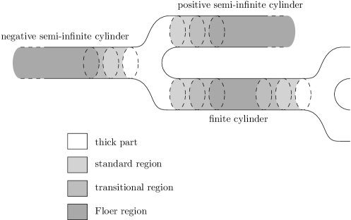
Figure 4.1. The decomposition of our surfaces. For simplicity, we have shown only part of the surface, omitting some of the positive semi-infinite cylinders.

The thick part is the rest of the surface, and can carry any one-form (4.1.16) (see Figure 4.1 for a summary).

Remark 4.1.9.

The conditions on the $\psi_{e}$ and on $\beta_{S}$ imply, via Stokes, that $\sigma_{0}>\sigma_{1}+\cdots+\sigma_{m}$.

We fix a Floer datum as in Section 4.1d, denoting it by $(H^{\mathrm{Floer}},J^{\mathrm{Floer}})$ for clarity. Concerning $(K_{S},J_{S})$ we make the following assumptions:

• over the thick part of the surface, as well the standard regions of the thin parts, we have $K_{S}={\textstyle\frac{1}{2}}\rho^{2}\beta_{S}$ on the cone of $\hat{N}$, and each $J_{S,z}$ is of contact type.

• Over the Floer region of the semi-infinite cylinders, we use the Floer Hamiltonian rescaled as in (4.1.37), $K_{S}=(H^{\mathrm{Floer}}_{t})^{(\sigma_{e})}\mathit{dt}$. For the almost complex structures, we allow any $J_{S,s,t}$ which are of contact type on $(iP/\sigma_{e})$-shells (for all $i\in{\mathbb{N}}$ such that $iP/\sigma_{e}>1$), and which as $s\rightarrow\pm\infty$ converge exponentially fast to $(J^{\mathrm{Floer}}_{t})^{(\sigma_{e})}$. This condition ensures good asymptotic behaviour of finite energy solutions of our Cauchy-Riemann equation, and is at the same time flexible enough for transversality purposes.

• There is more freedom on the Floer regions of the finite cylinders. We allow Hamiltonian terms of the form $K_{S}=H^{\mathrm{finite}}_{t}\mathit{dt}$, where on the cone $H^{\mathrm{finite}}_{t}=\frac{\sigma}{2}\rho^{2}+\tilde{H}^{\mathrm{finite}}_{t}$, for a perturbation $\tilde{H}^{\mathrm{finite}}$ which vanishes on $(iP/\sigma)$-shells. Moreover, on those shells, the almost complex structures should be of contact type. Of course, the $H^{\mathrm{finite}}$ do not have to be the same for two different finite cylinders.

• On the transition regions the Hamiltonian term should, on the cone of $\hat{N}$, satisfy

  (4.1.54) $$K_{S}={\textstyle\frac{1}{2}}\rho^{2}\psi(s)\mathit{dt}+\tilde{H}_{s,t}\mathit{dt},\;\text{ with }\;|\partial_{s}\tilde{H}_{s,t}|\leq-\psi^{\prime}(s)$$

  for some positive constant $c$, and where $\psi$ is the appropriate one of the functions (4.1.50), (4.1.52), (4.1.53). Moreover, $\tilde{H}_{s,t}$ should vanish on a sequence of shells, which is the same as for the (unique) adjacent Floer region. On those shells, we also require that the almost complex structures $J_{s,t}$ should be of contact type. To avoid confusion, let’s clarify that each transition region is treated separately here.

Lemma 4.1.10.

Over the Floer regions, the curvature $F_{S}$ is zero. Over the standard regions, the curvature is zero on the cone of $\hat{N}$. Over the transitional regions, the curvature is nonnegative (in fact positive) outside a compact subset of $\hat{N}$. Finally, over the thick part, the curvature is nonnegative on the cone.

Proof.

The only aspect which is not immediately obvious concerns the transitional regions. On such a region, (4.1.54) implies that on the cone of $\hat{N}$,

(4.1.55) $$F_{S}(\partial_{s},\partial_{t})=-\psi^{\prime}(s){\textstyle\frac{1}{2}}\rho^{2}+\partial_{s}\tilde{H}_{s,t}\geq-\psi^{\prime}(s)({\textstyle\frac{1}{2}}\rho^{2}-c).$$

That obviously makes the curvature positive where $\rho$ is large. ∎

Take one-periodic orbits $(x_{0},\dots,x_{m})$ of $(H_{t}^{\mathrm{Floer}})$. Consider solutions of the Cauchy-Riemann equation (4.1.6) whose asymptotics are appropriately rescaled version of these orbits:

(4.1.56) $$\textstyle\lim_{s\rightarrow\pm\infty}\lambda_{\hat{N},\log(\sigma_{e})}u(s,\cdot)=x_{e}\;\;\text{on the $e$-th semi-infinite cylinder.}$$

For such a solution, we have

(4.1.57) $$\frac{A(x_{0})}{\sigma_{0}}-\sum_{e=1}^{m}\frac{A(x_{e})}{\sigma_{e}}=E^{\mathrm{top}}(u)=E^{\mathrm{geom}}(u)+\int_{S}u^{*}F_{S}.$$

From Lemma 4.1.10, we see that there is a uniform lower bound on the curvature integral, that holds for any $u$. Hence, given $(x_{0},\dots,x_{m})$, there is an upper bound on the geometric energy, which is of course fundamental for compactness. The appropriate version of Proposition 4.1.7 is:

Proposition 4.1.11.

Fix one-periodic orbits $(x_{1},\dots,x_{m})$. Then, there is an $r$ such that every solution $u$ of the Cauchy-Riemann equation on $S$, with those limits over the positive semi-infinite cylinders, and arbitrary limit $x_{0}$ on the negative semi-infinite cylinder, is contained in $N_{r}$.

Proof.

From (4.1.57) we get a lower bound on $A(x_{0})$, given $(x_{1},\dots,x_{m})$. Hence, we may just as well work with a fixed $x_{0}$.

The first step is to bound the behaviour of $u$ on certain circles, one for each standard region. Take $C^{\mathrm{standard}}$ to be the closure of a standard region, identifying it with $[0,1]\times S^{1}$ by translation in $s$-direction. From (4.1.57) we get an a priori bound on $E^{\mathrm{geom}}(u|C^{\mathrm{standard}})\leq E^{\mathrm{geom}}(u)$. Let $T\subset S$ be the closure of the connected component of $S\setminus C^{\mathrm{standard}}$ which bounds $\{1\}\times S^{1}$; equivalently, this is the component not containing the negative semi-infinite cylinder. Let’s say that $T$ contains the $e$-th positive semi-infinite cylinders for $e\in E\subset\{1,\dots,m\}$. Then,

(4.1.58) $$A(u|\{1\}\times S^{1})=\sum_{e\in E}\frac{A(x_{e})}{\sigma_{e}}+E^{\mathrm{top}}(u|T)\geq\sum_{e\in E}\frac{A(x_{e})}{\sigma_{e}}+\int_{T}u^{*}F_{S}.$$

As before, there is an a priori lower bound for the curvature integral, and therefore for $A(u|\{1\}\times S^{1})$. Together, these bounds allow us to apply Lemma 4.1.3, and to obtain an $r\geq 1$ such that any solution $u$ must satisfy $u(s\times\{S^{1}\})\subset N_{r}$ for some $s\in[0,1]$. Since there are finitely many standard regions, we may choose $r$ so that the bound applies to all of them.

Let’s look at a connected component of the thick part. This is surrounded by standard regions, and in the closure of each standard region there is a circle that gets mapped to $N_{r}$. We can therefore enlarge our component by adding cylindrical pieces of those standard regions, and obtain a compact connected $C^{\mathrm{thick}}\subset S$ with nonempty boundary, such that $u(\partial C^{\mathrm{thick}})\subset N_{r}$. Notice that over $C^{\mathrm{thick}}$, we have $K_{S}={\textstyle\frac{1}{2}}\rho^{2}\beta_{S}$ on the cone, and all the almost complex structures are of contact type. We can therefore apply Lemma 4.1.4 to conclude that $u(C^{\mathrm{thick}})\subset N_{r}$.

Next, consider the negative semi-infinite cylinder. Since its piece $[-1,0]\times S^{1}$ is a standard region, we know that there is an $s\in[-1,0]$ such that $u(\{s\}\times S^{1})\subset N_{r}$. Moreover, $[s,0]\times S^{1}$ belonged to one of the previously considered regions $C^{\mathrm{thick}}$, so it remains to bound $u$ on $(-\infty,s]\times S^{1}$. From Lemma 4.1.10 we know that over this cylinder, $F_{S}$ is nonnegative outside $N_{\tilde{r}}$ for some $\tilde{r}$, which we can assume to be $\geq r$. We also know the limit $x_{0}$, hence may enlarge $\tilde{r}$ so that $x_{0}$ is contained in the interior of $N_{\tilde{r}}$. Finally, again making it larger, we can assume that $\tilde{r}$ is $P/\sigma_{0}$ times an integer. At this point, for any sufficiently negative $\tilde{s}$, we know that $u|[\tilde{s},s]\times S^{1}$ has the property that the boundary maps to $N_{\tilde{r}}$. One can apply Lemma 4.1.4 to conclude that the whole of $[\tilde{s},s]\times S^{1}$ gets mapped to $N_{\tilde{r}}$. For this, it is crucial that on the $\tilde{r}$-shell, the Hamiltonian is of standard form ${\textstyle\frac{1}{2}}\rho^{2}\beta$, and the almost complex structure of contact type; that is ensured by the choices we have made, including those for the transitional region $(-2,-1)\times S^{1}$.

The argument for the positive semi-infinite cylinders is parallel. That for the finite cylinders is also similar, but still deserves a short discussion. Such a cylinder $[-l,l]\times S^{1}$ has standard regions at its ends, so there are $s_{-}\in[-l,-l+1]$ and $s_{+}\in[l-1,l]$ such that $u(\{s_{\pm}\}\times S^{1})\subset N_{r}$. Moreover, as part of our discussion of the thick parts, we have already obtained a priori bounds on $u$ on $[-l,s_{-}]\times S^{1}$ and $[s_{+},l]\times S^{1}$. On the remaining part $[s_{-},s_{+}]\times S^{1}$, we will again apply the integrated maximum principle, bearing in mind that the $(iP/\sigma)$-shells can be used over that entire part. ∎

Proposition 4.1.12.

For a fixed choice of Floer datum $(H^{\mathit{Floer}},J^{\mathit{Floer}})$ and of one-form $\beta_{S}$, a generic choice of $(K_{S},J_{S})$ within the class above ensures that every solution to the Cauchy-Riemann equation is regular.

Sketch of proof.

Our main tool to achieve transversality is a generic choice of almost complex structures on the Floer regions of the semi-infinite cylinders. Of course, this freedom holds only away from the relevant shells, but because the limits are disjoint from those shells, so is $u(s,t)$ provided that $|s|\gg 0$.

One small wrinkle: there is a very restricted class of solutions whose transversality can’t be established in that way, namely ones which satisfy $\partial_{s}u=0$ for $|s|\gg 0$. Let’s look at such a $u$ on the negative semi-infinite cylinder (any other semi-infinite cylinder would also do). By unique continuation, we must have

(4.1.59) $$u(s,t)=\lambda_{\hat{N},-\log(\sigma_{0})}(x_{0}(t))\;\;\text{for all $s\leq-2$.}$$

In particular, on the Floer region, $u(s,t)$ is disjoint from the $(iP/\sigma_{0})$-shells. Hence, the same is true for $u(s,t)$ when $s$ is slightly larger than $-2$. But by looking at such $s$, we have reached into the transitional region, and the Hamiltonian term can then be chosen freely near $u(s,t)$ (subject to the bound (4.1.54), which is irrelevant since transversality is about infinitesimal considerations). Hence, one can use the freedom to change that Hamiltonian term to ensure that this special class of solutions is also regular. ∎

Finally, note that there is a rescaling process for data $(\beta_{S},J_{S},K_{S})$ as in (4.1.37): for $\tau\geq 1$, take

(4.1.60) $$\beta_{S}^{(\tau)}=\tau\beta_{S},$$

$$K_{S}^{(\tau)}=\lambda_{\hat{N},\log(\tau)}^{*}K_{S}/\tau,$$

$$J_{S}^{(\tau)}=\lambda_{\hat{N},\log(\tau)}^{*}J_{S}.$$

This still satisfies all the conditions imposed above, and the associated moduli spaces of maps can be identified with each other by taking $u^{(\tau)}=\lambda_{\hat{N},-\log(\tau)}u$.

4.1g. Parametrized moduli spaces

For many applications, one has to go beyond a single Riemann surface, and instead consider a manifold $\mathring{\mathfrak{P}}$ which parametrizes a family of punctured spheres, usually denoted by

(4.1.61) $$U_{\mathring{\mathfrak{P}}}\longrightarrow\mathring{\mathfrak{P}}.$$

This should carry a fibrewise one-form

(4.1.62) $$\beta_{\mathring{\mathfrak{P}}}\in\Omega^{1}(U_{\mathring{\mathfrak{P}}}/\mathring{\mathfrak{P}}),$$

satisfying the conditions from Section 4.1f on each fibre. There are a few notable points:

• the numbers $\sigma_{0},\dots,\sigma_{m}$ describing the behaviour of the one-form at infinity can vary throughout the family, which means that they are functions on $\mathring{\mathfrak{P}}$.

• The topological structure of the thick-thin decomposition is not necessarily constant throughout the family. Rather, it is sufficient that around each point of $\mathring{\mathfrak{P}}$, there should be a neighbourhood and a thick-thin decomposition with respect to which (4.1.62) satisfies the required properties. In practice, two thick-thin decompositions which may apply to the same point of $\mathring{\mathfrak{P}}$ only differ through forgetting some of the finite cylinders; we will say a little more about how these arise later on, when considering neck-stretching.

Similarly, we want to have a family version of the perturbation data from Section 4.1f,

(4.1.63) $$K_{\mathring{\mathfrak{P}}}\in\Omega^{1}(U_{\mathring{\mathfrak{P}}}/\mathring{\mathfrak{P}},\mathcal{H}(\hat{N}))\text{ and }J_{\mathring{\mathfrak{P}}}\in C^{\infty}(\mathcal{U}_{\mathring{\mathfrak{P}}},\mathcal{J}(\hat{N})),$$

Again, the devil lies in the details:

• The Floer datum involved is always the same (constant over $\mathring{\mathfrak{P}}$).

• As before, it is sufficient to have thick-thin decompositions locally on $\mathring{\mathfrak{P}}$. Again locally on $\mathring{\mathfrak{P}}$, one should be able to choose the constant $c$ which appears in (4.1.54) independently of the parameters.

• For the behaviour of the almost complex structures on the Floer regions of the semi-infinite cylinders, the $C^{\infty}$ condition as formulated in (4.1.63) is not enough. Instead, in a local trivialization of our family (around some point of $\mathring{\mathfrak{P}}$) where $r$ are the parameters, we must have that $J_{\mathring{\mathfrak{P}},r,s,t}\rightarrow(J_{t}^{\mathrm{Floer}})^{(\sigma_{e})}$ exponentially as $s\rightarrow\pm\infty$, and uniformly in $r$. This means that in any $C^{k}$ norm (derivatives with respect to $r,s,t$), the difference between the two is bounded by $Ae^{\mp Bs}$, where $A,B>0$ are independent of $r$. (In addition, one of course has restrictions on the behaviour on shells.)

Given a collection of orbits $\mathbf{x}=(x_{0},x_{1},\cdots,x_{m})$, let $\mathring{\mathfrak{P}}(\mathbf{x})$ denote the moduli space of pairs

(4.1.64) $$p\in\mathring{\mathfrak{P}},\;u:S=U_{p}\longrightarrow\hat{N},$$

where $U_{p}$ is the fibre of (4.1.61), and $u$ is a solution of (4.1.6) with asymptotics (4.1.56). There is an straightforward parametrized version of Proposition 4.1.12, saying that this space is regular for generic choice of (4.1.63).

The analogue of (4.1.46) is a canonical isomorphism

(4.1.65) $$\lambda^{\mathrm{top}}T_{(p,u)}\mathring{\mathfrak{P}}(\mathbf{x})\cong T_{p}\mathring{\mathfrak{P}}\otimes\mathit{det}(D_{u}).$$

Here, $D_{u}$ is the ordinary linearized operation, which comes with versions of (4.1.43) and (4.1.44):

(4.1.66) $$\mathrm{index}(D_{u})=\mathrm{deg}(x_{0})-\mathrm{deg}(x_{1})-\cdots-\mathrm{deg}(x_{m}),$$

(4.1.67) $$\mathit{det}(D_{u})\otimes\mathfrak{o}_{x_{1}}\otimes\cdots\otimes\mathfrak{o}_{x_{m}}\cong\mathfrak{o}_{x_{0}}.$$

The combination of this and (4.1.65) yields

(4.1.68) $$\mathrm{dim}\,\mathring{\mathfrak{P}}(\mathbf{x})=\mathrm{dim}\,\mathring{\mathfrak{P}}+\mathrm{deg}(x_{0})-\mathrm{deg}(x_{1})-\cdots-\mathrm{deg}(x_{m}),$$

(4.1.69) $$o(p,u):\lambda^{\mathrm{top}}(T_{(p,u)}\mathring{\mathfrak{P}}(\mathbf{x}))\otimes\mathfrak{o}_{x_{1}}\otimes\cdots\otimes\mathfrak{o}_{x_{m}}\cong\lambda^{\mathrm{top}}(T_{p}\mathring{\mathfrak{P}})\otimes\mathfrak{o}_{x_{0}}.$$

Let’s assume that an orientation of $\mathring{\mathfrak{P}}$ has been chosen, and that $(p,u)$ is an isolated point in the parameterized moduli space. In that case, (4.1.69) simplifies to an isomorphism $\mathfrak{o}_{x_{1}}\otimes\cdots\otimes\mathfrak{o}_{x_{m}}\cong\mathfrak{o}_{x_{0}}$. In principle, the ${\mathbb{K}}$-normalization of this isomorphism describes the contribution of $(p,u)$ to a map

(4.1.70) $$\mathit{CF}^{*}(H^{\mathrm{Floer}})^{\otimes m}\longrightarrow\mathit{CF}^{*}(H^{\mathrm{Floer}})[-\mathrm{dim}(\mathring{\mathfrak{P}})].$$

As just described, the construction would only work for compact $\mathring{\mathfrak{P}}$, which rarely applies. Instead, one usually encounters compactifications of the parameter space obtained by allowing the surfaces to split into pieces via neck-stretching, and that will be the next topic in our exposition.

4.1h. Neck-stretching

Let’s consider a simple situation, where we have surfaces $S_{-}$ and $S_{+}$, each of them coming with all the structure introduced above: one-forms $\beta_{S_{\pm}}$, and numbers $(\sigma_{\pm,e})$ which describe those one-forms on the Floer regions of the semi-infinite cylinders. Let $\varepsilon_{-}:(-\infty,0]\times S^{1}\rightarrow S_{-}$ be the unique negative end, and $\varepsilon_{+}:[0,\infty)\times S^{1}\rightarrow S_{+}$ one of the positive ends. The glued surface, for some length $l>2$, is

(4.1.71) $$S_{l}\stackrel{{\scriptstyle\mathrm{def}}}{{=}}\frac{(S_{+}\setminus\varepsilon_{+}((l,\infty)\times S^{1}))\sqcup(S_{-}\setminus\varepsilon_{-}((-\infty,-l)\times S^{1}))}{\varepsilon_{+}(s,t)\sim\varepsilon_{-}(s-l,t)}.$$

To make the one-forms compatible, we multiply them by some constants

(4.1.72) $$\tau_{\pm}\geq 1,\;\;\text{ such that }\tau_{-}\sigma_{-,e}=\tau_{+}\sigma_{+,0}.$$

Then, $S_{l}$ will come with one-forms $\beta_{S_{l}}$. Gluing creates a finite cylinder $[0,l]\times S^{1}\subset S_{l}$. For large values $l\gg 0$, we consider $S_{l}$ as having the thick-thin decomposition inherited from $S_{\pm}$ including that cylinder. However, as $l$ becomes smaller, we will forget that cylinder, which means that it will belong to the thick part of $S_{l}$ (this is the previously mentioned phenomenon that the thick-thin decomposition can be parameter-dependent).

Instead of the gluing length, we also often use a gluing parameter $\gamma\in\mathring{\mathfrak{P}}=(0,e^{-2})$, with the relation between the two given by

(4.1.73) $$l=-\log(\gamma).$$

One can think of the glued surfaces as fibres of a family of Riemann surfaces parametrized by $\gamma$. That family can then be extended over $\gamma=0$ by setting the fibre there to be $S_{-}\sqcup S_{+}$. The outcome is a three-manifold $U_{\mathfrak{P}}$ with boundary, with a local submersion

(4.1.74) $$U_{\mathfrak{P}}\longrightarrow\mathfrak{P},$$

where $\mathfrak{P}=[0,e^{-2})$. The one-forms we have constructed, and the original $\beta_{S_{\pm}}$, then yield a smooth fibrewise one-form

(4.1.75) $$\beta_{\mathfrak{P}}\in\Omega^{1}(U_{\mathfrak{P}}/\mathfrak{P}).$$

Suppose that $S_{\pm}$ come with perturbation data. Concerning the data on the glued family, these should smoothly extend to $\gamma=0$, which means we have

(4.1.76) $$K_{\mathfrak{P}}\in\Omega^{1}(U_{\mathfrak{P}}/\mathfrak{P},\mathcal{H}(\hat{N}))\text{ and }J_{\mathfrak{P}}\in C^{\infty}(U_{\mathfrak{P}},\mathcal{J}(\hat{N})),$$

which on the fibre $S_{+}\sqcup S_{-}$ reduce to versions of $(K_{S_{\pm}},J_{S_{\pm}})$ rescaled by $\tau_{\pm}$ in the sense of (4.1.60). Fibrewise, this should satisfy our usual conditions, but some additional restrictions have to be imposed as well.

• The constant $c$ appearing in (4.1.54) can be chosen the same for all $S_{l}$, $l\gg 0$, as well as for $S_{\pm}$.

• On the semi-infinite ends of the glued surfaces, one needs to have exponential converge to $(J_{t}^{\mathit{Floer}})^{(\sigma_{e})}$ uniformly in the gluing parameter $\gamma$.

• On the finite cylinder $[0,l]\times S^{1}$ obtained from gluing, the difference between the almost complex structure on the glued surface and the appropriate $(J_{t}^{\mathit{Floer}})^{(\sigma)}$ must be bounded by $A(e^{-Bs}+e^{B(s-l)})$, where $A,B>0$ are constants independent of the gluing length.

The aim of these requirements is to ensure suitable compactness properties in the parametrized moduli space. These are based on the following:

Proposition 4.1.13.

Energy bounds on solutions $u:S_{l}\rightarrow\hat{N}$ of the Cauchy-Riemann equation, as well as the key a priori bound (Proposition 4.1.11), apply uniformly as $l\rightarrow\infty$.

Sketch of proof.

What’s important here is that the curvature integral appearing in (4.1.57) will have an a priori lower bound that holds for all $l$, because the variable-length part $[-l+2,l-2]\times S^{1}$ contributes zero. For the constant appearing in (4.1.54), we have explicitly asked that an $l$-independent bound should hold. The outcome is that the bound on the geometric energy, and Proposition 4.1.11, apply uniformly over all $S_{l}$. ∎

The discussion above is a model for what happens near codimension-one faces of general parameter spaces $\mathfrak{P}$. Our spaces $\mathfrak{P}$ will be manifolds with corners, where the strata of codimension $k$ correspond to splittings of the surfaces into $k$ pieces. They carry extended universal families which generalize that in (4.1.74), and which come with thick-thin decompositions (and in particular ends) compatible with gluing. We then choose perturbation data over the compactified parameter space generalizing (4.1.76) which near each codimension $k$ face satisfies the above conditions with respect to the gluing parameters $\gamma_{1},\cdots,\gamma_{k}$ near that stratum. We summarize this by saying that $(K_{\mathfrak{P}},J_{\mathfrak{P}})$ is conformally consistent.

4.2. The Lagrangian (and mixed) theory

4.2a. Geometric setup

We again begin with a review of generalities. Suppose $(N,\theta_{N})$ is a Liouville domain and $(\hat{N},\theta_{\hat{N}})$ is its symplectic completion (see Section 4.1b). Let $S$ be an oriented surface with boundary, which comes with a Hamiltonian term (4.1.1). In addition, we want our surface to be equipped with an exact Lagrangian boundary condition, meaning a submanifold and function

(4.2.1) $$L_{\partial S}\subset\partial S\times\hat{N},$$

$$G_{\partial_{S}}:L_{\partial S}\longrightarrow{\mathbb{R}},$$

such that $L_{\partial S}\rightarrow\partial S$ is a fibre bundle, and $dG_{\partial S}|L_{\partial S,z}=\theta_{\hat{N}}|L_{\partial S,z}\in\Omega^{1}(L_{\partial S,z})$ for each $z\in\partial S$. The boundary curvature $F_{\partial S}$ is a one-form on $L_{\partial S}$ which vanishes when restricted to a fibre, given by

(4.2.2) $$F_{\partial S}=dG_{\partial S}-\theta_{\hat{N}}|L_{\partial S}+K_{S}|L_{\partial S}.$$

Thinking of the connection given by $K_{S}$, one can explain the geometric meaning of (4.2.2) as follows: $L_{\partial S}$ is compatible with parallel transport along $\partial S$ if and only if $(\omega_{\hat{N}}-dK_{S})|L_{\partial S}=0$, which is the case iff $F_{\partial S}$ is locally the pullback of a one-form on $\partial S$. (Actual vanishing of $F_{\partial S}$ lifts that compatibility statement from Hamiltonian vector fields to the level of functions.)

Take a map $u:S\rightarrow\hat{N}$, satisfying

(4.2.3) $$u(z)\in L_{\partial S,z}\;\;\text{ for all $z\in\partial S$.}$$

Given a path $c:[0,1]\rightarrow S$ with $c(0),c(1)\in\partial S$, the action of $u$ along $c$ is defined as

(4.2.4) $$A(u|c)=\Big{(}\int_{c}-u^{*}\theta_{\hat{N}}+u^{*}K_{S}\Big{)}+G_{\partial S}(c(1),u(c(1)))-G_{\partial S}(c(0),u(c(0))).$$

One can add up that term for several paths, and also allow loops as in (4.1.4), to get a definition of action for relative one-cycles in $(S,\partial S)$. Let $C\subset S$ be a compact subdomain, whose boundary consists of $\partial^{\mathrm{para}}C=C\cap\partial S$ and additional intervals and circles $\partial^{\mathrm{trans}}C$; the two parts are required to meet transversally, so $C$ is a surface with corners. The topological energy of $u$ on $C$ is

(4.2.5) $$E^{\mathrm{top}}(u|C)=\int_{C}u^{*}\omega_{\hat{N}}-d(u^{*}K_{S})+\int_{\partial^{\mathrm{para}}C}u^{*}F_{\partial S}=-A(u|\partial^{\mathrm{trans}}C).$$

For solutions of the Cauchy-Riemann equation (4.1.6) satisfying (4.2.3), we now have

(4.2.6) $$E^{\mathrm{geom}}(u|C)=E^{\mathrm{top}}(u|C)-\int_{C}u^{*}F_{S}-\int_{\partial^{\mathrm{para}}C}u^{*}F_{\partial S}.$$

In our application, we will only use exact Lagrangian submanifolds $L$ which are of Legendrian type on the cone, which means

(4.2.7) $$L\cap([1,\infty)\times\partial N)=[1,\infty)\times\Lambda$$

for some Legendrian $\Lambda\subset\partial N$. Each $L$ should come with a primitive $\theta_{\hat{N}}|L=dG_{L}$ which vanishes on (4.2.7). When dealing with surfaces $S$, we want the one-forms (4.1.16) to also satisfy

(4.2.8) $$\beta_{S}|\partial S=0\in\Omega^{1}(\partial S).$$

For the associated Lagrangian boundary conditions, we require that the part of $L_{\partial S}$ lying in the cone of $\hat{N}$ is locally constant in $z$, and that $G_{\partial S}$ vanishes on the cone. If we then suppose that $K_{S}={\textstyle\frac{1}{2}}\rho^{2}\beta_{S}$ on the cone, it follows that the boundary curvature (4.2.2) is zero there.

4.2b. A priori bounds

We consider solutions of (4.1.6) with boundary conditions (4.2.3). The analogue of Lemma 4.1.3 is:

Lemma 4.2.1.

Take a rectangular region $C=[0,1]^{2}\subset S$ (with $\partial^{\mathrm{para}}C=[0,1]\times\{0,1\}$ and $\partial^{\mathrm{trans}}C=\{0,1\}\times[0,1]$). Suppose that on this region, the same conditions on $(J_{S},K_{S})$ as in Lemma 4.1.3 apply, and so does (4.1.17). Then, with (4.1.18) replaced by its obvious analogue

(4.2.9) $$A(u|\{1\}\times[0,1])\geq a,$$

the same conclusion holds, where the constant $r$ additionally depends on $G_{\partial S}$.

Proof.

One has (4.1.20) as before. The analogue of (4.1.21) says that if $u(\{s\}\times[0,1])$ lies in the cone,

(4.2.10) $$A(u|\{s\}\times[0,1])\leq\frac{1}{\sigma}\int_{\{s\}\times[0,1]}\|\partial_{t}u-Y_{S}(\partial_{t})\|^{2}-\frac{\sigma}{4}\int_{s\times[0,1]}\rho^{2}(u).$$

In addition to the bound (4.1.22) on the curvature, we also have

(4.2.11) $$|F_{\partial S}|\leq c.$$

The analogue of (4.1.23) is

(4.2.12) $$A(u|\{s\}\times[0,1])\geq a-b-2c.$$

From the energy bound, there must be some $s\in[0,1]$ such that

(4.2.13) $$\int_{\{s\}\times[0,1]}\|\partial_{t}u-Y_{S}(\partial_{t})\|^{2}\leq e.$$

For that value of $s$, we have (4.1.25) as well as

(4.2.14) $$\int_{\{s\}\times[0,1]}\rho^{2}(u)\leq\frac{4}{\sigma}(b+2c-a)+\frac{4}{\sigma^{2}}e\quad\text{ if $u(\{s\}\times[0,1])$ lies in the cone.}$$

One concludes the argument as before. ∎

The original version of the integrated maximum principle [4, Lemma 7.2] already allows for Lagrangian boundary conditions. We reproduce it here for ready citeability. The proof is the same as in Lemma 4.1.4 (with $\partial D$ replaced by $\partial^{\mathrm{trans}}D$).

Lemma 4.2.2.

Let $C\subset S$ be a connected compact subdomain, such that $\partial^{\mathit{trans}}C\neq\emptyset$. For some $r\geq 1$, suppose that the assumptions from Lemma 4.1.4 on $(K_{S},J_{S},F_{S})$ hold. Let $u:S\rightarrow\hat{N}$ be a solution of (4.1.6), (4.2.3), such that $u(\partial^{\mathrm{trans}}C)\subset N_{r}$. Then $u(C)\subset N_{r}$.

4.2c. Floer cohomology

Fix a pair of Lagrangian submanifolds $L_{k}$ ($k=0,1$), as well as some $P>1$. The following assumption will allow us to use Hamiltonians which are (unperturbed) quadratic on the cone.

Assumption 4.2.3.

For the associated Legendrian submanifolds $(\Lambda_{0},\Lambda_{1})$, all Reeb chords of length $\geq 1$ are nondegenerate. Moreover, there are no Reeb chords whose length is a positive integer multiple of $P$.

A Floer datum is given by $H=(H_{t})_{t\in[0,1]}$ and $J=(J_{t})_{t\in[0,1]}$, such that:

• on the cone, $H_{t}={\textstyle\frac{1}{2}}\rho^{2}$. As a consequence, Floer chords which intersect the cone must lie entirely inside it, and can be identified with Reeb chords of length $\rho\geq 1$; these are nondegenerate by assumption. We then also require all other chords to be nondegenerate.

• For each $i\in{\mathbb{N}}$, there is an $iP$-shell on which $J$ is contact type. These shells must be disjoint from the Floer chords.

The counterpart of Lemma 4.1.6 is trivially satisfied, since the Floer chords that correspond to length $\rho$ Reeb chords have action $-{\textstyle\frac{1}{2}}\rho^{2}$. For solutions $u:{\mathbb{R}}\times[0,1]\rightarrow\hat{N}$ of Floer’s equation with boundary conditions $(L_{0},L_{1})$, we have the analogue of Lemma 4.1.7, using Lemma 4.2.2 in the same way as before:

Lemma 4.2.4.

Fix a Floer chord $y_{1}$. There is an $r$ such that any Floer solution with positive limit $y_{1}$, and arbitrary negative limit $y_{0}$, is contained in $N_{r}$.

The rescaling trick (4.1.37) now additionally involves moving the Lagrangian submanifolds (and the corresponding primitives)

(4.2.15) $$L^{(\sigma)}=\lambda_{\hat{N},-\log(\sigma)}(L),$$

$$G^{(\sigma)}=\lambda_{\hat{N},\log(\sigma)}^{*}G_{L}/\sigma.$$

This pushes $L$ inwards, so we still have $L^{(\sigma)}=[1,\infty)\times\Lambda$ on the cone. One gets a canonical isomorphism between the Floer complex for $(L_{0},L_{1},H,J)$ and $(L_{0}^{(\sigma)},L_{1}^{(\sigma)},H^{(\sigma)},J^{(\sigma)})$.

Again, because the almost complex structure is unconstrained near the Floer chords, a generic choice of that structure achieves regularity of the moduli spaces. To define the Floer complex with a ${\mathbb{Z}}$-grading and ${\mathbb{K}}$-coefficients, we assume the following standard “brane conditions”:

(4.2.16) our Lagrangian submanifolds carry gradings with respect to the trivialization of the line bundle from (4.1.38) (and hence come with orientations). Additionally they are equipped with Spin structures.

Then, as in the closed-string case, each chord $y$ has an associated degree $\mathrm{deg}(y)$ and determinant line $\mathfrak{o}_{y}=\operatorname{det}(D_{y})$. In parallel with (4.1.42) one sets

(4.2.17) $$\mathit{CF}^{k}(L_{0},L_{1},H)=\bigoplus_{\mathrm{deg}(y)=k}|\mathfrak{o}_{y}|_{\mathbb{K}}.$$

Given two chords, $\mathring{\mathfrak{R}}(y_{0},y_{1})$ denotes the moduli space of Floer strips up to ${\mathbb{R}}$-translation. Assuming regularity, any $u$ in that space determines an isomorphism $o(u)$ as in (4.1.47), which for isolated strips reduces to an isomorphism $\mathfrak{o}_{y_{1}}\cong\mathfrak{o}_{y_{0}}$. One again defines the Floer differential by adding up the ${\mathbb{K}}$-normalizations of those isomorphisms.

4.2d. Open string operations

Let $(S,j_{S})$ be a boundary-punctured disc, obtained by removing $n+1>0$ boundary points from a closed disc; we label those missing boundary points by $\{0,\dots,n\}$, going counterclockwise around the boundary. We correspondingly label the connected components of $\partial S$, so that the $0$-th boundary component joins the $0$-th and $1$-st boundary puncture. Our surface should come with a one-form satisfying (4.1.16) and (4.2.8). As before, we want a decomposition of $S$ into thick and thin pieces, and of the latter pieces into three types of regions (see Figure 4.2; note though that the “transitional” regions play a much smaller role than before, and exist only for a very technical transversality reason). The thin pieces are:

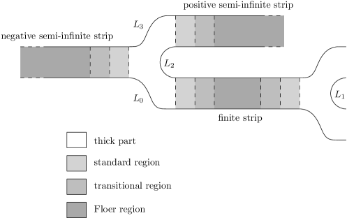
Figure 4.2. The decomposition of surfaces in the open string case.

• A single negative semi-infinite strip $(-\infty,0]\times[0,1]\hookrightarrow S$ asymptotic to the $0$-th boundary puncture (here and in similar situations below, it is understood that $(-\infty,0]\times\{0,1\}$ is mapped to $\partial S$). This comes with a constant $\sigma_{0}$ and function $\psi_{0}$ as in (4.1.50), with $\beta_{S}=\psi_{0}(s)\mathit{dt}$. The Floer region is $(-\infty,-2]\times[0,1]$; the transitional one, $(-2,-1)\times[0,1]$; and the standard region, $[-1,0]\times[0,1]$.

• Positive semi-infinite strips $[0,\infty)\times[0,1]\rightarrow S$ for the boundary punctures labeled $e\in\{1,\dots,n\}$, with constants $\sigma_{e}\geq 1$, functions $\psi_{e}$ as in (4.1.52), and $\beta_{S}=\psi_{e}(s)\mathit{dt}$. The Floer regions are $[2,\infty)\times[0,1]$; the transitional ones, $(1,2)\times[0,1]$; and the standard regions, $[0,1]\times[0,1]$.

• Some number (which can be zero) of finite strips, $[-l,l]\times[0,1]\hookrightarrow 0$ for $l>2$. The parametrization is always such that $\{-l\}\times[0,1]$ borders the component of $S\setminus((-l,l)\times[0,1])$ which contains the negative semi-infinite strip. Each finite strip comes with its own constant $\sigma$ and function $\psi$ as in (4.1.53), with $\beta_{S}=\psi(s)\mathit{dt}$. The Floer region of such a strip is $[-l+2,l-2]\times[0,1]$; the transitional regions are $(-l+1,-l+2)\times[0,1]$ and $(l-2,l-1)\times[0,1]$; and the standard regions, $[-l,-l+1]\times[0,1]$ and $[l-1,1]\times[0,1]$.

Fix Lagrangian submanifolds $(L_{0},\dots,L_{n})$. Choose Floer data $(H^{\mathrm{Floer}}_{e},J^{\mathrm{Floer}}_{e})$, $e\in\{0,\dots,n\}$, associated to the pairs $(L_{0},L_{n})$ (for $e=0$) and $(L_{e-1},L_{e})$ (for $e=1,\dots,n$). Each such pair is required to satisfy Assumption 4.2.3 (with the same constant $P$). Our surface will come with a Lagrangian boundary condition $(L_{\partial S},G_{\partial S})$, as well as the usual $(K_{S},J_{S})$. Concerning those, we make the following assumptions:

• Everywhere on the surface, we have that $K_{S}={\textstyle\frac{1}{2}}\rho^{2}\beta_{S}$ on the cone of $\hat{N}$. Similarly, everywhere on the $i$-th boundary component of $S$, we have $L_{\partial S}=L_{i}$ on the cone.

• Over the thick part of $S$, as well as the standard regions, $J_{S}$ is of contact type.

• Take the Floer region of the $e$-th semi-infinite strip (for any $e$). On that region, the Lagrangian boundary condition is

  (4.2.18) $$\left.\begin{aligned} &L_{\partial S,0,t}=L_{0}^{(\sigma_{0})}\\ &L_{\partial S,1,t}=L_{n}^{(\sigma_{0})}\end{aligned}\right\}\text{ if $e=0$, or }\quad\left.\begin{aligned} &L_{\partial S,0,t}=L_{e-1}^{(\sigma_{0})}\\ &L_{\partial S,1,t}=L_{e}^{(\sigma_{0})}\end{aligned}\right\}\text{ if $e>0$,}$$

  with corresponding functions as in (4.2.15). The Hamiltonian term is $K_{S}=(H^{\mathrm{Floer}}_{e,t})^{(\sigma_{e})}\mathit{dt}$. The almost complex structure $J_{S,s,t}$ is of contact type on $(iP/\sigma_{e})$-shells and as $s\rightarrow\pm\infty$, converges exponentially to $(J^{\mathrm{Floer}}_{e,t})^{(\sigma_{e})}$.

• On the Floer region of any finite strip, we want $K_{S}=H^{\mathrm{finite}}_{t}\mathit{dt}$, where $H^{\mathrm{finite}}_{t}=\frac{\sigma}{2}\rho^{2}$ on the cone. Similarly, the Lagrangian boundary condition and function $G_{\partial S}$ should be independent of $s$. Finally, the almost complex structures should be of contact type on $(iP/\sigma)$-shells.

• On any transitional region, we want the almost complex structures to be of contact type for the same shells as the (unique) adjacent Floer region.

We consider solutions of (4.1.6), (4.2.3) with asymptotics which are rescaled Lagrangian chords,

(4.2.19) $$\textstyle\lim_{s\rightarrow\pm\infty}\lambda_{\hat{N},\log(\sigma_{e})}u(s,\cdot)=x_{e}.$$

The analogue of (4.1.57) is

(4.2.20) $$\frac{A(x_{0})}{\sigma_{0}}-\sum_{e=1}^{n}\frac{A(x_{e})}{\sigma_{e}}=E^{\mathrm{top}}(u)=E^{\mathrm{geom}}(u)+\int_{S}u^{*}F_{S}+\int_{\partial S}u^{*}F_{\partial S}.$$

As before, we have a uniform lower bound on the two curvature terms (in fact, the $\partial S$ term is bounded both below and above). The following is the counterpart of Proposition 4.1.11; the proof remains the same, with the basic analytic ingredients are replaced by their open string counterparts (Lemma 4.2.1 and 4.2.2).

Proposition 4.2.5.

Fix Floer chords $(y_{1},\dots,y_{m})$. Then, there is an $r$ such that every solution $u$ of the Cauchy-Riemann equation on $S$, with those limits over the positive semi-infinite strips, and arbitrary limit $y_{0}$ on the negative semi-infinite strip, is contained in $N_{r}$.

We also have a transversality result, analogous to Proposition 4.1.12. As in that situation, there is an unlikely exceptional case which has to be considered separately. Namely, suppose we have a solution which, on the negative semi-infinite strip, is of the form (4.1.59). There are two sub-cases to consider:

• The rescaled orbit $\lambda_{\hat{N},-\log(\sigma_{0})}(y_{0}(t))$ is disjoint from the cone of $\hat{N}$. In that case, at a point $u(s,t)$ with $s$ slightly larger than $-2$, one can choose $K_{S}$ freely, and transversality can be established by varying it there, just as in the closed string case.

• The rescaled orbit $\lambda_{\hat{N},-\log(\sigma_{0})}(y_{0}(t))$ lies in the cone of $\hat{N}$. Suppose temporarily that there is some $s_{*}\in(-2,-1)$ such that on the region $[-2,s_{*}]\times[0,1]$, we have $\partial_{s}u=0$. This also means that $\partial_{t}u=\psi(s)\rho R$, where $\rho\geq 1$ is constant; but those two conditions contradict each other, because $\psi^{\prime}(s)<0$. As a consequence, we see that there points $(s,t)\in(-2,-1)\times[0,1]$ with $s$ arbitrarily close to $-2$, where $\partial_{s}u$ is nonzero. At such a point, $u(s,t)$ will be disjoint from $(iP/\sigma)$-shells, hence the almost complex structure can be varied freely, which ensures transversality.

The discussion of parametrized moduli spaces is parallel to that in Section 4.1e, and there is a notion of conformally consistent perturbations parallel to that from Section 4.1h. We will not go through the details.

4.2e. Closed-open and open-closed situations

Finally, we will encounter setups that mix the open and closed string theory, of two different kinds. In the first situation (closed-open) we consider Riemann surfaces obtained from the closed disc by removing $m$ interior points, labeled as $\{1,\dots,m\}$ and $(d+1)$ boundary points, labeled as $\{0,\dots,d\}$. The $0$-th boundary point corresponds to a negative semi-infinite strip, and the others have positive (cylindrical or strip) ends. In the second situation (open-closed), we have $(m+1)$ interior points, one of which is negative, and $n$ positive boundary punctures.

In this context, the thick pieces can be more general than before, since they can both include parts of $\partial S$ and have boundary circles. However, that does not matter: we continue to impose the same conditions on $(K_{S},J_{S})$ on such pieces, which were the same in our discussion of closed and open string operations. All other pieces (finite and semi-infinite cylinders, finite and semi-infinity strips) belong to the one of the two setups encountered before, and we adopt our previous treatment of them.

5. Deformed symplectic cohomology

This section sets up certain specific operations in Hamiltonian Floer cohomology. For the analysis, we use the framework from Section 4.1 without further elaboration. We apply that framework to a number of specific families of punctured Riemann surfaces, and the bulk of the discussion will be taken up with defining those. Concretely, we start with the $L_{\infty}$-algebra structure on the chain complex underlying symplectic cohomology; this serves as prototype and will therefore be worked out in more detail. There is a related $L_{\infty}$-module structure, which admits a lift to $S^{1}$-equivariant Floer cohomology. (One could see all of this as consequences of having the structure of an algebra over the chain level framed Deligne-Mumford operad, but implementing that larger structure Floer-theoretically requires considerable effort [3]; hence, we follow the conventional strategy of just using geometrically defined chains which are specifically tailored to the operations under discussion.)

Following those general constructions, we assume that a Maurer-Cartan element in the $L_{\infty}$-algebra is given (with a formal variable $q$). This element gives rise to formal deformations of all Floer cohomology groups involved. Finally, and most importantly for our application, we define the connection $\nabla_{u\partial_{q}}$ on deformed $S^{1}$-equivariant symplectic cohomology.

5.1. Deligne-Mumford spaces and their relatives

5.1a. Deligne-Mumford spaces

Consider spheres (4.1.48) with $m+1\geq 3$ punctures. We assume $z_{0}=\infty$ and write

(5.1.1) $$S={\mathbb{C}}\setminus\{z_{1},\dots,z_{m}\}.$$

The parameter space is

(5.1.2) $$\mathring{\mathfrak{M}}_{m}=\mathit{Conf}_{m}({\mathbb{C}})/({\mathbb{C}}\rtimes{\mathbb{C}}^{*}),$$

where $\mathit{Conf}$ is ordered configuration space. Strata of the Deligne-Mumford compactification $\mathfrak{M}_{m}$ are labeled by trees, for which we use the following terminology.

• A tree $T$ is a contractible graph with directed edges, such that every vertex has exactly one outgoing edge. We write $|v|_{\operatorname{in}}=|v|-1$ for the number of incoming edges.

• Our trees have $(m+1)$ semi-infinite edges, of which $1$ is directed towards infinity (outgoing), and $m$ are directed away from infinity (incoming). There is a unique vertex (the root vertex $v_{\operatorname{root}}$) adjacent to the outgoing edge.

• As part of the data of a tree, we fix a labeling of the incoming semi-infinite edges as $\{1,\dots,m\}$ (if two trees are isomorphic, the isomorphism between them is unique, since it has to preserve the labels). The outgoing edge can then be labeled as $0$.

Given that,

(5.1.3) $$\mathfrak{M}_{m}=\bigsqcup_{T}\mathring{\mathfrak{M}}_{T},\quad\mathring{\mathfrak{M}}_{T}=\prod_{v}\mathring{\mathfrak{M}}_{|v|_{\operatorname{in}}},$$

where the union is over all stable trees $T$, meaning trees such that each vertex has $\geq 2$ incoming edges. (More precisely, we pick a representative in each isomorphism class of trees; the resulting $\mathring{\mathfrak{M}}_{T}$ is independent of that choice up to canonical isomorphism.) The tree with only one vertex corresponds to the inclusion $\mathring{\mathfrak{M}}_{m}\subset\mathfrak{M}_{m}$. The space $\mathfrak{M}_{m}$ has a natural structure of a compact complex manifold, and the stratification in (5.1.3) is given by a normal crossing divisor inside that manifold. Each point of $\mathfrak{M}_{m}$ corresponds to a disconnected Riemann surface $S=\bigsqcup_{v}S_{v}$, with components as in (5.1.1).

5.1b. The framed version

A framing at $z_{k}\in\bar{S}={\mathbb{C}}P^{1}$ is a distinguished tangent direction

(5.1.4) $$\tau_{z_{k}}\in(T_{z}\bar{S}\setminus\{0\})/{\mathbb{R}}^{>0}\cong S^{1}.$$

Since we work primarily with the punctured surface $S$ obtained by removing the $z_{k}$, the framings may be more appropriately called by their Floer-theoretic name, asymptotic markers. Punctured spheres with asymptotic markers (at all $z_{k}$) are parametrized by a space $\mathring{\mathfrak{M}}_{m}^{\operatorname{fr}}$, which is an $(S^{1})^{m+1}$-bundle over $\mathring{\mathfrak{M}}_{m}$. It has a compactification to a smooth manifold with corners $\mathfrak{M}_{m}^{\operatorname{fr}}$, whose strata are analogous to (5.1.3):

(5.1.5) $$\mathfrak{M}_{m}^{\operatorname{fr}}=\bigsqcup_{T}\mathring{\mathfrak{M}}_{T}^{\operatorname{fr}},\quad\mathring{\mathfrak{M}}_{T}^{\operatorname{fr}}=\big{(}\prod_{v}\mathring{\mathfrak{M}}^{\operatorname{fr}}_{|v|_{\operatorname{in}}}\big{)}/(S^{1})^{E_{\mathit{fin}}(T)}.$$

Here, $E_{\mathit{fin}}(T)$ is the set of finite edges of $T$. Each such edge singles out two punctures, lying on different $S_{v}$, and the $S^{1}$-action rotates their markers in opposite directions. More geometrically, if we consider the compact connected nodal surface $\bar{S}=\bigcup_{v}\bar{S}_{v}$ corresponding to a point of $\mathfrak{M}_{m}^{\operatorname{fr}}$, this comes equipped with framings at the $z_{k}$, as well as relative framings at all nodes $z=\bar{S}_{v_{1}}\cap\bar{S}_{v_{2}}$, meaning distinguished elements

(5.1.6) $$\tau_{z}^{\mathit{rel}}\in\big{(}(T_{z}\bar{S}_{v_{1}}\otimes T_{z}\bar{S}_{v_{2}})\setminus\{0\}\big{)}/{\mathbb{R}}^{>0}\cong S^{1}.$$

Remark 5.1.1.

The space $\mathfrak{M}_{m}^{\operatorname{fr}}$ was constructed in [51]. As an intermediate object, they first introduced another space $\mathfrak{M}_{m}^{\mathit{bl}}$, obtained by taking a real oriented blowup of all the strata in Deligne-Mumford space. Since the stratification has normal crossings, blowing up yields a smooth (in fact real-analytic) manifold with corners. Geometrically, this corresponds to adding relative framings (5.1.6) only. One then has a principal bundle

(5.1.7) $$(S^{1})^{m+1}\longrightarrow\mathfrak{M}_{m}^{\operatorname{fr}}\longrightarrow\mathfrak{M}_{m}^{\mathit{bl}}.$$

5.1c. The symmetric group

The action of $\mathit{Sym}(m)$ on $\mathring{\mathfrak{M}}_{m}^{\operatorname{fr}}$, by permuting $(z_{1},\dots,z_{m})$, is free. This is easy to see: a group element which preserves a point of $\mathring{\mathfrak{M}}_{m}^{\operatorname{fr}}$ must be a finite order automorphism of ${\mathbb{C}}$ which fixes the asymptotic marker at $z_{0}=\infty$; that leaves a remaining automorphism group ${\mathbb{C}}\rtimes{\mathbb{R}}^{>0}$, which has no nontrivial finite order elements. As a consequence of the definition of differentiable structure, the $\mathit{Sym}(m)$-action extends smoothly to $\mathfrak{M}_{m}^{\operatorname{fr}}$, and that extension remains free. One could prove the last-mentioned claim by an explicit combinatorial argument, but we prefer to apply the following general idea to the inclusion $\mathring{\mathfrak{M}}_{m}^{\operatorname{fr}}\hookrightarrow\mathfrak{M}_{m}^{\operatorname{fr}}$.

Lemma 5.1.2.

Let $X,Y$ be topological manifolds with boundary, equipped with continuous actions of a finite group (or more generally compact Lie group) $G$. Suppose $f:X\rightarrow Y$ is a $G$-equivariant map which (non-equivariantly) is a homotopy equivalence. If the $G$-action on $X$ is free, the same is true for $Y$.

Proof.

Suppose on the contrary that $y\in Y$ has nontrivial stabilizer $G_{y}$ (in the case of a Lie group, $G_{y}\subset G$ is closed and hence again a Lie group). Take a cyclic subgroup ${\mathbb{Z}}/p\subset G_{y}$, for $p$ prime. Inclusion of $y$ and the constant map induce homomorphisms

(5.1.8)

Since $H_{*}^{{\mathbb{Z}}/p}(\mathit{point};{\mathbb{F}}_{p})={\mathbb{F}}_{p}$ for all $\ast\geq 0$, it follows that $H_{*}^{{\mathbb{Z}}/p}(Y;{\mathbb{F}}_{p})\neq 0$ for all $\ast\geq 0$. On the other hand, $H_{*}^{{\mathbb{Z}}/p}(X;{\mathbb{F}}_{p})\cong H_{*}(X/({\mathbb{Z}}/p);{\mathbb{F}}_{p})$, and $X/({\mathbb{Z}}/p)$ is again a manifold with boundary, so that homology group is zero in high degrees. That is a contradiction, since $f$ induces an isomorphism on equivariant homology. ∎

5.1d. Cylindrical ends

Take a punctured plane (5.1.1). Cylindrical ends are as in (4.1.49), (4.1.51). We adopt the standard gluing process from (4.1.71). If $S$ comes with asymptotic markers, one can ask for ends compatible with those markers. By this, we mean that the ends $\varepsilon_{0},\dots,\varepsilon_{m}$ satisfy

(5.1.9) $$\textstyle\tau_{z_{0}}=\lim_{s\rightarrow-\infty}({\mathbb{R}}^{>0}\partial_{s}\varepsilon_{0})_{(s,0)},$$

$$\textstyle\tau_{z_{k}}=\lim_{s\rightarrow\infty}(-{\mathbb{R}}^{>0}\partial_{s}\varepsilon_{k})_{(s,0)}\;\;\text{ for $k>0$.}$$

Compatible ends form a contractible space. In particular, one can find a choice of such ends, for the universal family over $\mathring{\mathcal{M}}_{m}^{\operatorname{fr}}$, which depends $C^{\infty}$ on the modular parameters. One can simplify some technical aspects by restricting to the smaller class of rational ends, which form a finite-dimensional space of choices; here, rationality means that each end extends to a biholomorphic map $\{\pm\infty\}\cup({\mathbb{R}}\times S^{1})\rightarrow{\mathbb{C}}P^{1}$.

Suppose that a compatible choice of ends for the universal families has been made. Given a surface $S=\bigsqcup_{v}S_{v}$ corresponding to a point in $\mathring{\mathfrak{M}}_{T}^{\operatorname{fr}}$, and gluing parameters $\gamma=(\gamma_{e})$, $\gamma_{e}\in[0,1)$ indexed by the set of finite edges, one can glue along the edges with $\gamma_{e}>0$ to obtain another surface, which belongs to the stratum of $\mathfrak{M}^{\operatorname{fr}}_{m}$ labeled by the tree with those edges collapsed. This construction yields a map

(5.1.10) $$[0,1)^{\mathit{E}_{\operatorname{fin}}(T)}\times\mathring{\mathfrak{M}}_{T}^{\operatorname{fr}}\longrightarrow\mathfrak{M}_{m}^{\operatorname{fr}},$$

which is $C^{\infty}$ for the given differentiable structure. When restricted to a neighbourhood of $\{0\}^{\mathit{E}_{\operatorname{fin}}(T)}\times\mathring{\mathfrak{M}}_{T}^{\operatorname{fr}}$, it provides a collar neighbourhood of the $T$-stratum. We say that the choice of ends is consistent if the ends not used up in the gluing process, for small values of the gluing parameters, agree with those that are part of the universal choice for the glued surface. A consistent choice can be used to define a thick-thin decomposition on the universal family of surfaces, which is what was needed for the technical Floer-theoretic setup in Section 4.1f.

5.1e. Lollipops

Take an ordered configuration $(z_{1},\dots,z_{m})$ on the cylinder ${\mathbb{R}}\times S^{1}$, and the associated surface

(5.1.11) $$S=({\mathbb{R}}\times S^{1})\setminus\{z_{1},\dots,z_{m}\}=(\overline{{\mathbb{R}}\times S^{1}})\setminus\{z_{0}=-\infty,z_{1},\dots,z_{m},z_{m+1}=+\infty\}.$$

In addition, we suppose that this comes with a choice of holomorphic isomorphisms

(5.1.12) $$\phi_{1},\dots,\phi_{r}:\bar{S}\longrightarrow{\mathbb{C}}P^{1},$$

$$\phi_{i}(-\infty)=\infty,\phi_{i}(\infty)=0.$$

One can think of each $\phi_{i}$ as determined by the point $\phi_{i}^{-1}(1)=(\sigma_{i},\theta_{i})\in{\mathbb{R}}\times S^{1}$. Pairs (5.1.11), (5.1.12) are correspondingly parametrized by

(5.1.13) $$\mathring{\mathfrak{L}}_{m,r}\stackrel{{\scriptstyle\mathrm{def}}}{{=}}(\mathit{Conf}_{m}({\mathbb{R}}\times S^{1})\times({\mathbb{R}}\times S^{1})^{r})/({\mathbb{R}}\times S^{1}).$$

A natural compactification $\mathfrak{L}_{m,r}$ is the space of stable maps from genus $0$ curves with $(m+2)$ marked points to $({\mathbb{C}}P^{1})^{r}$, of degree $(1,\dots,1)$, and with incidence conditions reflecting those above: the marked point $z_{0}$ goes to $(\infty,\dots,\infty)$, and $z_{m+1}$ to $(0,\dots,0)$. Examination of the first order deformation theory shows that this space is regular, hence a compact complex manifold, with a normal crossing stratification given by the number of nodes of the domain. Adopting the terminology from [4, Section 6a] where a closely related concept was considered, we call this the space of lollipops.

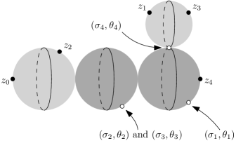
Figure 5.1. An example of the marked points from (5.1.14) (for $m=3$, $r=3$, $l=4$). The lighter shaded components are where the map $\phi$ is constant.

A point of $\mathfrak{L}_{m,r}$ represents a connected compact nodal surface $\bar{S}$ and map $\phi=(\phi_{1},\dots,\phi_{r}):\bar{S}\rightarrow{\mathbb{C}}P^{1}$, but it is worth describing that information a little more explicitly. Let’s write $\bar{S}_{1},\dots,\bar{S}_{l}$ for those irreducible components of $\bar{S}$ which form a chain connecting the marked point $z_{0}\in\bar{S}_{1}$ to $z_{m+1}\in\bar{S}_{l}$. For concreteness, let’s choose identifications $\bar{S}_{i}=\overline{{\mathbb{R}}\times S^{1}}$, so that $-\infty$ is either $z_{0}$ or the node closest to it on $\bar{S}_{i}$, and $+\infty$ is either $z_{m+1}$ or the node closest to it on $\bar{S}_{i}$. Let $p:\{1,\dots,r\}\rightarrow\{1,\dots,l\}$ be the map such that $\phi_{j}$ is non-constant precisely on $\bar{S}_{p(j)}$. We then mark the point

(5.1.14) $$(\sigma_{j},\theta_{j})=\phi_{j}^{-1}(1)\in{\mathbb{R}}\times S^{1}\subset\bar{S}_{p(j)}.$$

Note that these points can be nodes which connect $\bar{S}_{i}$ to one of the irreducible components of $\bar{S}$ which do not lie on our chain; or they can agree with one of the $(z_{1},\dots,z_{m})$; and moreover, several of those points can be the same (see Figure 5.1). The stability condition says that if some irreducible component does not contain any of the points (5.1.14), then it must have at least three other special points. The data of the stable map is completely encoded in the surface $\bar{S}$ and additional points (5.1.14).

As in the case of Deligne-Mumford space, one can modify the space by oriented real blowups, which geometrically adds relative framings at the nodes. This results in a compact manifold with corners $\mathfrak{L}_{m,r}^{\mathit{bl}}$. One can then further add framings at the marked points, which yields a principal bundle

(5.1.15) $$(S^{1})^{m+2}\longrightarrow\mathfrak{L}_{m,r}^{\operatorname{fr}}\longrightarrow\mathfrak{L}_{m,r}^{\mathit{bl}}.$$

5.2. Parameter spaces

5.2a. Fulton-MacPherson spaces

We again consider configurations $(z_{1},\dots,z_{m})$ in ${\mathbb{C}}$, for $m\geq 2$, but where now two configurations are isomorphic if they are related by a transformation $z\mapsto az+b$, with $a\in{\mathbb{R}}^{>0}$ and $b\in{\mathbb{C}}$. The interior of Fulton-MacPherson space is the parameter space

(5.2.1) $$\mathring{\mathfrak{F}}_{m}\stackrel{{\scriptstyle\mathrm{def}}}{{=}}\mathit{Conf}_{m}({\mathbb{C}})/({\mathbb{C}}\rtimes{\mathbb{R}}^{>0}).$$

The compactification $\mathfrak{F}_{m}$ is a manifold with corners, stratified as in (5.1.3):

(5.2.2) $$\mathfrak{F}_{m}=\bigsqcup_{T}\mathring{\mathfrak{F}}_{T},\quad\mathring{\mathfrak{F}}_{T}=\prod_{v}\mathring{\mathfrak{F}}_{|v|_{\operatorname{in}}}.$$

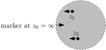
Figure 5.2. A punctured plane, with aligned asymptotic markers.

An application of Lemma 5.1.2 shows that the $\mathit{Sym}(m)$-action on $\mathfrak{F}_{m}$ is free.

Let’s choose asymptotic markers which are aligned, in following sense. At the finite $z_{i}$, markers go in negative real direction; and at $z_{0}=\infty$, the marker points in direction of the path $[0,1)\rightarrow{\mathbb{C}}P^{1}$, $s\mapsto-1/s$ (Figure 5.2). Correspondingly, the convenient choice of ends is

(5.2.3) $$[0,\infty)\times S^{1}\longrightarrow S,\;(s,t)\longmapsto z_{j}-\rho_{j}\exp(-2\pi(s+it))\;\;\text{ $\rho_{j}>0$, near $z_{j}$ ($j=1,\dots,m$);}$$

$$(-\infty,0]\times S^{1}\longrightarrow S,\;(s,t)\longmapsto\chi-\rho_{0}\exp(-2\pi(s+it))\;\;\text{ $\rho_{0}>0$, $\chi\in{\mathbb{C}}$, near $z_{0}=\infty$.}$$

These are a sub-class of rational ends, following the terminology of Section 5.1b, and compatible with our choice of asymptotic markers. This particular class of ends is preserved under gluing, hence a consistent choice can be made within it.

Remark 5.2.1.

The relation between Fulton-MacPherson and Deligne-Mumford space can be expressed in several ways. If $S=\bar{S}\setminus\{z_{0},\dots,z_{m}\}$ represents a point of $\mathfrak{F}_{m}$, then from the aligned markers, it clearly has a marker at $z_{0}$ and relative markers at the nodes; any choice of those can arise, and that is enough to determine the Fulton-MacPherson point. Additionally, the aligned condition corresponds to specific choices of markers at $(z_{1},\dots,z_{m})$. The outcome is that

(5.2.4) $$(S^{1})^{m}\times\mathfrak{F}_{m}\stackrel{{\scriptstyle\cong}}{{\longrightarrow}}\mathfrak{M}_{m}^{\operatorname{fr}},$$

where the $(S^{1})^{m}$ rotates markers at $(z_{1},\dots,z_{m})$ (this is well-known, compare e.g. the end of the proof of [39, Proposition 2.1]). The embedding $\mathfrak{F}_{m}\hookrightarrow\mathfrak{M}_{m}^{\operatorname{fr}}$ obtained by taking trivial rotations is particularly important, since it is compatible with the operad structure, or more concretely with gluing surfaces together.

5.2b. Configurations on the cylinder

Consider configurations on the cylinder (5.1.11), for some $m>0$, up to translation in ${\mathbb{R}}$-direction. The parameter space is

(5.2.5) $$\mathring{\mathfrak{C}}_{m}=\mathit{Conf}_{m}({\mathbb{R}}\times S^{1})/{\mathbb{R}}.$$

The construction of the compactification $\mathfrak{C}_{m}$ can be divided into two steps.

• One first introduces a partial compactification $\mathfrak{C}_{m}^{\heartsuit}$ where, as points on the cylinder collide, they bubble into a configuration on ${\mathbb{C}}$, determined up to ${\mathbb{C}}\rtimes{\mathbb{R}}^{>0}$. The stratification is correspondingly

  (5.2.6) $$\mathfrak{C}_{m}^{\heartsuit}=\bigsqcup_{T}\mathfrak{C}_{T}^{\heartsuit},\quad\mathfrak{C}_{T}^{\heartsuit}=\mathring{\mathfrak{C}}_{|v_{\operatorname{root}}|_{\operatorname{in}}}\times\prod_{v\neq v_{\operatorname{root}}}\mathring{\mathfrak{F}}_{|v|_{\operatorname{in}}}.$$

• The full compactification builds in breaking of the cylinder, as points go to $\pm\infty$:

  (5.2.7) $$\mathfrak{C}_{m}=\bigsqcup_{\begin{subarray}{c}l\geq 1\\ m_{1}+\cdots+m_{l}=m\end{subarray}}\mathfrak{C}_{m_{1}}^{\heartsuit}\times\cdots\times\mathfrak{C}_{m_{l}}^{\heartsuit}.$$

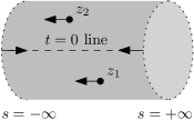
Figure 5.3. Asymptotic markers on a cylinder.

We choose $S^{1}$-invariant asymptotic markers for the punctured cylinder (see Figure 5.3). At $\pm\infty$, these point in the direction of the paths $s\mapsto(\pm 1/s,0)$, and at $z_{1},\dots,z_{m}$ they go in negative $s$-direction. Correspondingly, one picks ends

(5.2.8) $$(-\infty,0]\times S^{1}\longrightarrow S,\;\;(s,t)\longmapsto(s+\sigma_{0},t)\;\;\text{ $\sigma_{0}\in{\mathbb{R}}$, near $z_{0}=-\infty$;}$$

(5.2.9) $$[0,\infty)\times S^{1}\longrightarrow S,\;\;(s,t)\longmapsto z_{j}-\rho_{j}\exp(-2\pi(s+it))\;\;\text{ $\rho_{j}>0$, near $z_{j}$, $j=1,\dots,m$;}$$

(5.2.10) $$[0,\infty)\times S^{1}\longrightarrow S,\;\;(s,t)\longmapsto(s+\sigma_{m+1},t)\;\;\text{ $\sigma_{m+1}\in{\mathbb{R}}$, near $z_{m+1}=+\infty$.}$$

These are not rational ends in the previously defined sense, but they play a similar role of reducing the amount of choice involved. If one uses these and the previously introduced ends on Fulton-MacPherson spaces, then the whole can be made consistent with respect to both gluing processes that occur here (merging two cylinders along $\pm\infty$, as well as inserting a punctured plane at some point in a cylinder).

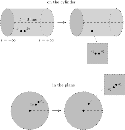
Figure 5.4. The degeneration from Remark 5.2.2.

Remark 5.2.2.

It turns out that

(5.2.11) $$\mathfrak{C}_{m}\cong\mathfrak{F}_{m+1}.$$

On the interior, take

(5.2.12) $${\mathbb{R}}\times S^{1}\stackrel{{\scriptstyle\cong}}{{\longrightarrow}}{\mathbb{C}}^{*},\quad s+it\longmapsto\exp(-2\pi(s+it))$$

This induces an isomorphism $\mathring{\mathfrak{C}}_{m}\cong\mathring{\mathfrak{F}}_{m+1}$. In terms of combinatorics, a stratum of $\mathfrak{C}_{m}$ is associated to a collection of trees $T_{1},\dots,T_{m}$. For each $i>0$, let’s turn the semi-infinite outgoing edge of each $T_{i+1}$ into a finite edge going towards the root of $T_{i}$; and add a semi-infinite edge going towards of the root of $T_{m}$. The outcome is a single tree $T$ with $(m+1)$ semi-infinite ends, which indexes the corresponding stratum of $\mathfrak{F}_{m+1}$. The problem with (5.2.11) is that it is not compatible, at least not in the most straightforward way, with writing the stratifications as products in (5.2.2) and (5.2.6). To see that, take Figure 5.4, which shows the same degeneration (two points colliding) in $\mathring{\mathfrak{C}}_{2}$ and $\mathring{\mathfrak{F}}_{3}$. This yields limits in the strata $\mathring{\mathfrak{C}}_{1}\times\mathring{\mathfrak{F}}_{2}\subset\mathfrak{C}_{2}$ respectively $\mathring{\mathfrak{F}}_{2}\times\mathring{\mathfrak{F}}_{2}\subset\mathfrak{F}_{3}$, but those limits are not obtained from each other by just applying (5.2.11) in each factor: instead, the second factor should be rotated in a way which depends on the position of the point in the first factor. For that reason, we prefer to treat $\mathfrak{C}_{m}$ and $\mathfrak{F}_{m+1}$ separately. In accordance with that distinction, our choices are framings yield embeddings $\mathfrak{F}_{m+1}\rightarrow\mathfrak{M}_{m+1}^{\operatorname{fr}}$, $\mathfrak{C}_{m}\rightarrow\mathfrak{M}_{m+1}^{\operatorname{fr}}$ with different images.

5.2c. Angle-decorated cylinders

Fix some $r>0$, and consider an $r$-tuple

(5.2.13) $$(\sigma_{1},\theta_{1}),\dots,(\sigma_{r},\theta_{r})\in{\mathbb{R}}\times S^{1},\quad\sigma_{1}\leq\cdots\leq\sigma_{r}.$$

Geometrically, one thinks of marking the cylinder $S={\mathbb{R}}\times S^{1}$ with the circles $\{s=\sigma_{i}\}$, and where each circle comes equipped with an angle $\theta_{i}$. We call this an angle-decorated cylinder. Instead of the separate angles, it can often be convenient to work with sums

(5.2.14) $$\theta_{\leq i}=\theta_{1}+\cdots+\theta_{i},\;\;\theta_{\geq i}=\theta_{i}+\theta_{i+1}+\cdots+\theta_{r},\;\;\theta_{\mathit{tot}}=\theta_{\leq r}=\theta_{\geq 1}.$$

Suppose we have two angle-decorated cylinders $S_{\pm}$. When gluing the $+\infty$ end of $S_{+}$ to the $-\infty$ end of $S_{-}$ to form a new cylinder, our convention is to always use angle-twisted gluing, which means that $(s,t)\in S_{+}$ gets identified with $(s-l,t+\theta_{\mathit{tot},-})\in S_{-}$ ($l$ is the gluing length; what’s important is the appearance of the total angle of $S_{-}$).

Write $\Sigma_{r}\subset{\mathbb{R}}^{r}$ for the space of $(\sigma_{1},\dots,\sigma_{r})$ satisfying the condition from (5.2.13). The parameter space of angle-decorated cylinders is

(5.2.15) $$\mathring{\mathfrak{A}}_{r}=(\Sigma_{r}\times(S^{1})^{r})/{\mathbb{R}}.$$

Unlike the previous situations, this already has codimension $1$ boundary faces before compactification, which occur when $\sigma_{i}=\sigma_{i+1}$ for some $i$. Those faces comes with natural maps

(5.2.16) $$\partial_{\sigma_{i+1}=\sigma_{i}}\mathring{\mathfrak{A}}_{r}\longrightarrow\mathring{\mathfrak{A}}_{r-1},$$

where we replace the adjacent pair $(s_{i},\theta_{i})$, $(s_{i+1}=s_{i},\theta_{i+1})$ with $(s_{i},\theta_{i}+\theta_{i+1})$, preserving $\theta_{\mathit{tot}}$.

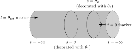
Figure 5.5. An angle-decorated cylinder.

The compactification $\mathfrak{A}_{r}$ is defined by allowing some of the $\sigma_{i}$ to go to $\pm\infty$, leading to a finite collection of cylinders of the same kind, which means that

(5.2.17) $$\mathfrak{A}_{r}=\bigsqcup_{\begin{subarray}{c}l\geq 1\\ r_{1}+\cdots+r_{l}=r\end{subarray}}\mathring{\mathfrak{A}}_{r_{1}}\times\cdots\times\mathring{\mathfrak{A}}_{r_{l}}.$$

The map $(\theta_{1},\dots,\theta_{r})$ extends smoothly to the compactification, and on each stratum (5.2.17), that extension is the product of the corresponding maps on the factors. The forgetful map (5.2.16) also extends smoothly to compactifications.

One always chooses the asymptotic marker at $+\infty$ to point in direction of $s\mapsto(1/s,0)$, but that at $-\infty$ to point in the direction of $s\mapsto(-1/s,\theta_{\mathit{tot}})$ (Figure 5.5). The ends are correspondingly taken to be

(5.2.18) $$(-\infty,0]\times S^{1}\longrightarrow S,\quad(s,t)\longmapsto(s+\sigma_{0},\,t+\theta_{\mathit{tot}}),$$

$$[0,\infty)\times S^{1}\longrightarrow S,\quad(s,t)\longmapsto(s+\sigma_{1},t)$$

As usual, one wants to make a universal choice of ends over $\mathring{\mathfrak{A}}_{r}$, consistent with angle-twisted gluing. One additionally requires that the choice of ends should be compatible with (5.2.16).

5.2d. Angle-decorated configurations

We next define parameter spaces $\mathfrak{AC}_{m,r}$, for $m+r>0$, which are a mashup of those from Section 5.2b and 5.2c. Consider configurations of $m$ marked points on the cylinder, and also data (5.2.13), both up to common translation in ${\mathbb{R}}$-direction:

(5.2.19) $$\mathring{\mathfrak{AC}}_{m,r}=\big{(}\mathit{Conf}_{m}({\mathbb{R}}\times S^{1})\times\Sigma^{r}\times(S^{1})^{r}\big{)}/{\mathbb{R}}.$$

As in (5.2.16), this space has boundary where $\sigma_{i}=\sigma_{i+1}$, and forgetful map

(5.2.20) $$\partial_{\sigma_{i+1}=\sigma_{i}}\mathring{\mathfrak{AC}}_{m,r}\longrightarrow\mathring{\mathfrak{AC}}_{m,r-1}.$$

The compactification is constructed as in Section 5.2b, by first taking

(5.2.21) $$\mathfrak{AC}_{m,r}^{\heartsuit}=\bigsqcup_{T}\mathfrak{AC}_{T}^{\heartsuit},\quad\mathfrak{AC}_{T}^{\heartsuit}=\mathring{\mathfrak{AC}}_{|v_{\operatorname{root}}|_{\operatorname{in}},r}\times\prod_{v\neq v_{\operatorname{root}}}\mathring{\mathfrak{F}}_{|v|_{\operatorname{in}}},$$

amd then

(5.2.22) $$\mathfrak{AC}_{m,r}=\bigsqcup_{\begin{subarray}{c}l\geq 1\\ m_{1}+\cdots+m_{l}=m\\ r_{1}+\cdots+r_{l}=r\end{subarray}}\mathfrak{AC}_{m_{1},r_{1}}^{\heartsuit}\times\cdots\times\mathfrak{AC}_{m_{l},r_{l}}^{\heartsuit}.$$

These identifications are chosen so that angle-twisted gluing is continuous (Figure 5.6). The outcome is a manifold with corners. One chooses asymptotic markers and ends at $\pm\infty$ as in (5.2.18); and around $(z_{1},\dots,z_{m})$ as in (5.2.9), consistently with gluing and compatibly with (5.2.20).

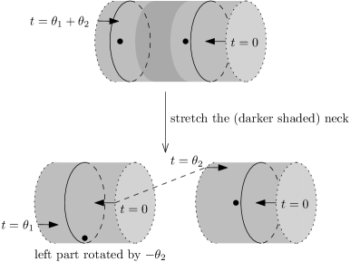
Figure 5.6. A degeneration in $\mathfrak{AC}_{2,2}$, with limit in $\mathring{\mathfrak{AC}}_{1,1}\times\mathring{\mathfrak{AC}}_{1,1}$ following (5.2.22).

Remark 5.2.3.

Starting with our choice of asymptotic markers, and then allowing those at $(z_{0},z_{1},\dots,z_{m})$ to rotate, yields an analogue of (5.2.4), namely a map into the space of framed lollipops from (5.1.15),

(5.2.23) $$(S^{1})^{m+1}\times\mathfrak{AC}_{m,r}\longrightarrow\mathfrak{L}_{m,r}^{\operatorname{fr}}.$$

These spaces in fact only differ by the condition $\sigma_{i}\leq\sigma_{i+1}$. One can show that the equality $\sigma_{i}=\sigma_{i+1}$ is transverse to all the boundary strata of $\mathfrak{L}_{m,r}^{\operatorname{fr}}$. This is one way to prove that $\mathfrak{AC}_{m,r}$ is a manifold with corners, since that reduces the question to the more familiar study of the stable map spaces that underlie the notion of lollipop.

5.2e. Cartan homotopy moduli spaces (A)

We now turn to the two spaces used to define the connection on equivariant Floer cohomology. Both are constructed inside $\mathfrak{AC}_{m,r}$, and use the same kinds of asymptotic markers and ends.

Take a configuration (5.1.11), $m>0$, with angle decorations (5.2.13). Fix some $w\in\{0,\dots,r\}$ and impose the following constraint on the first point (Figure 5.7):

(5.2.24) $$z_{1}=(s_{1},t_{1}=\theta_{\geq w+1})\;\;s_{1}\in\begin{cases}{\mathbb{R}}&r=0,\\ (-\infty,\sigma_{1}]&w=0,\,r>0\\ [\sigma_{w},\sigma_{w+1}]&w=1,\dots,r-1,\\ [\sigma_{r},\infty)&w=r,\,r>0\end{cases}$$

The space of those, up to ${\mathbb{R}}$-translation, is written as $\mathring{\mathfrak{AC}}_{m,r,w}^{(A)}$. This has different kinds of codimension $1$ boundary faces:

• We can have $\sigma_{i}=\sigma_{i+1}$ for some $i\neq w$ (the $i=w$ case is of codimension $2$, hence not listed here). Those faces comes with the usual map (note that the forgetting process is compatible with the condition that $t_{1}=\theta_{\geq w+1}$)

  (5.2.25) $$\partial_{\sigma_{i}=\sigma_{i+1}}\mathring{\mathfrak{AC}}_{m,r,w}^{(A)}\longrightarrow\begin{cases}\mathring{\mathfrak{AC}}_{m,r,w-1}^{(A)}&i<w,\\ \mathring{\mathfrak{AC}}_{m,r,w}^{(A)}&i>w.\end{cases}$$

• We can have $s_{1}=\sigma_{w}$ (when $w\neq 0$) or $s_{1}=\sigma_{w+1}$ (when $w\neq r$). Those boundary faces are written as $\partial_{s_{1}=\sigma_{w}}\mathring{\mathfrak{AC}}_{m,r,w}^{(A)}$, $\partial_{s_{1}=\sigma_{w+1}}\mathring{\mathfrak{AC}}_{m,r,w}^{(A)}$.

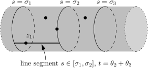
Figure 5.7. The position constraint from (5.2.24).

Clearly, $\mathring{\mathfrak{AC}}_{m,r,w}^{(A)}$ is a codimension $1$ submanifold with boundary in $\mathring{\mathfrak{AC}}_{m,r}$. We define $\mathfrak{AC}_{m,r,i}^{(A)}$ to be its closure in $\mathfrak{AC}_{m,r}$. Concretely, this means that one has a partial compactification $\mathfrak{AC}_{m,r,w}^{(A),\heartsuit}$ as in (5.2.21), and then the analogue of (5.2.22) is

(5.2.26) $$\mathfrak{AC}_{m,r,w}^{(A)}=\bigsqcup\,\mathfrak{AC}_{m_{1},r_{1}}^{\heartsuit}\times\cdots\times\mathfrak{AC}_{m_{k},r_{k},w-r_{1}-\cdots-r_{k-1}}^{(A),\heartsuit}\times\cdots\times\mathfrak{AC}_{m_{l},r_{l}}^{\heartsuit}.$$

The union is over all $l\geq 1$, $m_{1}+\cdots+m_{l}=m$, $r_{1}+\cdots+r_{l}=r$, and $1\leq k\leq l$ such that the spaces in the formula make sense. This closure is a submanifold with corners inside $\mathfrak{AC}_{m,r}$. The main point here is that $\theta_{\geq w+1}$ extends to a function on $\mathfrak{AC}_{m,r}$ without any critical points, and the same for its restriction to any closed stratum; hence setting $t_{1}=\theta_{\geq w+1}$ is automatically a transverse constraint, even though $t_{1}$ does have critical points. The same applies to the other part of (5.2.24) in a slightly more complicated way (one can use translation-invariance to fix $s_{1}=0$, and then the constraints become $\sigma_{w}\leq 0$, $\sigma_{w+1}\geq 0$). The compactification has additional codimension $1$ boundary faces:

• The cylinder can split into two, with the part carrying $z_{1}$ lying either on the left of right. This is the case $l=2$ of (5.2.26), which means that the open stratum is

  (5.2.27) $$\mathring{\mathfrak{AC}}_{m_{1},r_{1}}\times\mathring{\mathfrak{AC}}_{m_{2},r_{2},w-r_{1}}^{(A)}\;\;\text{ or }\;\;\mathring{\mathfrak{AC}}_{m_{1},r_{1},w}^{(A)}\times\mathring{\mathfrak{AC}}_{m_{2},r_{2}},\;\;m_{1}+m_{2}=m,\;r_{1}+r_{2}=r.$$

• We can have Fulton-MacPherson bubbling, where a group of punctures collide. Strictly speaking, there are two sub-cases here, depending on whether $z_{1}$ ends up on the bubble of not.

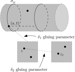
Figure 5.8. The gluing process from Remark 5.2.4.

Remark 5.2.4.

To further illustrate the submanifold-with-corners structure, it is useful to look at the coordinates given by the gluing process. Take a stratum in (5.2.21) where two levels of Fulton-MacPherson bubbling have occurred at a point on the $\sigma_{w}$ circle, and where the point $z_{1}\in{\mathbb{C}}$ lies on one of the resulting bubbles, as in Figure 5.8. Write $z\in{\mathbb{C}}$ and $(s,t)\in{\mathbb{R}}\times S^{1}$ for the relevant attaching points (which can move as part of the parameter space, as can $z_{1}$). After gluing the surfaces together using parameters $\gamma_{1},\gamma_{2}>0$ (suppressing some irrelevant constants), the point $z_{1}$ would end up at $(s,t)+\gamma_{1}(z+\gamma_{2}z_{1})\in{\mathbb{R}}\times S^{1}$. Then, (5.2.24) is given by the following conditions on $(\gamma_{1},\gamma_{2},\sigma_{w},s,t,z,z_{1})$:

(5.2.28) $$s+\gamma_{1}\mathrm{re}(z)+\gamma_{1}\gamma_{2}\mathrm{re}(z_{1})\geq\sigma_{w},$$

$$t+\gamma_{1}\mathrm{im}(z)+\gamma_{1}\gamma_{2}\mathrm{im}(z_{1})=\theta_{\geq w+1}.$$

As one can see, if one turns the first into an equality, it is always transversally cut out at $\gamma_{1}=\gamma_{2}=0$; and so is the second one.

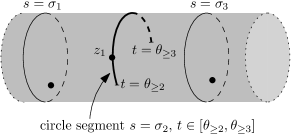
Figure 5.9. The position constraint from (5.2.29).

5.2f. Cartan homotopy moduli spaces (B)

We start with a cylinder configuration as before, some $r\geq 1$ and $1\leq w\leq r$. As part of the data, we include a lift of $\theta_{w}$ to $[0,1]$, and an extra variable $\xi$, which are enter into the position constraint for $z_{1}$ (Figure 5.9 shows a slightly simplified picture of the outcome):

(5.2.29) $$\theta_{w}^{\operatorname{lift}}\in[0,1],\;\;\xi\in[\theta_{w}^{\operatorname{lift}},1],\quad z_{1}=(s_{1}=\sigma_{w},\,t_{1}=\theta_{\geq w+1}+\xi).$$

The resulting parameter space $\mathring{\mathfrak{AC}}_{m,r,w}^{(B)}$ has the following codimension $1$ boundary faces:

• The by now standard ones where $\sigma_{i}=\sigma_{i+1}$ for some $i$. In the cases where $i=w-1$ and $i=w$, the forgetful maps should be thought of as ignoring the condition on $t_{1}$, which means they have the form

  (5.2.30) $$\partial_{\sigma_{w-1}=\sigma_{w}}\mathring{\mathfrak{AC}}_{m,r,w}^{(B)}\longrightarrow\{\text{subset of $\mathring{\mathfrak{AC}}_{m,r-1}$ where $z_{1}=(s_{1},t_{1})$, $s_{1}=\sigma_{w-1}$}\},$$

  $$\partial_{\sigma_{w}=\sigma_{w+1}}\mathring{\mathfrak{AC}}_{m,r,w}^{(B)}\longrightarrow\{\text{subset of $\mathring{\mathfrak{AC}}_{m,r-1}$ where $z_{1}=(s_{1},t_{1})$, $s_{1}=\sigma_{w}$}\}.$$

  It is still true that they decrease dimensions, which is what’s important for us.

• We can have $t_{1}=\theta_{\geq w}$. This comes with a map to one of the boundary faces of the (A) type spaces,

  (5.2.31) $$\partial_{t_{1}=\theta_{\geq w}}\mathring{\mathfrak{AC}}_{m,r,w}^{(B)}\longrightarrow\partial_{s_{1}=\sigma_{w}}\mathring{\mathfrak{AC}}_{m,r,w-1}^{(A)},$$

  which is an isomorphism away from a subset of positive codimension (the issue being the lifts to $[0,1]$ in (5.2.29), which carry nontrivial information only at the endpoints $\{0,1\}$). At the other extreme, we can have $t_{i}=\theta_{\geq w+1}$, and a parallel map

  (5.2.32) $$\partial_{t_{1}=\theta_{\geq w+1}}\mathring{\mathfrak{AC}}_{m,r,w}^{(B)}\longrightarrow\partial_{s_{1}=\sigma_{w}}\mathring{\mathfrak{AC}}_{m,r,w}^{(A)}.$$

• Finally, if $\theta_{w}^{\operatorname{lift}}=0$, then $t_{1}$ can lie anywhere on the circle $\{s=\sigma_{w}\}$. We can forget $\sigma_{w}$, and then the condition is that $z_{1}$ can lie anywhere in the annulus $[\sigma_{w-1},\sigma_{w+1}]\times S^{1}$. Renumbering of the angle decorations therefore yields a map

  (5.2.33) $$\partial_{\theta_{i}^{\operatorname{lift}}=0}\mathring{\mathfrak{AC}}_{m,r,w}^{(B)}\longrightarrow\mathring{\mathfrak{AC}}_{m,r-1}.$$

  The image of this is the subset of configurations decorated with $(r-1)$ angles, such that $z_{1}$ lies in the annulus $[\sigma_{w-1},\sigma_{w}]\times S^{1}$.

As before we have a compactification $\mathfrak{AC}_{m,r,w}^{(B)}$, which contributes the same additional codimension $1$ boundary strata (cylinder-breaking, bubbling off of Fulton-MacPherson configuration) as in the (A) type situation.

5.2g. Orientation conventions

We end by listing our conventions for choosing orientations on the main parameter spaces.

• For every configuration $(z_{1},\dots,z_{m})$ there is a short exact sequence

  (5.2.34) $$0\rightarrow{\mathbb{C}}\oplus{\mathbb{R}}\longrightarrow{\mathbb{C}}^{m}\longrightarrow T_{[z_{1},\dots,z_{m}]}\mathring{\mathfrak{F}}_{m}\rightarrow 0,$$

  where $1\in{\mathbb{C}}$ is mapped to $(1,\dots,1)$, and $1\in{\mathbb{R}}$ to $(-z_{1},\dots,-z_{m})$ (infinitesimal shrinking of a configuration). We use the orientation of $\mathfrak{F}_{m}$ compatible with that sequence. Let’s illustrate the example $m=2$: there, the left hand side of (5.2.34) gives three linearly independent elements in ${\mathbb{C}}^{2}$, which are naturally completed to an oriented basis

  (5.2.35) $$(1,1),\,(i,i),\,(-z_{1},-z_{2}),\,(-iz_{1},-iz_{2})\in{\mathbb{C}}^{2}.$$

  The relative angle $\alpha(z_{1},z_{2})=\arg(z_{2}-z_{1})$ satisfies $\alpha^{\prime}_{(z_{1},z_{2})}(-iz_{1},-iz_{2})=-1$, hence induces an orientation-reversing diffeomorphism $\mathfrak{F}_{2}\cong S^{1}$.

  Note that by definition, $\mathit{Sym}_{m}$ acts orientation-preservingly. One can also check that the inclusions of boundary faces

  (5.2.36) $$\mathring{\mathfrak{F}}_{m_{2}}\times\mathring{\mathfrak{F}}_{m_{1}}\hookrightarrow\partial\mathfrak{F}_{m},\;\;m=m_{1}+m_{2}-1$$

  are compatible with orientations. Here, in terms of (5.2.2), $\mathfrak{F}_{m_{1}}$ corresponds to the root vertex of the tree, so we are ordering the factors in (5.2.36) branch-to-root (the use of this ordering, specifically for orientation purposes, is motivated by the bottom left entry in Figure 5.10, where it appears naturally).

• The orientation of $\mathfrak{F}_{m+1}$ carries over to $\mathfrak{C}_{m}$ via (5.2.11). More directly, this orientation is given by the short exact sequence

  (5.2.37) $$0\rightarrow{\mathbb{R}}\longrightarrow{\mathbb{C}}^{m}\longrightarrow T_{[z_{1},\dots,z_{m}]}\mathring{\mathfrak{C}}_{m}\rightarrow 0,$$

  where $1\in{\mathbb{R}}$ is mapped to $(1,\dots,1)$ (because the marked point $z_{0}$ is now at $-\infty$, and our previous sign convention was to move away from $z_{0}$). Again, it is instructive to look at the simplest case $m=1$: there, an oriented basis of $T_{z}\mathring{\mathfrak{C}}_{1}$ is obviously given by $(1,0)$ and $(0,1)$, which means that $\mathrm{im}(z_{1})$ gives an orientation-preserving diffeomorphism $\mathfrak{C}_{1}\cong S^{1}$.

  As before, this will cause the orientations to be compatible with the inclusions of faces $\mathring{\mathfrak{C}}_{m_{2}}\times\mathring{\mathfrak{C}}_{m_{1}}\hookrightarrow\partial\mathfrak{C}_{m_{1}+m_{2}}$, (note the ordering of components is from $s=+\infty$ to $s=-\infty$, which agrees with our convention for Fulton-MacPherson spaces). The same holds for faces $\mathring{\mathfrak{F}}_{m_{2}}\times\mathring{\mathfrak{C}}_{m_{1}}\hookrightarrow\partial\mathfrak{C}_{m_{1}+m_{2}-1}$.

• For angle-decorated cylinders, we group each $(\sigma_{k},\theta_{k})$ into a complex number, and use the sequence parallel to (5.2.37),

  (5.2.38) $$0\rightarrow{\mathbb{R}}\longrightarrow{\mathbb{C}}^{r}\longrightarrow T_{[\sigma_{1},\theta_{1},\dots,\sigma_{r},\theta_{r}]}\mathring{\mathfrak{A}}_{r}\rightarrow 0.$$

  As in the previous cases, this is compatible with boundary faces. The same principle is used for angle-decorated configurations.

• For type (A) Cartan homotopy moduli spaces (Section 5.2e), we orient the line on which the first marked point lies towards the right (away from $z_{0}=-\infty$). The other marked points and angle decorations are treated as before, and we orient these moduli spaces by the resulting exact sequence:

  (5.2.39) $$0\rightarrow{\mathbb{R}}\longrightarrow{\mathbb{R}}\oplus{\mathbb{C}}^{m+r-1}\longrightarrow T_{[(\sigma_{i},\theta_{i}),z_{1},\dots,z_{m}]}\mathring{\mathfrak{AC}}_{m,r,w}^{(A)}\rightarrow 0.$$

  In the simplest case $\mathring{\mathfrak{AC}}_{1,0,0}^{(A)}=\{\mathit{point}\}$, this convention counts that point as $+1$. In general, this is the same as the orientation obtained by breaking the translational symmetry to set $z_{1}=(0,\theta_{\geq w+1})$, and then treating the remaining $z_{k}$ and $(\sigma_{k},\theta_{k})$ as complex numbers.

  Yet another equivalent description would be to say that the map $\mathring{\mathfrak{AC}}_{m,r,w}^{(A)}\times S^{1}\rightarrow\mathring{\mathfrak{AC}}_{m,r}$, where the $S^{1}$ factor rotates the second component of $z_{1}=(s_{1},t_{1})$, is compatible with orientations. This point of view is particularly convenient for considering compatibility with boundary orientations, since it reduces that question to the previously discussed cases. It turns out that (again with factors ordered from $s=+\infty$ to $s=-\infty$)

  (5.2.40) $$\mathring{\mathfrak{AC}}_{m_{2},r_{2},w-r_{1}}^{(A)}\times\mathring{\mathfrak{AC}}_{m_{1},r_{1}}\hookrightarrow\partial\mathring{\mathfrak{AC}}_{m_{1}+m_{2},r_{1}+r_{2},w}^{(A)}\text{ is orientation-reversing;}$$

  (5.2.41) $$\mathring{\mathfrak{AC}}_{m_{2},r_{2}}\times\mathring{\mathfrak{AC}}_{m_{1},r_{1},w}^{(A)}\hookrightarrow\partial\mathring{\mathfrak{AC}}_{m_{1}+m_{2},r_{1}+r_{2},w}^{(A)}\text{ is orientation-preserving;}$$

  (5.2.42) $$\mathring{\mathfrak{F}}_{m_{2}}\times\mathring{\mathfrak{AC}}_{m_{1},r,w}^{(A)}\hookrightarrow\partial\mathring{\mathfrak{AC}}_{m_{1}+m_{2}-1,r,w}^{(A)}\text{ is orientation-preserving.}$$

  (The orientation-reversal happens because one has to swap the extra $S^{1}$ factor with $\mathring{\mathfrak{AC}}_{m_{1},r_{1}}$ in the ordering, and both are odd-dimensional.)

• For type (B) Cartan homotopy moduli spaces (Section 5.2f) we orient the circle on which $z_{1}$ lies counterclockwise, meaning in direction of increasing $t_{1}$. This gives rise to an analogous exact sequence which we use to orient the moduli spaces:

  (5.2.43) $$0\rightarrow{\mathbb{R}}\longrightarrow{\mathbb{R}}\oplus{\mathbb{C}}^{m+r-1}\longrightarrow T_{[(\sigma_{i},\theta_{i}),z_{1},\dots,z_{m}]}\mathring{\mathfrak{AC}}_{m,r,w}^{(B)}\rightarrow 0.$$

  Equivalently, one can say that the map $\mathring{\mathfrak{AC}}_{m,r,w}^{(B)}\times{\mathbb{R}}\rightarrow\mathring{\mathfrak{AC}}_{m,r}$, where ${\mathbb{R}}$ translates the first component of $z_{1}=(s_{1},t_{1})$ to the left, is compatible with orientations. For the boundary faces parallel to those in (5.2.40)–(5.2.42), we get the same orientation behaviour.

  There is an additional boundary face, which appears in the forgetful map (5.2.33). Let’s consider the simplest case $m=r=w=1$. The space ${\mathbb{R}}\oplus{\mathbb{C}}$ in the middle of (5.2.43) is oriented according to the coordinates $(t_{1},\sigma_{1},\theta_{1}^{\mathrm{lift}})$, and since $\theta_{1}^{\mathrm{lift}}=0$ is the minimal value of that coordinate, the resulting boundary face is ordered opposite to $(t_{1},\sigma_{1})$, or equivalently agrees with the orientation from $(\sigma_{1},t_{1})$. The forgetful map corresponds to considering $(\sigma_{1},t_{1})$ as a complex number, and is accordingly orientation-preserving. The same is true in general.

5.3. Closed string operations

5.3a. $L_{\infty}$-structure

We are now ready to construct the operations on symplectic cohomology, following the general framework laid out in Section 4.1g. Take $\hat{N}$ as in (4.1.10), (4.1.38). We also fix $(H,J)$ which sets up the Floer complex (Section 4.1e).

We begin by introducing operations parameterized by the spaces $\mathfrak{F}_{m}$ (Section 5.2a) for each $m\geq 2$. We suppose that a universal family of cylindrical ends (5.2.3) on each $\mathring{\mathfrak{F}}_{m}$ has been fixed, consistently with gluing. We also choose families of Hamiltonian perturbations and almost complex structures on the universal curves,

(5.3.1) $$K_{\mathfrak{F}_{m}}\in\Omega^{1}_{U_{\mathfrak{F}_{m}}/\mathfrak{F}_{m}}(U_{\mathfrak{F}_{m}},\mathcal{H}(\hat{N}))\text{ and }J_{\mathfrak{F}_{m}}\in C^{\infty}(U_{\mathfrak{F}_{m}},\mathcal{J}(\hat{N})),$$

which satisfy the conditions of Section 4.1f when restricted to each point in parameter space, are conformally consistent with respect to boundary strata in the sense of Section 4.1h, and are equivariant with respect to the $\mathit{Sym}(m)$-action.

Remark 5.3.1.

The equivariance constraint is unproblematic for transversality, because the action on $\mathring{\mathfrak{F}}_{m}$ is free. More concretely, any point in $\mathring{\mathfrak{F}}_{m}$ has a neighbourhood $U$ which is disjoint from its image $\sigma(U)$ under any nontrivial $\sigma\in\mathit{Sym}(m)$. On such a $U$, equivariance does not restrict the choice of (5.3.1), and since regularity of the parametrized moduli space is a local property over the parameter space, that suffices. Equivalently, one can think of regularity being achieved over the quotient $\mathring{\mathfrak{F}}_{m}/\mathit{Sym}(m)$.

Let $\mathring{\mathfrak{F}}_{m}(\mathbf{x})=\mathring{\mathfrak{F}}_{m}(x_{0},\dots,x_{m})$ be the parametrized moduli space of maps satisfying the Cauchy-Riemann equations, and with fixed asymptotics (this follows the general notation from Section 4.1g). For generic choice of (5.3.1), this is a manifold of the expected dimension

(5.3.2) $$\operatorname{dim}\,\mathring{\mathfrak{F}}_{m}(\mathbf{x})=\deg(x_{0})-\sum_{i=1}^{m}(\deg(x_{i}))+2m-3.$$

Following (4.1.69), each point $(r,u)$ in this space gives rise to an isomorphism

(5.3.3) $$o(r,u):\lambda^{\mathrm{top}}(T_{(r,u)}\mathring{\mathfrak{F}}_{m}(\mathbf{x}))\otimes\mathfrak{o}_{x_{1}}\otimes\cdots\otimes\mathfrak{o}_{x_{m}}\cong\lambda^{\mathrm{top}}(T_{r}\mathring{\mathfrak{F}}_{m})\otimes\mathfrak{o}_{x_{0}}.$$

The spaces $\mathring{\mathfrak{F}}_{m}(\mathbf{x})$ have Gromov compactifications

(5.3.4) $$\mathfrak{F}_{m}(\mathbf{x})=\bigsqcup_{T}\mathfrak{F}_{T}(\mathbf{x})$$

whose strata are indexed by trees $T$ similar to (5.2.2), but allowing unstable vertices with $|v|_{\mathrm{in}}=1$, which correspond to breaking off of positive energy Floer cylinders. When the expected dimension (5.3.2) is $0$, all strata except the interior are empty, hence $\mathring{\mathfrak{F}}_{m}(\mathbf{x})=\mathfrak{F}_{m}(\mathbf{x})$ is a finite set. Via (5.3.3) and the orientation of $\mathfrak{F}_{m}$ from Section 5.2g, each point in that set gives an isomorphism $\mathfrak{o}_{x_{1}}\otimes\cdots\otimes\mathfrak{o}_{x_{m}}\cong\mathfrak{o}_{x_{0}}$. We add up the ${\mathbb{K}}$-normalization of those isomorphisms to obtain the operation

(5.3.5) $$\ell^{m}:\mathit{CF}^{*}(H)^{\otimes m}\longrightarrow\mathit{CF}^{*+3-2m}(H).$$

On $\mathcal{G}=\mathit{CF}^{*}(H)[1]$, the degree of these operations becomes $2-m$. We extend them to $m=1$ by declaring $\ell^{1}$ to be the Floer differential. The fact that our perturbation data are equivariant implies that our operations satisfy the symmetry property (3.4.2). (Because $\mathcal{G}$ is the shifted Floer complex, the signs from (3.4.2) are $(-1)^{\|x_{k}\|}=(-1)^{\mathrm{deg}(x_{k})}$, which agrees with their geometric origin as Koszul signs associated to permuting the orientation operators $D_{x_{k}}$.)

Proposition 5.3.2.

The operations (5.3.5) define an $L_{\infty}$-structure on $\mathit{CF}^{*}(H)[1]$.

Proof.

To check that these operations satisfy the $L_{\infty}$-relations (3.4.3), we follow the standard pattern of considering one-dimensional spaces $\mathfrak{F}_{m}(\mathbf{x})$. In this case, for a generic choice of perturbation data, all nonempty boundary strata $\mathfrak{F}_{T}(\mathbf{x})$ correspond to trees with exactly two vertices (and one internal edge). Concretely, these boundary terms are of two kinds:

• ($T$ unstable, which means that one of the vertices has $|v|_{\mathrm{in}}=1$) This corresponds to cylindrical breaking-off of a Floer trajectory for $H$, meaning the strata are

  (5.3.6) $$\mathring{\mathfrak{C}}(x_{0},y_{0})\times\mathring{\mathfrak{F}}_{m}(y_{0},x_{1},\cdots,x_{m})\text{ or }\mathring{\mathfrak{F}}_{m}(x_{0},x_{1},\cdots,y_{i},\cdots,x_{m})\times\mathring{\mathfrak{C}}(y_{i},x_{i}).$$

  Here, as in Section 4.1d, $\mathring{\mathfrak{C}}(x_{0},y_{0})$ and $\mathring{\mathfrak{C}}(y_{i},x_{i})$ denote spaces of Floer trajectories up to ${\mathbb{R}}$-translation.

• ($T$ stable) The other kind of boundary strata correspond to a degeneration to a codimension $1$ stratum in $\partial\mathfrak{F}_{m}$. After applying the action of the symmetric group, these strata can be identified with

  (5.3.7) $$\mathring{\mathfrak{F}}_{m_{1}}(x_{0},y,x_{\sigma(m_{2}+1)},\dots,x_{\sigma(m)})\times\mathring{\mathfrak{F}}_{m_{2}}(y,x_{\sigma(1)},\dots,x_{\sigma(m_{2})}),\;\;m_{1}+m_{2}=m+1,$$

  for some $m_{2}$-shuffle $\sigma$, see (3.4.1), and one-periodic orbit $y$.

There is an obvious bijection between these boundary strata and terms in (3.4.3). (The stable trees correspond to compositions of operations of arity $\geq 2$; and the remaining ones to terms involving the differential $\ell^{1}.$) Standard gluing constructions show that such points correspond bijectively to ends of $\mathring{\mathfrak{F}}_{m}(\mathbf{x})$, with the correspondence given by Gromov convergence. This means that $\mathfrak{F}_{m}(\mathbf{x})$ is at least topologically a compact one-manifold with boundary, allowing for the usual “signed count of boundary points is zero” argument to go through.

The signs in the argument deserve a short discussion. To make that more transparent, we temporarily take a moduli space $\mathfrak{F}_{m}(\mathbf{x})$ of arbitrary dimension, while still considering only boundary faces of the form (5.3.7); in fact, for simplicity we will assume that $\sigma$ is trivial. Start with a point on that boundary face, given by a pair $(p_{1},u_{1}),(p_{2},u_{2})$, and let $(p,u)$ be the result of applying gluing, for some small value of the gluing parameter. We have isomorphisms

(5.3.8) $${\mathbb{R}}\oplus T_{p_{2}}\mathring{\mathfrak{F}}_{m_{2}}\oplus T_{p_{1}}\mathring{\mathfrak{F}}_{m_{1}}\cong T_{p}\mathring{\mathfrak{F}}_{m}$$

and

(5.3.9) $${\mathbb{R}}\oplus T_{(p_{1},u_{1})}\mathring{\mathfrak{F}}_{m_{1}}(x_{0},y,x_{m_{2}+1},\dots,x_{m})\oplus T_{(p_{2},u_{2})}\mathring{\mathfrak{F}}_{m_{2}}(y,x_{1},\dots,x_{m_{2}})\cong T_{(p,u)}\mathring{\mathfrak{F}}_{m}(\mathbf{x}),$$

which are not quite unique, but well-defined enough to allow us to carry over orientations. Both are obtained from linearized gluing: on the level of parameter spaces, for (5.3.8) (where the ordering follows the conventions from Section 5.2g, so that we can quote the results from there); and for parametrized moduli spaces, in the case of (5.3.9) (where the standard ordering for gluing of determinant lines is used, as in Section 4.1g). In both cases, ${\mathbb{R}}$ corresponds to the gluing parameter. The resulting isomorphisms of top exterior powers are compatible with each other via (4.1.65) and (4.1.67). By that, we mean that the diagram of one-dimensional vector spaces and isomorphisms shown in Figure 5.10 is commutative (up to multiplication with positive numbers, as usual).

To simplify the discussion, let’s suppose temporarily that identifications $\mathfrak{o}_{x_{k}}\cong{\mathbb{R}}$ have been chosen. Together with the orientations of Fulton-MacPherson spaces, this determines orientations of $\mathring{\mathfrak{F}}_{m}(\mathbf{x})$, as an instance of (4.1.65). Recall from Section 5.2g that the orientations of Fulton-MacPherson spaces are compatible with $\mathring{\mathfrak{F}}_{m_{2}}\times\mathring{\mathfrak{F}}_{m_{1}}\subset\partial\mathfrak{F}_{m}$. The commutativity of the diagram in Figure 5.10 then shows that the resulting orientations of the parametrized moduli spaces are compatible with $\mathring{\mathfrak{F}}_{m_{2}}\times\mathring{\mathfrak{F}}_{m_{1}}\subset\partial\mathfrak{F}_{m}$, up to the Koszul sign arising from the “swap”. In the case relevant to our argument, that sign is trivial, since one of the factors is zero-dimensional. This geometric result translates algebraically into the absence of signs in the term

(5.3.10) $$\ell^{m_{1}}(\ell^{m_{2}}(x_{1},\dots,x_{m_{2}}),x_{m_{2}+1},\dots,x_{m})$$

of the $L_{\infty}$-relation (3.4.3). To get the general statement from this, one only needs to add Koszul signs corresponding to permutations of the $x_{k}$. ∎

Figure 5.10. The diagram for the sign considerations in Proposition 5.3.2.

5.3b. $L_{\infty}$-module structure

We next consider the parameter spaces $\mathring{\mathfrak{C}}_{m}$ from Section 5.2b. Recall that this moduli space has been equipped with a universal choices of positive cylindrical ends at $z_{m+1}=+\infty$ and intermediate punctures $z_{1},\dots,z_{m}$, and a negative end at $z_{0}=-\infty$, as in (5.2.8)-(5.2.10). Again, we choose a family of perturbation data which is chosen within our allowed class from Section 4.1f, conformally consistent with respect to boundary strata, and $\mathit{Sym}(m)$-equivariant (note that part of consistency involves our previous choices for the $\mathcal{F}_{m}$ parameter spaces).

Let $\mathbf{x}=(x_{0},x_{1},\cdots,x_{m},x_{m+1})$ be a collection of orbits. Following our usual notational habits, we write $\mathring{\mathfrak{C}}_{m}(\mathbf{x})$ for the parameterized moduli space of solutions. These spaces generically have dimension

(5.3.11) $$\operatorname{dim}(\mathring{\mathfrak{C}}_{m}(\mathbf{x}))=\operatorname{deg}(x_{0})-\sum_{i=1}^{m+1}\operatorname{deg}(x_{i})+2m-1.$$

Counting points in zero-dimensional moduli spaces then gives rise to operations of degree $1-m$,

(5.3.12) $$\ell^{m,1}:(\mathit{CF}^{*}(H[1])^{\otimes m})\otimes\mathit{CF}^{*}(H)\longrightarrow\mathit{CF}^{*}(H)$$

Proposition 5.3.3.

The operations $\ell^{m,1}$ give $\mathit{CF}^{*}(H)$ the structure of an $L_{\infty}$-module over $\mathit{CF}^{*}(H)[1].$

Proof.

The proof again proceeds by examining the boundaries of one-dimensional moduli spaces $\mathfrak{C}_{m}(\mathbf{x})$. There are two possible boundary types to consider:

• The first is where we have a degeneration to a codimension $1$ boundary of (5.2.6) (meaning we have a Fulton-MacPherson configuration bubbling off at one of the interior marked points) or a breaking of a Floer trajectory at one of the points $z_{1},\dots,z_{m}$. These correspond to the first sum on the right-hand side of (3.4.9).

• The second possible degeneration is a cylindrical breaking at $\pm\infty$. This means either an ordinary Floer breaking

  (5.3.13) $$\mathfrak{C}(x_{0},y_{0})\times\mathfrak{C}_{m}(y_{0},x_{1},\dots,x_{m},x_{\infty})\text{ or }\mathfrak{C}_{m}(x_{0},x_{1},\dots,x_{m},y_{\infty})\times\mathfrak{C}(y_{\infty},x_{\infty});$$

  or else, that the domain degenerates to the boundary of $\mathfrak{C}_{m}$, so that we have a limit

  (5.3.14) $$(p_{1},u_{1},p_{2},u_{2})\in\mathring{\mathfrak{C}}_{m_{1}}\times\mathring{\mathfrak{C}}_{m_{2}},\quad m_{1}+m_{2}=m.$$

  This boundary type accounts for the second sum in (3.4.9).

The verification that these boundary strata contribute with the correct signs proceeds as in Lemma 5.3.2 (details omitted). ∎

Remark 5.3.4.

As noted in Example 3.4.2, one can also consider the “diagonal” module $M=\mathit{CF}^{*}(H)$ over $\mathcal{G}=\mathit{CF}^{*}(H)[1]$ with operations $\ell^{m,1}\stackrel{{\scriptstyle\mathrm{def}}}{{=}}\ell^{m+1}$. However, the module structure defined by the operations (5.3.12) is in general different from the diagonal one, due to the fact that we have chosen $S^{1}$-invariant markers over $\mathfrak{C}_{m}$ as opposed to aligned markers over $\mathfrak{F}_{m+1}$ (compare Remark 5.2.2). This will later on lead to two versions of $q$-deformed Floer groups.

5.3c. $S^{1}$-equivariant Floer groups

The definition of the $S^{1}$-equivariant Floer complex involves parametrized operations over the spaces $\mathring{\mathfrak{A}}_{r}$ (Section 5.2c; a version of this approach is used in [32]). Recall that the ends are chosen to be of the form (5.2.18)(in particular, the negative puncture at $s=-\infty$ is rotated by $\theta^{\operatorname{tot}}$) and compatible with the map (5.2.16) over the boundary $\partial_{\sigma_{i+1}=\sigma_{i}}\mathfrak{A}_{r}$. We choose perturbation data for each fiber of the universal curve (still within the class from Section 4.1f) which over $\partial_{\sigma_{i+1}=\sigma_{i}}\mathfrak{A}_{r}$:

(5.3.15) $$\text{coincide with the pull-back of the data chosen over }\mathring{\mathfrak{A}}_{r-1}.$$

Of course, we also require these perturbations to be chosen conformally consistently over boundary strata. For any pair of orbits $x_{0},x_{1}$, we let $\mathring{\mathfrak{A}_{r}}(x_{0},x_{1})$ denote the moduli space of parameterized solutions for these choices. This has virtual dimension

(5.3.16) $$\operatorname{dim}(\mathring{\mathfrak{A}_{r}}(x_{0},x_{1}))=\operatorname{deg}(x_{0})-\operatorname{deg}(x_{1})+2r-1$$

and hence after choosing perturbation data generically, rigid moduli spaces give rise to operations

(5.3.17) $$\delta_{S^{1}}^{r}:\mathit{CF}^{*}(H)\longrightarrow\mathit{CF}^{*+1-2r}(H)$$

for any $r\geq 1$. In the degenerate case where $r=0$, we define $\delta_{S^{1}}^{0}=\delta$ to be the already defined Floer differential.

Lemma 5.3.5.

For any $r\geq 0$,

(5.3.18) $$\sum_{j=0}^{r}\delta_{S^{1}}^{j}\delta_{S^{1}}^{r-j}=0.$$

Proof.

Examining the boundary of compactified one-dimensional moduli spaces (keeping the orientation computations from Section 5.2g in mind) immediately gives

(5.3.19) $$\sum_{j=0}^{r}\delta_{S^{1}}^{j}\delta_{S^{1}}^{r-j}+\sum_{i}\delta^{r}_{i,i+1}=0.$$

Here $\delta^{r}_{i,i+1}$ denotes the contributions from curves lying over the boundary strata $\partial_{\sigma_{i+1}=\sigma_{i}}\mathfrak{A}_{r}.$ However, the consistency condition (5.3.15) implies that the Floer datum chosen for any element $C_{r}$ for $r\in\partial_{\sigma_{i+1}=\sigma_{i}}\mathfrak{A}_{r}$ only depends on its image under the forgetful map to $\mathring{\mathfrak{A}}_{r-1}$. As this forgetful map has one dimensional fibers, there can be no rigid curves lying over those strata. Thus all of the $\delta^{r}_{i,i+1}$ vanish, yielding (5.3.18). ∎

The equivariant Floer complex is the ${\mathbb{Z}}$-graded complex of ${\mathbb{K}}[[u]]$-modules

(5.3.20) $$\mathit{CF}_{S^{1}}^{*}(H)\stackrel{{\scriptstyle\mathrm{def}}}{{=}}\mathit{CF}^{*}(H)[[u]],\quad\delta_{S^{1}}=\sum_{r=0}^{\infty}u^{r}\delta_{S^{1}}^{r}.$$

5.3d. $S^{1}$-equivariant $L_{\infty}$-module structure

Here we consider the operations governed by parameterized Floer theory over $\mathring{\mathfrak{AC}}_{m,r}$ from Section 5.2d. The universal ends at $s=\pm\infty$ are chosen as in (5.2.18) (as in the previous section, this means that the negative puncture at $s=-\infty$ is rotated by $\theta^{\operatorname{tot}}$) while at interior punctures they are chosen as in (5.2.9). Over the boundary where two heights coincide, $\partial_{\sigma_{i+1}=\sigma_{i}}\mathring{\mathfrak{AC}}_{m,r}$, the ends are chosen compatibly with (5.2.20). As usual, the perturbation data is chosen to be consistent with respect to boundary strata, and $Sym(m)$-equivariant. We additionally require that this data satisfy the analogue of (5.3.15), meaning that over $\partial_{\sigma_{i+1}=\sigma_{i}}\mathring{\mathfrak{AC}}_{m,r}$, the perturbation data

(5.3.21) $$\text{coincide with the pull-back of the data chosen over }\mathring{\mathfrak{AC}}_{m,r-1}.$$

Let $\mathbf{x}=(x_{0},x_{1},x_{2},\cdots,x_{m},x_{m+1})$ be a collection of orbits. Using our standard procedure, we define moduli spaces $\mathring{\mathfrak{AC}}_{m,r}(\mathbf{x})$ where our curve is asymptotic to $x_{0}$ at $s=-\infty$, $x_{m+1}$ at $s=+\infty$ and to $x_{1},\cdots,x_{m}$ at the intermediate punctures. These moduli spaces generically have dimension

(5.3.22) $$\operatorname{dim}(\mathring{\mathfrak{AC}}_{m,r}(\mathbf{x}))=\operatorname{deg}(x_{0})-\sum_{i=1}^{m+1}\operatorname{deg}(x_{i})+2(m+r)-1.$$

Counting rigid moduli spaces then gives rise to operations on Floer complexes

(5.3.23) $$\ell_{S^{1}}^{m,1,r}:(\mathit{CF}^{*}(H)^{\otimes m})\otimes\mathit{CF}^{*}(H)\longrightarrow\mathit{CF}^{*}(H)$$

of degree $1-2(m+r)$. We extend this definition to $m=r=0$ by setting $\ell_{S^{1}}^{0,1,0}=\delta$, the Floer differential. The sum $\ell_{S^{1}}^{m,1}=\sum u^{r}\ell_{S^{1}}^{m,1,r}$ can then be viewed as an operation

(5.3.24) $$\ell_{S^{1}}^{m,1}:(\mathit{CF}^{*}(H)[1]^{\otimes m})\otimes\mathit{CF}_{S^{1}}^{*}(H)\longrightarrow\mathit{CF}_{S^{1}}^{*}(H)$$

of degree $1-m$.

Proposition 5.3.6.

The operations $\ell_{S^{1}}^{m,1}$ give $\mathit{CF}_{S^{1}}^{*}(H)$ the structure of an $L_{\infty}$-module over $\mathit{CF}^{*}(H)[1].$

Proof.

This is an $S^{1}$-equivariant version of Proposition 5.3.3. Let us consider the boundary of the one-dimensional moduli spaces. There are now three possible boundary-types to consider in codimension $1$. The first two are exactly as in the non-equivariant case, meaning we have a degeneration or breaking at one of the interior marked points or a degeneration or cylindrical breaking at $s=\pm\infty$. The last possible degeneration is where curves degenerate to one of the boundary strata $\partial_{\sigma_{i+1}=\sigma_{i}}\mathring{\mathfrak{AC}}_{m,r}$. However, in view of the condition (5.3.21) we have placed on our perturbations, we again have that Floer curves along this boundary necessarily come in one-dimensional families and can never be rigid. Hence these terms contribute zero. ∎

5.3e. The $q$-deformed groups

From this point onwards, we assume that a Maurer-Cartan element (in the sense of Section 3.4b) for the Floer $L_{\infty}$-algebra has been fixed,

(5.3.25) $$\alpha\in(q\mathit{CF}^{*}(H)[[q]])^{2}.$$

Definition 5.3.7.

(i) Take the deformation of the Floer differential induced by $\alpha$, in the sense of (3.4.11):

(5.3.26) $$\mathit{CF}_{q}^{\operatorname{diag}}(H)\stackrel{{\scriptstyle\mathrm{def}}}{{=}}\mathit{CF}^{*}(H)[[q]],$$

$$\delta_{q}^{\operatorname{diag}}=\ell^{1}_{\alpha}=\ell^{1}+\ell^{2}(\alpha,\cdot)+{\textstyle\frac{1}{2}}\ell^{3}(\alpha,\alpha,\cdot)-\cdots$$

We have only written down the differential, but as a consequence of the general algebraic theory, there is an entire deformed $L_{\infty}$-algebra structure here. (The superscript is because one can think of this as deforming the diagonal bimodule.)

(ii) $\mathit{CF}^{*}(H)$ is an $L_{\infty}$-module, following Section 5.3b. Again, we can use $\alpha$ to deform that structure as in (3.4.13), which means that the outcome is an $L_{\infty}$-module over the deformed algebra from (i). The resulting $q$-deformed complex is

(5.3.27) $$\mathit{CF}_{q}^{*}(H)\stackrel{{\scriptstyle\mathrm{def}}}{{=}}\mathit{CF}^{*}(H)[[q]],$$

$$\delta_{q}^{\operatorname{module}}=\ell^{0,1}_{\alpha}=l^{0,1}+\ell^{1,1}(\alpha,\cdot)+{\textstyle\frac{1}{2}}\ell^{2,1}(\alpha,\alpha,\cdot)+\cdots$$

(iii) The argument from (ii) has an $S^{1}$-equivariant extension, following Section 5.3d. The $q$-deformed $S^{1}$-equivariant complex is

(5.3.28) $$\mathit{CF}_{S^{1},q}^{*}(H)\stackrel{{\scriptstyle\mathrm{def}}}{{=}}\mathit{CF}^{*}(H)[[u,q]],$$

$$\delta_{S^{1},q}=\ell^{0,1}_{S^{1},\alpha}=\ell^{0,1}_{S^{1}}+\ell^{1,1}_{S^{1}}(\alpha,\cdot)+{\textstyle\frac{1}{2}}\ell^{2,1}_{S^{1}}(\alpha,\alpha,\cdot)+\cdots$$

For later use, we find it convenient to also spell out the next term of the $L_{\infty}$-module structure:

(5.3.29) $$\ell^{1,1}_{S^{1},q}:\mathit{CF}_{q}^{\operatorname{diag}}(H)\otimes\mathit{CF}_{S^{1},q}^{*}(H)\longrightarrow\mathit{CF}_{S^{1},q}^{*}(H),$$

$$\ell^{1,1}_{S^{1},q}(\cdot,\cdot)\stackrel{{\scriptstyle\mathrm{def}}}{{=}}\ell^{1,1}_{S^{1}}(\cdot,\cdot)+\ell^{2,1}_{S^{1}}(\alpha,\cdot,\cdot)+{\textstyle\frac{1}{2}}\ell^{3,1}_{S^{1}}(\alpha^{\otimes 2},\cdot,\cdot)+\cdots.$$

Remark 5.3.8.

The fact that the deformed differentials in Definition 5.3.7 square to zero was deduced algebraically. Nevertheless, it is worth briefly re-interpreting the argument geometrically because the same idea will occur again in the next section. Consider for instance (5.3.27). Deforming the differential introduces new terms given by counts of configurations on the cylinder where $\alpha$ is inserted (as a linear combination of periodic orbits) into the interior marked points $z_{1},\cdots,z_{m}$. The count of codimension $1$ boundary strata gives the relation

(5.3.30) $$\sum_{j_{1}+j_{2}-1=m}\textstyle{\frac{1}{j_{1}!j_{2}!}}\ell^{j_{1},1}(\ell^{j_{2}}(\alpha^{\otimes j_{2}}),\alpha^{\otimes j_{1}-1},x)+\sum_{j_{1}+j_{2}=m}{\textstyle\frac{1}{j_{1}!j_{2}!}}\ell^{j_{1},1}(\alpha^{\otimes j_{1}},\ell^{j_{2},1}(\alpha^{\otimes j_{2}},x))=0.$$

As in the proof of Proposition 5.3.3, the first sum corresponds to degenerating in $\mathfrak{C}_{m}^{\heartsuit}$ (or Floer differential when $j_{2}=1$) and the second one to breaking at infinity. However, the fact that $\alpha$ satisfies the Maurer-Cartan equation means that after summing these relations over all $j_{1},j_{2}$, the first sum contributes zero while the second sum is precisely the relation $(\delta_{q}^{\operatorname{module}})^{2}=0$.

5.3f. The closed string connection

We finally turn to defining the connection $\nabla_{u\partial_{q}}$ on the cohomology of $\mathit{CF}_{S^{1},q}^{*}(H)$, the complex from Definition 5.3.7. To do this, we consider the parameter spaces from Section 5.2e, Section 5.2f. For a collection of Hamiltonian orbits $\mathbf{x}=(x_{0},x_{1}\dots,x_{m},x_{m+1})$, the corresponding moduli spaces $\mathring{\mathfrak{AC}}_{m,r,w}^{(A)}(\mathbf{x})$, $\mathring{\mathfrak{AC}}_{m,r,w}^{(B)}(\mathbf{x})$ have dimension

(5.3.31) $$\operatorname{deg}(x_{0})-\sum_{i=1}^{m+1}\operatorname{deg}(x_{i})+2(m+r-1).$$

We will assume that all of the universal cylindrical ends and perturbation data used to construct these moduli spaces are pulled back from $\mathfrak{AC}_{m,r}.$ This requires placing the additional (generic) constraints on the data over $\mathfrak{AC}_{m,r}$. Specifically, the following transversality conditions are required to hold for all $\mathbf{x}$ such that $\operatorname{dim}(\mathring{\mathfrak{AC}}_{m,r,w}^{(A)}(\mathbf{x}))=\operatorname{dim}(\mathring{\mathfrak{AC}}_{m,r,w}^{(B)}(\mathbf{x}))\leq 1$:

• The moduli spaces $\mathring{\mathfrak{AC}}_{m,r,w}^{(A)}(\mathbf{x})$, $\mathring{\mathfrak{AC}}_{m,r,w}^{(B)}(\mathbf{x})$ are cut out transversally.

• Concerning the compactifications $\mathfrak{AC}_{m,r,w}^{(A)}(\mathbf{x})$, $\mathfrak{AC}_{m,r,w}^{(B)}(\mathbf{x})$, we require that the moduli spaces over all codimension-$k$ boundary strata of $\mathfrak{AC}_{m,r,w}^{(A)}$ and $\mathfrak{AC}_{m,r,w}^{(B)}$ are also cut out transversally. In particular, the moduli spaces $\mathfrak{AC}_{m,r,w}^{(A)}(\mathbf{x})$, $\mathfrak{AC}_{m,r,w}^{(B)}(\mathbf{x})$ contain no curves lying over the codimension $\geq 2$ boundary strata of $\mathfrak{AC}_{m,r,w}^{(A)}$, $\mathfrak{AC}_{m,r,w}^{(B)}$.

These conditions imply that the zero-dimensional moduli spaces consist of a finite collection of points, and the one-dimensional moduli spaces are one-manifolds with boundary. For certain considerations involving type (B) moduli spaces, we will also need to impose that:

• If any angle $\theta_{i}=0$, the perturbation data are pulled back along the map $\mathring{\mathfrak{AC}}_{m,r}\longrightarrow\mathring{\mathfrak{AC}}_{m,r-1}$ which forgets the circle $s=\sigma_{i}$. (If several $\theta_{i}=0$ at once, this forces us to forget all of the corresponding circles simultaneously.)

Let’s start with $\mathring{\mathfrak{AC}}_{m,r,w}^{(A)}(\mathbf{x})$. After summing over $w$, the zero-dimensional spaces give rise to maps

(5.3.32) $$\mathit{KH}_{(A)}^{m,r}:\mathit{CF}^{*}(H)^{\otimes m}\otimes\mathit{CF}^{*}(H)\longrightarrow\mathit{CF}^{*-2(m+r-1)}(H).$$

Example 5.3.9.

In the special case where $m=1$ and $r=0$, $\mathfrak{AC}_{1,0,0}^{(A)}$ is a point, and the operation $\mathit{KH}_{(A)}^{1,0}$ from (5.3.32) is just the pair-of-pants product.

Let $\mathit{KH}_{(A)}$ be the operation obtained by formally inserting the Maurer-Cartan element $\alpha$ into the marked points $z_{1},\dots,z_{m}$, and $\partial_{q}\alpha$ into $z_{1}$:

(5.3.33) $$\mathit{KH}_{(A)}:\mathit{CF}^{*}_{S^{1},q}(H)\longrightarrow\mathit{CF}_{S^{1},q}^{*}(H),$$

$$\mathit{KH}_{(A)}(\cdot)=\sum_{m,r}\textstyle{\frac{1}{(m-1)!}}u^{r}\,\mathit{KH}^{(A)}_{m,r}(\partial_{q}\alpha,\alpha^{\otimes m-1},\cdot).$$

Repeating the steps (5.3.32)-(LABEL:eq:iota3) for type (B) moduli spaces similarly yields

(5.3.34) $$\mathit{KH}_{(B)}:\mathit{CF}^{*}_{S^{1},q}(H)\longrightarrow\mathit{CF}^{*}_{S^{1},q}(H).$$

Finally, we set

(5.3.35) $$\mathit{KH}=\mathit{KH}_{(A)}+\mathit{KH}_{(B)}.$$

Definition 5.3.10.

The closed string connection is

(5.3.36) $$\nabla_{u\partial_{q}}:\mathit{CF}^{*}_{S^{1},q}(H)\longrightarrow\mathit{CF}^{*}_{S^{1},q}(H),$$

$$\nabla_{u\partial_{q}}=u\partial_{q}+\mathit{KH}.$$

Proposition 5.3.11.

We have $\delta_{S^{1},q}\nabla_{u\partial_{q}}=\nabla_{u\partial_{q}}\delta_{S^{1},q}$ As a consequence, $\nabla_{u\partial_{q}}$ induces a connection on $H^{*}(\mathit{CF}_{S^{1},q}^{*}(H))$.

Proof.

From (3.4.14) and the definition of the differential (5.3.28) we see that, in the notation from (LABEL:eq:deformedS1liemodule),

(5.3.37) $$\delta_{S^{1},q}\partial_{q}(\cdot)-\partial_{q}\delta_{S^{1},q}(\cdot)=-\ell^{1,1}_{S^{1},q}(\partial_{q}\alpha,\cdot).$$

The fact that $\nabla_{u\partial_{q}}$ is a cochain map is therefore an immediate consequence of the “Cartan homotopy relation”

(5.3.38) $$\mathit{KH}\circ\delta_{S^{1},q}(\cdot)-\delta_{S^{1},q}\circ KH(\cdot)+u\ell^{1,1}_{S^{1},q}(\partial_{q}\alpha,\cdot)=0.$$

To prove (5.3.38), we look at how these moduli spaces can degenerate in codimension $1$, beginning with the type (B) moduli spaces:

• As in previous situations, the boundary strata where $\sigma_{i+1}=\sigma_{i}$ contribute nothing. This is also true of the stratum where the domain lies in $\partial_{\sigma_{w-1}=\sigma_{w}}\mathring{\mathfrak{AC}}_{m,r,w}^{(B)}$; again, the Floer data are then pulled back from a lower-dimensional parameter space.

• We can have Floer breaking or marked points colliding at some of the $(z_{1},\dots,z_{m})$. There are two cases to consider, depending on whether these degenerations involve the distinguished marked point $z_{1}$ or not. The degenerations which do not involve the distinguished marked point $z_{1}$ contribute nothing, by the argument from Remark 5.3.8. The degenerations which do involve $z_{1}$ a priori contribute a term with $\delta^{\operatorname{diag}}_{q}(\partial_{q}\alpha)$ inserted into $z_{1}$:

  (5.3.39) $$\sum_{m,r}{\textstyle\frac{1}{(m-1)!}}u^{r}\mathit{KH}_{(B)}^{m,r}(\delta_{q}^{\operatorname{diag}}(\partial_{q}\alpha),\alpha^{\otimes m-1},\cdot)\in\mathit{CF}^{*}_{S^{1},q}(H).$$

  But (3.4.12) shows that $\delta_{q}^{\operatorname{diag}}(\partial_{q}\alpha)=0$, so this term vanishes as well.

• We can have cylindrical breaking at $\pm\infty$, which corresponds to the terms $\delta_{S^{1}}\circ\mathit{KH}_{(B)}$ and $\mathit{KH}_{(B)}\circ\delta_{S^{1},q}$. More precisely (taking into account the ordering conventions used in our discussion of orientations), the first case is the type (B) counterpart of (5.2.40), which explains why it appears with a $-1$ sign; and the second case is the counterpart of (5.2.41), hence the $+1$ sign.

• Curves can degenerate to the boundary stratum $\partial_{t_{1}=\theta_{\geq w}}\mathring{\mathfrak{AC}}_{m,r,w}^{(B)}$ or $\partial_{t_{1}=\theta_{\geq w+1}}\mathring{\mathfrak{AC}}_{m,r,w}^{(B)}.$

• Curves can degenerate to the boundary $\partial_{\theta_{w}^{\operatorname{lift}}=0}\mathring{\mathfrak{AC}}_{m,r,w}^{(B)}$. Recall that if we forget the circle $s=\sigma_{w}$, the image consists of configurations decorated with $(r-1)$ angles, such that $z_{1}$ lies in the annulus $[\sigma_{w-1},\sigma_{w}]\times S^{1}$. Moreover, because this stratum maps to the subset of $\mathring{\mathfrak{AC}}_{m,r}$ where $\theta_{w}=0$, we have arranged for the perturbation data to be pulled back from $\mathring{\mathfrak{AC}}_{m,r-1}.$ Therefore, summing over all $w$, we can identify the contribution of this stratum with $u\ell^{1,1}_{S^{1},q}(\partial_{q}\alpha,\cdot)$. (See the discussion in Section 5.2g for the comparison of orientations, which underlies the $+$ sign of this contribution.)

From the boundaries of type (A) moduli spaces, we have the following contributions:

• Versions of the first three kinds of strata which appeared in type (B). More precisely, we can have $\sigma_{i+1}=\sigma_{i}$ (which contributes nothing); interior Floer breaking or marked points colliding (which also contributes nothing); and cylindrical breaking at $s=\pm\infty$ which contributes $\mathit{KH}_{(A)}\circ\delta_{S^{1},q}-\delta_{S^{1},q}\circ\mathit{KH}_{(A)}$.

• Curves can degenerate to $\partial_{s_{1}=\sigma_{w}}\mathring{\mathfrak{AC}}_{m,r,w}^{(A)}$ or $\partial_{s_{1}=\sigma_{w+1}}\mathring{\mathfrak{AC}}_{m,r,w}^{(A)}$. The identifications (5.2.31), (5.2.32) of boundary strata are orientation reversing. It follows that the contributions from $\partial_{s_{1}=\sigma_{w}}\mathring{\mathfrak{AC}}_{m,r,w-1}^{(A)}$ cancel those from $\partial_{t_{1}=\theta_{\geq w}}\mathring{\mathfrak{AC}}_{m,r,w}^{(B)}$ and the contributions from $\partial_{s_{1}=\sigma_{w}}\mathring{\mathfrak{AC}}_{m,r,w}^{(A)}$ cancel those from $\partial_{t_{1}=\theta_{\geq w+1}}\mathring{\mathfrak{AC}}_{m,r,w}^{(B)}.$

Summing up all of these different contributions therefore proves (5.3.38). ∎

As a final remark, take the $u=0$ reduction of the Cartan homotopy operator. It follows from the Cartan homotopy formula (5.3.38) that this defines a chain map

(5.3.40) $$\iota_{q}:\mathit{CF}_{q}^{*}(H)\longrightarrow\mathit{CF}_{q}^{*}(H),$$

$$\iota_{q}=\sum_{m}{\textstyle\frac{1}{(m-1)!}}\mathit{KH}_{(A)}^{m,0}(\partial_{q}\alpha,\alpha^{\otimes m-1},\cdot).$$

Geometrically, the underlying parameter spaces have $m$ marked points on the cylinder, where the first marked point (carrying $\partial_{q}\alpha$) is forced to lie on $\{t=0\}$, while the others (carrying $\alpha$) are unconstrained. The induced operation on cohomology can be viewed as a $q$-deformation of the pair-of-pants product with $[\alpha^{1}]$, where $\alpha=q\alpha^{1}+O(q^{2})$ (compare Example 5.3.9). To summarize, we have a diagram

(5.3.41)

6. Open string constructions

This section defines the relevant Fukaya-categorical structures. The setting is the same as in the previous section: we are given a Liouville manifold with vanishing first Chern class, and a Maurer-Cartan element in its symplectic cohomology $L_{\infty}$-algebra. The first step is to set up the resulting deformation of the wrapped Fukaya category. This is similar to the familiar construction of the Fukaya category relative to an ample divisor (see e.g. [79]). Next, we define corresponding deformed open-closed and closed-open string maps (at this point, the appearance of asymptotic markers means that the closed string side of the two maps is not the same in general). The open-closed map has a cylic analogue which lands in deformed $S^{1}$-equivariant symplectic cohomology. To define that, we use a modified version of the strategy from [32] (see Remark 6.1.6). The last part, Section 6.3, focuses on a single issue, namely compatibility of the cyclic open-closed map with connections (on the geometric side, the connection on $S^{1}$-equivariant deformed symplectic Floer cohomology defined in Section 5.3f; and on the algebraic side, the Getzler-Gauss-Manin connection on the cyclic homology of the deformed Fukaya category). In the related situation of relative Fukaya categories, this was stated in [34, Section 4.2]; the proof has not appeared yet, but algebraic and geometric preliminaries were set up in [80, 32], and those have influenced our argument.

Because of the sizeable overlap with the existing literature, and the repetition involved in discussing the sheer number of parameter spaces involved, the exposition will have gradually decreasing amount of details. We will no longer spell out signs and orientations (readers interested in the signs for the cyclic open-closed map are referred to [32]); and in section 6.3 we only offer a sketch of the argument.

6.1. Parameter spaces

6.1a. Pointed discs

We start with a quick review of the Stasheff-Fukaya [26] moduli space of discs with boundary marked points. Throughout, $\mathbb{D}$ stands for the closed unit disc, and ${\mathbb{H}}=\{\mathrm{re}(z)\leq 0\}$ for the closed left half-plane, in ${\mathbb{C}}$. Fix $d\geq 2$, and let $(\zeta_{0},\dots,\zeta_{d})$ be a configuration of points in $\partial{\mathbb{D}}$ which are numbered compatibly with their cylic order on the circle. One considers surfaces

(6.1.1) $$S={\mathbb{D}}\setminus\{\zeta_{0},\dots,\zeta_{d}\},$$

and divides by the automorphism group of ${\mathbb{D}}$ to get

(6.1.2) $$\mathring{\mathfrak{R}}_{d}=\mathit{Conf}_{d+1}^{\operatorname{ord}}(\partial\mathbb{D})/\mathit{PSL}_{2}({\mathbb{R}}).$$

To represent this space in parallel with 5.1a, one can go from the disc to the half-plane, thinking of $\zeta_{0}=-\infty$. In that picture, $(\zeta_{1},\dots,\zeta_{d})$ are points on $\partial{\mathbb{H}}=i{\mathbb{R}}$ in upwards order, the surface is

(6.1.3) $$S={\mathbb{H}}\setminus\{\zeta_{1},\dots,\zeta_{d}\},$$

and the parameter space turns into

(6.1.4) $$\mathring{\mathfrak{R}}_{d}=\mathit{Conf}_{d}^{\operatorname{ord}}(\partial{\mathbb{H}})/({\mathbb{R}}\rtimes{\mathbb{R}}^{>0}).$$

The Fukaya-Stasheff spaces $\mathfrak{R}_{d}$ are compactifications of the configuration spaces $\mathring{\mathfrak{R}}_{d}.$ They arise as subsets of the real locus of Deligne-Mumford spaces (see e.g. [77, Section 9f]), and from that inherit the structure of manifolds with corners.

• Take a tree $T$ with $(d+1)$ semi-infinite ends. We say that $T$ is planar if it comes with the topological datum of an embedding into ${\mathbb{R}}^{2}$, such that the ordering of the semi-infinite edges as $\{0,\dots,d\}$ is compatible with the cylic ordering inherited from the orientation of the plane.

• Given a planar tree, the edges adjacent at a vertex $v$ inherit an ordering by $\{0,1,\dots,|v|_{\operatorname{\operatorname{in}}}\}$, which is such that $0$-th edge is the outgoing one.

With that, the stratification of the compactification is

(6.1.5) $$\mathfrak{R}_{d}=\bigsqcup_{T}\mathring{\mathfrak{R}}_{T},\quad\mathring{\mathfrak{R}}_{T}=\prod_{v}\mathring{\mathfrak{R}}_{|v|_{\operatorname{\operatorname{in}}}}$$

where the disjoint union is over (isomorphism classes of) planar stable trees $T$.

6.1b. Strip-like ends

Strip-like ends for a surface (6.1.1) are defined as in Section 4.2d. They come with a gluing process, which is the open string analogue of (4.1.71), again with a gluing parameter (4.1.73). We prefer to make a more restricted choice of (rational) ends, which is particularly easy to write down in terms of (6.1.3):

(6.1.6) $$\begin{aligned} &[0,\infty)\times[0,1]\longrightarrow S,\;(s,t)\longmapsto\zeta_{j}-i\rho_{j}\exp(-\pi(s+it))\\ &\qquad\qquad\qquad\qquad\qquad\text{ $\rho_{j}>0$, near $\zeta_{j}$ ($j=1,\dots,m$);}\end{aligned}$$

(6.1.7) $$\begin{aligned} &(-\infty,0]\times[0,1]\longrightarrow S,\;(s,t)\longmapsto\chi-i\rho_{0}\exp(-\pi(s+it))\\ &\qquad\qquad\qquad\qquad\qquad\text{ $\rho_{0}>0$, $\chi\in{\mathbb{R}}$, near $\zeta_{0}=-\infty$.}\end{aligned}$$

After choosing consistent strip-like ends over each $\mathring{\mathfrak{R}}_{d}$, the gluing construction again gives rise to charts near each stratum of (6.1.5),

(6.1.8) $$[0,1)^{\mathit{E}_{\operatorname{fin}}(T)}\times\mathring{\mathfrak{R}}_{T}\longrightarrow\mathfrak{R}_{d}.$$

6.1c. Discs with boundary and interior punctures

We now consider surfaces

(6.1.9) $$S={\mathbb{D}}\setminus\{\zeta_{0},\dots,\zeta_{d},z_{1},\dots,z_{m}\}\;\;\text{or equivalently}$$

(6.1.10) $$S={\mathbb{H}}\setminus\{\zeta_{1},\dots,\zeta_{d},z_{1},\dots,z_{m}\},$$

where the $\zeta_{j}$ are boundary points as before, and the $z_{k}$ are interior points. For $m=0$ this reduces to the previous discussion, so we assume $d\geq 2$ in that case; while for $m>0$, any $d\geq 0$ is allowed. Let

(6.1.11) $$\mathring{\mathfrak{R}}_{d,m} =\big{(}\mathit{Conf}_{d+1}^{\operatorname{ord}}(\partial{\mathbb{D}})\times\mathit{Conf}_{m}({\mathbb{D}}\setminus\partial{\mathbb{D}})\big{)}/\mathit{PSL}_{2}({\mathbb{R}})$$

$$\cong\big{(}\mathit{Conf}_{d}^{\operatorname{ord}}(\partial{\mathbb{H}})\times\mathit{Conf}_{m}({\mathbb{H}}\setminus\partial{\mathbb{H}})\big{)}/({\mathbb{R}}\rtimes{\mathbb{R}}^{>0})$$

be the resulting parameter space. To discuss its compactification, we again need to augment our tree terminology.

• Take a tree $T$. We ask that the $d+m$ incoming semi-infinite edges should be divided into $d$ open and $m$ closed (string) ones, which are numbered independently as $\{1,\dots,d\}$ and $\{1,\dots,m\}$. The single outgoing edge, which one can number as $0$, is always considered open. The vertices of $T$ should also come with a division into open and closed ones. An open semi-infinite edge can only be adjacent to an open vertex (so the root vertex is open). A finite edge can go between two vertices of the same kind, or from a closed vertex to an open vertex, but not the other way.

• Let’s consider the sub-tree $T^{\operatorname{op}}$ consisting only of open vertices and edges connecting them. This should come with a planar embedding, compatible with the ordering of open vertices. If $v$ is an open vertex, we write $|v|_{\operatorname{\operatorname{in}}}^{\operatorname{op}}$ for the number of incoming edges in $T^{\operatorname{op}}$, and $|v|_{\operatorname{\operatorname{in}}}^{\operatorname{cl}}=|v|_{\operatorname{\operatorname{in}}}-|v|_{\operatorname{\operatorname{in}}}^{\operatorname{op}}$.

In the compactification, the open vertices correspond to Fukaya-Stasheff spaces and the closed vertices to Fulton-MacPherson spaces. More precisely,

(6.1.12) $$\mathfrak{R}_{d,m}=\bigsqcup_{T}\mathring{\mathfrak{R}}_{T},\quad\mathring{\mathfrak{R}}_{T}=\prod_{v\text{ open}}\mathring{\mathfrak{R}}_{|v|_{\operatorname{in}}^{\operatorname{op}},|v|_{\operatorname{in}}^{\operatorname{cl}}}\times\prod_{v\text{ closed}}\mathring{\mathfrak{F}}_{|v|_{\operatorname{in}}},$$

where $T$ ranges over stable colored trees with $(d+1)$ colored, and $m$ uncolored, semi-infinite edges. Here, the stability condition is $|v|_{\operatorname{in}}\geq 2$ at a closed vertex, and $|v|_{\operatorname{in}}^{\operatorname{op}}+2|v|_{\operatorname{in}}^{\operatorname{cl}}\geq 2$ at an open vertex. As in previous situations we have encountered, the compactification is a smooth manifold with corners. The degenerations leading to the strata in (6.1.12) are best understood in the half-plane picture (6.1.10): as punctures collide at some point in the interior of ${\mathbb{H}}$, we rescale to get a limiting configuration of ${\mathbb{C}}$, which is unique up ${\mathbb{C}}\rtimes{\mathbb{R}}^{>0}$, hence gives a well-defined point in Fulton-MacPherson space. $\mathit{Sym}(m)$ acts freely on $\mathfrak{R}_{d,m}$, by permuting $\{z_{1},\dots,z_{m}\}$ (thanks to Lemma 5.1.2, it’s enough to show freeness on $\mathring{\mathfrak{R}}_{d,m}$; but there, the isotropy group of a point corresponds to a finite subgroup of ${\mathbb{R}}\rtimes{\mathbb{R}}^{>0}$, and there are no nontrivial such groups).

We equip the interior marked points with asymptotic markers, so that in the half-plane picture they point left (towards $\zeta_{0}=-\infty$). Equivalently, in terms of the hyperbolic metric on the interior, one can think of this as pointing along the geodesic that goes from $z_{k}$ to $\zeta_{0}$ (that point of view applies both to $\mathfrak{D}$ and $\mathfrak{H}$, and will be used again several times in the future); see Figure 6.1. Correspondingly, the tubular ends can be taken as in (5.2.3). For the boundary punctures, we choose strip-like ends as in (6.1.6), (LABEL:eq:punctured-half-plane-ends-2). Within this class, we can make a universal choice of cylindrical and strip-like ends, which is $\mathit{Sym}(m)$-invariant, and consistent with gluing operations (and our previous choices for Fulton-MacPherson spaces).

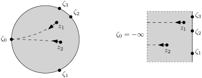
Figure 6.1. A summary of the conventions for $\mathring{\mathfrak{R}}_{d,m}$. The left picture follows (6.1.9), and the equivalent one on the right follows (6.1.10).

Remark 6.1.1.

Start with the space $\mathring{\mathfrak{M}}_{d+2m}$, and look at the involution which reverses the complex structure of the Riemann surface, and simultaneously acts on the set of marked points $(\zeta_{0},\dots,\zeta_{d},z_{1},\dots,z_{m},\bar{z}_{1},\dots,\bar{z}_{m})$ by exchanging $z_{k}$ and $\bar{z}_{k}$. That involution extends to $\mathfrak{M}_{d+2m}$, and we can lift it to the framed version. One can map $\mathfrak{R}_{d,m}$ to the fixed point set (real locus) of $\mathfrak{M}_{d+2m}^{\mathit{fr}}$, and derive its structure as manifold with corners from that.

6.1d. Punctured half-cylinders

Here we will look at a variation of the previous parameter space. For $d,m\geq 0$, consider punctured half-cylinders

(6.1.13) $$S=((-\infty,0]\times S^{1})\setminus\{z_{1},\dots,z_{m},\zeta_{0},\dots,\zeta_{d}\},$$

$$z_{1},\dots,z_{m}\in(-\infty,0)\times S^{1},\;\;\zeta_{0},\dots,\zeta_{d}\in\{0\}\times S^{1}\text{ in cyclic order}.$$

Denote the resulting parameter space by

(6.1.14) $$\mathring{\mathfrak{H}}_{d,m}=\mathit{Conf}_{m}((-\infty,0]\times S^{1})\times\mathit{Conf}_{d+1}^{\operatorname{ord}}(S^{1}).$$

Note that here, as in the previous (5.2.5), we are not dividing by rotations in $S^{1}$-direction. This space admits a compactification to a manifold with corners $\mathfrak{H}_{d,m}.$ As in the parallel situation of Section 5.2b, it is convenient to describe the compactification in two steps.

• We first introduce a space capturing bubbling in the interior of the cylinder, and disc bubbling at the boundary:

  (6.1.15) $$\mathfrak{H}_{d,m}^{\heartsuit}=\bigsqcup_{T}\mathring{\mathfrak{H}}_{T}^{\heartsuit},$$

  $$\mathring{\mathfrak{H}}_{T}^{\heartsuit}=\mathring{\mathfrak{H}}_{|v_{\operatorname{root}}|_{\operatorname{in}}^{\operatorname{op}},|v_{\operatorname{root}}|_{\operatorname{in}}^{\operatorname{cl}}}\times\prod_{\begin{subarray}{c}v\text{ open}\\ v\neq v_{\operatorname{root}}\end{subarray}}\mathring{\mathfrak{R}}_{|v|_{\operatorname{in}}^{\operatorname{op}},|v|_{\operatorname{in}}^{\operatorname{op}}}\times\prod_{v\text{ closed}}\mathring{\mathfrak{F}}_{|v|_{\operatorname{in}}}.$$

  Here, $T$ ranges over colored trees as before, but the stability condition at the root vertex has been dropped.

• The full compactification builds in breaking of the cylinder, as points go to $s=-\infty$. This can be formulated succinctly using the spaces from Section 5.2b:

  (6.1.16) $$\mathfrak{H}_{d,m}=\bigsqcup_{m_{1}+m_{2}=m,m_{1}>0}\mathfrak{C}_{m_{1}}\times\mathfrak{H}_{d,m_{2}}^{\heartsuit}.$$

The compactification is a manifold with corners. It carries an action of ${\mathbb{Z}}/(d+1){\mathbb{Z}}\times\mathit{Sym}(m)$ by permuting the punctures (cyclically for boundary punctures), and another application of Lemma 5.1.2 shows this action to be free.

The asymptotic markers at interior punctures, including $-\infty$, are chosen as in Section 5.2b. Correspondingly, the ends at interior punctures are as in (5.2.8), (5.2.9). At boundary punctures we pick them as in (6.1.6) but this time applied to $\zeta_{0}$ as well. This means that all boundary ends are considered as inputs, and parametrized by the positive half-cylinder $[0,\infty)\times[0,1]$. We can make a choice of those ends over the parameter spaces, which is compatible with gluing and also ${\mathbb{Z}}/(m+1){\mathbb{Z}}\times\mathit{Sym}(m)$-equivariant.

Remark 6.1.2.

The space $\mathfrak{H}_{d,m}$ carries a free $S^{1}$-action by rotating cylinders, and there is an isomorphism

(6.1.17) $$\mathfrak{H}_{d,m}/S^{1}\cong\mathfrak{R}_{d,m+1}.$$

In fact, if we take $\mathfrak{R}_{d,m+1}$ but label the interior punctures as $(z_{0},\dots,z_{m})$, then adding an arbitrary asymptotic marker at $z_{0}$ yields an $S^{1}$-bundle which is canonically isomorphic to $\mathfrak{H}_{d,m}$. Note however that this is incompatible with our choices of asymptotic markers at the other interior points: in the case of $\mathring{\mathfrak{H}}_{d,m}$ those markers point towards $z_{0}$, whereas for $\mathring{\mathfrak{R}}_{d,m+1}$ they point towards $\zeta_{0}$. For that reason, and in view of their differing applications, we have chosen different notation for those spaces.

6.1e. Angle-decorated half-cylinders

An angle-decorated half-cylinder is a surface (6.1.13) together with

(6.1.18) $$(\sigma_{1},\theta_{1}),\dots,(\sigma_{r},\theta_{r})\in(-\infty,0]\times S^{1},\;\;\sigma_{1}\leq\cdots\leq\sigma_{r}.$$

Let $\mathring{\mathfrak{AH}}_{d,m,r}$ be the resulting parameter space. Again, it admits a compacification to a manifold with corners $\mathfrak{AH}_{d,m,r}$. Note that breaking off of cylinders at $-\infty$ is subject to the same angle-twisting conventions as in Section 5.2c. On the codimension $1$ boundary face where two of the $\sigma_{i}$ collide, there is a forgetful map

(6.1.19) $$\partial_{\sigma_{i+1}=\sigma_{i}}\mathfrak{AH}_{d,m,r}\longrightarrow\mathfrak{AH}_{d,m,r-1}$$

which over $\mathring{\mathfrak{AH}}_{d,m,r}$ is defined as in (5.2.16). On the boundary face where the rightmost $\sigma_{r}$ becomes $0$, we have a map

(6.1.20) $$\partial_{\sigma_{r}=0}\mathfrak{AH}_{d,m,r}\longrightarrow\mathfrak{AH}_{d,m,r-1}$$

which over $\mathring{\mathfrak{AH}}_{d,m,r}$ is defined by forgetting $\sigma_{r}$ and then rotating the half-cylinder (with its punctures) by $-\theta_{r}$.

The asymptotic marker and end at $z_{0}=-\infty$ is chosen as in (5.2.18) (meaning, they are rotated by $\theta_{\operatorname{tot}}$), and the remaining ones follow the same idea as for the previously discussed half-cylinder spaces. When making a choice of ends over the parameter spaces, we always want them to be consistent with gluing; invariant under the (free) action of ${\mathbb{Z}}/(d+1){\mathbb{Z}}\times\mathit{Sym}(m)$; and compatible with both (6.1.19) and (6.1.20).

6.1f. Open-closed parameter spaces (1)

The open-closed map and its cyclic extension do not in fact use the entirety of the spaces $\mathring{\mathfrak{H}}_{d,m}$ and $\mathring{\mathfrak{AH}}_{d,m,r}$, but only certain subspaces. The first of these is the subset of those angle-decorated half-cylinders where

(6.1.21) $$\zeta_{0}=(0,0).$$

We denote it by $\mathring{\mathfrak{AH}}_{d,m,r}^{(1)}\subset\mathring{\mathfrak{AH}}_{d,m,r}$, and its closure by $\mathfrak{AH}_{d,m,r}^{(1)}\subset\mathfrak{AH}_{d,m,r}$. It is unproblematic to see that this is a submanifold with corners. For future reference, we list the codimension $1$ boundary strata (the first two already appear in $\mathring{\mathfrak{AH}}_{d,m,r}^{(1)}$, the others only in the compactification).

• One can have $\sigma_{i}=\sigma_{i+1}$ for some $0\leq i<r$, as in (6.1.19).

• One can have $\sigma_{r}=0$, as in (6.1.20).

• A cylinder can break off at $-\infty$, which yields an open stratum of the form

  (6.1.22) $$\mathring{\mathfrak{AC}}_{m_{1},r_{1}}\times\mathring{\mathfrak{AH}}_{d,m_{2},r_{2}}^{(1)},\;\;m_{1}+m_{2}=m,\;r_{1}+r_{2}=r.$$

• Several punctures (of either kind) converge towards a point on $\{0\}\times S^{1}$, and bubble off into a disc. These strata have the form

  (6.1.23) $$\mathring{\mathfrak{AH}}_{d_{1},m_{1},r_{1}}^{(1)}\times\mathring{\mathfrak{R}}_{d_{2},m_{2}},\;\;d_{1}+d_{2}=d+1,\;m_{1}+m_{2}=m.$$

• Fulton-Macpherson bubbling occurs at some interior point.

Remark 6.1.3.

Take the case $r=0$. The condition (6.1.21) and our standard choice of asymptotic markers combine to say that the asymptotic marker at the unique interior point $z_{0}=-\infty$ points towards $\zeta_{0}$. In terms of Remark 6.1.2, this means that

(6.1.24) $$\mathfrak{AH}_{d,m,0}^{(1)}\cong\mathfrak{R}_{d,m+1}.$$

If one then also sets $m=1$, the outcome is the space of discs with one interior puncture which appears in the classical construction of open-closed maps (e.g. [2]).

6.1g. Open-closed parameter spaces (2)

Our second space is again defined as a subset, or more precisely a codimension $0$ submanifold with boundary,

(6.1.25) $$\mathring{\mathfrak{AH}}_{d,m,r}^{(2)}\subset\mathring{\mathfrak{AH}}_{d-1,m,r}.$$

The jump in the value of $d$ accomodates the convention that specifically for $\mathring{\mathfrak{AH}}_{d,m,r}^{(2)}$, we number the boundary punctures by $\{\zeta_{1},\dots,\zeta_{d}\}$ (see Remark 6.1.6 below for motivation). With that in mind, the subset is defined by asking that

(6.1.26) $$(0,0)\text{ lies in the closed interval inside $\{0\}\times S^{1}$ which starts at $\zeta_{d}$ and ends at $\zeta_{1}$.}$$

Here, “starts and ends” is with respect to the natural boundary orientation, which is the same as that given by the ordering $\zeta_{1},\dots,\zeta_{d}$. (In the case $d=1$, the condition is empty, meaning that $\zeta_{1}$ may lie anywhere on $\{0\}\times S^{1}$; for $d=2$ it singles out one of the two closed intervals in $S^{1}$ with endpoints $\{\zeta_{1},\zeta_{2}\}$.) We define $\mathfrak{AH}_{d,m,r}^{(2)}$ to be the closure of $\mathring{\mathfrak{AH}}_{d,m,r}^{(2)}$ in $\mathfrak{AH}_{d-1,m,r}$. The codimension $1$ boundary faces are:

• counterparts of all five kinds previously encountered for type (1), which means the intersections of our space with the codimension $1$ boundary faces of $\mathfrak{AH}_{d-1,m,r}$;

• additionally, strata where $\zeta_{1}=(0,0)$ or $\zeta_{d}=(0,0)$.

The space $\mathfrak{AH}_{d,m,r}^{(2)}$ is not a manifold with corners. However, it is a manifold with boundary away from a set which is “of codimension $\geq 2$”, meaning that it is the union of pieces that are locally closed submanifolds of codimension $\geq 2$ in $\mathfrak{AH}_{d-1,m,r}$. This will be sufficient for our purpose, since all the data needed for Floer-theoretic constructions are first chosen over $\mathring{\mathfrak{AH}}_{d-1,m,r}$, in a way which is compatible with the compactification, and then restricted to (6.1.25). This applies in particular to the strip-like ends.

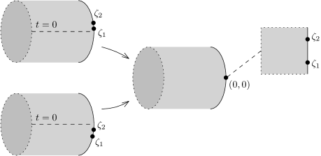
Figure 6.2. The limit $(\zeta_{1}^{\operatorname{lift}},\zeta_{2}^{\operatorname{lift}})\rightarrow(0,0)$ or $(1,1)$ in Example 6.1.4.

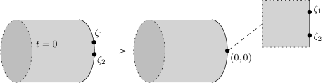
Figure 6.3. The limit $(\zeta_{1}^{\operatorname{lift}},\zeta_{2}^{\operatorname{lift}})\rightarrow(0,1)$ in Example 6.1.4.

Example 6.1.4.

Let’s look at the two-dimensional space

(6.1.27) $$\mathring{\mathfrak{AH}}_{2,0,0}^{(2)}\cong\{0\leq\zeta_{1}^{\operatorname{lift}}<\zeta_{2}^{\operatorname{lift}}\leq 1\}\setminus\{(0,1)\}.$$

where the position of the marked points has been lifted to $[0,1]$ by starting at $(0,0)$ and moving with the boundary operation. There are two boundary faces already visible in $\mathring{\mathfrak{AH}}_{2,0,0}$, namely $\zeta_{1}^{\operatorname{lift}}=0$ and $\zeta_{2}^{\operatorname{lift}}=1$. The limit where $\zeta_{1}^{\operatorname{lift}}=\zeta_{2}^{\operatorname{lift}}\in(0,1)$ is a standard bubbling process, giving rise to a smooth boundary side of the compactification. This takes care of the codimension $1$ faces.

The two corners $(0,0)$ and $(1,1)$ in the closure of (6.1.27) actually correspond to the same point in $\mathfrak{AH}_{2,0,0}^{(2)}$. The corresponding degeneration is shown in Figure 6.2. If one starts with the half-plane bubble with marked points at $(0,\pm 1)$, and glues the two parts together using small parameters $t\in{\mathbb{R}}$ (position of the attaching point) and $\gamma>0$ (gluing parameter) inherited from the larger space $\mathfrak{AH}_{1,0,0}$, the outcome (omitting some irrelevant constants) is a half-cylinder with $\zeta_{1}^{\operatorname{lift}}=t-\gamma$ and $\zeta_{2}^{\operatorname{lift}}=t+\gamma$. The condition (6.1.27) becomes

(6.1.28) $$t\leq-\gamma\text{ or }t\geq\gamma.$$

Hence, this is not even topologically a codimension $2$ corner. In contrast, the corner $(0,1)$ of (6.1.27) poses no complications, since there the analogue of (6.1.28) is $-\gamma\leq t\leq\gamma$ (Figure 6.3).

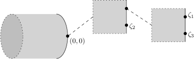
Figure 6.4. The point in $\mathfrak{AH}_{(3,0,0)}^{(2)}$ from Example 6.1.5.

Example 6.1.5.

A slightly more complicated case is

(6.1.29) $$\mathring{\mathfrak{AH}}_{3,0,0}^{(2)}\cong\{0\leq\zeta_{1}^{\operatorname{lift}}<\zeta_{2}^{\operatorname{lift}}<\zeta_{3}^{\operatorname{lift}}\leq 1\}\setminus(\{0\}\times(0,1)\times\{1\}).$$

Instead of discussing the entire compactification, we’ll just focus on the neighbourhood of a single point, shown in Figure 6.4. In the larger space $\mathfrak{AH}_{2,0,0}$, a neighbourhood of this point is parametrized by $t\in{\mathbb{R}}$ (position of the attaching point on the boundary of the half-cylinder) and $\gamma_{1},\gamma_{2}\geq 0$ (gluing parameters). Assuming the marked points on both half-planes start out at $(0,\pm 1)$, gluing roughly yields

(6.1.30) $$\zeta_{1}=(0,\gamma_{1}\gamma_{2}+t),\;\zeta_{2}=(-\gamma_{1}+t),\;\zeta_{3}=(0,-\gamma_{1}\gamma_{2}+t).$$

For this to lie in (6.1.29) one needs $-\gamma_{1}\gamma_{2}\leq t\leq\gamma_{1}\gamma_{2}$; which is not a corner in the $C^{\infty}$-sense, since the graphs of $\pm\gamma_{1}\gamma_{2}$ become tangent at $(\gamma_{1},\gamma_{2})=(0,0)$.

Remark 6.1.6.

It can make sense to consider the half-cylinder as coming with an additional decoration $\zeta_{0}^{+}=(0,0)$, which can agree with either $\zeta_{d}$ or $\zeta_{1}$, and otherwise has to be such that $(\zeta_{0}^{+},\zeta_{1},\dots,\zeta_{d})$ appear in cyclic order. This makes the situation more parallel to (6.1.21). In particular, the choice of asymptotic marker in both cases is rotated by $\theta_{\operatorname{tot}}$ from the direction pointing towards $\zeta_{0}$ respectively $\zeta_{0}^{+}$. It is also intuitive in view of the definition of the cyclic complex (3.2.25), where $\zeta_{0}^{+}$ can be thought of as standing in for the artificial unit $e^{+}$. Note that such a $\zeta_{0}^{+}$ would merely be a mnemonic for remembering (6.1.26), and not a marked point or puncture, hence cannot bubble off. This is where our approach differs from that in [32, Section 5.2]: there, $\zeta_{0}^{+}$ (written as $z_{f}$) is treated as a marked point, leading to a larger compactification which is geometrically better-behaved but has additional codimension $1$ boundary strata [32, Remark 45]. For instance, take the situation from Example 6.1.4. If one treats $\zeta_{0}^{+}$ as a puncture, the resulting compactification is isomorphic to $\mathfrak{R}_{1,2}$, which is a hexagon. In comparison with our compactification, not only have the limit points $(0,0)$ and $(1,1)$ in (6.1.27) now become separate, each of them has actually been expanded into an entire boundary interval, and the same expansion has happened to $(0,1)$.

6.2. Open-string operations

6.2a. The Fukaya category

We recall briefly the construction of the wrapped Fukaya category of $(\hat{N},\theta_{\hat{N}})$ using quadratic Hamiltonians, as in [2]. Fix a finite collection of Lagrangian submanifolds, which are conical (4.2.7), carry brane structures (4.2.16), and such that each pair $(L_{0},L_{1})$ satisfies Assumption 4.2.3 (with a fixed $P$, the same for all pairs). These will be the objects of our category. For every pair of objects we choose Floer data $(H_{L_{0},L_{1}},J_{L_{0},L_{1}})$ as in Section 4.2c; suppressing the choices from the notation, we write $(\mathit{CF}^{*}(L_{0},L_{1}),\delta)$ for the resulting the Floer complex.

For each $d\geq 2$, we fix a consistent choice of strip-like ends $\varepsilon_{0},\varepsilon_{1},\cdots,\varepsilon_{d}$ over $\mathring{\mathfrak{R}_{d}}$ (Section 6.1a). On the universal families $U_{\mathfrak{R}_{d}}\longrightarrow\mathfrak{R}_{d}$, we choose perturbation data

(6.2.1) $$K_{\mathfrak{R}_{d}}\in\Omega^{1}_{\mathcal{U}_{\mathfrak{R}_{d}}/\mathfrak{R}_{d}}(U_{\mathfrak{R}_{d}},\mathcal{H}(\hat{N}))\text{ and }J_{\mathfrak{R}_{d}}\in C^{\infty}(U_{\mathfrak{R}_{d}},\mathcal{J}(\hat{N})).$$

These should satisfy the conditions of Section 4.2d when restricted to each fiber of the universal curve, and should be conformally consistent with respect to boundary strata (this is the open string analogue of the condition from Section 4.1h). Take chords $\mathbf{y}=(y_{0},y_{1},\cdots,y_{d})$, where $y_{0}$ is associated to the pair $(L_{0},L_{d})$, and each $y_{i}$, $i>0$, is associated to $(L_{i-1},L_{i})$. We then consider the parametrized moduli space $\mathring{\mathfrak{R}}_{d}(\mathbf{y})$ of pairs $(r,u)$, where $r\in\mathring{\mathfrak{R}}_{d}$ and $u:S_{r}\rightarrow M$ is a solution to (4.1.6), (4.2.3), (4.2.19). For a generic choice of perturbation data, these moduli spaces are smooth manifolds with

(6.2.2) $$\mathrm{dim}\,\mathring{\mathfrak{R}}_{d}(\mathbf{y})=\operatorname{deg}(y_{0})-\sum_{i}\operatorname{deg}(y_{i})+d-2.$$

Moreover, they admit Gromov compactifications $\mathfrak{R}_{d}(\mathbf{y})$, and in particular are finite sets if the dimension is $0$. As in the corresponding closed string context of Section 4.1g, an isolated point $(r,u)$ gives rise to an isomorphism $o(r,u):\mathfrak{o}_{y_{1}}\otimes\cdots\otimes\mathfrak{o}_{y_{m}}\cong\mathfrak{o}_{y_{0}}$. The ${\mathbb{K}}$-normalizations of those isomorphisms yield the $A_{\infty}$-operations

(6.2.3) $$\mu^{d}:\mathit{CF}^{*}(L_{0},L_{1})\otimes\cdots\otimes\mathit{CF}^{*}(L_{d-1},L_{d})\longrightarrow\mathit{CF}^{*+2-d}(L_{0},L_{d})$$

for $d\geq 2$; for $d=1$ we use the Floer differential.

6.2b. The deformed Fukaya category

This section explains how to deform the Fukaya category using a Maurer-Cartan element (5.3.25). The objects will be the same as before. The structure maps

(6.2.4) $$\mu_{q}^{d}:\mathit{CF}^{*}(L_{0},L_{1})\otimes\cdots\otimes\mathit{CF}^{*}(L_{d-1},L_{d})\to\mathit{CF}^{*}(L_{0},L_{d})[[q]]$$

reduce to the previous ones for $q=0$ (which in particular means that $\mu^{0}_{q}$ has zero $q$-constant term). To define the $q$-deformed operations, we use the parameter spaces $\mathring{\mathfrak{R}_{d,m}}$. We assume that ends have been chosen for those spaces, as in Section 6.1c, and we also choose perturbation data for the universal families over them, generalizing (6.2.1). Since the action of $\mathit{Sym}(m)$ on $\mathfrak{R}_{d,m}$ is free, we can achieve transversality while simultaneously asking that the perturbation data be $\mathit{Sym}(m)$-equivariant.

Having made these choices, given a collection of chords $\mathbf{y}=(y_{0},y_{1},\cdots,y_{d})$ and periodic orbits $\mathbf{x}=(x_{1},\cdots,x_{m})$, the resulting parametrized moduli spaces $\mathring{\mathfrak{R}}_{d,m}(\mathbf{y},\mathbf{x})$ satisfy

(6.2.5) $$\operatorname{dim}\,\mathring{\mathfrak{R}}_{d,m}(\mathbf{y},\mathbf{x})=\operatorname{deg}(y_{0})-\sum_{i=1}^{d}\operatorname{deg}(y_{i})-\sum_{j=1}^{m}\operatorname{deg}(x_{j})+d-2+2m.$$

Counting isolated solutions gives rise to operations

(6.2.6) $$\mu^{d,m}:\mathit{CF}^{*}(L_{0},L_{1})\otimes\cdots\otimes\mathit{CF}^{*}(L_{d-1},L_{d})\otimes\mathit{CF}^{*}(H)^{\otimes m}\longrightarrow\mathit{CF}^{*+2-d-2m}(L_{0},L_{d}).$$

We include the previously defined $A_{\infty}$-structure here as the special case $m=0$. Then, (6.2.4) is defined by inserting the Maurer-Cartan element $\alpha$ in the way familiar from the closed string constructions in Section 5.3e:

(6.2.7) $$\mu_{q}^{d}(y_{1},\cdots,y_{d})\stackrel{{\scriptstyle\mathrm{def}}}{{=}}\sum_{m\geq 0}{\textstyle\frac{1}{m!}}\,\mu^{d,m}(y_{1},\cdots,y_{d},\alpha^{\otimes m})\in\mathit{CF}^{*}(L_{0},L_{d})[[q]].$$

Proposition 6.2.1.

The operations (6.2.4) define a curved $A_{\infty}$-deformation $\mathcal{A}_{q}$ of $\mathcal{A}$.

Proof.

The proof again proceeds by examining the boundaries of one-dimensional moduli spaces $\mathfrak{R}_{d,m}(\mathbf{y},\mathbf{x}))$. There are four different kinds of boundary points:

• Floer cylinder breaking at one of the interior marked points.

• Degeneration of the domain to the codimension one strata where $2\leq m_{1}\leq m$ of the interior marked points collide. On the parameter space $\mathfrak{R}_{d,m}$, this means that we converge to a point in a stratum

  (6.2.8) $$\mathring{\mathfrak{R}}_{d,m_{2}}\times\mathring{\mathfrak{F}}_{m_{1}}\subset\partial\mathfrak{R}_{d,m},\;\;m_{1}+m_{2}=m+1.$$

• Floer strip breaking at a boundary marked point.

• Boundary marked points collide, or interior marked points approach the boundary (or both). On the parameter space, this means convergence to a point in

  (6.2.9) $$\mathring{\mathfrak{R}}_{d_{2},m_{2}}\times\mathring{\mathfrak{R}}_{d_{1},m_{1}}\subset\partial\mathfrak{R}_{d,m},\;\;m_{1}+m_{2}=m,\;d_{1}+d_{2}=d+1.$$

The fact that $\alpha$ satisfies the Maurer-Cartan equation means that the sum of the first two contributions is zero. The third and fourth kind of degeneration account for the terms in the $A_{\infty}$-equation. ∎

6.2c. The deformed closed-open map

The same moduli spaces as in the definition of $\mathcal{A}_{q}$ also give rise to a deformation of the closed-open string map. Given $w\in\mathit{CF}_{q}^{\operatorname{diag}}(H)$ (see (5.3.26) for the notation), we insert $\alpha$ into the first $(m-1)$ closed string entries, and $w$ into the $m$-th entry, of the operation $\mu^{d,m}$ from (6.2.6); and write the outcome as

(6.2.10) $$\mathit{CO}_{q}^{d}:\mathit{CF}_{q}^{\operatorname{diag}}(H)\longrightarrow\mathit{hom}(\mathcal{A}(L_{0},L_{1},\dots,L_{d}),\mathcal{A}(L_{0},L_{d}))[[q]],$$

$$CO_{q}^{d}(w)=\sum_{m\geq 1}\textstyle{\frac{1}{(m-1)!}}\,\mu^{d,m}(\dots,\alpha^{\otimes m-1},w).$$

The collection of all such maps, for $d\geq 0$, yields

(6.2.11) $$\mathit{CO}_{q}:\mathit{CF}_{q}^{\operatorname{diag}}(H)\longrightarrow C^{*}(\mathcal{A}_{q}).$$

A variant of Proposition 6.2.1 shows that this is a chain map; compared to the argument given there, the new boundary points of one-dimensional moduli spaces happens when a Floer cylinder of Fulton-MacPherson configuration which contains the point $z_{m}$ bubbles off. The contribution from those boundary points is precisely $\mathit{CO}_{q}\circ\delta_{q}^{\operatorname{diag}}$, which is part of the chain map equation.

6.2d. The deformed cyclic open-closed map

In this section, we construct the deformed cyclic open-closed map

(6.2.12) $$\mathit{OC}_{S^{1},q}:\mathit{CC}_{*}^{+}(\mathcal{A}_{q})\longrightarrow CF_{S^{1},q}^{*+n}(H).$$

After setting $q=0$ (or, geometrically, eliminating the extra interior punctures), this reduces to the construction from [32]. In view of the definition of $\mathit{CC}_{*}^{+}(\mathcal{A}_{q})$, see (3.2.36), the map (6.2.12) has components

(6.2.13) $$\mathit{OC}_{S^{1},q,(1)}:\mathcal{A}_{q}(L_{d},L_{0},L_{1},\dots,L_{d})\longrightarrow\mathit{CF}_{S^{1},q}^{*+n-d}(H),$$

(6.2.14) $$\mathit{OC}_{S^{1},q,(2)}:e_{\mathcal{A}}^{+}\otimes\mathcal{A}(L_{0},L_{1},\dots,L_{d-1},L_{0})\longrightarrow\mathit{CF}_{S^{1},q}^{*+n-d}(H).$$

In addition to those, we will introduce another operation $\mathit{AH}_{S^{1},q,(0)}$ which plays a purely expository role (since it can ultimately be written in terms of $\mathit{OC}_{S^{1},q,(2)}$).

To set up the construction, we choose perturbation data over the moduli spaces of angle-decorated half-cylinders $\mathfrak{AH}_{d,m,r}$. These must lie in the class of perturbations allowed in Section 4.2e, and should be invariant with respect to ${\mathbb{Z}}/(d+1){\mathbb{Z}}\times\mathit{Sym}(m)$ (which acts freely on the parameter space, see the discussion in Section 6.1e). In addition to the usual conformal consistency conditions with respect to degenerations of the surfaces, we require that along certain boundary strata, the Floer data are pulled back from lower-dimensional parameter spaces:

• over $\partial_{\sigma_{i+1}=\sigma_{i}}\mathring{\mathfrak{AH}}_{d,m,r}$, the perturbation data are pulled back along (6.1.19).

• Along $\partial_{\sigma_{r}=0}\mathring{\mathfrak{AH}}_{d,m,r}$, the perturbation data are pulled back along (6.1.20).

Further conditions will be added throughout the subsequent discussion (one imposes them as part of the initial choice, but from an expository viewpoint it makes more sense to discuss them at the point where they are needed).

Let’s first consider the moduli spaces $\mathring{\mathfrak{AH}}_{d,m,r}(\mathbf{y},\mathbf{x})$ parametrized over $\mathring{\mathfrak{AH}}_{d,m,r}$. Here, $\mathbf{x}=(x_{0},x_{1},\cdots,x_{m})$ are periodic orbits, where $x_{0}$ is placed at the output $s=-\infty$, and $\mathbf{y}=(y_{0},\dots,y_{d})$ are chords. The zero-dimensional spaces give rise to operations

(6.2.15) $$\mathit{AH}^{d,m,r}:\mathcal{A}(L_{d},L_{0},L_{1},\dots,L_{d})\otimes\mathit{CF}^{*}(H)^{\otimes m}\longrightarrow\mathit{CF}^{*+n-d-2r-2m-1}(H).$$

We insert $\alpha$ at the $m$ closed string inputs, add up over all $m$, and also and add up over all $r$ with powers $u^{r}$; the outcome being maps

(6.2.16) $$\mathit{AH}_{S^{1},q}:\mathcal{A}_{q}(X_{d},X_{0},\dots,X_{d})\longrightarrow\mathit{CF}^{*+n-d-1}_{S^{1},q}(H).$$

Next take the subspace $\mathring{\mathfrak{AH}}_{d,m,r}^{(1)}$ from Section 6.1f. The perturbation data that we use on these moduli spaces will be pulled back from $\mathring{\mathfrak{AH}}_{d,m,r}$, with the following condition on the original choice:

• the parametrized moduli spaces $\mathring{\mathfrak{AH}}_{d,m,r}^{(1)}(\mathbf{y},\mathbf{x})$ are regular; or equivalently, the map $\mathring{\mathfrak{AH}}_{d,m,r}(\mathbf{y},\mathbf{x})\rightarrow\mathring{\mathfrak{AH}}_{d,m,r}$ is transverse to the submanifold $\mathring{\mathfrak{AH}}_{d,m,r}^{(1)}$.

The zero-dimensional moduli spaces spaces define operations

(6.2.17) $$\mathit{OC}^{d,m,r}_{(1)}:\mathcal{A}(L_{d},L_{0},L_{1},\dots,L_{d})\otimes\mathit{CF}^{*}(H)^{\otimes m}\longrightarrow\mathit{CF}^{*+n-d-2r-2m}(H),$$

which we manipulate algebraically as before to get (6.2.13).

As in our discussion of parameter spaces in Section 6.1g, we will now change conventions slightly: the number of boundary punctures is written as $d>0$, and they will be numbered by $\{\zeta_{1},\dots,\zeta_{d}\}$. The Lagrangian submanifolds involved are correspondingly $(L_{0},\dots,L_{d-1})$. We use the subspace $\mathring{\mathfrak{AH}}_{d,m,r}^{(2)}\subset\mathring{\mathfrak{AH}}_{d-1,m,r}$ and the associated parametrized moduli spaces $\mathring{\mathfrak{AH}}_{d,m,r}^{(2)}(\mathbf{y},\mathbf{x})$. The additional transversality requirement is:

• The moduli spaces $\mathfrak{AH}_{d,m,r}^{(2)}(\mathbf{y},\mathbf{x})$ of (expected) dimension $\leq 1$ contain no curves lying over the codimension two or higher boundary strata of $\mathfrak{AH}_{d,m,r}^{(2)}$.

Using those spaces, we define maps

(6.2.18) $$\mathit{OC}^{d,m,r}_{(2)}:e^{+}_{\mathcal{A}}\otimes\mathcal{A}(L_{0},L_{1},\dots,L_{d},L_{0})\otimes\mathit{CF}^{*}(H)^{\otimes m}\longrightarrow\mathit{CF}^{*+n-d-2r-2m}(H),$$

which then lead to (6.2.14).

Take the Connes operator which is part of (3.2.26), =

(6.2.19) $$B(a_{0}(a_{1}|\dots|a_{d}))=-\sum_{j}(-1)^{(\|a_{0}\|+\cdots+\|a_{j}\|)(\|a_{j+1}\|+\cdots+\|a_{d}|)}e_{\mathcal{A}}^{+}(a_{j+1}|\dots|a_{d}|a_{0}|\dots|a_{j}).$$

Lemma 6.2.2.

The operations (6.2.16) and (6.2.14) are related by

(6.2.20) $$\mathit{AH}_{S^{1},q}(a_{0}(a_{1}|\dots|a_{d}))=OC_{S^{1},q,(2)}\circ B(a_{0}(a_{1}|\dots|a_{d})).$$

Sketch of proof.

In the moduli spaces $\mathring{\mathfrak{AH}}_{d,m,r}(\mathbf{y},\mathbf{x})$, the point $(0,0)$ can lie between any two consecutive boundary marked points. (The situation where $(0,0)$ agrees with one of the marked points $\zeta_{j}$ is codimension $1$ and can be ignored.) Suppose $(0,0)$ lies between $\zeta_{j}$ and $\zeta_{j+1}$. Because the Floer data have been chosen equivariantly under cyclic permutation of the boundary marked points, we can view this as contributing to $\pm OC_{S^{1},q,(2)}\circ e_{\mathcal{A}}^{+}(a_{j+1}|\dots|a_{d}|a_{0}|\dots|a_{j}).$ The boundary of the disc is naturally decomposed into intervals lying between consecutive marked points, and so summing over all $j$ proves (6.2.20). ∎

Proposition 6.2.3.

The following equation holds:

(6.2.21) $$\mathit{OC}_{S^{1},q,(1)}\circ d_{\mathit{C}_{*}^{+}(\mathcal{A}_{q})}(a_{0}(a_{1}|\dots|a_{d}))+u\mathit{OC}_{S^{1},q,(2)}\circ B(a_{0}(a_{1}|\dots|a_{d}))$$

$$=\delta_{S^{1},q}\circ\mathit{OC}_{S^{1},q,(1)}(a_{0}(a_{1}|\dots|a_{d})).$$

Proof.

The contributions from codimension one boundary strata of $\mathring{\mathfrak{AH}}_{d,m,r}^{(1)}(\mathbf{y},\mathbf{x})$ are as follows:

• We have the boundary strata where $\sigma_{i+1}=\sigma_{i}$. These do not contribute because the Floer data is pulled back from a lower-dimensional space along (6.1.19).

• We can have Floer breaking or Fulton-MacPherson bubbling at some interior point. As in prior situations, the Maurer-Cartan equation ensures this contributes nothing.

• Consider the stratum where $\sigma_{r}=0$. Away from higher codimension subsets, the map (6.1.20) defines an isomorphism from this boundary stratum to $\mathring{\mathfrak{AH}}_{d,m,r-1}$. As the Floer data is pulled back from there, the argument from Lemma 6.2.2 shows that this stratum contributes the term $u\mathit{OC}_{S^{1},q,(2)}\circ B(a_{0}(a_{1}|\dots|a_{d}))$.

• We can have Floer cylindrical breaking or degeneration as $s\to-\infty$, which yields the term $\delta_{S^{1},q}\circ OC_{S^{1},q,(1)}$.

• Floer strip breaking or disc bubbling at the boundary contributes the term $OC_{S^{1},q,(1)}\circ d_{\mathit{C}_{*}^{+}(\mathcal{A}_{q})}(a_{0}(a_{1}|\dots|a_{d}))$.

∎

Proposition 6.2.4.

The following equation is also satisfied:

(6.2.22) $$-\mathit{OC}_{S^{1},q,(2)}\circ e^{+}_{\mathcal{A}}\,d_{D_{*}(\mathcal{A}_{q})}(a_{1}|\dots|a_{d}))+\mathit{OC}_{S^{1},q,(1)}(a_{1}(a_{2}|\dots|a_{d}))$$

$$\qquad-(-1)^{\|a_{d}\|(\|a_{1}\|+\cdots+\|a_{d-1}\|)}\mathit{OC}_{S^{1},q,(1)}(a_{d}(a_{1}|\dots|a_{d-1}))$$

$$=\delta_{S^{1},q}\circ OC_{S^{1},q,(2)}(e_{\mathcal{A}}^{+}(a_{1}|\dots|a_{d})).$$

Proof.

Consider the contributions from codimension one boundary points of $\mathring{\mathfrak{AH}}_{d,m,r}^{(2)}(\mathbf{y},\mathbf{x})$:

• As usual, the boundary strata where $\sigma_{i+1}=\sigma_{i}$ contribute nothing, because the Floer data are pulled back from a lower-dimensional space.

• We can have Floer breaking or Fulton-MacPherson bubbling at some interior point. Again, the Maurer-Cartan equation ensures this contributes nothing.

• This time, the stratum where $\sigma_{r}=0$ also contributes nothing because the perturbation data is pulled back from $\mathring{\mathfrak{AH}}_{d-1,m,r-1}$, which is a lower-dimensional parameter space, along (6.1.20).

• As in the previous Proposition, we can have a cylinder breaking off at $s\to-\infty$, which now yields the term $\delta_{S^{1},q}\circ OC_{S^{1},q,(2)}$.

• Floer strip breaking or disc bubbling at the boundary gives rise to $e^{+}_{\mathcal{A}}\,d_{D_{*}(\mathcal{A}_{q})}(a_{1}|\dots|a_{d})$.

• The remaining boundary strata are where $\zeta_{1}=(0,0)$ or $\zeta_{d}=(0,0)$. These boundaries contribute the last two terms on the left hand side of (6.2.22).

∎

The two Propositions above combine to show that $\mathit{OC}_{S^{1},q}$ is a chain map.

6.3. The cyclic open-closed map and connections

6.3a. The modified Getzler-Gauss-Manin connection

Start with the operations $\mu^{d,m}$ from (6.2.6) and $\mu^{d}_{q}$ from (6.2.7) and consider

(6.3.1) $$\partial_{q}\mu^{d}_{q}:\mathcal{A}_{q}(L_{0},L_{1},\dots,L_{d})\longrightarrow\mathcal{A}_{q}(L_{0},L_{d})[-d],$$

$$(\partial_{q}\mu^{d}_{q})(a_{1},\dots,a_{d})=\sum_{m\geq 1}\textstyle{\frac{1}{(m-1)!}}\mu^{d,m}(a_{1},\dots,a_{d},\partial_{q}\alpha,\alpha^{\otimes m-1}).$$

In constructing additional operations, we will always proceed as follows:

• Geometrically, we will use subsets of the space $\mathring{\mathfrak{R}}_{d,m}$ (where we always have $m>0$) of discs with boundary and interior punctures (Section 6.1c). We also recycle the choices of ends and of additional data used in the definition of the deformed Fukaya category (Section 6.2b), which means that the compactifications of the moduli spaces of pseudo-holomorphic maps are inherited from there. An additional transversality condition will be imposed on those data, but that can be achieved as part of the initial generic choice.

• Algebraically, the resulting operations will always be defined in the same fashion as the right hand side of (6.3.1), which means: inserting $\partial_{q}\alpha$ at $z_{1}$, and $\alpha$ at all other interior punctures; and then summing with weight $\frac{1}{(m-1)!}$, which one can think of as accounting for permutations of $(z_{2},\dots,z_{m})$.

Let’s split $\mathring{\mathfrak{R}}_{d,m}$ into halves, based on the position of $z_{1}$. Say that our discs $S$ have $j+k+2$ boundary punctures, for some $j,k\geq 0$ ($d=j+k+1\geq 1$). We fix $\bar{S}\cong{\mathbb{D}}$ so that

(6.3.2) $$\zeta_{0}=-1,\,\zeta_{j+1}=1\in\partial{\mathbb{D}}.$$

With this convention, define $\mathring{\mathfrak{R}}^{\pm}_{j,1,k,m}\subset\mathring{\mathfrak{R}}_{j+k+1,m}$ by requiring that (Figure 6.5)

(6.3.3) $$\pm\!\mathrm{im}(z_{1})\geq 0.$$

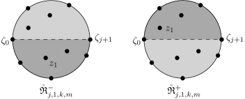
Figure 6.5. The position constraint from (6.3.3) which defines $\mathring{\mathfrak{R}}^{\pm}_{j,1,k,m}$ (as shown, $j=3$, $k=2$, $m=4$).

Let’s start by looking at the common boundary

(6.3.4) $$\mathring{\mathfrak{R}}^{0}_{j,1,k,m}=\partial\mathring{\mathfrak{R}}^{+}_{j,1,k,m}=\partial\mathring{\mathfrak{R}}^{-}_{j,1,k,m}=\{\mathrm{im}(z_{1})=0\}$$

(on that boundary, one could break the remaining symmetry by requiring that $z_{1}=0\in{\mathbb{D}}$). The additional transversality condition mentioned at the start of the discussion is precisely that the moduli space of pseudo-holomorphic maps parametrized by $\mathring{\mathfrak{R}}_{j,1,k,m}^{0}$ should be regular (equivalently, if we take all of $\mathring{\mathfrak{R}}_{d,m}$ as a parameter space, then the projection from the space of maps to the parameter space should be transverse to $\mathring{\mathfrak{R}}^{0}_{j,1,k,m}$ for each of the finitely many $(j,k)$ that can occur). The operations obtained from the space of pseudo-holomorphic maps parametrized by $\mathring{\mathfrak{R}}^{0}_{j,1,k,m}$, which we call

(6.3.5) $$\mathit{GM}^{j,1,k}_{0}:\mathcal{A}_{q}(L_{0},L_{1},\dots,L_{j+k+1})\longrightarrow\mathcal{A}_{q}(L_{0},L_{j+k+1})[-j-k],$$

form an $\mathcal{A}_{q}$-bimodule homomorphism (from the diagonal to itself). In the list of codimension $1$ degenerations from Figure 6.6, the top four are terms in the bimodule map equation; and the bottom two contribute zero (the first by the Maurer-Cartan equation, the second by (3.4.12); this is another argument we’ve seen before, in Section 5.3f).

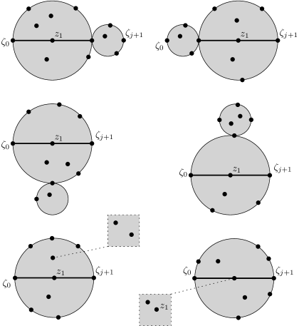
Figure 6.6. Codimension $1$ degenerations for $\mathfrak{R}_{j,1,k,m}^{0}$.

If we now pass to the spaces $\mathring{\mathfrak{R}}^{\pm}_{j,1,k,m}$ themselves, the same kinds of degenerations as before appear; and there is an additional degeneration, where $z_{1}$ approaches the lower (for $\mathfrak{R}^{-}$) or upper (for $\mathfrak{R}^{+}$) half of $\partial{\mathbb{D}}$. Finally, the parameter space itself has boundary (6.3.4), and that also contributes to the boundaries of one-dimensional moduli spaces. The outcome is the associated operations

(6.3.6) $$\mathit{GM}^{j,1,k}_{\pm}:\mathcal{A}_{q}(L_{0},L_{1},\dots,L_{j+k+1})\longrightarrow\mathcal{A}_{q}(L_{0},L_{j+k+1})[-j-k-1],$$

$$\mathit{GM}_{-}^{j,1,k}+\mathit{GM}_{+}^{j,1,k}=\partial_{q}\mu_{\mathcal{A}_{q}}^{j+k+1},$$

satisfy the following equations, with respect to the differential $d_{(\mathcal{A}_{q},\mathcal{A}_{q})}$ in the dg category of $\mathcal{A}_{q}$-bimodules:

(6.3.7) $$\begin{aligned} &(d_{(\mathcal{A}_{q},\mathcal{A}_{q})}\mathit{GM}_{-})^{j,1,k}(a_{1},\dots,\underline{a_{j+1}},\dots,a_{j+k+1})=\mathit{GM}_{0}^{j,1,k}(a_{1},\dots,a_{j+k+1})\\ &\quad-\sum_{il}\pm\mu_{\mathcal{A}_{q}}^{j+k-l+2}(a_{1},\dots,a_{i},\partial_{q}\mu_{\mathcal{A}_{q}}^{l}(a_{i+1},\dots,a_{i+l}),\dots,\underline{a_{j+1}},\dots,a_{j+k+1}),\end{aligned}$$

(6.3.8) $$\begin{aligned} &(d_{(\mathcal{A}_{q},\mathcal{A}_{q})}\mathit{GM}_{+})^{j,1,k}(a_{1},\dots,\underline{a_{j+1}},\dots,a_{j+k+1})=-\mathit{GM}_{0}^{j,1,k}(a_{1},\dots,a_{j+k+1})\\ \ &\quad+\sum_{il}\pm\mu_{\mathcal{A}_{q}}^{j+k-l+2}(a_{1},\dots,\underline{a_{j+1}},\dots\partial_{q}\mu_{\mathcal{A}_{q}}^{l}(a_{i+1},\dots,a_{i+l}),\dots,a_{j+k+1}).\end{aligned}$$

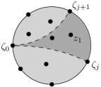
Figure 6.7. The position constraint from (6.3.9), which defines $\mathring{\mathfrak{R}}_{j,h,m}^{\prec}$ (as shown here, $j=3$, $h=2$, $m=5$).

We use $\mathit{GM}=\mathit{GM}_{-}$ to modify the Getzler-Gauss-Manin connection, in the general algebraic way indicated in (3.2.31)–(3.2.33). The last-mentioned equation can be given a more geometric meaning, as follows. In (6.3.2) we could work with $\zeta_{0}$, $\zeta_{j+1}$ in arbitrary position, dividing by the entire automorphism group of the disc; then the role of the line $\{\mathrm{im}(z)=0\}$ would be played by the hyperbolic geodesic connecting those two boundary points. In that perspective, the first term in (3.2.33) concerns surfaces where $z_{1}$ lies in a region bounded by the geodesic connecting $\zeta_{0}$ to $\zeta_{j+1}$, whereas the second term is the same for the region connecting $\zeta_{0}$ to $\zeta_{j}$. Subtracting those two contributions from each other leads us to consider surfaces with the following modified condition:

(6.3.9) $$z_{1} S \zeta_{0} \zeta_{j} \zeta_{0} \zeta_{j+1} \partial S \zeta_{j} \zeta_{j+1}$$ lies in the closed region of bounded by: the hyperbolic geodesic connecting to ; the hyperbolic geodesic connecting to ; and the part of between and (Figure 6.7).

Write $\mathring{\mathfrak{R}}_{j,h,m}^{\prec}$ for the space of such surfaces, where $h=d-j$. Following our usual principle, this gives rise to operations

(6.3.10) $$\mathit{GM}_{\prec}^{j,h}:\mathcal{A}_{q}(L_{0},L_{1},\dots,L_{j+h})\longrightarrow\mathcal{A}_{q}(L_{0},L_{j+h})[-j-h],$$

$$\mathit{GM}_{\prec}^{j,h}=\mathit{GM}_{-}^{j,1,h-1}-\mathit{GM}_{-}^{j-1,1,h}.$$

As given, the definition only makes sense when $j,h>0$, but we extend it by setting (Figure 6.8)

(6.3.11) $$\mathring{\mathfrak{R}}^{\prec}_{0,h,m}=\mathring{\mathfrak{R}}_{0,1,h-1,m}^{-}\;\;\Longrightarrow\;\;\mathit{GM}_{\prec}^{0,h}=\mathit{GM}_{-}^{0,1,h-1}\text{ for $h>0$},$$

$$\mathring{\mathfrak{R}}^{\prec}_{j,0,m}=\mathring{\mathfrak{R}}_{j-1,1,0,m}^{+}\;\;\Longrightarrow\;\;\mathit{GM}_{\prec}^{j,0}=\mathit{GM}_{+}^{j-1,1,0}\text{ for $j>0$},$$

$$\mathring{\mathfrak{R}}^{\prec}_{0,0,m}=\mathring{\mathfrak{R}}_{0,m}\;\;\Longrightarrow\mathit{GM}_{\prec}^{0,0}=\partial_{q}\mu_{\mathcal{A}_{q}}^{0}.$$

Combining this with the relation between $\mathit{GM}_{\pm}$ from (6.3.6), the modified connection is:

(6.3.12) $$\tilde{\nabla}_{u\partial_{q}}(a_{0}(a_{1}|\dots|a_{l}))=u(\partial_{q}a_{0})(a_{1}|\dots|a_{l})+u\sum_{i}a_{0}(a_{1}|\dots|\partial_{q}a_{i}|\dots|a_{l})$$

$$\qquad+\sum_{jk}\pm\mathit{GM}_{0}^{j,1,k}(a_{l-j+1},\dots,\underline{a_{0}},\dots,a_{k})(a_{k+1}|\dots|a_{l-j})$$

$$\qquad+u\sum_{ijk}\pm e_{\mathcal{A}}^{+}(a_{i+1}|\dots|\partial_{q}\mu_{\mathcal{A}_{q}}^{k}(a_{j+1},\dots,a_{j+k})|\dots|a_{0}|\dots|a_{i})$$

$$\qquad+u\sum_{ijk}\pm e^{+}_{\mathcal{A}}(a_{i+1}|\dots|\mathit{GM}_{-}^{l-j,1,k}(a_{j+1},\dots,a_{l},\underline{a_{0}},a_{1},\dots,a_{k})|\dots|a_{i})$$

$$\qquad\qquad\qquad\qquad\qquad\text{for }a_{0}(a_{1}|\dots|a_{l})\in C_{*}(\mathcal{A}_{q})[[u]],$$

$$\tilde{\nabla}_{u\partial_{q}}(e_{\mathcal{A}}^{+}(a_{1}|\dots|a_{l}))=u\sum_{i}e_{\mathcal{A}}^{+}(a_{1}|\dots|\partial_{q}a_{i}|\dots|a_{l})$$

$$\qquad+\sum_{jh}\pm\mathit{GM}_{\prec}^{j,h}(a_{l-j+1},\dots,a_{l},a_{1},\dots,a_{h})(a_{j+1}|\dots|a_{l-j})$$

$$\qquad\qquad\qquad\qquad\qquad\text{for }e_{\mathcal{A}}^{+}(a_{1}|\dots|a_{l})\in e_{\mathcal{A}}^{+}\otimes D_{*}(\mathcal{A}_{q})[[u]];$$

Here, the $D_{*}$ notation is as in (3.2.21); and the last line of our formula includes terms (6.3.11).

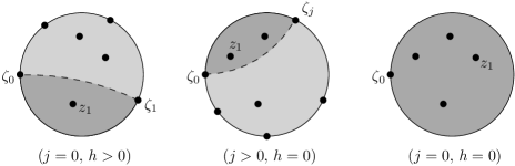
Figure 6.8. The additional terms from (6.3.11).

6.3b. The structure of the argument

To prove compatibility of the cyclic open-closed map and connections, one needs to construct a suitable chain homotopy, which we call an intertwiner. This is a degree $-1$ map, from the cyclic complex of the $q$-deformed Fukaya category, to the $q$-deformed $S^{1}$-equivariant Hamiltonian Floer complex, which satisfies the following equation:

(6.3.13) $$0 =(\text{$q$-deformed equivariant Floer differential})\circ(\text{intertwiner})$$ (i)

$$+(\text{intertwiner})\circ(\text{cyclic homology differential})$$ (ii)

$$+u\partial_{q}(\text{cyclic open-closed map})$$ (iii)

$$+(\text{closed string connection}-u\partial_{q})\circ(\text{cyclic open-closed map})$$ (iv)

$$-(\text{cyclic open-closed map})\circ(\text{modified Getzler-Gauss-Manin}-u\partial_{q}).$$ (v)

In (iii), what we are doing is taking the open-closed map, and differentiating all its coefficients with respect to $q$; as in (6.3.1) this basically means replacing the Maurer-Cartan element at one interior puncture with its derivative $\partial_{q}\alpha$. In (iv) and (v), subtracting $u\partial_{q}$ simply means that we are using all the nontrivial terms in those connections, just ignoring the straightforward differentiation. We have used text since that may be easier to understand, but for actually keeping track of all the terms, we need to replace this by symbols. Recall that the deformed $S^{1}$-equivariant Floer complex (Section 5.3e) is written as $(\mathit{CF}^{*}_{S^{1},q}(H),\delta_{S^{1},q})$. The equation for the intertwiner $\mathit{IT}:\mathit{CC}_{*}^{+}(\mathcal{A}_{q})\rightarrow\mathit{CF}^{*}_{S^{1},q}(H)$ is

(6.3.14) $$0 =\delta_{S^{1},q}\circ\mathit{IT}\qquad\qquad\qquad\qquad\qquad\qquad\quad{}$$ (i)

$$+\mathit{IT}\circ d_{\mathit{CC}_{*}^{+}(\mathcal{A}_{q})}$$ (ii)

$$+u\partial_{q}(\mathit{OC}_{S^{1},q})$$ (iii)

$$+\mathit{KH}\circ\mathit{OC}_{S^{1},q}$$ (iv)

$$-\mathit{OC}_{S^{1},q}\circ(\tilde{\nabla}_{u\partial_{q}}-u\partial_{q}).$$ (v)

(As a consequence of previous notational conventions, certain operations carry a subscript $q$ while others don’t; however, in fact all these structures belong to the $q$-deformed context.)

Following the standard paradigm, the intertwiner is based on moduli spaces whose codimension $1$ degenerations correspond to the terms in the equation above. Recalling that the definition of the closed string connection involved two kinds of moduli spaces labeled (A) and (B), there will be corresponding versions for the intertwiner. Moreover, the open-closed map has two terms labeled (1) and (2), corresponding to the two parts of the cyclic complex, and the intertwiner will also follow the same pattern. This gives a total of four moduli spaces to be defined. The occurrence of boundary terms (i) and (iv) will be geometrically obvious; that of (iii) follows the same idea as in the construction of the closed string connection; and that of (ii) follows the same idea as in the construction of the cyclic open-closed map. Most of the thinking goes into (v), where we need to see how the rather ad-hoc-looking terms in (6.3.12) arise from suitable degenerations. Because of its length, it makes sense to list here how the construction will be set up and organized:

• Geometrically, we will use subsets of the spaces $\mathring{\mathfrak{AH}}_{d,m,r}$ (Section 6.1e), and the same ends and additional data as in the construction of the cyclic open-closed map (Section 6.2d). For this to work, the data are subject to a finite number of additional transversality conditions, which will no longer be stated explicitly.

• For each parameter space, we will list the codimension $1$ boundary strata of the compactification (including ones that were already present as boundary faces of the uncompactified parameter space). In each case, we give an informal description of how points in the interior converge to that stratum, and then if necessary describe the structure of the stratum itself in terms of other moduli spaces (that discussion is not strictly in order; occasionally a space will appear as a boundary stratum before it’s been formally introduced). For those boundary strata that contribute to the terms listed above, we will include (i)–(v) in the notation; those that don’t contribute (because of cancellations) get Roman numerals instead.

• Algebraically, we treat those spaces as in Section 6.3a, but also sum over $r$ (the number of angle decorations) with powers $u^{r}$.

6.3c. Intertwining spaces (A1)

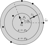
Figure 6.9. A summary of the definition of $\mathring{\mathfrak{AH}}_{d,m,r,w}^{(A1)}$ (as drawn, $d=3$, $m=3$, $r=2$, $w=1$). Due to the authors’ limited drawing skills, the half-cylinder is shown as a disc with the output puncture $z_{0}$ in the center; this will be true of most images in this section.

We take the space from Section 5.2e and marry it to that of Section 6.1f. Fix $d\geq 0$, $m>0$, $r\geq 0$, and $0\leq w\leq r$. Consider half-cylinders (6.1.13) with angle-decorations (6.1.18), and impose a version of (5.2.24) for $z_{1}$, as well as (6.1.21) for $\zeta_{0}$ (Figure 6.9):

(6.3.15) $$z_{1}=(s_{1},t_{1}=\theta_{\geq w+1}),\;\;s_{1}\in\begin{cases}(-\infty,0)&r=0,\\ (-\infty,\sigma_{1}]&w=0,\,r>0\\ [\sigma_{w},\sigma_{w+1}]&w=1,\dots,r-1,\\ [\sigma_{r},0)&w=r,\,r>0,\end{cases}\qquad\zeta_{0}=(0,0).$$

The resulting parameter space is written as $\mathring{\mathfrak{AH}}_{d,m,r,w}^{(A1)}$. The codimension $1$ strata of the compactification are as follows (see Figure 6.10 for the simplest example):

• (A1.1) We can have $\sigma_{i}=\sigma_{i+1}$, for $i\neq w$.

• (A1.2) $s_{1}$ can reach its extremal values: $z_{1}=(\sigma_{w},\theta_{\geq w+1})$ (for $w>0$) or $z_{1}=(\sigma_{w+1},\theta_{\geq w+1})$ (for $w<r$).

• (A1.3) Several interior punctures could collide (at an interior point of the half-cylinder) and form a Fulton-MacPherson bubble. Strictly speaking there are two sub-cases here, depending on whether $z_{1}$ ends up on the bubble or not.

• (A1.i) A cylinder can bubble off at $-\infty$, but where $z_{1}$ remains in the original half-cylinder. The bubble can contain interior punctures as well as angle-decorations, so this stratum is the union of

  (6.3.16) $$\mathring{\mathfrak{AC}}_{m_{1},r_{1}}\times\mathring{\mathfrak{AH}}_{d,m_{2},r_{2},w-r_{1}}^{(A1)},\;\;m_{1}+m_{2}=m,\,r_{1}+r_{2}=r.$$

• (A1.ii) While $z_{1}$ and all angle-decorations remain in the half-cylinder, several punctures (of both kinds) approach a boundary point and bubble off into a punctured disc. This stratum is a union of

  (6.3.17) $$\mathring{\mathfrak{AH}}_{d_{1},m_{1},r,w}^{(A1)}\times\mathring{\mathfrak{R}}_{d_{2},m_{2}},\;\;d_{1}+d_{2}=d+1,\,m_{1}+m_{2}=m.$$

• (A1.ii’) (Only for $w<r$) Suppose that $\sigma_{r}\rightarrow 0$. The principle at work here has already appeared in the construction of the cyclic open-closed map, but we repeat it for convenience. Let $\theta_{i}^{*}$ be the limiting values of $\theta_{i}$ in our degeneration. Take the limiting half-cylinder and rotate it by $-\theta_{r}^{*}$, so that its asymptotic marker points in direction $\theta_{1}^{*}+\cdots+\theta_{r-1}^{*}$. Remove the pieces of parameter space where, after rotation, one of the boundary punctures in the half-cylinder lies at $(0,0)$. The rest can be thought of the disjoint union of components where $(0,0)$ lies between two specific boundary punctures; these are copies of $\mathring{\mathfrak{AH}}^{(A2)}_{d,m,r-1,w}$ where the boundary punctures have been cyclically permuted.

• (A1.iv) (Only for $w=0$) $s_{1}$ can go to $-\infty$, which means that $z_{1}$ bubbles off into a cylinder. This stratum is the union of

  (6.3.18) $$\mathring{\mathfrak{AC}}_{m_{1},r_{1},0}^{(A)}\times\mathring{\mathfrak{AH}}_{d,m_{2},r_{2}}^{(1)},\;\;m_{1}+m_{2}=m,\,r_{1}+r_{2}=r.$$

• (A1.v) (Only for $w=r$, where $\theta_{\geq r+1}=0$) $s_{1}$ can go to $0$, which means that $z_{1}$ approaches the boundary puncture $\zeta_{0}=(0,0)$ along the $\{t=0\}$ axis (perpendicularly to the boundary). The bubble is a punctured disc, where the position of the limit of $z_{1}$ on that disc is constrained to a specific hyperbolic geodesic. One gets the union of

  (6.3.19) $$\mathring{\mathfrak{AH}}^{(1)}_{d_{1},m_{1},r}\times\mathring{\mathfrak{R}}^{0}_{j,1,k,m_{2}},\;\;m_{1}+m_{2}=m,\,d_{1}+j+k=d.$$

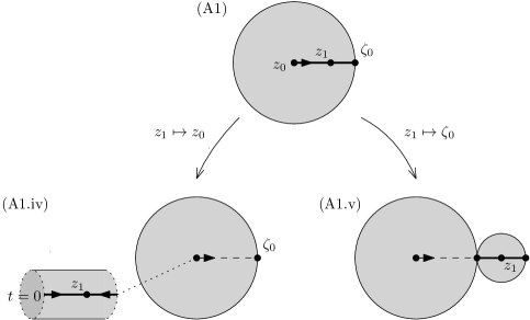
Figure 6.10. For $\mathring{\mathfrak{AH}}_{0,1,0,0}^{(A1)}\cong(0,1)$, only two degenerations can appear.

Remark 6.3.1.

The codimension of strata in the compactification depends on both the number of bubbles and the constraints on the parameter space, and careful consideration of that rules out contributions from many degenerations. For instance, consider the situation where $w=r-1$ and $s_{1}\rightarrow 0$, which necessarily means that $\sigma_{r}\rightarrow 0$ as well. The interior puncture $z_{1}$ approaches the point $(0,\theta_{r})$ and will bubble off into a disc. The remaining half-cylinder carries: the extra boundary puncture at $(0,\theta_{r})$; angle decorations $(\sigma_{1},\theta_{1}),\dots,(\sigma_{r-1},\theta_{r-1})$; and an asymptotic marker at $z_{0}$ rotated by $\theta_{1}+\cdots+\theta_{r}$. Note that these three pieces of data are not independent, and therefore the limit has codimension $2$ (Figure 6.11). In a full compactification, this stratum belongs to the closure of codimension $1$ strata of type (A1.2) and (A1.ii’).

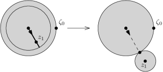
Figure 6.11. The simplest example of the degeneration from Remark 6.3.1. The dimension drops from $3$ (left) to $1$ (right).

Algebraically, the outcome is a map $\mathit{IT}_{(A1)}:C_{*}(\mathcal{A}_{q})[[u]]\rightarrow\mathit{CF}^{*-1}_{S^{1},q}(H)$ which satisfies

(6.3.20) $$0 =\text{(term from $s_{1}$ reaching its extremal values)}$$ (A1.2)

$$\pm\delta_{S^{1},q}\big{(}\mathit{IT}_{(A1)}(a_{0}(a_{1}|\dots|a_{d}))\big{)}$$ (A1.i)

$$\pm\mathit{IT}_{(A1)}\big{(}d_{C_{*}(\mathcal{A}_{q})}(a_{0}(a_{1}|\dots|a_{d}))\big{)}$$ (A1.ii)

$$+u\sum_{j}\pm\mathit{IT}_{(A2)}(e^{+}_{\mathcal{A}}(a_{j}|\dots|a_{j-1}))$$ (A1.ii’)

$$\pm\mathit{KH}_{(A)}\big{(}\mathit{OC}_{S^{1},q,(1)}(a_{0}(a_{1}|\dots|a_{d}))\big{)}$$ (A1.iv)

$$+\sum_{ij}\pm\mathit{OC}_{S^{1},q,(1)}\big{(}\mathit{GM}_{0}^{j,1,k}(a_{d-j+1},\dots,\underline{a_{0}},\dots,a_{k})|a_{k+1}|\dots|a_{d-j}\big{)}$$ (A1.v)

where $d_{C_{*}(\mathcal{A}_{q})}$ is given by the formula (3.2.7). Here, we have tacitly added terms from breaking off of Floer cylinders to (A1.i) and (A1.ii). As usual, the contributions from (A1.3) are zero due to the Maurer-Cartan equation, and those from (A1.1) are zero because that space projects to a lower-dimensional one. We have not given a name to the (A1.2) term, because it will presently turn out to cancel with another term, just as in the definition of the closed string connection (Section 5.3f).

6.3d. Intertwining spaces (B1)

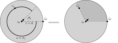
Figure 6.12. Two ways of thinking of the condition (6.3.21), in the simple case of $\mathring{\mathfrak{AH}}_{0,1,1,1}^{(B1)}$. On the left, the marked point $z_{1}$ can lie anywhere on the thickened line. On the right, the asymptotic marker at $z_{0}$ can point into any direction in the darker shaded part of the disc.

We now apply the same idea to the space from Section 5.2f (see Figure 6.12). This means that the first part of (6.3.15) is replaced by (5.2.29), while the second part remains the same. We summarize these conditions for convenience:

(6.3.21) $$\theta_{w}^{\operatorname{lift}}\in[0,1],\;\;\xi\in[\theta_{w}^{\operatorname{lift}},1],\quad z_{1}=(s_{1}=\sigma_{w},\,t_{1}=\theta_{\geq w+1}+\xi),\quad\zeta_{0}=(0,0).$$

This time, examination of the codimension $1$ degenerations in the resulting space $\mathring{\mathfrak{AH}}_{d,m,r,w}^{(B1)}$ is more interesting, see (B1.v) and the even more surprising (B1.v’) below. The full list is:

• (B1.1) We can have $\sigma_{i}=\sigma_{i+1}$ for some $i$.

• (B1.2) We can have $\xi=\theta_{w}^{\operatorname{lift}}$, which means $z_{1}=(\sigma_{w},\theta_{\geq w})$; or $\xi=1$, which means $z_{1}=(\sigma_{w},\theta_{\geq w+1})$.

• (B1.3) We can have bubbling at interior points as in (A1.3).

• (B1.i), (B1.ii), (B1.ii’) as in (A1.i), (A1.ii), (A1.ii’); in the last-mentioned case, the spaces that appear are $\mathring{\mathfrak{AH}}_{d,m,r-1,w}^{(B2)}$.

• (B1.iii) We can have $\theta^{\operatorname{lift}}_{w}=0$, which means that $\xi\in[0,1]$ is arbitrary. By moving $\sigma_{w}$ around, one can then achieve that $z_{1}$ lies anywhere in $[\sigma_{w-1},\sigma_{w+1}]\times S^{1}$ (of course, $t_{1}=\theta_{\geq w+1}$ can be achieved by either setting $\xi=0$ or $\xi=1$, but that is a higher codimension phenomenon and hence irrelevant). One can think of this as part of $\mathring{\mathfrak{R}}_{m,d,r-1}^{(1)}$, and by taking the union over all $w$ one gets all of that space (again, up to higher codimension differences). Looking slightly head, note that while $\mathring{\mathfrak{R}}_{m,d,r-1}^{(1)}$ is the parameter space underlying the term $\mathit{OC}_{(1)}$ of the open-closed map, here we are inserting $\partial_{q}\alpha$ at $z_{1}$, so the algebraic contribution will in fact be $\partial_{q}\mathit{OC}_{(1)}$.

• (B1.iv) as in (A1.iv).

• (B1.v) (This only applies to $w=r$, in which case $\theta_{\geq r+1}=0$) Suppose we have $\sigma_{r}\rightarrow 0$, and that $\xi$ also converges to some $\xi^{*}\in(0,1)$; more geometrically, $z_{1}$ approaches the boundary point $(0,\xi^{*})\neq\zeta_{0}=(0,0)$, and will bubble off into a punctured disc. Assume moreover that $\theta_{r}^{\operatorname{lift}}$ approaches some limit

  (6.3.22) $$\theta_{r}^{\operatorname{lift},*}\in(0,\xi^{*}).$$

  Note that on the boundary of the half-cylinder, the points $(0,0)$, $(0,\theta_{r}^{\operatorname{lift},*})$, $(0,\xi^{*})$ appear in that cyclic order.

  In the limiting half-cylinder, $(0,\xi^{*})$ becomes a boundary puncture. Between $(0,0)$ and that can lie other boundary punctures, but removing higher codimension pieces, we can assume that none of those punctures equals $(0,\theta_{r}^{\operatorname{lift},*})$; then the outcome can be subdivided into cases, depending on the boundary punctures that are on either side of the point $(0,\theta_{r}^{\operatorname{lift},*})$. Let’s mentally rotate the half-cylinder by $-\theta_{r}^{\operatorname{lift},*}$, so that those punctures end up on either side of $(0,0)$, and cyclically permute the labels so that the two punctures now appear as the last and first one in our order. Altogether, this yields boundary faces of the form (Figure 6.13)

  (6.3.23) $$\mathring{\mathfrak{AH}}_{d_{1},m_{1},r-1}^{(2)}\times\mathring{\mathfrak{R}}_{d_{2},m_{2}},\;\;d_{1}+d_{2}=d+1,m_{1}+m_{2}=m.$$

  Let’s remind ourselves that one of the $m_{2}$ interior marked points on the disc component is the limit of $z_{1}$. Algebraically, this carries $\partial_{q}\alpha$, which means that the contribution from the disc component will be $\partial_{q}\mu_{q}$. Note that in the new ordering of boundary punctures on the half-cylinder, the puncture $(0,\xi^{*}-\theta_{r}^{\operatorname{lift},*})$ where the disc bubble is attached appears before $(0,-\theta_{r}^{\operatorname{lift},*})$; This is a consequence of the previous observation concerning cyclic order, and will effect an asymmetry in the algebraic contribution, where the $\partial_{q}\mu_{q}$ term appears before the $0$-th entry of the Hochschild chain.

  

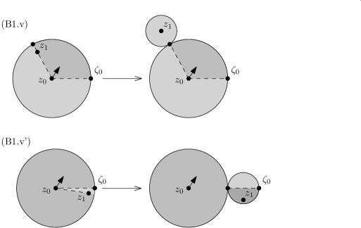
  Figure 6.13. The degenerations of type (B1.v) and (B1.v’), drawn in the same way as the right part of Figure 6.12.

• (B1.v’) (This also only applies to $w=r$.) Suppose that $\sigma_{r}\rightarrow 0$ and $\xi\rightarrow 1$, but in such that $\sigma_{r}/(1-\xi)$ approaches a nonzero (and then necessarily negative) limit. This means that $z_{1}\rightarrow(0,0)$, but the approach is from below the line $\{t=0\}$ and at some nonzero slope. It is instructive to think of the resulting disc bubble as the left half-plane obtained by rescaling the situation near $(0,0)$. Then, the limit of $z_{1}$ lies in the left lower quarter-plane (Figure 6.14). In more intrinsic terms, it lies below the hyperbolic geodesic connecting two specific punctures in the bubble.

  

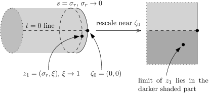
  Figure 6.14. An alternative picture of the bubbling from (B1.v’), showing it as a rescaling process.

  Note that in this situation, $\theta_{r}^{\mathrm{lift}}$ can converge to an arbitrary limit, since any value is compatible with $\xi\rightarrow 1$. The half-cylinder component of the limit is then treated as in (A1.ii’). Ignoring higher codimension pieces, one can think of the outcome as copies of

  (6.3.24) $$\mathring{\mathfrak{AH}}_{d_{1},m_{1}}^{(2)}\times\mathring{\mathfrak{R}}^{-}_{j,1,k,m_{2}},\;\;j+k+d_{1}=d,\;m_{1}+m_{2}=m,$$

  summing over those cyclic permutations of the boundary punctures such that the limit of the $0$-th input remains on bubble ($\mathfrak{R}^{-}$) component.

Remark 6.3.2.

Again, there are other strata in which only one bubble component exists, but which are of higher codimension due to restriction on the parameter. For instance, consider $w=r$ and the limit where $\sigma_{r}\rightarrow 0$ and $\xi\rightarrow 0$ (which necessarily means that $\theta_{r}^{\mathrm{lift}}\rightarrow 0$ as well). In that limit, the marked point $z_{1}$ approaches $(0,0)$ from above the axis $t=0$, so we get a limit with a position constraint in the bubble, as in Figure 6.15. However, simple dimension-counting shows that this stratum is of codimension $2$.

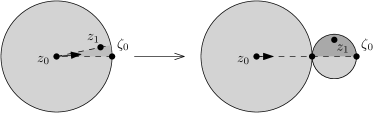
Figure 6.15. The limit from Remark 6.3.2, in the simplest case of $\mathring{\mathfrak{AH}}_{0,1,1,1}^{(B1)}$. We again follow the drawing conventions from the right part of Figure 6.12.

The outcome is an operation $\mathit{IT}_{(B1)}:C_{*}(\mathcal{A}_{q})[[u]]\rightarrow\mathit{CF}^{*-1}_{S^{1},_{q}}(H)$ which satisfies

(6.3.25) $$0 =\text{(term from $\xi$ reaching its extremal values)}$$ (B1.2)

$$\pm\delta_{S^{1},q}\big{(}\mathit{IT}_{(B1)}(a_{0}(a_{1}|\dots|a_{d}))\big{)}$$ (B1.i)

$$\pm\mathit{IT}_{(B1)}\big{(}d_{C_{*}(\mathcal{A}_{q})}(a_{0}(a_{1}|\dots|a_{d}))\big{)}$$ (B1.ii)

$$+u\sum_{j}\pm\mathit{IT}_{(B2)}(e^{+}_{\mathcal{A}}(a_{j}|\dots|a_{j-1}))$$ (B1.ii’)

$$\pm(u\partial_{q}\mathit{OC}_{S^{1},q,(1)})(a_{0}(a_{1}|\dots|a_{d}))$$ (B1.iii)

$$\pm\mathit{KH}_{(B)}\big{(}\mathit{OC}_{S^{1},q,(1)}(a_{0}(a_{1}|\dots|a_{d}))\big{)}$$ (B1.iv)

$$+u\sum_{ijk}\pm\mathit{OC}_{S^{1},q,(2)}\big{(}e_{\mathcal{A}}^{+}(a_{i+1}|\dots|$$

$$\qquad\qquad\qquad\partial_{q}\mu_{q}^{k}(a_{j+1},\dots,a_{j+k})|\dots|a_{0}|\dots|a_{i})\big{)}$$ (B1.v)

$$+u\sum_{ijk}\pm\mathit{OC}_{S^{1},q,(2)}\big{(}e^{+}_{\mathcal{A}}\otimes(a_{i+1}|\dots|$$

$$\qquad\qquad\qquad\mathit{GM}_{-}^{l-j,1,k}(a_{j+1},\dots,\underline{a_{0}},\dots,a_{k})|\dots|a_{i})\big{)} \text{(B1.v')}.$$

The (A1.2) and (B1.2) terms in (6.3.20) and (6.3.25) concern the same surfaces. Hence, if we consider the sum $\mathit{IT}_{(A1)}+\mathit{IT}_{(B1)}$, they will cancel, in parallel with the construction of the closed string connection (Section 5.3f).

6.3e. Intertwining spaces (A2)

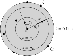
Figure 6.16. The counterpart of Figure 6.9 for $\mathring{\mathfrak{AH}}_{d,m,r,w}^{(A2)}$. We remind the reader that in this context, $(0,0)$ is not a puncture.

We now apply the same treatment as in Section 6.3c to the second part of the cyclic open-closed map. It is worth while writing down the constraints (Figure 6.16):

(6.3.26) $$z_{1}=(s_{1},t_{1}=\theta_{\geq w+1}),\;\;s_{1}\in\begin{cases}(-\infty,0)&r=0,\\ (-\infty,\sigma_{1}]&w=0,\,r>0\\ [\sigma_{w},\sigma_{w+1}]&w=1,\dots,r-1,\\ [\sigma_{r},0)&w=r,\,r>0,\end{cases}$$

$$(0,0)\text{ lies in the closed interval in $\{0\}\times S^{1}$ starting at $\zeta_{d}$ and ending at $\zeta_{1}$.}$$

Here are the codimension $1$ degenerations of the resulting space $\mathring{\mathfrak{AH}}^{(A2)}_{d,m,r,w}$:

• (A2.1–3), (A2.i) as in (A1.1–3), (A1.i).

• (A2.ii) While $z_{1}$ and all angle-decorations remain in the half-cylinder, several punctures (of both kinds) approach a boundary point and bubble off into a punctured disc; but at most one of $(\zeta_{1},\zeta_{d})$ can belong to this group of colliding points. This stratum is a union of

  (6.3.27) $$\mathring{\mathfrak{AH}}_{d_{1},m_{1},r,w}^{(A2)}\times\mathring{\mathfrak{R}}_{d_{2},m_{2}},\;\;d_{1}+d_{2}=d+1,\,m_{1}+m_{2}=m.$$

• (A2.ii’) The condition on $(\zeta_{1},\zeta_{d})$ in (6.3.26) achieves its extrema, which means that either $\zeta_{1}=(0,0)$ or $\zeta_{d}=(0,0)$. In either case, we have arrived at (6.3.15) where the role of $\zeta_{0}$ is played by either $\zeta_{1}$ or $\zeta_{d}$, and with the remaining boundary punctures cyclically reordered; so this boundary stratum consists of two copies of $\mathring{\mathfrak{AH}}_{d,m,r,w}^{(A1)}$.

• (A2.iv) as in (A1.iv).

• (A2.v) (Only for $w=r$) we can have $s_{1}\rightarrow 0$, which means $z_{1}\rightarrow(0,0)$, but where both boundary punctures $\zeta_{1}$ and $\zeta_{d}$ stay away from the limiting point $(0,0)$. This creates a disc bubble with a single interior puncture (the limit of $z_{1}$) and only one boundary puncture. The outcome is

  (6.3.28) $$\mathring{\mathfrak{AH}}_{d+1,m-1,r}^{(1)}\times\mathring{\mathfrak{R}}_{0,1}.$$

  (For this and the following degenerations, see Figure 6.17.)

  

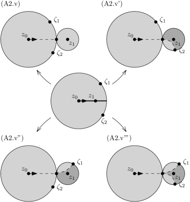
  Figure 6.17. Four related (A2) degenerations. In each case, the possible positions of $z_{1}$ on the bubble are in the darker shaded region.

• (A2.v’) (Also only for $w=r$) We have $s_{1}\rightarrow 0$ as before, but this time some collection of points $(\zeta_{d-j+2},\dots,\zeta_{d})$ approaches $(0,0)$ from the direction of $t<0$, in such a way that their limits as well as the limit of $z_{1}$ lie on the resulting bubble. As a consequence of the original condition on the positions of $z_{1}$ and $\zeta_{d}$, the points on the bubble inherit a constraint, which makes the stratum

  (6.3.29) $$\mathring{\mathfrak{AH}}_{d-j+1,m_{1},r}^{(1)}\times\mathring{\mathfrak{R}}_{j-1,1,0,m_{2}}^{+},\;\;m_{1}+m_{2}=m.$$

• (A2.v”) (Also only for $w=r$) Similar, but with $(\zeta_{1},\dots,\zeta_{h-1})$ which approach $(0,0)$ from the direction of $t>0$. The resulting stratum has the form

  (6.3.30) $$\mathring{\mathfrak{AH}}_{d-h+1,m_{1},r}^{(1)}\times\mathring{\mathfrak{R}}_{0,1,h-1,m_{2}}^{-},\;\;m_{1}+m_{2}=m.$$

• (A2.v”’) (Also only for $w=r$) Finally, as $s_{1}\rightarrow 0$, we can have two groups of boundary punctures apprach $(0,0)$, one from each direction. This leads to boundary strata

  (6.3.31) $$\mathring{\mathfrak{AH}}_{d-h-j+1,m_{1},r}^{(1)}\times\mathring{\mathfrak{R}}_{j,h,m_{2}}^{\prec},\;\;m_{1}+m_{2}=m.$$

  It is maybe better to think of the bubble as appearing through rescaling (Figure 6.18). On the original half-cylinder, $z_{1}$ lies between two lines bounded by $\zeta_{d}$ and $\zeta_{1}$. After rescaling, we see the same phenomenon happening on the bubble half-plane, where the lines are now hyperbolic geodesics.

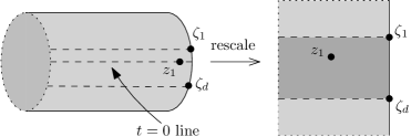
Figure 6.18. An alternative picture of the (A2.v’”) degeneration.

Remark 6.3.3.

In (A2.ii) we have not considered the case where $\zeta_{1}$ and $\zeta_{d}$ collide; such a collision can only occur at $(0,0)$, making the resulting stratum codimension $2$.

The outcome is an operation $\mathit{IT}_{(A2)}:e^{+}_{\mathcal{A}}\otimes B(\mathcal{A}_{q})[[u]]\rightarrow\mathit{CF}^{*-2}_{S^{1},q}(H)$ which satisfies

(6.3.32) $$0 =\text{(term from $s_{1}$ reaching its extremal values)}$$ (A2.2)

$$\pm\delta_{S^{1},q}\big{(}\mathit{IT}_{(A2)}(e^{+}_{\mathcal{A}}(a_{1}|\dots|a_{d}))\big{)}$$ (A2.i)

$$\pm\mathit{IT}_{(A2)}\big{(}e^{+}_{\mathcal{A}}\,d_{D_{*}(\mathcal{A}_{q})}(a_{1}|\dots|a_{d})\big{)}$$ (A2.ii)

$$\pm\mathit{IT}_{(A1)}\big{(}a_{1}(a_{2}|\dots|a_{d})\big{)}\pm\mathit{IT}_{(A1)}\big{(}a_{d}(a_{1}|\dots|a_{d-1})\big{)}$$ (A2.ii’)

$$\pm\mathit{KH}_{(A)}\big{(}\mathit{OC}_{S^{1},q,(2)}(e^{+}_{\mathcal{A}}(a_{1}|\dots|a_{d}))\big{)}$$ (A2.iv)

$$\pm\mathit{OC}_{S^{1},q,(1)}\big{(}\mathit{GM}^{0,0}_{\prec}\,(a_{1}|\dots|a_{d})\big{)}$$ (A2.v)

$$+\sum_{j}\pm\mathit{OC}_{S^{1},q,(1)}\big{(}\mathit{GM}^{j,0}_{\prec}(a_{d-j+1},\dots,a_{l})(a_{1}|\dots|a_{d-j})\big{)}$$ (A2.v’)

$$+\sum_{h}\pm\mathit{OC}_{S^{1},q,(1)}\big{(}\mathit{GM}^{0,h}_{\prec}(a_{1},\dots,a_{h})(a_{h+1}|\dots|a_{d})\big{)}$$ (A2.v”)

$$+\sum_{j,h>0}\pm\mathit{OC}_{S^{1},q,(1)}\big{(}\mathit{GM}^{j,h}_{\prec}(a_{l-j+},\dots,a_{d},a_{1},\dots,a_{h})(a_{h+1}|\dots|a_{d-j})\big{)}$$ (A2.v”’)

where $d_{D_{*}(\mathcal{A}_{q})}$ is given by the formula from (3.2.22) (applied to the deformed $A_{\infty}$-structure of $\mathcal{A}_{q}$, of course). The last four terms in (6.3.32) appear algebrically the same, but that’s because we have applied (6.3.11) to slightly different geometric situations.

6.3f. Intertwining spaces (B2)

Our final space $\mathring{\mathfrak{AH}}_{d,m,r,w}^{(B2)}$ imposes the following conditions on $z_{1}$ and the boundary punctures:

(6.3.33) $$\theta_{w}^{\operatorname{lift}}\in[0,1],\;\;\xi\in[\theta_{w}^{\operatorname{lift}},1],\quad z_{1}=(s_{1}=\sigma_{w},\,t_{1}=\theta_{\geq w+1}+\xi),$$

$$(0,0)\text{ lies in the closed interval in $\{0\}\times S^{1}$ starting at $\zeta_{d}$ and ending at $\zeta_{1}$.}$$

There is nothing fundamentally new in the codimension $1$ degenerations:

• (B2.1-3), (B2.i) as in (B1.1-3), BA1.i).

• (B2.ii-ii’) as in (A2.ii-ii’).

• (B2.iii) as in (B1.iii).

• (B2.iv) as in (A1.iv).

Remark 6.3.4.

As in the construction of $\mathit{OC}_{(2)}$, the limit $s_{1}\rightarrow 0$ does not contribute anything. The case not covered by previous considerations is $w=r$, where $s_{1}\rightarrow 0$ means that $z_{1}$ approaches the boundary. However, this is again just a dimension count. Consider the simplest example $d=2$, $m=1$, $r=1$. The space $\mathfrak{AH}_{2,1,1,1}^{(B2)}$ has dimension $5$. (The degrees of freedom are: the positions of the two boundary marked points; the angle-decoration $(\sigma_{1},\theta_{1})$; and the position of $z_{1}$ on the circle $s=\sigma_{1}$. Note that we are not dividing by the $S^{1}$-action which rotates the half-cylinder, since that would break the condition that the asymptotic marker at $z_{0}=-\infty$ is rotated by $\theta_{1}$ with respect to the $t=0$ line.) The limit (Figure 6.19) is a half-cylinder with three boundary punctures, together with a bubble component that is a disc with one boundary puncture and one interior puncture. At this point, we rotate the half-cylinder by $-\theta_{1}$ to bring the marker back into standard position, and then the outcome belongs to a $3$-dimensional parameter spaces. (Other limit configurations are possible, even in this simple situation, but the codimension argument still holds for those.)

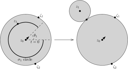
Figure 6.19. The degeneration in $\mathring{\mathfrak{AH}}_{2,1,1,1}$ discussed in Remark 6.3.4.

Given that, the operation $\mathit{IT}_{(B2)}:e^{+}_{\mathcal{A}}\otimes B(\mathcal{A}_{q})[[u]]\longrightarrow\mathit{CF}^{*-2}_{S^{1},q}(H)$ satisfies

(6.3.34) $$0 =\text{(term from $\xi$ reaching its extremal values)}$$ (B2.i)

$$\pm\delta_{S^{1},q}\big{(}\mathit{IT}_{(B2)}(e^{+}_{\mathcal{A}}(a_{1}|\dots|a_{d}))\big{)}$$ (B2.i)

$$\pm\mathit{IT}_{(B2)}\big{(}e^{+}_{\mathcal{A}}\,d_{D_{*}(\mathcal{A}_{q})}(a_{1}|\dots|a_{d})\big{)}$$ (B2.ii)

$$\pm\mathit{IT}_{(B1)}\big{(}a_{1}(a_{2}|\dots|a_{d})\pm a_{d}(a_{1}|\dots|a_{d-1})\big{)}$$ (B2.ii’)

$$\pm(u\partial_{q}\mathit{OC}_{S^{1},q,(2)})(e_{\mathcal{A}}^{+}(a_{1}|\dots|a_{d}))$$ (B2.iii)

$$\pm\mathit{KH}_{(B)}\big{(}\mathit{OC}_{S^{1},q,(2)}(e_{\mathcal{A}}^{+}(a_{1}|\dots|a_{d}))\big{)}$$ (B2.iv)

6.3g. Conclusion

Write $\mathit{IT}_{(1)}=\mathit{IT}_{(A1)}\pm\mathit{IT}_{(B1)}$ and $\mathit{IT}_{(2)}=\mathit{IT}_{(A2)}\pm\mathit{IT}_{(B2)}$. By adding up (6.3.20) and (6.3.25) one sees that

(6.3.35) $$0 =\pm\delta_{S^{1},q}(\mathit{IT}_{(1)}(a_{0}(a_{1}|\dots|a_{d})))$$ (A1+B1.i)

$$\pm\mathit{IT}_{(1)}(d_{C_{*}(\mathcal{A}_{q})}(a_{0}(a_{1}|\dots|a_{d})))$$ (A1+B1.ii)

$$+u\sum_{j}\pm\mathit{IT}_{(2)}(e^{+}_{\mathcal{A}}(a_{j}|\dots|a_{j-1}))$$ (A1+B1.ii’)

$$\pm(u\partial_{q}\,\mathit{OC}_{S^{1},q,(1)})(a_{0}(a_{1}|\dots|a_{d}))$$ (B1.iii)

$$\pm\mathit{KH}\big{(}\mathit{OC}_{S^{1},q,(1)}(a_{0}(a_{1}|\dots|a_{d}))\big{)}$$ (A1+B1.iv)

$$+\sum_{ij}\pm\mathit{OC}_{S^{1},q,(1)}(\mathit{GM}_{0}^{j,1,k}(a_{d-j+1},\dots,\underline{a_{0}},\dots,a_{k})|$$

$$\qquad\qquad\qquad a_{k+1}|\dots|a_{d-j})$$ (A1.v)

$$+u\sum_{ijk}\pm\mathit{OC}_{S^{1},q,(2)}\big{(}e_{\mathcal{A}}^{+}(a_{i+1}|\dots|$$

$$\qquad\qquad\qquad\partial_{q}\mu_{q}^{k}(a_{j+1},\dots,a_{j+k})|\dots|a_{0}|\dots|a_{i})\ ib)$$ (B1.v)

$$+u\sum_{ijk}\pm\mathit{OC}_{S^{1},q,(2)}\big{(}e^{+}_{\mathcal{A}}\otimes(a_{i+1}|\dots|$$

$$\qquad\qquad\qquad\mathit{GM}_{-}^{l-j,1,k}(a_{j+1},\dots,\underline{a_{0}},\dots,a_{k})|\dots|a_{i})\big{)}$$ (B1.v’)

Similarly, adding up (6.3.32) and (6.3.34) yields

(6.3.36) $$0 =\pm\delta_{S^{1},q}\big{(}\mathit{IT}_{(2)}(e_{+}(a_{1}|\dots|a_{d}))\big{)}$$ (A2+B2.i)

$$\pm\mathit{IT}_{(2)}\big{(}e^{+}_{\mathcal{A}}\,d_{D_{*}(\mathcal{A}_{q})}(a_{1}|\dots|a_{d})\big{)}$$ (A2+B2.ii)

$$\pm\mathit{IT}_{(1)}\big{(}a_{1}(a_{2}|\dots|a_{d})\big{)}\pm\mathit{IT}_{(1)}\big{(}a_{d}(a_{2}|\dots|a_{d-1})\big{)}$$ (A2+B2.ii’)

$$\pm(u\partial_{q}\,\mathit{OC}_{S^{1},q,(2)})(e^{+}_{\mathcal{A}}(a_{1}|\dots|a_{d}))$$ (B2.iii)

$$\pm\mathit{KH}\big{(}\mathit{OC}_{S^{1},q,(2)}(e_{\mathcal{A}}^{+}(a_{1}|\dots|a_{d}))\big{)}$$ (A2+B2.iv)

$$+\sum_{jh}\pm\mathit{OC}_{S^{1},q,(1)}\big{(}\mathit{GM}_{\prec}^{j,h}(a_{l-j+1},\dots,a_{l},a_{1},\dots,a_{h})(a_{h+1}|\dots|a_{l-j})\big{)}$$ (A2.v-v”’)

The equations (6.3.35), (6.3.36) are exactly what one gets by spelling out (6.3.14) using the formulae for the differential on the cyclic complex (3.2.26) and the modified Gauss-Manin connection (6.3.12). We have now shown that (6.3.14) holds. Since $\tilde{\nabla}_{u\partial_{q}}$ is chain homotopic to $\nabla_{u\partial_{q}}$ by definition, the outcome is:

Theorem 6.3.5.

For any Maurer-Cartan element (5.3.25) and the associated deformation $\mathcal{A}_{q}$ of $\mathcal{A}$, the following diagram commutes up to chain homotopy:

(6.3.37)

7. The complement of a smooth anticanonical divisor

Whereas before we worked with general Liouville manifolds, here we use specific geometric properties of the complement of a smooth anticanonical divisor, and their implications for Floer cohomology. We describe the overall algebraic argument first, since that brings together tools from all the different parts of the paper, leading to the proof of our main results (in Section 7.1c). After that, we go back to geometry for the necessary ingredients (which are all present in the literature, so that is more of a summary).

The concluding Section 7.3 is of a different nature. It can be considered as a comment on the conjectures about deformed symplectic cohomology that enter into the argument, and the conclusions we have drawn from them. Namely, we discuss a canodidate toy model, constructed in terms of differential forms, intended to describe the theory if there were no rational curves in the pair $(M,D)$. We have not tried to show that this candidate is correct, which would be quixotic anyway since no such examples are known; however, this kind of “before quantum corrections” thinking can still potentially be useful, in order to understand the conjectures better.

7.1. Finiteness results

7.1a. Symplectic cohomology

Let $(M,D)$ be as in Assumption 1.2.1. Let $K_{M}^{-1}=\lambda^{\mathrm{top}}_{{\mathbb{C}}}(TM)$ be the anticanonical line bundle, for some compatible almost complex structure. The assumption on $[D]$ says that we can find a smooth section of $K_{M}^{-1}$ which vanishes exactly along $D$. From that, $M\setminus D$ inherits a trivialization of its anticanonical bundle. Next, because $[D]=[\omega_{M}]$, one can turn the complement of a suitable tubular neighbourhood of $D$ into a Liouville domain $N$, and then complete that to $\hat{N}$ (this is standard, but see Section 7.2a for an exposition).

Notation 7.1.1.

Write $C$ for the Hamiltonian Floer complex on $\hat{N}$, and $H$ for its cohomology. (In the notation of Section 4.1e, $C=\mathit{CF}^{*}(H)$; and in standard symplectic topology notation, see e.g. [76], $H=\mathit{SH}^{*}(\hat{N})$.) One can achieve the following, which we will assume to be the case from now on: $C$ is concentrated in nonnegative degrees, and its cohomology is concentrated in degrees $\leq\mathrm{dim}_{{\mathbb{R}}}(M)-1$ (one can even get a little more, see Proposition 7.2.1).

Recall that $H$ is a graded commutative ring. From the compactification $M$, we inherit a distinguished class in $H^{0}$, called here the Borman-Sheridan class $b$ (this is a well-known construction, see Section 7.2 for references).

Lemma 7.1.2.

(This is a consequence of results from [35], see Section 7.2 for details) $H$ is a finitely generated ${\mathbb{K}}[t]$-module, where $t$ acts by multiplication with $b$.

In view of our boundedness assumption, $b$ has a unique cocycle representative, denoted by $\beta\in C^{0}$. The element

(7.1.1) $$\alpha=q\beta\in qC[q]$$

is automatically Maurer-Cartan for the $L_{\infty}$-structure on $C[1]$ from Section 5.3a, since all the nonlinear terms in (3.4.10) vanish for degree reasons: if $m\geq 2$, $\ell^{m}(\alpha,\dots,\alpha)=q^{m}\ell^{m}(\beta,\dots,\beta)\in q^{m}C^{3-2m}=0$.

Notation 7.1.3.

Write $C_{q}$ for the space $C[q]$ equipped with the differential deformed by $\alpha$ (in the notation of Definition 5.3.7(ii), $C_{q}=\mathit{CF}^{*}_{q}(H)$; note there’s no distinction between polynomials and power series in $q$, because $C$ is bounded below). Write $H_{q}$ for its cohomology. $H_{q}$ has the structure of a ${\mathbb{K}}[q,t]$-module, where the degree $0$ variable $t$ acts as $\iota_{q}$, as defined in (5.3.40).

The map $H_{q}\rightarrow H$ obtained by setting $q=0$ is $t$-linear, essentially by definition. Namely, the only term in (5.3.40) not containing any $q$ is the one with $m=0$, and $\mathit{KH}^{(A)}_{1,0}(\partial_{q}\alpha,\cdot)=\mathit{KH}^{(A)}_{1,0}(\beta,\cdot)$ is the pair-of-pants product with the Borman-Sheridan class (see Example 5.3.9).

Lemma 7.1.4.

$H_{q}$ is a finitely generated ${\mathbb{K}}[q,t]$-module.

Proof.

The long exact sequence

(7.1.2) $$\cdots\rightarrow H_{q}^{*-2}\stackrel{{\scriptstyle q}}{{\longrightarrow}}H_{q}\stackrel{{\scriptstyle q=0}}{{\longrightarrow}}H\rightarrow\cdots$$

shows that $H_{q}/qH_{q}$ injects into $H$. Hence, by Lemma 7.1.2, $H_{q}/qH_{q}$ is finitely generated over ${\mathbb{K}}[t]$. Pick generators $\bar{h}_{1},\dots,\bar{h}_{k}\in H_{q}/qH_{q}$, and lifts $h_{1},\dots,h_{k}$ to $H_{q}$. Without loss of generality, we can assume that those are homogeneous (each lies in a fixed degree). Given some $x\in H_{q}^{d}$ with image $\bar{x}\in(H_{q}/qH_{q})^{d}$, one can write

(7.1.3) $$\bar{x}=\sum_{\begin{subarray}{c}j\in\{1,\dots,k\}\\ \text{such that }|\bar{h}_{j}|=d\end{subarray}}f_{j}(t)\bar{h}_{j},\quad\text{with $f_{j}(t)\in{\mathbb{K}}[t]$.}$$

This means that

(7.1.4) $$x-\!\!\!\!\!\!\!\!\!\sum_{\begin{subarray}{c}j\in\{1,\dots,k\}\\ \text{such that }|h_{j}|=d\end{subarray}}f_{j}(t)h_{j}(t)\in qH_{q}^{d-2}.$$

We can write the difference (7.1.4) as $q\tilde{x}$, apply the same argument to $\tilde{x}$, and then iterate to get an expression for $x$ as a ${\mathbb{K}}[q,t]$-linear combination of the $h_{j}$ (because $H_{q}$ is bounded below, the process terminates after finitely many iterations). ∎

The argument above, and its cousins yet to follow, could be formulated more concisely in spectral sequence terms; but we prefer to avoid that language, in order to make (the absence of) convergence issues as clear as possible.

Conjecture 7.1.5.

${\mathbb{K}}[q^{\pm 1}]\otimes_{{\mathbb{K}}[q]}H_{q}$ is a finitely generated ${\mathbb{K}}[q^{\pm 1}]$-module (or equivalently, it is of finite dimension over ${\mathbb{K}}$ in each degree).

Lemma 7.1.6.

If Conjecture 7.1.5 holds, there is a nonzero $p(t)\in{\mathbb{K}}[t]$ and an $r\in{\mathbb{N}}$ such that $p(t)q^{r}$ acts trivially on $H_{q}$.

Proof.

Because $t$ is an endomorphism of the finite-dimensional ${\mathbb{K}}$-vector space $H_{q,q^{-1}}^{0}\oplus H_{q,q^{-1}}^{1}$, there must be some $p$ such that $p(t)$ acts trivially there. By multiplication with powers of $q$, one sees that $p(t)$ acts trivially on all of $H_{q,q^{-1}}$. Let $h_{1},\dots,h_{k}$ be generators of $H_{q}$ over ${\mathbb{K}}[q,t]$ (Lemma 7.1.4). The previous argument shows that $p(t)h_{j}$ is $q$-torsion for each $j$. Therefore, there is some $r$ such that $q^{r}p(t)h_{j}=0$ for all $j$. ∎

Lemma 7.1.7.

If Conjecture 7.1.5 holds, ${\mathbb{K}}(t)\otimes_{{\mathbb{K}}[t]}H_{q}$ is finite-dimensional over ${\mathbb{K}}(t)$ in each degree, and vanishes in sufficiently high degrees.

Proof.

The finite generation statement from Lemma 7.1.4 clearly implies that in each degree, $H_{q}$ is a finitely generated ${\mathbb{K}}[t]$-module, which is stronger than the corresponding ${\mathbb{K}}(t)$ statement. For the second part, let’s use Lemma 7.1.4 more explicitly, choosing homogeneous generators $h_{1},\dots,h_{k}$ of $H_{q}$ over ${\mathbb{K}}[t,q]$. Given any $x\in H_{q}^{d}$, one can write

(7.1.5) $$x=\!\!\!\!\!\!\sum_{\begin{subarray}{c}j\in\{1,\dots,k\}\\ \text{such that }d-|h_{j}|\\ \text{is $\geq 0$ and even}\end{subarray}}q^{(d-|h_{j}|)/2}f_{j}(t)h_{j}\quad\text{with $f_{j}(t)\in{\mathbb{K}}[t]$}.$$

As $d$ gets larger, it follows that $x$ is divisible by higher and higher powers of $q$. For sufficiently large $d$, Lemma 7.1.6 then shows that $p(t)x=0$, which means that $x$ becomes zero in ${\mathbb{K}}(t)\otimes_{{\mathbb{K}}[t]}H_{q}$. ∎

Notation 7.1.8.

Write $C_{u}$ for the $S^{1}$-equivariant Floer complex, which means that it’s $C[u]$ with a $u$-deformation of the previous Floer differential ($C_{u}=\mathit{CF}^{*}_{S^{1}}(H)$ in the notation of Section 5.3c, where this is constructed; again, the difference between polynomials and power series is irrelevant for grading reasons). Let $H_{u}$ be its cohomology ($H_{u}=\mathit{SH}^{*}_{S^{1}}(\hat{N})$ in standard symplectic topology notation).

As before, there is a deformation induced by (7.1.1), denoted by $C_{q,u}$, with underlying ${\mathbb{K}}[q,u]$-module $C[q,u]$ (this is $C_{q,u}=\mathit{CF}^{*}_{S^{1},q}(H)$ from Section 5.3e). We write $H_{q,u}$ for the cohomology of $C_{q,u}$. The action of $u$, $q$, and the closed string connection $t=\nabla_{u\partial_{q}}$ (constructed in Section 5.3f) make $C_{q,u}$ into a complete and $u$-torsionfree $W_{q,u}$-module, in the sense of Section 2.3.

The map $H_{q,u}\rightarrow H_{q}$ obtained by setting $u=0$ relates the $W_{q,u}$-module structure on $H_{q,u}$ with the ${\mathbb{K}}[q,t]$-module structure on $H_{q}$, by (5.3.41).

Lemma 7.1.9.

$H_{q,u}$ is finitely generated over $W_{q,u}$.

Proof.

The long exact sequence

(7.1.6) $$\cdots\rightarrow H_{q,u}[-2]\stackrel{{\scriptstyle u}}{{\longrightarrow}}H_{q,u}\stackrel{{\scriptstyle u=0}}{{\longrightarrow}}H_{q}\rightarrow\cdots$$

shows that $H_{q,u}/uH_{q,u}$ injects into $H_{q}$, hence is finitely generated over ${\mathbb{K}}[q,t]$ by Lemma 7.1.4. Pick homogeneous generators $\bar{h}_{1},\dots,\bar{h}_{k}\in H_{q,u}/uH_{q,u}$, and lifts $h_{1},\dots,h_{k}$ to $H_{q,u}$. Given some $x\in H_{q,u}^{d}$ with image $\bar{x}\in H_{q,u}/uH_{q,u}d$, one proceeds as in (7.1.5),

(7.1.7) $$\bar{x}=\!\!\!\!\!\!\!\sum_{\begin{subarray}{c}j\in\{1,\dots,k\}\\ \text{such that }d-|h_{j}|\\ \text{is $\geq 0$ and even}\end{subarray}}\!\!\!\!\!\!\!q^{(d-|h_{j}|)/2}\bar{f}_{j}(t)\bar{h}_{j},\quad\text{with $\bar{f}_{j}(q,t)\in{\mathbb{K}}[t]$.}$$

Take $f_{j}=q^{(d-|h_{j}|)/2}\bar{f}_{j}(t)\in W_{q,u}$ (one could also choose any other element $f_{j}$ of $W_{q,u}$ of the same degree and with the same $u=0$ reduction). Then

(7.1.8) $$x-\!\!\!\!\!\!\!\sum_{\begin{subarray}{c}j\in\{1,\dots,k\}\\ \text{such that }d-|h_{j}|\\ \text{is $\geq 0$ and even}\end{subarray}}\!\!\!\!\!\!\!f_{j}(t)h_{j}\in uH_{q,u}^{d-2}.$$

Writing this as $u\tilde{x}$, one then iterates as in the proof of Lemma 7.1.4. ∎

The next two statements yield an analogue (in the $W_{q,u}$-context) of the classical idea that finitely generated modules over the Weyl algebra are holonomic if and only if they have one-dimensional singular support.

Lemma 7.1.10.

If Conjecture 7.1.5 holds, the dimension of ${\mathbb{K}}(t)\otimes_{{\mathbb{K}}[t]}H_{q,u}^{i}$, as a ${\mathbb{K}}(t)$-vector space, is uniformly bounded for all degrees $i$.

Proof.

The long exact sequence

(7.1.9) $$\cdots\rightarrow{\mathbb{K}}(t)\otimes_{{\mathbb{K}}[t]}H_{q,u}^{i-2}\stackrel{{\scriptstyle u}}{{\longrightarrow}}{\mathbb{K}}(t)\otimes_{{\mathbb{K}}[t]}H_{q,u}^{i}\stackrel{{\scriptstyle u=0}}{{\longrightarrow}}{\mathbb{K}}(t)\otimes_{{\mathbb{K}}[t]}H_{q}^{i}\rightarrow\cdots.$$

implies that

(7.1.10) $$\mathrm{dim}_{{\mathbb{K}}(t)}({\mathbb{K}}(t)\otimes_{{\mathbb{K}}[t]}H_{q,u}^{i})\leq\mathrm{dim}_{{\mathbb{K}}(t)}({\mathbb{K}}(t)\otimes_{{\mathbb{K}}[t]}H_{q,u}^{i-2})+\mathrm{dim}_{{\mathbb{K}}(t)}({\mathbb{K}}(t)\otimes_{{\mathbb{K}}[t]}H_{q}^{i}).$$

Because everything is bounded below, and because of the finite-dimensionality statement from Lemma 7.1.7, it follows by induction on $i$ that ${\mathbb{K}}(t)\otimes_{{\mathbb{K}}[t]}H_{q,u}^{i}$ is finite-dimensional. From the same long exact sequence and the other part of Lemma 7.1.7, we see that ${\mathbb{K}}(t)\otimes_{{\mathbb{K}}[t]}H_{q,u}^{i}$ eventually becomes $2$-periodic in $i$. ∎

Lemma 7.1.11.

If Conjecture 7.1.5 holds, then for every homogeneous $x\in H_{q,u}$ there is a nonzero homogeneous $w\in W_{q,u}$ such that $wx=0$.

Proof.

Take some $m$ and consider the $(m+1)$ elements $q^{m}x$, $q^{m-1}ux$, …, $u^{m}x$, all of which have degree $2m$ more than $x$. From Lemma 7.1.10, we know that if $m$ is sufficiently large, there must be a relation

(7.1.11) $$(f_{0}(t)q^{m}+f_{1}(t)q^{m-1}u+\cdots+f_{m}(t)u^{m})x=0\in{\mathbb{K}}(t)\otimes_{{\mathbb{K}}[t]}H^{|x|+2m}_{q,u},$$

where $f_{j}(t)\in{\mathbb{K}}[t]$ are not all zero. After multiplying with another polynomial $g(t)$, one gets a relation in $H^{|x|+2m}_{q,u}$, which can be interpreted as a formula for a nonzero element of $W_{q,u}^{2m}$ which annihilates $x$. ∎

Notation 7.1.12.

In each degree, ${\mathbb{K}}[u^{\pm 1}]\otimes_{{\mathbb{K}}[u]}H_{q,u}$ becomes a module over the classical Weyl algebra $W_{\bar{q}}$ in the variable $\bar{q}=q/u$, and where $\partial_{\bar{q}}$ acts by $t=\nabla_{u\partial_{q}}$.

Lemma 7.1.13.

If Conjecture 7.1.5 holds, then in each degree, ${\mathbb{K}}[u^{\pm 1}]\otimes_{{\mathbb{K}}[u]}H_{q,u}$ is a holonomic $D$-module in the classical sense.

Proof.

Lemma 7.1.9 implies that ${\mathbb{K}}[u^{\pm 1}]\otimes_{{\mathbb{K}}[u]}H_{q,u}$ is finitely generated over ${\mathbb{K}}[u^{\pm 1}]\otimes_{{\mathbb{K}}[u]}W_{q,u}$. Take generators for the even degree part, assumed to be homogeneous without loss of generality, and multiply each by a suitable power of $u$ so that they all lie in degree $0$. Note that $W_{\bar{q}}$ can be identified with the degree $0$ part of ${\mathbb{K}}[u^{\pm 1}]\otimes_{{\mathbb{K}}[u]}W_{q,u}$. Hence, it follows that our generators will generate the degree $0$ part of ${\mathbb{K}}[u^{\pm 1}]\otimes_{{\mathbb{K}}[u]}H_{q,u}$ over $W_{\bar{q}}$. Similarly, we know from Lemma 7.1.11 that for every degree $0$ element $x\in{\mathbb{K}}[u,u^{-1}]\otimes_{{\mathbb{K}}[u]}H_{q,u}$, there is a homogeneous $w\in{\mathbb{K}}[u,u^{-1}]\otimes W_{q,u}$ such that $wx=0$. After multiplying by the appropriate power of $u$, one can achieve that $w$ has degree $0$, wcich shows the required properties in the case of degree $0$. By multiplying with powers of $u$, it follows that the same holds in any even degree. The argument in odd degrees is parallel. ∎

We will now introduce some modified versions of $C_{q,u}$, following the general algebraic formalism from Section 2.3a. First of all, one can invert $q$, as in (2.3.8) and (2.3.9).

Notation 7.1.14.

Starting with $C_{q,u}$ as in Notation 7.1.8, consider

(7.1.12) $$C_{q^{\pm 1},u}={\mathbb{K}}[q^{\pm 1}]\hat{\otimes}_{{\mathbb{K}}[q]}C_{q,u},$$

(7.1.13) $$q^{-1}C_{q^{-1},u}=q^{-1}{\mathbb{K}}[q^{-1}]\hat{\otimes}_{{\mathbb{K}}[q]}C_{q,u},$$

where $\hat{\otimes}$ denotes $u$-adic completion (spelled out in Example 2.3.5).

These groups are not yet our actual target: in a subsequent step we invert a polynomial in $t=\nabla_{u\partial_{q}}$, following (2.3.23).

Notation 7.1.15.

For nonzero $p(t)\in{\mathbb{K}}[t]$, define

(7.1.14) $$C_{q,1/p,u}={\mathbb{K}}[t,1/p]\otimes_{{\mathbb{K}}[t]}C_{q,u},$$

(7.1.15) $$C_{q^{\pm 1},1/p,u}={\mathbb{K}}[t,1/p]\hat{\otimes}_{{\mathbb{K}}[t]}C_{q^{\pm 1},u},$$

(7.1.16) $$q^{-1}C_{q^{-1},1/p,u}={\mathbb{K}}[t,1/p]\hat{\otimes}_{{\mathbb{K}}[t]}q^{-1}C_{q^{-1},u}.$$

In (7.1.14), we could have inserted a $u$-adic completion, but that would be redundant for grading reasons; while it is necessary for (7.1.15). As usual, we write $H_{q,1/p,u}$, $H_{q^{\pm 1},1/p,u}$ and $q^{-1}H_{q^{-1},1/p,u}$ for the cohomology groups. The first of these is straightforward to describe, because of the absence of completion:

(7.1.17) $$H_{q,1/p,u}={\mathbb{K}}[t,1/p]\otimes_{{\mathbb{K}}[t]}H_{q,u}.$$

Lemma 7.1.16.

In the derived category $D(W_{q,u})$ from Section 2.3b, there is an exact triangle

(7.1.18)

Proof.

The $u=0$ specialization of $C_{q,u}$ is $C_{q}$, which by construction is $q$-torsionfree. Hence, as discussed in (2.3.26), there is an exact triangle

(7.1.19)

As mentioned in Section 2.3b, inverting $p$ and completing is an exact functor; applying that gives (7.1.18). ∎

Lemma 7.1.17.

If Conjecture 7.1.5 holds, there is a $p(t)$ and an isomorphism of $W_{q,u}$-modules,

(7.1.20) $${\mathbb{K}}[t,1/p]\otimes_{{\mathbb{K}}[t]}H_{q,u}\cong q^{-1}H_{q^{-1},1/p,u}[-1].$$

Proof.

By a combination of Lemmas 2.3.3 and 2.3.6, we know that the $u=0$ reduction of $C_{q^{\pm 1},1/p,u}$ is

(7.1.21) $${\mathbb{K}}[q^{\pm 1},t,1/p]\otimes_{{\mathbb{K}}[t]}C_{q}.$$

Lemma 7.1.6 says that for a suitable choice of $p$, this space is acyclic. In that case, $C_{q^{\pm 1},1/p,u}$ is filtered acylic, hence isomorphic to the zero object in $D(W_{q,u})$, which means that the remaining nontrivial morphism in (7.1.18) is an isomorphism in that category, hence induces an isomorphism on cohomology. ∎

7.1b. The wrapped Fukaya category

We choose some Weinstein structure on $\hat{N}$.

Notation 7.1.18.

Let $\mathcal{A}$ be the full subcategory of the wrapped category of $\hat{N}$, whose objects are co-cores for the Weinstein structure. We think of this as an $A_{\infty}$-algebra, by taking the direct sum of all morphism spaces.

The following are general properties of Weinstein manifolds (as explained in [31], results in [9, 67, 37] establish that all Weinstein manifolds are nondegenerate in the sense of [33], so one can apply [33, Theorem 1.1 and Theorem 1.3]; the part concerning (7.1.23) is also explicitly stated in [9, Theorem 1.4]).

Lemma 7.1.19.

(i) $\mathcal{A}$ is smooth.

(ii) The closed-open and open-closed maps

(7.1.22) $$H^{*}\longrightarrow\mathit{HH}^{*}(\mathcal{A}),$$

(7.1.23) $$\mathit{HH}_{*}(\mathcal{A})\longrightarrow H^{*+\mathrm{dim}_{{\mathbb{C}}}(M)}$$

are isomorphisms.

Lemma 7.1.20.

(Proof postponed to Section 7.2) $H^{*}(\mathcal{A})$ is a finitely generated ${\mathbb{K}}[t]$-module, where $t$ acts by multiplication with the image of the Borman-Sheridan class under (7.1.22), followed by the forgetful map $\mathit{HH}^{*}(\mathcal{A})\rightarrow H^{*}(\mathcal{A})$.

Notation 7.1.21.

We write $\mathcal{A}_{q}$ for the curved deformation of $\mathcal{A}$ associated to $\alpha$, as in Section 6.2b. On the closed string side, write $C_{q}^{\operatorname{diag}}$ for the space $C[q]$ (or equivalently $C[[q]]$, because $C$ is bounded below) equipped with the differential deformed by $\alpha$, in the sense of Definition 5.3.7(i); and $H_{q}^{\operatorname{diag}}$ for its cohomology.

Conjecture 7.1.22.

${\mathbb{K}}[q^{\pm 1}]\otimes_{{\mathbb{K}}[q]}H_{q}^{\operatorname{diag}}$ is a finitely generated ${\mathbb{K}}[q^{\pm 1}]$-module (or equivalently, it is of finite dimension over ${\mathbb{K}}$ in each degree).

One expects that $H_{q}^{\operatorname{diag}}\cong H_{q}$, and then Conjecture 7.1.22 would be equivalent to Conjecture 7.1.5; but we will not attempt to explain that isomorphism here, hence have preferred to make two separate statements.

Lemma 7.1.23.

Assume Conjecture 7.1.22 holds. Then, $\mathcal{A}$ and $\mathcal{A}_{q}$ satisfy the conditions (i)–(v) from Corollary 3.3.9, where the constant $d$ in (v) is $\mathrm{dim}_{{\mathbb{C}}}(M)-1$.

Proof.

(i) is Lemma 7.1.19(i).

Concerning (ii), by a $q$-filtration argument and Lemma 7.1.19(ii), the deformed closed-open map

(7.1.24) $$H_{q}^{\operatorname{diag}}\longrightarrow\mathit{HH}^{*}(\mathcal{A}_{q})$$

defined in Section 6.2c, is an isomorphism. From that and Conjecture 7.1.22, one sees that ${\mathbb{K}}[q^{\pm 1}]\otimes_{{\mathbb{K}}[q]}\mathit{HH}^{*}(\mathcal{A}_{q})$ is finite-dimensional over ${\mathbb{K}}$ in each degree. As a consequence, for any $x\in\mathit{HH}^{0}(\mathcal{A}_{q})$, there is a nonzero polynomial $p$ such that $p(x)=0\in{\mathbb{K}}[q^{\pm 1}]\otimes_{{\mathbb{K}}[q]}\mathit{HH}^{*}(\mathcal{A}_{q})$. This means that $q^{r}p(x)=0\in\mathit{HH}^{2r}(\mathcal{A}_{q})$ for some $r>0$. In particular, that applies to $x=[\kappa_{\mathcal{A}_{q}}]$.

(iii) By definition, $[\mu_{\mathcal{A}_{q}}^{0,(1)}]$ is the image of $b$ under $H\rightarrow\mathit{HH}^{*}(\mathcal{A})\rightarrow H^{*}(\mathcal{A})$. Hence, the desired result follows from Lemma 7.1.20.

(iv) follows from the fact that (7.1.22) is an isomorphism and that $H$ vanishes in negative degrees. Similarly, (v) holds because (7.1.23) is an isomorphism and $H$ vanishes in degrees $\geq\mathrm{dim}_{{\mathbb{R}}}(M)$. ∎

7.1c. Open-closed comparison

We now adopt the notation from Section 3.3d, starting with the cyclic complex $A_{q,u}$ from (3.1.71), and constructing $q^{-1}A_{q^{-1},1/p,u}$ by applying (2.3.8) and then (2.3.23). This is parallel to the closed strings constructions from Notation 7.1.14, and in fact we have:

Lemma 7.1.24.

There is an isomorphism of $W_{q,u}$-modules,

(7.1.25) $$q^{-1}H(A_{q^{-1},1/p,u})\cong q^{-1}H_{q^{-1},1/p,u}.$$

Proof.

Take the cyclic open-closed map $A_{q,u}\longrightarrow C_{q,u}$, from Section 6.2d. By Lemma 7.1.19(ii), this is a filtered quasi-isomorphism, and it satisfies the assumptions of Lemma 2.3.9 (it is strictly $q$-linear, and commutes with connections up to chain homotopy). Hence, it is an isomorphism in the category $D(W_{q,u})$. Both modifications we have applied (passing to negative powers of $q$, and inverting $p$) are endofunctors of that category, hence the outcome of carrying them out on each side inherits the isomorphism. ∎

Lemma 7.1.25.

Set ${\mathbb{K}}={\mathbb{C}}$. Consider ${\mathbb{C}}[t,1/p,u^{\pm 1}]\otimes_{{\mathbb{C}}[t,u]}H_{q,u}$ as a module over $W_{t}$, with the connection $\nabla_{\partial_{t}}=-q/u$. Then, that connection has regular singularities (including at $\infty$); quasi-unipotent monodromies around each singularity; and each such monodromy has Jordan blocks of size $\leq\mathrm{dim}_{{\mathbb{C}}}(M)$.

Proof.

From Lemma 7.1.23 and Corollary 3.3.9, we get the corresponding properties on ${\mathbb{C}}[u^{\pm 1}]\otimes_{{\mathbb{C}}[u]}H(q^{-1}A_{q^{-1},1/p,u})$. Those are carried over to ${\mathbb{C}}[u^{\pm 1}]\otimes_{{\mathbb{C}}[u]}q^{-1}H_{q^{-1},1/p,u}$ by Lemma 7.1.24, and then to ${\mathbb{C}}[u^{\pm 1},t,1/p]\otimes_{{\mathbb{C}}[t,u]}H_{q,u}$ by Lemma 7.1.17. ∎

The last missing puzzle piece is the classical Fourier-Laplace transform:

Proof of Theorems 1.3.1 and 1.3.2.

By Lemma 7.1.13, ${\mathbb{C}}[u^{\pm 1}]\otimes_{{\mathbb{C}}[u]}H_{q,u}$ is a holonomic $D$-module in each degree. Lemma 7.1.25 described the connection associated to the Fourier-Laplace transform of that $D$-module. Proposition 2.1.27 and Corollary 2.1.28 translate that into properties of the original $D$-module, or more precisely of the connection $\nabla_{u\partial_{q}}$ on ${\mathbb{C}}[q^{\pm 1},u^{\pm 1}]\otimes_{{\mathbb{C}}[u]}H_{q,u}$. By Conjecture 1.2.4, this is the quantum connection. ∎

Remark 7.1.26.

Let’s summarize the argument, allowing for some expository simplifications: we use ${\mathbb{K}}={\mathbb{C}}$ throughout; omit the notational details that distinguish various versions of the cyclic complex; leave out the final algebraic step of inverting $u$; and won’t explain where the more technical Conjectures 7.1.5, 7.1.22 enter. Roughly speaking, we’ll be working our way up the left column of Figure 1.1, from bottom (cyclic homology) to top (quantum cohomology).

The general algebraic material from Section 3.3 associates to $\mathcal{A}_{q}$ an $A_{\infty}$-algebra $\mathcal{A}_{t}$ over ${\mathbb{C}}[t]$. If $\mathit{CC}_{*}(\mathcal{A}_{t})$ its cyclic complex over ${\mathbb{C}}[t]$, then the $u$-completed tensor product ${\mathbb{C}}[t,1/p]\hat{\otimes}_{{\mathbb{C}}[t]}\mathit{CC}_{*}(\mathcal{A}_{t})$ is the cyclic complex of the categry ${\mathbb{C}}[t,1/p]$ obtained by removing finitely many values of $t$. The “generic smoothness” argument from Section 3.1d allows us to apply the theorem from [60] and obtain information about (periodic) cyclic homology over ${\mathbb{C}}[t,1/p]$. The “categorical Fourier-Laplace transform” from Theorem 3.1.14 relates $\mathit{CC}_{*}(\mathcal{A}_{t})$ to $q^{-1}{\mathbb{C}}[q]\hat{\otimes}_{{\mathbb{C}}[q]}\mathit{CC}_{*}(\mathcal{A}_{q})$, and we can apply ${\mathbb{C}}[t,1/p]\hat{\otimes}_{{\mathbb{C}}[t]}-$ to both sides. At this point, we have obtained some understanding of the connection $\nabla_{\partial_{t}}$ on ${\mathbb{C}}[t,1/p]\hat{\otimes}_{{\mathbb{C}}[t]}(q^{-1}{\mathbb{C}}[q]\hat{\otimes}_{{\mathbb{C}}[q]}\mathit{CC}_{*}(\mathcal{A}_{q}))$, which is where things stand in Corollary 3.3.9. Now, we use the cyclic open-closed quasi-isomorphism to carry over the information to $q^{-1}C_{q^{-1},1/p,u}={\mathbb{C}}[t,1/p]\hat{\otimes}_{{\mathbb{C}}[t]}(q^{-1}{\mathbb{C}}[q^{-1}]\hat{\otimes}_{{\mathbb{C}}[q]}C_{u,q})$. An acyclicity result and the exact triangle (7.1.18) show that this is quasi-isomorphic to $C_{q,1/p,u}={\mathbb{C}}[t,1/p]\hat{\otimes}_{{\mathbb{C}}[t]}C_{u,q}$. At this point, for grading reasons, we can finally dispense with the completion $\hat{\otimes}_{{\mathbb{C}}[t]}$ and consider it as an ordinary tensor product, which means that its cohomology is ${\mathbb{C}}[t,1/p]\otimes_{{\mathbb{C}}[t]}H_{u,q}$. Section 7.1 shows that we are in a context of holonomic $D$-modules, which allows us to apply classical results on Fourier-Laplace transforms (Proposition 2.1.27); the outcome being information about the connection $\nabla_{u\partial_{q}}$ on ${\mathbb{C}}[q^{\pm 1}]\otimes_{{\mathbb{C}}[q]}H_{u,q}$. Finally, Conjecture 1.2.4 identifies that with the quantum connection.

7.2. Geometric ingredients

7.2a. The Liouville domain

Our first task is to recall how the pair $(M,D)$ gives rise to a Liouville domain $(N,\theta_{N})$. We define $\omega_{D}$ to be the restriction of the symplectic form $\omega_{M}$ to the symplectic hypersurface $D$. Let

(7.2.1) $$\pi:\mathcal{L}\longrightarrow D$$

be the normal bundle of $D$, and $\mathcal{L}_{0}\subset\mathcal{L}$ the zero section. Choose a Hermitian metric $||\cdot||$ on $\mathcal{L}$, and set $\mu$ to be the function $\mu(v)=\frac{1}{2}||v||^{2}$. For any $\mu_{0}>0$, define $\mathcal{L}_{\mu<\mu_{0}}=\{v\in\mathcal{L}\;:\;\mu(v)<\mu_{0}\}$. We also choose a Hermitian connection $\nabla_{\mathcal{L}}$ on $\mathcal{L}$ whose associated connection one-form $\alpha^{\nabla}\in\Omega^{1}(\mathcal{L}\setminus\mathcal{L}_{0})$ satisfies

(7.2.2) $$d\alpha^{\nabla}=-\pi^{*}(\omega_{D}).$$

The closed two-form

(7.2.3) $$\omega_{(||\cdot||,\nabla)}=d(\mu\cdot\alpha^{\nabla})+\pi^{*}(\omega_{D})$$

extends smoothly over $\mathcal{L}_{0}$, and is symplectic on $\mathcal{L}_{\mu<1}$. Rotation of the fibers of $\mathcal{L}$ defines a Hamiltonian $S^{1}$-action on $(\mathcal{L}_{\mu<1},\omega_{(||\cdot||,\nabla)})$ with moment map $\mu$. We write the infinitesimal generator of this action as $\partial_{\phi}$.

For $\epsilon$ sufficiently small, the symplectic tubular neighborhood theorem shows that there is a symplectic embedding

(7.2.4) $$\psi:\mathcal{L}_{\mu<2\epsilon}\hookrightarrow M,\quad\psi^{*}(\omega_{M})=\omega_{(||\cdot||,\nabla)},$$

sending the zero section to $D$. We fix such an embedding, and let $UD$ be its image. The identification $\psi$ equips $(UD,\omega_{UD}=(\omega_{M})_{|UD})$ with a Hamiltonian $S^{1}$-action. In a slight abuse of notation, we will let $\partial_{\phi}$ denote the infinitesimal generator of this circle action, and $\mu$ the moment map on $UD$ (as before, normalized so that it vanishes on $UD$).

Our hypothesis that $D$ is Poincare dual to the symplectic class implies that $\omega_{M}|(M\setminus D)$ is an exact symplectic form. An elementary argument using the Gysin exact sequence [18, Lemma 2.2] shows that one can choose a primitive $\theta_{M\setminus D}\in\Omega^{1}(M\setminus D)$ such that

(7.2.5) $$\psi^{*}(\theta_{M\setminus D})=(\mu-1)\alpha^{\nabla}+\pi^{*}\tau$$

for some closed 1-form $\tau\in\Omega^{1}(D)$. The Liouville domain $(N,\theta_{N})$ is defined by

(7.2.6) $$N\stackrel{{\scriptstyle\mathrm{def}}}{{=}}M\setminus UD_{\mu<\epsilon},\quad\theta_{N}\stackrel{{\scriptstyle\mathrm{def}}}{{=}}(\theta_{M\setminus D})_{|N}.$$

Here $UD_{\mu<\epsilon}$ denotes the locus of $UD$ where $\mu<\epsilon$. The boundary $\partial N=\{\mu=\epsilon\}$ is a circle bundle $\partial N\to D$. It is easy to check that, in the fibers of the projection $\mathcal{L}_{\mu<2\epsilon}\to D$, the pull-back of the Liouville vector field $\psi^{*}(Z_{N})$ is a suitable negative multiple of the radial vector field, and therefore points strictly outwards along $\partial N$. The Reeb field on $\partial N$ is

(7.2.7) $$R_{\partial N}=\textstyle\frac{1}{\epsilon-1}\partial_{\phi}.$$

Thus, the Reeb flow is tangent to the fibers of $\partial N\to D$, and the set of periods of its orbits is

(7.2.8) $$\{1-\epsilon,2(1-\epsilon),\cdots\}.$$

7.2b. Floer complex of $N$

Let $\hat{N}$ be the Liouville manifold associated to $N$. Recall from Section 4.1b that $\rho$ denotes the radial coordinate on the cone $[1,\infty)\times\partial N\subset\hat{N}$. Since the Liouville flow exists for all (positive and negative) time, the embedding of the cone into $\hat{N}$ extends to

(7.2.9) $$(0,\infty)\times\partial N\to\hat{N}.$$

To simplify the discussion which follows, we will assume that the constant $\epsilon$ involved in the construction of the Liouville domain $N$ has been taken to be less than $\frac{1}{4}$. Consider a time-independent quadratic Hamiltonian $h:\hat{N}\to\mathbb{R}$ which satisfies the following conditions:

• On $[\frac{1}{2},\infty)\times\partial N$, $h=\frac{1}{2}\rho^{2}.$

• Over $N\setminus(\frac{1}{4},1]\times\partial N$, $h$ is a $C^{2}$-small Morse function such that $dh(Z_{N})>0$ along $\{\frac{1}{4}\}\times\partial N$. We further require that the critical points of $h$ over $N\setminus(\frac{1}{4},1]\times\partial N$ have Morse degree concentrated in $[0,\operatorname{dim}_{\mathbb{R}}(N)-1]$.

• The Hamiltonian flow of $h$ has no periodic orbits in the shell $[\frac{1}{4},\frac{1}{2}]\times\partial N$.

Note that the condition that the critical points of $h$ have Morse degree concentrated in $[0,\operatorname{dim}_{\mathbb{R}}(N)-1]$ can always be achieved by [56, Theorem 8.1]. (In the notation of [56, Theorem 8.1], set $W=N\setminus(\frac{1}{4},1]\times\partial N$, $V=\{\frac{1}{4}\}\times\partial N$, and also reverse the sign of the Morse function.) These conditions imply that the non-constant periodic points of $h$ are precisely those in the level sets

(7.2.10) $$\mathcal{Q}_{d}\stackrel{{\scriptstyle\mathrm{def}}}{{=}}\{d(1-\epsilon)\}\times\partial N,\quad d\geq 1.$$

The periodic flow along $\mathcal{Q}_{d}$ generates an $S^{1}$-action

(7.2.11) $$\gamma_{d}:S^{1}\times\mathcal{Q}_{d}\to\mathcal{Q}_{d}.$$

These orbit sets are transversally non-degenerate and we perturb $h$ to a (time-dependent) nondegenerate Hamiltonian $H$ whose one-periodic orbits are explicitly determined. To ensure that this is done compatibly with the analysis in Section 4.1d, we set the constant $P$ from Assumption 4.1.5 to be:

(7.2.12) $$P=\sqrt{2}(1-\epsilon).$$

For each critical submanifold $\mathcal{Q}_{d}$, we choose a small constant $\tau_{d}\in(0,1-\epsilon)$ which satisfies:

• $iP\notin[d(1-\epsilon)-\tau_{d},d(1-\epsilon)+\tau_{d}]$ for any $i$.

We then let $\mathcal{UQ}_{d}$ denote the isolating shell:

(7.2.13) $$\mathcal{UQ}_{d}\stackrel{{\scriptstyle\mathrm{def}}}{{=}}[d(1-\epsilon)-\tau_{d},d(1-\epsilon)+\tau_{d}]\times\partial N.$$

By construction, the isolating shell $\mathcal{UQ}_{d}$ does not contain any critical submanifolds besides $\mathcal{Q}_{d}$ and also

(7.2.14) $$\text{does not intersect any of the level sets }\{iP\}\times\partial N.$$

Over $\hat{N}\setminus\bigcup_{d}\mathcal{UQ}_{d}$, $H$ will be unperturbed, i.e. we will have $H=h$. Over each shell $\mathcal{UQ}_{d}$, we use the standard Morse-Bott perturbation procedure (see [11, Section 2], [53, Appendix B], [66, Appendix C]). Let $\pi_{d}:\mathcal{UQ}_{d}\to\mathcal{Q}_{d}$ denote the natural projection map and choose a $C^{2}$-small Morse function

(7.2.15) $$f_{d}:\mathcal{Q}_{d}\to\mathbb{R}.$$

We also choose a suitable cutoff function $\kappa_{d}:\mathcal{UQ}_{d}\to[0,1]$ which is $1$ near the critical level set $\mathcal{Q}_{d}$ and $0$ near the boundary of $\mathcal{UQ}_{d}$. Over $\mathcal{UQ}_{d}$, we then perturb $h$ as follows:

(7.2.16) $$H_{|\mathcal{UQ}_{d}}:S^{1}\times\mathcal{UQ}_{d}\to\mathbb{R}$$

$$H_{|\mathcal{UQ}_{d}}=h+\kappa_{d}\cdot(f_{d}\circ\gamma_{d}^{-1}\circ\pi_{d}).$$

Provided the perturbing function $f_{d}$ is chosen sufficiently small (which we can achieve separately for each $d$), the periodic orbits of $H_{|\mathcal{UQ}_{d}}$ are in bijection with the critical points of $f_{d}.$ Moreover, if $c_{d}\in\operatorname{crit}(f_{d})$ is a critical point of Morse degree $\operatorname{deg}(c_{d})$, then the corresponding periodic orbit $x_{c_{d}}$ is nondegenerate and has degree (see e.g. [17, Section 3.1]):

(7.2.17) $$\operatorname{deg}(x_{c_{d}})=\operatorname{deg}(c_{d}).$$

(Note that [17, Section 3.1] uses homological grading conventions while we use cohomological grading conventions.) It is clear that we can arrange that the perturbation $\tilde{H}=H-h$ is bounded and has bounded derivative $\partial_{\rho}\tilde{H}$. In particular, we assume that it is of the form (4.1.32) along the cone. In view of (7.2.14), we have $H=\frac{1}{2}\rho^{2}$ along $iP$-shells for $i\geq 1$. The nondegenerate Hamiltonian $H$ therefore satisfies all of the conditions needed for the analysis of §4.1d. The other important property of $H$ is the following:

Proposition 7.2.1.

For the Hamiltonian $H$ constructed above, the complex $CF^{*}(H)$ is concentrated in degrees $[0,\operatorname{dim}_{\mathbb{R}}(N)-1].$

Proof.

Note that in view of (7.2.17), the gradings of non-constant orbits are concentrated in degrees $[0,\operatorname{dim}_{\mathbb{R}}(N)-1]$. By assumption, the constant orbits which arise as critical points of $h$ have degrees concentrated in $[0,\operatorname{dim}_{\mathbb{R}}(N)-1]$ as well and the result follows. ∎

7.2c. The Borman-Sheridan class

Let $H_{\lambda}:\hat{N}\to\mathbb{R}$ be a linear Hamiltonian of slope $\lambda>1$. The Borman-Sheridan class

(7.2.18) $$b_{\lambda}\in HF^{0}(H_{\lambda})$$

was defined in [36, 86]. There is an acceleration map

(7.2.19) $$\mathfrak{ac}:HF^{0}(H_{\lambda})\to HF^{0}(H),$$

where $H$ is the quadratic Hamiltonian from Section 7.2b. We then set

(7.2.20) $$b\stackrel{{\scriptstyle\mathrm{def}}}{{=}}\mathfrak{ac}(b_{\lambda}).$$

As noted in Section 7.1, the class $b$ admits a unique cochain level representative $\beta$, which gives rise to our Maurer-Cartan element. Our remaining task is to explain the cohomological finiteness properties of $b$ (Lemma 7.1.2, Lemma 7.1.20), which were only stated in that section.

Proof of Lemma 7.1.2.

This is very similar to a special case of [35, Theorem 5.30]; we will summarize the proof in a form suitable for our purpose. (Just like the definition of the Borman-Sheridan class, the argument in [35] uses direct limits of Floer cohomologies of linear Hamiltonians as a model for symplectic cohomology, as opposed to the quadratic Hamiltonians used here; however, the isomorphism between the two models, given by acceleration maps, is compatible with pair-of-pants products, so all results about multiplicative structures carry over.) The argument from [35] is based on the following properties of symplectic cohomology and the Borman-Sheridan class.

• There is a multiplicative spectral sequence converging to symplectic cohomology, with

  (7.2.21) $$E_{1}^{pq}=\begin{cases}H^{q}(N;{\mathbb{K}})&p=0,\\ H^{p+q}(\partial N;{\mathbb{K}})z^{p}&p>0,\\ 0&p<0.\end{cases}$$

  The powers of $z$ are just notation, which roughly speaking keeps track of winding numbers of orbits around $D$ (the labeling of the columns corresponds to an increasing filtration, and therefore the differentials are $d_{r}^{pq}:E_{r}^{pq}\rightarrow E_{r}^{p-r,q+r+1}$). Given two classes $\alpha_{1},\alpha_{2}\in H^{*}(\partial N)$, the product of $\alpha_{1}z^{p_{1}},\alpha_{2}z^{p_{2}}$ on the $E_{1}$ page is the ordinary cup product:

  (7.2.22) $$(\alpha_{1}z^{p_{1}})(\alpha_{2}z^{p_{2}})=(\alpha_{1}\cup\alpha_{2})z^{p_{1}+p_{2}}.$$

• Let

  (7.2.23) $$F_{0}\subset F_{1}\subset\cdots\subset\mathit{SH}^{*}(\hat{N})$$

  be the (bounded below exhaustive) filtration of symplectic cohomology whose associated graded is the $E_{\infty}$ page of our spectral sequence. By definition we have $b\in F_{1}$; and

  (7.2.24) $$b^{\mathrm{gr}}\stackrel{{\scriptstyle\mathrm{def}}}{{=}}1_{\partial N}\,z\in H^{0}(\partial N;{\mathbb{K}})z=E_{1}^{1,-1}$$

  survives to $E_{\infty}$, where it yields the image of $b$ in $F_{1}/F_{0}$.

Multiplicativity means that every page of the spectral sequence is a module over ${\mathbb{K}}[b^{\mathrm{gr}}]$, compatibly with differentials. From (7.2.22), the $E_{1}$ page is finitely generated over ${\mathbb{K}}[b^{\mathrm{gr}}]$. Define $Z_{\infty}^{**}\subset E_{1}^{**}$ to be the subspace of elements that survive to the $E_{\infty}$ page. This is a ${\mathbb{K}}[b^{\mathrm{gr}}]$-submodule, hence finitely generated. The $E_{\infty}$ page is by definition a quotient of $Z_{\infty}^{**}$, and therefore finitely generated over ${\mathbb{K}}[b^{\mathrm{gr}}]$ as well. Finally, finite generation of the associated graded of (7.2.23) over ${\mathbb{K}}[b^{\mathrm{gr}}]$ implies that of $\mathit{SH}^{*}(\hat{N})$ over ${\mathbb{K}}[b]$. ∎

Proof of Lemma 7.1.20.

By [62, Theorem 1.1(c)], $\mathcal{A}$ is proper over $SH^{0}(\hat{N})$; and [35, Lemma 5.38] shows that $\mathit{SH}^{0}(\hat{N})$ is a one-variable polynomial ring generated by $b$. These two statements together imply the desired result. (Again, the arguments in those papers were carried out using linear Hamiltonians, but the outcome carries over to the quadratic setting.) ∎

7.3. A topological toy model

7.3a. Background

The setup for the following argument is related to, but a little different from, that in the main part of the paper (in particular, symplectic geometry plays no role here). We start with a compact manifold with boundary $N$, and a free circle action on $\partial N$, with quotient $\pi:N\rightarrow D=N/S^{1}$. Collapsing the circle orbits yields a closed manifold $M$ containing $D$. This comes with a map $\tilde{\pi}:N\rightarrow M$ such that $\tilde{\pi}|\partial N=\pi$, and $\tilde{\pi}|(N\setminus\partial N)$ is a diffeomorphism from that to $M\setminus D$. All differential forms will be ${\mathbb{C}}$-valued, and we will consistently use the following notation for such forms on the various spaces involved:

(7.3.1) $$\eta\in\Omega^{*}(N),\;\;\beta\in\Omega^{*}(\partial N),\;\;\theta\in\Omega^{*}(D),\;\;\mu\in\Omega^{*}(M).$$

The pullback and pushforward (integration along the fibres) maps are

(7.3.2) $$\pi^{*}:\Omega^{*}(D)\longrightarrow\Omega^{*}(\partial N),\quad\pi_{*}:\Omega^{*}(\partial N)\longrightarrow\Omega^{*-1}(D),$$

$$\pi_{*}(\beta\,\pi^{*}\theta)=(\pi_{*}\beta)\theta\;\;\Rightarrow\;\;\pi_{*}\pi^{*}=0.$$

Fix a connection one-form $\alpha\in\Omega^{1}(\partial N)$, and its curvature $F\in\Omega^{2}(D)$. By definition,

(7.3.3) $$d\alpha=\pi^{*}F,\quad\pi_{*}\alpha=1\;\Rightarrow\;\pi_{*}(\alpha\,\pi^{*}\theta)=\theta.$$

In these conventions, the first Chern class of the circle bundle $\partial N\rightarrow D$ is represented by $-F$. The idempotent maps $\beta\mapsto\alpha\pi^{*}\pi_{*}\beta$ and $\beta\mapsto\pi^{*}\pi_{*}(\alpha\beta)$ are projections to complementary summands of $\Omega^{*}(\partial N)$,

(7.3.4) $$\alpha\,\pi^{*}\pi_{*}\beta+\pi^{*}\pi_{*}(\alpha\beta)=\beta.$$

One can extend $\alpha$ to $\tilde{\alpha}\in\Omega^{1}(N)$, such that $d\tilde{\alpha}=\tilde{\pi}^{*}\tilde{F}$ for some $\tilde{F}\in\Omega^{2}(M)$. Then, $\tilde{F}$ represents (the Poincaré dual to) $-[D]$, for the co-orientation of that submanifold inherited from the circle action. Let’s suppose from now on that $\tilde{\alpha}$ is supported in a collar neighbourhood of $\partial N$, and correspondingly $\tilde{F}$ in a tubular neighbourhood of $D$. Then, the pushforward map $\iota_{*}:H^{*}(D;{\mathbb{C}})\rightarrow H^{*+2}(M;{\mathbb{C}})$ can be realized by taking some closed $\theta\in\Omega^{*}(D)$, picking an extension $\tilde{\theta}\in\Omega^{*}(M)$ which is closed in our tubular neighbourhood of $D$, and then setting $\iota_{*}[\theta]=-[\tilde{F}\tilde{\theta}]$.

Lemma 7.3.1.

The following complexes (obtained by collapsing double complexes, and where each piece carries the de Rham differential) are acyclic:

(7.3.5) $$\Omega^{*}(M)\xrightarrow{\tilde{\pi}^{*}}\Omega^{*}(N)\xrightarrow{\pi_{*}(\cdot|\partial N)}\Omega^{*-1}(D)$$

(7.3.6) $$\Omega^{*}(D)\xrightarrow{\pi^{*}}\Omega^{*}(\partial N)\xrightarrow{\pi^{*}\pi_{*}}\Omega^{*-1}(\partial N)\xrightarrow{\pi^{*}\pi_{*}}\cdots$$

(7.3.7) $$\Omega^{*}(M)\xrightarrow{\tilde{\pi}^{*}}\Omega^{*}(N)\xrightarrow{\pi^{*}\pi_{*}(\cdot|\partial N)}\Omega^{*-1}(\partial N)\xrightarrow{\pi^{*}\pi_{*}}\Omega^{*-2}(\partial N)\xrightarrow{\pi^{*}\pi_{*}}\cdots$$

Proof.

The acyclicity of (7.3.5) follows from that of the top and bottom row in

(7.3.8)

Note that the bottom row is acyclic even without the de Rham differential; one can get a splitting from (7.3.4). The same applies to (7.3.6), which is in fact constructed from that bottom row. Finally, one gets (7.3.7) by combining (7.3.5) and (7.3.6). ∎

7.3b. The chain complex

As usual, we have formal variables $|q|=2$, $|u|=2$. We also use a variable $z$ of degree $0$, which geometrically plays the same role as in (7.2.21) (algebraically it’s just a bookkeeping device; our structures will not be $z$-linear). Define a complex of ${\mathbb{C}}[q,u]$-modules

(7.3.9) $$C_{q,u}=\big{(}\Omega^{*}(N)\oplus\Omega^{*}(\partial N)z\oplus\Omega^{*}(\partial N)z^{2}\oplus\cdots\big{)}[q,u],$$

$$d_{q,u}(\eta)=d\eta+qz\,\pi^{*}\pi_{*}(\eta|\partial N),\quad d_{u}(z^{i}\beta)=z^{i}(d\beta+iu\pi^{*}\pi_{*}\beta)+qz^{i+1}\pi^{*}\pi_{*}\beta.$$

It carries a ${\mathbb{C}}[u]$-linear connection

(7.3.10) $$\nabla_{u\partial_{q}}:C^{*}_{q,u}\longrightarrow C^{*}_{q,u},\quad[\nabla_{u\partial_{q}},q]=u,$$

$$\nabla_{u\partial_{q}}(\eta)=z(\eta|\partial N),\quad\nabla_{u\partial_{q}}(z^{i}\beta)=z^{i+1}\beta.$$

Proposition 7.3.2.

(i) The ${\mathbb{C}}[u]$-linear chain map

(7.3.11) $$\Omega^{*}(M)[q,u]\oplus(u/q)\Omega^{*}(D)[u/q,u]\stackrel{{\scriptstyle\cong}}{{\longrightarrow}}C_{q,u},$$

$$q^{j}\mu\mapsto q^{j}\tilde{\pi}^{*}\mu,\quad(u/q)^{i}\theta\mapsto z^{i}\pi^{*}\theta$$

where the domain just carries the standard de Rham differential, is a quasi-isomorphism.

(ii) Set $H_{q,u}=H^{*}(M)[q,u]\oplus(u/q)H^{*}(D)[u/q,u]\cong H(C_{q,u})$. The ${\mathbb{C}}[q]$-module structure on $H_{q,u}$ carried over through (7.3.11) is:

(7.3.12) $$q\cdot q^{j}[\mu]=q^{j+1}[\mu],$$

$$q\cdot(u/q)^{i}[\theta]=(u/q)^{i-1}\big{(}\iota^{*}\iota_{*}[\theta]-(i-1)u[\theta]\big{)}\;\;\text{for $i>1$},$$

$$q\cdot(u/q)[\theta]=\iota_{*}[\theta].$$

(iii) The connection on $H_{q,u}$ induced by (7.3.10) is

(7.3.13) $$(\nabla_{u\partial_{q}})([\mu])=(u/q)\iota^{*}[\mu],$$

$$(\nabla_{u\partial_{q}})(q^{j}[\mu])=ujq^{j-1}[\mu]+q^{j-1}\iota_{*}\iota^{*}[\mu]\;\;\text{for $j>0$},$$

$$(\nabla_{u\partial_{q}})((u/q)^{i}[\theta])=(u/q)^{i+1}[\theta].$$

Proof.

(i) The complex (7.3.9) splits as the direct sum of ${\mathbb{C}}[u]$-module pieces, compatibly with the map (7.3.11). The pieces are

(7.3.14) $$q^{k}\Omega^{*}(M)[u]\longrightarrow\big{\{}q^{k}\Omega^{*}(N)[u]\rightarrow q^{k+1}z\Omega^{*-1}(\partial N)[u]\rightarrow q^{k+2}z^{2}\Omega^{*-2}(\partial N)[u]\rightarrow\cdots\big{\}},$$

$$(u/q)^{j}\Omega^{*}(D)[u]\longrightarrow\big{\{}z^{j}\Omega^{*}(N)[u]\rightarrow qz^{j+1}\Omega^{*}(N)[u]\rightarrow\cdots\},$$

After setting $u=0$, one recovers the situation from Lemma 7.3.1, showing that both maps become quasi-isomorphisms. After that, one uses the $u$-filtration (convergence is not an issue, because the filtration is bounded in each degree) to derive the same result for the original maps.

(ii) The first line of (7.3.12) is obvious. As for the second line, we have (assuming $d\theta=0$ and $i>1$) $qz^{i}\pi^{*}\theta=d_{q,u}(z^{i-1}\alpha\pi^{*}\theta)-z^{i-1}(F+(i-1)u)\pi^{*}\theta$. For the final case, we extend $\theta$ to $\tilde{\theta}\in\Omega^{*}(M)$, so that $\tilde{\theta}$ is closed near $D$, as in our previous discussion of $\iota_{*}$. Then, $qz\pi^{*}\theta=d_{q,u}(\tilde{\alpha}\,\tilde{\pi}^{*}\tilde{\theta})-\tilde{\pi}^{*}(\tilde{F}\tilde{\alpha})$.

(iii) The first and last lines of (7.3.13) are obvious. The second one then follows from the first, since $(\nabla_{u\partial_{q}})(q^{j}[\mu])=ujq^{j-1}[\mu]+q^{j}\cdot(\nabla_{u\partial_{q}})[\mu]=ujq^{j-1}[\mu]+q^{j-1}\,\iota_{*}\iota^{*}[\mu]$. ∎

7.3c. Inverting $u$, inverting $q$

In parallel with previously encountered situations (Notation 7.1.12), $H^{*}({\mathbb{C}}[u^{\pm 1}]\otimes_{{\mathbb{C}}[u]}C_{q,u})$ is a classical $D$-module in each degree, by the action of $\bar{q}=q/u$ and $\nabla_{\partial_{\bar{q}}}=\nabla_{u\partial_{q}}$. Proposition 7.3.2 translates into the following:

Corollary 7.3.3.

(i) In any given degree $d$, we have

(7.3.15) $$H_{\bar{q}}^{d}\stackrel{{\scriptstyle\mathrm{def}}}{{=}}H^{d\,\mathrm{mod}\,2}(M;{\mathbb{C}})[\bar{q}]\oplus\bar{q}^{-1}H^{d\,\mathrm{mod}\,2}(D;{\mathbb{C}})[\bar{q}^{-1}]\stackrel{{\scriptstyle\cong}}{{\longrightarrow}}H^{d}({\mathbb{C}}[u^{\pm 1}]\otimes_{{\mathbb{C}}[u]}C_{q,u}),$$

$$q^{j}[\mu]\longmapsto u^{(d-|\mu|)/2-j}q^{j}\tilde{\pi}^{*}[\mu],\quad q^{-i}[\theta]\longmapsto u^{(d-|\mu|)/2}[z^{i}\pi^{*}\theta].$$

(ii) The $\bar{q}$-module structure on $H_{\bar{q}}^{d}$ is

(7.3.16) $$\bar{q}\cdot\bar{q}^{j}[\mu]=\bar{q}^{j+1}[\mu],$$

$$\bar{q}\cdot\bar{q}^{-i}[\theta]=\bar{q}^{1-i}\big{(}\iota^{*}\iota_{*}[\theta]-(i-1)[\theta]\big{)}\text{ for $i>1$},$$

$$\bar{q}\cdot\bar{q}^{-1}[\theta]=\iota_{*}[\theta].$$

(iii) The connection on $H_{\bar{q}}^{d}$ is

(7.3.17) $$\nabla_{\partial_{\bar{q}}}([\mu])=\bar{q}^{-1}\iota^{*}[\mu],$$

$$\nabla_{\partial_{\bar{q}}}(\bar{q}^{j}[\mu])=j\bar{q}^{j-1}[\mu]+\bar{q}^{j-1}\iota_{*}\iota^{*}[\mu]\text{ for $j>0$},$$

$$\nabla_{\partial_{\bar{q}}}(q^{-i}[\theta])=q^{-i-1}[\theta].$$

Corollary 7.3.4.

The $D$-module $H_{\bar{q}}^{d}$ admits the following description: it has generators $m\in H^{d\,\mathrm{mod}\,2}(M;{\mathbb{C}})$ and $t\in H^{d\,\mathrm{mod}\,2}(D;{\mathbb{C}})$, with relations

(7.3.18) $$\nabla_{\partial_{\bar{q}}}(m)=\iota^{*}m,\quad\nabla_{\partial_{\bar{q}}}(\bar{q}t)=\iota^{*}\iota_{*}t.$$

With respect to our previous description, the generators are $m=[\mu]$ for $[\mu]\in H^{*}(M;{\mathbb{C}})$ and $t=\bar{q}^{-1}[\theta]$ for $[\theta]\in H^{*}(D;{\mathbb{C}})$, and they clearly satisfy the given relations. If we take the abstract $D$-module with those generators and relations, it has a ${\mathbb{C}}$-basis is given by $\bar{q}^{j}m$ and $\nabla_{\partial_{\bar{q}}}^{i}t$. Since the same is true for $H^{d}_{\bar{q}}$, our set of relations is complete.

Next, we look at what happens if we invert $q$ rather than $u$. It follows from (7.3.12) that every element of $H_{q,u}$ is mapped into $H^{*}(M)[q,u]$ by a sufficiently high power of $q$. As a consequence, we have an induced isomorphism

(7.3.19) $$H^{*}(M)[q^{\pm 1},u]\cong H({\mathbb{C}}[q^{\pm 1}]\otimes_{{\mathbb{C}}[q]}C_{q,u}).$$

Here, the ${\mathbb{C}}[q]$-module structure on the left hand side is the standard one, and from (7.3.13) one gets $\nabla_{u\partial_{q}}=u\partial_{q}+q^{-1}\iota_{*}\iota^{*}$. Since $\iota_{*}\iota^{*}$ is the cup product with $[D]$, this is compatible with Conjecture 1.2.4.

References

- [1] Stacks project. https://stacks.math.columbia.edu.
- [2] M. Abouzaid. A geometric criterion for generating the Fukaya category. Publ. Math. IHES, 112:191–240, 2010.
- [3] M. Abouzaid, Y. Groman, and U. Varolgunes. Framed structures in Floer theory. Preprint arXiv:2210.11027.
- [4] M. Abouzaid and P. Seidel. An open string analogue of Viterbo functoriality. Geom. Topol., 14:627–718, 2010.
- [5] L. Amorim and J. Tu. Categorical primitive forms of Calabi-Yau -categories with semi-simple cohomology. Selecta Math., 28:Article no. 54, 2022.
- [6] D. Babbitt and V. Varadarajan. Formal reduction theory of meromorphic differential equations: a group theoretic view. Pacific J. Math., 109:1–80, 1983.
- [7] J. Bernstein and V. Lunts. Equivariant sheaves and functors. Number 1578 in Lecture Notes in Math. Springer, 1994.
- [8] S. Borman, N. Sheridan, and U. Varolgunes. Quantum cohomology as a deformation of symplectic cohomology. Preprint arXiv:2108.08391.
- [9] B. Chantraine, G. Dimitroglou Rizell, P. Ghiggini, and R. Golovko. Geometric generation of the wrapped Fukaya category of Weinstein manifolds and sectors. Annales ENS, to appear.
- [10] K. Cieliebak. Pseudo-holomorphic curves and periodic orbits on cotangent bundles. J. Math. Pures Appl., 73:251–278, 1994.
- [11] K. Cieliebak, A. Floer, H. Hofer, and K. Wysocki. Applications of symplectic homology. II. Stability of the action spectrum. Math. Z., 223(1):27–45, 1996.
- [12] T. Coates, A. Corti, S. Galkin, V. Golyshev, and A. Kasprzyk. Mirror symmetry and Fano manifolds. In European Congress of Mathematics, pages 285–300. European. Math. Soc., 2013.
- [13] T. Coates, A. Kasprzyk, and T. Prince. Laurent inversion. Pure Appl. Math. Q., 15:1135–1179, 2019.
- [14] B. Crauder and R. Miranda. Quantum cohomology of rational surfaces. In R. Dijkgraaf, C. Faber, and G. van der Geer, editors, The moduli space of curves, volume 129 of Progress in Mathematics, pages 33–80. Birkhäuser, 1995.
- [15] S. Katz D. Cox. Mirror symmetry and algebraic geometry. Amer. Math. Soc., 1999.
- [16] P. DiFrancesco and C. Itzykson. Quantum intersection rings. In R. Dijkgraaf, C. Faber, and G. van der Geer, editors, The moduli space of curves, volume 129 of Progress in Mathematics, pages 81–148. Birkhäuser, 1995.
- [17] Luís Diogo and Samuel T. Lisi. Morse-Bott split symplectic homology. J. Fixed Point Theory Appl., 21(3):Paper No. 77, 77, 2019.
- [18] Luís Diogo and Samuel T. Lisi. Symplectic homology of complements of smooth divisors. J. Topol., 12(3):967–1030, 2019.
- [19] B. Dubrovin. Painlevé transcendents and two-dimensional topological field theory. In The Painlevé property, pages 287–412. Springer, 1999.
- [20] J. Evans. Quantum cohomology of twistor spaces and their Lagrangian submanifolds. J. Differential Geom., 96:353–397, 2014.
- [21] J. Fine and D. Panov. Hyperbolic geometry and non-Kähler manifolds with trivial canonical bundle. Geom. Topol., 14:1723–1763, 2010.
- [22] H. Flanders. Elementary divisors of and . Proc. Amer. Math. Soc., 2:871–874, 1951.
- [23] A. Floer. Symplectic fixed points and holomorphic spheres. Comm. Math. Phys., 120, 1989.
- [24] A. Floer and H. Hofer. Symplectic homology. I. Open sets in . Math. Z., 215:37–88, 1994.
- [25] A. Floer, H. Hofer, and D. Salamon. Transversality in elliptic Morse theory for the symplectic action. Duke Math. J., 80:251–292, 1995.
- [26] K. Fukaya. Morse homotopy and its quantization. In Geometric topology (Athens, GA, 1993), volume 2.1 of AMS/IP Stud. Adv. Math., pages 409–440. Amer. Math. Soc., Providence, RI, 1997.
- [27] K. Fukaya. Floer homology and mirror symmetry. II. In Minimal surfaces, geometric analysis and symplectic geometry (Baltimore, 1999), volume 34 of Adv. Stud. Pure Math., pages 31–127. Math. Soc. Japan, 2002.
- [28] S. Galkin, Vasily Golyshev, and H. Iritani. Gamma classes and quantum cohomology of Fano manifolds: gamma conjectures. Duke Math. J., 165:2005–2077, 2016.
- [29] S. Galkin and H. Iritani. Gamma conjecture via mirror symmetry. In Primitive forms and related subjects, volume 83 of Adv. Stud. Pure Math., pages 55–115. Math. Soc. Japan, 2019.
- [30] S. Ganatra. Automatically generating Fukaya categories and computing quantum cohomology. Preprint arXiv:1605.07702.
- [31] S. Ganatra. Categorical non-properness in wrapped Floer theory. Preprint arXiv:2104.06516.
- [32] S. Ganatra. Cyclic homology, -equivariant Floer cohomology, and Calabi-Yau structures. Geom. Topol., to appear.
- [33] S. Ganatra. Symplectic cohomology and duality for the wrapped Fukaya category. Preprint arXiv:1304.7312.
- [34] S. Ganatra, T. Perutz, and N. Sheridan. Mirror symmetry: from categories to curve-counts. Preprint arXiv 1510:03839.
- [35] S. Ganatra and D. Pomerleano. Symplectic cohomology rings of affine varieties in the topological limit. Geom. Funct. Anal., 30:334–456, 2020.
- [36] S. Ganatra and D. Pomerleano. A log PSS morphism with applications to Lagrangian embeddings. J. Topol., 14(1):291–368, 2021.
- [37] Y. Gao. Functors of wrapped Fukaya categories from Lagrangian correspondences. Preprint arXiv:1712.00225.
- [38] E. Getzler. Cartan homotopy formulas and the Gauss-Manin connection in cyclic homology. In Quantum deformations of algebras and their representations, pages 65–78. Bar-Ilan Univ., 1993.
- [39] J. Giansiracusa and P. Salvatore. Cyclic operad formality for compactified moduli spaces of genus zero surfaces. Trans. Amer. Math. Soc., 364:5881–5911, 2012.
- [40] A. Givental. Homological geometry and mirror symmetry. In Proceedings of the International Congress of Mathematicians, (Zürich, 1994), pages 472–480. Birkhäuser, 1995.
- [41] M. Gross and B. Siebert. Intrinsic mirror symmetry and punctured Gromov-Witten invariants. In Algebraic geometry: Salt Lake City 2015, volume 97 of Proc. Sympos. Pure Math., pages 199–230. Amer. Math. Soc., 2018.
- [42] K. Hori, S. Katz, A. Klemm, R. Panharipande, R. Thomas, C. Vafa, R. Vakil, and E. Zaslow. Mirror Symmetry, volume 1 of Clay Math. Monographs. Amer. Math. Soc., 2003.
- [43] A. Höring and R. Śmiech. Anticanonical system of Fano fivefolds. Math. Nachr., 293:115–119, 2020.
- [44] A. Höring and C. Voisin. Anticanonical divisors and curve classes on Fano manifolds. Pure Appl. Math. Q. (special issue in memory of E. Viehweg), 7:1371–1393, 2011.
- [45] R. Hotta, K. Takeuchi, and T. Tanisaki. -modules, perverse sheaves, and representation theory, volume 236 of Progress in Mathematics. Birkhäuser, 2008.
- [46] K. Hugtenburg. The cyclic open-closed map, -connections and -matrices. Preprint arXiv:2205.13436.
- [47] H. Iritani, E. Mann, and Th. Mignon. Quantum Serre theorem as a duality between quantum -modules. Int. Math. Res. Not. IMRN, pages 2828–2888, 2016.
- [48] N. Katz. Nilpotent connections and the monodromy theorem: Applications of a result of Turrittin. Inst. Hautes Études Sci. Publ. Math., (39):175–232, 1970.
- [49] L. Katzarkov, M. Kontsevich, and T. Pantev. Hodge theoretic aspects of mirror symmetry. In From Hodge theory to integrability and TQFT tt*-geometry, volume 78 of Proc. Sympos. Pure Math., pages 87–174. Amer. Math. Soc., 2008.
- [50] Y. Kawamata. On effective non-vanishing and base-point-freeness. Asian J. Math. (special issue in honor of K. Kodaira), 4:173–181, 2000.
- [51] T. Kimura, J. Stasheff, and A. Voronov. On operad structures of moduli spaces and string theory. Comm. Math. Phys., 171(1):1–25, 1995.
- [52] M. Kontsevich and Y. Soibelman. Homological mirror symmetry and torus fibrations. In Symplectic geometry and mirror symmetry, pages 203–263. World Scientific, 2001.
- [53] Myeonggi Kwon and Otto van Koert. Brieskorn manifolds in contact topology. Bull. Lond. Math. Soc., 48(2):173–241, 2016.
- [54] B. Malgrange. La classification des connexions irrégulières à une variable. In Mathematics and physics (Paris, 1979/1982), volume 37 of Progr. Math., pages 381–399. Birkhäuser, 1983.
- [55] B. Malgrange. Equations différentielles à coefficients polynomiaux, volume 96 of Progress in Math. Birkhäuser, 1991.
- [56] John Milnor. Lectures on the -cobordism theorem. Princeton University Press, Princeton, N.J., 1965. Notes by L. Siebenmann and J. Sondow.
- [57] R. Miranda and U. Persson. On extremal rational elliptic surfaces. Math. Z., 193:537–558, 1986.
- [58] A. Oancea. Fibered symplectic cohomology and the Leray-Serre spectral sequence. J. Symplectic Geom., 6:267–351, 2008.
- [59] Y. Ostrover and I. Tyomkin. On the quantum homology algebra of toric Fano manifolds. Selecta Math., 15:121–149, 2009.
- [60] A. Petrov, D. Vaintrob, and V. Vologodsky. The Gauss-Manin connection on the periodic cyclic homology. Selecta Math., 24:531–561, 2018.
- [61] F. Pham. Singularités des systèmes différentiels de Gauss-Manin, volume 2 of Progress in Mathematics. Birkhäuser, 1979. With contributions by L. K. Chan, Ph. Maisonobe and J.-É. Rombaldi.
- [62] D. Pomerleano. Intrinsic mirror symmetry and categorical crepant resolutions. Preprint arxiv:2103.01200.
- [63] A. Preygel. Thom-Sebastiani duality for matrix factorizations. Preprint arXiv:1101.5834.
- [64] T. Reichelt and Ch. Sevenheck. Non-affine Landau-Ginzburg models and intersection cohomology. Ann. Sci. Éc. Norm. Supér., 50:665–753, 2017.
- [65] A. Reznikov. Symplectic twistor spaces. Ann. Global Anal. Geom., 11:109–118, 1993.
- [66] A. F. Ritter and F. Zivanovic. Symplectic -manifolds II: Morse-bott-floer spectral sequences. https://arxiv.org/pdf/2304.14384.pdf, 2023.
- [67] V. Shende S. Ganatra, J. Pardon. Sectorial descent for wrapped Fukaya categories. Preprint arXiv:1809.03427.
- [68] C. Sabbah. Isomonodromic deformations and Frobenius manifolds. An introduction. Springer, 2007.
- [69] C. Sabbah. Fourier-Laplace transform of a variation of polarized complex Hodge structure, II. In New developments in algebraic geometry, integrable systems and mirror symmetry (RIMS, Kyoto, 2008), volume 59 of Adv. Stud. Pure Math., pages 289–347. Math. Soc. Japan, 2010.
- [70] C. Sabbah. Non-commutative Hodge structures. Ann. Inst. Fourier, 61:2681–2717, 2011.
- [71] C. Sabbah. Introduction to Stokes structures, volume 2010 of Lecture notes in math. Springer, 2013.
- [72] C. Sabbah. Introduction to pure non-commutative Hodge structures. Lecture notes (available on the author’s homepage), 2016.
- [73] F. Sanda and Y. Shamoto. An analogue of Dubrovin’s conjecture. Ann. Inst. Fourier, 70:621–682, 2020.
- [74] T. Sano. Unobstructedness of deformations of weak Fano manifolds. IMRN, pages 5124–5133, 2014.
- [75] P. Seidel. http://math.mit.edu/~seidel/.html, under “code”.
- [76] P. Seidel. A biased view of symplectic cohomology. In Current developments in mathematics, 2006, pages 211–253. Intl. Press, 2008.
- [77] P. Seidel. Fukaya categories and Picard-Lefschetz theory. European Math. Soc., 2008.
- [78] P. Seidel. Homological mirror symmetry for the quartic surface, volume 1116 of Mem. Amer. Math. Soc. Amer. Math. Soc., 2015.
- [79] N. Sheridan. On the Fukaya category of a Fano hypersurface in projective space. Publ. Math. IHES, 124:165–317, 2016.
- [80] N. Sheridan. Formulae in noncommutative Hodge theory. J. Homotopy Relat. Struct., 15:249–299, 2020.
- [81] D. Shklyarov. On Serre duality for compact homologically smooth DG algebras. arXiv:math/0702590.
- [82] D. Shklyarov. Hirzebruch-Riemann-Roch-type formula for DG algebras. Proc. Lond. Math. Soc. (3), 106:1–32, 2013.
- [83] D. Shklyarov. Non-commutative Hodge structures: towards matching categorical and geometric examples. Trans. Amer. Math. Soc., 366:2923–2974, 2014.
- [84] V. Shokurov. Smoothness of a general anticanonical divisor on a fano variety. Math. USSR Izvestiya, 14:395–405, 1980.
- [85] N. Spaltenstein. Resolutions of unbounded complexes. Compositio Math., 65:121–154, 1988.
- [86] Dmitry Tonkonog. From symplectic cohomology to Lagrangian enumerative geometry. Adv. Math., 352:717–776, 2019.
- [87] M. van der Put and M. Singer. Galois theory of linear differential equations. Springer, 2003.
- [88] W. Wasow. Asymptotic expansions for ordinary differential equations. Interscience, 1965.
- [89] C. Weibel. An introduction to homological algebra. Cambridge Univ. Press, 1994.