SGMM: Stochastic Approximation to Generalized Method of Moments

Abstract.

We introduce a new class of algorithms, Stochastic Generalized Method of Moments (SGMM), for estimation and inference on (overidentified) moment restriction models. Our SGMM is a novel stochastic approximation alternative to the popular Hansen (1982) (offline) GMM, and offers fast and scalable implementation with the ability to handle streaming datasets in real time. We establish the almost sure convergence, and the (functional) central limit theorem for the inefficient online 2SLS and the efficient SGMM. Moreover, we propose online versions of the Durbin-Wu-Hausman and Sargan-Hansen tests that can be seamlessly integrated within the SGMM framework. Extensive Monte Carlo simulations show that as the sample size increases, the SGMM matches the standard (offline) GMM in terms of estimation accuracy and gains over computational efficiency, indicating its practical value for both large-scale and online datasets. We demonstrate the efficacy of our approach by a proof of concept using two well known empirical examples with large sample sizes.

1. Introduction

Machine learning techniques have revolutionized the analysis of vast and unconventional datasets. Among them, stochastic approximation (SA) or more commonly called stochastic gradient descent (SGD) pioneered by Robbins and Monro (1951) has proven highly valuable due to its computational simplicity and scalable online implementation. In econometrics, Halbert White was a great trailblazer of SGD. For example, White (1989) applied earlier general theory on the almost sure consistency and asymptotic normality of recursive nonlinear least squares (NLS) to parametric single-hidden layer artificial neural network (ANN) regression models with independent and identically distributed (iid) data; Kuan and White (1994) developed asymptotic theory for general nonlinear models of weakly dependent processes, including applications to nonlinear regression via neural networks; Chen and White (1998) applied stochastic approximation to bounded rationality learning; Chen and White (2002) established asymptotic theory of SGD for Hilbert space-valued mixingale, dependent error processes.

While traditionally used for computational purposes, such as optimizing objective functions (see, e.g. Bottou et al., 2018, for its review), SGD has also received attention for its statistical properties. As an early path-breaking work, Polyak and Juditsky (1992) obtained conditions under which an average of the SGD sequence is asymptotically normal with mean zero and an efficient variance matrix in parametric regressions. A more recent literature on SGD covers diverse topics: regularized methods for high-dimensional M-estimators (Agarwal et al., 2010); implicit SGD (Toulis and Airoldi, 2017; Lee et al., 2022); moment-adjusted SGD (Liang and Su, 2019); non-asymptotic results for the averaged SGD (Anastasiou et al., 2019; Mou et al., 2020); among many others. A branch of the recent literature is concerned with online statistical inference: bootstrap (Fang et al., 2018); batch-means (Chen et al., 2020; Zhu et al., 2023); random scaling (Chen et al., 2021; Lee et al., 2022a; Li et al., 2022) among other possible modes of inference (e.g., Chee et al., 2023). The studies by date, however, have mainly focused on M-estimation. That is, the SGD has been mainly used for estimating a parameter of interest $\beta^{*}$ that is identified as the unique minimizer of a population loss function $\min_{\beta}\mathbb{E}\left[\ell_{i}(\beta)\right]$, where $\ell_{i}(\beta)$ is a known real-valued function of the $i$-th observation and a parameter $\beta$. We therefore refer to the usual SGD-type estimators as “M-type SGD”, which takes the following basic form:

$$\beta_{i}=\beta_{i-1}-\gamma_{i}\frac{\partial}{\partial\beta}\ell_{i}\left(\beta_{i-1}\right),~{}~{}\text{for some~{}}\gamma_{i}\searrow 0~{}.$$

In applications in economics and finance, we often encounter a different type of estimation problems, the so-called “Z-estimation,” where the parameter of interest is identified as a unique solution to a set of moment conditions, i.e., $\mathbb{E}\left[g_{i}(\beta_{*})\right]=0$, where $g_{i}(\beta)$ is a known function of the $i$-th observation and a parameter $\beta$. Here, $\beta_{*}$ denotes the unique solution. These moment conditions, under just (or exact) identification $\dim(\mathbb{E}\left[g_{i}(\beta)\right])=\dim(\beta)$, would yield the “estimating equations” for the parameter of interest $\beta_{*}$. Most importantly, the popular (offline) generalized methods of moments (GMM) of Hansen (1982) allows for overidentified moment restrictions in the sense that $\dim(g_{i})>\dim(\beta)$, and that efficient estimation of $\beta_{*}$ and model-specification test can be carried out using the same optimally weighted GMM loss function $\min_{\beta}\left(\mathbb{E}[g_{i}(\beta)]^{\prime}\left[\operatorname{var}(g_{i}(\beta^{*}))\right]^{-1}\mathbb{E}[g_{i}(\beta)]\right)$. Unlike M-type SGD, it is unclear how to obtain a SGD alternative to the optimally weighted GMM and to establish its statistic properties. This is especially the case for the overidentified moment restriction models.

In this paper, we develop new stochastic approximation methods for GMM, allowing for possibly overidentified moment restriction models. As a premier example, we focus on linear instrumental variable (IV) regression, where the moment restrictions are linear in the parameters of interest. Despite of being restricted to linearity, this type of models are widely applicable in economics and finance applications. We argue that aside from the more traditional IV estimators (e.g., two-stage least squares), the SA-based estimation is a natural option for IV regression because of the following reasons. First, it is fully capable of handling problems of very large datasets. Because by nature of SA, the estimation is updated one-observation-at-a-time, so it is suitable for online learning. Second, it is convenient to work with the moment conditions of econometric models, the essence of possibly overidentified Z-estimation. Hence, we view our approach as a highly scalable estimation and inference method for the moment restriction models.

We first propose a stochastic approximation to the two-stage least squares (2SLS) and analyze its stochastic properties. We provide conditions under which our SA-based estimator is first-order asymptotically equivalent to the standard (offline) 2SLS estimator. The inference problems studied in this paper based on the SA-based 2SLS estimator include: obtaining confidence interval for $\beta_{*}$ as well as testing for the validity of the specified instruments. For the former problem, we employ the recently developed random scaling inference of Lee et al. (2022a), which is fast, suitable for online learning, and easily adaptable for subvector inference. For the latter problem, we develop an “online” version of the Durbin-Wu-Hausman test by comparing the probability limits of the OLS and 2SLS estimators, both obtained using the SA-based methods. In both problems, because the pivotal statistics are scaled by a random matrix similar to the “fixed-b” smoothing, the asymptotic distributions are mixed normal, whose critical values have been tabulated in the literature, and are readily available for statistical inference. See, e.g., Kiefer et al. (2000); Velasco and Robinson (2001); Sun et al. (2008); Sun (2013); Chen et al. (2014); Lazarus et al. (2018); Gupta and Seo (2023) for related papers in the time series literature.

As in the regular GMM-estimation, one of the central problems is the efficient estimation of $\beta_{*}$ using optimally weighted moment conditions. We show that the optimal weighting is also naturally incorporated by the overidentified Z-type SA algorithm, where we sequentially update the optimal weighting matrix along the path of the SA iteration. Despite of sequentially updating an inverse of a covariance matrix, we show that implementation is still fast because it is based on the Sherman–Morrison–Woodbury (SMW) formula; in other words, our implementation does not involve an actual high-dimensional matrix inversion. In theory, we show that the optimally weighted SA-based estimator, termed stochastic GMM (SGMM), is first-order asymptotically equivalent to the well known (offline) two-step efficient GMM estimator of the IV regression model. As by-products, we provide online plug-in optimal inference on $\beta_{*}$ as well as an online version of the Sargan-Hansen specification test using the efficient SGMM estimator.

The literature on stochastic approximation to 2SLS or GMM is almost non-existent. Some exceptions are Venkatraman et al. (2016) and Della Vecchia and Basu (2023). Venkatraman et al. (2016) proposed to use fitted values from the first stage to build an online algorithm; Della Vecchia and Basu (2023) considered the just-identified IV estimator to study online regression as well as the bandit problem. The aforementioned papers carried out some sort of regret analyses but none of them focused on statistical properties of their proposed methods.

The remainder of the paper is organized as follows. Section 2 outlines our basic algorithm and its theoretical properties. Section 3 provides an efficient online algorithm that is first-order asymptotically equivalent to efficient GMM estimators. In Section 4, we show that online versions of the Durbin-Wu-Hausman and Sargan-Hansen tests can be seamlessly integrated within the SGMM framework. Section 5 reports the results of extensive Monte Carlo experiments and Section 6 provides empirical examples based on two well known studies: Angrist and Krueger (1991) and Angrist and Evans (1998). Section 7 discusses extensions, including an extension to Nonlinear SGMM. Section A provides all the proofs of the theoretical results in the main text.

Notation. We denote the $\ell^{2}$-vector norm of $x$ in $\mathbb{R}^{n}$ by $\|x\|_{n}=(\sum_{i=1}^{n}|x_{i}|^{2})^{1/2}$, and the $\ell^{2}$-operator norm of an $n$ by $m$ matrix by $\|{A}\|_{\operatorname{op}}:=\sup_{\|x\|_{m}\leq 1}\|Ax\|_{n}$. We will occasionally write the $\ell^{2}$-vector and operator norm as $\|x\|$ or $\|A\|$ suppressing the subscripts when there is no possibility of confusion. The $\ell^{2}$-vector norm is equal to the operator norm when vectors are seen as $n\times 1$ matrices. Let $(S,d)$ be a complete metric space. We denote the weak convergence of $S$-valued random variables $X_{n}$ by $X_{n}\rightsquigarrow X$, where $X$ denotes the weak limit. In addition, $\overset{d}{\to}$ refers to convergence in distribution. For a real sequence $a_{n}$ and positive numbers $b_{n}$, we write $a_{n}=O(b_{n})$ or $a_{n}\lesssim b_{n}$ if there exists a uniform constant $C>0$ such that $|a_{n}|\leq Cb_{n}$ holds for all $n$. For a sequence of real r.v.’s, we also denote $X_{n}=o_{a.s.}(b_{n})$ or $X_{n}=O_{a.s.}(b_{n})$ if $\lim_{n\to\infty}|X_{n}|/b_{n}=0$ or $\limsup_{n\to\infty}|X_{n}|/b_{n}<\infty$ with probability 1, respectively. We use $X_{n}=O_{P}(1)$ and $X_{n}=o_{P}(1)$ to indicate that $X_{n}$ is a tight sequence of random variables and converges to $0$ in probability, respectively.

2. Stochastic Approximation for Instrumental Variable Regression

2.1. Model

Consider a linear instrumental variables regression model

(1) $$y_{i}=x_{i}^{\prime}\beta_{*}+u_{i},~{}~{}~{}\mathbb{E}\left[u_{i}z_{i}\right]=0,$$

where $y_{i}\in\mathbb{R}$ is the dependent variable, $x_{i}\in\mathbb{R}^{d_{\beta}}$ a vector of covariates and some of which are endogenous in the sense that $\mathbb{E}\left[x_{i}u_{i}\right]\neq 0$, $u_{i}\in\mathbb{R}$ is the regression error, $z_{i}\in\mathbb{R}^{d_{g}}$ is a vector of instrumental variables, and $\beta_{*}\in\mathbb{R}^{d_{\beta}}$ is a vector of unknown true parameters of interest. Let $g_{i}(\beta)\equiv z_{i}\left(x_{i}^{\prime}\beta-y_{i}\right)$ and assume $d_{g}\geq d_{\beta}$. We focus on estimation of $\beta_{*}$ using the following linear moment restriction models:

$$\mathbb{E}\left[g_{i}(\beta_{*})\right]=0.$$

Throughout the paper, we let $G_{i}\equiv z_{i}x_{i}^{\prime}$ and $H_{i}\equiv-z_{i}y_{i}$; hence, $g_{i}(\beta)=G_{i}\beta+H_{i}$. We also let $G\equiv\mathbb{E}[G_{i}]$ and $H\equiv\mathbb{E}[H_{i}]$. That is, a letter without subscript denotes its expectation. The linear instrumental variable regression model (1) becomes $G\beta_{*}+H=0$.

2.2. S2SLS Algorithm

In this section, we propose a new stochastic approximation algorithm to estimate $\beta_{*}$. Let $\mathbb{S}\equiv\{\mathcal{D}_{i}=(x_{i},z_{i},y_{i})\}_{i=1}^{n}$ be an i.i.d. sample of size $n$ drawn from a population distribution satisfying model (1). Let $\mathbb{S}_{0}\equiv\{\mathcal{D}_{0j}=(x_{0j},z_{0j},y_{0j})\}_{j=1}^{n_{0}}$ be an initialization random sample of size $n_{0}$ drawn from model (1), with $n_{0}\ll n$. Denote $\mathcal{F}_{i}=\sigma(\mathbb{S}_{0}\cup\{\mathcal{D}_{j}\}_{j=1}^{i})$ for $i\geq 0$. Compute the initial estimator $\beta_{0}\in\sigma(\mathbb{S}_{0})=\mathcal{F}_{0}$ using 2SLS, GMM or any other estimation methods. Let $\Phi_{0}\equiv\frac{1}{n_{0}}\sum_{j=1}^{n_{0}}z_{0j}x_{0j}^{\prime}\in\mathcal{F}_{0}$ and $W_{0}\equiv\left(\frac{1}{n_{0}}\sum_{j=1}^{n_{0}}z_{0j}z_{0j}^{\prime}+\eta_{0}I\right)^{-1}$ for a fixed constant $\eta_{0}\geq 0$. Starting from $\left(\beta_{0},\Phi_{0},W_{0}\right)$, we update the stochastic process $(\beta_{i},\Phi_{i},W_{i})_{i=1}^{\infty}$ sequentially as

(2a) $$\beta_{i} =\beta_{i-1}-\gamma_{i}(\Phi_{i-1}^{\prime}W_{i-1}\Phi_{i-1})^{\dagger}\Phi_{i-1}^{\prime}W_{i-1}g_{i}(\beta_{i-1}),$$

(2b) $$\Phi_{i} =\frac{n_{0}+i-1}{n_{0}+i}\Phi_{i-1}+\frac{1}{n_{0}+i}G_{i},$$

(2c) $$m_{i} =n_{0}+i-1+z_{i}^{\prime}W_{i-1}z_{i},$$

(2d) $$W_{i} =\frac{n_{0}+i}{n_{0}+i-1}W_{i-1}\left[I-m_{i}^{-1}z_{i}z_{i}^{\prime}W_{i-1}\right],$$

(2e) $$\bar{\beta}_{i} =\frac{i-1}{i}\bar{\beta}_{i-1}+\frac{1}{i}\beta_{i},$$

where $g_{i}(\beta_{i-1})=G_{i}\beta_{i-1}+H_{i}$, $\bar{\beta}_{0}=\beta_{0}$ and $\gamma_{i}\equiv\gamma_{0}i^{-a}$ is a learning rate with some predetermined constants $\gamma_{0}>0$ and $a\in(1/2,1)$. Here, $A^{\dagger}$ denotes the generalized inverse of a matrix $A$. We propose to use $\bar{\beta}_{n}$, which is called the Polyak (1990)-Ruppert (1988) average, as an estimator of $\beta_{*}$.

Remark 1 (Sherman-Morrison-Woodbury matrix inversion).

Note that we update the $d_{g}\times d_{g}$- weighting matrix $W_{i}$ sequentially in the S2SLS algorithm (2). To convey the idea behind this updating rule, let $Q\equiv\mathbb{E}[z_{i}z_{i}^{\prime}]=W^{-1}$, and consider an updating rule for $Q_{i}$:

$$Q_{i} =\frac{n_{0}+i-1}{n_{0}+i}Q_{i-1}+\frac{1}{n_{0}+i}z_{i}z_{i}^{\prime}$$

and update $\beta_{i}$ using the inverse of $Q_{i}$:

$$\beta_{i} =\beta_{i-1}-\gamma_{i}(\Phi_{i-1}^{\prime}Q_{i-1}^{-1}\Phi_{i-1})^{\dagger}\Phi_{i-1}^{\prime}Q_{i-1}^{-1}g_{i}(\beta_{i-1}).$$

The proposed algorithm in (2) explicitly computes $Q_{i-1}^{-1}=W_{i-1}$ using Sherman-Morrison-Woodbury (SMW) formula, showing that it is unnecessary to compute the inverse of $Q_{i-1}$ each time but it suffices to update the scalar quantity $m_{i}$ and the matrix $W_{i}$ accordingly. The positive constant $\eta_{0}$ in the definition of $W_{0}$ ensures that $W_{i-1}$ is well defined for all $i$.

Remark 2 (Computation of $(\Phi_{i-1}^{\prime}W_{i-1}\Phi_{i-1})^{\dagger}$).

When the dimension $d_{\beta}$ of $\beta$ is high, it would be time-consuming to directly compute $(\Phi_{i-1}^{\prime}W_{i-1}\Phi_{i-1})^{\dagger}$ in (2a). Under the identification assumption given below, $(\Phi_{i-1}^{\prime}W_{i-1}\Phi_{i-1})$ is invertible with probability approaching one, and hence its inverse can be computed via SMW formula. Specifically, let $\mathcal{H}_{i}:=(\Phi_{i}^{\prime}W_{i}\Phi_{i})^{-1}\in\mathbb{R}^{d_{\beta}\times d_{\beta}}$, we have:

(3) $$\mathcal{H}_{i}=\frac{n_{0}+i}{n_{0}+i-1}\left(\mathcal{H}_{i-1}-\mathcal{H}_{i-1}\mathcal{U}_{i}(\mathcal{D}_{i}+\mathcal{U}_{i}^{\prime}\mathcal{H}_{i-1}\mathcal{U}_{i})^{-1}\mathcal{U}_{i}^{\prime}\mathcal{H}_{i-1}\right),$$

where

$$\mathcal{D}_{i} =\operatorname{diag}\left[-m_{i},n_{0}+i-1\right]\in\mathbb{R}^{2\times 2},$$

$$\mathcal{U}_{i} =[x_{i}-\Phi_{i-1}^{\prime}W_{i-1}z_{i},x_{i}]\in\mathbb{R}^{d_{\beta}\times 2}.$$

Because $\mathcal{D}_{i}+\mathcal{U}_{i}^{\prime}\mathcal{H}_{i-1}\mathcal{U}_{i}$ is a 2 by 2 matrix, using (3) would be computationally advantageous when $d_{\beta}\gg 2$.

2.3. Intuition Behind Our Algorithm

One difficulty in constructing an stochastic approximation algorithm for an IV regression is that the model (1) is possibly an overidentified moment restrictions; therefore, there is no obvious form of stochastic gradient descent for an IV regression.

Suppose that $G=\mathbb{E}[z_{i}x_{i}^{\prime}]$ has full rank $d_{\beta}$, which is the standard assumption for IV regression. Then $\lambda_{\min}(G^{\prime}G)>0$, where $\lambda_{\min}(\cdot)$ is the smallest eigenvalue. We propose to build our algorithm based on a stochastic approximation of the ordinary differential equation:

$$\dot{\beta}=-(\beta-\beta_{*})=-(G^{\prime}WG)^{-1}G^{\prime}WG(\beta-\beta_{*}),$$

where $W$ is a positive definite symmetric weighting matrix. Note that

$$\mathbb{E}[\beta_{i}-\beta_{i-1}\mid\mathcal{F}_{i-1}] =-\gamma_{i}\mathbb{E}[(\Phi_{i-1}^{\prime}W_{i-1}\Phi_{i-1})^{\dagger}\Phi_{i-1}^{\prime}W_{i-1}g_{i}(\beta_{i-1})\mid\mathcal{F}_{i-1}]$$

$$=-\gamma_{i}(\Phi_{i-1}^{\prime}W_{i-1}\Phi_{i-1})^{\dagger}\Phi_{i-1}^{\prime}W_{i-1}(G\beta_{i-1}+H)$$

$$=-\gamma_{i}(\Phi_{i-1}^{\prime}W_{i-1}\Phi_{i-1})^{\dagger}\Phi_{i-1}^{\prime}W_{i-1}G(\beta_{i-1}-\beta_{*}).$$

Thus, our updating rule on average moves in the direction which reduces the difference between the current state $\beta_{i-1}$ and the true value $\beta_{*}$, provided that $\Phi_{i-1}$ and $W_{i-1}$ are close to $G$ and $W$ to make $\Phi_{i-1}^{\prime}W_{i-1}G$ positive definite. The latter requirement is satisfied for sufficiently large $i$ due to the law of large numbers. When $n$ is large enough, $(\Phi_{i-1}^{\prime}W_{i-1}\Phi_{i-1})^{\dagger}\Phi_{i-1}^{\prime}W_{i-1}G$ is close to an identity matrix.

Remark 3.

It is important to pre-multiply the scaling matrix $(\Phi_{i-1}^{\prime}W_{i-1}\Phi_{i-1})^{\dagger}$ in (2a), so that the scale of observations can be automatically adjusted. From this perspective, our algorithm can be regarded as a sort of second-order method using the terminology of Bottou et al. (2018, Section 6). They emphasize that SGD or the batch gradient method, which can be called first-order methods, are not scale invariant. Another perspective, which is more intimately tied to asymptotic theory, is that our algorithm is based on an influence function for 2SLS and GMM. In other words, our formulation of the second-order matrix is reverse-engineered to reproduce the same asymptotic variances of offline 2SLS and GMM.

Remark 4.

We multiplied $(\Phi_{i-1}^{\prime}W_{i-1}\Phi_{i-1})^{\dagger}\Phi_{i-1}^{\prime}W_{i-1}$ before $g_{i}(\beta_{i-1})=G_{i}\beta_{i-1}+H_{i}$ in (2a), as opposed to $(\Phi_{i}^{\prime}W_{i}\Phi_{i})^{\dagger}\Phi_{i}^{\prime}W_{i}$. If the latter were multiplied instead of the former, it would have introduced $O(\gamma_{i}/i)$-bias in each update, whose exact magnitude depends on the data-generating process. Furthermore, asymptotic analysis would have been more complicated.

Remark 5.

It is noteworthy that the updating rule depends only on the relative location to the true value $\Delta_{i-1}=\beta_{i-1}-\beta_{*}$, but not directly through the location of $\beta_{i-1}$. This guarantees that we can develop asymptotic theory by assuming that $\beta_{*}=0$ without loss of generality.

Remark 6 (IV Clustered Dependence).

We can extend IV model (1) to a cluster-dependent setting:

(4) $$y_{i,t}=x_{i,t}^{\prime}\beta_{*}+u_{i,t},~{}~{}~{}\mathbb{E}\left[u_{i,t}z_{i,t}\right]=0,\quad t=1,\ldots,T_{i},i=1,\ldots,n,$$

where there are $n\to\infty$ clusters, and within each cluster we have finite many ($T_{i}$) observations. It is straightforward to accommodate clustered dependence. Specifically, we now update the estimator at the $i$ level: run a modified version of (2) with

$$G_{i}=\frac{1}{T_{i}}\sum_{t=1}^{T_{i}}z_{i,t}x_{i,t}^{\prime}\;\text{ and }\;H_{i}=-\frac{1}{T_{i}}\sum_{t=1}^{T_{i}}z_{i,t}y_{i,t}.$$

In words, instead of updating the estimate for each observation, we treat all individuals within a cluster as a “mini-batch” and update the estimate in batches. This allows for arbitrary dependence within clusters.

Remark 7 (Two Sample IV).

It is easy to accommodate our algorithm for the case when $G_{i}$ and $H_{i}$ are from two different datasets.

2.4. Asymptotic Properties

We first state basic regularity conditions.

Assumption.

1. $\mathbb{S}=\{\mathcal{D}_{i}=(x_{i},z_{i},y_{i})\in\mathbb{R}^{d_{\beta}}\times\mathbb{R}^{d_{g}}\times\mathbb{R}:i=1,2,\ldots,n\}$ is a random sample of size $n$ drawn from model (1), with $d_{\beta}\leq d_{g}<\infty$.

2. For some fixed $n_{0}\in\mathbb{N}$, $\mathbb{S}_{0}=\{\mathcal{D}_{0j}=(x_{0j},z_{0j},y_{0j}):j=1,\ldots,n_{0}\}$ is an initialization random sample drawn from model (1), set aside from $\mathbb{S}$.

3. $\lambda_{\min}(G^{\prime}G)>0$ with $G=\mathbb{E}[G_{i}]=\mathbb{E}[z_{i}x_{i}^{\prime}]$, and $\lambda_{\min}(\mathbb{E}[z_{i}z_{i}^{\prime}])>0$.

4. $\beta_{*}\in\mathbb{R}^{d_{\beta}}$ is the (unique) solution to $\mathbb{E}[g_{i}(\beta)]=\mathbb{E}[z_{i}\left(x_{i}^{\prime}\beta-y_{i}\right)]=0$.

5. $\gamma_{i}=\gamma_{0}i^{-a}$ for some $\gamma_{0}>0$ and $a\in(1/2,1)$.

6. $\mathbb{E}\|G_{i}\|^{2}<\infty$, and $\mathbb{E}[\|g_{i}(\beta_{*})\|^{2}]<\infty$.

7. $\mathbb{E}\|G_{i}\|^{2p}<\infty$ and $\mathbb{E}\|g_{i}(\beta_{*})\|^{2p}<\infty$ for some integer $p>(1-a)^{-1}$.

Assumption 2 is an initialization sample that is used to construct $(\beta_{0},\Phi_{0},W_{0})$. Condition 3 amounts to identification conditions and equivalent to the conditions that $G$ has full rank $d_{\beta}$ and $\mathbb{E}[z_{i}z_{i}^{\prime}]$ is non-singular. Condition 4 defines $\beta_{*}$ and its uniqueness is guaranteed by 3. Assumption 5 is the standard condition for the learning rate in the literature (Polyak and Juditsky, 1992). Conditions 6-7 impose moment conditions: 6 is a less stringent assumption that ensures that the non-averaged estimator $\beta_{n}$ is strongly consistent for $\beta_{*}$ and its $L_{2}$ convergence rate is $O(\gamma_{n})$. It is also used to obtain asymptotic normality of the averaged estimator $\bar{\beta}_{n}$, which converges faster than $\beta_{n}$; 7 is a more stringent condition under which we obtain the functional central limit theorem (FCLT) for the sequence of S2SLS estimators $\beta_{i}$.

The following lemma establishes strong consistency of $\beta_{n}$.

Lemma 1 (Strong consistency).

Let Assumptions 1-4, 6 hold, and $\gamma_{i}=\gamma_{0}i^{-a}$ for $a\in(1/2,1]$. Then, as $n\to\infty$, $\beta_{n}\to\beta_{*}$ almost surely.

Lemma 1 is non-trivial to prove because our proposed algorithm is based on the Z-estimator, not on the M-estimator. The proof of Lemma 1 relies on martingale techniques: in particular, Robbins and Siegmund (Robbins and Siegmund, 1971), which provides a convergence theorem for non-negative “almost supermartingales.” Moreover, as for the original Robbins-Monro algorithm, the almost sure convergence of $\beta_{n}$ allows for the learning rate of $\gamma_{i}=1/i$.

We now present asymptotic normality of the averaged estimator $\bar{\beta}_{n}$.

Theorem 1.

Let Assumptions 1-6 hold. Then, as $n\to\infty$,

$$\sqrt{n}(\bar{\beta}_{n}-\beta_{*})\overset{d}{\to}N(0,\operatorname{Avar}(\bar{\beta})),$$

where $\Omega\equiv\operatorname{var}(g_{i}(\beta_{*}))$, $W=(\mathbb{E}[z_{i}z_{i}^{\prime}])^{-1}$ and $\operatorname{Avar}(\bar{\beta})\equiv(G^{\prime}WG)^{-1}G^{\prime}W\Omega WG(G^{\prime}WG)^{-1}$.

To prove Theorem 1, it is necessary to extend Theorems 1 and 2 of Polyak and Juditsky (1992) to accommodate the additional dynamics due to $\Phi_{i}$ and $W_{i}$. Since $\Phi_{i}\neq G$ in general, we must carefully consider the error $\Phi_{i}-G$. It is central to control this error to obtain asymptotic normality.

Remark 8.

The limiting distribution of our averaged S2SLS is the same as that of the standard (offline) 2SLS estimator. We will propose an efficient estimator in Section 3.

Remark 9.

If $x_{i}$ is exogenous in model (1), then we can take $z_{i}=x_{i}$, $G=\mathbb{E}[x_{i}x_{i}^{\prime}]$, $W=(\mathbb{E}[x_{i}x_{i}^{\prime}])^{-1}$, and $\Omega=\mathbb{E}[u_{i}^{2}x_{i}x_{i}^{\prime}]$. This implies that $\operatorname{Avar}(\bar{\beta})=\mathbb{E}[x_{i}x_{i}^{\prime}]^{-1}\mathbb{E}[u_{i}^{2}x_{i}x_{i}^{\prime}]\mathbb{E}[x_{i}x_{i}^{\prime}]^{-1}$, which is exactly identical to the asymptotic variance for the standard (offline) OLS estimator. In other words, when $x_{i}$ is exogenous, our S2SLS estimator is not algebraically equivalent to the standard SGD-OLS estimator, but it is first-order asymptotically equivalent to it.

We now strengthen Theorem 1 to the following functional central limit theorem (FCLT).

Theorem 2.

Let Assumptions 1-5 and 7 hold. Then: as $n\to\infty$,

$$\left\{\frac{1}{\sqrt{n}}\sum_{i=1}^{\lfloor nr\rfloor}(\beta_{i}-\beta_{*})\right\}_{r\in[0,1]}\rightsquigarrow\operatorname{Avar}(\bar{\beta})^{1/2}\{\mathbb{W}_{d_{\beta}}(r)\}_{r\in[0,1]},$$

where $\{\mathbb{W}_{d_{\beta}}(r)\}_{r\in[0,1]}$ denotes the $d_{\beta}$-dimensional standard Wiener process.

The FCLT in Theorem 2 states that the partial sum of the sequentially updated estimates $\beta_{i}$ converges weakly to a rescaled Wiener process, with the scaling matrix equal to a square root of the asymptotic variance of $\bar{\beta}_{n}$. Note that Theorem 1 is a special case of Theorem 2 with $r=1$ (albeit Theorem 1 is derived under milder moment conditions). Theorem 2 allows us to construct robust online confidence regions for $\beta_{*}$; see Subsection 4.1 below.

3. Efficient Estimation

3.1. SGMM Algorithm

In general, the S2SLS estimator in (2) is not efficient for $\beta_{*}$, just like the standard 2SLS estimator is inefficient. To obtain an efficient estimator of $\beta_{*}$, we now propose to implement the following procedure. First, we randomly partition the main sample into two subsamples: $\mathbb{S}=\mathbb{S}_{1}\cup\mathbb{S}_{2}$, where the sample size of $\mathbb{S}_{j}$ is denoted by $n_{j}$, where $j=1,2$. Thus, $n=n_{1}+n_{2}$. Using $\mathbb{S}_{1}$, we run (2) until $i=n_{1}$, and then using $\mathbb{S}_{2}$, we sequentially update from $i=n_{1}+1$ until $i=n$:

(5a) $$\beta_{i} =\beta_{i-1}-\gamma_{i}(\Phi_{i-1}^{\prime}W_{i-1}\Phi_{i-1})^{\dagger}\Phi_{i-1}^{\prime}W_{i-1}g_{i}(\beta_{i-1}),$$

(5b) $$\Phi_{i} =\frac{n_{0}+i-1}{n_{0}+i}\Phi_{i-1}+\frac{1}{n_{0}+i}G_{i},$$

(5c) $$m_{i} =n_{0}+i-1+g_{i}(\bar{\beta}_{n_{1}})^{\prime}W_{i-1}g_{i}(\bar{\beta}_{n_{1}}),$$

(5d) $$W_{i} =\frac{n_{0}+i}{n_{0}+i-1}W_{i-1}\left[I-m_{i}^{-1}g_{i}(\bar{\beta}_{n_{1}})g_{i}(\bar{\beta}_{n_{1}})^{\prime}W_{i-1}\right],$$

(5e) $$\bar{\beta}_{i} =\frac{i-1}{i}\bar{\beta}_{i-1}+\frac{1}{i}\beta_{i}.$$

To achieve efficiency, we assume that $n_{1}\rightarrow\infty$ but $n_{1}/n\rightarrow 0$. In practice, the iterations up to $n_{1}$ can be viewed as a “warm-up” stage to avoid any too abrupt path in $\beta_{i}$.

Remark 10.

Note that our efficient algorithm (5) is virtually the same as the inefficient algorithm (2), except that we now update the weighting matrix $W$ differently, aiming for the optimal weighting $W=\Omega^{-1}\equiv[\operatorname{var}(g_{i}(\beta_{*}))]^{-1}$. As in Remark 1, we apply SMW formula to sequentially update $W=\Omega^{-1}$ in (5d). Also, note that we keep the same $\bar{\beta}_{n_{1}}$ in (5c) and (5d), which is a consistent estimator for $\beta_{*}$.

Remark 11 (Computation of $\mathcal{V}_{i-1}=(\Phi_{i-1}^{\prime}W_{i-1}\Phi_{i-1})^{\dagger}$ for efficient estimation).

As in Remark 2, it would be demanding to directly compute $\mathcal{V}_{i-1}=(\Phi_{i-1}^{\prime}W_{i-1}\Phi_{i-1})^{\dagger}$ in (5a) when $d_{\beta}$ is large. Analogous to (3), we use SMW formula: for $\mathcal{V}_{i}:=(\Phi_{i}^{\prime}W_{i}\Phi_{i})^{-1}\in\mathbb{R}^{d_{\beta}\times d_{\beta}}$,

$$\mathcal{V}_{i}=\frac{n_{0}+i}{n_{0}+i-1}\left(\mathcal{V}_{i-1}-\mathcal{V}_{i-1}\mathcal{U}_{i}(\mathcal{D}_{i}+\mathcal{U}_{i}^{\prime}\mathcal{V}_{i-1}\mathcal{U}_{i})^{-1}\mathcal{U}_{i}^{\prime}\mathcal{V}_{i-1}\right),$$

where

$$\mathcal{D}_{i} =\operatorname{diag}\left[-z_{i}^{\prime}W_{i-1}z_{i},z_{i}^{\prime}W_{i-1}z_{i},-m_{i}\right]\in\mathbb{R}^{3\times 3},$$

$$\mathcal{U}_{i} =\left[\Phi_{i-1}^{\prime}W_{i-1}z_{i},\Phi_{i-1}^{\prime}W_{i-1}z_{i}+\frac{z_{i}^{\prime}W_{i-1}z_{i}}{n_{0}+i-1}x_{i},\Phi_{i-1}^{\prime}W_{i-1}g_{i}(\bar{\beta}_{n_{1}})+\frac{z_{i}^{\prime}W_{i-1}g_{i}(\bar{\beta}_{n_{1}})}{n_{0}+i-1}x_{i}\right]\in\mathbb{R}^{d_{\beta}\times 3}.$$

Since $\mathcal{D}_{i}+\mathcal{U}_{i}^{\prime}\mathcal{V}_{i-1}\mathcal{U}_{i}$ is a 3 by 3 matrix, inverting it would require much less computation compared to directly inverting $\Phi_{i-1}^{\prime}W_{i-1}\Phi_{i-1}$ when $d_{\beta}\gg 3$.

3.2. Asymptotic Efficiency

We make the following additional regularity condition.

Assumption.

1. $n_{1}\to\infty$, $n_{1}/n\to 0$, $\mathbb{E}[\|\beta_{0}\|^{2\tilde{p}}\,]<\infty$ for some constant $\tilde{p}$, and $\inf_{\beta\in\mathcal{K}}\lambda_{\min}(\mathbb{E}[g_{i}(\beta)g_{i}(\beta)^{\prime}])>0$ for some compact set $\mathcal{K}$ that contains $\beta_{*}$ in its interior.

The following theorems establish asymptotic properties of SGMM.

Theorem 3.

Let Assumptions 1 – 6 and 1 hold with $\tilde{p}=1$. Then, as $n\to\infty$, $\beta_{n}$ and $\bar{\beta}_{n}$ are weakly consistent for $\beta_{*}$ and

$$\sqrt{n}(\bar{\beta}_{n}-\beta_{*})\overset{d}{\to}N(0,(G^{\prime}\Omega^{-1}G)^{-1}).$$

Theorem 3 shows that SGMM is asymptotically first-order equivalent to the standard (offline) efficient GMM estimator. Theorem 4 below strengthens Theorem 3 by establishing the FCLT under extra moment condition.

Theorem 4.

Let Assumptions 1 - 5, 7 and 1 hold with $\tilde{p}=p$, where $p$ is defined in Assumption 7. Then, it holds

$$\left\{\frac{1}{\sqrt{n}}\sum_{i=1}^{\lfloor nr\rfloor}(\beta_{i}-\beta_{*})\right\}_{r\in[0,1]}\rightsquigarrow(G^{\prime}\Omega^{-1}G)^{-1/2}\{\mathbb{W}_{d_{\beta}}(r)\}_{r\in[0,1]}.$$

Theorem 4 suggests robust online confidence regions as those presented in Subsection 4.1 below.

4. Inference

In this section, we first present two simple methods to construct fast online confidence regions. We then show that a couple of well-known statistical tests can be seamlessly integrated within the SGMM framework.

4.1. Online Confidence Regions

We propose two simple online confidence regions: the plug-in (PI) base approach and the random scaling (RS) approach.

4.1.1. Plug-in consistent online confidence regions

As a by-product of the efficient algorithm, $W_{n}$ defined in (5d) consistently estimates $\Omega^{-1}=(\operatorname{var}[g_{i}(\beta_{*})])^{-1}$, and the $\mathcal{V}_{n}=(\Phi_{n}^{\prime}W_{n}\Phi_{n})^{\dagger}$ defined in Remark 11 consistently estimate the asymptotic efficient variance $(G^{\prime}\Omega^{-1}G)^{-1}$ in Theorem 3. Hence, we can conduct asymptotic optimal inference using $\mathcal{V}_{n}=(\Phi_{n}^{\prime}W_{n}\Phi_{n})^{\dagger}$, and the resulting inference will be called “plug-in inference”. In particular, we can bulid the optimal plug-in online confidence regions based on

(6) $$\mathcal{W}_{eff}:=n(\bar{\beta}_{n}-\beta_{*})^{\prime}(\Phi_{n}^{\prime}W_{n}\Phi_{n})(\bar{\beta}_{n}-\beta_{*})\overset{d}{\to}\mathcal{X}_{d_{\beta}}.$$

4.1.2. Random scaling robust online confidence regions

For both inefficient S2SLS and efficient SGMM, given the FCLT Theorems 2 and  4, we can apply the random scaling method proposed in Lee et al. (2022a, b), which is based on the following robust, inconsistent long-run variance (LRV) estimate idea of Kiefer et al. (2000); Velasco and Robinson (2001); Gupta and Seo (2023) for $\operatorname{Avar}(\bar{\beta})$:

(7) $$\widehat{V}_{rs,n}:=\frac{1}{n}\sum_{s=1}^{n}\left(\frac{1}{\sqrt{n}}\sum_{i=1}^{s}(\beta_{i}-\bar{\beta}_{n})\right)\left(\frac{1}{\sqrt{n}}\sum_{i=1}^{s}(\beta_{i}-\bar{\beta}_{n})\right)^{\prime}.$$

See Lee et al. (2022a) for simple online version to compute $\widehat{V}_{rs,n}$ sequentially. Then a robust online confidence region for $\beta_{*}$ can be constructed using the following statistic:

$$\mathcal{W}_{rs} \equiv\frac{n}{d_{\beta}}(\bar{\beta}_{n}-\beta_{*})^{\prime}\widehat{V}_{rs,n}^{-1}(\bar{\beta}_{n}-\beta_{*})$$

(8) $$\overset{d}{\to}\frac{1}{d_{\beta}}\mathbb{W}_{d_{\beta}}(1)^{\prime}\left(\int_{0}^{1}[\mathbb{W}_{d_{\beta}}(r)-r\mathbb{W}_{d_{\beta}}(1)][\mathbb{W}_{d_{\beta}}(r)-r\mathbb{W}_{d_{\beta}}(1)]^{\prime}dr\right)^{-1}\mathbb{W}_{d_{\beta}}(1),$$

where the critical values can be simulated as in Kiefer et al. (2000).

We have implemented online confidence sets using $\mathcal{W}_{eff}$ and $\mathcal{W}_{rs}$ versions in Monte Carlo experiments and real data applications below.

4.2. Online Endogeneity Tests

To further illustrate the usefulness of our inference method, we now consider an endogeneity test focusing on only a subset $\beta_{\text{sub}}$ of $\beta_{*}$. Under the null, the probability limits of OLS and IV estimators are the same; under the alternative, the IV estimator is still consistent but OLS is not. Let $\alpha_{\operatorname{sub}}$ denote the probability limit of OLS for the subvector. The null hypothesis is then

(9) $$\mathbb{H}_{0}:\alpha_{\operatorname{sub}}=\beta_{\operatorname{sub}}.$$

We propose an online algorithm to implement the Durbin-Wu-Hausman (DWH) test. Let $\beta_{i}$ and $\alpha_{i}$ respectively denote the stochastic sequences of the IV-estimator and OLS. They are jointly updated as follows:

(10) $$\begin{pmatrix}\beta_{i}\\ \alpha_{i}\end{pmatrix}=\begin{pmatrix}\beta_{i-1}\\ \alpha_{i-1}\end{pmatrix}-\gamma_{i}\begin{pmatrix}(\Phi_{i-1}^{\prime}W_{i-1}\Phi_{i-1})^{\dagger}\Phi_{i-1}^{\prime}W_{i-1}z_{i}(x_{i}^{\prime}\beta_{i-1}-y_{i})\\ x_{i}(x_{i}^{\prime}\alpha_{i-1}-y_{i})\end{pmatrix}.$$

Remark 12.

Note that $\alpha_{i}$ follows the usual SGD path for M-estimation. To improve the finite-sample performance, we could have multiplied $x_{i}(x_{i}^{\prime}\alpha_{i-1}-y_{i})$ by $(\frac{1}{n_{0}+i-1}\sum_{j\leq n_{0}}x_{0j}x_{0j}^{\prime}+\frac{1}{n_{0}+i-1}\sum_{j\leq i-1}x_{j}x_{j}^{\prime})^{-1}$.

Let $\mbox{\boldmath$\beta$}_{i}=(\beta_{i}^{\prime},\alpha_{i}^{\prime})^{\prime}$ denote the vector stacking all elements of the updating sequences and let $\bar{}\mbox{\boldmath$\beta$}_{n}=\frac{1}{n}\sum_{i=1}^{n}\mbox{\boldmath$\beta$}_{i}$. Let

$$\mbox{\boldmath$\beta$}_{*}=\begin{pmatrix}\beta_{*}\\ (\mathbb{E}x_{i}x_{i}^{\prime})^{-1}\mathbb{E}x_{i}y_{i}\end{pmatrix}.$$

We show that under either the null or the alternative, for some covariance matrix $\Gamma$,

$$\left\{\frac{1}{\sqrt{n}}\sum_{i=1}^{\lfloor nr\rfloor}(\mbox{\boldmath$\beta$}_{i}-\mbox{\boldmath$\beta$}_{*})\right\}_{r\in[0,1]}\rightsquigarrow\Gamma^{1/2}\{\mathbb{W}_{2d_{\beta}}(r)\}_{r\in[0,1]},$$

The above FCLT allows us to construct a simple online DWH test for endogeneity. The test statistic has to be properly scaled using the asymptotic variance. While the scaling asymptotic variance in the DWH test stems from the idea of estimation efficiency, it is computationally demanding to implement its exact form via stochastic approximation in the online context. We adopt the above random scaling robust LRV estimate $\widehat{V}_{rs,n}$ in (7) instead. In particular we use

$$\widehat{V}_{n}:=\frac{1}{n}\sum_{s=1}^{n}\left(\frac{1}{\sqrt{n}}\sum_{i=1}^{s}(\mbox{\boldmath$\beta$}_{i}-\bar{}\mbox{\boldmath$\beta$}_{n})\right)\left(\frac{1}{\sqrt{n}}\sum_{i=1}^{s}(\mbox{\boldmath$\beta$}_{i}-\bar{}\mbox{\boldmath$\beta$}_{n})\right)^{\prime}.$$

See Lee et al. (2022a) for updating ($\bar{}\mbox{\boldmath$\beta$}_{n},~{}\widehat{V}_{n}$) sequentially.

Let $\mbox{\boldmath$\beta$}_{\operatorname{sub},i}$ denote the subvector of $\mbox{\boldmath$\beta$}_{i}$, corresponding to $\beta_{\operatorname{sub}}$ and $\alpha_{\operatorname{sub}}$. In the algorithm, $\mbox{\boldmath$\beta$}_{i}$, $\Phi_{i}$ and $W_{i}$ are potentially high-dimensional objects. Instead of sequentially update the full vector/matrix $\bar{}\mbox{\boldmath$\beta$}_{i}$ and $\widehat{V}_{i}$, we just need to update the subvector $\bar{}\mbox{\boldmath$\beta$}_{\operatorname{sub},i}$ and its corresponding submatrix $\widehat{V}_{\operatorname{sub},i}$.

Note that we can express $\bar{}\mbox{\boldmath$\beta$}_{\operatorname{sub},n}=(\bar{\beta}_{\operatorname{sub},n}^{\prime},\bar{\alpha}_{\operatorname{sub},n}^{\prime})^{\prime}$ corresponding to the online IV and OLS estimators. The online DWH test is then conducted by comparing $\bar{\beta}_{\operatorname{sub},n}$ and $\bar{\alpha}_{\operatorname{sub},n}$, which can be expressed as

$$\bar{\beta}_{\operatorname{sub},n}-\bar{\alpha}_{\operatorname{sub},n}=\Xi\bar{}\mbox{\boldmath$\beta$}_{\operatorname{sub},n},\text{ where }\Xi=(I,-I).$$

Let $q$ denote the number of restrictions in the null hypothesis (9). The pivotal statistic is now defined as

$$\mathcal{S}_{rs}:=\frac{n}{q}(\bar{\beta}_{\operatorname{sub},n}-\bar{\alpha}_{\operatorname{sub},n})^{\prime}(\Xi\widehat{V}_{\operatorname{sub},n}\Xi^{\prime})^{-1}(\bar{\beta}_{\operatorname{sub},n}-\bar{\alpha}_{\operatorname{sub},n}).$$

The asymptotic distribution of the pivotal statistic can be derived using the FCLT of the stacked vector. This implies the asymptotic null distribution of the pivotal statistic, stated as follows.

Corollary 1.

Let assumptions for Theorem 2 and Theorem 4 hold, respectively. Under the null hypothesis that $\alpha_{\operatorname{sub}}=\beta_{\operatorname{sub}}$, we have:

$$\mathcal{S}_{rs}\rightarrow\!_{d}~{}\frac{1}{q}\mathbb{W}_{q}(1)^{\prime}\left(\int_{0}^{1}[\mathbb{W}_{q}(r)-r\mathbb{W}_{q}(1)][\mathbb{W}_{q}(r)-r\mathbb{W}_{q}(1)]^{\prime}dr\right)^{-1}\mathbb{W}_{q}(1),$$

where $q=\mathrm{dim}(\alpha_{\operatorname{sub}})=\mathrm{dim}(\beta_{\operatorname{sub}})$.

Critical values for testing linear restrictions are given in Kiefer et al. (2000, Table II).

4.3. Online Sargan-Hansen Tests

As a straightforward corollary to the main result in Section 3, which proposes an online efficient GMM estimation, we also implement the test for the overidentifying moment restrictions. Let $\hat{g}_{n_{1}}=\frac{1}{n_{1}}\sum_{i=1}^{n_{1}}g_{i}\left(\bar{\beta}_{n_{1}}\right)$ and add the following to the end of the efficient algorithm (5): from $i=n_{1}+1$ until $i=n$,

$$\hat{g}_{i} = \frac{i-1}{i}\hat{g}_{i-1}+\frac{1}{i}g_{i}\left(\bar{\beta}_{i}\right).$$

Then, we obtain the conventional chi-squared test for the overidentifying restrictions.

Corollary 2.

Let Assumptions in Theorem 3 hold with $d_{g}>d_{\beta}$. Then we have:

$$\mathcal{J}_{n}:=n\hat{g}_{n}^{\prime}W_{n}\hat{g}_{n}\overset{d}{\to}\mathcal{X}_{d_{g}-d_{\beta}},$$

as $n\to\infty$, where $W_{n}$ is defined in (5d).

5. Monte Carlo Experiments

In this section, we investigate the numerical performance of the SGMM estimator via Monte Carlo experiments. Initially, we discuss the process of selecting the learning rate $\gamma_{1}$, which will be useful when working with a real data set.

5.1. Selection of the Learning Rate in Applications

In this section, we describe a rule of thumb regarding how to choose $\gamma_{i}=\gamma_{0}i^{-a}$. Suppose that $a\in(1/2,1)$ is fixed at a given constant (in the examples reported below, we set $a=0.501$). Then, it remains to choose $\gamma_{0}>0$, that is, the initial value of the learning rate. Recall that we have the initialization sample $\mathbb{S}_{0}$ with sample size $n_{0}$ to compute $\beta_{0}$, $\Phi_{0}$ and $W_{0}$ and start with the first update as

(11) $$\beta_{1} =\beta_{0}-\gamma_{1}(\Phi_{0}^{\prime}W_{0}\Phi_{0})^{\dagger}\Phi_{0}^{\prime}W_{0}(G_{1}\beta_{0}+H_{1}),$$

where $\gamma_{1}=\gamma_{0}$. We first define

(12) $$\Psi_{0}(\alpha):=\text{quantile}_{1-\alpha}\{d_{\beta}^{-1}\|(\Phi_{0}^{\prime}W_{0}\Phi_{0})^{\dagger}\Phi_{0}^{\prime}W_{0}G_{0i}\|_{2}:G_{0i}\in\mathbb{S}_{0};\;i=1,\ldots,n_{0}\},$$

where $\|\cdot\|_{2}$ is the spectral norm. We propose to use

(13) $$\gamma_{0}=\frac{1}{\Psi_{0}(\alpha)},$$

where $\alpha$ is a predetermined quantile level (e.g., $\alpha=0.5$). The rational behind this rule of thumb is that we choose $\gamma_{0}$ small enough such that it is likely that the $\beta_{i}$ path is not explosive when $i$ is relatively small.

5.2. Simultation Results

We consider the following data generating process as a baseline model:

(14) $$y_{i}=x_{i}^{\prime}\beta_{*}+\varepsilon_{i}~{}~{}~{}\mbox{ for }i=1,\ldots,n,$$

where $x_{i}$ is a $p$-dimensional vector of regressors, with the first element being endogenous. There exists a $q$-dimensional vector of exogenous variables $z_{i}$, which follows a multivariate normal distribution $N(0,\Sigma)$. The $(i,j)$ element of $\Sigma$ is set to be $\Sigma_{i,j}:=\rho^{|i-j|}$. The endogenous regressor $x_{i,1}$ is generated as follows: for some $\underline{p}\leq p$ and $\underline{q}\leq q$,

(15) $$x_{i,1}=0.1\times\sum_{j=2}^{\underline{p}}x_{i,j}+0.5\times\sum_{j=\underline{p}}^{\underline{q}}z_{i,j}+\nu_{i},$$

where $x_{i,j}=z_{i,j-1}$ for $j=2,\ldots,\underline{p}$ and $\nu_{i}\sim N(0,1)$. Finally, the error term in (14) is generated by

(16) $$\varepsilon_{i}=\sigma_{i}\cdot(\nu_{i}+\eta_{i}),$$

where $\sigma_{i}=5\cdot\exp(z_{i,\underline{q}})$ and $\eta_{i}\sim N(0,1)$. Therefore, the model allows for both heteroskedasticity and endogeneity.

We consider four different sample sizes $n=\{10^{4},10^{5},10^{6},10^{7}\}$. We set the correlation coefficient of $z_{i}$ as $\rho=0.5$ and the true regression coefficients as $\beta_{*}=(1,\ldots,1)$. The dimensions of $x_{i}$ and $z_{i}$ are set to $(p,q)=(5,20)$ and $(10,25)$ with $(\underline{p},\underline{q})=(5,20)$. Therefore, we conduct the Monte Carlo experiments over 8 different designs. We replicate each design 1,000 times to compute the performance statistics.

The simulations are conducted using the Graham cluster of the Digital Research Alliance of Canada, which consists of several Intel CPUs (Broadwell, Skylake, and Cascade Lake) operating at frequencies between 2.1GHz and 2.5GHz. The memory budget is set to 64 gigabytes of RAM.

Tables 1–2 summarize the simulation results. We estimate the model using two different weight schemes, as described in Sections 2 and 3. We denote them as S2SLS and SGMM, respectively. To compare the performance, we also estimate the model using the offline counterparts: 2SLS and GMM through R packages ivreg (CRAN version 0.6.2) and gmm (CRAN version 1.7.0), respectively.

For S2SLS and SGMM, we need to set some tuning parameters and initial values. The learning rate $\gamma_{i}\equiv\gamma_{0}i^{-a}$ is set with $a=0.501$ and $\gamma_{0}$ as the rule of thumb method described in section 5.1. This size of an initialization sample is set to $n_{0}=1000$. Using the initialization sample, we estimate the initial value $\beta_{0}$ by 2SLS, $\Phi_{0}=n_{0}^{-1}\sum_{j=1}^{n_{0}}G_{0j}$, and $W_{0}=(n_{0}^{-1}\sum_{j=1}^{n_{0}}z_{0j}z_{0j}^{\prime})^{-1}$. Finally, we fix $n_{1}=10\sqrt{n}$ for SGMM. Two alternative methods for inference are considered: SGMM RS (specifically, as in $\mathcal{W}_{rs}$ in (4.1.2)) and SGMM PI, respectively, refer to random scaling (RS) and plug-in (PI) inference with the same point estimate SGMM.

In the tables, we focus on the coefficient of the endogenous regressor $x_{i,1}$ and report the following performance statistics: root mean square error (RMSE), average bias (Bias), standard deviation (SD), coverage probability of the 95% confidence interval (Coverage Prob), the average confidence interval length (CI Length), and the average computation time in seconds (Time).

Table 1. Simulation Results with $(p,q)=(5,20)$

	RMSE	Bias	SD	Coverage Prob	CI Length	Time (sec.)
$n=10^{4}$
2SLS	0.06833	0.00165	0.06831	0.945	0.26464	$0.08$
GMM	0.05858	0.00150	0.05856	0.942	0.22480	$2.84$
S2SLS	0.07004	0.00109	0.07003	0.955	0.34386	$0.09$
SGMM RS	0.06946	0.00314	0.06939	0.954	0.34677	$0.20$
SGMM PI	0.06946	0.00314	0.06939	0.875	0.20418	$0.19$
$n=10^{5}$
2SLS	0.02058	-0.00002	0.02058	0.963	0.08491	$0.96$
GMM	0.01805	-0.00052	0.01804	0.957	0.07479	$22.96$
S2SLS	0.02092	-0.00018	0.02092	0.955	0.11270	$0.82$
SGMM RS	0.01896	-0.00064	0.01895	0.958	0.10337	$1.93$
SGMM PI	0.01896	-0.00064	0.01895	0.940	0.07334	$1.90$
$n=10^{6}$
2SLS	0.00706	-0.00004	0.00706	0.943	0.02693	$13.44$
GMM	0.00625	-0.00022	0.00625	0.935	0.02386	$263.67$
S2SLS	0.00706	-0.00006	0.00706	0.942	0.03511	$8.17$
SGMM RS	0.00630	-0.00023	0.00630	0.950	0.03163	$19.96$
SGMM PI	0.00630	-0.00023	0.00630	0.934	0.02374	$19.65$
$n=10^{7}$
2SLS	0.00223	0.00009	0.00223	0.943	0.00851	$150.33$
GMM	NA	NA	NA	NA	NA	NA
S2SLS	0.00223	0.00008	0.00223	0.941	0.01110	$77.23$
SGMM RS	0.00199	0.00009	0.00199	0.937	0.00977	$193.20$
SGMM PI	0.00199	0.00009	0.00199	0.935	0.00754	$189.89$

• Notes. These results are based on 1,000 replications. ‘RMSE’, ‘Bias’, and ‘SD’ are obtained over simulation draws. ‘Coverage Prob’ denotes coverage probability computed for the 95% confidence interval. ‘CI Length’ denotes the average length of the confidence interval. GMM does not meet the memory budget of 64 gigabytes when $n=10^{7}$ and is denoted as ‘NA (Not Available)’. The average computation time is measure in seconds.

Table 2. Simulation Results with $(p,q)=(10,25)$

	RMSE	Bias	SD	Coverage Prob	CI Length	Time (sec.)
$n=10^{4}$
2SLS	0.09251	0.00355	0.09244	0.947	0.35381	$0.12$
GMM	0.07579	0.00198	0.07577	0.951	0.28601	$4.09$
S2SLS	0.13041	-0.00274	0.13038	0.952	0.61009	$0.16$
SGMM RS	0.12553	-0.00171	0.12552	0.966	0.58261	$0.44$
SGMM PI	0.12553	-0.00171	0.12552	0.833	0.27651	$0.44$
$n=10^{5}$
2SLS	0.02870	-0.00011	0.02870	0.955	0.11265	$1.40$
GMM	0.02476	0.00039	0.02476	0.951	0.09463	$29.59$
S2SLS	0.02989	-0.00056	0.02989	0.945	0.15533	$1.35$
SGMM RS	0.02704	0.00039	0.02703	0.948	0.13795	$3.99$
SGMM PI	0.02704	0.00039	0.02703	0.917	0.09338	$3.93$
$n=10^{6}$
2SLS	0.00907	0.00048	0.00906	0.953	0.03568	$25.94$
GMM	0.00755	0.00022	0.00755	0.954	0.03021	$305.57$
S2SLS	0.00908	0.00045	0.00907	0.959	0.04774	$13.50$
SGMM RS	0.00762	0.00023	0.00762	0.959	0.04016	$40.39$
SGMM PI	0.00762	0.00023	0.00762	0.949	0.03009	$39.86$
$n=10^{7}$
2SLS	0.00297	-0.00005	0.00297	0.949	0.01129	$247.53$
GMM	NA	NA	NA	NA	NA	NA
S2SLS	0.00298	-0.00005	0.00298	0.945	0.01479	$129.14$
SGMM RS	0.00249	-0.00007	0.00249	0.944	0.01237	$393.74$
SGMM PI	0.00249	-0.00007	0.00249	0.945	0.00955	$387.85$

Overall, the numerical performance of S2SLS and SGMM is satisfactory. First, both S2SLS and SGMM demonstrate good coverage probabilities across all designs. Additionally, other measures such as RMSE, Bias and SD also indicate good performance. When we examine RMSEs specifically, they are slightly larger than those of the offline estimators when $n=10^{4}$ and $10^{5}$. However, for sample sizes $n\geq 10^{6}$, RMSEs become comparable to those of the offline estimators, aligning with the asymptotic theory in the previous sections.

Second, both S2SLS and SGMM shows substantial gains in computation time as the sample size increases. In the model of $(p,q)=(5,20)$, 2SLS takes 1.65 times longer computation time than S2SLS, and GMM does 7.6 times more than SGMM when $n$ is bigger than $10^{6}$. We observe a similar pattern in the model of $(p,q)=(10,25)$. Note that we compute the whole matrix $\widehat{V}_{n}$ in these simulations. If we are interested in the inference of a single parameter, we can improve the result further by focusing on a single element of $\widehat{V}_{n}$.

Third, SGMM demonstrates efficiency gains over S2SLS across all designs as predicted by asymptotic theory. As we discuss earlier, RMSEs of SGMM are comparable to those of GMM when the sample size is $10^{6}$. If the sample size is as large as $10^{7}$, GMM exceeds the memory budget of 64 gigabytes, resulting in a value of ‘NA’ in the tables. These results highlight the computational advantage of SGMM over GMM while maintaining its efficiency property.

Finally, we observe that the average confidence interval length (CI Length) is larger for S2SLS and SGMM RS than their offline counterparts. We observe similar phenomena in linear mean and quantile regression models (see Lee et al. (2022a, b).

6. Empirical Examples

In this section, we explore two empirical applications to demonstrate the effectiveness of the SGMM estimator. Specifically, we revisit the empirical findings presented in Angrist and Krueger (1991) and Angrist and Evans (1998).

6.1. Angrist and Krueger (1991)

We re-visit the 2SLS estimate of return to education in column (2) of Table IV in Angrist and Krueger (1991):

$$\log(wage_{i})=\beta_{0}+\beta_{1}educ_{i}+x_{i}^{\prime}\beta_{3}+\varepsilon_{i},$$

where $wage_{i}$ denotes a weekly wage, $educ_{i}$ denotes the years of education, and $x_{i}$ is a vector of 9 cohort dummies. The object of interest is $\beta_{1}$ representing returns to schooling. A vector of instruments, $z_{i}$, is constructed by the interaction of quarter of birth and cohort dummies, where $d_{z}=30$. The model is overidentified in this application, as we have only 11 regressors.

Table 3 provides a summary of the estimation results. Similar to the simulation studies, we employ five different estimators: 2SLS, GMM, S2SLS, SGMM RS, and SGMM PI. Among the total 247,199 observations, we allocate $n_{0}=20,000$ into the initialization sample, resulting in $n=227,199$. Similar to the simulations studies, we set $n_{1}=10\sqrt{n}$ for SGMM. Finally, we adopt the method described in Subsection 5.1 and set $\gamma_{0}=0.200$. In the table, we present the point estimates of $\beta_{1}$, along with their corresponding 95% confidence intervals, the lengths of these confidence intervals, and the computation times.

Table 3. Estimation Results of Angrist and Krueger (1991)

	Estimate of $\hat{\beta_{1}}$	95% CI	CI Length	Time (sec.)
2SLS	0.0764	(0.0459, 0.1070)	0.0611	$5.61$
GMM	0.0755	(0.0450, 0.1060)	0.0610	$171.06$
S2SLS	0.1108	(0.0593, 0.1623)	0.1030	$5.09$
SGMM RS	0.1113	(0.0601, 0.1625)	0.1024	$13.54$
SGMM PI	0.1113	(0.0758, 0.1468)	0.0710	$13.41$
SGMM ME	0.0790	(0.0474, 0.1106)	0.0632	$132.44$

We observe that both SGMM estimators are computed nearly 12.6 times faster than the corresponding offline GMM estimator, and S2SLS performs slightly than 2SLS in this application. Additionally, the confidence intervals of S2SLS and SGMM are wider than those of their offline counterparts, as we confirmed in the simulation studies.

To explore the gap between the point estimates, we next consider implementing a multi-epoch algorithm within this application. Note that the point estimates of the stochastic methods (S2SLS and SGMM) are around 0.111, while the offline (2SLS and GMM) estimates are around 0.076. In order to assure a stable estimation result, we embark on a multi-epoch approach for the stochastic estimations. Precisely, we shuffle the order of observations within the sample during each epoch and subsequently compute S2SLS or SGMM over a series of epochs.

Figure 1 demonstrates the estimation path of SGMM PI over 10 epochs along with the pointwise 95% confidence band. The pointwise SGMM plug-in confidence interval was calculated using a sample size of $\min\{i,n\}$, i.e. the variance was initially divided by $\sqrt{i}$ for $i=1,\ldots,n$, in the first epoch, and subsequently by $\sqrt{n}$ thereafter. In the graph, we can observe that the estimation process stabilizes after the fifth epoch. The estimation results after the 10th epoch are presented at the bottom of Table 3, designated as SGMM ME. The point estimate stands at 0.0790, closely aligned with the offline GMM estimate, and the length of the confidence interval is considerably reduced (0.632). Furthermore, SGMM ME necessitates only approximately half the computation time of GMM. Therefore, when the dataset size allows for the storage of all observations, as is the case in both examples, we recommend opting for a multi-epoch algorithm and an assessment of SGMM stability in empirical applications.

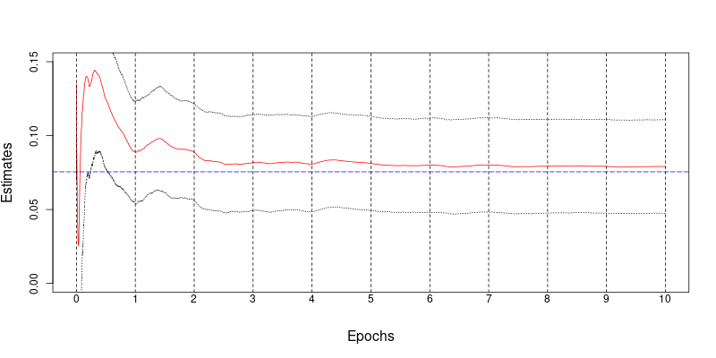
Figure 1. Estimation Path over Multiple Epochs in Angrist and Krueger (1991)

Notes. The solid line denotes the estimation path of SGMM PI over 10 epochs. The dotted line around the solid line represents the path of the corresponding 95% SGMM PI confidence intervals. The dashed horizontal line denotes the offline GMM estimate.

6.2. Angrist and Evans (1998)

In Angrist and Evans (1998), they study the effect of childbearing on female labor supply. In our application, we use data consisting of 394,840 observations from the 1980 U.S. census. The dependent variable is the number of working weeks divided by 52; the endogenous regressor is a binary variable that takes value 1 if the number of children is greater than 2; the instrument is a binary variable that takes value 1 if siblings are of the same sex. To be consistent between two applications, we repeat the same exercises as in the previous subsection. Specifically, we set $n_{0}=20,000$, $n=374,840$, and $n_{1}=10\sqrt{n}$. The initial-data-dependent choice $\gamma_{0}$ was that $\gamma_{0}=0.058$.

Table 4 and Figure 2 present the estimation results. As this is a just-identified case, we expect little difference across S2SLS and SGMM, which was empirically verified. It is interesting to notice that the SGMM estimate here basically converges only after one or two epochs, unlike the previous application. This is likely due to the fact that the number of parameters is just two, including the intercept term, and the model is just-identified in the second example.

Table 4. Estimation Results of Angrist and Evans (1998)

	Estimate of $\hat{\beta_{1}}$	95% CI	CI Length	Time (sec.)
2SLS	-0.1256	(-0.1714, -0.0797)	0.0917	$1.77$
GMM	-0.1256	(-0.1714, -0.0797)	0.0917	$1.92$
S2SLS	-0.1244	(-0.1921, -0.0567)	0.1354	$0.31$
SGMM RS	-0.1244	(-0.1921, -0.0567)	0.1354	$1.45$
SGMM PI	-0.1244	(-0.1770, -0.0717)	0.1053	$1.40$
SGMM ME	-0.1277	(-0.1759, -0.0796)	0.0963	$4.23$

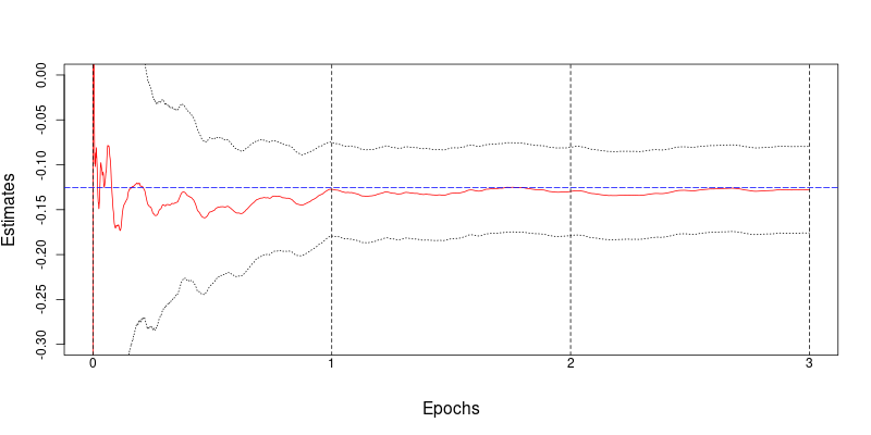
Figure 2. Estimation Path over Multiple Epochs in Angrist and Evans (1998)

Notes. Refer to the captions in Figure 1 for the corresponding legends.

7. Extensions

We conclude the paper by mentioning two possible extensions. First, recall the standard (nonlinear) GMM estimator for the general GMM model, $\mathbb{E}[g_{i}(\beta_{*})]=0$ with $\dim(g_{i})\geq d_{\beta}$:

(17) $$\min_{\beta}\bar{g}_{n}(\beta)^{\prime}W_{n}\bar{g}_{n}(\beta),$$

where $\bar{g}_{n}(\beta)=n^{-1}\sum_{i=1}^{n}g_{i}(\beta)$, and $W_{n}$ is a weighting matrix that may depend on an initial estimator of $\beta_{*}$. The first-order condition to (17) is

$$\frac{\partial}{\partial\beta}\bar{g}_{n}(\beta)^{\prime}W_{n}\bar{g}_{n}(\beta)=0.$$

The following is a natural efficient online algorithm for nonlinear GMM. We assume that the parameter space for $\beta$ is bounded in this case. For simplicity, we drop the step using the subsample of size $n_{1}$. Specifically, for $n_{0}$ as before, compute an initial estimate

(18a) $$\beta_{0} =\arg\min_{\beta}\bar{g}_{n_{0}}(\beta)^{\prime}\bar{g}_{n_{0}}(\beta)$$

(18b) $$\Phi_{0} =\frac{\partial}{\partial\beta}\bar{g}_{n_{0}}(\beta_{0})$$

(18c) $$W_{0} =\left(\frac{1}{n_{0}}\sum_{j=1}^{n_{0}}g_{j}(\beta_{0})g_{j}(\beta_{0})^{\prime}+\eta_{0}I\right)^{-1}.$$

Let $G_{i}(\beta)=\frac{\partial}{\partial\beta}g_{i}(\beta)$. We sequentially update from $i=1$ until $i=n$:

(19a) $$\beta_{i} =\beta_{i-1}-\gamma_{i}(\Phi_{i-1}^{\prime}W_{i-1}\Phi_{i-1})^{\dagger}\Phi_{i-1}^{\prime}W_{i-1}g_{i}(\beta_{i-1}),$$

(19b) $$\Phi_{i} =\Phi_{i-1}-\frac{1}{n_{0}+i}(\Phi_{i-1}-G_{i}(\bar{\beta}_{i-1})),$$

(19c) $$m_{i} =n_{0}+i-1+g_{i}(\bar{\beta}_{i-1})^{\prime}W_{i-1}g_{i}(\bar{\beta}_{i-1}),$$

(19d) $$W_{i} =\frac{n_{0}+i}{n_{0}+i-1}W_{i-1}\left[I-m_{i}^{-1}g_{i}(\bar{\beta}_{i-1})g_{i}(\bar{\beta}_{i-1})^{\prime}W_{i-1}\right],$$

(19e) $$\bar{\beta}_{i} =\bar{\beta}_{i-1}-\frac{1}{i}(\bar{\beta}_{i-1}-\beta_{i}).$$

We leave it to future research to derive the asymptotic properties of the above nonlinear SGMM. The online Sargan-Hansen test can be computed the same way as that in subsection 4.3.

Second, the instruments considered in the paper are assumed to be valid and strong. Allowing many weak IVs in general nonlinear GMM models is an important question that has been fruitfully studied in the past two decades. We expect that overidentified Z-type stochastic approximation is appealing with many weak IVs because it can be helpful to deal with the problem of many local minima. For instance, being a fast algorithm, overidentified Z-type stochastic approximation gives us an avenue of attempting many different starting values. However, we expect that the theoretical studies could be technically challenging, so we leave this extension for future research.

Appendix A Appendix

A.1. Proofs

Throughout the proofs, with no loss of generality, assume $\beta_{*}=0$ so that $\mathbb{E}[H_{i}]=0$, under iid assumption $\mathbb{E}[H_{i}\mid\mathcal{F}_{i-1}]=0$ and $\mathbb{E}[g_{i}(\beta_{i-1})\mid\mathcal{F}_{i-1}]=G\beta_{i-1}$.

A generic positive constant will be denoted by $K>0$, whose value may differ in each occurrence. For future reference, for each $R>0$, we consider the stopping times defined as follows.

(20) $$\begin{array}[]{rl}\tau_{R}&=\inf\{i\geq 0:\|\beta_{i}\|\geq R\},\\[6.0pt] \sigma_{R}&=\inf\{i\geq 0:\max\{\|W_{i}\|,\|(\Phi_{i-1}^{\prime}W_{i-1}\Phi_{i-1})^{\dagger}\|\}\geq R\},\\[6.0pt] \rho_{R}&=\inf\{i\geq 0:\|\Phi_{i}-G\|/\eta_{i+1}\geq R\},\\[6.0pt] \iota_{R}&=\inf\{i\geq 0:\|(\Phi_{i}^{\prime}\Phi_{i})^{\dagger}\|\geq R\},\end{array}$$

where $\eta_{i}=i^{-1/2}\log_{+}\log_{+}(i)^{1/2}$ for $\log_{+}(x):=\max\{\log x,1\}$. We regard $\inf\varnothing=\infty$.

Proof of Lemma 1.

Let us denote $B_{i}:=\|\beta_{i}\|^{2}$. Expanding the square $\|\beta_{i}\|^{2}=\|\beta_{i-1}-\gamma_{i}(\Phi_{i-1}^{\prime}W_{i-1}\Phi_{i-1})^{\dagger}\Phi_{i-1}^{\prime}W_{i-1}g_{i}(\beta_{i-1})\|^{2}$, we have

(21) $$B_{i} =B_{i-1}-2\gamma_{i}\beta_{i-1}^{\prime}(\Phi_{i-1}^{\prime}W_{i-1}\Phi_{i-1})^{\dagger}\Phi_{i-1}^{\prime}W_{i-1}g_{i}(\beta_{i-1})$$

$$\qquad+\gamma_{i}^{2}g_{i}(\beta_{i-1})^{\prime}W_{i-1}\Phi_{i-1}(\Phi_{i-1}^{\prime}W_{i-1}\Phi_{i-1})^{\dagger}{}^{2}\Phi_{i-1}^{\prime}W_{i-1}g_{i}(\beta_{i-1}).$$

Taking a conditional expectation $\mathbb{E}[\cdot\mid\mathcal{F}_{i-1}]$ on both sides, the second term on the right-hand side of (21) yields $-2\gamma_{i}\beta_{i-1}^{\prime}(\Phi_{i-1}^{\prime}W_{i-1}\Phi_{i-1})^{\dagger}\Phi_{i-1}^{\prime}W_{i-1}G\beta_{i-1}$. For the third term, since we have

$$\left\|{(\Phi_{i-1}^{\prime}W_{i-1}\Phi_{i-1})^{\dagger}\Phi_{i-1}^{\prime}W_{i-1}^{1/2}}\right\|^{2} =\left\|{W_{i-1}^{1/2}\Phi_{i-1}(\Phi_{i-1}^{\prime}W_{i-1}\Phi_{i-1})^{\dagger}{}^{2}\Phi_{i-1}^{\prime}W_{i-1}^{1/2}}\right\|$$

$$=\left\|{(\Phi_{i-1}^{\prime}W_{i-1}\Phi_{i-1})^{\dagger}}\right\|,$$

it follows that

$$\mathbb{E}[g_{i}(\beta_{i-1})^{\prime}W_{i-1}\Phi_{i-1}(\Phi_{i-1}^{\prime}W_{i-1}\Phi_{i-1})^{\dagger}{}^{2}\Phi_{i-1}^{\prime}W_{i-1}g_{i}(\beta_{i-1})\mid\mathcal{F}_{i-1}]$$

$$\leq 2\mathbb{E}[\beta_{i-1}^{\prime}G_{i}^{\prime}W_{i-1}\Phi_{i-1}(\Phi_{i-1}^{\prime}W_{i-1}\Phi_{i-1})^{\dagger}{}^{2}\Phi_{i-1}^{\prime}W_{i-1}G_{i}\beta_{i-1}$$

$$\qquad+H_{i}^{\prime}W_{i-1}\Phi_{i-1}(\Phi_{i-1}^{\prime}W_{i-1}\Phi_{i-1})^{\dagger}{}^{2}\Phi_{i-1}^{\prime}W_{i-1}H_{i}\mid\mathcal{F}_{i-1}]$$

$$\lesssim\left\|{W_{i-1}}\right\|\left\|{(\Phi_{i-1}^{\prime}W_{i-1}\Phi_{i-1})^{\dagger}}\right\|\mathbb{E}[\|\beta_{i-1}\|^{2}\left\|{G_{i}}\right\|^{2}+\|H_{i}\|^{2}\mid\mathcal{F}_{i-1}]$$

$$\lesssim\left\|{W_{i-1}}\right\|\left\|{(\Phi_{i-1}^{\prime}W_{i-1}\Phi_{i-1})^{\dagger}}\right\|(B_{i-1}+1)$$

where the second-to-last inequality uses Assumptions 1 and 6. As a result,

(22) $$\mathbb{E}[B_{i}\mid\mathcal{F}_{i-1}] \leq B_{i-1}-2\gamma_{i}\beta_{i-1}^{\prime}(\Phi_{i-1}^{\prime}W_{i-1}\Phi_{i-1})^{\dagger}\Phi_{i-1}^{\prime}W_{i-1}G\beta_{i-1}$$

$$\quad+K\gamma_{i}^{2}\|{W_{i-1}}\|\|(\Phi_{i-1}^{\prime}W_{i-1}\Phi_{i-1})^{\dagger}\|(B_{i-1}+1).$$

for some $K>0$. Note that

(23) $$-\beta_{i-1}^{\prime}(\Phi_{i-1}^{\prime}W_{i-1}\Phi_{i-1})^{\dagger}\Phi_{i-1}^{\prime}W_{i-1}G\beta_{i-1}$$

$$= -\beta_{i-1}^{\prime}(\Phi_{i-1}^{\prime}W_{i-1}\Phi_{i-1})^{\dagger}\Phi_{i-1}^{\prime}W_{i-1}\Phi_{i-1}\beta_{i-1}+\beta_{i-1}^{\prime}(\Phi_{i-1}^{\prime}W_{i-1}\Phi_{i-1})^{\dagger}\Phi_{i-1}^{\prime}W_{i-1}(\Phi_{i-1}-G)\beta_{i-1}$$

$$\leq -\beta_{i-1}^{\prime}(\Phi_{i-1}^{\prime}W_{i-1}\Phi_{i-1})^{\dagger}\Phi_{i-1}^{\prime}W_{i-1}\Phi_{i-1}\beta_{i-1}+\|\beta_{i-1}\|^{2}\|(\Phi_{i-1}^{\prime}W_{i-1}\Phi_{i-1})^{\dagger}\|^{1/2}\|W_{i-1}\|^{1/2}\|\Phi_{i-1}-G\|.$$

Note that there exists $\delta>0$ such that if $\|\Phi_{i-1}-G\|<\delta$ holds true, then the inverse matrix $(\Phi_{i-1}^{\prime}W_{i-1}\Phi_{i-1})^{\dagger}=(\Phi_{i-1}^{\prime}W_{i-1}\Phi_{i-1})^{-1}$ exists. As a result, on this event $\{\|\Phi_{i-1}-G\|<\delta\}$, it holds

$$-\beta_{i-1}^{\prime}(\Phi_{i-1}^{\prime}W_{i-1}\Phi_{i-1})^{\dagger}\Phi_{i-1}^{\prime}W_{i-1}G\beta_{i-1}$$

$$\leq -\|\beta_{i-1}\|^{2}+\|\beta_{i-1}\|^{2}\|(\Phi_{i-1}^{\prime}W_{i-1}\Phi_{i-1})^{\dagger}\|^{1/2}\|W_{i-1}\|^{1/2}\|\Phi_{i-1}-G\|;$$

whereas on the event $\{\|\Phi_{i-1}-G\|\geq\delta\}$, (23) implies trivially that

$$-\beta_{i-1}^{\prime}(\Phi_{i-1}^{\prime}W_{i-1}\Phi_{i-1})^{\dagger}\Phi_{i-1}^{\prime}W_{i-1}G\beta_{i-1}$$

$$\leq \ \|\beta_{i-1}\|^{2}\|(\Phi_{i-1}^{\prime}W_{i-1}\Phi_{i-1})^{\dagger}\|^{1/2}\|W_{i-1}\|^{1/2}\|\Phi_{i-1}-G\|.$$

Putting this together with (22), it follows

(24) $$\mathbb{E}[B_{i}\mid\mathcal{F}_{i-1}]$$

$$\leq \ B_{i-1}\big{(}1+2\gamma_{i}\|\Phi_{i-1}-G\|\|W_{i-1}\|^{1/2}\|(\Phi_{i-1}^{\prime}W_{i-1}\Phi_{i-1})^{\dagger}\|^{1/2}+K\gamma_{i}^{2}\|W_{i-1}\|\|(\Phi_{i-1}^{\prime}W_{i-1}\Phi_{i-1})^{\dagger}\|\big{)}$$

$$+K\gamma_{i}^{2}\|W_{i-1}\|\|(\Phi_{i-1}^{\prime}W_{i-1}\Phi_{i-1})^{\dagger}\|-2\gamma_{i}B_{i-1}1\{\|\Phi_{i-1}-G\|<\delta\}$$

for some $K>0$, where $1_{A}$ denotes an indicator function for a set $A$.

By Assumption 6 and the law of iterated logarithm (LIL), $\limsup_{i\to\infty}{\|\Phi_{i-1}-G\|}/{\eta_{i}}\leq c$ holds almost surely for some $c>0$, which implies that $1\{\|\Phi_{i-1}-G\|<\delta\}=1$ holds for all but finitely many $i$ almost surely. Also, using the fact that $\lim_{i\to\infty}W_{i-1}=W$ and $\lim_{i\to\infty}(\Phi_{i-1}^{\prime}W_{i-1}\Phi_{i-1})^{\dagger}=(G^{\prime}WG)^{-1}$ by the strong law of large numbers (SLLN), we have

$$\sum_{i=1}^{\infty}(2\gamma_{i}\|\Phi_{i-1}-G\|\|W_{i-1}\|^{1/2}\|(\Phi_{i-1}^{\prime}W_{i-1}\Phi_{i-1})^{\dagger}\|^{1/2}+K\gamma_{i}^{2}\|W_{i-1}\|\|(\Phi_{i-1}^{\prime}W_{i-1}\Phi_{i-1})^{\dagger}\|)<\infty$$

almost surely (a.s.)

By Lemma 2, it follows that $\lim_{i\to\infty}B_{i}=B_{\infty}<\infty$ and $\sum_{i=1}^{\infty}\gamma_{i}B_{i-1}1\{\|\Phi_{i-1}-G\|<\delta\}<\infty$ exist a.s. This implies that $B_{\infty}=0$ a.s., because otherwise $\sum_{i}\gamma_{i}<\infty$, which is in contradiction to Assumption that $\gamma_{i}=\gamma_{0}i^{-a}$ with $a\in(1/2,1]$. Therefore, $\lim_{n\to\infty}\|\beta_{n}\|=0$ a.s., and we conclude that $\beta_{n}\to\beta_{*}$ as $n\to\infty$ a.s.. ∎

Proof of Theorem 1.

Part 1. Local $L^{2}$-convergence rate.

Consider the stopping time $T_{R}=\min\{\sigma_{R},\rho_{R}\}$ defined as per (20). In Part 1, we aim to establish the convergence rate of $\mathbb{E}[\|\beta_{i}\|^{2}1\{T_{R}\geq i\}]$ to 0. The proof stems from (24) with the fact that the event $T_{R}\geq i$ implies $\|W_{i-1}\|\leq R$, $\|(\Phi_{i-1}^{\prime}W_{i-1}\Phi_{i-1})^{\dagger}\|\leq R$, and $\|\Phi_{i-1}-G\|\leq R\eta_{i}$.

Note that $\sup_{i\geq 0}\|W_{i}\|<\infty$ and $\sup_{i\geq 0}\|(\Phi_{i}^{\prime}W_{i}\Phi_{i})^{\dagger}\|<\infty$ holds a.s. by the SLLN, and also that $\sup_{i\geq 0}\|\Phi_{i}-G\|/\eta_{i+1}<\infty$ a.s. by the LIL. Thus, it follows $\mathbb{P}(T_{R}=\infty\text{ for some }R>0)=1$. From (24) in the proof of Lemma 1, we can see that on $\{T_{R}\geq i\}$, it holds

$$\|\Phi_{i-1}-G\|\|W_{i-1}\|^{1/2}\|(\Phi_{i-1}^{\prime}W_{i-1}\Phi_{i-1})^{\dagger}\|^{1/2}\leq R^{2}\eta_{i}.$$

Thus, for all sufficiently large $i$ such that $\eta_{i}\leq\frac{1}{2R^{2}}$, it holds

(25) $$\mathbb{E}[B_{i}1\{T_{R}\geq i\}\mid\mathcal{F}_{i-1}]\leq B_{i-1}1\{T_{R}\geq i-1\}(1-\alpha\gamma_{i}+K\gamma_{i}^{2})+K\gamma_{i}^{2}$$

for some $\alpha>0$. By integrating both sides of this inequality, we obtain

$$\mathbb{E}[B_{i}1\{T_{R}>i\}]\leq\mathbb{E}[B_{i-1}1\{T_{R}>i-1\}](1-\alpha\gamma_{i}+K\gamma_{i}^{2})+K\gamma_{i}^{2}.$$

By Lemma 3, it follows that $\mathbb{E}[B_{i}1\{T_{R}>i\}]=O(\gamma_{i})$ for any choice of $R>0$.

Part 2. Coupling with the linearized process $\beta_{i}^{1}$.

Define an auxiliary process $\beta_{i}^{1}$ as follows.

(26) $$\beta_{i}^{1}:=(1-\gamma_{i})\beta_{i-1}^{1}-\gamma_{i}\xi_{i}$$

where $\beta_{0}^{1}:=\beta_{0}$, $\tilde{G}_{i}:=G_{i}-G$ and

(27) $$\xi_{i}:=(\Phi_{i-1}^{\prime}W_{i-1}\Phi_{i-1})^{\dagger}\Phi_{i-1}^{\prime}W_{i-1}(\tilde{G}_{i}\beta_{i-1}+H_{i}).$$

Also define $\bar{\beta}_{i}^{1}=\frac{1}{i}\sum_{j=1}^{i}\beta_{j}^{1}$ analogously to $\bar{\beta}_{i}$.

Define $\delta_{i}=\beta_{i}-\beta_{i}^{1}$ as the difference between $\beta_{i}$ and its approximation $\beta_{i}^{1}$. By Lemma 5, it follows that $\sqrt{n}(\bar{\beta}_{1}-\bar{\beta}_{n}^{1})=\frac{1}{\sqrt{n}}\sum_{i=1}^{n}\delta_{i}=o_{P}(1)$, wherein we used the local convergence rate established in Part 1. Hence, we have $\sqrt{n}\bar{\beta}_{n}=\sqrt{n}\bar{\beta}_{n}^{1}+o_{P}(1)$.

Part 3. We now assert that the sequence $\beta_{i}^{1}$ is the SGD sequence of Polyak and Juditsky’s (1992, PJ hereafter) Theorem 1-(a) by verifying its Assumptions 2.1 to 2.5-(a). First of all, the “true parameter” for this sequence is zero because we have assumed $\beta_{*}=0$. Assumption 2.1 is straightforward to check because $A=I$ in our case. Secondly, $\xi_{i}$ defined in (27) is a martingale difference sequence (mds) because $\mathbb{E}[H_{i}\mid\mathcal{F}_{i-1}]=H=-G\beta_{*}=0$ and

$$\mathbb{E}[\xi_{i}\mid\mathcal{F}_{i-1}]=\Phi_{i-1}^{\prime}W_{i-1}(\mathbb{E}[\tilde{G}_{i}\mid\mathcal{F}_{i-1}]\beta_{i-1}+H)=0.$$

This deals with Assumption 2.2. In addition, Assumptions 2.3-2.5(a) of PJ are verified in Lemma 4. It then follows from Theorem 1-(a) in Polyak and Juditsky (1992) that $\sqrt{n}\bar{\beta}_{n}^{1}\overset{d}{\to}N(0,(G^{\prime}WG)^{-1}G^{\prime}W\Omega WG(G^{\prime}WG)^{-1})$. We conclude $\sqrt{n}\bar{\beta}_{n}\overset{d}{\to}N(0,(G^{\prime}WG)^{-1}G^{\prime}W\Omega WG(G^{\prime}WG)^{-1})$.

∎

Proof of Theorem 2.

We maintain the assumption $\beta_{*}=0$. Let us define

(28) $$\bar{\nu}(r) =\frac{1}{\sqrt{n}}\sum_{i=0}^{\lfloor nr\rfloor}\beta_{i},$$

$$\bar{\nu}^{1}(r) =\frac{1}{\sqrt{n}}\sum_{i=0}^{\lfloor nr\rfloor}\beta^{1}_{i},$$

for $r\in[0,1]$ and $\beta^{1}$ as defined in the proof of Theorem 1. By Lemma 5, we have that $\sup_{r\in[0,1]}\|\bar{\nu}(r)-\bar{\nu}^{1}(r)\|=\frac{1}{\sqrt{n}}\sup_{1\leq m\leq n}\left\|\sum_{i=1}^{m}(\beta_{i}-\beta_{i}^{1})\right\|=o_{P}(1)$. This allows us to prove Theorem 2 with $\bar{\nu}^{1}(r)$ in lieu of $\bar{\nu}(r)$.

Now, we consider a decomposition $\bar{\nu}^{1}(r)=I_{1}(r)-I_{2}(r)-I_{3}(r)$, defined as

$$I_{1}(r) =\frac{1}{\sqrt{n}\gamma_{0}}\alpha_{0}^{\lfloor nr\rfloor}\beta_{0},$$

$$I_{2}(r) =\frac{1}{\sqrt{n}}\sum_{i=1}^{\lfloor nr\rfloor}\xi_{i},$$

$$I_{3}(r) =\frac{1}{\sqrt{n}}\sum_{i=1}^{\lfloor nr\rfloor}w^{\lfloor nr\rfloor}_{i}\xi_{i},$$

with $\xi_{i}$ defined in (27), $\alpha_{j}^{n}:=\gamma_{j}\sum_{i=j}^{n}\prod_{k=j+1}^{i}(1-\gamma_{k})$ and $w_{j}^{m}:=\alpha_{j}^{m}-1$. Observe that $|\alpha_{j}^{n}|\lesssim 1$ holds uniformly for all $j\leq n$ by Lemma 1-(ii) in Polyak and Juditsky (1992), and hence $|w_{j}^{m}|\lesssim 1$ also holds uniformly. Moreover, we have $\sum_{j=1}^{m}|w_{j}^{m}|=O(m^{a})$ (Zhu and Dong, 2021).

Since $\alpha_{0}^{m}$ is uniformly bounded in $m$, it is easy to see that $\sup_{r}\|I_{1}(r)\|=o_{P}(1)$. For $I_{2}(r)$, a standard FCLT for mds applies and yields $\{I_{2}(r)\}_{r\in[0,1]}\rightsquigarrow\operatorname{Avar}(\bar{\beta})^{1/2}\{W_{d_{\beta}}(r)\}_{r\in[0,1]}$. Note that sufficient conditions for FCLT are provided by Lemma 4.

For the third term, we split $I_{3}(r)$ into two components:

$$I_{3}(r) =\frac{1}{\sqrt{n}}\sum_{i=1}^{\lfloor nr\rfloor}w^{\lfloor nr\rfloor}_{i}(\Phi_{i-1}^{\prime}W_{i-1}\Phi_{i-1})^{\dagger}\Phi_{i-1}^{\prime}W_{i-1}\tilde{G}_{i}\beta_{i-1}$$

$$\quad+\frac{1}{\sqrt{n}}\sum_{i=1}^{\lfloor nr\rfloor}w^{\lfloor nr\rfloor}_{i}(\Phi_{i-1}^{\prime}W_{i-1}\Phi_{i-1})^{\dagger}\Phi_{i-1}^{\prime}W_{i-1}H_{i}$$

$$=:I_{31}(r)+I_{32}(r).$$

Under Assumption 7, the treatment of $\sup_{r}\|I_{32}(r)\|=o_{P}(1)$ can be approached in a similar manner to that in Lee et al. (2022a) for their linear least squares regression, which will be omitted here. However, the term $I_{31}(r)$ cannot be handled in the same manner due to the absence of ex-ante moment conditions for $\beta_{i-1}$. To reach a proper bound for $\beta_{i-1}$, we consider $T_{R}=\min\{\tau_{R},\sigma_{R}\}$. Then on the event $\{T_{R}\geq i\}$, we have $\|\beta_{i-1}\|\leq{R}$, $\|(\Phi_{i-1}^{\prime}W_{i-1}\Phi_{i-1})^{\dagger}\|\leq R$ and $\|W_{i-1}\|\leq R$.

Let us denote $S_{m}:=\sum_{i=1}^{m}w_{i}^{m}(\Phi_{i-1}^{\prime}W_{i-1}\Phi_{i-1})^{\dagger}\Phi_{i-1}^{\prime}W_{i-1}\tilde{G}_{i}\beta_{i-1}$ and $S_{m\wedge T_{R}}:=S_{\min\{m,T_{R}\}}$ for $m\geq 1$. We examine the first component of $I_{3}(r)$, which satisfies

$$\sup_{r\in[0,1]}\|I_{31}(r)\|=n^{-1/2}\sup_{1\leq m\leq n}\|S_{m}\|.$$

Let $p$ be an integer such that $p>(1-a)^{-1}$ (see Assumption 7). Note that on the event $\{T_{R}>n\}$, it holds

$$\sup_{1\leq m\leq n}\|S_{m}\|^{2p}\leq\sum_{m=1}^{n}\|S_{m}\|^{2p}=\sum_{m=1}^{n}\|S_{m\wedge T_{R}}\|^{2p}$$

From this, we have

$$\mathbb{E}[\sup_{r}\|I_{31}(r)\|^{2p}1\{T_{R}>n\}]\leq n^{-p}\sum_{m=1}^{n}\mathbb{E}[\|S_{m\wedge T_{R}}\|^{2p}].$$

Write $A_{i}:=(\Phi_{i-1}^{\prime}W_{i-1}\Phi_{i-1})^{\dagger}\Phi_{i-1}^{\prime}W_{i-1}\tilde{G}_{i}\beta_{i-1}1\{T_{R}\geq i\}$. Note that $\{T_{R}\geq i\}$ is equivalent to $\{\max_{j\leq i-1}\{\|\beta_{j}\|,\|(\Phi_{j}^{\prime}W_{j}\Phi_{j})^{-1}\|,\|W_{j}\|\}<R\}$, which belongs to $\mathcal{F}_{i-1}$. Hence, $w_{i}^{m}A_{i}$ constitutes a mds, and we can express $S_{m\wedge T_{R}}$ as follows:

$$S_{m\wedge T_{R}}=\sum_{i=1}^{m}w_{i}^{m}(\Phi_{i-1}^{\prime}W_{i-1}\Phi_{i-1})^{\dagger}\Phi_{i-1}^{\prime}W_{i-1}\tilde{G}_{i}\beta_{i-1}1\{T_{R}\geq i\}=\sum_{i=1}^{m}w_{i}^{m}A_{i}.$$

Also note that $\|A_{i}\|\leq R^{2}\|\tilde{G}_{i}\|$. Applying Burkholder’s inequality (e.g., Hall and Heyde, 1980) to $\|\sum_{i=1}^{m}w_{i}^{m}A_{i}\|^{2p}$, we get

$$\mathbb{E}[\sup_{r}\|I_{31}(r)\|^{2p}1\{T_{R}>n\}]$$

$$\leq \ n^{-p}\sum_{m=1}^{n}\mathbb{E}[\|S_{m\wedge T_{R}}\|^{2p}]=\ n^{-p}\sum_{m=1}^{n}\mathbb{E}[\|\sum_{i=1}^{m}w_{i}^{m}A_{i}\|^{2p}]$$

$$\leq \ n^{-p}\sum_{m=1}^{n}\mathbb{E}\left(\sum_{i=1}^{m}\|w_{i}^{m}A_{i}\|^{2}\right)^{p}$$

$$\leq \ n^{-p}\sum_{m=1}^{n}\sum_{i_{1},...,i_{p}}^{m}|w_{i_{1}}^{m}|^{2}...|w_{i_{p}}^{m}|^{2}\mathbb{E}\|A_{i_{1}}\|^{2}...\|A_{i_{p}}\|^{2}$$

$$\leq \ n^{-p}\sum_{m=1}^{n}\sum_{i_{1},...,i_{p}}^{m}|w_{i_{1}}^{m}|^{2}...|w_{i_{p}}^{m}|^{2}\max_{j\leq m}\mathbb{E}\|A_{j}\|^{2p}\cdot p$$

$$\lesssim \ n^{-p}\sum_{m=1}^{n}\left(\sum_{i=1}^{m}|w^{m}_{i}|\right)^{p}\lesssim\ n^{-p}\sum_{m=1}^{n}m^{ap}\lesssim n^{-(1-a)p+1}\to 0$$

where Young’s inequality $\prod_{r=1}^{p}\|a_{r}\|\lesssim\sum_{r=1}^{p}\|a_{r}\|^{p}$ is invoked for deriving the second-to-last line. Hence, $\sup_{r}\|I_{31}(r)\|1\{T_{R}>n\}=o_{P}(1)$ as $n\to\infty$. By the same argument as used in the proof of Lemma 5, we have $\sup_{r}\|I_{31}(r)\|\to_{p}0$. We conclude $\{\bar{\nu}(r)\}_{r\in[0,1]}\rightsquigarrow\operatorname{Avar}(\bar{\beta})^{1/2}\{W_{d_{\beta}}(r)\}_{r\in[0,1]}.$ ∎

Proof of Theorem 3.

The proof of Theorem 3 differs from that of Theorem 1 under the fully online setting as there is a need to deal with the triangular array $(W_{i,n})_{i=0}^{n-1}$ of weighting matrices, as defined in (5d). It is worth noting that this introduces a dependence of $(\beta_{i,n})_{i=1}^{n}$ on $n$, emerging due to the varying size $n_{1}=n_{1}(n)$ of $\mathbb{S}_{1}$ as the sample size $n$ changes. Since $n_{1}$ may vary with $n$, it is possible to have $W_{i,n}\neq W_{i,m}$ for $n\neq m$, posing a challenge when analyzing the behavior of $(W_{i,n})_{i=0}^{n-1}$ using previous approaches. As a result, an alternative technique is employed to handle the triangular array structure in this proof.

Part 1. $L^{2}$-convergence rate and consistency of SGD from the efficient algorithm (5a)–(5e).

We will first derive the uniform $L^{2}$-convergence rate for the class of all admissible weighting schemes $(W_{i})_{i=0}^{n-1}$. To this end, we allow $W_{i}$ to be a possibly random positive definite matrix adapted to the filtration $\mathcal{F}_{i}$. For instance, in the updating rule in (2d), $W_{i}$ is treated as a unit point mass at $\frac{i}{i-1}(W_{i-1}-\frac{1}{m_{i}}W_{i-1}z_{i}z_{i}^{\prime}W_{i-1}),$ which is $\mathcal{F}_{i}$-measurable. Note that admissible weighting schemes allow for a broader range of possibilities than the proposed updating rule.

We denote $W_{[n]}$ as the sequence of weighting matrices $(W_{i})_{i=0}^{n-1}$ up to $n-1$ and say that $W_{[n]}\in\mathcal{A}$ if $W_{[n]}$ is an admissible weighting scheme. To differentiate the proposed updating scheme from a generic one, we denote $W_{i,n}$ as the weighting matrix following the rule (5d) with $n_{1}(n)$ as the change-point. For $C\geq 1$, define an event $\{W_{[k]}\in\mathcal{E}(C)\}\in\mathcal{F}_{k-1}$ as

$$\{W_{[k]}\in\mathcal{E}(C)\}=\{1/C\leq\lambda_{\min}(W_{j})\leq\lambda_{\max}(W_{j})\leq C,\ j=1,\ldots,k-1\}.$$

For given $R>0$ and $C\geq 1$, we consider the sequence

$$d_{i}:=\sup_{W_{[i]}\in\mathcal{A}}\mathbb{E}[\|\beta_{i}\|^{2}1\{T_{R}\geq i,W_{[i]}\in\mathcal{E}(C)\}].$$

where $T_{R}:=\min\{\rho_{R},\iota_{R}\}$ and the supremum is taken over all admissible weighting schemes. Note that $d_{0}<\infty$ is well-defined because $\mathbb{E}[\|\beta_{0}\|^{2}]<\infty$. By the inductive step below, we can also see that $d_{i}<\infty$ for all $i\geq 0$. We aim to establish $d_{n}=O(\gamma_{n})$. Note that on an event $\{T_{R}\geq i,W_{[i]}\in\mathcal{E}(C)\}\in\mathcal{F}_{i-1}$ where $W_{[i]}\in\mathcal{A}$, it follows from (24) that

$$\mathbb{E}[\|\beta_{i}\|^{2}\mid\mathcal{F}_{i-1}] \leq\|\beta_{i-1}\|^{2}(1-\gamma_{i}/2+K\gamma_{i}^{2})+K\gamma_{i}^{2}$$

for all sufficiently large $i$. Since $\{T_{R}\geq i,W_{[i]}\in\mathcal{E}(C)\}\subseteq\{T_{R}\geq i-1,W_{[i-1]}\in\mathcal{E}(C)\}$, we obtain

$$\mathbb{E}[\|\beta_{i}\|^{2}1\{T_{R}\geq i,W_{[i]}\in\mathcal{E}(C)\}]$$

$$\leq \ \mathbb{E}[\|\beta_{i-1}\|^{2}1\{T_{R}\geq i-1,W_{[i-1]}\in\mathcal{E}(C)\}](1-\gamma_{i}/2+K\gamma_{i}^{2})+K\gamma_{i}^{2},$$

whence it follows

$$d_{i}\leq d_{i-1}(1-\gamma_{i}/2+K\gamma_{i}^{2})+K\gamma_{i}^{2}$$

for all sufficiently large $i$ by taking supremum over $W_{[i]}$ on both sides. By Lemma 3, it follows $d_{n}=O(\gamma_{n})$ as $n\to\infty$.

By specializing this to $W_{[n],n}$, which is trivially admissible, we obtain

$$\mathbb{E}[\|\beta_{n}\|^{2}1\{T_{R}\geq n,W_{[n],n}\in\mathcal{E}(C)\}]\leq O(\gamma_{n})\to 0$$

and

$$\mathbb{E}\left[\left\|\frac{1}{n}\sum_{i=1}^{n}\beta_{i}1\{T_{R}\geq i,W_{[i],n}\in\mathcal{E}(C)\}\right\|^{2}\right]\to 0.$$

Note that, thus far, the convergence is uniform in the choice of the change-point $n_{1}$ for any given $R$ and $C$.

Next, our goal is to establish that $\beta_{n,n}=o_{P}(1)$ and $\bar{\beta}_{n,n}=o_{P}(1)$ when $n_{1}$ is chosen such that $n_{1}\to\infty$ as $n\to\infty$. We drop the duplicate $n$ in the subscripts and denote them just by $\beta_{n}$ and $\bar{\beta}_{n}$ for brevity of notation. Accordingly, $W_{i,n}$ will also be denoted as $W_{i}$ occasionally for notational ease.

Given that $n_{1}$ is chosen such that $n_{1}(n)\to\infty$, we verify that it holds

(29) $$\lim_{C\to\infty}\liminf_{n\to\infty}\mathbb{P}(W_{[n],n}\in\mathcal{E}(C))=1,$$

i.e., $\mathbb{P}(W_{[n],n}\in\mathcal{E}(C))$ can be made arbitrarily close to 1 uniformly in $n$ for a sufficiently large $C$. Once this is verified, coupled with the fact that $\sup_{n\in\mathbb{N}}\mathbb{P}(T_{R}\leq n)=\mathbb{P}(T_{R}<\infty)<\varepsilon$ for sufficiently large $R>0$, it implies that

$$\mathbb{P}(\|\beta_{n}-\beta_{n}1\{T_{R}\geq n,W_{[n],n}\in\mathcal{E}(C)\}\|>\varepsilon)<2\varepsilon,$$

and

$$\mathbb{P}\left(\left\|\bar{\beta}_{n}-\frac{1}{n}\sum_{i=1}^{n}\beta_{i}1\{T_{R}\geq i,W_{[i],n}\in\mathcal{E}(C)\}\right\|>\varepsilon\right)<2\varepsilon,$$

which establishes $\beta_{n}=\beta_{n}1\{T_{R}>n,W_{[n],n}\in\mathcal{E}(C)\}+o_{P}(1)=o_{P}(1)$ and $\bar{\beta}_{n}=o_{P}(1)$.

We start with a convenient observation. Define $W^{*}_{i}:=W_{i,n}$ for $n$ such that $i\leq n_{1}(n)$. Note that there is no ambiguity in this definition since $W_{i,n}=W_{i,m}$ whenever $n_{1}(n)\geq i$ and $n_{1}(m)\geq i$ hold. This is well-defined as we assumed $n_{1}\to\infty$ and hence $W_{i}^{*}=\lim_{n}W_{i,n}$ holds. Since $W^{*}_{r}=(\frac{n_{0}}{n_{0}+r}W_{0}^{-1}+\frac{1}{n_{0}+r}\sum_{j=1}^{r}z_{j}z_{j}^{\prime})^{-1}$, $r\geq 1$ converges a.s. to a positive definite matrix $Q^{-1}$ as $r\to\infty$ by the SLLN, we can see that with probability 1, $(\lambda_{\min}(W^{*}_{i}))_{i=1}^{\infty}$ is bounded away from 0 and $(\lambda_{\max}(W^{*}_{i}))_{i=1}^{\infty}$ is bounded from above. This implies that

$$\lim_{C\to\infty}\liminf_{n\to\infty}\mathbb{P}(C^{-1}\leq\lambda_{\min}(W_{j,n})\leq\lambda_{\max}(W_{j,n})\leq C,j=0,\ldots,n_{1})$$

$$\geq \ \lim_{C\to\infty}\mathbb{P}(C^{-1}\leq\lambda_{\min}(W_{j}^{*})\leq\lambda_{\max}(W_{j}^{*})\leq C,j=0,1,\ldots)=1.$$

This observation allows us to establish only

(30) $$\lim_{C\to\infty}\liminf_{n\to\infty}\mathbb{P}(C^{-1}\leq\lambda_{\min}(W_{j,n})\leq\lambda_{\max}(W_{j,n})\leq C,n_{1}<j\leq n)=1$$

to prove (29).

Furthermore, it is useful to note that, for $\beta^{*}_{i}:=\beta_{i,n}$ and $\bar{\beta}^{*}_{i}:=\bar{\beta}_{i,n}$ defined in a similar manner to that of $W_{i}^{*}$, we have $\beta^{*}_{r}\to 0$ and $\bar{\beta}^{*}_{r}\to 0$ as $r$ tends to infinity by Lemma 1. In particular, this implies the strong consistency of $\bar{\beta}_{n_{1}}=\bar{\beta}_{n_{1}}^{*}$ as $n\to\infty$, which will be utilized in the subsequent analysis.

To verify (30), note that

$$\mathbb{P}(C^{-1}\leq\lambda_{\min}(W_{j,n})\leq\lambda_{\max}(W_{j,n})\leq C,j=n_{1}+1,\ldots,n)$$

$$= \ \mathbb{P}\left(\left\{C^{-1}\leq\min_{n_{1}<j\leq n}\lambda_{\min}(W_{j,n}^{-1})\right\}{\textstyle\bigcap}\left\{\max_{n_{1}<j\leq n}\lambda_{\max}(W_{j,n}^{-1})\leq C\right\}\right)$$

$$\geq \ \mathbb{P}\left(C^{-1}\leq\min_{n_{1}<j\leq n}\lambda_{\min}(W_{j,n}^{-1})\right)+\mathbb{P}\left(\max_{n_{1}<j\leq n}\lambda_{\max}(W_{j,n}^{-1})\leq C\right)-1$$

$$=: \ P_{1}(C)+P_{2}(C)-1.$$

We will show that $\lim_{C\to\infty}\liminf_{n\to\infty}P_{j}(C)=1$ for each $j=1,2$, which then establishes (30).

We first address $P_{1}(C)$. For brevity of notation, let us denote $\mathbb{E}_{m:n}[X_{j}]=\frac{1}{n-m}\sum_{j=m+1}^{n}X_{j}$ as the empirical average of $X_{j}$ from $j=m+1$ to $n$. We observe that

$$W_{i,n}^{-1}=\frac{n_{0}+n_{1}}{n_{0}+n_{1}+k}W_{n_{1}}^{-1}+\frac{k}{n_{0}+n_{1}+k}\mathbb{E}_{n_{1}:n_{1}+k}[g_{j}(\bar{\beta}_{n_{1}})g_{j}(\bar{\beta}_{n_{1}})^{\prime}]$$

where $k:=i-n_{1}\in\{1,\ldots,n_{2}\}$ and $n_{2}:=n-n_{1}(n)$. Thus, each $W_{i,n}^{-1}$ is given by a weighted average of $W_{n_{1},n}^{-1}=W^{*}_{n_{1}}{}^{-1}$ and $\mathbb{E}_{n_{1}:n_{1}+k}[g_{j}(\bar{\beta}_{n_{1}})g_{j}(\bar{\beta}_{n_{1}})^{\prime}]$ for some $1\leq k=i-n_{1}\leq n_{2}$.

For arbitrary integer $m\geq d_{g}$, note that

$$P_{1}(C)$$

$$= \ \mathbb{P}(C^{-1}\leq\min_{n_{1}<j\leq n}\lambda_{\min}(W_{j,n}^{-1}))$$

$$\geq \ \mathbb{P}\left(\left\{\frac{n_{0}+n_{1}+m}{n_{0}+n_{1}}C^{-1}\leq\lambda_{\min}(W_{n_{1},n}^{-1})\right\}{\textstyle\bigcap}\left\{C^{-1}\leq\min_{m\leq k\leq n_{2}}\lambda_{\min}(\mathbb{E}_{n_{1}:n_{1}+k}[g_{j}(\bar{\beta}_{n_{1}})g_{j}(\bar{\beta}_{n_{1}})^{\prime}]\right\}\right)$$

$$\geq \ \mathbb{P}\left(\frac{n_{0}+n_{1}+m}{n_{0}+n_{1}}C^{-1}\leq\lambda_{\min}(W^{*}_{n_{1}}{}^{-1})\right)+\mathbb{P}\left(C^{-1}\leq\min_{m\leq k\leq n_{2}}\lambda_{\min}(\mathbb{E}_{n_{1}:n_{1}+k}[g_{j}(\bar{\beta}_{n_{1}})g_{j}(\bar{\beta}_{n_{1}})^{\prime}]\right)-1$$

$$=: I_{1}(m,C)+I_{2}(m,C)-1.$$

Here, we consider $k\geq m\geq d_{g}$ to prevent rank deficiency of the matrix $\mathbb{E}_{n_{1}:n_{1}+k}[g_{j}(\bar{\beta}_{n_{1}})g_{j}(\bar{\beta}_{n_{1}})^{\prime}]$. We will verify that $\lim_{m\to\infty}\lim_{C\to\infty}\liminf_{n\to\infty}I_{j}(m,C)=1$ for $j=1,2$, which then implies that $\lim_{C\to\infty}\liminf_{n}P_{1}(C)=1$.

The first term $I_{1}(m,C)$ is straightforward to deal with, because, by the previous observation that $W^{*}_{n_{1}}\to Q^{-1}$ a.s., it holds

$$\liminf_{n_{1}\to\infty}\mathbb{P}\left(\frac{n_{0}+n_{1}+m}{n_{0}+n_{1}}C^{-1}\leq\lambda_{\min}(W^{*}_{n_{1}}{}^{-1})\right) \geq\mathbb{P}\left(2C^{-1}\leq\lambda_{\min}(Q)\right),$$

implying $\lim_{m\to\infty}\lim_{C\to\infty}\liminf_{n\to\infty}I_{1}(m,C)\geq\mathbb{P}\left(0<\lambda_{\min}(Q)\right)=1$.

For the second term $I_{2}(m,C)$, we take advantage of the following fact; conditional on $\bar{\beta}_{n_{1}}=\beta$, the distribution of $(g_{j}(\bar{\beta}_{n_{1}}))_{j=n_{1}+1}^{n}$ is the same as the (unconditional) distribution of $(g_{j}(\beta)))_{j=1}^{n_{2}}$. Let $\mu_{n_{1}}(\cdot)$ denote the probability measure on $\mathbb{R}^{d_{\beta}}$ corresponding to the distribution of $\bar{\beta}_{n_{1}}$. Then, by the law of iterated expectations,

$$I_{2}(m,C) =\mathbb{E}_{\bar{\beta}_{n_{1}}}\left[\mathbb{P}\left(C^{-1}\leq\min_{m\leq k\leq n_{2}}\lambda_{\min}(\mathbb{E}_{n_{1}:n_{1}+k}[g_{j}(\bar{\beta}_{n_{1}})g_{j}(\bar{\beta}_{n_{1}})^{\prime}]\mid\bar{\beta}_{n_{1}}\right)\right]$$

$$\geq\int_{\mathbb{R}^{d_{\beta}}}\mathbb{P}\left(C^{-1}\leq\inf_{m\leq k}\lambda_{\min}(\mathbb{E}_{0:k}[g_{j}(\beta)g_{j}(\beta)^{\prime}]\right)d\mu_{n_{1}}(\beta).$$

Since $\mu_{n_{1}}(\mathcal{K})\to 1$ by the consistency of $\bar{\beta}_{n_{1}}$, it follows

$$\liminf_{n\to\infty}I_{2}(m,C) \geq\liminf_{n\to\infty}\int_{\mathcal{K}}\mathbb{P}\left(C^{-1}\leq\inf_{m\leq k}\lambda_{\min}(\mathbb{E}_{0:k}[g_{j}(\beta)g_{j}(\beta)^{\prime}]\right)d\mu_{n_{1}}(\beta)$$

$$\geq\inf_{\beta\in\mathcal{K}}\mathbb{P}\left(C^{-1}\leq\inf_{m\leq k}\lambda_{\min}(\mathbb{E}_{0:k}[g_{j}(\beta)g_{j}(\beta)^{\prime}]\right)$$

$$\geq\mathbb{P}\left(C^{-1}\leq\inf_{m\leq k}\inf_{\beta\in\mathcal{K}}\lambda_{\min}(\mathbb{E}_{0:k}[g_{j}(\beta)g_{j}(\beta)^{\prime}]\right).$$

By the monotonicity in $m$ and $C$ as $m,C\to\infty$, the last probability tends to

$$\lim_{m\to\infty,C\to\infty}\mathbb{P}\left(C^{-1}\leq\inf_{m\leq k}\inf_{\beta\in\mathcal{K}}\lambda_{\min}(\mathbb{E}_{0:k}[g_{j}(\beta)g_{j}(\beta)^{\prime}]\right)$$

$$= \ \mathbb{P}\left(0<\liminf_{k\to\infty}\inf_{\beta\in\mathcal{K}}\lambda_{\min}(\mathbb{E}_{0:k}[g_{j}(\beta)g_{j}(\beta)^{\prime}]\right).$$

By the ULLN applied to $\mathbb{E}_{0:k}[g_{j}(\beta)g_{j}(\beta)^{\prime}]=\frac{1}{k}\sum_{j=1}^{k}g_{j}(\beta)g_{j}(\beta)^{\prime}$ indexed by ${\mathcal{K}}$, we have

$$\inf_{\beta\in\mathcal{K}}\lambda_{\min}(\mathbb{E}_{0:k}[g_{j}(\beta)g_{j}(\beta)^{\prime}])\to\inf_{\beta\in\mathcal{K}}\lambda_{\min}(\mathbb{E}[g_{j}(\beta)g_{j}(\beta)^{\prime}])\geq c>0\quad\text{a.s.}$$

as $k\to\infty$ by the assumption. It follows that

$$\lim_{m,C\to\infty}\liminf_{n\to\infty}I_{2}(m,C)=1$$

completing the proof of $\lim_{C\to\infty}\liminf_{n}P_{1}(C)=1$.

The treatment of $P_{2}(C)$ is similar to that of $P_{1}(C)$ upon noticing that

$$1-P_{2}(C)$$

$$\geq \ \mathbb{P}\left(\lambda_{\max}(W^{*}_{n_{1}}{}^{-1})\leq C\right)+\mathbb{P}\left(\max_{1\leq k\leq n_{2}}\lambda_{\max}(\mathbb{E}_{n_{1}:n_{1}+k}[g_{j}(\bar{\beta}_{n_{1}})g_{j}(\bar{\beta}_{n_{1}})^{\prime}]\leq C\right)-1$$

$$=: \ I_{1}(C)+I_{2}(C)-1.$$

One can establish $\lim_{C\to\infty}\liminf_{n\to\infty}I_{j}(C)=1$ for $j=1,2,$ by the same argument as before, which will be omitted for brevity. We conclude that (30) is true, and so is (29).

Part 2. Coupling with the linearized process $\beta_{n}^{1}$.

Define $\beta_{i}^{1}$ $(0\leq i\leq n)$ as $\beta_{i}^{1}=\beta_{i}$ for $0\leq i\leq n_{1}$ and for $i\geq n_{1}+1$,

$$\beta_{i}^{1}=(1-\gamma_{i})\beta_{i-1}^{1}-\gamma_{i}\xi_{i},$$

where $\xi_{i}$ is defined the same way as in (27), which is an mds. Let $\delta_{i}=\beta_{i}-\beta_{i}^{1}$ denote the approximation error. In the same manner as in the proof of Lemma 5, we have

$$\sup_{1\leq m\leq n}\left\|\sum_{i=1}^{m}\delta_{i}\right\|\lesssim\sum_{i=n_{1}+1}^{n}\|((\Phi_{i-1}^{\prime}W_{i-1}\Phi_{i-1})^{\dagger}\Phi_{i-1}^{\prime}W_{i-1}G-I)\beta_{i-1}\|=:U_{n}.$$

Note that on an event $\{T_{R}\geq i,W_{[i]}\in\mathcal{E}(R)\}\in\mathcal{F}_{i-1}$, it holds that $\|W_{i-1}\|\leq R$ and $\|(\Phi_{i-1}^{\prime}W_{i-1}\Phi_{i-1})^{\dagger}\|\leq\|W_{i-1}^{-1}\|\|(\Phi_{i-1}\Phi_{i-1})^{\dagger}\|\leq R^{2}$, and that $(\Phi_{i-1}^{\prime}W_{i-1}\Phi_{i-1})^{\dagger}=(\Phi_{i-1}^{\prime}W_{i-1}\Phi_{i-1})^{-1}$ for sufficiently large $i$ where $T_{R}=\min\{\rho_{R},\iota_{R}\}$ as in Part 1. Thus, we have that

$$\mathbb{E}[U_{n}1\{T_{R}\geq n,W_{[n]}\in\mathcal{E}(R)\}]$$

$$\leq \ \sum_{i=n_{1}+1}^{n}\mathbb{E}\left[\|(\Phi_{i-1}^{\prime}W_{i-1}\Phi_{i-1})^{\dagger}\|^{1/2}\|W_{i-1}\|^{1/2}\|\Phi_{i-1}-G\|\|\beta_{i-1}\|1\{T_{R}\geq i,W_{[i]}\in\mathcal{E}(R)\}\right]$$

$$\lesssim \ \sum_{i=1}^{n}\mathbb{E}\left[\|\Phi_{i-1}-G\|\|\beta_{i-1}\|1\{T_{R}\geq i,W_{[i]}\in\mathcal{E}(R)\}\right]$$

$$\leq \ \sum_{i=1}^{n}\mathbb{E}[\|\Phi_{i-1}-G\|^{2}]^{1/2}\mathbb{E}[\|\beta_{i-1}\|^{2}1\{T_{R}\geq i-1,W_{[i-1]}\in\mathcal{E}(R)\}]^{1/2}$$

$$\lesssim \ \sum_{i=1}^{n}\frac{\gamma_{i}^{1/2}}{\sqrt{i}}=O(n^{1/2-a/2})=o(\sqrt{n}).$$

Since $\limsup_{n\to\infty}\mathbb{P}(U_{n}\neq U_{n}1\{T_{R}\geq n,W_{[n]}\in\mathcal{E}(R)\})<\varepsilon$ for a sufficiently large $R>1$ as proven in Part 1, it holds $U_{n}=o_{P}(\sqrt{n})$, and thus

$$\sup_{1\leq m\leq n}\left\|\sum_{i=1}^{m}\delta_{i}\right\|=o_{P}(\sqrt{n}).$$

This, in particular, allows us to prove the CLT for $\bar{\beta}_{n}^{1}$ instead of $\bar{\beta}_{n}$.

Part 3. Establish the central limit theorem for $\sqrt{n}\bar{\beta}_{n}^{1}$.

By construction of $\beta_{i}^{1}$, it holds $\sqrt{n}\bar{\beta}_{n}^{1}=\sqrt{\frac{n_{1}}{n}}(\sqrt{n_{1}}\bar{\beta}_{n_{1}})+\frac{1}{\sqrt{n}}\sum_{i=n_{1}+1}^{n}\beta_{i}^{1}$. Since $\sqrt{n_{1}}\bar{\beta}_{n_{1}}=O_{P}(1)$ by Theorem 1 and $n_{1}/n\to 0$, it suffices to establish the CLT for $\frac{1}{\sqrt{n}}\sum_{i=n_{1}}^{n}\beta_{i}^{1}$.

To this end, first observe that

$$\frac{1}{\sqrt{n}}\sum_{i=n_{1}}^{n}\beta_{i}^{1} =\frac{1}{\sqrt{n}\gamma_{n_{1}}}{\alpha}_{n_{1}}^{n}\beta_{n_{1}}-\frac{1}{\sqrt{n}}\sum_{i=n_{1}+1}^{n}{\alpha}_{i}^{n}\xi_{i}$$

$$=\frac{1}{\sqrt{n}\gamma_{n_{1}}}{\alpha}_{n_{1}}^{n}\beta_{n_{1}}-\frac{1}{\sqrt{n}}\sum_{i=n_{1}+1}^{n}\xi_{i}-\frac{1}{\sqrt{n}}\sum_{i=n_{1}+1}^{n}{w}_{i}^{n}\xi_{i}$$

$$=:I_{1}-I_{2}-I_{3}$$

where $\alpha_{j}^{n}:=\gamma_{j}\sum_{i=j}^{n}\prod_{k=j+1}^{i}(1-\gamma_{k})$ for all $j\leq n$ and $w_{j}^{n}=\alpha_{j}^{n}-1$.

For $I_{1}$, we know that $I_{1}=o_{P}(1)$ because $|{\alpha}_{n_{1}}^{n}|$ is uniformly bounded in $n$ and $\frac{1}{\sqrt{n}\gamma_{n_{1}}}\beta_{n_{1}}=\frac{\sqrt{n_{1}}}{\sqrt{n}}n_{1}^{a-1/2}\beta_{n_{1}}=o_{P}(1)$ by Theorem  1.

For $I_{2}$, we can apply the CLT (see Hall and Heyde (1980)) for a triangular martingale difference array defined as $\tilde{\xi}_{in}=n^{-1/2}\xi_{i}1\{n_{1}<i\leq n\}$. This necessitates a version Lemma 4 as sufficient conditions for CLT, which will be presented in Part 2 of the proof of Theorem 4. This yields $I_{2}\overset{d}{\to}N(0,(G^{\prime}\Omega^{-1}G)^{-1})$.

For $I_{3}$, we note that on an event $\{T_{R}\geq n,W_{[n]}\in\mathcal{E}(R)\}$, it holds

$$I_{3}=I_{3}^{\prime}:=\frac{1}{\sqrt{n}}\sum_{i=n_{1}}^{n}{w}_{i}^{n}\xi_{i}1\{T_{R}\geq i,W_{[i]}\in\mathcal{E}(R)\}.$$

Since the probability of this event can be made arbitrarily close to 1, it suffices to show that $I_{3}^{\prime}$ is $o_{P}(1)$. Since $\|(\Phi_{i-1}^{\prime}W_{i-1}\Phi_{i-1})^{\dagger}\|\leq R^{2}$ and $\|W_{i-1}\|\leq R$ on $\{T_{R}\geq i,W_{[i]}\in\mathcal{E}(R)\}$, it holds that

$$\lambda_{\max}(\operatorname{var}(I_{3}^{\prime})) \leq\frac{1}{n}\sum_{i=n_{1}+1}^{n}|w_{i}^{n}|^{2}\mathbb{E}[\|\xi_{i}\|^{2}1\{T_{R}\geq i,W_{[i]}\in\mathcal{E}(R)\}]$$

$$\lesssim\frac{1}{n}\sum_{i=n_{1}+1}^{n}|w_{i}^{n}|^{2}\mathbb{E}[\|\tilde{G}_{i}\|^{2}\|\beta_{i-1}\|^{2}1\{T_{R}\geq i,W_{[i]}\in\mathcal{E}(R)\}+\|H_{i}\|^{2}]$$

$$=\frac{1}{n}\sum_{i=n_{1}+1}^{n}|w_{i}^{n}|^{2}(\mathbb{E}[\|\tilde{G}_{i}\|^{2}]\mathbb{E}[\|\beta_{i-1}\|^{2}1\{T_{R}\geq i,W_{[i]}\in\mathcal{E}(R)\}]+\mathbb{E}[\|H_{i}\|^{2}])$$

$$\lesssim\frac{1}{n}\sum_{i=1}^{n}|w_{i}^{n}|(\gamma_{i}+1)=O(n^{a-1})=o(1)$$

where $\tilde{G}_{i}:=G_{i}-G$. This shows $I_{3}=o_{P}(1)$.

We conclude that $\sqrt{n}\bar{\beta}_{n}$ converges in distribution to $N(0,(G^{\prime}\Omega^{-1}G)^{-1})$.

∎

Proof of Theorem 4.

Part 1.

Let $\bar{\nu}(r)$ and $\bar{\nu}^{1}(r)$ be defined as in (28). As demonstrated in the proof of Theorem 3, $\sup_{0\leq r\leq 1}\|\bar{\nu}(r)-\bar{\nu}^{1}(r)\|=\frac{1}{\sqrt{n}}\sup_{1\leq m\leq n}\|\sum_{i=1}^{m}(\beta_{i}-\beta_{i}^{1})\|=o_{P}(1)$ holds. As such, it is sufficient to prove the FCLT for $\bar{\nu}^{1}(r)$ in place of $\bar{\nu}(r)$.

Further, note that

$$\sup_{0\leq r\leq n_{1}/n}\|\bar{\nu}(r)\|=\sup_{0\leq r\leq n_{1}/n}\|\bar{\nu}^{1}(r)\|=\sqrt{\frac{n_{1}}{n}}\cdot\sup_{0\leq s\leq 1}\frac{1}{\sqrt{n_{1}}}\left\|\sum_{i=1}^{\lfloor n_{1}s\rfloor}\beta_{i}\right\|=o_{P}(1)$$

in light of Theorem 2 and $\frac{n_{1}}{n}=o(1)$. Thus, we may focus on $r\in[n_{1}/n,1]$, which allows us to consider the following decomposition.

Analogous to the proof of Theorem 2, we have

$$\bar{\nu}^{1}(r)-\bar{\nu}^{1}(n_{1}/n)=I_{1}(r)-I_{2}(r)-I_{3}(r)$$

where

$$I_{1}(r) =\frac{1}{\sqrt{n}\gamma_{n_{1}}}\alpha_{n_{1}}^{\lfloor nr\rfloor}\beta_{n_{1}},$$

$$I_{2}(r) =\frac{1}{\sqrt{n}}\sum_{i=n_{1}+1}^{\lfloor nr\rfloor}\xi_{i},$$

$$I_{3}(r) =\frac{1}{\sqrt{n}}\sum_{i=n_{1}+1}^{\lfloor nr\rfloor}w_{i}^{\lfloor nr\rfloor}\xi_{i}.$$

It is easy to see that the first term is $\sup_{r\in[0,1]}\|I_{1}(r)\|\lesssim n_{1}^{a}\|\beta_{n_{1}}\|/\sqrt{n}=o_{P}(1)$ because $|\alpha_{n_{1}}^{\lfloor nr\rfloor}|$ is uniformly bounded from above in $n$ and $r\geq n_{1}/n$.

The second term is where the FCLT for a triangular martingale array applies and yields

$$\{I_{2}(r)\}_{r\in[0,1]}\rightsquigarrow(G^{\prime}\Omega^{-1}G)^{-1/2}\{W_{d_{\beta}}(r)\}_{r\in[0,1]}.$$

We will verify the sufficient conditions in Part 2 of this proof.

It remains to show the third term $\sup_{r\in[0,1]}\|I_{3}(r)\|=o_{P}(1)$. Let $S_{m}=\sum_{i=n_{1}+1}^{m}w_{i}^{m}\xi_{i}$ so that $\sup_{0\leq r\leq 1}\|I_{3}(r)\|=n^{-1/2}\sup_{n_{1}<m\leq n}\|S_{m}\|$ holds. Let $p$ be the integer that appears in Assumption 7. We note that on an event $\{T_{R}\geq n,W_{[n]}\in\mathcal{E}(R)\}$, $\sup_{n_{1}<m\leq n}\|S_{m}\|^{2p}\leq\sum_{m=n_{1}+1}^{n}\|S_{m}\|^{2p}=\sum_{m=n_{1}+1}^{n}\|\tilde{S}_{m}\|^{2p}$ where $\tilde{S}_{m}:=\sum_{i=n_{1}+1}^{m}w_{i}^{m}\xi_{i}1\{T_{R}\geq i,W_{[i]}\in\mathcal{E}(R)\}$. Thus, by Burkholder’s inequality (Hall and Heyde (1980)) applied to $\|\tilde{S}_{m}\|^{2p}$, we get

$$\mathbb{E}[\sup_{r\in[0,1]}\|I_{3}(r)\|^{2p}1\{T_{R}\geq n,W_{[n]}\in\mathcal{E}(R)\}]\leq\ n^{-p}\sum_{m=n_{1}+1}^{n}\mathbb{E}[\|\tilde{S}_{m}\|^{2p}]$$

$$\lesssim \ n^{-p}\sum_{m=n_{1}+1}^{n}\mathbb{E}\left(\sum_{i=n_{1}+1}^{m}|w_{i}^{m}|^{2}\|\xi_{i}\|^{2}1\{T_{R}\geq i,W_{[i]}\in\mathcal{E}(R)\}\right)^{p}$$

$$\lesssim \ n^{-p}\sum_{m=n_{1}+1}^{n}\left(\sum_{i=n_{1}+1}^{m}|w_{i}^{m}|^{2}\right)^{p}\mathbb{E}[\|\xi_{i}\|^{2p}1\{T_{R}\geq i,W_{[i]}\in\mathcal{E}(R)\}]$$

$$\lesssim \ n^{-p}\sum_{m=n_{1}+1}^{n}\left(\sum_{i=n_{1}+1}^{m}|w_{i}^{m}|\right)^{p}(\mathbb{E}[\|\tilde{G}_{i}\|^{2p}]\mathbb{E}[\|\beta_{i-1}\|^{2p}1\{T_{R}\geq i,W_{[i]}\in\mathcal{E}(R)\}]+\mathbb{E}[\|H_{i}\|^{2p}])$$

$$\lesssim \ n^{-p}\sum_{m=n_{1}+1}^{n}m^{ap}\lesssim\ n^{-(1-a)p+1}=o(1).$$

Here, we used $\mathbb{E}[\|\beta_{i}\|^{2p}1\{T_{R}\geq i,W_{[i]}\in\mathcal{E}(C)\}]=O(\gamma_{i})=O(1)$ ($p>2$), which can be established with additional assumptions that $\mathbb{E}[\|\beta_{0}\|^{2p}]<\infty$ and Assumption 7. The proof follows the same approach as Part 1 of the proof of Theorem 3 and therefore will be omitted. This shows $\sup_{r\in[0,1]}\|I_{3}(r)\|=o_{P}(1)$ since $\limsup_{n\to\infty}\mathbb{P}(\{T_{R}\geq n,W_{[n]}\in\mathcal{E}(R)\}^{c})<\varepsilon$ for a sufficiently large $R$.

Putting all together, we conclude

$$\{\bar{\nu}(r)\}_{0\leq r\leq 1}\rightsquigarrow(G^{\prime}\Omega^{-1}G)^{-1/2}\{\mathbb{W}_{d_{\beta}}(r)\}_{0\leq r\leq 1}.$$

Part 2. Lindeberg conditions for CLT and FCLT.

This section establishes:

(31) $$\operatornamewithlimits{plim}_{n\to\infty}\sum_{i=1}^{n}\mathbb{E}[\|\tilde{\xi}_{in}\|^{2}1\{\|\tilde{\xi}_{in}\|\geq\varepsilon\}\mid\mathcal{F}_{i-1}]=0,\quad\forall\varepsilon>0,$$

(32) $$\operatornamewithlimits{plim}_{n\to\infty}\sum_{i=1}^{n}\mathbb{E}[\tilde{\xi}_{in}\tilde{\xi}_{in}^{\prime}\mid\mathcal{F}_{i-1}]=(G^{\prime}\Omega^{-1}G)^{-1}.$$

where

$$\tilde{\xi}_{in}:=\frac{1}{\sqrt{n}}\xi_{i}1\{n_{1}<i\leq n\}=\frac{1}{\sqrt{n}}(\Phi_{i-1}^{\prime}W_{i-1}\Phi_{i-1})^{\dagger}\Phi_{i-1}^{\prime}W_{i-1}(\tilde{G}_{i}\beta_{i-1}+H_{i})1\{n_{1}<i\leq n\}.$$

Part 2-a.

For (31), we first note that it is sufficient to show that

(33) $$A_{n}:=\sum_{i=1}^{n}\mathbb{E}[\|\tilde{\xi}_{in}\|^{2}1\{T_{R}\geq i,W_{[i]}\in\mathcal{E}(R)\}1\{\|\tilde{\xi}_{in}\|\geq\varepsilon\}\mid\mathcal{F}_{i-1}]\to 0$$

in probability for each $R>1$ because (31) is equivalent to (33) on a set of arbitrarily large probability for a sufficiently large $R$. Since

$$\tilde{\xi}_{in}\leq\frac{1}{\sqrt{n}}R^{3/2}\|\tilde{G_{i}}\beta_{i-1}+H_{i}\|1\{n_{1}<i\leq n\}$$

on $\{T_{R}\geq i,W_{[i]}\in\mathcal{E}(R)\}$, it follows by Markov’s inequality

$$A_{n} \lesssim\frac{1}{n}\sum_{i=n_{1}+1}^{n}\mathbb{E}[\|\tilde{G_{i}}\beta_{i-1}+H_{i}\|^{2}1\{\|\tilde{G_{i}}\beta_{i-1}+H_{i}\|\geq\sqrt{n}\varepsilon/R^{2},T_{R}\geq i,W_{[i]}\in\mathcal{E}(R)\}\mid\mathcal{F}_{i-1}]$$

$$\lesssim\frac{1}{n^{p}}\sum_{i=n_{1}+1}^{n}\mathbb{E}[\|\tilde{G_{i}}\beta_{i-1}+H_{i}\|^{2p}1\{T_{R}\geq i,W_{[i]}\in\mathcal{E}(R)\}\mid\mathcal{F}_{i-1}].$$

Taking expectations on both sides,

$$\mathbb{E}[A_{n}] \leq\frac{1}{n^{p}}\sum_{i=n_{1}+1}^{n}\mathbb{E}[\|\tilde{G_{i}}\beta_{i-1}+H_{i}\|^{2p}1\{T_{R}\geq i,W_{[i]}\in\mathcal{E}(R)\}]$$

$$\lesssim\frac{1}{n^{p}}\sum_{i=n_{1}+1}^{n}\mathbb{E}[(\|\tilde{G_{i}}\|^{2p}\|\beta_{i-1}\|^{2p}+\|H_{i}\|^{2p})1\{T_{R}\geq i,W_{[i]}\in\mathcal{E}(R)\}]$$

$$\leq\frac{1}{n^{p}}\sum_{i=n_{1}+1}^{n}\mathbb{E}[\|\tilde{G_{i}}\|^{2p}]\mathbb{E}[\|\beta_{i-1}\|^{2p}1\{T_{R}\geq i,W_{[i]}\in\mathcal{E}(R)\}]+\mathbb{E}[\|H_{i}\|^{2p}]$$

$$=O(n^{1-p})=o(1),$$

which follows from $\mathbb{E}[\|\beta_{i}\|^{2p}1\{T_{R}\geq i,W_{[i]}\in\mathcal{E}(R)\}]=O(\gamma_{i})=O(1)$. This proves $A_{n}\to 0$ in probability.

Part 2-b. Denote $\Omega_{\beta}:=\mathbb{E}[g_{i}(\beta)g_{i}(\beta)^{\prime}]$. For (32), we write

$$\sum_{i=1}^{n}\mathbb{E}[\tilde{\xi}_{in}\tilde{\xi}_{in}^{\prime}\mid\mathcal{F}_{i-1}] =\frac{1}{n}\sum_{i=n_{1}+1}^{n}\mathbb{E}[\xi_{i}\xi_{i}^{\prime}\mid\mathcal{F}_{i-1}]$$

$$=\frac{1}{n}\sum_{i=n_{1}+1}^{n}(\Phi_{i-1}^{\prime}W_{i-1}\Phi_{i-1})^{\dagger}\Phi_{i-1}^{\prime}W_{i-1}F(\beta_{i-1})W_{i-1}\Phi_{i-1}(\Phi_{i-1}^{\prime}W_{i-1}\Phi_{i-1})^{\dagger}$$

$$\ \ +\frac{1}{n}\sum_{i=n_{1}+1}^{n}(\Phi_{i-1}^{\prime}W_{i-1}\Phi_{i-1})^{\dagger}\Phi_{i-1}^{\prime}W_{i-1}\Omega W_{i-1}\Phi_{i-1}(\Phi_{i-1}^{\prime}W_{i-1}\Phi_{i-1})^{\dagger}$$

$$=:D_{1}+D_{2},$$

where $F(\beta)=\Omega_{\beta}-\Omega=\mathbb{E}[G_{i}\beta\beta^{\prime}G_{i}]+\mathbb{E}[G_{i}\beta H_{i}^{\prime}]+\mathbb{E}[H_{i}\beta G_{i}^{\prime}]$ and $\Omega=\mathbb{E}[H_{i}H_{i}^{\prime}]$. To show $D_{1}=o_{P}(1)$, we shall establish instead

$$\frac{1}{n}\sum_{i=n_{1}+1}^{n}(\Phi_{i-1}^{\prime}W_{i-1}\Phi_{i-1})^{\dagger}\Phi_{i-1}^{\prime}W_{i-1}F(\beta_{i-1})W_{i-1}\Phi_{i-1}(\Phi_{i-1}^{\prime}W_{i-1}\Phi_{i-1})^{\dagger}1\{T_{R}\geq i,W_{[i]}\in\mathcal{E}(R)\}$$

$$=o_{P}(1).$$

Using the fact that $\|F(\beta)\|\lesssim\|\beta\|^{2}+\|\beta\|$, we get

$$\frac{1}{n}\left\|\sum_{i=n_{1}+1}^{n}(\Phi_{i-1}^{\prime}W_{i-1}\Phi_{i-1})^{\dagger}\Phi_{i-1}^{\prime}W_{i-1}F(\beta_{i-1})W_{i-1}\Phi_{i-1}(\Phi_{i-1}^{\prime}W_{i-1}\Phi_{i-1})^{\dagger}1\{T_{R}\geq i,W_{[i]}\in\mathcal{E}(R)\}\right\|$$

$$\lesssim \ \frac{1}{n}\sum_{i=n_{1}+1}^{n}(\|\beta_{i-1}\|^{2}+\|\beta_{i-1}\|)1\{T_{R}\geq i,W_{[i]}\in\mathcal{E}(R)\}.$$

Since $\frac{1}{n}\sum_{i=n_{1}+1}^{n}\mathbb{E}[(\|\beta_{i-1}\|^{2}+\|\beta_{i-1}\|)1\{T_{R}\geq i,W_{[i]}\in\mathcal{E}(R)\}]\lesssim\frac{1}{n}\sum_{i=1}^{n}\gamma_{i}^{1/2}=o(1)$, it follows $D_{1}=o_{P}(1)$.

Next, we establish $D_{2}\to(G^{\prime}\Omega^{-1}G)^{-1}$ in probability. For $\beta\in\mathcal{K}$, let us define

$$V(\beta):=(G^{\prime}\Omega_{\beta}^{-1}G)^{-1}G^{\prime}\Omega_{\beta}^{-1}\Omega\Omega_{\beta}^{-1}G(G^{\prime}\Omega_{\beta}^{-1}G)^{-1}.$$

and for simplicity of notation, we denote

$$V_{i-1}=F(\Phi_{i-1},W_{i-1}^{-1}):=(\Phi_{i-1}^{\prime}W_{i-1}\Phi_{i-1})^{\dagger}\Phi_{i-1}^{\prime}W_{i-1}\Omega W_{i-1}\Phi_{i-1}(\Phi_{i-1}^{\prime}W_{i-1}\Phi_{i-1})^{\dagger}$$

so that $D_{2}=\frac{1}{n}\sum_{i=n_{1}+1}^{n}V_{i-1}$. Given this, we aim to show that

$$\frac{1}{n}\sum_{i=n_{1}+1}^{n}\|V_{i-1}-V(0)\|=o_{P}(1),$$

where $V(0)=(G^{\prime}\Omega^{-1}G)^{-1}$. To this end, we note it is sufficient to prove that

(34) $$\frac{1}{n}\sum_{i=n_{1}+1}^{n}\|V_{i-1}-V(0)\|1\{T_{R}\geq i,W_{[i]}\in\mathcal{E}(R),\bar{\beta}_{n_{1}}\in\mathcal{K}\}=o_{P}(1)$$

for each $R$.

We see that $V_{i-1}=F(\Phi_{i-1},W_{i-1}^{-1})$ is locally Lipschitz continuous on a neighborhood of $(G,\Omega)$. As such, it follows that on the event $\{T_{R}\geq i,W_{[i]}\in\mathcal{E}(R),\bar{\beta}_{n_{1}}\in\mathcal{K}\}$, if $\|\Phi_{i-1}-G\|<\delta$ and $\|W_{i-1}^{-1}-\Omega\|<\delta$ for a sufficiently small $\delta>0$,

$$\|V_{i-1}-V(0)\| =\|F(\Phi_{i-1},W_{i-1}^{-1})-F(G,\Omega)\|$$

$$\lesssim\|\Phi_{i-1}-G\|+\|W_{i-1}^{-1}-\Omega\|,$$

and otherwise, $\|V_{i-1}-V(0)\|\lesssim 1\lesssim 1\{\|\Phi_{i-1}-G\|\geq\delta\}+1\{\|W_{i-1}^{-1}-\Omega\|\geq\delta\}\lesssim\|\Phi_{i-1}-G\|+\|W_{i-1}^{-1}-\Omega\|$. This observation allows us to prove that, instead of (34),

$$\left(\frac{1}{n}\sum_{i=n_{1}+1}^{n}\|\Phi_{i-1}-G\|+\|W_{i-1}^{-1}-\Omega\|1\{T_{R}\geq i,W_{[i]}\in\mathcal{E}(R),\bar{\beta}_{n_{1}}\in\mathcal{K}\}\right)^{2}$$

$$\lesssim \ \frac{1}{n}\sum_{i=n_{1}+1}^{n}\|\Phi_{i-1}-G\|^{2}+\frac{1}{n}\sum_{i=n_{1}+1}^{n}\|W_{i-1}^{-1}-\Omega\|^{2}1\{T_{R}\geq i,W_{[i]}\in\mathcal{E}(R),\bar{\beta}_{n_{1}}\in\mathcal{K}\}$$

$$=: \ A_{1}+A_{2}$$

is $o_{P}(1)$. The assertion that $A_{1}=o_{P}(1)$ follows from

$$\mathbb{E}[A_{1}]=\frac{1}{n}\sum_{i=n_{1}+1}^{n}\mathbb{E}[\|\Phi_{i-1}-G\|^{2}]\lesssim\frac{1}{n}\sum_{i=1}^{n}\frac{1}{i}=o(1).$$

For $A_{2}$, we first note that on $\{T_{R}\geq i,W_{[i]}\in\mathcal{E}(R),\bar{\beta}_{n_{1}}\in\mathcal{K}\}$, it holds

$$\|W_{i}^{-1}-\Omega\| =\left\|\frac{n_{0}+n_{1}}{n_{0}+i}(W_{n_{1}}^{-1}-\Omega)+\frac{1}{n_{0}+i}\sum_{j=n_{1}+1}^{i}(g_{j}(\bar{\beta}_{n_{1}})g_{j}(\bar{\beta}_{n_{1}})^{\prime}-\Omega)\right\|$$

$$\lesssim\frac{n_{0}+n_{1}}{n_{0}+i}+\frac{1}{i}\left\|\sum_{j=n_{1}+1}^{i}(g_{j}(\bar{\beta}_{n_{1}})g_{j}(\bar{\beta}_{n_{1}})^{\prime}-\Omega_{\bar{\beta}_{n_{1}}})\right\|+\|\Omega_{\bar{\beta}_{n_{1}}}-\Omega\|.$$

This gives $\|W_{i}^{-1}-\Omega\|^{2}\lesssim(\frac{n_{0}+n_{1}}{n_{0}+i})^{2}+(\frac{1}{i^{2}}\|\sum_{j=n_{1}+1}^{i}(g_{j}(\bar{\beta}_{n_{1}})g_{j}(\bar{\beta}_{n_{1}})^{\prime}-\Omega_{\bar{\beta}_{n_{1}}})\|^{2}+\|\Omega_{\bar{\beta}_{n_{1}}}-\Omega\|^{2})1\{\bar{\beta}_{n_{1}}\in\mathcal{K}\}$ on this event, hence

$$\mathbb{E}[A_{2}] \lesssim\frac{1}{n}\sum_{i=n_{1}+1}^{n}\left(\frac{n_{0}+n_{1}}{n_{0}+i}\right)^{2}+\frac{1}{n}\sum_{i=n_{1}+1}^{n}\frac{1}{i^{2}}\mathbb{E}\left[\left\|\sum_{j=n_{1}+1}^{i}(g_{j}(\bar{\beta}_{n_{1}})g_{j}(\bar{\beta}_{n_{1}})^{\prime}-\Omega_{\bar{\beta}_{n_{1}}})\right\|^{2}1\{\bar{\beta}_{n_{1}}\in\mathcal{K}\}\right]$$

$$\quad+\mathbb{E}[\|\Omega_{\bar{\beta}_{n_{1}}}-\Omega\|^{2}1\{\bar{\beta}_{n_{1}}\in\mathcal{K}\}]$$

The first term can be estimated as $O(\frac{n_{1}}{n})=o(1)$. For the second term, we note, by the law of iterated expectations,

$$\mathbb{E}\left[\left\|\sum_{j=n_{1}+1}^{i}(g_{j}(\bar{\beta}_{n_{1}})g_{j}(\bar{\beta}_{n_{1}})^{\prime}-\Omega_{\bar{\beta}_{n_{1}}})\right\|^{2}1\{\bar{\beta}_{n_{1}}\in\mathcal{K}\}\right]$$

$$= \ \int_{\mathcal{K}}\mathbb{E}\left[\left\|\sum_{j=1}^{i-n_{1}}(g_{j}(\beta)g_{j}(\beta)^{\prime}-\Omega_{\beta})\right\|^{2}\right]d\mu_{n_{1}}(\beta)$$

$$\leq \ \sup_{\beta\in\mathcal{K}}\mathbb{E}\left[\left\|\sum_{j=1}^{i-n_{1}}(g_{j}(\beta)g_{j}(\beta)^{\prime}-\Omega_{\beta})\right\|^{2}\right]\lesssim\ i$$

where $\mu_{n_{1}}(\cdot)$ represents the distribution of $\bar{\beta}_{n_{1}}$ as before. This establishes that the second term is bounded by $O(\frac{1}{n}\sum_{i=1}^{n}\frac{1}{i})=o(1)$. For the last term, since $\|\bar{\beta}_{n_{1}}\|=o_{P}(1)$, it is $o(1)$ by the dominated convergence theorem. We conclude $D_{2}$ converges in probability to $V(0)=(G^{\prime}\Omega^{-1}G)^{-1}$. ∎

Proof of Corollary 1.

It follows from the same proof of Theorem 2 that

$$\left\{\frac{1}{\sqrt{n}}\sum_{i=1}^{\lfloor nr\rfloor}(\mbox{\boldmath$\beta$}_{i}-\mbox{\boldmath$\beta$}_{*})\right\}_{r\in[0,1]}\rightsquigarrow\Gamma^{1/2}\{W_{2d_{\beta}}(r)\}_{r\in[0,1]},$$

where $\Gamma=(\mbox{\boldmath$G$}^{\prime}\mbox{\boldmath$W$}\mbox{\boldmath$G$})^{-1}\mbox{\boldmath$G$}^{\prime}\mbox{\boldmath$W$}\mbox{\boldmath$\Omega$}\mbox{\boldmath$W$}\mbox{\boldmath$G$}(\mbox{\boldmath$G$}^{\prime}\mbox{\boldmath$W$}\mbox{\boldmath$G$})^{-1}$, $\Omega$ is the covariance matrix of $(z_{i}^{\prime}u_{i},x_{i}^{\prime}u_{i})^{\prime}$, $\mbox{\boldmath$G$}=\mathbb{E}\mbox{\boldmath$G$}_{i}$, and

$$\mbox{\boldmath$W$}=\begin{pmatrix}\{\mathbb{E}[z_{i}z_{i}^{\prime}]\}^{-1}&0\\ 0&I\end{pmatrix}.$$

The proof of this FLCT is very similar to that of Theorem 2. Hence we omit the details for brevity. Also, there is a selection matrix $S$ such that we can express

$$\bar{\beta}_{\operatorname{sub},n}-\bar{\alpha}_{\operatorname{sub},n}=\Xi\bar{}\mbox{\boldmath$\beta$}_{\operatorname{sub},n}=S\bar{}\mbox{\boldmath$\beta$}_{n}.$$

Let $C_{n}(r):=S\frac{1}{\sqrt{n}}\sum_{i=1}^{\lfloor nr\rfloor}(\mbox{\boldmath$\beta$}_{i}-\mbox{\boldmath$\beta$}_{*})$. Also let $\Lambda:=(S\Gamma S^{\prime})^{1/2}$. Then $C_{n}(r)$ weakly converges to $\Lambda\mathbb{W}_{q}(r)$ where $q$ is the rank of $S$. Under the null that $\alpha_{\operatorname{sub}}=\beta_{\sup}$ we have $S\mbox{\boldmath$\beta$}_{*}=0.$ Hence $\bar{\beta}_{\operatorname{sub},n}-\bar{\alpha}_{\operatorname{sub},n}=\frac{1}{\sqrt{n}}C_{n}(1)$. Also,

$$\Xi\widehat{V}_{\operatorname{sub},n}\Xi^{\prime} = S\widehat{V}_{rs,n}S^{\prime}=\frac{1}{n}\sum_{s=1}^{n}[C_{n}(\frac{s}{n})-\frac{s}{n}C_{n}(1)][C_{n}(\frac{s}{n})-\frac{s}{n}C_{n}(1)]^{\prime}$$

$$= \int_{0}^{1}[C_{n}(r)-rC_{n}(1)][C_{n}(r)-rC_{n}(1)]^{\prime}dr,$$

the last equality holds because $C_{n}(r)$ is a partial sum. Hence

$$\|n(\bar{\beta}_{\operatorname{sub},n}-\bar{\alpha}_{\operatorname{sub},n})^{\prime}(\Xi\widehat{V}_{\operatorname{sub},n}\Xi^{\prime})^{-1}(\bar{\beta}_{\operatorname{sub},n}-\bar{\alpha}_{\operatorname{sub},n})\|$$

can be expressed as a continuous functional of $C_{n}(r)$. The result then follows from the continuous mapping theorem. ∎

Proof of Corollary 2.

It follows directly from Theorem 3. ∎

A.2. Auxiliary Lemmas

Lemma 2 (Robbins-Siegmund).

Suppose that $Z_{n},A_{n},C_{n}$, and $D_{n}$ are finite, non-negative random variables, adapted to the filtration $\{\mathcal{F}_{n}\}_{n=0}^{\infty}$, which satisfy

$$\mathbb{E}[Z_{n+1}|\mathcal{F}_{n}]\leq(1+A_{n})Z_{n}+C_{n}-D_{n}.$$

Then, on the event $\{\sum_{n=1}^{\infty}A_{n}<\infty,\ \sum_{n=1}^{\infty}C_{n}<\infty\}$, we have

$$\sum_{n=1}^{\infty}D_{n}<\infty\quad\text{ and }\quad Z_{n}\to Z$$

almost surely, where $Z$ denotes the limiting random variable $\lim_{n\to\infty}Z_{n}<\infty$.

Proof.

See Lemma 5.2.2 in Benveniste et al. (2012, p. 344). ∎

Lemma 3 is akin to Theorem 24 in Benveniste et al. (2012, pp. 246–247), but we present a self-contained proof for the sake of completeness.

Lemma 3.

Assume that $\gamma_{n}=\gamma_{0}n^{-a}$ for $a\in(1/2,1)$ and $\gamma_{0}>0$. Let $a_{n}$ be non-negative numbers such that

$$a_{n+1}\leq(1-\alpha\gamma_{n})a_{n}+C\gamma_{n}^{q+1}$$

for all sufficiently large $n$ and some positive numbers $\alpha,C$ and $q\geq 0$. Then, $a_{n}=O(\gamma_{n}^{q})$ holds.

Proof.

Let $\delta_{n}:=a_{n}/\gamma_{n}^{q}$ and we show $\limsup_{n\to\infty}\delta_{n}<\infty$ by way of contradiction. Since $\gamma_{n}-\gamma_{n+1}=o(\gamma_{n}^{2})$, for a sufficiently small $\varepsilon_{1}>0$, $\gamma_{n+1}\geq\gamma_{n}-\varepsilon_{1}\gamma_{n}^{2}$ for all large $n$. Replacing $a_{n}$ with $\gamma_{n}^{q}\delta_{n}$ and using $(\gamma_{n}/\gamma_{n+1})^{q}\leq(1-\varepsilon_{1}\gamma_{n})^{-q}\leq 1+\varepsilon_{2}\gamma_{n}$ for an arbitrarily small $\varepsilon_{2}=O(\varepsilon_{1})$, we have

$$\delta_{n+1}\leq(1-\alpha\gamma_{n})\delta_{n}+C\gamma_{n}$$

for all sufficiently large $n$ after some relabeling of $\alpha$ and $C$. This implies that

(35) $$\delta_{n+1}-\delta_{n}\leq\gamma_{n}(-\alpha\delta_{n}+C).$$

Assume to the contrary $\limsup_{n}\delta_{n}=\infty$. Choose $N$ such that $\gamma_{N}<1/\alpha$. If $\delta_{n}>2C/\alpha$ holds for all $n\geq N$, it leads to a contradiction because $\lim_{n\to\infty}\delta_{n}=\sum_{n\geq N}(\delta_{n+1}-\delta_{n})+\delta_{N}\leq\sum_{n\geq N}\gamma_{n}(-\alpha\delta_{n}+C)+\delta_{N}\leq-C\sum_{n\geq N}\gamma_{n}+\delta_{N}=-\infty$. Thus, we can choose $N^{\prime}\geq N$ such that $\delta_{N^{\prime}}\leq 2C/\alpha$. On the other hand, $\limsup_{n}\delta_{n}=\infty>2C/\alpha$ precludes the possibility that $\delta_{n}\leq 2C/\alpha$ for all $n\geq N^{\prime}$. Thus, there must exist $n_{0}\geq N^{\prime}$ such that $\delta_{n_{0}}\leq 2C/\alpha<\delta_{n_{0}+1}$. Due to the fact that $\delta_{n_{0}+1}-\delta_{n_{0}}>0$ and (35), it must hold $\delta_{n_{0}}<C/\alpha$. However, this leads to a contradiction since $\delta_{n_{0}+1}-\delta_{n_{0}}\leq\gamma_{n}(-\alpha\delta_{n}+C)\leq C\gamma_{n_{0}}<C/\alpha$ by the choice of $N$, but $\delta_{n_{0}+1}>2C/\alpha$ and $\delta_{n_{0}}<C/\alpha$. Therefore, $\limsup_{n\to\infty}\delta_{n}\leq 2C/\alpha<\infty$ under (35).

∎

Lemma 4.

Let Assumptions 1–6 hold. Assume that $W_{i}$ obeys (2d). Then, the following holds.

1. $\sup_{i\in\mathbb{N}}\mathbb{E}[\|\xi_{i}\|^{2}\mid\mathcal{F}_{i-1}]<\infty$ almost surely.

2. $\sup_{i\in\mathbb{N}}\mathbb{E}[\|\xi_{i}\|^{2}1\{\|\xi_{i}\|>C\}\mid\mathcal{F}_{i-1}]=o_{a.s.}(1)$ as $C\to\infty$.

3. $\lim_{i\to\infty}\mathbb{E}[\xi_{i}\xi_{i}^{\prime}\mid\mathcal{F}_{i-1}]=(G^{\prime}WG)^{-1}G^{\prime}W\Omega WG(G^{\prime}WG)^{-1}$ almost surely for $\Omega=\operatorname{var}(g_{i}(\beta_{*}))$.

Proof.

We maintain the assumption that $\beta_{*}=0$.

(a) Recalling that $\|(\Phi_{i-1}^{\prime}W_{i-1}\Phi_{i-1})^{\dagger}\Phi_{i-1}^{\prime}W_{i-1}^{1/2}\|=\|(\Phi_{i-1}^{\prime}W_{i-1}\Phi_{i-1})^{\dagger}\|^{1/2}$, we see $\|\xi_{i}\|^{2}\leq\|W_{i-1}\|\|(\Phi_{i-1}^{\prime}W_{i-1}\Phi_{i-1})^{\dagger}\|(\|{\tilde{G}_{i}}\|\|\beta_{i-1}\|+\|H_{i}\|)^{2}$. Using $(a+b)^{2}\leq 2(a^{2}+b^{2})$, we obtain

$$\mathbb{E}[\|\xi_{i}\|^{2}\mid\mathcal{F}_{i-1}]\lesssim\|W_{i-1}\|\|(\Phi_{i-1}^{\prime}W_{i-1}\Phi_{i-1})^{\dagger}\|(\mathbb{E}[\|{\tilde{G}_{i}}\|^{2}]\|\beta_{i-1}\|^{2}+\mathbb{E}[\|H_{i}\|]^{2})=O_{a.s.}(1)$$

where we used $\sup_{i\geq 1}\max\{\|W_{i-1}\|,\|(\Phi_{i-1}^{\prime}W_{i-1}\Phi_{i-1})^{\dagger}\|,\|\beta_{i-1}\|\}<\infty$ implied by the SLLN and Lemma 1.

(b) It is not proven in the same manner as Theorem 2 in Polyak and Juditsky (1992), because it incorporates a stopping time $T_{R}:=\min\{\tau_{R},\sigma_{R}\}$ to address the randomness in $(\Phi_{i-1}^{\prime}W_{i-1}\Phi_{i-1})^{\dagger}$, $W_{i-1}$, and $\beta_{i-1}$. Let $R>1$.

Since $\|(\Phi_{i-1}^{\prime}W_{i-1}\Phi_{i-1})^{\dagger}\|\leq R$, $\|W_{i-1}\|\leq R$, and $\|\beta_{i-1}\|\leq R$ on the event $\{T_{R}\geq i\}\in\mathcal{F}_{i-1}$, we have

$$\mathbb{E}[\|\xi_{i}\|^{2}1\{\|\xi_{i}\|>C\}\mid\mathcal{F}_{i-1}]$$

$$= \ 1\{T_{R}\geq i\}\mathbb{E}[\|\xi_{i}\|^{2}1\{\|\xi_{i}\|>C\}\mid\mathcal{F}_{i-1}]+1\{T<i\}\mathbb{E}[\|\xi_{i}\|^{2}1\{\|\xi_{i}\|>C\}\mid\mathcal{F}_{i-1}]$$

$$\leq \ 1\{T_{R}\geq i\}\mathbb{E}[R^{4}(\|\tilde{G}_{i}\|+\|H_{i}\|)^{2}1\{\|\tilde{G}_{i}\|+\|H_{i}\|>C/R^{2}\}\mid\mathcal{F}_{i-1}]$$

$$\quad+1\{T_{R}<\infty\}\sup_{i\geq 1}\mathbb{E}[\|\xi_{i}\|^{2}1\{\|\xi_{i}\|>C\}\mid\mathcal{F}_{i-1}]$$

$$\leq \ R^{4}\mathbb{E}[(\|\tilde{G}_{i}\|+\|H_{i}\|)^{2}1\{\|\tilde{G}_{i}\|+\|H_{i}\|>C/R^{2}\}]+1\{T_{R}<\infty\}\sup_{i\geq 1}\mathbb{E}[\|\xi_{i}\|^{2}1\{\|\xi_{i}\|>C\}\mid\mathcal{F}_{i-1}]$$

where $\sup_{i\in\mathbb{N}}\mathbb{E}[\|\xi_{i}\|^{2}\mid\mathcal{F}_{i-1}]<\infty$ comes from part (a). Note that the rightmost side does not depend on $i$ anymore. As such, it serves as a uniform bound of the leftmost side across all $i$ for any given $R>1$. Taking limit superior as $C\to\infty$, it follows

$$\limsup_{C\to\infty}\sup_{i\in\mathbb{N}}\mathbb{E}[\|\xi_{i}\|^{2}1\{\|\xi_{i}\|>C\}\mid\mathcal{F}_{i-1}]\leq 1\{T_{R}<\infty\}\sup_{i\in\mathbb{N}}\mathbb{E}[\|\xi_{i}\|^{2}\mid\mathcal{F}_{i-1}].$$

Finally, the right-hand side can be made 0 by increasing $R$ since $1\{T_{R}<\infty\}=0$ for all sufficiently large $R$ with probability 1. We conclude that

$$\lim_{C\to\infty}\sup_{i\in\mathbb{N}}\mathbb{E}[\|\xi_{i}\|^{2}1\{\|\xi_{i}\|>C\}\mid\mathcal{F}_{i-1}]=0$$

almost surely.

(c) Observe that

$$\xi_{i}\xi_{i}^{\prime} =(\Phi_{i-1}^{\prime}W_{i-1}\Phi_{i-1})^{\dagger}\Phi_{i-1}^{\prime}W_{i-1}(\tilde{G}_{i}\beta_{i-1}\beta_{i-1}^{\prime}\tilde{G}_{i}^{\prime}+\tilde{G}_{i}\beta_{i-1}H_{i}^{\prime}+H_{i}\beta_{i-1}^{\prime}\tilde{G}_{i}^{\prime}+H_{i}H_{i}^{\prime})$$

$$\quad\times W_{i-1}\Phi_{i-1}(\Phi_{i-1}^{\prime}W_{i-1}\Phi_{i-1})^{\dagger}.$$

By the strong consistency of $\beta_{n}$ established in Lemma 1, we have

$$\mathbb{E}[\xi_{i}\xi_{i}^{\prime}\mid\mathcal{F}_{i-1}] =(\Phi_{i-1}^{\prime}W_{i-1}\Phi_{i-1})^{\dagger}\Phi_{i-1}^{\prime}W_{i-1}\mathbb{E}[H_{i}H_{i}^{\prime}]W_{i-1}\Phi_{i-1}(\Phi_{i-1}^{\prime}W_{i-1}\Phi_{i-1})^{\dagger}+o_{a.s.}(1)$$

$$\to(G^{\prime}WG)^{-1}G^{\prime}W\Omega WG(G^{\prime}WG)^{-1}.$$

as $i\to\infty$ as a result of the SLLN applied to $W_{i-1}$ and $\Phi_{i-1}$. ∎

Lemma 5.

Let Assumptions 1–6 hold. Define $\beta_{n}^{1}$ as in (26). Then it holds

$$\sup_{1\leq m\leq n}\left\|\sum_{i=1}^{m}(\beta_{i}-\beta_{i}^{1})\right\|=o_{P}(\sqrt{n}).$$

Proof.

Let $\delta_{i}=\beta_{i}-\beta_{i}^{1}$. By construction, it holds that

$$\delta_{i} =(1-\gamma_{i})\delta_{i-1}+\gamma_{i}\left[I-(\Phi_{i-1}^{\prime}W_{i-1}\Phi_{i-1})^{\dagger}\Phi_{i-1}^{\prime}W_{i-1}G\right]\beta_{i-1}$$

$$=(1-\gamma_{i})\delta_{i-1}+\gamma_{i}\kappa_{i}$$

where $\kappa_{i}:=\left[I-(\Phi_{i-1}^{\prime}W_{i-1}\Phi_{i-1})^{\dagger}\Phi_{i-1}^{\prime}W_{i-1}G\right]\beta_{i-1}$. This readily implies that

$$\sum_{i=1}^{m}\delta_{i}=\sum_{i=1}^{m}\alpha_{i}^{m}\kappa_{i}.$$

where $\alpha_{j}^{n}=\gamma_{j}\sum_{i=j}^{n}\prod_{k=j+1}^{i}(1-\gamma_{k})$. Since $|\alpha_{j}^{n}|\lesssim 1$ uniformly for all $j\leq n$ (see Lemma 1-(ii) in Polyak and Juditsky (1992)), it is sufficient to show that

$$\sup_{1\leq m\leq n}\left\|\sum_{i=1}^{m}\alpha_{i}^{m}\kappa_{i}\right\|\lesssim\ U_{n}:=\sum_{i=1}^{n}\|\kappa_{i}\|=o_{P}(\sqrt{n})$$

Let $R>0$ be arbitrary and $T_{R}=\min\{\sigma_{R},\rho_{R}\}$. We first bound $\mathbb{E}[U_{n}1\{T_{R}\geq n\}]$, and then argue that $\mathbb{E}[U_{n}1\{T_{R}<n\}]$ is relatively small. Recall that on $\{T_{R}\geq i\}$, $\|W_{i-1}\|\leq R$ and $\|(\Phi_{i-1}^{\prime}W_{i-1}\Phi_{i-1})^{\dagger}\|\leq R$. Note also that since $\|\Phi_{i-1}-G\|\leq R\eta_{i}\to 0$, the generalized inverse $(\Phi_{i-1}^{\prime}W_{i-1}\Phi_{i-1})^{\dagger}$ indeed becomes the inverse $(\Phi_{i-1}^{\prime}W_{i-1}\Phi_{i-1})^{-1}$ for sufficiently large $i$. Thus, on $\{T_{R}\geq i\}$, we have that

$$\|\kappa_{i}\|=\|(\Phi_{i-1}^{\prime}W_{i-1}\Phi_{i-1})^{\dagger}\Phi_{i-1}^{\prime}W_{i-1}(\Phi_{i-1}-G)\beta_{i-1}\|\lesssim\|\Phi_{i-1}-G\|\|\beta_{i-1}\|,$$

for sufficiently large $i$, which implies

$$\mathbb{E}[U_{n}1\{T_{R}\geq n\}] \lesssim\sum_{i=1}^{n}\mathbb{E}[\|\Phi_{i-1}-G\|\|\beta_{i-1}\|1\{T_{R}\geq i\}]$$

$$\leq\sum_{i=1}^{n}\mathbb{E}[\|\Phi_{i-1}-G\|^{2}]^{1/2}\mathbb{E}[\|\beta_{i-1}\|^{2}1\{T_{R}\geq i\}]^{1/2}$$

$$\lesssim\sum_{i=1}^{n}\frac{\gamma_{i}^{1/2}}{\sqrt{i}}\lesssim\sum_{i=1}^{n}i^{-1/2-a/2}\lesssim n^{1/2-a/2}=o(\sqrt{n})$$

by Cauchy-Schwarz inequality and Part 1 of the proof of Theorem 1. This shows $U_{n}1\{T_{R}\geq n\}=o_{P}(\sqrt{n})$ for any choice of $R>0$. On the other hand, notice that $\sup_{n\in\mathbb{N}}\mathbb{P}(U_{n}\neq U_{n}1\{T_{R}\geq n\})\leq\sup_{n\in\mathbb{N}}\mathbb{P}(T_{R}<n)=\mathbb{P}(T_{R}<\infty)\to 0$ as $R\to\infty$. Thus, for any $\varepsilon>0$, by choosing a sufficiently large $R>0$, we have for all large $n$,

$$\mathbb{P}(U_{n}/\sqrt{n}>\varepsilon) \leq\mathbb{P}(U_{n}\neq U_{n}1\{T_{R}\geq n\})+\mathbb{P}(U_{n}1\{T_{R}\geq n\}/\sqrt{n}>\varepsilon)$$

$$\leq\mathbb{P}(T_{R}<\infty)+\varepsilon^{-1}\mathbb{E}[n^{-1/2}U_{n}1\{T_{R}\geq n\}]$$

$$<\frac{\varepsilon}{2}+\frac{\varepsilon}{2}=\varepsilon.$$

This establishes $U_{n}=o_{P}(\sqrt{n})$ and completes the proof. ∎

References

• Agarwal et al. (2010) Agarwal, A., S. Negahban, and M. J. Wainwright (2010). Fast global convergence rates of gradient methods for high-dimensional statistical recovery. Advances in Neural Information Processing Systems 23.
• Anastasiou et al. (2019) Anastasiou, A., K. Balasubramanian, and M. A. Erdogdu (2019). Normal approximation for stochastic gradient descent via non-asymptotic rates of martingale CLT. In A. Beygelzimer and D. Hsu (Eds.), Proceedings of the Thirty-Second Conference on Learning Theory, Volume 99 of Proceedings of Machine Learning Research, pp.  115–137.
• Angrist and Evans (1998) Angrist, J. D. and W. N. Evans (1998). Children and their parents’ labor supply: Evidence from exogenous variation in family size. The American Economic Review 88(3), 450–477.
• Angrist and Krueger (1991) Angrist, J. D. and A. B. Krueger (1991). Does compulsory school attendance affect schooling and earnings? The Quarterly Journal of Economics 106(4), 979–1014.
• Benveniste et al. (2012) Benveniste, A., M. Métivier, and P. Priouret (2012). Adaptive algorithms and stochastic approximations, Volume 22. Springer Science & Business Media.
• Bottou et al. (2018) Bottou, L., F. E. Curtis, and J. Nocedal (2018). Optimization methods for large-scale machine learning. SIAM Review 60(2), 223–311.
• Chee et al. (2023) Chee, J., H. Kim, and P. Toulis (2023). “plus/minus the learning rate”: Easy and scalable statistical inference with SGD. In F. Ruiz, J. Dy, and J.-W. van de Meent (Eds.), Proceedings of The 26th International Conference on Artificial Intelligence and Statistics, Volume 206 of Proceedings of Machine Learning Research, pp. 2285–2309. PMLR.
• Chen et al. (2021) Chen, X., Z. Lai, H. Li, and Y. Zhang (2021). Online statistical inference for stochastic optimization via Kiefer-Wolfowitz methods. arXiv preprint, http://arxiv.org/abs/2102.03389.
• Chen et al. (2020) Chen, X., J. D. Lee, X. T. Tong, and Y. Zhang (2020). Statistical inference for model parameters in stochastic gradient descent. Annals of Statistics 48(1), 251–273.
• Chen et al. (2014) Chen, X., Z. Liao, and Y. Sun (2014). Sieve inference on possibly misspecified semi-nonparametric time series models. Journal of Econometrics 178, 639–658.
• Chen and White (1998) Chen, X. and H. White (1998). Nonparametric adaptive learning with feedback. Journal of Economic Theory 82(1), 190–222.
• Chen and White (2002) Chen, X. and H. White (2002). Asymptotic properties of some projection-based Robbins-Monro procedures in a Hilbert space. Studies in Nonlinear Dynamics & Econometrics 6(1).
• Della Vecchia and Basu (2023) Della Vecchia, R. and D. Basu (2023). Online instrumental variable regression: Regret analysis and bandit feedback. arXiv preprint arXiv:2302.09357.
• Fang et al. (2018) Fang, Y., J. Xu, and L. Yang (2018). Online bootstrap confidence intervals for the stochastic gradient descent estimator. Journal of Machine Learning Research 19(1), 1–21.
• Gupta and Seo (2023) Gupta, A. and M. H. Seo (2023). Robust inference on infinite and growing dimensional time-series regression. Econometrica 91(4), 1333–1361.
• Hall and Heyde (1980) Hall, P. and C. C. Heyde (1980). Martingale Limit Theory and Its Application. Academic Press, Boston,.
• Hansen (1982) Hansen, P. (1982). Large sample properties of generalized method of moments estimators. Econometrica 50, 1029–1054.
• Kiefer et al. (2000) Kiefer, N. M., T. J. Vogelsang, and H. Bunzel (2000). Simple robust testing of regression hypotheses. Econometrica 68(3), 695–714.
• Kuan and White (1994) Kuan, C.-M. and H. White (1994). Artificial neural networks: an econometric perspective. Econometric Reviews 13(1), 1–91.
• Lazarus et al. (2018) Lazarus, E., D. J. Lewis, J. H. Stock, and M. W. Watson (2018). HAR inference: Recommendations for practice. Journal of Business & Economic Statistics 36(4), 541–559.
• Lee et al. (2022a) Lee, S., Y. Liao, M. H. Seo, and Y. Shin (2022a). Fast and robust online inference with stochastic gradient descent via random scaling. Proceedings of the AAAI Conference on Artificial Intelligence 36(7), 7381–7389.
• Lee et al. (2022b) Lee, S., Y. Liao, M. H. Seo, and Y. Shin (2022b). Fast inference for quantile regression with millions of observations. arXiv preprint arXiv:2209.14502.
• Lee et al. (2022) Lee, Y., S. Lee, and J.-H. Won (2022). Statistical inference with implicit SGD: proximal Robbins-Monro vs. Polyak-Ruppert. In K. Chaudhuri, S. Jegelka, L. Song, C. Szepesvari, G. Niu, and S. Sabato (Eds.), Proceedings of the 39th International Conference on Machine Learning, Volume 162 of Proceedings of Machine Learning Research, pp.  12423–12454. PMLR.
• Li et al. (2022) Li, X., J. Liang, X. Chang, and Z. Zhang (2022). Statistical estimation and online inference via local SGD. In P.-L. Loh and M. Raginsky (Eds.), Proceedings of Thirty Fifth Conference on Learning Theory, Volume 178 of Proceedings of Machine Learning Research, pp.  1613–1661. PMLR.
• Liang and Su (2019) Liang, T. and W. J. Su (2019). Statistical inference for the population landscape via moment-adjusted stochastic gradients. Journal of the Royal Statistical Society: Series B (Statistical Methodology) 81(2), 431–456.
• Mou et al. (2020) Mou, W., C. J. Li, M. J. Wainwright, P. L. Bartlett, and M. I. Jordan (2020). On linear stochastic approximation: Fine-grained Polyak-Ruppert and non-asymptotic concentration. In J. Abernethy and S. Agarwal (Eds.), Proceedings of Thirty Third Conference on Learning Theory, Volume 125 of Proceedings of Machine Learning Research, pp.  2947–2997.
• Pastorello et al. (2003) Pastorello, S., V. Patilea, and E. Renault (2003). Iterative and recursive estimation in structural nonadaptive models. Journal of Business & Economic Statistics 21(4), 449–482.
• Polyak (1990) Polyak, B. T. (1990). New method of stochastic approximation type. Automation and Remote Control 51(7), 937–946.
• Polyak and Juditsky (1992) Polyak, B. T. and A. B. Juditsky (1992). Acceleration of stochastic approximation by averaging. SIAM Journal on Control and Optimization 30(4), 838–855.
• Robbins and Monro (1951) Robbins, H. and S. Monro (1951). A Stochastic Approximation Method. The Annals of Mathematical Statistics 22(3), 400 – 407.
• Robbins and Siegmund (1971) Robbins, H. and D. Siegmund (1971). A convergence theorem for non negative almost supermartingales and some applications. In J. S. Rustagi (Ed.), Optimizing methods in statistics, pp. 233–257. Academic Press.
• Ruppert (1988) Ruppert, D. (1988). Efficient estimations from a slowly convergent Robbins–Monro process. Technical Report 781, Cornell University Operations Research and Industrial Engineering. available at https://ecommons.cornell.edu/bitstream/handle/1813/8664/TR000781.pdf?sequence=1.
• Sun (2013) Sun, Y. (2013). A heteroskedasticity and autocorrelation robust f test using an orthonormal series variance estimator. Econometrics Journal 16, 1–26.
• Sun et al. (2008) Sun, Y., P. C. Phillips, and S. Jin (2008). Optimal bandwidth selection in heteroskedasticity–autocorrelation robust testing. Econometrica 76(1), 175–194.
• Toulis and Airoldi (2017) Toulis, P. and E. M. Airoldi (2017). Asymptotic and finite-sample properties of estimators based on stochastic gradients. Annals of Statistics 45(4), 1694–1727.
• Velasco and Robinson (2001) Velasco, C. and P. M. Robinson (2001). Edgeworth expansions for spectral density estimates and studentized sample mean. Econometric Theory 17(3), 497–539.
• Venkatraman et al. (2016) Venkatraman, A., W. Sun, M. Hebert, J. Bagnell, and B. Boots (2016). Online instrumental variable regression with applications to online linear system identification. In Proceedings of the AAAI Conference on Artificial Intelligence, Volume 30.
• White (1989) White, H. (1989). Some asymptotic results for learning in single hidden layer feedforward network models. Journal of the American Statistical Association 84(408), 1003–1013.
• Zhu et al. (2023) Zhu, W., X. Chen, and W. B. Wu (2023). Online covariance matrix estimation in stochastic gradient descent. Journal of the American Statistical Association 118(541), 393–404.
• Zhu and Dong (2021) Zhu, Y. and J. Dong (2021). On constructing confidence region for model parameters in stochastic gradient descent via batch means. In 2021 Winter Simulation Conference (WSC).