Invariant Ruelle Distributions on Convex-Cocompact Hyperbolic Surfaces
–
A Numerical Algorithm via Weighted Zeta Functions

Abstract.

We present a numerical algorithm for the computation of invariant Ruelle distributions on convex co-compact hyperbolic surfaces. This is achieved by exploiting the connection between invariant Ruelle distributions and residues of meromorphically continued weighted zeta functions established by the authors together with Barkhofen (2021). To make this applicable for numerics we express the weighted zeta as the logarithmic derivative of a suitable parameter dependent Fredholm determinant similar to Borthwick (2014). As an additional difficulty our transfer operator has to include a contracting direction which we account for with techniques developed by Rugh (1992). We achieve a further improvement in convergence speed for our algorithm in the case of surfaces with additional symmetries by proving and applying a symmetry reduction of weighted zeta functions.

Mathematical Subject Classification. 37D05, 37C30 (Primary), 58J50 (Secondary).

Introduction

An important notion that has significantly advanced the theory of chaotic, i.e. hyperbolic, dynamical systems over the last couple of decades is that of Pollicott-Ruelle resonances [Rue76, Pol85, BKL02, DZ19]. They constitute a discrete subset of the complex plane that provides a spectral invariant refining the ordinary $\mathrm{L}^{2}$-spectrum of the generator of the dynamics. From a dynamical systems point of view the central relevance of Pollicott-Ruelle resonances is that they describe the mixing properties of the dynamical system. Roughly speaking, if there is a simple leading resonance and a spectral gap then the system is exponentially mixing and the gap quantifies the exponential decay rate of the correlation function. Furthermore if there is an asymptotic spectral gap the other resonances describe additional decay modes [Tsu10, NZ15].

Apart from their dynamical importance for mixing properties the distribution of Pollicott-Ruelle resonances as well as the multiplicities of certain Pollicott-Ruelle resonances have proven to be intimately linked to geometrical [CDDP22, FT23] and topological properties [DZ17, KW20, DGRS20] of the underlying manifolds, respectively. For sufficiently concrete hyperbolic flows such as geodesic flows on Schottky surfaces [Bor14, BW16, BPSW20] or 3-disc obstacle scattering [GR89, DSW21, SWB23, BSW22] there are even efficient numerical algorithms that allow to calculate the spectrum of Pollicott-Ruelle resonances numerically. These algorithms do not only enable testing of conjectures (see e.g. [Dya19]) but the numerical experiments regarding resonances also made possible the discovery of new and unexpected phenomena such as the alignment of resonance into chains subsequently leading to new mathematical theorems [Wei15, PV19].

Beyond Pollicott-Ruelle resonances themselves the spectral approach also allows to associate with each Pollicott-Ruelle resonance a flow invariant distribution which has been termed invariant Ruelle distribution [GHW21] (see Section 1 for a definition in our setting). The invariant Ruelle distribution associated with the leading resonance is always an invariant measure which coincides with the Sinai-Ruelle-Bowen (SRB) measure for Anosov flows on compact manifolds and with the Bowen-Margulis-Sullivan measure (following the terminology of Roblin [Rob03]) for geodesic flows on non-compact manifolds in negative curvature. This includes for example Schottky surfaces which will be studied in the present paper. In the case of compact surfaces of constant negative curvature or more generally compact rank-1 locally symmetric spaces it has been proven that the invariant Ruelle distributions coincide with quantum phase space distributions [GHW21]. These are the so-called Patterson-Sullivan distributions introduced by Anantharaman and Zelditch [AZ07]. Apart from these results the properties of invariant Ruelle distributions are widely unexplored territory. Nevertheless motivated by the above results it is very likely that these invariant distributions are closely connected to the finer spectral and dynamical properties of the underlying flow.

The purpose of the present article is to develop a numerical algorithm that allows to concretely calculate the invariant Ruelle distributions and to provide some first numerical experiments that support the claim that invariant Ruelle distributions are an interesting spectral invariant that deserves further investigation. As a concrete model we chose geodesic flows on Schottky surfaces which are a paradigmatic model for hyperbolic flows on non-compact manifolds. In practice our numerical approach can and has been applied to $3$-disc scattering as well but the rigorous justification of its numerical convergence would require much more technical tools. We therefore restrict to the setting of Schottky surfaces in this article.

Statement of results

The primary concern of the present article are certain generalized densities $\mathcal{T}_{\lambda_{0}}$ called invariant Ruelle distributions. For a given convex-cocompact hyperbolic surface $\mathbf{X}_{\Gamma}=\Gamma\backslash\mathbb{H}$ these can be attached to any member $\lambda_{0}\in\mathrm{res}(\mathbf{X}_{\Gamma})$ of the discrete set of Pollicott-Ruelle resonances $\mathrm{res}(\mathbf{X}_{\Gamma})\subset\mathbb{C}$ of the geodesic flow and they act on smooth test functions on the unit sphere bundle of the surface in a flow-invariant manner:

$$\mathcal{T}_{\lambda_{0}}:\leavevmode\nobreak\ f\longmapsto\mathcal{T}_{\lambda_{0}}(f)\in\mathbb{C}\leavevmode\nobreak\ ,\qquad f\in\mathrm{C}^{\infty}(S\mathbf{X}_{\Gamma})\leavevmode\nobreak\ .$$

These distributions encode non-trivial information about resonant states and in the particular case of $\lambda_{0}=\delta-1$ with $\delta$ the Hausdorff dimension of the limit set of $\Gamma$ being the first resonance they coincide with the Bowen-Margulis measures. For the precise definition of Pollicott-Ruelle resonances and $\mathcal{T}_{\lambda_{0}}$ refer to Section 1.1.

Our means of investigating $\mathcal{T}_{\lambda_{0}}$ is the weighted zeta function for $\mathbf{X}_{\Gamma}$

$$Z_{f}(\lambda)\mathrel{\mathop{:}\!\!=}\sum_{\gamma}\frac{\mathrm{e}^{-\lambda T_{\gamma}}}{|\det(\mathrm{id}-\mathcal{P}_{\gamma})|}\int_{\gamma^{\#}}f\leavevmode\nobreak\ ,$$

where the sum extends over all closed geodesics $\gamma$ of $\mathbf{X}_{\Gamma}$, $T_{\gamma}$ denotes the length of $\gamma$, $\gamma^{\#}$ the primitive closed geodesic corresponding to $\gamma$, and $\mathcal{P}_{\gamma}$ is the associated linearized Poincaré map. It is known that $Z_{f}(\lambda)$ continues meromorphically to $\mathbb{C}$ and that this continuation is connected to the invariant Ruelle distributions via the residue formula

$$\underset{\lambda=\lambda_{0}}{\mathrm{Res}}\left[Z_{f}(\lambda)\right]=\mathcal{T}_{\lambda_{0}}(f)\leavevmode\nobreak\ ,$$

which is valid for any test function $f\in\mathrm{C}^{\infty}(S\mathbf{X}_{\Gamma})$. An algorithm for the calculation of weighted zeta functions therefore translates directly to an algorithm for the invariant Ruelle distributions.

Our main results are exactly such concrete formulae for $Z_{f}(\lambda)$ feasible for numerical evaluation. To this end we introduce a dynamical determinant for the given surface $\mathbf{X}_{\Gamma}$ as defined in Definition 2.1:

$$d_{f}(\lambda,z,\beta)\mathrel{\mathop{:}\!\!=}\exp\left(-\sum_{k=1}^{\infty}\sum_{\gamma^{\#}}\frac{z^{k\cdot n(\gamma^{\#})}}{k}\frac{\mathrm{e}^{-k\lambda T_{\gamma}^{\#}-k\beta\int_{\gamma^{\#}}f}}{\big{|}\mathrm{det}\big{(}\mathrm{id}-\mathcal{P}_{\gamma^{\#}}^{k}\big{)}\big{|}}\right)\leavevmode\nobreak\ ,$$

where now the sum extends over all primitive closed geodesics $\gamma^{\#}$ of $\mathbf{X}_{\Gamma}$ and the number $n(\gamma^{\#})\in\mathbb{N}$ is the so-called word length of $\gamma^{\#}$.

A priori $d_{f}(\lambda,z,\beta)$ converges locally uniformly for any fixed $(z,\beta)\in\mathbb{C}^{2}$ and $\mathrm{Re}(\lambda)$ sufficiently large by the exponential growth of the number of closed geodesics as a function of their maximal length. This is considerably strengthened in Corollary 2.4: $d_{f}(\lambda,z,\beta)$ continuous holomorphically to $\mathbb{C}$ in all of its three variables. Furthermore $d_{f}$ can be used to calculate $Z_{f}$ due to Corollary 2.5

$$Z_{f}(\lambda)=\frac{\partial_{\beta}d_{f}(\lambda,1,0)}{d_{f}(\lambda,1,0)}\leavevmode\nobreak\ ,$$

which provides an independent proof of the meromorphic continuation of the weighted zeta function. This together with an everywhere absolutely convergent cycle expansion derived in Corollary 3.1

$$d_{f}(\lambda,z,\beta)\mathrel{\mathop{:}\!\!=}1+\sum_{n=1}^{\infty}d_{n}(\lambda,\beta)z^{n}$$

almost puts us in a position to calculate concretely $Z_{f}(\lambda)$ for a given $\lambda\in\mathbb{C}$. The missing ingredient to obtain numerically feasible formulae for $d_{n}(\lambda,\beta)$ is a concrete expression for the period integrals $\int_{\gamma^{\#}}f$. We present two approaches which are both reasonably cheap to evaluate and at the same time possess a straightforward geometrical interpretation.

In practice it turns out to be very favorable to exploit the symmetries of the underlying geometry as much as possible: If $\mathbf{X}_{\Gamma}$ has an additional finite symmetry group $\mathbf{G}$ in a certain sense to be specified in Chapter 5 then we can prove that $d_{f}$ factorizes which immediately implies a corresponding decomposition of $Z_{f}$:

$$d_{f}(\lambda,z,\beta)=\prod_{\chi\in\widehat{\mathbf{G}}}d_{f,\chi}(\lambda,z,\beta)\leavevmode\nobreak\ .\qquad Z_{f}(\lambda)=\sum_{\chi\in\widehat{\mathbf{G}}}\frac{\partial d_{f,\chi}(\lambda,1,0)}{d_{f,\chi}(\lambda,1,0)}\leavevmode\nobreak\ ,$$

with both the product and the sum spanning the finitely many equivalence classes of unitary, irreducible representations of $\mathbf{G}$. The individual terms $d_{f,\chi}$ exhibit far superior convergence properties compared to $d_{f}$ which is demonstrated as part of the numerical experiments which round off this article.

Paper organization

The present paper is organized as follows: In the introductory Chapter 1 the central objects of interest are defined namely Pollicott-Ruelle resonances, the invariant Ruelle distribution associated to such a resonances, and the weighted zeta function $Z_{f}(\lambda)$ (Chapter 1.1). While these definitions can be stated quite generally for the class of open hyperbolic systems our application is to the concrete subclass of geodesic flows on convex-cocompact hyperbolic surfaces (Chapter 1.2).

As mentioned above the overall goal is the derivation of a numerical algorithm for the calculation of $Z_{f}(\lambda)$ on convex-cocompact surfaces. The means to do just this is the dynamical determinant $d_{f}(\lambda,z,\beta)$ defined in Chapter 2. Just as $Z_{f}$ continues meromorphically to $\mathbb{C}$ so does $d_{f}$ continue holomorphically to $\mathbb{C}$ in all three of its arguments (Chapter 2.1). Furthermore a suitable logarithmic derivative of $d_{f}$ coincides with $Z_{f}$ (Chapter 2.2) meaning that a numerical algorithm for the calculation of $d_{f}$ immediately transfers to one for $Z_{f}$.

Our numerical treatment of $d_{f}$ follows a philosophy termed cycle expansion which circumvents the difficulty that the original definition of $d_{f}$ in terms of an infinite sum does not converge in the domain where its zeros are located. This culminates in the derivation of concrete formulae in Chapter 3. The subsequent Chapter 4 lays out two approaches for the last missing ingredient namely the (geometrically meaningful) numerical approximation of the period integrals $\int_{\gamma^{\#}}f$ appearing both in $d_{f}$ and $Z_{f}$.

While this completes a practically useful algorithm for the calculation of $d_{f}$ often one can do better in terms of runtime resource requirements by exploiting the inherent symmetries of the underlying surface. Formalizing this symmetry reduction requires significant additional notation as well as effort and occupies the whole of Chapter 5.

The second-to-last Chapter 6 compiles a collection of example plots calculated with the machinery developed so far. In particular this includes a case study supporting the claim of enhanced convergence properties of the symmetry reduced variants $d_{f,\chi}$ of the dynamical determinant $d_{f}$. Finally Chapter 7 presents an outlook on open questions both in the realms of alternative numerical algorithms as well as of interesting numerical experiments to conduct in the future.

Acknowledgments

This work has received funding from the Deutsche Forschungsgemeinschaft (DFG) (Grant No. WE 6173/1–1 Emmy Noether group “Microlocal Methods for Hyperbolic Dynamics”) as well as SFB-TRR 358/1 2023 — 491392403 (CRC “Integral Structures in Geometry and Representation Theory”). P.S. was supported by an individual grant from the Studienstiftung des Deutschen Volkes.

1. Analytical Preliminaries

We start this chapter off by giving a short introduction to the analytical theory of weighted zeta functions on open hyperbolic systems as presented in the companion paper [SWB23] (Section 1.1). Afterwards we describe the significantly more concrete dynamical setting which we will work in for the remainder of this article: Geodesic flows on Schottky surfaces (Section 1.2).

1.1. Weighted Zeta Functions and Invariant Ruelle Distributions

Our presentation here follows closely a simplified version of [SWB23], see also [DG16]. Let a smooth, possibly non-compact, manifold $\mathcal{M}$ and a smooth, possibly non-complete, flow $\varphi_{t}$ on $\mathcal{M}$ be given. We make the following dynamical assumptions on $\varphi_{t}$:

1. The generator $X$ of $\varphi_{t}$ vanishes nowhere,

2. The trapped set of $\varphi_{t}$ defined by

   $$K\mathrel{\mathop{:}\!\!=}\left\{x\in\mathcal{M}\,\big{|}\,\varphi_{t}(x)\leavevmode\nobreak\ \text{exists}\leavevmode\nobreak\ \forall t\in\mathbb{R}\leavevmode\nobreak\ \text{and}\leavevmode\nobreak\ \overline{\varphi_{\mathbb{R}}(x)}\leavevmode\nobreak\ \text{compact}\right\}$$

   is compact,

3. $\varphi_{t}$ is hyperbolic on $K$ in the sense that for every $x\in K$ there exists a $\varphi_{t}$-invariant splitting of the tangent bundle

   $$T_{x}\mathcal{M}=\mathbb{R}\cdot X(x)\oplus E_{s}(x)\oplus E_{u}(x)$$

   such that $E_{s},E_{u}$ depend continuously on $x$ and the differential $\mathrm{d}\varphi_{t}$ acts in a contracting manner on $E_{s}$ and an expanding manner on $E_{u}$:

   $$\begin{split}\Arrowvert\mathrm{d}\varphi_{t}(x)v\Arrowvert_{T_{\varphi_{t}(x)}\mathcal{M}}&\leq C\exp(-c|t|)\Arrowvert v\Arrowvert_{T_{x}\mathcal{M}},\qquad t\geq 0,\leavevmode\nobreak\ v\in E_{s}(x)\\ \Arrowvert\mathrm{d}\varphi_{t}(x)v\Arrowvert_{T_{\varphi_{t}(x)}\mathcal{M}}&\leq C\exp(-c|t|)\Arrowvert v\Arrowvert_{T_{x}\mathcal{M}},\qquad t\leq 0,\leavevmode\nobreak\ v\in E_{u}(x)\leavevmode\nobreak\ .\end{split}$$

In this setting one can define a discrete subset $\mathrm{res}(X)\subseteq\mathbb{C}$ called Pollicott-Ruelle resonances of $X$ as follows: Basic function analysis proves that the resolvent $(X+\lambda)^{-1}$ yields a holomorphic family of bounded operators $\mathrm{L}^{2}\rightarrow\mathrm{L}^{2}$ for sufficiently large $\mathrm{Re}(\lambda)\gg 0$. Through the usage of anisotropic Sobolev spaces one can show [DZ16, DG16] that restricting the domain and enlarging the codomain enables meromorphic continuation to $\mathbb{C}$ of $(X+\lambda)^{-1}$ but now as a family of operators $\mathrm{C}^{\infty}_{\mathrm{c}}\rightarrow\mathcal{D}^{\prime}$. Our resonances are precisely the poles of this continuation.

Given a resonance $\lambda_{0}\in\mathrm{res}(X)$ we can compute the residue $\Pi_{\lambda_{0}}$ of $(X+\lambda)^{-1}$ at $\lambda=\lambda_{0}$. The meromorphic continuation outlined above uses the analytic Fredholm theorem as a central tool so the operator $\Pi_{\lambda_{0}}$ turns out to be of finite rank. Furthermore, as a consequence of wavefront estimates for $\Pi_{\lambda_{0}}$, a certain generalization of the Hilbert space trace called a flat trace exists for the family of operators $\mathrm{Tr}^{\flat}\big{(}f\Pi_{\lambda_{0}}\big{)}$ where $f\in\mathrm{C}^{\infty}(\mathcal{M})$. One calls the generalized density

$$\mathcal{T}_{\lambda_{0}}:\mathrm{C}^{\infty}(\mathcal{M})\ni f\longmapsto\mathrm{Tr}^{\flat}\big{(}f\Pi_{\lambda_{0}}\big{)}\in\mathbb{C}$$

the invariant Ruelle distribution associated with $\lambda_{0}$ [GHW21]. We remark here that $\mathcal{T}_{\lambda_{0}}$ is supported on the trapped set $K$, so in particular it is compactly supported: $\mathcal{T}_{\lambda_{0}}\in\mathcal{E}^{\prime}(\mathcal{M})$.

In [SWB23] the authors introduced a weighted zeta function which allows for a significantly more concrete approach to invariant Ruelle distributions. They associated with the flow $\varphi_{t}$ and a weight $f\in\mathrm{C}^{\infty}(\mathcal{M})$ the complex function

$$Z_{f}(\lambda)\mathrel{\mathop{:}\!\!=}\sum_{\gamma}\frac{\mathrm{e}^{-\lambda T_{\gamma}}}{\big{|}\det\big{(}\mathrm{id}-\mathcal{P}_{\gamma}\big{)}\big{|}}\int_{\gamma}f\leavevmode\nobreak\ ,$$ (1)

with the sum extending over all closed trajectories of $\varphi_{t}$, $T_{\gamma}$ denoting the period length of the trajectory $\gamma$, and $\mathcal{P}_{\gamma}$ being the linearized Poincaré map associated with $\gamma$. The latter is simply the differential of $\varphi_{t}$ restricted to stable and unstable directions:

$$\mathcal{P}_{\gamma(t)}\mathrel{\mathop{:}\!\!=}\mathrm{d}\varphi_{-t}(\gamma(t))\big{|}_{E_{s}(\gamma(t))\oplus E_{u}(\gamma(t))}\leavevmode\nobreak\ ,$$

where the dependence on the base point can be omitted when taking the determinant. While $Z_{f}$ converges absolutely only for $\mathrm{Re}(\lambda)\gg 0$ it continues meromorphically to the whole complex plane [SWB23, Theorem 1.1]. The circumstance that $Z_{f}$ is a useful function to consider stems from the following residue formula relating $Z_{f}$ to Ruelle distributions:

$$\mathcal{T}_{\lambda_{0}}(f)=\underset{\lambda=\lambda_{0}}{\mathrm{Res}}\left[Z_{f}(\lambda)\right],\qquad f\in\mathrm{C}^{\infty}(\mathcal{M})\leavevmode\nobreak\ .$$ (2)

1.2. Introduction to Schottky Surfaces

In this section we provide a short introduction to Schottky, i.e. convex cocompact hyperbolic, surfaces. The material presented here is quite classic and can be found in e.g. [Bor16, Dal11].

Schottky groups are discrete subgroups of the group $G\mathrel{\mathop{:}\!\!=}\mathrm{PSL}(2,\mathbb{R})$ of orientation preserving isometries of the upper half plane

$$\mathbb{H}\mathrel{\mathop{:}\!\!=}\{z\in\mathbb{C}\,|\,\mathrm{Im}(z)>0\}\leavevmode\nobreak\ ,$$

equipped with the Riemannian metric

$$\mathrm{g}_{\mathbb{H}}(x+\mathrm{i}y)\mathrel{\mathop{:}\!\!=}\frac{\mathrm{d}x^{2}+\mathrm{d}y^{2}}{y^{2}}\leavevmode\nobreak\ .$$

The geodesics of $(\mathbb{H},\mathrm{g}_{\mathbb{H}})$ are given by semicircles centered on the real line and by straight lines parallel to the imaginary axis. We denote the associated geodesic flow on the unit tangent bundle $S\mathbb{H}=\mathbb{H}\times\{v\in\mathbb{C}\,|\,|v|=1\}$ by $\varphi_{t}$.

We will introduce Schottky groups by their dynamics on $\mathbb{H}$ To this end let the reader be reminded that $G$ acts on the whole Riemann sphere $\mathbb{C}\cup\{\infty\}$ and therefore on $\mathbb{H}$ via Moebius transformations

$$\begin{pmatrix}a&b\\ c&d\end{pmatrix}\cdot z\mathrel{\mathop{:}\!\!=}\frac{az+b}{cz+d}\leavevmode\nobreak\ .$$

This action extends to $S\mathbb{H}$ by acting on fiber coordinates via the derivative of a Moebius transformation. Now recall that non-trivial isometries can be classified according to the absolute value of the trace of their matrix representation which determines a certain dynamical and fixed point behavior on the compactification $\overline{\mathbb{H}}\mathrel{\mathop{:}\!\!=}\mathbb{H}\cup\mathbb{R}\cup\{\infty\}$:

1. $|\mathrm{tr}|>2$: hyperbolic isometry, two distinct fixed points in $\mathbb{R}\cup\{\infty\}$

2. $|\mathrm{tr}|=2$: parabolic isometry, one unique fixed point on $\mathbb{R}\cup\{\infty\}$,

3. $|\mathrm{tr}|<2$: elliptic isometry, one unique fixed point in $\mathbb{H}$.

We summarize shortly the dynamical properties of hyperbolic isometries because those will be particularly important for us: Given a hyperbolic $g$ there exists a unique hyperbolic geodesic $\gamma(t)$ such that its endpoints at infinity $\lim_{t\rightarrow\pm\infty}\gamma(t)$ are the attracting and repelling fixed points of $g$. One calls $\gamma(\mathbb{R})\subseteq\mathbb{H}$ the axis of $g$ and $g$ acts on $\gamma$ as a translation by a fixed hyperbolic distance $\ell(g)>0$. This distance is called the displacement length of the isometry $g$.

With this in mind we can define Schottky groups as those discrete, free subgroups $\Gamma<\mathrm{PSL}(2,\mathbb{R})$ which are finitely generated by hyperbolic isometries. If $\{g_{1},\ldots,g_{r}\}$ is a generating set for $\Gamma$ of minimal size then $r$ is called the rank of $\Gamma$ and by a classical result of Maskit [Mas67] there exists a collection of open Euclidean discs $D_{1},\ldots,D_{2r}$ with disjoint closures and centered on the real line such that

$$g_{i}(\partial D_{i})=\partial D_{i+r},\qquad g_{i}(D_{i})=\mathbb{C}\setminus D_{i+r}\leavevmode\nobreak\ .$$ (3)

We call these circles fundamental circles for the chosen generators and a fundamental domain for the action of $\Gamma$ on $\mathbb{H}$ is given by their complement $\mathbb{H}\setminus\bigcup_{i=1}^{2r}D_{i}$. We will refer to this particular fundamental domain as the canonical one. For an illustration see Figure 1.

Figure 1. The fundamental circles and group element actions for a Schottky group of rank $r=2$ (three-funnel surface, see Figure 2 below).

Conversely one can define a Schottky group of rank $r$ by fixing open discs $D_{1},\ldots,D_{2r}$ with pairwise disjoint closures and centered on the real line and then taking the group generated by hyperbolic elements $g_{1},\ldots,g_{r}$ satisfying (3).

For convenience of notation one usually defines $g_{i+r}\mathrel{\mathop{:}\!\!=}g_{i}^{-1}$ for $1\leq i\leq r$ and subsequently extends the indexing of generators to arbitrary $i>2r$ by defining $g_{i}\mathrel{\mathop{:}\!\!=}g_{(i\,\text{mod}\,2r)}$. Setting $D_{i}\mathrel{\mathop{:}\!\!=}D_{(i\,\text{mod}\,2r)}$ property (3) continues to hold for these extended definitions. We will also frequently use indices in the quotient ring $\mathbb{Z}/2r\mathbb{Z}$.

To every Schottky group $\Gamma$ we associate a Schottky surface obtained as the quotient space $\mathbf{X}_{\Gamma}\mathrel{\mathop{:}\!\!=}\Gamma\setminus\mathbb{H}$. By discreteness of $\Gamma$ the set $\mathbf{X}_{\Gamma}$ can be equipped with a canonical smooth structure. Furthermore the metric $\mathrm{g}_{\mathbb{H}}$ is $\Gamma$-invariant and thus descends to $\mathbf{X}_{\Gamma}$ again making the quotient space a Riemannian manifold of constant negative curvature. It is non-compact, of infinite volume, and the geodesic flow on its unit tangent bundle fits into the framework of open hyperbolic systems as presented in Section 1.1, see [DG16, Section 6.3]. In particular we can speak about Ruelle resonances, weighted zeta functions, and invariant Ruelle distributions on Schottky surfaces.

At first glance the non-compactness of Schottky surfaces might make them seem quite difficult in terms of numerical treatment. Their suitability for our purposes follows from the particularly simply structure of free groups combined with the more general correspondence between group elements and closed geodesics [Bor16, Proposition 2.25]: The closed oriented geodesics of a Schottky surface $\mathbf{X}_{\Gamma}$ are in bijection to the conjugacy classes of the group $\Gamma$ and the length of a geodesic $T_{\gamma}$ coincides with the displacement length $\ell(g)$ for any element $g$ in the associated conjugacy class. We denote by $\gamma(g)$ the image of the conjugacy class containing the group element $g\in\Gamma$ under this bijection record the important relation [Bor16, Eq. (15.3)]

$$g^{\prime}(x_{-})=\mathrm{e}^{-\ell(g)}=\mathrm{e}^{-T_{\gamma(g)}}$$ (4)

between displacement length and attracting fixed point $x_{+}$ of $g$.

Because $\Gamma$ is finitely generated we can represent its elements as sequences $(i_{1},\ldots,i_{n})\in\mathcal{A}^{*}$ over the alphabet $\mathcal{A}\mathrel{\mathop{:}\!\!=}(\mathbb{Z}/2r\mathbb{Z})$ by defining

$$g_{(i_{1},\ldots,i_{n})}\mathrel{\mathop{:}\!\!=}g_{i_{n}}\cdots g_{i_{1}}\leavevmode\nobreak\ .$$

Any such sequence $(i_{1},\ldots,i_{n})$ is called a word, the $i_{j}$ its letters, and $n$ its (word) length. From the fact that $\Gamma$ is free it follows immediately that the map from words to group elements becomes a bijection if we restrict to reduced words, i.e. elements of $\{(i_{1},\ldots,i_{n})\in\mathcal{A}^{*}\,|\,i_{j}\neq i_{j+1}+r\,\forall\,1\leq j\leq n-1\}$.

Now the conjugacy classes of $\Gamma$ can be represented by words of minimal length and such a representation is unique modulo cyclic shifts of its letters. We denote the set of all possible indices of such representatives of length $n$ by $\mathcal{W}_{n}$, i.e.:

$$\mathcal{W}_{n}\mathrel{\mathop{:}\!\!=}\big{\{}(i_{1},\ldots,i_{n})\in\mathcal{A}^{n}\,\big{|}\,i_{j}\neq i_{j+1}+r\,\forall\,1\leq j\leq n-1\leavevmode\nobreak\ \text{and}\leavevmode\nobreak\ i_{n}\neq i_{1}+r\big{\}}\leavevmode\nobreak\ .$$

We will also call $\mathcal{W}_{n}$ the set of closed words of length $n$. If the geodesic $\gamma\subseteq\mathbf{X}_{\Gamma}$ is represented by $g_{(i_{1},\ldots,i_{n})}$ with $(i_{1},\ldots,i_{n})\in\mathcal{W}_{n}$ then we denote by $n(\gamma)\mathrel{\mathop{:}\!\!=}n$ the length of its minimal representation and call this the word length of $\gamma$.

Finally, given a function $f:\bigcup_{i\neq j}D_{i}\times D_{j}\rightarrow\mathbb{C}$ we define its iteration along the group element $g=g_{i_{n}}\cdots g_{i_{1}}$ to be the product

$$f_{g}\mathrel{\mathop{:}\!\!=}f_{(i_{1},\ldots,i_{n})}\mathrel{\mathop{:}\!\!=}f(x_{-},x_{+})\cdot f(g_{i_{1}}x_{-},g_{i_{1}}x_{+})\cdot\ldots\cdot f(g_{i_{n-1}}\cdots g_{i_{1}}x_{-},g_{i_{n-1}}\cdots g_{i_{1}}x_{+})\leavevmode\nobreak\ ,$$

where$(x_{-},x_{+})$ are the repelling and attracting fixed points of $g$.

In our numerics we will mostly be dealing with Schottky surfaces of rank $r=2$. From the topological standpoint there are only two possibilities for such surfaces corresponding to distinct combinatorics of their actions on the canonical fundamental domain. These are depicted in Figure 2.

Figure 2. The two topological possibilities for Schottky surfaces of rank two: (a) Funneled torus. (b) Three-funnel surface.

2. Introducing Dynamical Determinants

In this section we introduce the central object from which our numerically feasible formula for weighted zeta functions $Z_{f}$ will be derived: The dynamical determinant.

Definition 2.1.

Let $\mathbf{X}_{\Gamma}$ be a Schottky surface and $f\in\mathrm{C}^{\infty}\left(S\mathbf{X}_{\Gamma}\right)$. Then the associated dynamical determinant at $(\lambda,z,\beta)\in\mathbb{C}^{3}$ is formally defined as

$$d_{f}(\lambda,z,\beta)\mathrel{\mathop{:}\!\!=}\exp\left(-\sum_{k=1}^{\infty}\sum_{\gamma^{\#}}\frac{z^{k\cdot n(\gamma^{\#})}}{k}\frac{\mathrm{e}^{-k\lambda T_{\gamma}^{\#}-k\beta\int_{\gamma^{\#}}f}}{\big{|}\mathrm{det}\big{(}\mathrm{id}-\mathcal{P}_{\gamma^{\#}}^{k}\big{)}\big{|}}\right)\leavevmode\nobreak\ ,$$ (5)

where the sum stretches over all primitive closed geodesics $\gamma^{\#}$.

A numerical implementation of the individual summands appearing in this dynamical determinant is straightforward. One simply uses the symbolic coding of closed geodesics and the fact that eigenvalues of the linearized Poincaré map are given by exponentials of lengths. The concrete calculation of periods integrals $f_{\gamma^{\#}}$ is slightly less obvious but can be done quite efficiently after certain simplifications. Two alternatives will be presented in Section 4. Calculation of $d_{f}$ itself demands additional attention as the defining formula (2.1) does not converge on the whole complex plane but for sufficiently small $|z|$ only. How to overcome this difficulty is the main content of Section 3.

The question remains how we can exploit $d_{f}$ for the calculation of $Z_{f}$, the latter being the actual object of interest for us. We will answer this question in two steps in the upcoming sections: First we prove that $d_{f}$ is analytic in its variables in Section 2.1. Its logarithmic derivative $\partial_{\beta}\log d_{f}(\lambda,1,0)$ is thus meromorphic and Section 2.2 demonstrates that it coincides with $Z_{f}(\lambda)$.

2.1. Dynamical Determinants as Fredholm Determinants

In this section we prove that the dynamical determinant of Definition 2.1 actually yields a well-defined holomorphic function of $(\lambda,z,\beta)$. One possible way to do this would be applying microlocal techniques and anisotropic Sobolev spaces as for example presented in Baladi’s book [Bal18]. While generally feasible for the problem at hand, the methods presented in [Bal18] are specifically geared towards the setting of low regularity: Applying it to Schottky surfaces would discard the additional information provided by the fact that Schottky groups are defined in terms of holomorphic functions.

We therefore turn towards the ideas developed by Rugh [Rug92, Rug96] in the analytic setting. Instead of inferring analyticity of $d_{f}$ directly from [Rug96, Theorem 1] we provide a self-contained proof by adapting his techniques and notation to our concrete setting of Schottky surfaces. Besides being self-contained this will later on offer a convenient entry point for symmetry reduction (Section 5) and should come in handy for the development of alternative numerical algorithms (Section 7).

Before diving into the proof we give some definitions: Let $\mathcal{D}\subseteq\mathbb{C}$ be an open disc in the complex plane. Then we denote by

$$\mathcal{H}^{2}(\mathcal{D})\mathrel{\mathop{:}\!\!=}\{f\in\mathrm{L}^{2}(\mathcal{D})\,|\,f\leavevmode\nobreak\ \text{is holomorphic}\}$$

the Bergman space of square-integrable, holomorphic functions on $\mathcal{D}$. Furthermore we denote its dual space by $\mathcal{H}^{-2}(\mathcal{D})$ and identify it with the Bergman space $\mathcal{H}^{2}(\mathbb{C}\setminus\mathcal{D})$ via the bilinear pairing

$$\langle u,v\rangle\mathrel{\mathop{:}\!\!=}\int_{\partial\mathcal{D}}u(z)v(z)\frac{\mathrm{d}z}{2\pi\mathrm{i}}\leavevmode\nobreak\ ,\qquad u\in\mathcal{H}^{2}(\mathcal{D}),\,v\in\mathcal{H}^{-2}(\mathcal{D})\leavevmode\nobreak\ .$$

If $\mathcal{D}$ is the unit disc $\mathbb{D}=\{z\in\mathbb{C}\,|\,|z|<1\}$ then $\psi_{n}(z)\mathrel{\mathop{:}\!\!=}\sqrt{(n+1)/\pi}z^{n}$ defines an orthonormal basis for $\mathcal{H}^{2}(\mathcal{D})$ with dual basis given by $\psi_{n}^{*}(z)\mathrel{\mathop{:}\!\!=}\sqrt{\pi/(n+1)}z^{-n-1}$, i.e. $\langle\psi_{n},\psi_{m}^{*}\rangle=\delta_{n,m}$. An arbitrary disc is easily reduced to this case by translation and scaling.

A last ingredient which will appear in the following proof is the so-called Bergman kernel $K_{\mathcal{D}}(z,w)$ of $\mathcal{D}$. This reproducing kernel satisfies the defining relation

$$f(z)=\int_{\partial\mathcal{D}}K_{\mathcal{D}}(z,w)f(w)\mathrm{d}w\leavevmode\nobreak\ ,$$

and can be expressed as a sum over an orthonormal basis. Below we will employ an explicit expression for the unit disc and again reduce the case of a general disc by translation and scaling.

With these prerequisites at hand the main theorem now reads as follows:

Theorem 2.2 ([Rug96], Thm. 1).

Let $\Gamma$ be a rank-$r$ Schottky surface with generators $g_{1},\ldots,g_{r}$ and fundamental circles $D_{1},\ldots,D_{2r}$. Given a potential $V$ which is analytic in a neighborhood of $\bigcup_{i\neq j}D_{i}\times D_{j}$, the associated transfer operator defined by the formula

$$\begin{split}&\quad\mathrm{L}_{V}:\bigoplus_{i\neq j}\mathcal{H}^{-2}(D_{i})\otimes\mathcal{H}^{2}(D_{j})\longrightarrow\bigoplus_{i\neq j}\mathcal{H}^{-2}(D_{i})\otimes\mathcal{H}^{2}(D_{j})\leavevmode\nobreak\ ,\\ &\langle\mathrm{L}_{V}u(z_{1},z_{2}),v(z_{1})\rangle\bigg{|}_{\begin{subarray}{c}v\in\mathcal{H}^{2}(D_{i})\\ z_{2}\in D_{j}\end{subarray}}\mathrel{\mathop{:}\!\!=}\int_{\partial D_{i}}V(z_{1},z_{2})v(z_{1})u(g_{i}z_{1},g_{i}z_{2})\frac{\mathrm{d}z_{1}}{2\pi\mathrm{i}}\leavevmode\nobreak\ ,\quad i\neq j\leavevmode\nobreak\ ,\end{split}$$ (6)

is a well-defined trace-class operator and its Fredholm determinant is an analytic function that satisfies the following identity for sufficiently small $|z|$:

$$\det\left(\mathrm{id}-z\mathrm{L}_{V}\right)=\exp\left(-\sum_{n=1}^{\infty}\frac{z^{n}}{n}\sum_{w\in\mathcal{W}_{n}}\frac{V_{w}}{(1-\mathrm{e}^{-T_{\gamma(g_{w})}})(\mathrm{e}^{T_{\gamma(g_{w})}}-1)}\right)\leavevmode\nobreak\ .$$ (7)

Proof.

As in [Bor16, Lemma 15.7] we may deduce the trace-class property of (6) from exponential bounds on the singular values $\mu_{j}(\mathrm{L}_{V})$ of the transfer operator. To obtain such bounds it suffices to consider the norms of the images of an orthonormal basis of $\mathcal{H}^{-2}(D_{i})\otimes\mathcal{H}^{2}(D_{j})$ under the components of $\mathrm{L}_{V}$ by combining the additive Fan inequality [Bor16, A.25], c.f. Appendix A, with the basic estimate

$$\mu_{j}(A)\leq\sum_{i=j}^{\infty}\Arrowvert A\phi_{i}\Arrowvert\leavevmode\nobreak\ ,$$

obtained via the min-max estimate [Bor16, A.23], see also Appendix A, and valid for any bounded operator $A:\mathcal{H}\rightarrow\mathcal{H}^{\prime}$ between Hilbert spaces $\mathcal{H},\mathcal{H}^{\prime}$ and an orthonormal basis $\{\phi_{i}\}$ of $\mathcal{H}$.

Now the potential $V$ is bounded on the closure of the poly-discs $D_{i}\times D_{j}$ and therefore acts as a bounded operator. As in [Bor16, Eq. (15.15)] are thus left with the task of estimating the pullback action

$$\Arrowvert(\psi_{n}^{i,*}\circ g_{i})\otimes(\psi_{n}^{j}\circ g_{i})\Arrowvert_{\mathrm{L}^{2}((\mathbb{C}\setminus D_{i})\times D_{j})}\leavevmode\nobreak\ ,\quad i\neq j\leavevmode\nobreak\ ,$$

where the orthonormal basis elements $\psi_{n}^{i}$ and $\psi_{n}^{i,*}$ are obtained from $\psi_{n}$ and $\psi_{n}^{*}$ by a suitable scaling and translating to $D_{i}$ and $\mathbb{C}\setminus D_{j}$, respectively. Now we observe that $g_{i}$, $i\neq j$, acts in contracting fashion on $D_{j}$ and in expanding fashion on $D_{i}$. It thus follows that for some constants $C,c>0$ we have

$$\Arrowvert(\psi_{n}^{i,*}\circ g_{i})\otimes(\psi_{n}^{j}\circ g_{i})\Arrowvert_{\mathrm{L}^{2}((\mathbb{C}\setminus D_{i})\times D_{j})}\leq C\mathrm{e}^{-cn}\leavevmode\nobreak\ ,\quad i\neq j\leavevmode\nobreak\ ,$$

where the constants dependent on the rate of contraction/expansion and the derivative of $g_{i}$. Now this in turn implies the estimate

$$\mu_{j}(\mathrm{L}_{V})\leq C^{\prime}\sum_{n=j}^{\infty}\mathrm{e}^{-cn}=C^{\prime}\frac{\mathrm{e}^{-cj}}{1-\mathrm{e}^{-c}}\leavevmode\nobreak\ ,$$ (8)

for some constant $C^{\prime}>0$ which additionally depends on the potential $V$ and finally proving the trace-class claim.

To demonstrate the determinant formula (7) we proceed similarly to [Bor16, Theorem 15.10] by first rewriting

$$\det\left(\mathrm{id}-z\mathrm{L}_{V}\right)=\exp\left(\mathrm{Tr}\left(\log(\mathrm{id}-z\mathrm{L}_{V})\right)\right)=\exp\left(-\sum_{n=1}^{\infty}\frac{z^{n}}{n}\mathrm{Tr}\left(\mathrm{L}_{V}^{n}\right)\right)\leavevmode\nobreak\ .$$ (9)

for values of $|z|$ small enough that the logarithm converges. The traces of iterates $\mathrm{L}_{V}^{n}$ decompose further in terms of components of $\mathrm{L}_{V}$, i.e. its restrictions in domain and codomain to the individual spaces $\mathcal{H}^{-2}(D_{i})\otimes\mathcal{H}^{2}(D_{j})$ for $i\neq j$. Multiplying out the defining formula (6) and collecting all resulting components we see that only the diagonal entries of the form

$$\mathrm{L}^{i_{1},\ldots,i_{n}}_{V}:\mathcal{H}^{-2}(D_{i_{n}+r})\otimes\mathcal{H}^{2}(D_{i_{1}})\longrightarrow\mathcal{H}^{-2}(D_{i_{n}+r})\otimes\mathcal{H}^{2}(D_{i_{1}})$$

can contribute to the trace. As a result we obtain

$$\mathrm{Tr}\left(\mathrm{L}^{n}_{V}\right)=\sum_{i_{1},\ldots,i_{n}}\mathrm{Tr}\left(\mathrm{L}^{i_{1},\ldots,i_{n}}_{V}\right)\leavevmode\nobreak\ ,$$

where $i_{j}+r\neq i_{j+1}$ for $1\leq j\leq n-1$, $i_{n}+r\neq i_{1}$, and the diagonal components are explicitly given by

$$\begin{split}&\qquad\left\langle\mathrm{L}^{i_{1},\ldots,i_{n}}_{V}u(z_{1},z_{2}),v(z_{1})\right\rangle\bigg{|}_{\begin{subarray}{c}v\in\mathcal{H}^{2}(D_{{i_{n}}+r})\\ z_{2}\in D_{i_{1}}\end{subarray}}\\ &=\int_{\partial D_{{i_{n}}+r}}V_{g_{(i_{1},\ldots,i_{n})}^{-1}}(z_{1},z_{2})v(z_{1})u\big{(}g_{(i_{1},\ldots,i_{n})}^{-1}(z_{1}),g_{(i_{1},\ldots,i_{n})}^{-1}(z_{2})\big{)}\frac{\mathrm{d}z_{1}}{2\pi\mathrm{i}}\leavevmode\nobreak\ ,\end{split}$$ (10)

for any element $u\in\mathcal{H}^{-2}(D_{{i_{n}}+r})\otimes\mathcal{H}^{2}(D_{i_{1}})$ and using the shorthand notations $g_{i_{1}}^{-1}\cdots g_{i_{n}}^{-1}=g_{(i_{1},\ldots,i_{n})}^{-1}$ as well as $V_{g_{(i_{1},\ldots,i_{n})}^{-1}}$ as defined in (1.2). To see this observe that by (6) the group element to apply is determined by the tensor product’s first factor which in this particular instance yields $g_{i_{n}+r}=g_{i_{n}}^{-1}$ as the first element. A similar remark holds for the subsequent generators.

Now the trace of an operator of the form given in (10) can be calculated as follows (with $g\mathrel{\mathop{:}\!\!=}g_{(i_{1},\ldots,i_{n})}^{-1}$ for convenience):

$$\begin{split}&\qquad\mathrm{Tr}\left(\mathrm{L}^{i_{1},\ldots,i_{n}}_{V}\right)\\ &=\sum_{k,l\geq 0}\left\langle\mathrm{L}^{i_{1},\ldots,i_{n}}_{V}\psi^{i_{n}+r,*}_{k}\otimes\psi^{i_{1}}_{l},\psi^{i_{n}+r}_{k}\otimes\psi^{i_{1},*}_{l}\right\rangle\\ &=\sum_{k,l\geq 0}\int_{\partial D_{i_{n}+r}}\int_{\partial D_{i_{1}}}V_{g}(z_{1},z_{2})\psi^{i_{n}+r,*}_{k}(g(z_{1}))\psi^{i_{n}+r}_{k}(z_{1})\psi^{i_{1}}_{l}(z_{2})\psi^{i_{1},*}_{l}(g(z_{2}))\frac{\mathrm{d}z_{2}}{2\pi\mathrm{i}}\frac{\mathrm{d}z_{1}}{2\pi\mathrm{i}}\\ &=\int_{\partial D_{i_{n}+r}}\int_{\partial D_{i_{1}}}V_{g}(z_{1},z_{2})K_{i_{n}+r}(z_{1},g(z_{1}))K_{i_{1}}(g(z_{2}),z_{2})\frac{\mathrm{d}z_{2}}{2\pi\mathrm{i}}\frac{\mathrm{d}z_{1}}{2\pi\mathrm{i}}\leavevmode\nobreak\ ,\end{split}$$ (11)

where $K_{i_{n}+r}$ and $K_{i_{1}}$ denote the Bergman kernels of the domains $\mathbb{C}\setminus D_{i_{n}+r}$ and $D_{i_{1}}$, respectively. After translation and scaling we may assume that both discs coincide with the unit disc $\mathbb{D}$ such that $K_{i_{n}+r}(x,y)=K_{i_{1}}(x,y)=\sum_{k=0}^{\infty}\frac{x^{k}}{y^{k+1}}=\frac{1}{y-x}$. A simple application of the residue theorem then yields

$$\begin{split}&\leavevmode\nobreak\ \quad\int_{\partial D_{i_{n}+r}}\int_{\partial D_{i_{1}}}V_{g}(z_{1},z_{2})K_{i_{n}+r}(z_{1},g(z_{1}))K_{i_{1}}(g(z_{2}),z_{2})\frac{\mathrm{d}z_{2}}{2\pi\mathrm{i}}\frac{\mathrm{d}z_{1}}{2\pi\mathrm{i}}\\ &=\int_{\partial\mathbb{D}}\int_{\partial\mathbb{D}}\widetilde{V}_{g}(z_{1},z_{2})\frac{1}{\widetilde{g}(z_{1})-z_{1}}\frac{1}{z_{2}-\widehat{g}(z_{2})}\frac{\mathrm{d}z_{2}}{2\pi\mathrm{i}}\frac{\mathrm{d}z_{1}}{2\pi\mathrm{i}}\\ &=\frac{V_{g}(x_{-},x_{+})}{(g^{\prime}(x_{-})-1)(1-g^{\prime}(x_{+}))}\leavevmode\nobreak\ ,\end{split}$$

with a rescaled version $\widetilde{V}_{g}$ of $V_{g}$ and two different rescalings $\widetilde{g}$ and $\widehat{g}$ of $g$. In the last line the repelling and attracting fixed points $(x_{-},x_{+})$ of $g$ appear because they are the unique solutions of $g(z)=z$ on $D_{i_{n}+r}$ and $D_{i_{1}}$, respectively.

In summary we obtain for the trace of diagonal entries of $n$-fold iterates of the transfer operator the concrete formula

$$\mathrm{Tr}\left(\mathrm{L}^{i_{1},\ldots,i_{n}}_{V}\right)=\frac{V_{g}(x_{-},x_{+})}{(g^{\prime}(x_{-})-1)(1-g^{\prime}(x_{+}))}=\frac{V_{g}(x_{-},x_{+})}{(\mathrm{e}^{\ell(g)}-1)(1-\mathrm{e}^{-\ell(g)})}\leavevmode\nobreak\ ,$$ (12)

where second equality follows immediately from (4). If we plug (12) into (9) we obtain (7) because the constraints on the finite sequence $(i_{1},\ldots,i_{n})$ mentioned above guarantees that the sum runs exactly over the set of closed words $\mathcal{W}_{n}$. ∎

Theorem 2.2 immediately yields a representation of $d_{f}$ as a Fredholm determinant by choosing an appropriate potential. It must obviously include period integrals $\int_{\gamma}f$ over geodesics $\gamma\subseteq S\mathbf{X}_{\Gamma}$ which we encode in a fashion similar to [AZ07]: Given a weight $f\in\mathrm{C}^{\omega}\left(S\mathbf{X}_{\Gamma}\right)$ we can consider its lift to $S\mathbb{H}$ which in turn can be expressed as a function on $\mathbb{R}\times(\partial\mathbb{H}^{2}\setminus\Delta)$, where $\Delta$ denotes the diagonal of $\partial\mathbb{H}^{2}$. In these so-called Hopf coordinates a point $(t,x_{1},x_{2})$ maps to $\gamma_{(x_{1},x_{2})}(t)$ with $\gamma_{(x_{1},x_{2})}$ a geodesic with $x_{1}$ and $x_{2}$ as its endpoints at infinity and a suitably chosen starting point $\gamma_{(x_{1},x_{2})}(0)$. Keeping in mind that closed geodesics of $\mathbf{X}_{\Gamma}$ possess endpoints at infinity in the intersections $I_{i}\mathrel{\mathop{:}\!\!=}\overline{D_{i}}\cap\partial\mathbb{H}$, we define the following function which is real-analytic, c.f. [AZ07, Section 7.2]:

$$\bigcup_{i\neq j}I_{i}\times I_{j}\ni(x_{1},x_{2})\longmapsto f_{\gamma_{(x_{1},x_{2})}}\mathrel{\mathop{:}\!\!=}\int_{t(x_{1},x_{2})}^{t(x_{1},x_{2})+\tau(x_{1},x_{2})}f(t,x_{1},x_{2})\mathrm{d}t\leavevmode\nobreak\ ,$$ (13)

where $\tau(x_{1},x_{2})$ denotes the length of the segment of $\gamma_{(x_{1},x_{2})}$ that intersects the canonical fundamental domain $\mathcal{F}$ of $\mathbf{X}_{\Gamma}$ and $\gamma_{x_{1},x_{2}}(t(x_{1},x_{2}))$ is the starting point of this intersecting arc. By analytic continuation it extends to a neighborhood of $\bigcup_{i\neq j}I_{i}\times I_{j}$ in $\mathbb{C}\times\mathbb{C}$ and we denote this extension by $f_{\gamma_{(z_{1},z_{2})}}$.

Remark 2.3.

Note that the analytic function $f_{\gamma(z_{1},z_{2})}$ will in general not extend to the entire poly-discs $D_{i}\times D_{j}$. This does not pose a significant problem as one can simply re-do the proof of Theorem 2.2 with suitable smaller poly-discs on which $f_{\gamma_{(z_{1},z_{2})}}$ actually is analytic. The theorem then continues to hold for any potential $V$ analytic on an open neighborhood of $\bigcup_{i\neq j}I_{i}\times I_{j}$.

Corollary 2.4.

Let an analytic weight $f\in\mathrm{C}^{\omega}\left(S\mathbf{X}_{\Gamma}\right)$ be given. The Fredholm determinant (of the scaling by $z$) of $\mathrm{L}^{f}_{\lambda,\beta}\mathrel{\mathop{:}\!\!=}\mathrm{L}_{V_{\lambda,\beta}}$ for the parameter-dependent choice of potential

$$V_{\lambda,\beta}(z_{1},z_{2})\mathrel{\mathop{:}\!\!=}[g_{i}^{\prime}(z_{2})]^{-\lambda}\cdot\exp\left(-\beta\cdot f_{\gamma_{(z_{1},z_{2})}}\right)\,,\quad(z_{1},z_{2})\in D_{i}\times D_{j},\,i\neq j\leavevmode\nobreak\ ,$$

coincides with the dynamical determinant of weight $f$ evaluated at $(\lambda,z,\beta)$, i.e. for sufficiently small $|z|<C(\lambda,\beta)$ we have:

$$d_{f}(\lambda,z,\beta)=\mathrm{det}\left(\mathrm{id}-z\mathrm{L}_{\lambda,\beta}^{f}\right)\leavevmode\nobreak\ .$$

In particular the dynamical determinant $d_{f}(\lambda,z,\beta)$ continues to a holomorphic function in all three variables.

Proof.

We begin by observing that given an element $g_{w}^{m}$, $w\in\mathcal{W}_{n}$, with fixed points $(x_{-},x_{+})$ we have

$$\left(V_{\lambda,\beta}\right)_{g_{w}^{m}}(x_{-},x_{+})=\left(V_{\lambda,\beta}\right)_{g_{w}}^{m}(x_{-},x_{+})$$

immediately by definition of $V_{\lambda,\beta}$ and the iterate along a group element. If we denote by $\mathcal{W}_{n}^{\mathrm{p}}$ the primitive elements of $\mathcal{W}_{n}$, i.e. words which cannot be written as non-trivial iterations of shorter words, we observe that members of $\mathcal{W}_{n}^{\mathrm{p}}$ correspond to primitive geodesics under the correspondence between geodesics and members of $\mathcal{W}_{n}$. Now we calculate using (7) for sufficiently small $|z|$ (with constant dependent on the particular $\lambda$ and $\beta$) that

$$\begin{split}\det\left(\mathrm{id}-z\mathrm{L}^{f}_{\lambda,\beta}\right)&=\exp\left(-\sum_{n=1}^{\infty}\sum_{m=1}^{\infty}\frac{z^{mn}}{mn}\sum_{w\in\mathcal{W}_{n}^{\mathrm{p}}}\frac{\exp\big{(}-m\lambda T_{\gamma(g_{w})}-m\beta\int_{\gamma(g_{w})}f\big{)}}{|\det\big{(}\mathrm{id}-\mathcal{P}^{m}_{\gamma(g_{w})}\big{)}|}\right)\\ &=\exp\left(-\sum_{m=1}^{\infty}\sum_{n=1}^{\infty}\frac{z^{mn}}{mn}\sum_{\gamma^{\#}:\,n(\gamma^{\#})=n}n\cdot\frac{\exp\big{(}-m\lambda T_{\gamma^{\#}}-m\beta\int_{\gamma^{\#}}f\big{)}}{|\det\big{(}\mathrm{id}-\mathcal{P}^{m}_{\gamma^{\#}}\big{)}|}\right)\\ &=\exp\left(-\sum_{m=1}^{\infty}\sum_{\gamma^{\#}}\frac{z^{m\cdot n(\gamma^{\#})}}{m}\frac{\exp\big{(}-m\lambda T_{\gamma^{\#}}-m\beta\int_{\gamma^{\#}}f\big{)}}{|\det\big{(}\mathrm{id}-\mathcal{P}^{m}_{\gamma^{\#}}\big{)}|}\right)\\ &=d_{f}(\lambda,z,\beta)\leavevmode\nobreak\ ,\end{split}$$

where in the first equality we used the fact that the contracting and expanding eigenvalues of the linearized Poincaré map $\mathcal{P}_{\gamma}$ of the geodesic flow on $\mathbf{X}_{\Gamma}$ are $\exp(\pm T_{\gamma})$. By analyticity of Fredholm determinants we obtain an analytic continuation of $d_{f}$ in the $z$-variable and for fixed $(\lambda,\beta)$ to the complex plane $\mathbb{C}$.

Lastly, we discuss regularity of $d_{f}$ in its three variables. Analyticity with respect to $z$ is standard in the theory of Fredholm determinants. For completeness we sketch the proof in Appendix A. Analyticity in $\lambda$ and $\beta$ can also be readily deduced from standard arguments in the theory of Fredholm determinants. For an explicit and self-contained proof we refer the reader to Corollary 3.1 which is independent of the calculations in the remainder of this section. ∎

2.2. Dynamical Determinants and Weighted Zeta Functions

We are finally in the position to prove the connection between the weighted zeta function $Z_{f}$ and the dynamical (Fredholm) determinant $d_{f}$:

Corollary 2.5.

Given an analytic weight function $f\in\mathrm{C}^{\omega}\left(S\mathbf{X}_{\gamma}\right)$ the weighted zeta function at $\lambda\in\mathbb{C}$ coincides with the logarithmic derivative of the dynamical determinant w.r.t. $\beta$ and evaluated at $(z,\beta)=(1,0)$:

$$Z_{f}(\lambda)=\frac{\partial_{\beta}d_{f}(\lambda,1,0)}{d_{f}(\lambda,1,0)}\leavevmode\nobreak\ .$$ (14)

Proof.

If we assume $\mathrm{Re}(\lambda)>1$ and $|\beta|$ sufficiently small then plugging the potential defined in Corollary 2.4 into (7) yields an absolutely convergent expression for $d_{f}$ at $z=1$ and by an application of Corollary 2.4 we may calculate:

$$\begin{split}\frac{\partial_{\beta}d_{f}(\lambda,1,0)}{d_{f}(\lambda,1,0)}&=\partial_{\beta}\log\left(d_{f}(\lambda,1,\beta)\right)\big{|}_{\beta=0}\\ &=\partial_{\beta}\left(-\sum_{m=1}^{\infty}\sum_{\gamma^{\#}}\frac{1}{m}\frac{\exp\big{(}-m\lambda T_{\gamma^{\#}}-m\beta\int_{\gamma^{\#}}f\big{)}}{|\det\big{(}\mathrm{id}-\mathcal{P}^{m}_{\gamma^{\#}}\big{)}|}\right)\bigg{|}_{\beta=0}\\ &=\sum_{m=1}^{\infty}\sum_{\gamma^{\#}}\frac{\exp\big{(}-m\lambda T_{\gamma^{\#}}\big{)}}{|\det\big{(}\mathrm{id}-\mathcal{P}^{m}_{\gamma^{\#}}\big{)}|}\int_{\gamma^{\#}}f\\ &=\sum_{\gamma}\frac{\exp\big{(}-\lambda T_{\gamma}\big{)}}{|\det\big{(}\mathrm{id}-\mathcal{P}_{\gamma}\big{)}|}\int_{\gamma^{\#}}f\leavevmode\nobreak\ .\end{split}$$

But then $Z_{f}$ must coincide with the logarithmic derivative of $d_{f}$ for all $\lambda\in\mathbb{C}$ by uniqueness of meromorphic continuation. ∎

Note that (the proof of) Corollary 2.5 can also be interpreted as given an alternative argument for meromorphic continuation of weighted zeta functions in the special case of Schottky surfaces and analytic weights: The proof shows equality between the logarithmic derivative and the defining formula for weighted zeta functions in the halfplane $\mathrm{Re}(\lambda)>0$ where the latter converges uniformly on compact subsets. But now the Fredholm determinant defines an analytic function in $\lambda\in\mathbb{C}$ making its logarithmic derivative meromorphic.

3. Cycle Expansion of Dynamical Determinants

Up to this point we actually only ever dealt with the $\lambda$- and $\beta$-variables of our dynamical determinant $d_{f}$. The former coincides with the parameter of the weighted zeta function $Z_{f}$ while the latter was used in the central logarithmic derivative argument in Section 2.1. This section will now exploit the remaining $z$-variable introduced in $d_{f}$ to derive formulae for $d_{f}$ which provide convergent expressions everywhere and are much better suited for actual computation than (5). This is done by considering the Taylor expansion around $z=0$ before plugging in $z=1$. In the physics literature this procedure is known under the name cycle expansion and has previously been used to great effect in both the physical [CE89] as well as the mathematical [JP02, Bor14] communities.

Corollary 3.1.

Given an analytic weight $f$ the dynamical determinant can be written as an absolutely convergent Taylor series

$$d_{f}(\lambda,z,\beta)=1+\sum_{n=1}^{\infty}d_{n}(\lambda,\beta)z^{n}\leavevmode\nobreak\ ,$$

where the coefficients are holomorphic in $(\lambda,\beta)$ and explicitly given by the following recursive formula:

$$\begin{split}d_{n}(\lambda,\beta)&=\sum_{k=1}^{n}\frac{k}{n}d_{n-k}(\lambda,\beta)a_{k}(\lambda,\beta)\leavevmode\nobreak\ ,\\ d_{0}(\lambda,\beta)&\equiv 1,\quad a_{k}(\lambda,\beta)=-\sum_{w\in\mathcal{W}_{k}}\frac{1}{k}\frac{\exp\big{(}-(\lambda-1)\ell(g_{w})-\beta\int_{\gamma(g_{w})}f\big{)}}{(\mathrm{e}^{\ell(g_{w})}-1)^{2}}\leavevmode\nobreak\ .\end{split}$$

Furthermore they satisfy the following super-exponential bounds for some positive constants $C,c_{1},c_{2},c_{3}>0$:

$$|d_{n}(\lambda,\beta)|\leq C\cdot\mathrm{e}^{-c_{1}n^{2}+c_{2}n|\lambda|-c_{3}n|\beta|}\leavevmode\nobreak\ .$$

Proof.

First we derive the given recursion by starting from the following expression obtained by plugging the potential defined in Corollary 2.4 into (7) and valid for small $|z|$:

$$d_{f}(\lambda,z,\beta)=\exp\left(\sum_{n=1}^{\infty}a_{n}(\lambda,\beta)z^{n}\right),\quad a_{n}(\lambda,\beta)\mathrel{\mathop{:}\!\!=}-\frac{1}{n}\sum_{w\in\mathcal{W}_{n}}\frac{\exp\big{(}-\lambda\ell(g_{w})-\beta\int_{\gamma(g_{w})}f\big{)}}{(\mathrm{e}^{\ell(g_{w})}-1)(1-\mathrm{e}^{-\ell(g_{w})})}\leavevmode\nobreak\ .$$

One now arrives at the claimed recursion by expanding the exponential function in terms of Cauchy products and collecting common powers of $z$. As $d_{f}(\lambda,z,\beta)$ is analytic in $z$ on the whole complex plane the resulting power series must converge absolutely for any $z\in\mathbb{C}$.

As doing this expansion explicitly is a common combinatorial problem there exists a well-known solution given in terms of so-called (complete) Bell polynomials $B_{n}$ (see e.g. [Com74, Section 3.3] or [Bor16, Section 16.1]). These are defined by

$$\exp\left(\sum_{n=1}^{\infty}\frac{a_{n}}{n!}z^{n}\right)=\sum_{n=0}^{\infty}\frac{B_{n}(a_{1},\ldots,a_{n})}{n!}z^{n}$$

and can be shown to satisfy the recursion relation

$$B_{n+1}(a_{1},\ldots,a_{n+1})=\sum_{i=0}^{n}\binom{n}{i}B_{n-i}(a_{1},\ldots,a_{n-i})a_{i+1},\quad B_{0}=1\leavevmode\nobreak\ .$$

For the straight-forward proof of this recursion we refer to the literature mentioned above. Using this relation it is elementary to calculate

$$\begin{split}&\quad d_{n}(\lambda,\beta)\\ &=\frac{1}{n!}B_{n}(1!a_{1}(\lambda,\beta),\ldots,n!a_{n}(\lambda,\beta))\\ &=\frac{1}{n!}\sum_{i=0}^{n-1}(i+1)!\binom{n-1}{i}B_{n-1-i}(1!a_{1}(\lambda,\beta),\ldots,(n-1-i)!a_{n-1-i}(\lambda,\beta))a_{i+1}(\lambda,\beta)\\ &=\sum_{i=0}^{n-1}\frac{i+1}{n}d_{n-1-i}(\lambda,\beta)a_{i+1}(\lambda,\beta)=\sum_{k=1}^{n}\frac{k}{n}d_{n-k}(\lambda,\beta)a_{k}(\lambda,\beta)\leavevmode\nobreak\ ,\end{split}$$

and $d_{0}(\lambda,\beta)\equiv B_{0}=1$, proving the claimed formula.

To prove the estimates on the coefficients $d_{n}$ we proceed in a similar fashion as in Corollary 2.4 but refine the arguments made there slightly, c.f. [Bor16, Lemma 16.1]: The Fredholm determinant can alternative be expressed as (see Appendix A)

$$\det\left(\mathrm{id}-\mathrm{L}^{f}_{\lambda,\beta}\right)=\sum_{n=0}^{\infty}(-1)^{n}\mathrm{Tr}\big{(}\bigwedge^{n}\mathrm{L}^{f}_{\lambda,\beta}\big{)}\leavevmode\nobreak\ ,$$ (15)

where $\bigwedge^{n}\mathrm{L}^{f}_{\lambda,\beta}$ denotes the $n$-fold exterior power of $\mathrm{L}^{f}_{\lambda,\beta}$ acting on the $n$-fold exterior power of its original domain. It immediately follows that we can re-write the coefficients $d_{n}(\lambda,\beta)$ as traces

$$d_{n}(\lambda,\beta)=(-1)^{n}\mathrm{Tr}\big{(}\bigwedge^{n}\mathrm{L}^{f}_{\lambda,\beta}\big{)}\leavevmode\nobreak\ .$$

These traces can be estimates by the same technique employed in the proof of Theorem 2.2, but this time we explicitly keep the exponential dependency on the parameters $\lambda$ and $\beta$ instead of bounding them on some compact subset:

$$\begin{split}\big{|}(-1)^{n}\mathrm{Tr}\big{(}\bigwedge^{n}\mathrm{L}^{f}_{\lambda,\beta}\big{)}\big{|}&\leq\sum_{j_{1}<\ldots<j_{n}}\mu_{j_{1}}\left(\mathrm{L}_{\lambda,\beta}^{f}\right)\cdots\mu_{j_{n}}\left(\mathrm{L}_{\lambda,\beta}^{f}\right)\\ &\leq C^{n}\mathrm{e}^{nc_{2}|\lambda|-nc_{3}|\beta|}\sum_{j_{1}<\ldots<j_{n}}\mathrm{e}^{-C\left(j_{1}+\ldots+j_{n}\right)}\\ &\leq C^{n}\mathrm{e}^{nc_{2}|\lambda|-nc_{3}|\beta|}\mathrm{e}^{-Cn^{2}}\leavevmode\nobreak\ ,\end{split}$$

where the first inequality combines the standard estimate of the trace norm in terms of singular values with an explicit expression for singular values of tensor powers. Absorbing the polynomial factor into the exponential term proves the claim. ∎

Remark 3.2.

The arguments made in the proof above could be refined further to obtain a result resembling [Bor16, Lemma 16.1] even more closely. We refrain from going into that much detail here as our concrete numerical calculations will rely on symmetry reduction (see Section 5) – with this reduction the empirical convergence rate is far better than the analytically obtained estimates. Thus we do not see a great benefit in optimizing the theoretical bounds.

Remark 3.3.

From the appearance of the coefficients $a_{k}(\lambda,\beta)$ alone one immediately notices an invariance property under the action of $\mathbb{Z}$ generated by shifts of words

$$\mathcal{W}_{n}\ni(i_{1},\ldots,i_{n})\longmapsto(i_{n},i_{1},\ldots,i_{n-1})\leavevmode\nobreak\ .$$

Furthermore, it is straight forward to reduce the sum over $\mathcal{W}_{k}$ appearing in $a_{k}(\lambda,\beta)$ to a sum over primitive words which reduces the number of words one has to calculate in practice even further.

We refrain from formalizing these simplifications here because they will be discussed in detail in Section 5 where they are combined with a reduction w.r.t. additional symmetries of the underlying Schottky surface. For numerical experiments one would resort to the symmetry reduced variant anyways.

4. The Numerical Algorithm

We are missing one further ingredient before we can really use a (cutoff version of) the formulae derived in Section 3 for numerics. This ingredient is a computationally feasible approach for the calculation of the period integrals $f_{\gamma^{\#}}$ which figure prominently in the dynamical determinant $d_{f}$.

We begin with a short sketch of what is forthcoming in this section. To this end let the reader be reminded that being able to calculate the weighted zeta function $Z_{f}$ via the dynamical determinant $d_{f}$ was actually just a means for calculating invariant Ruelle distributions $\mathcal{T}_{\lambda_{0}}$ via the formula

$$\mathcal{T}_{\lambda_{0}}(f)=\underset{\lambda=\lambda_{0}}{\mathrm{Res}}\left[Z_{f}(\lambda)\right]\leavevmode\nobreak\ .$$ (16)

Now visualizing the distribution $\mathcal{T}_{\lambda_{0}}$ amounts to visualizing a suitable smooth approximation. The latter should come with a parameter that controls the accuracy of the approximation. We take the straightforward approach of choosing Gaussian test functions $f_{\sigma}$ of width $\sigma>0$ and considering (roughly) the distributional convolution

$$\mathrm{C}^{\infty}(S\mathbf{X}_{\Gamma})\ni\mathrm{t}_{\sigma}\mathrel{\mathop{:}\!\!=}\mathcal{T}_{\lambda_{0}}\ast f_{\sigma}\underset{\sigma\rightarrow 0}{\longrightarrow}\mathcal{T}_{\lambda_{0}}\in\mathcal{E}^{\prime}(S\mathbf{X}_{\Gamma})\leavevmode\nobreak\ ,$$

that converges to the original distribution $\mathcal{T}_{\lambda_{0}}$ in the limit $\sigma\rightarrow 0$. Details on these approximating families will be provided in the upcoming sections.

Having restricted the class of weights to the family $f_{\sigma}$ we are still faced with the problem that $\mathrm{t}_{\sigma}$ is a function on the three-dimensional space $S\mathbf{X}_{\Gamma}$ and therefore still difficult to visualize. We remedy this situation by considering not $\mathcal{T}_{\lambda_{0}}$ itself but two reductions obtained by either pushforward (projection) to the base manifold $\mathbf{X}_{\Gamma}$ or pullback (restriction) to certain hypersurfaces $\Sigma\subseteq S\mathbf{X}_{\Gamma}$:

$$\begin{split}\mathrm{C}^{\infty}(\mathbf{X}_{\Gamma})\ni\pi_{*}\big{(}\mathrm{t}_{\sigma}\big{)}\longrightarrow\pi_{*}\mathcal{T}_{\lambda_{0}},&\qquad\pi:S\mathbf{X}_{\Gamma}\longrightarrow\mathbf{X}_{\Gamma}\leavevmode\nobreak\ ,\\ \mathrm{C}^{\infty}(\Sigma)\ni\iota^{*}_{\Sigma}\big{(}\mathrm{t}_{\sigma}\big{)}\longrightarrow\iota^{*}_{\Sigma}\mathcal{T}_{\lambda_{0}},&\qquad\iota_{\Sigma}:\Sigma\,\hookrightarrow S\mathbf{X}_{\Gamma}\leavevmode\nobreak\ .\end{split}$$

In the following two sections we will give precise operational prescriptions for both approaches. This encompasses suitable choices of parametrization for the respective domains, concrete test functions $f_{\sigma}$ adapted to the specific application, and finally a numerically tractable approach to calculate the associated period integrals $\int_{\gamma}f_{\sigma}$. The last ingredient missing for an actual algorithm is a means of calculating the residue in (16). Different approaches to this problem are discussed in Remark 5.

4.1. Ruelle Distributions on the Base Manifold

The pushforward of the distribution $\mathcal{T}_{\lambda_{0}}\in\mathcal{E}^{\prime}(S\mathbf{X}_{\Gamma})$ under the projection $\pi:S\mathbf{X}_{\Gamma}\rightarrow\mathbf{X}_{\Gamma}$ is defined as a distribution on $\mathbf{X}_{\Gamma}$ by the following formula:

$$\left\langle\pi_{*}\big{(}\mathcal{T}_{\lambda_{0}}\big{)},f\right\rangle\mathrel{\mathop{:}\!\!=}\left\langle\mathcal{T}_{\lambda_{0}},f\circ\pi\right\rangle,\qquad f\in\mathrm{C}^{\infty}(\mathbf{X}_{\Gamma})\leavevmode\nobreak\ .$$

Intuitively this distribution encodes the dependency of $\mathcal{T}_{\lambda_{0}}$ on the base point and averages over the directions in $S\mathbf{X}_{\Gamma}$. It should therefore relate to those features of resonant states that are independent of direction.

As mentioned above we will use a variation of convolution as a means to obtain quantities that can actually be plotted. As test functions we take a family of (hyperbolic) Gaussians constructed as follows: Considering the transitive group action of $G$ on $\mathbb{H}$ one calculates the stabilizer of $\mathrm{i}\in\mathbb{H}$ to be the subgroup of rotations $\mathrm{PSO}(2)$. This yields a diffeomorphism $G/K\cong\mathbb{H}$, $g\mapsto g\cdot\mathrm{i}$, and we may define a family of Gaussians $f_{\sigma}$, $\sigma>0$, on the quotient $G/K$ by the formula

$$\widetilde{f}_{\sigma}(gK)=\exp\bigg{(}-\frac{\mathrm{d}_{G/K}(gK,eK)}{\sigma^{2}}^{2}\bigg{)}\leavevmode\nobreak\ ,$$ (17)

where the $G$-invariant metric $\mathrm{d}_{G/K}$ is defined in terms of the hyperbolic distance $\mathrm{d}_{\mathbb{H}}$, derived from the metric $\mathrm{g}_{\mathbb{H}}$, by $\mathrm{d}_{G/K}(gK,g^{\prime}K)\mathrel{\mathop{:}\!\!=}\mathrm{d}_{\mathbb{H}}(g\cdot\mathrm{i},g^{\prime}\cdot\mathrm{i})$. We denoted the identity element by $e\in G$.

If $\mathcal{T}_{\lambda_{0}}$ were a distribution on $G/K$ we could define the operation of convolution in a straight forward manner, well-known from harmonic analysis, by sampling our distribution against the family of shifted Gaussians $\widetilde{f}_{\sigma,gK}$ defined as $\widetilde{f}_{\sigma,gK}(g^{\prime}K)\mathrel{\mathop{:}\!\!=}\widetilde{f}_{\sigma}(g^{\prime-1}gK)$. It should be obvious that this is the correct notion of convolution by duality with respect to ordinary convolution of functions.

Even though the bi-quotient $\Gamma\setminus G/K$ no longer carries a group structure we can use the following family of smooth functions approximating $\pi_{*}\mathcal{T}_{\lambda_{0}}$ as a natural analogue of genuine convolution:

$$\begin{split}\mathrm{t}^{G/K}_{\lambda_{0},\sigma}(gK)&\mathrel{\mathop{:}\!\!=}\left\langle\mathcal{T}_{\lambda_{0}},f_{\sigma,gK}\circ\pi\right\rangle\leavevmode\nobreak\ ,\qquad\qquad\qquad\qquad\quad\leavevmode\nobreak\ \,gK\in G/K\\ f_{\sigma,gK}(g^{\prime}K)&\mathrel{\mathop{:}\!\!=}\frac{1}{\mathcal{N}_{\sigma}}\sum_{h\in\Gamma}\exp\bigg{(}-\frac{\mathrm{d}_{G/K}(hgK,g^{\prime}K)^{2}}{\sigma^{2}}\bigg{)}\leavevmode\nobreak\ ,\quad g^{\prime}K\in G/K\leavevmode\nobreak\ .\end{split}$$ (18)

The normalization factor $\mathcal{N}_{\sigma}$ certifies the condition $\int_{\mathbf{X}_{\Gamma}}f_{\sigma}=1$, and the sum over $\Gamma$ converges absolutely for any $gK\in G/K$ by [Bor16, Eq. (2.22)]. Note that $f_{\sigma,gK}(g^{\prime}K)$ is $\Gamma$-invariant both in $gK$ and $g^{\prime}K$.

We can make the previous paragraphs even more specific as follows: calculating our approximation $\mathrm{t}^{G/K}_{\lambda_{0}}(gK)$ basically amounts to evaluating (the residues of) the dynamical determinant $d_{f_{\sigma,gK}\circ\pi}$. This in turn boils down to an implementation of the following integrals over closed geodesics $\gamma\subseteq S\mathbf{X}_{\Gamma}$:

$$\int_{\pi\circ\gamma}f_{\sigma,gK}=\int_{0}^{T_{\gamma}}f_{\sigma,gK}(g_{0}^{-1}a_{t}K)\mathrm{d}t\leavevmode\nobreak\ ,$$ (19)

where $\{a_{t}\}_{t\in\mathbb{R}}\subseteq G$ is the standard geodesic through $\mathrm{i}\in\mathbb{H}$, i.e. $a_{t}\cdot\mathrm{i}=\mathrm{i}\mathrm{e}^{t}$, and the symmetry $g_{0}\in G$ was chosen to satisfy $g_{0}^{-1}(0)=x_{-}$ as well as $g_{0}^{-1}(\infty)=x_{+}$ for the endpoints at infinity $(x_{-},x_{+})$ of $\gamma$.

At this point we make a couple of simplifying assumptions to reach a computationally feasible expression. The error of our upcoming approximations will depend on $\sigma$ in such a way that the difference between our final expression and (19) converges to $0$ in the limit $\sigma\rightarrow 0$. This justifies using the former over the latter for numerical purposes. A graphical illustration of the upcoming discussion can be found in Figure 3.

Figure 3. Illustration of the fundamental circles (in rank $r=2$) and some of their translates as used in the approximation of Gaussian period integrals on the fundamental domain of a Schottky surface. The dashed points correspond to translates of $g\cdot\mathrm{i}$ along elements of $\Gamma_{0}$, with vanishing contribution in the limit $\sigma\rightarrow 0$, whereas the solid points correspond to translates along $\widetilde{\Gamma}$.

By the $\Gamma$-invariance of $f_{\sigma,gK}$ we may restrict attention to centers $g$ inside the canonical fundamental domain, i.e. $g\cdot\mathrm{i}\in\mathcal{F}$. It is then practical to consider the following decomposition of the group $\Gamma$ into two disjoint subsets:

$$\begin{split}\Gamma=\Gamma_{0}\sqcup\widetilde{\Gamma}\leavevmode\nobreak\ ,\qquad\Gamma_{0}&\mathrel{\mathop{:}\!\!=}\left\{h\in\Gamma\,|\,h\mathcal{F}\cap(g_{0}^{-1}a_{t}\cdot\mathrm{i})=\emptyset\,\forall t\in\mathbb{R}\right\}\leavevmode\nobreak\ ,\\ \widetilde{\Gamma}&\mathrel{\mathop{:}\!\!=}\left\{h\in\Gamma\,|\,h\mathcal{F}\cap(g_{0}^{-1}a_{t}\cdot\mathrm{i})\neq\emptyset\,\forall t\in\mathbb{R}\right\}\leavevmode\nobreak\ .\end{split}$$

The sum over $\Gamma$ appearing in (18) splits accordingly. We begin our analysis with the sum over $\Gamma_{0}$ by noting that there exists a constant $c>0$ such that every $h\in\Gamma_{0}$ satisfies

$$\mathrm{d}_{G/K}(g_{0}hgK,a_{t}K)\geq c>0\quad\forall t\in\mathbb{R}\leavevmode\nobreak\ .$$

Combining this estimate with the more general and well-known exponential growth bound [Bor16, Eq. (2.22)] we obtain

$$\#\left\{h\in\Gamma\,\bigg{|}\,\inf_{t\in[0,T_{\gamma}]}\mathrm{d}_{G/K}(g_{0}hgK,a_{t}K)\leq s\right\}=\mathcal{O}(\mathrm{e}^{s})\leavevmode\nobreak\ ,$$

which lets us conclude that

$$\begin{split}&\quad\leavevmode\nobreak\ \mathcal{N}_{\sigma}^{-1}\sum_{h\in\Gamma_{0}}\int_{0}^{T_{\gamma}}\exp\bigg{(}-\frac{\mathrm{d}_{G/K}(g_{0}hgK,a_{t}K)^{2}}{\sigma^{2}}\bigg{)}\leavevmode\nobreak\ \mathrm{d}t\\ &\leq C\mathcal{N}_{\sigma}^{-1}\sum_{n\in\mathbb{N}}\sum_{\begin{subarray}{c}h\in\Gamma_{0}:\,\forall t\in[0,T_{\gamma}]\\ \mathrm{d}_{G/K}(g_{0}hgK,a_{t}K)\\ \leq c+1\end{subarray}}\mathrm{e}^{-\frac{c^{2}+n^{2}}{\sigma^{2}}}\leavevmode\nobreak\ ,\end{split}$$

i.e. the sum over $\Gamma_{0}$ is of the order $\mathcal{O}(\mathcal{N}_{\sigma}^{-1}\mathrm{e}^{-\frac{C}{\sigma^{2}}})$ as $\sigma\rightarrow 0$. Our discussion of the normalization factor below will reveal $\mathcal{N}_{\sigma}^{-1}=\mathcal{O}(\sigma^{-2})$ so this does indeed vanish in the limit $\sigma\rightarrow 0$.

The significant contribution to the total period integral is given by the second sum over $\widetilde{\Gamma}$. We treat this term by first fixing a group element $g_{w}$, $w=(i_{1},...,i_{n})\in\mathcal{W}_{n}$, representing $\gamma$ and observing that the action of $g_{w}$ restricted to $\gamma$ is simply translation. We may therefore absorb the cyclic subgroup generated by $g_{w}$ into the integral and re-write

$$\begin{split}&\quad\sum_{h\in\widetilde{\Gamma}}\int_{0}^{T_{\gamma}}\exp\bigg{(}-\frac{\mathrm{d}_{G/K}(g_{0}hgK,a_{t}K)^{2}}{\sigma^{2}}\bigg{)}\leavevmode\nobreak\ \mathrm{d}t\\ &=\sum_{j=1}^{n}\int_{-\infty}^{\infty}\exp\bigg{(}-\frac{\mathrm{d}_{G/K}(g_{0}g_{i_{j}}\cdots g_{i_{1}}gK,a_{t}K)^{2}}{\sigma^{2}}\bigg{)}\mathrm{d}t\leavevmode\nobreak\ .\end{split}$$

As we approach our final expression we change perspective from the quotient $G/K$ back to the upper half plane. To simplify the resulting Gaussian integral we make the following approximation

$$\mathrm{d}_{\mathbb{H}}(x+\mathrm{i}y,\mathrm{i}s)^{2}=\mathrm{d}_{\mathbb{H}}(x+\mathrm{i}y,\mathrm{i}y)^{2}+\mathrm{d}_{\mathbb{H}}(\mathrm{i}y,\mathrm{i}s)^{2}+\mathcal{O}(x^{4})\leavevmode\nobreak\ ,$$

and substituting this into (19) we arrive at the following approximate expression for the period integrals:

$$\int_{\pi\circ\gamma}f_{\sigma,gK}\approx\mathcal{N}_{\sigma}^{-1}\sum_{j=1}^{n}\mathrm{e}^{-\frac{x_{j}^{2}}{\sigma^{2}y_{j}^{2}}}\int_{-\infty}^{\infty}\mathrm{e}^{-\frac{(y_{j}-t)^{2}}{\sigma^{2}}}\leavevmode\nobreak\ \mathrm{d}t=\mathcal{N}_{\sigma}^{-1}\sqrt{\pi}\sigma\sum_{j=1}^{n}\mathrm{e}^{-\frac{x_{j}^{2}}{\sigma^{2}y_{j}^{2}}}\leavevmode\nobreak\ ,$$

where we used the definition $x_{j}+\mathrm{i}y_{j}\mathrel{\mathop{:}\!\!=}g_{0}g_{i_{j}}\cdots g_{i_{1}}g\cdot\mathrm{i}$ for the complex coordinates of the points $g_{0}g_{i_{j}}\cdots g_{i_{1}}gK\in G/K$.

Finally, we use the approximation $\cosh^{-1}(1+z)^{2}=2z+\mathcal{O}(z^{3})$ to simplify hyperbolic distance. This lets us calculate the normalization factor $\mathcal{N}_{\sigma}$ in a straight forward manner:

$$\mathcal{N}_{\sigma}\approx\int_{0}^{\infty}\int_{-\infty}^{\infty}\exp\bigg{(}-\frac{x^{2}+(y-1)^{2}}{\sigma^{2}y}\bigg{)}\frac{\mathrm{d}x\mathrm{d}y}{y^{2}}=\sqrt{\pi}\sigma\int_{0}^{\infty}\exp\bigg{(}-\frac{(y-1)^{2}}{\sigma^{2}y}\bigg{)}\frac{\mathrm{d}y}{y^{3/2}}=\pi\sigma^{2}\leavevmode\nobreak\ ,$$

thus concluding our discussion on how to approximate $\pi_{*}\mathcal{T}_{\lambda_{0}}$ for practical implementation purposes with the final expression

$$\int_{\pi\circ\gamma}f_{\sigma,gK}\approx\frac{1}{\sqrt{\pi}\sigma}\sum_{j=1}^{n}\mathrm{e}^{-\frac{x_{j}^{2}}{\sigma^{2}y_{j}^{2}}}\leavevmode\nobreak\ .$$ (20)

For convenience we summarize the steps necessary for the calculation of $Z_{f_{\sigma,gK}\circ\pi}$ in the pseudo-code of the following Snippet 1. Taking the residue of this weighted zeta then yields the approximation $\mathrm{t}^{G/K}_{\lambda_{0},\sigma}$. For remarks on how to calculate residues in practice we refer to Section 5.2.

Input: width $\sigma>0$, center $gK\in G/K$, resonance $\lambda_{0}\in\mathbb{C}$, cut-off $N\in\mathbb{N}$

$d_{f}\leftarrow 1$ ;

$\partial_{\beta}d_{f}\leftarrow 0$;

$d[0]\leftarrow 1$;

$\partial_{\beta}d[0]\leftarrow 0$;

/* calculate Bell recursion, for initial terms $a[k]$ see below */

for $n:=1$ to $N$ do

       $d[n]\leftarrow 0$;

       for $k:=1$ to $n$ do

             $d[n]\leftarrow d[n]+\frac{k}{n}d[n-k]a[k]$;

             $\partial_{\beta}d[n]\leftarrow\partial_{\beta}d[n]+\partial_{\beta}d[n-k]a[k]+d[n-k]\partial_{\beta}a[k]$;

            

       end for

      $d_{f}\leftarrow d_{f}+d[n]$;

       $\partial_{\beta}d_{f}\leftarrow\partial_{\beta}d_{f}+\partial_{\beta}d[n]$;

end for

$\mathrm{return}\leavevmode\nobreak\ \frac{\partial_{\beta}d_{f}}{d_{f}}$;

/* calculate initial terms $a[k]$ in Bell recursion */

$a[k]\leftarrow 0$;

$\partial a[k]\leftarrow 0$;

for $w\in\mathcal{W}_{k}$ do

       $a[k]\leftarrow a[k]-\frac{1}{k}\frac{\exp(-(\lambda_{0}-1)\ell(g_{w}))}{(\mathrm{e}^{\ell(g_{w})}-1)^{2}}$;

       $\partial_{\beta}a[k]\leftarrow\partial_{\beta}a[k]+\frac{\mathrm{calcInt}(w)}{k}\frac{\exp(-(\lambda_{0}-1)\ell(g_{w}))}{(\mathrm{e}^{\ell(g_{w})}-1)^{2}}$ ;

        /* $\mathrm{calcInt}$ implements (20) */

      

end for

Result: approximation of $Z_{f_{\sigma,gK}\circ\pi}(\lambda_{0})$

Algorithm 1 Pseudo-code for the calculation of the weighted zeta function $Z_{f_{\sigma,gK}\circ\pi}$ used to approximate the distribution $\pi_{*}\mathcal{T}_{\lambda_{0}}$.

4.2. Restricted Ruelle Distributions

As announced in the introduction we consider the pullback $\iota_{\Sigma}^{*}\mathcal{T}_{\lambda_{0}}$ along the inclusion $\iota_{\Sigma}:\Sigma\hookrightarrow S\mathbf{X}_{\Gamma}$ of a hypersurface $\Sigma$ as a second approach of reducing the complexity of $\mathcal{T}_{\lambda_{0}}$ from the full three-dimensional space $S\mathbf{X}_{\Gamma}$ to a two-dimensional subspace. This distributional operation is well-defined by a classical theorem of Hörmander [Hö03, Thm. 8.2.4] as long as $\Sigma$ is transversal to the geodesic flow [SWB23, Lemma 2.3]. If this is satisfied we call $\Sigma$ a Poincaré section and the first part of the upcoming discussion applies to any such submanifold. Only once we require an implementation-level prescription for the calculation of period integrals will we introduce a specific choice of $\Sigma$. This $\Sigma$ will be used throughout the numerical examples but could very well be replaced by a number of alternative choices (see Remark 4.2).

The operational meaning of the pullback is not provided by an explicit formula as was the case for the pushforward – instead it can only be defined as a limit in $\mathcal{D}^{\prime}(\Sigma)$. Concretely if any family of smooth functions converges to $\mathcal{T}_{\lambda_{0}}$ in the space $\mathcal{D}^{\prime}_{E_{u}^{*}\oplus E_{s}^{*}}(S\mathbf{X}_{\Gamma})$ then their restrictions to $\Sigma$ converge to the restriction of $\mathcal{T}_{\lambda_{0}}$. The latter space consists of distributions with wavefront set contained in $E_{u}^{*}\oplus E_{s}^{*}$:

$$\lim_{\sigma\rightarrow 0}\mathrm{t}_{\lambda_{0},\sigma}^{\Sigma}=\mathcal{T}_{\lambda_{0}}\leavevmode\nobreak\ \text{in}\leavevmode\nobreak\ \mathcal{D}^{\prime}(S\mathbf{X}_{\Gamma})\leavevmode\nobreak\ \quad\Longrightarrow\quad\iota_{\Sigma}^{*}\mathcal{T}_{\lambda_{0}}=\lim_{\sigma\rightarrow 0}\mathrm{t}_{\lambda_{0},\sigma}^{\Sigma}\big{|}_{\Sigma}\leavevmode\nobreak\ \text{in}\leavevmode\nobreak\ \mathcal{D}^{\prime}(\Sigma)\leavevmode\nobreak\ .$$

We construct the approximations $\mathrm{t}^{\Sigma}_{\lambda_{0},\sigma}$ by a similar approach as the one that resulted in the functions $\mathrm{t}^{G/K}_{\lambda_{0},\sigma}$ in the previous paragraph. Here we work on the whole group $G\cong S\mathbb{H}$ instead of $G/K$, though:

$$\begin{split}\mathrm{t}^{\Sigma}_{\lambda_{0},\sigma}(g)&\mathrel{\mathop{:}\!\!=}\left\langle\mathcal{T}_{\lambda_{0}},f_{\sigma,g}\right\rangle\leavevmode\nobreak\ ,\qquad\qquad\qquad\qquad\qquad\leavevmode\nobreak\ g\in G\\ f_{\sigma,g}(g^{\prime})&\mathrel{\mathop{:}\!\!=}\frac{1}{\mathcal{M}_{\sigma}}\sum_{h\in\Gamma}\exp\bigg{(}-\frac{\mathrm{d}_{G}(g,hg^{\prime})^{2}}{\sigma^{2}}\bigg{)}\leavevmode\nobreak\ ,\qquad g^{\prime}\in G\leavevmode\nobreak\ ,\end{split}$$ (21)

where $\mathcal{M}_{\sigma}$ again denotes an appropriate normalization factor and $\mathrm{d}_{G}$ is a smooth distance function on $G\times G$ to be specified later. By definition $f_{\sigma,g}(g^{\prime})$ is left $\Gamma$-invariant in $g^{\prime}$ such that $\mathrm{t}^{\Sigma}_{\lambda_{0},\sigma}$ is well-defined on $S\mathbf{X}_{\Gamma}$.

In terms of concrete calculation we need a way to evaluate integrals of $f_{\sigma,g}$ over closed geodesics for elements $g\in G$ such that $\Gamma g\cdot(\mathrm{i},\mathrm{i})\in\Sigma$. To render these quantities as computationally inexpensive as possible we will proceed to specifying a suitable combination of surface $\Sigma$ and adapted distance $\mathrm{d}_{G}$.

As mentioned and exploited in Section 2.1 there exists a particular set of coordinates well adapted to the action of the geodesic flow called Hopf coordinates [Thi07, DG21]. Both $\Sigma$ and $\mathrm{d}_{G}$ will be described in these coordinates but we start by giving a more structure theoretic definition: The following map is a $G$-equivariant diffeomorphism

$$\begin{split}\mathcal{H}:G&\longrightarrow\mathbb{R}\times(G/P)_{\Delta}\\ g&\mapsto(\beta_{g_{+}}(g^{-1}\cdot o,o),g_{+},g_{-})\leavevmode\nobreak\ ,\end{split}$$

where $g_{+}$ and $g_{-}$ are the fixed points on the boundary of hyperbolic space $G/P\mathrel{\mathop{:}\!\!=}\mathrm{PSO}(2)\cong\partial\mathbb{H}$ of the isometry $g$ and $\beta_{g_{+}}(g^{-1}\cdot o,o)$ denotes the hyperbolic distance between the point of intersection of $\gamma(g)$ with the horocycle through $o\mathrel{\mathop{:}\!\!=}(\mathrm{i},\mathrm{i})$ centered at $g_{+}$ and the point $g^{-1}\cdot o$. The subscript $\Delta$ indicates removal of the diagonal.

Geometrically, $\mathcal{H}$ describes a correspondence between the group $G\cong S\mathbb{H}$ and the space of parameterized geodesics of hyperbolic space. We note again that in these coordinates the geodesic flow acts as $(t,g_{+},g_{-})\mapsto(t+s,g_{+},g_{-})$.

Our surface $\Sigma\subseteq S\mathbf{X}_{\Gamma}$ is best described dynamically in terms of the geodesic flow: On the cover $\pi_{\Gamma}:S\mathbb{H}\rightarrow S\mathbf{X}_{\Gamma}$ its intersection $\widetilde{\Sigma}\mathrel{\mathop{:}\!\!=}\pi_{\Gamma}^{-1}(\Sigma)\cap S\overline{\mathcal{F}}$ with the canonical fundamental domain consists of the points of intersection between the boundary $\partial D_{i}$ of fundamental circles and geodesics $\gamma$ with points at infinity $\gamma_{\pm}$ in distinct fundamental intervals $I_{i},I_{k}$ (see Figure 4 for an illustration):

$$\widetilde{\Sigma}=\bigg{\{}(z,v)\in S\mathbb{H}\,\big{|}\,\exists\,\text{geodesic}\,\gamma\subseteq\mathbb{H}:(\gamma_{+},\gamma_{-})\in\bigcup_{i\neq j}I_{i}\times I_{j},\,(z,v)\in\gamma\cap S\big{(}\bigcup_{i}\partial D_{i}\big{)}\bigg{\}}\leavevmode\nobreak\ .$$

With respect to Hopf coordinates we can describe $\widetilde{\Sigma}$ by means of a smooth function $t=t(g_{+},g_{-})$, where $(g_{+},g_{-})\in\bigcup_{i\neq j}I_{i}\times I_{j}\subseteq(G/P)_{\Delta}$, via its graph

$$\mathcal{H}(\widetilde{\Sigma})=\bigg{\{}(t(g_{+},g_{-}),g_{+},g_{-})\,\big{|}\,(g_{+},g_{-})\in\bigcup_{i\neq j}I_{i}\times I_{j}\bigg{\}}\leavevmode\nobreak\ ,$$

i.e. $\widetilde{\Sigma}$ is essentially parameterized by pairs of boundary points in distinct fundamental intervals. Note that this definition determines a well-defined, unique hypersurface $\Sigma\subseteq S\mathbf{X}_{\Gamma}$ that satisfies the claimed relation $\widetilde{\Sigma}=\pi_{\Gamma}^{-1}(\Sigma)\cap S\overline{\mathcal{F}}$.

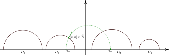
Figure 4. Sketch of a point $(z,v)$ in the fundamental domain $\widetilde{\Sigma}$ for the preimage of the Poincaré section $\Sigma$ together with its Hopf coordinates $(\gamma_{-},\gamma_{+})$ in the coordinate space $\bigcup_{i\neq j}I_{i}\times I_{j}$.

To leverage the simplicity of the geodesic flow in Hopf coordinates we choose an adapted distance function $\mathrm{d}_{G}$ in the following fashion: Denoting by $\mathrm{d}_{G/P}$ some $K$-invariant metric on the boundary of hyperbolic space let

$$\mathrm{d}_{G}(g,g^{\prime})^{2}\mathrel{\mathop{:}\!\!=}\mathrm{d}_{G/P}(g_{+},g^{\prime}_{+})^{2}+\mathrm{d}_{G/P}(g_{-},g^{\prime}_{-})^{2}+|t-t^{\prime}|^{2}$$

in the respective Hopf coordinates of $g$ and $g^{\prime}$. In terms of dynamics the resulting Gaussian amounts to a product of Gaussians in the contracting, expanding, and neutral (flow-) directions.

Remark 4.1.

Note that the resulting distance function is not analytic on the whole domain $\mathbb{R}\times(G/P)_{\Delta}$ if we make the obvious choice of angle coordinates on the unit circle $\mathrm{S}^{1}\cong G/P$ such that $\mathrm{d}_{G/P}^{2}$ becomes absolute value square on $[0,2\pi]$ with the endpoints identified. While this is certainly true we do not require this analyticity for an application of Corollary 2.4 but only the analyticity of the resulting potential as a function on the fundamental intervals $I_{i}$, c.f. the discussion surrounding (13). The final expression below will satisfy this analyticity making the theory of dynamical determinants developed above applicable here. From a theoretical standpoint the discussions involving the Poincaré section $\Sigma$ should be viewed more as an interpretation of what the potential given below means geometrically.

Having made the choices above we can now calculate $\mathrm{t}^{\Sigma}_{\lambda_{0},\sigma}\circ\mathcal{H}^{-1}|_{\mathcal{H}(\widetilde{\Sigma})}$ using dynamical determinants if we have suitable expressions for the following period integrals over closed geodesics $\gamma\subseteq S\mathbf{X}_{\Gamma}$:

$$\bigcup_{i\neq j}I_{i}\times I_{j}\ni(g_{+},g_{-})\mapsto\int_{\gamma}f_{\sigma,\mathcal{H}^{-1}(t(g_{+},g_{-}),g_{+},g_{-})}\leavevmode\nobreak\ .$$

First we may exploit $\Gamma$-invariance to re-write the integral as a sum over intersections with the fundamental domain. The argument here is quite similar to the previous Section 4.1. If the geodesic $\gamma$ is again represented by an isometry $g_{w}$, $w=(i_{1},\ldots,i_{n})\in\mathcal{W}_{n}$ then these intersections are determined by fixed points $(\gamma^{i}_{+},\gamma^{i}_{-})$ of cyclic permutations

$$g_{i_{n}}g_{i_{n-1}}\cdots g_{i_{1}},\leavevmode\nobreak\ g_{i_{1}}g_{i_{n}}\cdots g_{i_{2}},\leavevmode\nobreak\ g_{i_{2}}g_{i_{1}}g_{i_{n}}\cdots g_{i_{3}},\leavevmode\nobreak\ \text{etc.}\leavevmode\nobreak\ ,$$

and the period integrals become

$$\begin{split}&\quad\leavevmode\nobreak\ \int_{\gamma}f_{\sigma,\mathcal{H}^{-1}(t(g_{+},g_{-}),g_{+},g_{-})}\\ &=\mathcal{M}_{\sigma}^{-1}\sum_{i=1}^{n}\mathrm{e}^{-\frac{\mathrm{d}_{G/P}(g_{+},\gamma^{i}_{+})^{2}+\mathrm{d}_{G/P}(g_{-},\gamma^{i}_{-})^{2}}{\sigma^{2}}}\int_{-\infty}^{\infty}\mathrm{e}^{-\frac{|t(g_{+},g_{-})-t|^{2}}{\sigma^{2}}}\mathrm{d}t\leavevmode\nobreak\ .\end{split}$$

Here the second integral comes from taking the $t$-entry of Hopf coordinates for the lift $\widetilde{\gamma}^{i}$ of $\gamma$ with endpoints at infinity $(\gamma^{i}_{+},\gamma^{i}_{-})$ and integrating its distance from $t(g_{+},g_{-})$ over the whole geodesic $\widetilde{\gamma}^{i}$ of $\gamma$. If we combine this with an evaluation of the constant $\mathcal{M}_{\sigma}$, which reduces to iterated Gaussian integrals, our period integrals becomes the rather handy expression

$$\int_{\gamma}f_{\sigma,\mathcal{H}^{-1}(t(g_{+},g_{-}),g_{+},g_{-})}=\frac{1}{\pi\sigma^{2}}\sum_{i=1}^{n}\mathrm{e}^{-\frac{\mathrm{d}_{G/P}(g_{+},\gamma^{i}_{+})^{2}+\mathrm{d}_{G/P}(g_{+},\gamma^{i}_{-})^{2}}{\sigma^{2}}}\leavevmode\nobreak\ .$$ (22)

Again the approximation $\mathrm{t}^{\Sigma}_{\lambda_{0},\sigma}$ restricted to $\Sigma$ can be calculated via the residues of a weighted zeta function, concretely $Z_{f_{\sigma,\mathcal{H}^{-1}(t(g_{+},g_{-}),g_{+},g_{-})}}$. The latter is straightforward to implement using Snippet 1 but substituting the routine $\verb|calcInt|$ with an implementation of (22). Furthermore if we take Equation (22) as a definition it does indeed yield an analytic potential which makes Corollary 2.4 immediately applicable.

Remark 4.2.

Note that it is conceptually straight forward to replace the specific hypersurface $\Sigma$ with another choice $\Sigma^{\prime}$. One has to make sure that $\Sigma^{\prime}$ admits a family of test functions for which period integrals can be calculated efficiently. In most applications this should come down to finding an appropriate parametrization for $\Sigma^{\prime}$, adapting the test functions to this parametrization, and finally calculating the period integrals in this parametrization (using suitable approximations).

5. Symmetry Reduction of Weighted Zeta Functions

If we use the theoretical and practical tools developed up to this point it turns out that we require a large amount of closed geodesics and corresponding period integrals to compute the dynamical determinant with sufficient accuracy. In this section we will therefore develop a method that allows us to exploit inherent symmetries of different classes of Schottky surfaces to significantly reduce the required computational resources. Our approach to symmetry reduction essentially is an adaptation and generalization of similar work done by Borthwick and Weich [BW16] in the context of iterated function schemes. Even though these systems only incorporate an expanding direction it is quite straight forward to include the contracting direction present in the determinants constructed in Section 2.

Remark 5.1.

It should be rather straight forward to formulate and prove a version of the upcoming symmetry reduced dynamical determinant in the full setting of [Rug92]. We refrain from explicitly treating this greater generality here to keep the discussion aligned with the previous sections, in particular Section 2. A practically important generalization will instead be included in the first author’s PhD thesis, see also Section 6.

This section is organized as follows: In Section 5.1 we give some basic definitions and present the main theorem stating how our dynamical determinant $d_{f}$ decomposes as a product of symmetry reduced dynamical determinants with the product indexed by irreducible, unitary representations of some suitable symmetry group. While this theorem describes the theoretical situation completely it is not directly accessible to practical implementation. Section 5.2 remedies this by providing a detailed description how the symmetry reduction can be implemented. The final Section 5.3 contains a short comparison of the computational effort needed to calculate dynamical determinants with and without symmetry reduction.

5.1. Main Theorem

We begin by stating the fundamental definition of what the symmetry group of a particular representation of some Schottky surface should be [BW16, Theorem 3.1]:

Definition 5.2.

Let $\Gamma\subseteq\mathrm{SL}(2,\mathbb{R})$ be a rank-$r$ Schottky group with generators $g_{1},\ldots,g_{r}$ and fundamental discs $D_{1},\ldots,D_{2r}$. Let $\mathbf{G}$ be a finite group acting on $\bigcup_{i}D_{i}$ by holomorphic functions extending continuously to the boundary and define a $\mathbf{G}$-action on $\{1,\ldots,2r\}$ by the relation $\mathbf{g}(D_{i})=D_{\mathbf{g}\cdot i}$.

Then $\mathbf{G}$ is called a symmetry group of the generating set $\langle g_{1},...,g_{r}\rangle=\Gamma$ if for any $\mathbf{g}\in\mathbf{G}$ and $i\neq j\in\{1,\ldots,2r\}$ there exists an index $k\in\{1,\ldots,2r\}$ such that $k\neq\mathbf{g}\cdot i$ and

$$\mathbf{g}\cdot(g_{j}z)=g_{k}(\mathbf{g}\cdot z),\qquad\forall z\in D_{i}\leavevmode\nobreak\ ,$$

Because $\mathbf{g}\in\mathbf{G}$ acts on each disc as a biholomorphic map the image $\mathbf{g}(D_{i})$ must again be some disc making $\mathbf{g}\cdot i$ well-defined. The index $k$ in the relation $\mathbf{g}\cdot(g_{j}z)=g_{k}(\mathbf{g}\cdot z)$ is unique and we observe that $k=\mathbf{g}\cdot j$. Furthermore the group action of $\mathbf{G}$ on the elements of $\mathbb{Z}/2r\mathbb{Z}$ takes distinct pairs of indices $i\neq j$ to distinct pairs: $\mathbf{g}\cdot i\neq\mathbf{g}\cdot j$. The action of an element $\mathbf{g}\in\mathbf{G}$ can then be written concisely as

$$\mathbf{g}\cdot(g_{j}z)=g_{\mathbf{g}\cdot j}(\mathbf{g}\cdot z),\qquad\forall z\in D_{i},\,j\neq i\leavevmode\nobreak\ .$$

We extend this action to $(\mathbb{Z}/2r\mathbb{Z})^{n}$ (or $\mathcal{W}_{n}$) by acting on each element separately.

The desired composition of our dynamical (Fredholm) determinants now follows from the rather simple representation theory of finite groups by observing that $\mathbf{G}$ acts on the function spaces introduced in Section 2.1 via the left-regular representation:

$$\left\langle\mathbf{g}\cdot u(z_{1},z_{2}),v(z_{1})\right\rangle\mathrel{\mathop{:}\!\!=}\left\langle u(\mathbf{g}^{-1}\cdot z_{1},\mathbf{g}^{-1}\cdot z_{2}),v(z_{1})\right\rangle,\qquad u\in\bigoplus_{i\neq j}\mathcal{H}^{-2}(D_{i})\otimes\mathcal{H}^{2}(D_{j})\leavevmode\nobreak\ .$$

This representation will generally not be unitary because we defined the $\mathrm{L}^{2}$-scalar product via Lebesgue measure. The standard trick of averaging the pushforward of Lebesgue measure over the finite group $\mathbf{G}$ guarantees unitary, though. This yields a modified Bergman space which contains the same functions but whose scalar product differs from the standard one used so far by some smooth density factor.

Well known representation theory of finite groups [FH04, Part I] now provides a direct sum decomposition of this modified Bergman space indexed by characters $\chi$ of (equivalence classes $\widehat{\mathbf{G}}$ of) irreducible, unitary representations of $\mathbf{G}$ with the projectors on the individual summands given by

$$\mathrm{P}_{\chi}\mathrel{\mathop{:}\!\!=}\frac{d_{\chi}}{|\mathbf{G}|}\sum_{\mathbf{g}\in\mathbf{G}}\overline{\chi(\mathbf{g})}\mathbf{g}\leavevmode\nobreak\ .$$

In this equation $d_{\chi}$ refers to the dimension of the representation with character $\chi$ and $|\mathbf{G}|$ denotes the cardinality of $\mathbf{G}$. As the projections do not involve the scalar product we immediately derive a corresponding non-orthogonal direct sum decomposition of our original Hilbert spaces:

$$\bigoplus_{i\neq j}\mathcal{H}^{-2}(D_{i})\otimes\mathcal{H}^{2}(D_{j})=\bigoplus_{\chi\in\widehat{\mathbf{G}}}\mathcal{H}_{\chi},\qquad\mathcal{H}_{\chi}\mathrel{\mathop{:}\!\!=}\mathrm{P}_{\chi}\bigg{(}\bigoplus_{i\neq j}\mathcal{H}^{-2}(D_{i})\otimes\mathcal{H}^{2}(D_{j})\bigg{)}\leavevmode\nobreak\ .$$

The transfer operator $\mathrm{L}_{V}$ defined in Section 2.1 now commutes with the action of $\mathbf{G}$ if the potential $V$ is $\mathbf{G}$-invariant, i.e. $V(\mathbf{g}^{-1}\cdot z_{1},\mathbf{g}^{-1}\cdot z_{2})=V(z_{1},z_{2})$:

$$\begin{split}&\qquad\left\langle\mathrm{L}_{V}(\mathbf{g}\cdot u)(z_{1},z_{2}),v(z_{1})\right\rangle\bigg{|}_{\begin{subarray}{c}v\in\mathcal{H}^{2}(D_{i})\\ z_{2}\in D_{j}\end{subarray}}\\ &=\int_{\partial D_{i}}u(\mathbf{g}^{-1}\cdot g_{i}(z_{1}),\mathbf{g}^{-1}\cdot g_{i}(z_{2}))V(z_{1},z_{2})v(z_{1})\frac{\mathrm{d}z_{1}}{2\pi\mathrm{i}}\\ &=\int_{\partial D_{i}}u(g_{\mathbf{g}^{-1}\cdot i}(\mathbf{g}^{-1}\cdot z_{1}),g_{\mathbf{g}^{-1}\cdot i}(\mathbf{g}^{-1}\cdot z_{2}))V(\mathbf{g}^{-1}\cdot z_{1},\mathbf{g}^{-1}\cdot z_{2})v(z_{1})\frac{\mathrm{d}z_{1}}{2\pi\mathrm{i}}\\ &=\left\langle\mathbf{g}\cdot\big{(}\mathrm{L}_{V}u\big{)}(z_{1},z_{2}),v(z_{1})\right\rangle\bigg{|}_{\begin{subarray}{c}v\in\mathcal{H}^{2}(D_{i})\\ z_{2}\in D_{j}\end{subarray}}\leavevmode\nobreak\ .\end{split}$$

From this it is obvious that $\mathrm{L}_{V}$ commutes with the projections $\mathrm{P}_{\chi}$ which makes the subspaces $\mathcal{H}_{\chi}$ invariant under $\mathrm{L}_{V}$. This simple observation is already the key to the main factorization theorem of this section. Before we can state said theorem we need one additional definition: Given an element $\mathbf{g}\in\mathbf{G}$ we define a symmetry adapted version of $\mathcal{W}_{n}$ as follows

$$\mathcal{W}^{\mathbf{g}}_{n}\mathrel{\mathop{:}\!\!=}\big{\{}(i_{1},\ldots,i_{n})\in(\mathbb{Z}/2r\mathbb{Z})^{n}\,\big{|}\,i_{j}\neq i_{j+1}+r\,\forall\,j\in\{1,\ldots,n-1\},\,\mathbf{g}\cdot i_{n}\neq i_{1}+r\big{\}}\leavevmode\nobreak\ .$$

In unison with [BW16] we refer to elements of $\mathcal{W}^{\mathbf{g}}_{n}$ as $\mathbf{g}$-closed words of length $n$.

For the main theorem first note that $g_{w}\circ\mathbf{g}$ has a unique pair of repelling and attracting fixed points $x^{w,\mathbf{g}}_{-}\in D_{i_{n}+r}$ and $x^{w,\mathbf{g}}_{+}\in D_{\mathbf{g}^{-1}\cdot i_{1}}$ because $\mathbf{g}$ is biholomorphic and the same argument as in [BW16, Lemma 2.6] can be applied with domains $D_{i_{n}+r}$ and $D_{\mathbf{g}^{-1}\cdot i_{1}}$. It can be stated as follows:

Theorem 5.3 ([BW16], Prop. 3.3 and Thm. 4.1).

Let $\Gamma$ be a Schottky group with symmetry group $\mathbf{G}$ and $V$ a $\mathbf{G}$-invariant potential which is analytic in a neighborhood of the fundamental circles. Then the Fredholm determinant of the transfer operator $\mathrm{L}_{V}$ factorizes as

$$\det\left(\mathrm{id}-z\mathrm{L}_{V}\right)=\prod_{\chi\in\widehat{\mathbf{G}}}d_{V,\chi}(z)\leavevmode\nobreak\ ,$$

where for sufficiently small $|z|$ the symmetry reduced determinants $d_{V,\chi}$ are explicitly given by the following expressions:

$$d_{V,\chi}(z)=\exp\left(-\sum_{n=1}^{\infty}\frac{z^{n}}{n}\frac{d_{\chi}}{|\mathbf{G}|}\sum_{\mathbf{g}\in\mathbf{G}}\chi(\mathbf{g})\sum_{w\in\mathcal{W}^{\mathbf{g}}_{n}}\frac{V_{w}(\mathbf{g}\cdot x^{w,\mathbf{g}}_{-},\mathbf{g}\cdot x^{w,\mathbf{g}}_{+})}{((g_{w}\circ\mathbf{g})^{\prime}(x^{w,\mathbf{g}}_{-})-1)(1-(g_{w}\circ\mathbf{g})^{\prime}(x^{w,\mathbf{g}}_{+}))}\right)\leavevmode\nobreak\ .$$

Proof.

By the previously discussed decomposition of the domain of $\mathrm{L}_{V}$ into the direct sum $\bigoplus_{\chi\in\widehat{\mathbf{G}}}\mathcal{H}_{\chi}$ it is clear that

$$\det\left(\mathrm{id}-z\mathrm{L}_{V}\right)=\prod_{\chi\in\widehat{\mathbf{G}}}\det\left(\mathrm{id}-z\mathrm{L}_{V}\big{|}_{\mathcal{H}_{\chi}}\right)\leavevmode\nobreak\ .$$

We are therefore tasked with computing $d_{V,\chi}(z)\mathrel{\mathop{:}\!\!=}\det\big{(}\mathrm{id}-z\mathrm{L}_{V}\big{|}_{\mathcal{H}_{\chi}}\big{)}$. This Fredholm determinant can be expressed in terms of traces of $n$-fold iterates just as in (9). The key is therefore evaluating

$$\mathrm{Tr}\bigg{(}\mathrm{L}_{V}^{n}\big{|}_{\mathcal{H}_{\chi}}\bigg{)}=\mathrm{Tr}\big{(}\mathrm{P}_{\chi}\mathrm{L}_{V}^{n}\big{)}\leavevmode\nobreak\ ,$$

where the equality immediately follows from the fact that $\mathrm{L}_{V}$ commutes with the projections $\mathrm{P}_{\chi}$ and the trace-class property is inherited from $\mathrm{L}^{n}_{V}$.

Now the (diagonal) components of $n$-fold iterates of $\mathrm{L}_{V}$ were already calculated in (10). A very similar calculation yields, after replacing the sum over $\mathbf{g}$ by with a sum over $\mathbf{g}^{-1}$, the following expression:

$$\mathrm{Tr}\bigg{(}\mathrm{L}_{V}^{n}\big{|}_{\mathcal{H}_{\chi}}\bigg{)}=\frac{d_{\chi}}{|\mathbf{G}|}\sum_{\mathbf{g}\in\mathbf{G}}\chi(\mathbf{g})\sum_{w\in\mathcal{W}^{\mathbf{g}}_{n}}\mathrm{Tr}\big{(}\mathrm{L}_{V,\mathbf{g}}^{w}\big{)}\leavevmode\nobreak\ ,$$

where the modified diagonal components $\mathrm{L}_{V,\mathbf{g}}^{w}$, $w\in\mathcal{W}^{\mathbf{g}}_{n}$, are operators of the form

$$\left\langle\mathrm{L}_{V,\mathbf{g}}^{w}u(z_{1},z_{2}),v(z_{1})\right\rangle\bigg{|}_{\begin{subarray}{c}v\in\mathcal{H}^{2}(D_{i_{n}+r})\\ z_{2}\in D_{\mathbf{g}^{-1}i_{1}}\end{subarray}}=\int_{\partial D_{i_{n}+r}}V_{g}(\mathbf{g}\cdot z_{1},\mathbf{g}\cdot z_{2})u(g_{w}(\mathbf{g}\cdot z_{1}),g_{w}(\mathbf{g}\cdot z_{2}))v(z_{1})\frac{\mathrm{d}z_{1}}{2\pi\mathrm{i}}\leavevmode\nobreak\ .$$

Here the traces of these operators can be calculated in complete analogy to Theorem 2.2 but now the pair of fixed points $x^{w,\mathbf{g}}_{-}\in D_{i_{n}+r}$ and $x^{w,\mathbf{g}}_{+}\in D_{\mathbf{g}^{-1}\cdot i_{1}}$ of the holomorphic map $g_{w}\circ\mathbf{g}$ appears. We finally obtain

$$\mathrm{Tr}\left(\mathrm{L}^{w}_{V,\mathbf{g}}\right)=\frac{V_{w}(\mathbf{g}\cdot x^{w,\mathbf{g}}_{-},\mathbf{g}\cdot x^{w,\mathbf{g}}_{+})}{((g_{w}\circ\mathbf{g})^{\prime}(x^{w,\mathbf{g}}_{-})-1)(1-(g_{w}\circ\mathbf{g})^{\prime}(x^{w,\mathbf{g}}_{+}))}\leavevmode\nobreak\ ,$$

which finishes the proof. ∎

5.2. Implementation Details

One of the key observations in [BW16] is a clever grouping of terms in $d_{V,\chi}$. On the one hand it provides convergence beyond small $|z|$ and on the other hand it speeds up the practical computation of symmetry reduced zeta functions tremendously. An adaptation of this work allows us to achieve both these benefits for our weighted zeta functions as well. The following presentation closely follows [BW16, Sections 4–5].

To meet our objective we first introduce some additional notation: Observing that elements $w\in\mathcal{W}_{n}^{\mathbf{g}}$ always occur together with their closing group element $\mathbf{g}$ in Theorem 5.3 it makes sense to define

$$\mathcal{W}^{\mathbf{G}}\mathrel{\mathop{:}\!\!=}\left\{(w,\mathbf{g})\in\bigg{(}\bigcup_{n=1}^{\infty}\mathcal{W}_{n}\bigg{)}\times\mathbf{G}\,\bigg{|}\,\mathbf{g}\cdot w_{n_{w}}\neq w_{1}+r\right\}\leavevmode\nobreak\ ,$$

where $n_{w}$ denotes the length of $w$, i.e. $w\in\mathcal{W}_{n_{w}}$, and we index words as $w=(w_{1},\ldots,w_{n_{w}})$. We will henceforth denote elements of $\mathcal{W}^{\mathbf{G}}$ by boldface letters and indicate their first and second components by the corresponding non-boldface letter and a suitable subscript: $\mathbf{w}=(w,\mathbf{g}_{\mathbf{w}})\in\mathcal{W}^{\mathbf{G}}$. This definition immediately allows us to shorten the notation for fixed points introduced in the previous section by setting $x^{\mathbf{w}}_{\pm}\mathrel{\mathop{:}\!\!=}x^{w,\mathbf{g}_{\mathbf{w}}}_{\pm}$.

The actual regrouping of terms now happens due to a derived action of $\mathbf{G}\times\mathbb{Z}$ on $\mathcal{W}^{\mathbf{G}}$ which we will describe next. First of all an element $\mathbf{h}\in\mathbf{G}$ acts on $\mathcal{W}^{\mathbf{G}}$ via

$$\mathbf{h}\cdot\mathbf{w}=\mathbf{h}\cdot(w,\mathbf{g}_{\mathbf{w}})\mathrel{\mathop{:}\!\!=}(\mathbf{h}\cdot w,\mathbf{h}\mathbf{g}_{\mathbf{w}}\mathbf{h}^{-1})\leavevmode\nobreak\ .$$

This action is complemented by the $\mathbb{Z}$-action generated by the two (inverse) shifts acting in the first component as

$$\begin{split}\sigma_{R}\mathbf{w}&\mathrel{\mathop{:}\!\!=}\big{(}(\mathbf{g}_{\mathbf{w}}w_{n},w_{1},\ldots,w_{n-1}),\mathbf{g}_{\mathbf{w}}\big{)}\leavevmode\nobreak\ ,\\ \sigma_{L}\mathbf{w}&\mathrel{\mathop{:}\!\!=}\big{(}(w_{2},\ldots,w_{n},\mathbf{g}_{\mathbf{w}}^{-1}w_{1}),\mathbf{g}_{\mathbf{w}}\big{)}\leavevmode\nobreak\ .\end{split}$$

This $\mathbb{Z}$-action commutes with the action of $\mathbf{G}$. We can therefore consider the space $\big{[}\mathcal{W}^{\mathbf{G}}\big{]}\mathrel{\mathop{:}\!\!=}(\mathbf{G}\times\mathbb{Z})\setminus\mathcal{W}^{\mathbf{G}}$ of orbits under the product of these actions and we denote the equivalence class containing $\mathbf{w}\in\mathcal{W}^{\mathbf{G}}$ by $[\mathbf{w}]$.

Before we can re-organize the sums appearing in Theorem 5.3 it remains to identify an appropriate notion of composite elements. To this end we define the $k$-fold iteration of $\mathbf{w}\in\mathcal{W}^{\mathbf{G}}$ by the formula

$$\mathbf{w}^{k}\mathrel{\mathop{:}\!\!=}\big{(}(\mathbf{g}_{\mathbf{w}}^{k-1}w_{1},\ldots,\mathbf{g}_{\mathbf{w}}^{k-1}w_{n},\mathbf{g}_{\mathbf{w}}^{k-2}w_{1},\ldots,\mathbf{g}_{\mathbf{w}}w_{1},\ldots,\mathbf{g}_{\mathbf{w}}w_{n},w_{1},\ldots w_{n}),\mathbf{g}_{\mathbf{w}}^{k}\big{)}\leavevmode\nobreak\ ,$$

and we call an element of $\mathcal{W}^{\mathbf{G}}$ prime if it cannot be represented as such an iteration for $k>1$. Otherwise we call the element composite.

Next we recall some features of the various notions just introduced. Complete proofs can be found in [BW16, Lemma 4.3, Prop. 4.4]. We continue to denote by $V(z_{1},z_{2})$ some $\mathbf{G}$-invariant potential.

1. An orbit of the $\mathbf{G}\times\mathbb{Z}$-action consists either entirely of prime or entirely of composite elements making $\left[\mathcal{W}^{\mathbf{G}}_{\mathrm{p}}\right]\mathrel{\mathop{:}\!\!=}\{[\mathbf{w}]\,|\,w\leavevmode\nobreak\ \text{prime}\}$ well-defined;

2. Given $\mathbf{v}\in[\mathbf{w}^{k}]$ one has the equalities $V_{v}(\mathbf{g}_{\mathbf{v}}x^{\mathbf{v}}_{-},\mathbf{g}_{\mathbf{v}}x^{\mathbf{v}}_{+})=V_{w}(\mathbf{g}_{\mathbf{w}}x^{\mathbf{w}}_{-},\mathbf{g}_{\mathbf{w}}x^{\mathbf{w}}_{+})^{k}$ and $(g_{v}\circ\mathbf{g}_{\mathbf{v}})^{\prime}(x^{\mathbf{v}}_{\pm})=(g_{w}\circ\mathbf{g}_{\mathbf{w}})^{\prime}(x^{\mathbf{w}}_{\pm})^{k}$;

3. If $\mathbf{G}$ acts freely on $\mathcal{W}^{\mathbf{G}}$ then the number of elements in the equivalence class $[\mathbf{w}]\in\big{[}\mathcal{W}^{\mathbf{G}}_{\mathrm{p}}\big{]}$ can be calculated as $\#[\mathbf{w}]=|\mathbf{G}|\cdot n_{\mathbf{w}}$;

4. If $m_{\mathbf{w}}\mathrel{\mathop{:}\!\!=}\mathrm{ord}(\mathbf{g})$ denotes the order of $\mathbf{g}\in\mathbf{G}$ then the equalities $(g_{w}\circ\mathbf{g}_{\mathbf{w}})^{\prime}(x^{\mathbf{w}}_{\pm})=g_{w^{m_{\mathbf{w}}}}^{\prime}(x^{w^{m_{\mathbf{w}}}}_{\pm})^{1/m_{\mathbf{w}}}$ and $V_{w}(\mathbf{g}_{\mathbf{w}}\cdot x^{\mathbf{w}}_{\pm})=V_{w^{m_{\mathbf{w}}}}(x^{w^{m_{\mathbf{w}}}}_{\pm})^{1/m_{\mathbf{w}}}$ hold for any $[\mathbf{w}]\in\big{[}\mathcal{W}^{\mathbf{G}}_{\mathrm{p}}\big{]}$ and denoting by $x^{v}_{\pm}$ the fixed points of $g_{v}$.

With this we can now reformulate Theorem 5.3 in a form which is very reminiscent of our definition of the dynamical determinant $d_{f}$ in (5). From the preceding discussion combined with Theorem 5.3 and under the assumptions of $\mathbf{G}$-invariant potential and free $\mathbf{G}$-action on $\mathcal{W}^{\mathbf{G}}$ we immediately deduce the following for sufficiently small $|z|$

$$\begin{split}d_{V,\chi}(z)&=\exp\left(-d_{\chi}\sum_{[\mathbf{w}]\in\big{[}\mathcal{W}^{\mathbf{G}}\big{]}}\frac{\#[\mathbf{w}]\cdot z^{n_{\mathbf{w}}}}{n_{\mathbf{w}}\cdot|\mathbf{G}|}\frac{\chi(\mathbf{g}_{\mathbf{w}})V_{w}(\mathbf{g}_{\mathbf{w}}\cdot x^{\mathbf{w}}_{-},\mathbf{g}_{\mathbf{w}}\cdot x^{\mathbf{w}}_{+})}{((g_{w}\circ\mathbf{g}_{\mathbf{w}})^{\prime}(x^{\mathbf{w}}_{-})-1)(1-(g_{w}\circ\mathbf{g}_{\mathbf{w}})^{\prime}(x^{\mathbf{w}}_{+}))}\right)\\ &=\exp\left(-d_{\chi}\sum_{k=1}^{\infty}\sum_{[\mathbf{w}]\in\big{[}\mathcal{W}^{\mathbf{G}}_{\mathrm{p}}\big{]}}\frac{\#[\mathbf{w}^{k}]z^{kn_{\mathbf{w}}}}{kn_{\mathbf{w}}|\mathbf{G}|}\frac{\chi(\mathbf{g}_{\mathbf{w}}^{k})\cdot V_{w}(\mathbf{g}_{\mathbf{w}}\cdot x^{\mathbf{w}}_{-},\mathbf{g}_{\mathbf{w}}\cdot x^{\mathbf{w}}_{+})^{k}}{((g_{w}\circ\mathbf{g}_{\mathbf{w}})^{\prime}(x^{\mathbf{w}}_{-})^{k}-1)(1-(g_{w}\circ\mathbf{g}_{\mathbf{w}})^{\prime}(x^{\mathbf{w}}_{+})^{k})}\right)\\ &=\exp\left(-d_{\chi}\sum_{k=1}^{\infty}\sum_{[\mathbf{w}]\in\big{[}\mathcal{W}^{\mathbf{G}}_{\mathrm{p}}\big{]}}\frac{z^{kn_{\mathbf{w}}}}{k}\frac{\chi(\mathbf{g}_{\mathbf{w}}^{k})\cdot V_{w^{m_{\mathbf{w}}}}(x^{w^{m_{\mathbf{w}}}}_{-},x^{w^{m_{\mathbf{w}}}}_{+})^{k/m_{\mathbf{w}}}}{\big{(}\mathrm{e}^{kT_{\gamma(g_{w^{m_{\mathbf{w}}}})}/m_{\mathbf{w}}}-1\big{)}\big{(}1-\mathrm{e}^{-kT_{\gamma(g_{w^{m_{\mathbf{w}}}})}/m_{\mathbf{w}}}\big{)}}\right)\leavevmode\nobreak\ .\end{split}$$ (23)

From here we can proceed by applying the cycle expansion philosophy introduced in Section 3. This results in the following Proposition which generalizes Corollaries 2.5 as well as 3.1 and serves as our primary tool for practical implementation. We require a final definition before presenting the actual statement: Given a weight function $f\in\mathrm{C}^{\omega}(S\mathbf{X}_{\Gamma})$ we say that it has $\mathbf{G}$-invariant period integrals if its integrals over closed geodesics satisfy

$$\int_{\gamma(g_{w})}f=\int_{\gamma(g_{\mathbf{g}\cdot w})}f\leavevmode\nobreak\ ,\qquad\forall\mathbf{g}\in\mathbf{G},\,\forall w\in\mathcal{W}_{n}\leavevmode\nobreak\ .$$

The main example for this is given by the case where $\mathbf{G}$ even acts on the whole unit sphere bundle $S\mathbf{H}$. It then acts on $\Gamma$-invariant elements of $\mathrm{C}^{\infty}(S\mathbb{H})$ by translation and if $f$ is invariant under this $\mathbf{G}$-action then it also has $\mathbf{G}$-invariant period integrals because $\gamma(g_{\mathbf{g}\cdot w})=\mathbf{g}\cdot\gamma(g_{w})$ in this setting.

The central proposition now reads as follows:

Proposition 5.4.

Let $\Gamma$ be a Schottky group with symmetry group $\mathbf{G}$ acting freely on $\mathcal{W}^{\mathbf{G}}$ and $f\in\mathrm{C}^{\omega}(S\mathbf{X}_{\Gamma})$ an analytic weight with $\mathbf{G}$-invariant period integrals. Then the following hold:

1. The dynamical determinant decomposes as a product

   $$d_{f}(\lambda,z,\beta)=\prod_{\chi\in\widehat{\mathbf{G}}}d_{f,\chi}(\lambda,z,\beta)$$

   of symmetry reduced dynamical determinants $d_{f,\chi}$.

2. The $d_{f,\chi}$ are given by an everywhere convergent power series expansion

   $$d_{f,\chi}(\lambda,z,\beta)=1+\sum_{n=1}^{\infty}d_{n}^{\chi}(\lambda,\beta)z^{n}\leavevmode\nobreak\ ,$$

   with coefficients in this expansion being holomorphic functions in $(\lambda,\beta)$ and explicitly given by the recursion

   $$\begin{split}d_{n}^{\chi}(\lambda,\beta)&=\sum_{m=1}^{n}\frac{m}{n}d_{n-m}^{\chi}(\lambda,\beta)a_{m}^{\chi}(\lambda,\beta)\leavevmode\nobreak\ ,\qquad d_{0}^{\chi}(\lambda,\beta)\equiv 1\leavevmode\nobreak\ ,\\ a_{m}^{\chi}(\lambda,\beta)&=-d_{\chi}\sum_{\begin{subarray}{c}([\mathbf{w}],k)\in\big{[}\mathcal{W}^{\mathbf{G}}_{\mathrm{p}}\big{]}\times\mathbb{N}_{>0}\\ n_{\mathbf{w}}\cdot k=m\end{subarray}}\frac{\chi(\mathbf{g}_{\mathbf{w}}^{k})}{k}\frac{\exp\big{(}-\frac{k(\lambda-1)}{m_{\mathbf{w}}}T_{\gamma(g_{w^{m_{\mathbf{w}}}})}-\frac{k\beta}{m_{\mathbf{w}}}\int_{\gamma(g_{w^{m_{\mathbf{w}}}})}f\big{)}}{\big{(}\mathrm{e}^{kT_{\gamma(g_{w^{m_{\mathbf{w}}}})}/m_{\mathbf{w}}}-1\big{)}^{2}}\leavevmode\nobreak\ .\end{split}$$

   The coefficients $d_{n}^{\chi}(\lambda,\beta)$ satisfies super-exponential bounds of the same kind as in Corollary 3.1.

3. The weighted zeta function $Z_{f}$ decomposes as a sum of meromorphic functions given by logarithmic derivatives of the $d_{f,\chi}$:

   $$Z_{f}(\lambda)=\sum_{\chi\in\widehat{\mathbf{G}}}\frac{\partial_{\beta}d_{f,\chi}(\lambda,1,0)}{d_{f,\chi}(\lambda,1,0)}\leavevmode\nobreak\ .$$

Proof.

The idea of proof is very much aligned with the material presented in Sections 2 and 3: To derive (1) we would like to plug the concrete potential of Corollary 2.4 into the product decomposition of Theorem 5.3.

A slight difficulty with this strategy is the fact that the potential $V_{\lambda,\beta}$ of Corollary 2.4 is not $\mathbf{G}$-invariant due to the presence of the derivative term. This can be remedied by substituting it with a $\mathbf{G}$-averaged version possessing built-in $\mathbf{G}$-invariant, c.f. [BW16, Lemma 5.6]:

$$V_{\lambda,\beta}^{\mathbf{G}}\mathrel{\mathop{:}\!\!=}\prod_{\mathbf{g}\in\mathbf{G}}V_{\lambda,\beta}(\mathbf{g}\cdot z_{1},\mathbf{g}\cdot z_{2})^{1/|\mathbf{G}|}\leavevmode\nobreak\ .$$

By (7) we only need to verify $(V_{\lambda,\beta})_{w}=(V_{\lambda,\beta}^{\mathbf{G}})_{w}$ for any closed word $w\in\mathcal{W}_{n}$ to prove that the transfer operators associated with these potentials give rise to the same Fredholm determinant. Using the $\mathbf{G}$-invariance of the period integrals of $f$ and the proof of [BW16, Lemma 5.6] (which is essentially an application of the ordinary chain rule) we can now calculate

$$\begin{split}\big{(}V_{\lambda,\beta}^{\mathbf{G}}\big{)}_{w}&=\exp\left(-\frac{\beta}{|\mathbf{G}|}\sum_{\mathbf{g}\in\mathbf{G}}\int_{\gamma(g_{\mathbf{g}\cdot w})}f\right)\cdot\mathrm{e}^{-\lambda T_{\gamma(g_{w})}}\\ &=\exp\left(-\lambda T_{\gamma(g_{w})}-\beta\int_{\gamma(g_{w})}f\right)=\big{(}V_{\lambda,\beta}\big{)}_{w}\leavevmode\nobreak\ .\end{split}$$

This proves (1) if we define $d_{f,\chi}(\lambda,z,\beta)\mathrel{\mathop{:}\!\!=}d_{V_{\lambda,\beta}^{\mathbf{G}},\chi}(z)$.

To obtain the expression for $d_{f,\chi}(\lambda,z,\beta)$ claimed in (2), we start with the following formula derived for a general potential in (23) above and valid for sufficiently small $|z|$

$$\begin{split}d_{f,\chi}(\lambda,z,\beta)&=\exp\left(-d_{\chi}\sum_{k=1}^{\infty}\sum_{[\mathbf{w}]\in\big{[}\mathcal{W}^{\mathbf{G}}_{\mathrm{p}}\big{]}}\frac{z^{kn_{\mathbf{w}}}}{k}\frac{\chi(\mathbf{g}_{\mathbf{w}}^{k})\cdot\exp\big{(}-\frac{k\lambda}{m_{\mathbf{w}}}T_{\gamma(g_{w^{m_{\mathbf{w}}}})}-\frac{k\beta}{m_{\mathbf{w}}}\int_{\gamma(g_{w^{m_{\mathbf{w}}}})}f\big{)}}{\big{(}\mathrm{e}^{kT_{\gamma(g_{w^{m_{\mathbf{w}}}})}/m_{\mathbf{w}}}-1\big{)}\big{(}1-\mathrm{e}^{-kT_{\gamma(g_{w^{m_{\mathbf{w}}}})}/m_{\mathbf{w}}}\big{)}}\right)\\ &=\exp\left(\sum_{n=1}^{\infty}a_{n}^{\chi}(\lambda,\beta)z^{n}\right)\leavevmode\nobreak\ ,\end{split}$$

with the definition

$$a_{n}^{\chi}(\lambda,\beta)\mathrel{\mathop{:}\!\!=}-d_{\chi}\sum_{\begin{subarray}{c}([\mathbf{w}],k)\in\big{[}\mathcal{W}^{\mathbf{G}}_{\mathrm{p}}\big{]}\times\mathbb{N}_{>0}\\ n_{\mathbf{w}}\cdot k=n\end{subarray}}\frac{\chi(\mathbf{g}_{\mathbf{w}}^{k})}{k}\frac{\exp\big{(}-\frac{k\lambda}{m_{\mathbf{w}}}T_{\gamma(g_{w^{m_{\mathbf{w}}}})}-\frac{k\beta}{m_{\mathbf{w}}}\int_{\gamma(g_{w^{m_{\mathbf{w}}}})}f\big{)}}{\big{(}\mathrm{e}^{kT_{\gamma(g_{w^{m_{\mathbf{w}}}})}/m_{\mathbf{w}}}-1\big{)}\big{(}1-\mathrm{e}^{-kT_{\gamma(g_{w^{m_{\mathbf{w}}}})}/m_{\mathbf{w}}}\big{)}}\leavevmode\nobreak\ .$$

The theory of Bell polynomials already used in the proof of Corollary 3.1 now yields the claimed recursive relation.

The super-exponential bounds can be derived in the same manner as in Corollary 3.1 by simply observing that the singular values of the restrictions satisfy $\mu_{i}(\mathrm{P}_{\chi}\mathrm{L}_{V})\leq\Arrowvert\mathrm{P}_{\chi}\Arrowvert\mu_{i}(\mathrm{L}_{V})$. We can therefore recycle our previous calculations and arrive at the same bounds with possibly different constants.

Lastly we derive (3) in the following straightforward manner: Exchanging the logarithm of the product over $\widehat{\mathbf{G}}$ with a sum over logarithms in Corollary 2.5 lets us calculate

$$\begin{split}Z_{f}(\lambda)&=\partial_{\beta}\log\left(\det\big{(}\mathrm{id}-z\mathrm{L}_{\lambda,\beta}^{f}\big{)}\right)\bigg{|}_{z=1,\beta=0}\\ &=\partial_{\beta}\log\left(\det\big{(}\mathrm{id}-z\mathrm{L}_{V_{\lambda,\beta}^{\mathbf{G}}}\big{)}\right)\bigg{|}_{z=1,\beta=0}\\ &=\sum_{\chi\in\widehat{\mathbf{G}}}\partial_{\beta}\log\left(d_{f,\chi}(\lambda,z,\beta)\right)\bigg{|}_{z=1,\beta=0}\leavevmode\nobreak\ ,\end{split}$$

finishing our proof. ∎

For practical purposes the following form for the coefficients occurring in the base of the recursion is more suitable:

$$\begin{split}a_{m}^{\chi}(\lambda,\beta)&=-\frac{d_{\chi}}{m}\sum_{\begin{subarray}{c}[\mathbf{w}]\in\big{[}\mathcal{W}^{\mathbf{G}}_{\mathrm{p}}\big{]}\\ n_{\mathbf{w}}||m\end{subarray}}n_{\mathbf{w}}\cdot\chi(\mathbf{g}_{\mathbf{w}}^{m/n_{\mathbf{w}}})\frac{\exp\big{(}-\frac{m(\lambda-1)}{n_{\mathbf{w}}m_{\mathbf{w}}}T_{\gamma(g_{w^{m_{\mathbf{w}}}})}-\frac{m\beta}{n_{\mathbf{w}}m_{\mathbf{w}}}\int_{\gamma(g_{w^{m_{\mathbf{w}}}})}f\big{)}}{\big{(}\mathrm{e}^{mT_{\gamma(g_{w^{m_{\mathbf{w}}}})}/(n_{\mathbf{w}}m_{\mathbf{w}})}-1\big{)}^{2}}\leavevmode\nobreak\ ,\end{split}$$

where $n||m$ for $n,m\in\mathbb{N}$ indicates that $n$ divides $m$. Rescaling both lengths and period integrals by $1/(n_{\mathbf{w}}m_{\mathbf{w}})$ like this yields a rather convenient way for vectorized evaluation of the coefficients $a_{m}^{\chi}$.

Remark 5.5.

The proposition does not reveal if and why any improvement in terms of convergence should be expected from the coefficients $d_{n}^{\chi}$ compared with their non-symmetry reduced counterparts $d_{n}$. The practical calculations below will reveal a significant improvement, though. For a theoretical discussion of this phenomenon we refer to [BW16, Appendix B].

Remark 5.6.

If we want to apply Proposition 5.4 we have to adjust the families of test functions presented in Section 4 to satisfy $\mathbf{G}$-invariance of their period integrals. But this is fairly straightforward: We simply replace the expressions derived in (20) and (22) by similar sums but over points $x_{j}+\mathrm{i}y_{j}$ or $(\gamma^{i}_{-},\gamma^{i}_{+})$, respectively, derived not only from the original word $w$ but from all words $\mathbf{g}\cdot w$ for $\mathbf{g}\in\mathbf{G}$. A subsequent normalization by $|\mathbf{G}|$ then yields a suitable prescription.

Input: width $\sigma>0$, center $gK\in G/K$, resonance $\lambda_{0}\in\mathbb{C}$, character $\chi\in\widehat{\mathbf{G}}$, cut-off $N\in\mathbb{N}$

/* calculate Bell recursion as in Snippet 1, but with $a[]$ replaced by modified initial terms $a^{\chi}[]$ */

/* calculate modified initial terms $a^{\chi}[k]$ in Bell recursion */

$a^{\chi}[k]\leftarrow 0$;

$\partial a^{\chi}[k]\leftarrow 0$;

for $[\mathbf{w}]\in\left[\mathcal{W}_{p}^{\mathbf{G}}\right]\leavevmode\nobreak\ \mathrm{where}\leavevmode\nobreak\ n_{\mathbf{w}}||k$ do

       $a^{\chi}[k]\leftarrow a^{\chi}[k]-n_{\mathbf{w}}\chi(\mathbf{g}_{\mathbf{w}}^{k/n_{\mathbf{w}}})\frac{\exp(-(\lambda_{0}-1)k\ell(g_{w})/(n_{\mathbf{w}}m_{\mathbf{w}}))}{(\mathrm{e}^{k\ell(g_{w})/(n_{\mathbf{w}}m_{\mathbf{w}})}-1)^{2}}$;

       $\partial_{\beta}a[k]\leftarrow\partial_{\beta}a[k]+n_{\mathbf{w}}\chi(\mathbf{g}_{\mathbf{w}}^{k/n_{\mathbf{w}}})k\frac{\exp(-(\lambda_{0}-1)k\ell(g_{w}))/(n_{\mathbf{w}}m_{\mathbf{w}})}{(\mathrm{e}^{k\ell(g_{w})/(n_{\mathbf{w}}m_{\mathbf{w}})}-1)^{2}}\cdot\mathrm{calcInt}(w)$ ;

       ;

        /* $\mathrm{calcInt}$ implements (20) */

       $a^{\chi}[k]\leftarrow\frac{d_{\chi}}{k}a^{\chi}[k]$;

       $\partial_{\beta}a[k]\leftarrow\frac{d_{\chi}}{k}\partial_{\beta}a[k]$;

      

end for

Result: approximation of one summand in the symmetry decomposition of $Z_{f_{\sigma,gK}\circ\pi}(\lambda_{0})$ according to Proposition 5.4

Algorithm 2 Pseudo-code for the calculation of symmetry reduced determinants $d_{\chi}$ for a given character $\chi$. Iterating this procedure over all characters $\chi\in\widehat{\mathbf{G}}$ and combining it with the first block of Snippet 1 yields a means for the symmetry reduced calculation of approximations to invariant Ruelle distributions.

5.3. Example Surfaces

In order to make use of Proposition 5.4 in practice one requires example surfaces with sufficiently rich symmetry groups. To meet this requirement we provide two classes of such examples covering both topological possibilities for Schottky surfaces of rank $r=2$: The three-funneled surfaces and the funneled tori.

5.3.1. Three-funneled surface

The family of three-funneled surfaces constitutes the main class of examples in the original paper of Borthwick [Bor14] and many subsequent papers on the numerical calculation of resonances [BW16, BPSW20]. Due to this prevalence will we refrain from giving too many details and simply state their generators:

$$g_{1}\mathrel{\mathop{:}\!\!=}\begin{pmatrix}\cosh(\ell_{1}/2)&\sinh(\ell_{1}/2)\\ \sinh(\ell_{1}/2)&\cosh(\ell_{1}/2)\end{pmatrix},\qquad g_{2}\mathrel{\mathop{:}\!\!=}\begin{pmatrix}\cosh(\ell_{2}/2)&a\sinh(\ell_{2}/2)\\ a^{-1}\sinh(\ell_{2}/2)&\cosh(\ell_{2}/2)\end{pmatrix}$$

The three numbers $\ell_{1},\ell_{2},\ell_{3}>0$ parameterize the family and can be interpreted geometrically as the lengths of the closed geodesics winding around the funnels. The parameter $a$ is not free but must be chosen such that the condition $\mathrm{tr}(g_{1}g_{2}^{-1})=-2\cosh(\ell_{3}/2)$ is fulfilled. We follow the notation introduced in [Bor14] and denote the generated surface by $X(\ell_{1},\ell_{2},\ell_{3})$.

The following realization $\mathbf{G}=\{\mathrm{e},\sigma_{1},\sigma_{2},\sigma_{1}\sigma_{2}\}$ of Klein’s four-group is a symmetry group of the generators given above provided that $\ell_{1}=\ell_{2}$:

$$\sigma_{1}=\begin{pmatrix}-1&0\\ 0&1\end{pmatrix},\qquad\sigma_{2}=\begin{pmatrix}0&\sqrt{a}\\ 1/\sqrt{a}&0\end{pmatrix}\leavevmode\nobreak\ ,$$

where both matrices act on $\mathbb{H}$ via Möbius transformations. The action on the letters is then given by

$$\begin{split}&\sigma_{1}(1)=3,\leavevmode\nobreak\ \sigma_{1}(2)=4,\leavevmode\nobreak\ \sigma_{1}(3)=1,\leavevmode\nobreak\ \sigma_{1}(4)=2\\ &\sigma_{2}(1)=2,\leavevmode\nobreak\ \sigma_{2}(2)=1,\leavevmode\nobreak\ \sigma_{2}(3)=4,\leavevmode\nobreak\ \sigma_{2}(4)=3\leavevmode\nobreak\ .\end{split}$$ (24)

The final ingredient for the calculation of symmetry reduced zeta functions is the character table of $\mathbf{G}$. This well-known data is given in Table 1.

Table 1. Character table for the symmetry group of three-funneled surfaces.

	$\mathrm{e}$	$\sigma_{1}$	$\sigma_{2}$	$\sigma_{1}\sigma_{2}$
A	$1$	$1$	$1$	$1$
B	$1$	$-1$	$1$	$-1$
C	$1$	$1$	$-1$	$-1$
D	$1$	$-1$	$-1$	$1$

In the less symmetric case $\ell_{1}\neq\ell_{2}$ the generators lose their symmetry with respect to $\sigma_{2}$ but retain $\{\mathrm{e},\sigma_{1}\}$ as their symmetry group. This smaller group has only two irreducible representations, namely the trivial one and one that equals $-1$ on $\sigma_{1}$. Both are one-dimensional.

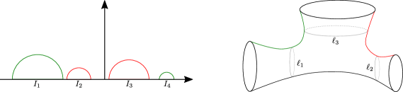
Figure 5. The right-hand side illustrates the three-funneled surface with boundary lengths $\ell_{1},\ell_{2},\ell_{3}$ embedded (non-isometrically) into three-dimensional Euclidean space. Highlighted in red and green is the Poincaré section (projected onto the surface) corresponding to the fundamental domain on the left.

5.3.2. Funneled torus

Our second family of surfaces is also well-known in the literature. Generators are given by

$$\begin{split}g_{1}&\mathrel{\mathop{:}\!\!=}\begin{pmatrix}\exp(\ell_{1}/2)&0\\ 0&\exp(-\ell_{1}/2)\end{pmatrix}\leavevmode\nobreak\ ,\\ g_{2}&\mathrel{\mathop{:}\!\!=}\begin{pmatrix}\cosh(\ell_{2}/2)-\cos(\varphi)\sinh(\ell_{2}/2)&\sin^{2}(\varphi)\sinh(\ell_{2}/2)\\ \sinh(\ell_{2}/2)&\cosh(\ell_{2}/2)+\cos(\varphi)\sinh(\ell_{2}/2)\end{pmatrix}\leavevmode\nobreak\ ,\end{split}$$

where again three parameters $\ell_{1},\ell_{2}$, and $\varphi$ are needed to specify a concrete member. Geometrically they describe the lengths of two closed geodesics on the surface and the angle between them. Obviously the generator $g_{1}$ contains the boundary point $\infty$ in its fundamental interval which makes it inaccessible for our algorithm because we use the fundamental intervals directly as coordinates of the Poincaré section. Conjugating the generators by a simple rotation yields a new pair $\widetilde{g}_{1}$ and $\widetilde{g}_{2}$ of generators which do not suffer from this problem. It turns out that $\pi/8$ is a particularly handy value in the maximally symmetric case $\ell_{1}=\ell_{2}$ and $\varphi=\pi/2$ as it leads to a very symmetric arrangement of fundamental circles (see also [BPSW20, Section 5.3] where the boundary point $\infty$ must be rotated outside of the fundamental intervals for somewhat similar reasons). In this case the conjugated generators are of the explicit form

$$\begin{split}\widetilde{g}_{1}&\mathrel{\mathop{:}\!\!=}\begin{pmatrix}\cosh(\ell/2)+\sinh(\ell/2)/\sqrt{2}&\sinh(\ell/2)/\sqrt{2}\\ \sinh(\ell/2)/\sqrt{2}&\cosh(\ell/2)-\sinh(\ell/2)/\sqrt{2}\end{pmatrix}\\ \widetilde{g}_{2}&\mathrel{\mathop{:}\!\!=}\begin{pmatrix}\cosh(\ell/2)-\sinh(\ell/2)/\sqrt{2}&\sinh(\ell/2)/\sqrt{2}\\ \sinh(\ell/2)/\sqrt{2}&\cosh(\ell/2)+\sinh(\ell/2)/\sqrt{2}\end{pmatrix}\leavevmode\nobreak\ .\end{split}$$

Again we adopt the same notation as in [Bor14] and denote the funneled tori generated by $\widetilde{g}_{1}$ and $\widetilde{g}_{2}$ by $Y(\ell_{1},\ell_{2},\varphi)$.

The generators $\widetilde{g}_{1}$ and $\widetilde{g}_{2}$ again admit a realization of Klein’s four-group as their symmetry group. Concrete symmetries are given by the Möbius transformations induced via

$$\sigma_{1}=\begin{pmatrix}0&1\\ 1&0\end{pmatrix},\qquad\sigma_{2}=\begin{pmatrix}0&1\\ -1&0\end{pmatrix}\leavevmode\nobreak\ ,$$

with their action on the symbols being the same as in (24). One can easily verify these relations by elementary matrix calculations of the type $\sigma_{1}\widetilde{g}_{1}\sigma_{1}^{-1}=\widetilde{g}_{2}$. The character table thus coincides with the one given above in Table 1.

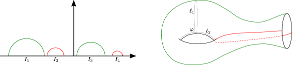
Figure 6. Here the right-hand side illustrates the funneled torus with parameters $\ell_{1},\ell_{2},\phi$ embedded (non-isometrically) into three-dimensional Euclidean space. Highlighted in red and green is the Poincaré section (projected onto the surface) corresponding to the fundamental domain on the left.

6. Numerical Results

This final section finishes the present paper by presenting some numerical calculations which were obtained with the tools developed up to this point. We begin with a comparison of convergence rates of invariant Ruelle distributions depending on the particular symmetry group used for a given surface.

Remark 6.1.

To do this we still require a practically feasible approach for the calculation of residues of $Z_{f}(\lambda)$. If one can calculate the function $Z_{f}(\lambda)$ efficiently for a large number of support points $\lambda\in\mathbb{C}$, i.e. on large arrays, then it would be possible to calculate its residue at $\lambda_{0}$ very generically via the classical integral formula

$$\underset{\lambda=\lambda_{0}}{\mathrm{Res}}\left[Z_{f}(\lambda)\right]=\frac{1}{2\pi\mathrm{i}}\int_{C}Z_{f}(\lambda)\leavevmode\nobreak\ \mathrm{d}\lambda\leavevmode\nobreak\ ,$$

where a convenient choice for the contour $C$ could e.g. be a sufficiently small rectangle with $\lambda_{0}$ at its center. This integral can then be evaluated using numerical quadrature methods.

If a large number of function evaluations is too computationally expensive then the following well-known formula offers an alternative:

$$\underset{\lambda=\lambda_{0}}{\mathrm{Res}}\left[Z_{f}(\lambda)\right]=\frac{1}{(N-1)!}\lim_{\lambda\rightarrow\lambda_{0}}\left(\frac{\mathrm{d}}{\mathrm{d}\lambda}\right)^{N-1}\left[(\lambda-\lambda_{0})^{N}Z_{f}(\lambda)\right]\leavevmode\nobreak\ ,$$

where $N$ denotes the order of the pole $\lambda_{0}$. If $N=1$, i.e. $\lambda_{0}$ is a simple pole, then this general formula takes a particularly simple shape and plugging in the logarithmic derivative of the dynamical determinant $d_{f}$ yields for the simple case

$$\underset{\lambda=\lambda_{0}}{\mathrm{Res}}\left[Z_{f}(\lambda)\right]=\frac{\partial_{\beta}d_{f}(\lambda_{0},1,0)}{\partial_{\lambda}d_{f}(\lambda_{0},1,0)}\leavevmode\nobreak\ .$$ (25)

This expression can be evaluated directly because calculation of $\partial_{\lambda}d_{f}$ requires only a straightforward modification of our algorithm for $d_{f}$ and $\partial_{\beta}d_{f}$. The numerics presented below feature only simple poles so we used (25) throughout our implementations.

Funneled Torus Experiments

The first system we consider is the funneled torus for the two cases of its full $4$-element Kleinian symmetry group as described in Section 5.3.2 and without any symmetry reduction. The quantum resonance spectrum for the concrete example $Y\left(10,10,\frac{\pi}{2}\right)$ was already obtained numerically by Borthwick [Bor14, Figure 11] by means of Selberg’s zeta function. In Figure 7 we recover this spectrum but now using the dynamical determinant $d_{f}$ with constant weight function $f$. This yields the Pollicott-Ruelle resonances of $Y\left(10,10,\frac{\pi}{2}\right)$ which by [GHW18] coincide with the quantum spectrum after a shift by $-1$. Compared with previous calculations of quantum resonances in the literature our numerics therefore illustrate this theorem about the relationship between classical and quantum resonances.

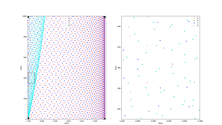
Figure 7. Resonances of the funneled torus $Y\left(10,10,\frac{\pi}{2}\right)$ calculated in the symmetry reduction by the Klein four-group. The right-hand side shows a zoom into a small region of the left-hand side plot. Notice how the representations labeled B and D split resonances of multiplicity two into pairs of resonances of multiplicity one. In particular this simplifies the formula for the calculation of invariant Ruelle distributions via residues as described above. The four resonances marked by black stars in the left plot were used for investigations of Ruelle distributions below.

We begin by investigating in more detail the first resonance of $Y(10,10,\pi/2)$ which is located at $\delta-1\approx-0.8847$ with $\delta$ the Hausdorff dimension of the limit set. The result of numerically calculating $t^{\Sigma}_{\lambda_{0},\sigma}$ is shown in Figure 9 as plots of three different quantities: The left-most plot shows the real part of the distribution which gets complemented by the imaginary part in the middle. The invariant Ruelle distribution associated with the first resonance coincides with the Bowen-Margulis measure so it should be expected that the numerical approximation is real-valued and positive which is exactly the case in the shown plot. The right-most coordinate square features a combination of real and imaginary parts: There the complex argument is indicated through the color of the peaks and the absolute value of $t^{\Sigma}_{\lambda_{0},\sigma}$ was encoded as the lightness of the particular color. The mapping of colors to complex arguments is simply given by the angle on the standard color wheel in the HSB/HSL encoding of RGB shifted by $\pi$, i.e. light blue corresponds to an argument of $0$ while red corresponds to $\pi$ (see Figure 8). From this illustration it is immediately clear that the distribution is remarkably homogeneous within each square $I_{i}\times I_{j}$ of the coordinate domain parameterizing the Poincaré section.

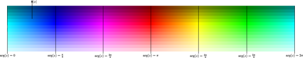
Figure 8. Sketch of how complex arguments $\mathrm{arg}(z)$ map to different colors in the phase plots above. The absolute value $|z|$ maps to the lightness of the color as a second dimension with darker colors corresponding to higher values of $|z|$.

Figure 9. Invariant Ruelle distribution $t^{\Sigma}_{\lambda_{0},\sigma}$ on the canonical Poincaré section $\Sigma$ of the funneled torus $Y(10,10,\pi/2)$ associated with the first resonance $\lambda_{0}\approx-0.8847$. This figure uses the width $\sigma=10^{-3}$ and $n_{\mathrm{max}}=5$ summands in the cycle expansion of the dynamical determinant $d_{f}$. The fundamental intervals $I_{i}$ which parameterize the section are ordered as qualitatively shown in Figure 6 The left and middle columns show the real and imaginary parts of the distribution. The right column encodes both real and imaginary parts by using the complex argument to determine the color (as an angle on the color wheel) and the absolute value to provide the lightness.

Next we consider additional resonances from Figure 7 under the aspect of how well the associated distributions converge in practice. It is reasonable to expect that the outer edges of the square $[-1,\delta-1]+[0,1000]\mathrm{i}$ of the complex plane where resonances were calculated should correspond to the best respectively worst rates of convergence. To increase the resolution of the distribution the plots were additionally restricted to coordinates within strictly smaller intervals

$$(\widetilde{I}_{2}\cup\widetilde{I}_{3}\cup\widetilde{I}_{3})\times(\widetilde{I}_{1}\cup\widetilde{I}_{2})\leavevmode\nobreak\ ,\qquad\widetilde{I}_{i}\subset I_{i}\leavevmode\nobreak\ ,$$

where the location of the new intervals within the original fundamental domain is illustrated in Figure 10.

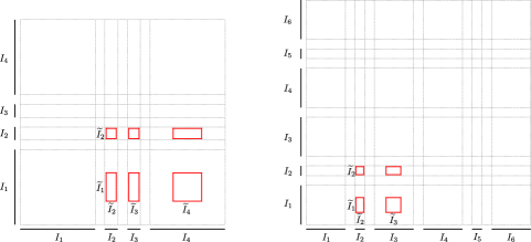
Figure 10. Location and relative size of the refined coordinate domains $\widetilde{I}_{i}\subset I_{i}$ compared to the original fundamental intervals of the funneled torus $X(10,10,\pi/2)$ (left) and the three-funneled surface $X(12,12,12)$ (right).

This very basic domain refinement already reduces the amount of redundancy in the resulting plots significantly by excluding large areas where the distributions vanish and exploiting the internal symmetries of the distributions as prominently visible in Figure 9.

The resulting plots for a collection of four resonances are depicted in Figure 11: Here the columns correspond to the same resonance whereas the rows share a common cutoff order $n_{\mathrm{max}}$, i.e. the number of summands used in the cycle expansion. From this figure we see that even the distribution associated with the resonance $\lambda_{0}\approx-0.9999+992.4\mathrm{i}$ in the upper left of the considered resonance domain converges nicely already at $n_{\mathrm{max}}=3$.

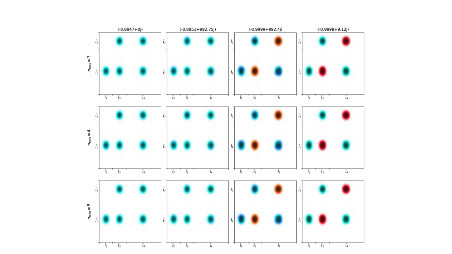
Figure 11. Fully symmetry reduced invariant Ruelle distributions $t^{\Sigma}_{\lambda_{0},\sigma}$ on the canonical Poincaré section $\Sigma$ of the funneled torus $Y(10,10,\pi/2)$ evaluated at four different choices of resonance $\lambda_{0}$ (marked in Figure 7) with $\sigma=10^{-3}$. The three different rows show the numerical results of using (from top to bottom) $n_{\mathrm{max}}\in\{3,4,5\}$ summands in the cycle expansion. Following along any of the four columns shows that the presented plots have converged rather well already at $n_{\mathrm{max}}=3$. Due to symmetries in the distributions as visible in Figure 9 it suffices to consider as the coordinate domain the refined subset $(\widetilde{I}_{2}\cup\widetilde{I}_{3}\cup\widetilde{I}_{4})\times(\widetilde{I}_{1}\cup\widetilde{I}_{2})$ of Figure 10.

One particularly noteworthy feature of these plots is the large degree of similarity between the first and second columns both with respect to the absolute value as well as the complex argument. An explanation for this qualitative agreement might be the fact that both associated resonances are located near the global spectral gap at

$$\mathrm{Re}(\lambda)=\delta-1$$

and a first conjecture could be that recurrence to this gap which was observed in previous investigations of quantum resonances on convex-cocompact hyperbolic surfaces is related to properties of resonant states.

By analogy with the application of cycle expansion to resonances it is straightforward to conjecture that symmetry reduction should improve the rate of convergence of invariant Ruelle distributions even for the (rather small) Klein four-group used with $Y(10,10,\pi/2)$. To support this claim the experiment above was repeated with the trivial one-element symmetry group $\{e\}$. Once converged our numerical results should be independent from the symmetry group used: While the approximation $t^{\Sigma}_{\lambda_{0},\sigma}$ does contain a symmetric version of the Gaussian test functions this should not matter due to the global invariant Ruelle distribution also being invariant with respect to the full symmetry group of the surface.

The resulting plots in Figure 12 do indeed coincide with those of Figure 11 while at the same time exhibiting worse convergence properties: The distribution at $\lambda_{0}\approx-0.9999+992.4\mathrm{i}$ has not converged until $n_{\mathrm{max}}=7$. While not visible in the figure itself this worsened convergence rate also shows up for the other three resonances as can be seen by considering the relative errors of order $N$

$$\frac{\big{|}d_{N}^{\chi}(\lambda_{0},0)\big{|}}{\big{|}1+\sum_{n=1}^{N}d_{n}^{\chi}(\lambda_{0},0)\big{|}}\leavevmode\nobreak\ .$$

Note that these quantities are still functions of the coordinates $(x_{-},x_{+})$ due to their dependence on the particular weight function used. Two straightforward ways to obtain scalar measures of convergence quality are given by either averaging with respect to $(x_{-},x_{+})$ over the whole coordinate domain of the Poincaré section or to take the maximum norm. We consistently tracked both variants for all our experiments and it turned out that in all cases they differed at most by one order of magnitude.

As an example we observed for the resonance $\lambda_{0}\approx-0.9998+9.12\mathrm{i}$ errors of $3.38\cdot 10^{-8}$ and $1.94\cdot 10^{-8}$ after $n=4$ iterations with symmetry reduction but $3.2\cdot 10^{-4}$ as well as $9.82\cdot 10^{-5}$ after $n_{\mathrm{max}}=6$ iterations without reduction. This discrepancy becomes slightly smaller near the first resonances as $\lambda_{0}=\delta-1$ universally shows the best convergence behavior.

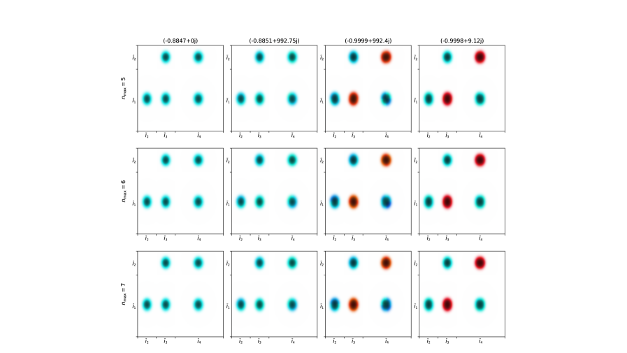
Figure 12. Analogous plots of $t^{\Sigma}_{\lambda_{0},\sigma}$ for $\Sigma$ the canonical Poincaré section of the funneled torus $Y(10,10,\pi/2)$ and $\sigma=10^{-3}$ as in Figure 11 but now symmetry reduced by the trivial (one-element) group $\{e\}$. The invariant Ruelle distribution is itself invariant under the finite symmetry group of the surface so these plots should (and do) coincide with those of Figure 11 apart from the significantly higher cutoff $n_{\mathrm{max}}=7$ required for convergence of the cycle expansion (especially in the third column).

Three-funneled Surface Experiments

Next we conduct the analogous experiments for the three-funneled surface $X(12,12,12)$. The symmetry group of the standard set of generators was identified as the Klein four-group in Section 5.3.1 but this is actually not the full group of symmetries: In [BW16] it was demonstrated how a flow-adapted representation of $X(\ell,\ell,\ell)$ yields a strictly larger symmetry group thereby unlocking the full power of symmetry reduction for this class of surfaces. Without going into the details we state that this technique can be adapted to the dynamical determinants considered here so we may calculate with straightforward adaptations of the techniques described above invariant Ruelle distributions for the flow-adapted three-funnel surfaces. For a comprehensive description of the theoretical background refer to the first author’s PhD thesis [Sch23].

Remark 6.2.

Geometrically the flow-adapted representation is defined by gluing two copies of hyperbolic space with three disjoint halfplanes removed, see Figure 13. This corresponds to a canonical Poincaré section which is far more symmetric compared to the Schottky representation of three-funneled surfaces.

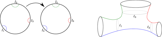
Figure 13. Illustration of the gluing of two copies of the Poincaré disc $\mathbb{D}$ (left) along the colored circles resulting in a three-funnel surface (right). The Poincaré section resulting from this gluing treats the three seams along the funnels equally.

Figure 14. Resonances of the three-funnel surface $X(12,12,12)$ calculated in the full symmetry reduction of its flow-adapted representation. Due to the high degree of symmetry of the surface four very distinct resonance chains are visible. The right-hand side displays a zoom into the region where all four chains cross. It clearly shows how every chain belongs to a pair of representations which appear along the chain in alternating fashion. Again the four resonances considered below were marked with black stars.

As a first step we again use the dynamical determinant to calculate the Pollicott-Ruelle resonances of this Schottky surface, see Figure 14. As expected from the quantum-classical correspondence this recovers the (shifted) quantum mechanical resonances already calculated in [Bor14, Figure 6] as well as the symmetry behavior of individual resonances as determined in [BW16, Figure 8]. Note that the full symmetry group of the flow-adapted three-funneled surfaces exhibits six irreducible unitary representations resulting in six different classes of resonances. One also prominently observes the same resonant chains already studied in [BW16].

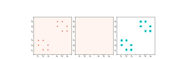
Figure 15. Invariant Ruelle distribution $t^{\Sigma}_{\lambda_{0},\sigma}$ on the canonical Poincaré section $\Sigma$ of the three-funnel surface $X(12,12,12)$ associated with the first resonance $\lambda_{0}\approx 0.8845$. This figure uses the width $\sigma=10^{-2}$ and $n_{\mathrm{max}}=5$ summands in the cycle expansion of the dynamical determinant $d_{f}$. Notice how the finite symmetry group of the function system and the surface itself still shows up in the distribution. The plots show (from left to right) real part, imaginary part, and argument/absolute value encoding of the distribution similar to Figure 9.

With these first resonances available to us we can proceed very similarly to the funneled torus case. Again we compute the smoothed invariant Ruelle distribution $t^{\Sigma}_{\lambda_{0},\sigma}$ on the canonical Poincaré section of the flow-adapted system associated with the first resonance $\lambda_{0}=\delta-1\approx-0.8845$. The resulting plot is shown in Figure 15. Again the plot possesses the theoretically known properties of being real-valued and positive, as well as showing a clear symmetry with respect to the finite symmetry group of the underlying function system.

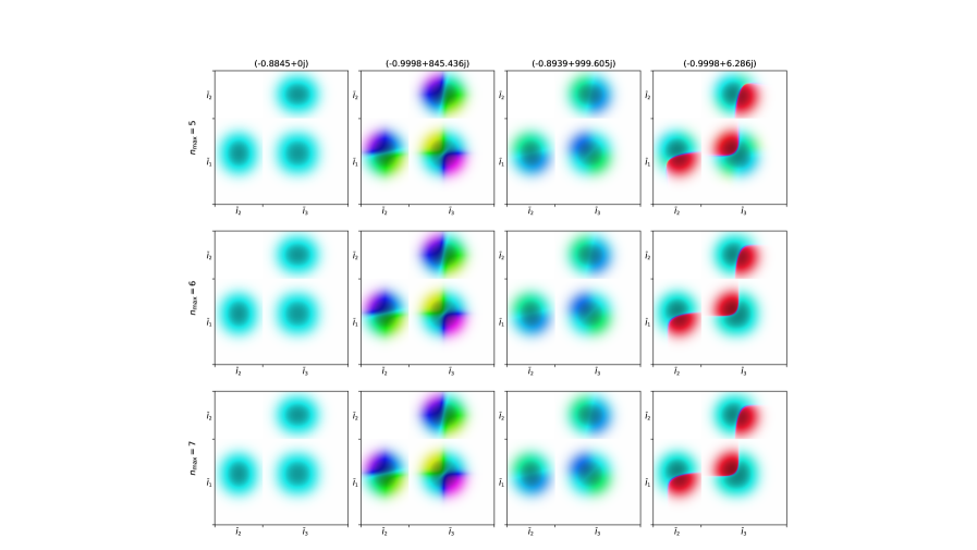
Figure 16. Fully symmetry reduced invariant Ruelle distributions $t^{\Sigma}_{\lambda_{0},\sigma}$ on the canonical Poincaré section $\Sigma$ of the flow-adapted three-funnel surface $X(12,12,12)$ evaluated at four different choices of resonance $\lambda_{0}$ with $\sigma=10^{-2}$ and plotted as phase-lightness. The three different rows show the numerical results of using (from top to bottom) $n_{\mathrm{max}}\in\{5,6,7\}$ summands in the cycle expansion. Following along any of the four columns shows that the presented plots have converged rather well already at $n_{\mathrm{max}}=5$. Due to symmetries in the distributions as shown in Figure 15 it again suffices to consider as the coordinate domain refined subsets $(\widetilde{I}_{2}\cup\widetilde{I}_{3})\times(\widetilde{I}_{1}\cup\widetilde{I}_{2})$ which are shown in Figure 10.

As a next step we support the observations made above for the funneled torus with analogous experiments for $X(12,12,12)$: Figure 16 contains plots of invariant Ruelle distributions for a set of four different resonances located roughly on the corners of the resonance plot calculated in full symmetry reduction and the comparison with Figure 17 which uses the trivial symmetry group $\{e\}$ shows again the great benefit of symmetry reduction when it comes to the practical rate of convergence, i.e. the required number of summands in the cycle expansion. Comparing the funneled torus with the three-funneled surfaces also reveals that the former requires the determination of more geodesic lengths and orbit integrals to achieve the same relative errors as the latter even though this difference is not quite as significant as the difference between reduced and non-reduced calculations.

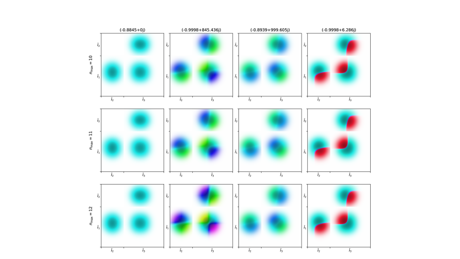
Figure 17. Analogous plots of $t^{\Sigma}_{\lambda_{0},\sigma}$ for $\Sigma$ the canonical Poincaré section of the flow-adapted representation of $X(12,12,12)$ and $\sigma=10^{-2}$ as in Figure 16 but here the trivial symmetry group $\{e\}$ was used. Again the distributions are in close qualitative agreement with those in Figure 16 but convergence required significantly more terms in the cycle expansion as illustrated by the obvious lack of convergence in the second column.

We note that the first and third columns of Figure 16 which correspond to the first resonance and the next resonance which is closest to the global spectral gap show far less similarity than observed for the funneled torus in the first and second columns of Figure 11. But this is simply due to the fact that we can follow the resonance chain corresponding to the representations II1/II2 further to the right and the resonance on this chain which is closest to the global gap actually turns out to be located quite a bit higher at $\lambda_{0}\approx-0.8845+1269.2\mathrm{i}$. In Figure 18 both this resonance chain as well as the invariant Ruelle distribution corresponding to the chain maximum were plotted. The distribution clearly supports the hypothesis developed for the funneled torus namely that Ruelle distributions associated with resonances near the global spectral gap should show high qualitative agreement with the one attached to the first resonance.

The experiment in Figure 18 also supports another trend with respect to convergence rates: The practical rates are much more sensitive to the real than the imaginary parts of the associated resonance. Even at the rather high imaginary part of $\approx 1269.2$ the distributions convergence rapidly in full symmetry reduction with relative errors of magnitude $\approx 10^{-6}$ after only $n_{\mathrm{max}}=4$ iterations. This behavior is rather promising for future experiments involving resonance chains near the global spectral gap!

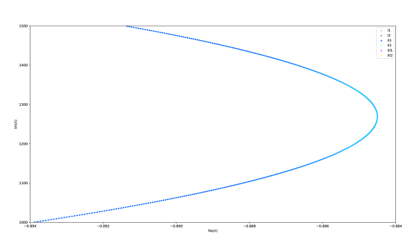
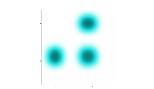
Figure 18. Additional resonances along the chain of II1/II2 resonances already starting in Figure 14 (top plot) together with the invariant Ruelle distribution at the chain resonance $\lambda_{0}\approx-0.8845+1269.20\mathrm{i}$ closest to the global spectral gap $\mathrm{Re}(\lambda)=\delta-1\approx-0.8845$ (bottom plot). The comparison with the first column in Figure 16 which uses the same width $\sigma=10^{-2}$ shows near perfect qualitative agreement supporting the analogous observation made for the funneled torus above.

The preceding examples should clearly justify the statements made in Section 5 – symmetry reduction does indeed improve the convergence properties of invariant Ruelle distributions drastically. Furthermore the example of three-funneled surfaces shows that one should use the largest available symmetry group for a given Schottky surface whenever possible to take maximal advantage of the symmetries of the surface. Finally refinement of the coordinate domain parameterizing the Poincaré section is vital if we want to be able to distinguish the relevant features of the calculated distributions with sufficient resolution. For systematic experiments in a regime where the fractal limit set is resolved beyond the first level our ad-hoc procedure can easily be augmented: After an application of group elements corresponding to a certain word length the initial fundamental intervals have multiplied according to the given word length but the resulting intervals are also contracted. One can now choose a subset of these contracted intervals which are representative for the distribution with respect to the symmetry group of the surface. This effectively increases the resolution of the numerical approximations without requiring a larger grid of support points on the coordinate domains.

Additional Three-funneled Surface Plots

Even though already restricted to two-dimensional quantities our approximations $t^{\Sigma}_{\lambda_{0},\sigma}$ of invariant Ruelle distributions are still complex-valued functions on a two-dimensional domain effectively making them four-dimensional quantities. Any visualization will necessarily have to emphasize certain aspects of these distributions over others. The particular kind of phase-lightness plots used for illustration above showed nicely the qualitative behavior in terms of phase but the variations in absolute value are not as distinct. The following plots in Figure 19 therefore emphasize this latter aspect by showing the analogue of Figure 16 but as a plot of the absolute value alone.

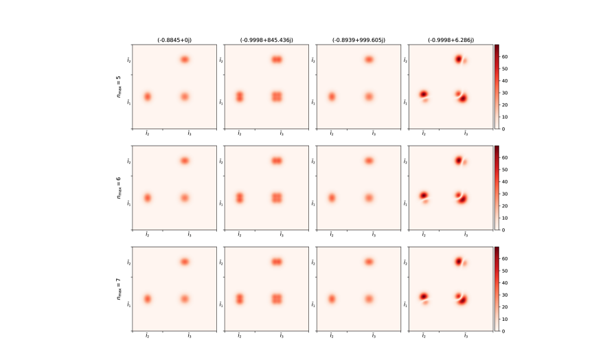
Figure 19. Absolute values of fully symmetry reduced invariant Ruelle distributions $t^{\Sigma}_{\lambda_{0},\sigma}$ on the canonical Poincaré section $\Sigma$ of the flow-adapted three-funnel surface $X(12,12,12)$ evaluated at four different choices of resonance $\lambda_{0}$ with $\sigma=10^{-2}$. Again the different rows show the numerical results of using (from top to bottom) $n_{\mathrm{max}}\in\{5,6,7\}$ summands in the cycle expansion. Following along any of the four columns shows that the presented plots have converged rather well already at $n_{\mathrm{max}}=5$. To increase resolution the coordinates $(x_{-},x_{+})$ were again restricted to the refined rectangles $(\widetilde{I}_{2}\cup\widetilde{I}_{3})\times(\widetilde{I}_{1}\cup\widetilde{I}_{2})$ of Figure 10.

As second important facet not yet discussed is the dependence of the qualitative features as well as the convergence behavior of $t^{\Sigma}_{\lambda_{0},\sigma}$ on the Gaussian width $\sigma$. We therefore plotted the distributions using $\sigma=10^{-2}$ in Figure 19 again for different values of $n_{\mathrm{max}}$ to compare them with the results for $\sigma=7\cdot 10^{-3}$ in the subsequent Figure 20.

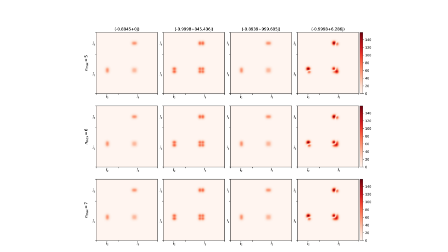
Figure 20. Similar to Figure 19 but now with $\sigma=7\cdot 10^{-3}$. Due to the smaller value of $\sigma$ the resolution of the trapped set has become significantly better especially in columns two and four but at the expense of the rate of convergence: Now the right-most column changes noticeably between $n_{\mathrm{max}}=5$ and $n_{\mathrm{max}}=6$.

The comparison shows how decreasing the width $\sigma$ brings out additional features in the distributions in particular the convergence of their supports towards the fractal limit set of the underlying surface. This comes at the expense of decreased convergence speed, though, as illustrated by the fourth column in Figure 20. The benefits of symmetry reduction should therefore be even more pronounced when combined with experiments of the regime $\sigma\rightarrow 0$ for distributions associated with resonances far from the global spectral gap.

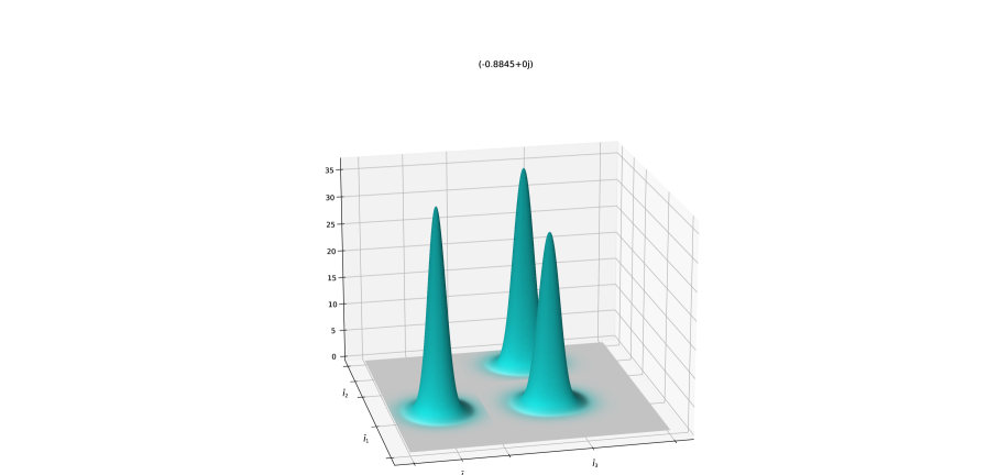
Figure 21. Three-dimensional representation of the invariant Ruelle distribution for the three-funneled surface $X(12,12,12)$ on the canonical Poincaré section of the flow-adapted system and with Gaussian width $\sigma=10^{-2}$ associated to the first resonance $\lambda_{0}\approx-0.8845$. The absolute value of the distribution determines the height of the surface whereas the colors indicate the position of the complex argument on the unit circle. This effectively combines the presentation in Figures 16 and 19 emphasizing nicely the homogeneity of the first invariant Ruelle distribution.

We finish this first numerical tour of invariant Ruelle distributions by considering a third technique to illustrate these that combines the phase-focused and absolute-valued focused approaches taken so far: By increasing the dimension of the plots themselves we can map the absolute value to the height of a surface in three-dimensional space and simultaneously color this surface according to the phase (argument) of the complex values. The resulting plot for the first resonance of $X(12,12,12)$ is shown in Figure 21. While visually more complex due to its three-dimensional nature it does illustrate the distribution in quite an intuitive manner and the high homogeneity present in the first invariant Ruelle distribution is immediately apparent.

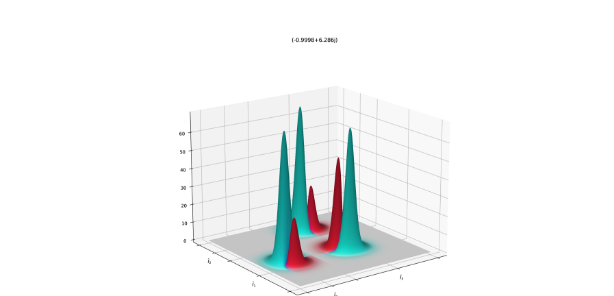
Figure 22. Analogous plot as in Figure 21 but for the resonance $\lambda_{0}\approx-0.9998+6.286\mathrm{i}$ and again the same Gaussian width $\sigma=10^{-2}$. The three-dimensional plot brings out the splitting of each peak into two sub-peaks of distinctly different phases better than the corresponding absolute value plot in the fourth column of Figure 19.

The plots contained in Figures 22 and 23 show the three-dimensional representation of a different resonance already considered in Figures 19 and 20 for the widths $\sigma=10^{-2}$ and $\sigma=7\cdot 10^{-3}$. The splitting of larger peaks into sub-peaks supported on a neighborhood of the limit set is brought out very clearly as well as the very distinct phases corresponding to different sub-peaks. Decreasing $\sigma$ emphasizes these features further but is less necessary than for the absolute value plots considered previously.

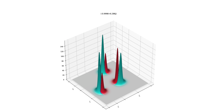
Figure 23. Analogous plot as in Figure 22 for the same resonance $\lambda_{0}\approx-0.9998+6.286\mathrm{i}$ but a refined Gaussian width of $\sigma=7\cdot 10^{-3}$. Even this slight decrease in $\sigma$ already increases the resolution of distinct sub-peaks with rather prominent differences in phase by quite a margin.

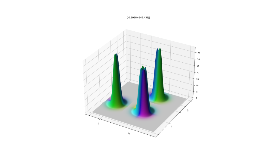
Figure 24. Analogous plot as in Figure 21 but for the resonance $\lambda_{0}\approx-0.9998+845.436\mathrm{i}$ and again width $\sigma=10^{-2}$. The splitting into pairs and quadruples of sub-peaks is significantly easier to distinguish than in the corresponding absolute value plot shown in the second column of Figure 19.

Finally the same experiment was repeated in Figures 24 and 25 with a second resonance of $X(12,12,12)$ where one of the major peaks even splits into four sub-peaks already at $\sigma=10^{-2}$ and more clearly at $\sigma=7\cdot 10^{-3}$.

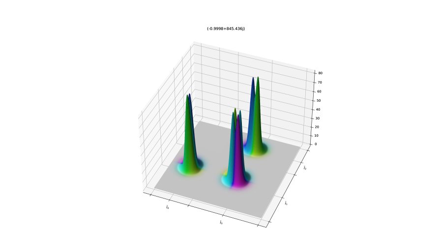
Figure 25. Analogous plot as in Figure 24 associated with the same resonance $\lambda_{0}\approx-0.9998+845.436\mathrm{i}$ but for a refined Gaussian width of $\sigma=7\cdot 10^{-3}$. Note how both the pairs and the quadruple of peaks are visually more distinct due to the (slight) decrease in $\sigma$.

In summary we observe that the expected limiting behavior where for $\sigma\rightarrow 0$ the numerically calculated distributions should converge to quantities supported on the (fractal) limit set can indeed be found in our concrete experiments. We also observed that there are practical limits to the lower bound on $\sigma$ mostly dictated by an inverse relationship between the value of $\sigma$ and the required maximal number of summands $n_{\mathrm{max}}$ in the cycle expansion of the dynamical determinant. Here symmetry reduction begins to show its large potential despite the fact that only a few first experiments were conducted. But even with decently sized values of $\sigma$ the three-dimensional representations of $t^{\Sigma}_{\lambda_{0},\sigma}$ exhibit a number of interesting features that should provide further insights into the structure of invariant Ruelle distributions, resonant states, and their associated resonances.

Remark 6.3.

Additional numerical experiments including in particular animations are being prepared and will be included in future versions of this article as well as the first author’s PhD thesis [Sch23].

7. Outlook

In the present article we derived and implemented an algorithm for the practical numerical computation of invariant Ruelle distributions. This opens the possibility to perform a large number of different numerical experiments on which an outlook was already given in the final Section 6. More systematic investigations will be conducted in the future to fully leverage the tools developed here.

Besides such experiments another interesting perspective would be to transfer the methods of [BPSW20] for the numerical calculation of Fredholm determinants to our (weighted) dynamical determinants $d_{f}$. These techniques showed very promising improvements over the computational cost and convergence of cycle expansions in the resonance case and it is expected that similar improvements are possible with minor adaptations in the case of invariant Ruelle distributions.

Appendix A Fredholm Determinants

In this appendix we summarize some facts regarding functional analysis in general and Fredholm determinants in particular. We include this appendix to make the present paper and specifically our proofs more self-contained. All of the following material is quite standard and the proofs can be found in e.g. [Bor16, Appendix A.4] or the monograph [Sim05, Chap. 1 & 3].

Definition A.1.

Let $T:\mathcal{H}_{1}\rightarrow\mathcal{H}_{2}$ be a compact operator between the Hilbert spaces $\mathcal{H}_{1}$ and $\mathcal{H}_{2}$. The square roots of the eigenvalues of the self-adjoint operator $TT^{*}$ are called singular values of $T$ and denoted by

$$\mu_{1}(T)\geq\mu_{2}(T)\geq\ldots\longrightarrow 0\leavevmode\nobreak\ .$$

If $\mathcal{H}_{1}=\mathcal{H}_{2}$ then $T$ is called trace-class in case $\sum_{i=1}^{\infty}\mu_{i}(T)<\infty$ holds.

For the next definition we denote, analogously to the singular values, the sequence of eigenvalues of $T$ ordered w.r.t. decreasing absolute value and repeated according to their multiplicity by $\lambda_{1}(T),\lambda_{2}(T),\ldots$.

Definition A.2.

Let $T:\mathcal{H}\rightarrow\mathcal{H}$ be a trace-class operator on the Hilbert space $\mathcal{H}$. Then the Fredholm determinant of $T$ is defined as

$$\mathrm{det}\left(\mathrm{id}-zT\right)\mathrel{\mathop{:}\!\!=}\prod_{i=1}^{\infty}\left(1+z\lambda_{i}(T)\right)\leavevmode\nobreak\ ,$$ (26)

and converges for any $z\in\mathbb{C}$.

Theorem A.3.

Let $T:\mathcal{H}\rightarrow\mathcal{H}$ be a compact operator on the Hilbert space $\mathcal{H}$ and denote by $\bigwedge^{i}T$ the $i$-th exterior power of $T$. Then the Fredholm determinant can be calculated via

$$\mathrm{det}\left(\mathrm{id}-zT\right)=\sum_{i=0}^{\infty}z^{i}\cdot\mathrm{Tr}\left(\bigwedge^{i}T\right)\leavevmode\nobreak\ ,$$

where the trace of $T$ may be defined as $\mathrm{Tr}(T)\mathrel{\mathop{:}\!\!=}\sum_{i=1}^{\infty}\lambda_{j}(T)$.

Combining this theorem with the inequality

$$\sum_{j=1}^{\infty}|\lambda_{j}(T)|\leq\sum_{j=1}^{\infty}\mu_{j}(T)$$

one can now prove the analyticity of the Fredholm determinant in the $z$-variable: The trace which is its $i$-th coefficient in the Taylor expansion about $z=0$ can be bounded by

$$\sum_{j_{1}<\ldots<j_{i}}\mu_{j_{1}}(T)\cdot\ldots\cdot\mu_{j_{i}}(T)\leq\frac{1}{k!}\left(\sum_{j=1}^{\infty}\mu_{j}(T)\right)^{i}\leavevmode\nobreak\ ,$$

because $\left(\bigwedge^{i}T\right)\left(\bigwedge^{i}T\right)^{*}=\bigwedge^{i}\left(TT^{*}\right)$. But this already finishes the proof due to $T$ being trace-class.

We end this appendix by stating two well-known estimates regarding singular values:

Theorem A.4 (Min-Max-Theorem).

Let $T:\mathcal{H}\rightarrow\mathcal{H}$ be a compact operator on the Hilbert space $\mathcal{H}$. Then the $n$-th singular value of $T$ satisfies

$$\mu_{n}(T)=\min_{\begin{subarray}{c}V\subseteq\mathcal{H}\\ \dim(V)=n-1\end{subarray}}\max_{\varphi\in V^{\bot}}\frac{\Arrowvert T\varphi\Arrowvert}{\Arrowvert\varphi\Arrowvert}\leavevmode\nobreak\ .$$

Theorem A.5 (Fan Inequality).

Let compact operators $S,T:\mathcal{H}\rightarrow\mathcal{H}$ on the Hilbert space $\mathcal{H}$ be given. Then the singular values of $S+T$ satisfy

$$\mu_{i+j-1}(S+T)\leq\mu_{i}(S)+\mu_{j}(T)\leavevmode\nobreak\ .$$

References

- [AZ07] N. Anantharaman and S. Zelditch, Patterson–Sullivan distributions and quantum ergodicity, Annales Henri Poincaré 8 (2007), no. 2, 361–426.
- [Bal18] V. Baladi, Dynamical Zeta Functions and Dynamical Determinants for Hyperbolic Maps, 1st ed., Ergebnisse der Mathematik und ihrer Grenzgebiete. 3. Folge / A Series of Modern Surveys in Mathematics, Springer, 2018.
- [BKL02] M. Blank, G. Keller, and C. Liverani, Ruelle–Perron–Frobenius spectrum for Anosov maps, Nonlinearity 15 (2002), no. 6, 1905–1973.
- [Bor14] D. Borthwick, Distribution of resonances for hyperbolic surfaces, Experimental Mathematics 23 (2014), no. 1, 25–45.
- [Bor16] by same author, Spectral Theory of Infinite-Area Hyperbolic Surfaces, 2nd ed., Progress in Mathematics, Birkhäuser, 2016.
- [BPSW20] O. F. Bandtlow, A. Pohl, T. Schick, and A. Weiße, Numerical resonances for Schottky surfaces via Lagrange–Chebyshev approximation, Stochastics and Dynamics (2020), 2140005.
- [BSW22] S. Barkhofen, P. Schütte, and T. Weich, Semiclassical formulae for Wigner distributions, Journal of Physics A: Mathematical and Theoretical 55 (2022), no. 24, 20.
- [BW16] D. Borthwick and T. Weich, Symmetry reduction of holomorphic iterated function schemes and factorization of Selberg zeta functions, Journal of Spectral Theory 6 (2016), no. 2, 267–329.
- [CDDP22] Mihajlo Cekić, Benjamin Delarue, Semyon Dyatlov, and Gabriel P. Paternain, The Ruelle zeta function at zero for nearly hyperbolic 3-manifolds, Invent. Math. 229 (2022), no. 1, 303–394 (English).
- [CE89] P. Cvitanović and B. Eckhardt, Periodic-orbit quantization of chaotic systems, Physical review letters 63 (1989), no. 8, 823–826.
- [Com74] L. Comtet, Advanced Combinatorics, 1st revised and enlarged ed., Springer Dordrecht, 1974.
- [Dal11] F. Dal’Bo, Geodesic and Horocyclic Trajectories, 1st ed., Universitext, Springer London, 2011.
- [DG16] S. Dyatlov and C. Guillarmou, Pollicott–Ruelle Resonances for Open Systems, Annales Henri Poincaré 17 (2016), no. 11, 3089–3146.
- [DG21] Nguyen-Thi Dang and Olivier Glorieux, Topological mixing of Weyl chamber flows, Ergodic Theory and Dynamical Systems 41 (2021), no. 5, 1342–1368.
- [DGRS20] Nguyen Viet Dang, Colin Guillarmou, Gabriel Rivière, and Shu Shen, The Fried conjecture in small dimensions, Invent. Math. 220 (2020), no. 2, 525–579 (English).
- [DSW21] B. Delarue, P. Schütte, and T. Weich, Resonances and Weighted Zeta Functions for Obstacle Scattering via Smooth Models, arXiv:2109.05907 (2021).
- [Dya19] Semyon Dyatlov, Improved fractal Weyl bounds for hyperbolic manifolds (with an appendix by David Borthwick, Semyon Dyatlov and Tobias Weich), J. Eur. Math. Soc. (JEMS) 21 (2019), no. 6, 1595–1639 (English).
- [DZ16] S. Dyatlov and M. Zworski, Dynamical zeta functions for Anosov flows via microlocal analysis, Annales de l’ENS 49 (2016), 543–577.
- [DZ17] Semyon Dyatlov and Maciej Zworski, Ruelle zeta function at zero for surfaces, Invent. Math. 210 (2017), no. 1, 211–229 (English).
- [DZ19] S. Dyatlov and M. Zworski, Mathematical theory of scattering resonances, 1st ed., Graduate Studies in Mathematics, vol. 200, American Mathematical Soc., 2019.
- [FH04] W. Fulton and J. Harris, Representation Theory – A First Course, 1st ed., Graduate Texts in Mathematics, Springer New York, NY, 2004.
- [FT23] Frédéric Faure and Masato Tsujii, Fractal weyl law for the ruelle spectrum of anosov flows, Annales Henri Lebesgue 6 (2023), 331–426.
- [GHW18] Colin Guillarmou, Joachim Hilgert, and Tobias Weich, Classical and quantum resonances for hyperbolic surfaces, Math. Ann. 370 (2018), 1231–1275.
- [GHW21] C. Guillarmou, J. Hilgert, and T. Weich, High frequency limits for invariant Ruelle densities, Annales Henri Lebesgue 4 (2021), 81–119.
- [GR89] Pierre Gaspard and Stuart A Rice, Scattering from a classically chaotic repellor, The Journal of Chemical Physics 90 (1989), no. 4, 2225–2241.
- [Hö03] L. Hörmander, The Analysis of Linear Partial Differential Operators I, 2nd ed., Classics in Mathematics, Springer Berlin, Heidelberg, 2003.
- [JP02] O. Jenkinson and M. Pollicott, Calculating Hausdorff dimension of Julia sets and Kleinian limit sets, American Journal of Mathematics 124 (2002), no. 3, 495–545.
- [KW20] Benjamin Küster and Tobias Weich, Pollicott-Ruelle resonant states and Betti numbers, Commun. Math. Phys. 378 (2020), no. 2, 917–941 (English).
- [Mas67] Bernard Maskit, A characterization of Schottky groups, Journal d’Analyse Mathématique 19 (1967), 227–230.
- [NZ15] S. Nonnenmacher and M. Zworski, Decay of correlations for normally hyperbolic trapping, Invent. math. 200 (2015), 345–438.
- [Pol85] Mark Pollicott, On the rate of mixing of Axiom A flows, Invent. Math. 81 (1985), 413–426.
- [PV19] Mark Pollicott and Polina Vytnova, Zeros of the Selberg zeta function for symmetric infinite area hyperbolic surfaces, Geom. Dedicata 201 (2019), 155–186 (English).
- [Rob03] Thomas Roblin, Ergodicity and equidistribution in negative curvature, Mém. Soc. Math. Fr., Nouv. Sér. 95 (2003), 96 (French).
- [Rue76] David Ruelle, Zeta-functions for expanding maps and Anosov flows, Invent. Math. 34 (1976), 231–242.
- [Rug92] H. H. Rugh, The correlation spectrum for hyperbolic analytic maps, Nonlinearity 5 (1992), no. 6, 1237–1263.
- [Rug96] by same author, Generalized Fredholm determinants and Selberg zeta functions for Axiom A dynamical systems, Ergodic Theory and Dynamical Systems 16 (1996), no. 4, 805–819.
- [Sch23] Philipp Schütte, Invariant Ruelle Distributions on Open Hyperbolic Systems – An Analytical and Numerical Investigation, PhD Thesis (2023).
- [Sim05] Barry Simon, Trace ideals and their applications, 2nd ed., Mathematical surveys and monographs, American Mathematical Society, Providence, 2005.
- [SWB23] Philipp Schütte, Tobias Weich, and Sonja Barkhofen, Meromorphic Continuation of Weighted Zeta Functions on Open Hyperbolic Systems, Commun. Math. Phys. 398 (2023), no. 2, 655–678.
- [Thi07] Xavier Thirion, Sous-groupes discrets de SL(d, R) et equidistribution dans les espaces symetriques, PhD Thesis (2007).
- [Tsu10] M. Tsujii, Quasi-compactness of transfer operators for contact Anosov flows, Nonlinearity 23 (2010), 1495–1545.
- [Wei15] Tobias Weich, Resonance chains and geometric limits on Schottky surfaces, Commun. Math. Phys. 337 (2015), no. 2, 727–765 (English).