Gotta match 'em all: Solution diversification in graph matching matched filters

Abstract

We present a novel approach for finding multiple noisily embedded template graphs in a very large background graph. Our method builds upon the graph-matching-matched-filter technique proposed in Sussman et al. [31], with the discovery of multiple diverse matchings being achieved by iteratively penalizing a suitable node-pair similarity matrix in the matched filter algorithm. In addition, we propose algorithmic speed-ups that greatly enhance the scalability of our matched-filter approach. We present theoretical justification of our methodology in the setting of correlated Erdős-Rényi graphs, showing its ability to sequentially discover multiple templates under mild model conditions. We additionally demonstrate our method’s utility via extensive experiments both using simulated models and real-world dataset, including human brain connectomes and a large transactional knowledge base.

I Introduction

Given two graphs $G_{1}=(V_{1},E_{1})\in\mathcal{G}_{n}$ and $G_{2}=(V_{2},E_{2})\in\mathcal{G}_{n}$, where $\mathcal{G}_{n}$ represents the set of undirected, unweighted, and loop-free graphs with $n$ nodes, the Graph Matching Problem (GMP) aims to find the best possible alignments between nodes of $G_{1}$ and $G_{2}$ in order to minimize the edgewise structural differences. In its simplest form, the GMP seeks to minimize $\|A-PBP^{T}\|_{F}$ over $P\in\Pi_{n}$, where $A$ and $B$ are the adjacency matrices for $G_{1}$ and $G_{2}$ respectively, $\Pi_{n}$ represents the set of permutation matrices on $[n]:=\{1,2,\ldots,n\}$, and $\|\cdot\|_{F}$ denotes the matrix Frobenius Norm defined as $\|M\|_{F}=\sqrt{\sum_{j=1}^{n}\sum_{k=1}^{m}M_{jk}^{2}}$ for any $M\in\mathbb{R}^{n\times m}$. Note, we will often refer to a graph and its adjacency matrix interchangeably as in the case of real weighted edges they represent the same information. The GMP is, in its most general form, equivalent to the NP-hard quadratic assignment problem. This computational complexity, combined with the problem’s practical utility, has led to numerous approximation approaches to be posited in the literature; for detailed discussions on approximation algorithms, variants, and applications of the GMP, we refer the reader to the survey papers [28], [37], and [7].

An extension to the GMP is the Subgraph Detection Problem, also known as the Subgraph Matching Problem (SMP) or Subgraph Isomorphism Problem. This extension relaxes the assumption that both graphs have the same number of nodes. In essence, given $G_{1}\in\mathcal{G}_{m}$ and $G_{2}\in\mathcal{G}_{n}$ with $m<n$, the SMP aims to find a subgraph of $m$ nodes in $G_{2}$ that is structurally most similar to the template $G_{1}$. This extension is significant in various applications. For instance, [39] demonstrates the use of SMP on co-authorship networks to extract potential fake reviewers, while [35] discusses SMP with known protein complexes and protein-protein interaction networks to identify new protein complexes. SMP is also valuable in analyzing brain neural networks, where it helps identify specific regions of interest across multiple networks for focused analysis, as shown in [32] and [25]. Additionally, the SMP has been used for activity template detection in large knowledge graphs [19, 21] among myriad other applications in machine learning, social network analysis, computer vision, and pattern recognition [1, 29].

Numerous algorithms have been proposed to detect subgraphs from larger graphs that are isomorphic to the template (i.e., there exists a subgraph $G_{2}^{\prime}$ and a permutation matrix $P\in\Pi_{m}$ such that $\|A-PB^{\prime}P^{T}\|_{F}=0$, where $B^{\prime}$ is the adjacency matrix of $G_{2}^{\prime}$, and $A$ the adjacency matrix of $G_{1}$), with the first notable algorithm presented by [34]. Note that the (perhaps simpler) graph isomorphism problem also has a rich history in the literature, with recent results establishing at worst quasipolynomial complexity for the problem [2]. Detailed explanations and comparisons between state-of-the-art algorithms can be found in survey papers such as [30, 29]. Recently, a series of papers [20, 21, 38] introduced an exhaustive (designed to find all subgraphs of $G_{2}$ isomorphic to $G_{1}$) tree-based/filtering method that reduces the time required for SMP by eliminating symmetries (referred to as “structural equivalence” and “candidate equivalence”) within the graph. The exhaustive nature of the tree-search/filtering based approaches is a key feature that will motivate our modification of the non-exhaustive algorithm of [31] in the following section. It should be noted that the aforementioned methods work well when an isomorphic copy of the template exists in the larger graph, but they often fail when such a promise is absent. In [31, 33], the authors relax the isomorphism requirement and instead aim to find a subgraph that shares the highest amount of structural (and feature-based in the case of [33]) similarity with the template.

Our focus in this paper will be the matched-filters-based approach (abbreviated GMMF for graph-matching matched filters) of [31], in which the authors adapt the Frank-Wolfe-based [13] SGM algorithm of [12] by proposing different padding techniques to ensure that the template has the same number of nodes as the larger graph. The validity of their proposed padding methods is supported by both extensive simulations and theoretical justification. However, the GMMF algorithm and the adaptation in [24] (lifting the matched-filters approach to richly featured, multiplex networks) rely on efficiently solving iterative linear assignment problem subroutines—via the Frank-Wolfe approach—which can be cumbersome in cases where the graphs are very large. Moreover, these algorithms are not designed to exhaustively search the background graph for all close (but perhaps suboptimal) matches, aiming instead to find only the best fitting subgraph(s). In cases where more solution diversity is desired, this can limit the algorithm’s applicability. These two concerns motivate our extensions of the GMMF routine to allow for both more solution diversification and greatly enhanced scalability. Note that code to implement this modified GMMF approach can be found at github.com/jataware/mgmmf.

We begin by introducing a random graph model in which we anchor our study, and provide an overview of the algorithm and modifications we will employ.

I-A Multiple Correlated Erdős-Rényi

The Erdős-Rényi model [11] is one of the most popular network models studied. While assuming all possible edges in the graph exist equally likely and independently, such a model still exhibits rich properties and provides fertile ground for studying graph matching problems. Discussions regarding thresholds of the graph properties for this model can be found in [14, 5] for the homogeneous Erdős-Rényi case and for the inhomogeneous case in [6]. Percolation theories on the Erdős-Rényi model has been proven in [3]. Within the related correlated Erdős-Rényi model, sharp thresholds for graph de-anonymization are established in [8, 9, 17, 36], and recent polynomial time algorithms for almost sure exact graph matching (i.e., recovering the optimal solution asymptotically almost surely) have been established in [18] (with almost surely efficient seeded approaches proposed in [22]).

Our present focus on recovering both optimal and near-optimal solutions in the GMMF framework leads us to the following extension of the Erdős-Rényi model, dubbed the Multiple Correlated Erdős-Rényi model.

Definition 1.

(Multiple Correlated Erdős-Rényi) Let $m<n$ be nonnegative integers, with $\Lambda^{(1)}\in[0,1]^{m\times m}$, $\Lambda^{(2)}\in[0,1]^{n\times n}$ probability matrices. Let $N$ be a nonnegative integer, and let $\mathcal{R}=(R_{1},R_{2},\cdots,R_{N})$ be a sequence of symmetric matrices in $[0,1]^{m\times m}$. Two adjacency matrices, $A$ and $B$, follow the Multiple Correlated Erdős-Rényi Model with parameters $\Lambda_{1}$, $\Lambda_{2}$ and $\mathcal{R}$ if

• For all $u,v\in\{1,\cdots,m\}$, $A_{uv}\stackrel{{\scriptstyle ind.}}{{\sim}}\text{Bernoulli}(\Lambda^{(1)}_{uv})$, and for all $u,v\in\{1,\cdots,n\}$, $B_{uv}\sim\text{Bernoulli}(\Lambda^{(2)}_{uv})$;

• There exist induced subgraphs $(B^{(1)},\cdots,B^{(N)})$ of $B$, each with $m$ vertices, such that for $i=1,\cdots,N$, and $u,v\in\{1,\cdots,m\}$, $A_{uv},B^{(i)}_{uv}\sim\text{Bernoulli}(\Lambda^{(1)}_{uv})$ and

  $$\text{correlation}(A_{uv},B^{(i)}_{uv})=R^{(i)}_{uv};$$

• All edges in $B\setminus\{B^{(1)},\cdots,B^{(N)}\}$ are independent and are independent of all edges in $B^{(1)},\cdots,B^{(N)}$. Furthermore, the collections $\{B^{(i)}_{uv}\}_{i=1}^{N}$ are independent of each other as $\{u,v\}\in\binom{m}{2}$ varies. Note that the edges within each collection $\{B^{(i)}_{uv}\}_{i=1}^{N}$ can have nontrivial dependence.

In [31], the authors defined a similar Correlated Erdős-Rényi Model, which is a special case of our Multiple Correlated Erdős-Rényi model with the additional assumption that $N=1$. Allowing $N$ to be greater than one allows us to embed multiple matches of the template $A$ into $B$, and vary the strengths of the matchings via $\mathcal{R}$. Note that the structure of the multiple embeddings in Definition 1 constrains $\Lambda_{2}$, as multiple copies of $\Lambda_{1}$ need to be embedded into $\Lambda_{2}$ as principle submatrices (up to reordering).

I-B Notations

We will use the following asymptotic notations: for functions $f,g:\mathbb{Z}^{+}\rightarrow\mathbb{R}^{+}$

• $f(n)=o(g(n))$, also written as $f\ll g$,
  if $\lim_{n\rightarrow\infty}\frac{f(n)}{g(n)}=0$;

• $f(n)=\omega(g(n))$, also written as $f\gg g$,
  if $\lim_{n\rightarrow\infty}\frac{g(n)}{f(n)}=0$;

• $f(n)=O(g(n))$, also written as $f\lesssim g$,
  if $\exists C>0$ and $n_{0}$ such that $\forall n\geq n_{0}$, $f(n)\leq Cg(n)$;

• $f(n)=\Omega(g(n))$, also written as $f\gtrsim g$,
  if $g(n)=O(f(n))$;

• $f(n)=\Theta(g(n))$ if $f(n)=O(g(n))$ and $g(n)=O(f(n))$.

II Solution diversification

In order to recover signals with suboptimal $R^{(i)}$ structure (i.e., sufficiently entry-wise dominated by another $R^{(j)}$), our approach will make use of vertex-based graph features as done in [24]. These features will be represented in the form of a similarity matrix $S=S^{A,B}$ defined as follows.

Definition 2.

The similarity matrix between a pair of graphs $A\in\mathcal{G}_{m}$ and $B\in\mathcal{G}_{n}$ (where $m<n$) is a matrix $S=S^{A,B}\in[0,\infty)^{m\times n}$, where for $(i,j)\in\{1,\cdots,m\}\times\{1,\cdots,n\}$, we have $S^{A,B}_{i,j}$ represents the similarity score between node $i\in V_{A}$ and $j\in V_{B}$. When the context is clear, we shall suppress the indices $A,B$ and simply write $S$.

To incorporate the node similarities into our matching problem, we adapt the approach of [31]. First, for integer $k$ we will let $J_{k}$ be the $k\times k$ hollow matrix with all off-diagonal entries equal to 1, $1_{k}$ the $k$-length vector of all $1$’s, $0_{k,k}$ the $k\times k$ all $0$’s matrix, and $\oplus$ denoting the matrix direct product. Adopting an appropriate padding scheme:

• The centered padding which matches $\tilde{A}=(2A-J_{m})\oplus 0_{n-m,n-m}$ to $\tilde{B}=2B-J_{n}$; this seeks the best fitting induced subgraph of $B$ to match to $A$ according to the Frobenius norm GMP formulation;

• The naive padding which matches $\hat{A}=A\oplus 0_{n-m,n-m}$ to $\hat{B}=B$; this seeks the best fitting subgraph of $B$ to match to $A$ where the objective to optimize is $\text{trace}(APB^{\prime}P^{T})$ where $B^{\prime}$ varies over $m$-vertex subgraphs of $B$ and $P\in\Pi_{m}$.

Noting that for $A,B\in\mathcal{G}_{n}$

argmin $${}_{P\in\Pi_{n}}\|A-PBP^{T}\|_{F}$$

$$=\text{argmin}_{P\in\Pi_{n}}\|AP-PB\|_{F}$$

$$=\text{argmax}_{P\in\Pi_{n}}\text{trace}(APBP^{T})$$

Write $P=\bordermatrix{&n\cr m&P_{(1)}\cr n-m&P_{(2)}}$, we account for the similarity term by seeking the solution to:

$$\underset{P\in\Pi_{n}}{\text{argmax}} \underbrace{\operatorname{trace}\left(\tilde{A}P\tilde{B}P^{T}\right)+\lambda\operatorname{trace}\left(SP_{(1)}\right)}_{:=\tilde{f}(P,\lambda)}$$

(centered padding case)

$$\underset{P\in\Pi_{n}}{\text{argmax}} \underbrace{\operatorname{trace}\left(\hat{A}P\hat{B}P^{T}\right)+\lambda\operatorname{trace}\left(SP_{(1)}\right)}_{:=\hat{f}(P,\lambda)}$$

(naive padding case)

where $\lambda$ is a hyperparameter chosen/tuned by the user. The GMMF approach then uses multiple random restarts of the following procedure to search $B$ for the best fitting subgraphs to $A$. We will present the algorithm in the centered padding case, the naive padding setting following mutatis mutandis.

• Apply centered padding to $A$ and $B$ yielding $\tilde{A}$ and $\tilde{B}$;

• Considering $N_{mc}$ random restarts,
  for $k=1,2,\cdots,N_{mc}$, do the following

  • Set initialization $P^{(0)}=1_{k}1_{k}^{T}/n+(1-\alpha)P$ where $P\sim\text{Unif}(\Pi_{n})$ and $\alpha\sim$Unif[0,1];

  • While $\|P^{(t)}-P^{(t-1)}\|_{F}>\eta$ for a specified tolerance $\eta>0$, do the following

    • Compute the gradient

      $$\nabla_{P}\tilde{f}(P^{(t)},\lambda)=\tilde{A}^{T}P^{(t)}\tilde{B}+\tilde{A}P^{(t)}\tilde{B}^{T}+\lambda S$$

    • Compute search direction

      $$Q^{(t)}=\text{argmax}_{Q\in\mathcal{D}_{n}}\text{trace}\left[\nabla_{P}\tilde{f}(P^{(t)},\lambda)^{\top}Q\right];$$

      where $\mathcal{D}_{n}$ is the set of $n\times n$ doubly stochastic matrices;

    • Perform line search in the direction of $Q^{(t)}$ by solving

      $$\alpha^{*}=\text{argmax}_{\alpha\in[0,1]}\tilde{f}(\alpha P^{(t)}+(1-\alpha)Q^{(t)},\lambda)$$

    • Set $P^{(t+1)}=\alpha^{*}P^{(t)}+(1-\alpha^{*})Q^{(t)}$

  • Set $P^{(*,k)}=\max_{P\in\Pi_{n}}\text{trace}\left(P^{\top}P^{(\text{final})}\right);$

• Rank the recovered matchings $\{P^{(*,k)}\}_{k=1}^{N_{mc}}$ by largest to smallest value of the objective function $\tilde{f}(P,\lambda)$; output the ranked list of matches

In the above algorithm, we can steer the algorithm away from previously recovered solutions (in the random restarts) by biasing the objective function away from these already recovered solutions. Suppose that the $k$-th random restart returns the solution $P^{(*,k)}$ (with corresponding permutation $\sigma^{(*,k)}$). To accomplish this, we define the mask $M^{k,\epsilon}\in\mathbb{R}^{m,n}$ via

$$M^{k,\epsilon}_{ij}=\begin{cases}(1-\epsilon)&\text{ if }j=\sigma^{(*,k)}(i);\\ 1&\text{ else}.\end{cases}$$

As an example, consider $[n]=\{1,2,\ldots,n\}$; $\sigma^{(\ast,1)}$ maps $[3]\mapsto[7]$ by fixing $[3]$ identically; and $\sigma^{(\ast,2)}$ maps $[3]\mapsto[7]$ by $\sigma^{(\ast,2)}(1)=1$, $\sigma^{(\ast,2)}(j)=j+3$ for $j=2,3$. Then

$$M^{1,\epsilon}=\begin{bmatrix}1-\epsilon&1&1&\mathbf{1}_{4\times 1}\\ 1&1-\epsilon&1&\mathbf{1}_{4\times 1}\\ 1&1&1-\epsilon&\mathbf{1}_{4\times 1}\end{bmatrix},$$

$$M^{2,\epsilon}=\begin{bmatrix}1-\epsilon&\mathbf{1}_{3\times 1}&1&1&1\\ 1&\mathbf{1}_{3\times 1}&1-\epsilon&1&1\\ 1&\mathbf{1}_{3\times 1}&1&1-\epsilon&1\end{bmatrix}$$

In the next random restart, we apply the mask to the current similarity matrix $S^{(k,\epsilon)}$ via $S^{(k+1,\epsilon)}=M^{k,\epsilon}\circ S^{(k,\epsilon)}$ (note: $S^{(1,\epsilon)}=S$) where “$\circ$” represents the matrix Hadamard product. Considering the previous example, let $S$ be a $3\times 7$ matrix, then

$$S^{(3,\epsilon)} =M^{1,\epsilon}\circ M^{2,\epsilon}\circ S$$

$$=\left[\begin{smallmatrix}(1-\epsilon)^{2}S_{11}&S_{12}&S_{13}&S_{14}&S_{15}&S_{16}&S_{17}\\ S_{21}&(1-\epsilon)S_{22}&S_{23}&S_{24}&(1-\epsilon)S_{25}&S_{26}&S_{27}\\ S_{31}&S_{32}&(1-\epsilon)S_{33}&S_{34}&S_{36}&(1-\epsilon)S_{36}&S_{37}\end{smallmatrix}\right]$$

After penalization, we then seek to solve

$$\underset{P\in\Pi_{n}}{\text{argmax}} \underbrace{\operatorname{trace}\left(\tilde{A}P\tilde{B}P^{T}\right)+\lambda\operatorname{trace}\left(S^{(k+1,\epsilon)}P_{(1)}\right)}_{:=\tilde{f}_{\epsilon,k+1}(P,\lambda)}$$ (1)

(centered padding case)

$$\underset{P\in\Pi_{n}}{\text{argmax}} \underbrace{\operatorname{trace}\left(\hat{A}P\hat{B}P^{T}\right)+\lambda\operatorname{trace}\left(S^{(k+1,\epsilon)}P_{(1)}\right)}_{:=\hat{f}_{\epsilon,k+1}(P,\lambda)}$$ (2)

(naive padding case)

This effectively slightly down-weights the similarity scores for the previously recovered matrices. Note that an overly draconian choice of $\epsilon\approx 1$ may have the effect of steering the algorithm away entirely from recovered solutions, and might not allow for overlapping solutions to be returned. This is suboptimal in the case where a few key edges/vertices are expected to appear in many recovered templates.

Remark 1.

We can also apply the mask $M^{k,\epsilon}$ directly to the gradient or to the initialization in the GMMF algorithm outlined above. In the gradient penalizing case, step (a.) for the $(k+1)$-st random restart becomes

$$\nabla_{P}^{(k+1),\epsilon}\tilde{f}(P^{(t)},\lambda)$$

$$=M^{1,\epsilon}\circ M^{2,\epsilon}\circ\cdots\circ M^{k,\epsilon}\circ\left(\tilde{A}^{T}P^{(t)}\tilde{B}+\tilde{A}P^{(t)}\tilde{B}^{T}+\lambda S\right)$$

In the initialization penalizing, the mask is directly applied to $P^{(0)}$ followed by rescaling to ensure double stochasticity. We will consider initialization penalization as well in the experiments below, though will consider only the similarity penalization in the theory below. We also note that the penalty constant $\epsilon$ should be replaced by a sequence of penalties $\{\epsilon_{k}\}$ in case we are expecting high level of template overlap in the embedded templates.

II-A Theoretical benefits of down-weighting

We next provide theoretical justification for the down-weight masking in the setting where there are two overlapping embedded templates in the background (i.e., where $N=2$ in Definition 1). The case where $N>2$ follows from repeated applications of the case where $N=2$, as does the case of no template overlap. In the case where we expect to find only one recovered template, [31] provides a detailed characterization of methods and conditions for detecting such a recovered template with high probability (sans similarity $S$).

We consider multiple correlated Erdős-Rényi graphs with the following structure. We will consider $\Lambda_{1}=pJ_{m}$ and $\Lambda_{2}=pJ_{n}$.

$$A=\bordermatrix{&m-k&k\cr m-k&A^{11}&A^{12}\cr k&(A^{12})^{T}&A^{22}};$$

$$B=\bordermatrix{&2m-k&n-2m+k\cr 2m-k&C&D\cr n-2m+k&D^{T}&E}$$

where

$$C=\bordermatrix{&m-k&k&m-k\cr m-k&C^{11}&C^{12}&C^{13}\cr k&(C^{12})^{T}&C^{22}&C^{23}\cr m-k&(C^{13})^{T}&(C^{23})^{T}&C^{33}\cr}$$

and (where for a square matrix $M$, $\triangle(M)$ refers to the upper triangular portion of $M$)

$$\text{corr}(\triangle(A^{11}),\triangle(C^{11})) =r_{1}I_{\binom{m-k}{2}};$$

$$\text{corr}(A^{12},C^{12}) =r_{1}I_{k(m-k)};$$

$$\text{corr}(\triangle(A^{22}),\triangle(C^{22})) =r_{2}I_{\binom{m-k}{2}};$$

$$\text{corr}(\triangle(A^{11}),\triangle(C^{33})) =r_{3}I_{\binom{m-k}{2}};$$

$$\text{corr}((A^{12})^{T},C^{23}) =r_{3}I_{k(m-k)}$$

$$\text{corr}(A_{ij},B_{h\ell})=$$

$${\begin{cases}r_{1}&\text{ if }i=h,\,j=\ell,\,i\leq m,\,j\leq m-k\\ r_{1}&\text{ if }i=h,\,j=\ell,\,i\leq m-k,\,j\leq m\\ r_{2}&\text{ if }i=h,\,j=\ell,\,m-k<i\leq m,\,m-k<j\leq m\\ r_{3}&\text{ if }i=h-m,\,j=\ell-m,\,i\leq m-k,\,j\leq m-k\\ r_{3}&\text{ if }i=h-k,\,j=\ell-m+k,\,m-k<i\leq m,\\ &\hskip 8.53581pt\,j\leq m-k\\ r_{3}&\text{ if }i=h-m+k,\,j=\ell-k,\,i\leq m-k,\\ &\hskip 8.53581pt\,m-k<j\leq m\\ 0&\text{ else }\end{cases}}$$

This structure ensures that the two embedded copies of the template (each of size $m$) have a non-trivial overlap of size $k>0$. The overlap again is designed to model the case where there are key vertices in the background that appear in multiple template embeddings. Moreover, the case where $k=0$ is conceptually and theoretically simpler than the $k>0$ case and follows as a corollary to the theory below.

We will consider the centered padding scheme, where we match $\widetilde{A}=(2A-J_{m})\oplus\mathbf{0}_{n-m,n-m}$ to $\widetilde{B}=(2B-J_{n})$. Analogous results can be derived for the naive scheme, which we leave to the reader. In this setting, we will consider $S$ of the form

$$S=\bordermatrix{&m-k&k&m-k&n-2m+k\cr m-k&S^{(11)}&S^{(12)}&S^{(13)}&S^{(14)}\cr k&S^{(21)}&S^{(22)}&S^{(23)}&S^{(24)}}$$

where all entries of $S$ are independent and bounded, without loss of generality bounded in $[0,1]$ (e.g., Beta distributed), random variables, and where

$$\text{ the diagonal elements of }S^{(11)}\text{ have mean }\mu_{1}$$

$$\text{ the diagonal elements of }S^{(22)}\text{ have mean }\mu_{2}$$

$$\text{ the diagonal elements of }S^{(13)}\text{ have mean }\mu_{3}$$

and all other entries have mean $\mu_{4}$. Here we will assume that $r_{1}>r_{2}>r_{3}>0$ and $\mu_{1}>\mu_{2}>\mu_{3}>\mu_{4}$. Let $P^{*}$ map $A$ to

$$\bordermatrix{&m-k&k\cr m-k&C^{11}&C^{12}\cr k&(C^{12})^{T}&C^{22}}$$

and $\tilde{P}$ maps $A$ to

$$\bordermatrix{&m-k&k\cr m-k&C^{33}&(C^{23})^{T}\cr k&C^{23}&C^{22}\cr},$$

so that of the two embedded templates, the embedding via $P^{*}$ is stronger (in that the correlation is higher entry-wise as are the similarity scores on average) than that provided by $\tilde{P}$.

The goal is to down-weight/penalize the strongly embedded template so that the optimal solution to Eq. 1 is $\tilde{P}$ as opposed to $P^{*}$. The features here are the key, as without this ability to down-weight the features (or the gradient) we do not expect to find $\tilde{P}$ by solving Eq. 1. Indeed, if we can only observe the edges of $A$ and $B$, without any further information provided by $S$ the results of [31] provides the following theorem:

Theorem 1.

Let $A$ and $B$ be graphs as described above. Assuming we can only observe the edges of $A$ and $B$, then with probability at least $1-n^{-2}$, we have $P^{*}=\underset{P\in\mathcal{P}}{\operatorname{argmax}}\operatorname{trace}\left(\tilde{A}P\tilde{B}P^{T}\right)$.

If the strongly embedded template is penalized, then $S$ is weighted as follows. Here, $S^{(2,\epsilon)}$ is set to be (where “$\circ$” is the matrix Hadamard product)

$${\tiny{\bordermatrix{&m\!\!-\!\!k&k&m\!-\!k&n\!-\!2m+k\cr m-k\!\!\!\!&(\mathbf{1}_{m-k,m-k}\!-\!\epsilon I_{m-k})\circ S^{(11)}&S^{(12)}&S^{(13)}&S^{(14)}\cr k\!\!\!\!&S^{(21)}&(\mathbf{1}_{k,k}\!-\!\epsilon I_{k})\circ S^{(22)}&S^{(23)}&S^{(24)}}}}$$

We next state our main result, which is for the Multiple Correlated Erdős-Rényi model where the entries of $S$ are independent, and bounded (in $[0,1]$). Note the proof can be found in Appendix V-A.

Theorem 2.

Let $A$ and $B$ be two graphs constructed as above. If there is a constant $\alpha\in[1/2,1)$ such that

• $m-k=\Theta(m)$; $m^{1-\alpha}=\omega(\log^{4}n)$

• $\lambda=m^{\alpha}$;

• $(r_{1}-r_{3})\ll m^{\alpha-1}$; $r_{3},r_{2},r_{1}$ are bounded away from $0$ and $1$;

• $\mu_{3}>(1-\varepsilon)\mu_{1}$ and $(1-\varepsilon)\mu_{2}>\mu_{4}$; the differences $\mu_{3}-(1-\varepsilon)\mu_{1}$, $(1-\varepsilon)\mu_{2}-\mu_{4}$, and $\mu_{3}-\mu_{4}$ are bounded away from 0;

• $p=p_{n}$ is bounded away from $0$ and $1$;

then if $\widetilde{\Pi}$ is the set of permutations perfectly aligning the weakly embedded template (i.e., of the form $\tilde{P}\oplus Q$), we have that

$$\mathbb{P}(\text{argmax}_{P\in\Pi}f_{\varepsilon,1}(P,\lambda)\subset\widetilde{\Pi})\geq 1-e^{-\omega(\log n)}.$$

Note that when $\lambda=0$, the objective function becomes the standard one considered in [31], and Theorem 1 applies. However, when $\lambda>0$ is sufficiently large, the feature similarity becomes crucial in the objective function. By increasing $\varepsilon$, we force the global optimizer to move away from the first recovered template, thus expecting to recover a different in-sample subgraph. When $\lambda$ is too large, the noise in the $S^{(2,\epsilon)}$ matrix (provided by the entries with mean $\mu_{4}$) can swamp the signal and suboptimal recovery is possible. Note also that there are myriad combinations of parameter growth conditions under which Theorem 1 (or analogues) will hold, and our theorem is not claiming full generality. We will not mine these conditions further herein.

Remark 2.

Beyond independent entries for $S$, a natural approach is to define $S$ via similarities between vertex features. One possible approach to define such a similarity matrix $S$ is via well-constructed distance functions. In these cases, a function of two variables $s(a,b)$ (resp., $d(a,b)$ for a distance/dissimilarity function, where, for example, we could then define $s(a,b)=1/d(a,b)$) is defined such that $s$ increases (resp., $d$ decreases) as $|a-b|$ becomes smaller, e.g., $s(a,b)=e^{-|a-b|}$. For each node $i\in V_{1}=\{1,2,\cdots,m\}$ and $j\in V_{2}=\{1,2,\cdots,n\}$, if we model random vertex features via $X_{i},Y_{j}\sim F$, we can then define $S_{ij}=s(X_{i},Y_{j})$ for all $i,j$. Note that Theorem 2 can be easily adapted to account for these vertex-dependent similarities, as long as the expectation of similarity scores for node pairs under different recovery schemes are bounded away from each other.

We have developed an approach for recovering weaker signal versions of the embedded templates with high probability, under mild conditions. Our approach builds upon the method introduced in [31], where we initially recover the strongest in-sample template. Subsequently, we select a sufficiently large value for $\lambda$ and gradually increase $\varepsilon$ until we identify an additional in-sample template. An important aspect is that once a second recovered template is found, we can iterate the algorithm by penalizing the similarity for both recovered templates. This allows us to discover more templates until we have exhausted all possibilities or until the penalty coefficient term for overlapping signal in unrecovered templates becomes too small compared to the noise in the non-signal nodes.

We next proceed to further demonstrate the validity of our proposed method via experiments in the Multiple Correlated Erdős-Rényi model and via two real data experiments.

III Experimental results

Our proposed modification of the GMMF algorithm offers a simple and efficient solution for solution diversification. Moreover, incorporating a multiple of the $\operatorname{trace}(SP_{(1)})$ term into the existing Frank-Wolfe iterations allows us to efficiently incorporate feature information. Next, we will address scalability issues arising from the line search in steps (ii.a) and (ii.b) of the GMMF algorithm. To tackle this, note that the gradient $\nabla_{P}\tilde{f}(P^{(t)},\lambda)$ forms an $m\times n$ matrix. In practice, we often have $m\ll n$ (i.e., $m$ is significantly smaller than $n$). In the linear assignment search step (ii.b), each vertex in $A$ can only be assigned to one of the vertices in $B$ with the top $m$ values in the gradient. Therefore, for the allowable matchings for vertex $i$ in $A$, we compute the $m$ largest entries of row $i$ of $\nabla_{P}\tilde{f}(P^{(t)},\lambda)$. All other row $i$ entries can be discarded. After performing this partial sorting operation for each of the $m$ rows (each row costing $O(n)$ time using the Introselect algorithm [23]) the resulting matrix of allowed assignments is at most $m\times m^{2}$ and the Hungarian algorithm [16] applied to the Linear Assignment Problem (LAP) on this rectangular matrix is of complexity $O(m^{4})$ [27]. Moreover, solving the LAP on this reduced matrix ensures the same result as solving it on the full $\nabla_{P}\tilde{f}(P^{(t)},\lambda)$. This approach effectively reduces the complexity of the LAP solver subroutine from $O(n^{3})$ to $O(mn+m^{4})$, and we observe substantial speedups in practice. We note that this complexity reduction technique was also discussed in [4].

Due to the intractability of computing the exact graph matching solution in all but small cases, in a few of the experiments below we make use of seeded vertices in the graph matching subroutine. Seeded vertices are those whose correct alignment is known a priori. In this case (assuming for the moment that the seeding maps vertices $\{1,2,\ldots,s\}$ in $A$ to $\{1,2,\ldots,s\}$ in $B$), the graph matching seeks to optimize $\tilde{f}(P,\lambda)$ over $P$ of the form $P=I_{s}\oplus Q$ (or $\hat{f}(P,\lambda)$ in the naive padding case) using the SGM algorithm proposed in [12]. In practice, seeds are often expensive to compute—indeed in the real data experiment on template detection in knowledge graphs below, we have no seeded vertices—though a few seeds can often lead to dramatically increased performance. In the simulations below, the seeded approach helps overcome the computational intractability of the matching subroutine and are quite useful for demonstrating the utility of our solution diversification step.

III-A Two overlapping templates

Our first experiment verifies the proposed algorithm in our multiple correlated Erdős-Rényi model with $N=2$. In our setup, we take $\Lambda^{(1)}=0.8^{50\times 50},\Lambda^{(2)}=0.8^{500\times 500}$, and

$$R_{1}=\bordermatrix{&m-k&k\cr m-k&R_{1}^{11}&R_{1}^{12}\cr k&(R_{1}^{12})^{T}&R_{1}^{22}};$$

$$R_{2}=\bordermatrix{&k&m-k\cr k&R_{1}^{22}&R_{2}^{12}\cr m-k&(R_{2}^{12})^{T}&R_{2}^{22}}$$

where $R_{1}^{11}$ and $R_{1}^{12}$ are matrices with all entries set to 0.954; $R_{2}^{12}$ and $R_{2}^{22}$ are matrices with all entries set to $0.803$; and $R^{22}_{1}$ is a matrix with all entries set to 0.897. Note the overlap in $R_{1}$ and $R_{2}$ is there to make sure the induced subgraphs $B^{(1)}$ and $B^{(2)}$ have $k$ overlapping nodes. For the similarity matrix $S$, we set

$$S=\bordermatrix{&m-k&k&m-k&n-2m+k\cr m-k&S^{(11)}&S^{(12)}&S^{(13)}&S^{(14)}\cr k&S^{(21)}&S^{(22)}&S^{(23)}&S^{(24)}}$$

where all entries of $S$ are independent Beta random variables, such that

$$\text{ the diagonal elements of }S^{(11)}\sim\operatorname{Beta}(\text{{$\mu_{1}=0.6$}});$$

$$\text{ the diagonal elements of }S^{(22)}\sim\operatorname{Beta}(\text{{$\mu_{2}=0.55$}});$$

$$\text{ the diagonal elements of }S^{(13)}\sim\operatorname{Beta}(\text{{$\mu_{3}=0.5$}})$$

and all other entries are sampled from $\operatorname{Beta}(\text{{$\mu_{4}=0.1$}})$. Note that for Beta distribution with parameters $\alpha,\beta$, $\mu=\frac{\alpha}{\alpha+\beta}$. We randomly sample $\alpha\sim U(0,1)$ and use the specified $\mu$ to calculate the corresponding $\beta$. Other combinations of parameters are also explored, see Appendix V-B1 for more plots.

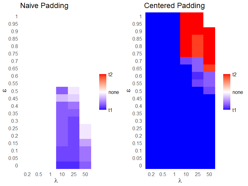
Figure 6: We fix $k=40$ and use the seeded GMMF algorithm to match $A$ with $B$ using 5 seeds randomly selected from the overlapping nodes of $B^{(1)}$ and $B^{(2)}$ as described in Section III-A. We plot the recovering results over $\varepsilon$ (here $\varepsilon$ is used to penalize the stronger of the two embedded templates) and $\lambda$, averaged by 20 Monte-Carlo simulations, where lighter means the recovered template is closer to $B^{(1)}$ (the stronger embedded template) and darker means the recovered template is closer to $B^{(2)}$ (the weaker embedded template). Note that the naive padding never recovered anything closer to $B^{(2)}$.

We fix $k=10$ (see Appendix V-B1 for the case of $k=15,40$), and use the seeded GMMF algorithm with 5 seeds randomly selected from the overlapping nodes of $B^{(1)}$ and $B^{(2)}$. In Figure 1 we use the naive padding (left) and the centered padding (right) and plot results over numerous choices of $\varepsilon$ (here $\varepsilon$ is used to penalize the stronger of the two embedded templates) and $\lambda$, averaged over 20 Monte-Carlo simulations. In the figures, stronger colors represent better recovery of the embedded templates, and t1 (blue) stands for template 1, t2 (red) stands for template 2, with white squares corresponding to the case when none of the two templates was recovered. From the figures, we see that when $\varepsilon$ is small we recover the stronger embedded template $(B_{1})$, and as $\varepsilon$ increases we move away from the stronger embedded template, and—provided a suitable value of $\lambda$—we successfully recover the weaker embedded template as desired. From the plots, we can see the centered padding outperforms the naive padding for recovering the second template in this multiple correlated Erdős-Rényi model, which aligns with the results proven in [31]. The phenomenon is clearer for larger $k$ (see, for example, Figure 6 in the Appendix), where the naive padding detects either only template 1 or nothing (denoted by the white in the plot) for whatever $\lambda$ we choose.

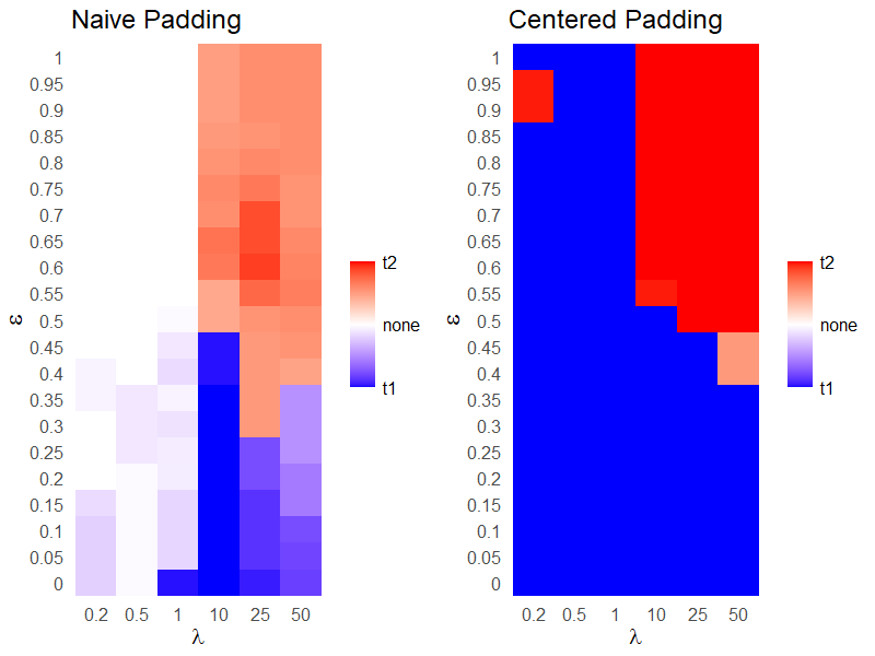
Figure 1: We fix $k=10$ and use the seeded GMMF algorithm to match $A$ with $B$ using 5 seeds randomly selected from the overlapping nodes of $B^{(1)}$ and $B^{(2)}$ as described in Section III-A. We plot the recovering results over $\varepsilon$ (here $\varepsilon$ is used to penalize the stronger of the two embedded templates) and $\lambda$, averaged by 20 Monte-Carlo simulations. In the figures, stronger colors represent better recovery of the embedded templates, and t1 (blue) stands for template 1, t2 (red) stands for template 2, with white squares corresponding to the case when none of the two templates was recovered.

Figure 2: We fix $k=10,\lambda=25$ and use the seeded GMMF algorithm with the centered padding to match $A$ with $B$ using 5 seeds randomly selected from the overlapping nodes of $B^{(1)},B^{(2)}$ and $B^{(3)}$, where $B^{(1)},B^{(2)}$ and $B^{(3)}$ are induced subgraph of $B$ such that graphs $A$ and $B$ follows multiple correlated ER model as described in Section III-B. We plot the recovering results over $\varepsilon_{1}$ (penalty applied to the diagonal elements of $S^{(11)},S^{(22)}$) and $\varepsilon_{2}$ (penalty applied to the diagonal elements of $S^{(13)},S^{(22)}$), averaged by 20 Monte-Carlo simulations. In the figure, the different patterns represent which template was recovered (in majority): t1 for template 1, t2 for template 2, and t3 for template 3, with white squares corresponding to the case when none of the three templates was recovered.

III-B Three overlapping templates

To better illustrate the iterative feature of the proposed algorithm, we construct a multiple correlated Erdős-Rényi model with $N=3$ and apply our algorithm to attempt to recover all of the three embedded templates. In this experiment, we take $\Lambda^{(1)}=0.8^{50\times 50},\Lambda^{(2)}=0.8^{500\times 500}$,

$$R_{1}=\bordermatrix{&m-k&k\cr m-k&R_{1}^{11}&R_{1}^{12}\cr k&(R_{1}^{12})^{T}&R_{1}^{22}};$$

$$R_{2}=\bordermatrix{&k&m-k\cr k&R_{1}^{22}&R_{2}^{12}\cr m-k&(R_{2}^{12})^{T}&R_{2}^{22}}$$

and

$$R_{3}=\bordermatrix{&k&m-k\cr k&R_{1}^{22}&R_{3}^{12}\cr m-k&(R_{3}^{12})^{T}&R_{3}^{22}},$$

where $R_{1}^{11}$ and $R_{1}^{12}$ are matrices with all entries set to 0.954; $R_{2}^{12}$ and $R_{2}^{22}$ are matrices with all entries set to $0.803$; $R_{3}^{12}$ and $R_{3}^{22}$ are matrices with all entries set to $0.706$; and $R^{22}_{1}$ is a matrix with all entries set to 0.897. Note again this structure ensures the induced subgraphs $B^{(1)},B^{(2)}$ and $B^{(3)}$ have exactly $k$ pairwise overlapping nodes, and to make the $B^{(1)}$ a better probabilistic match (i.e., a stronger embedding) than $B^{(2)}$ which is a better probabilistic match than $B^{(3)}$.

For the similarity matrix $S$, we set $S$ to be

$$\bordermatrix{&m-k&k&m-k&m-k&n-3m+2k\cr m-k&S^{(11)}&S^{(12)}&S^{(13)}&S^{(14)}&S^{(15)}\cr k&S^{(21)}&S^{(22)}&S^{(23)}&S^{(24)}&S^{(25)}}$$

where all entries of $S$ are independent Beta random variables, such that

$$\text{ the diagonal elements of }S^{(11)}\sim\operatorname{Beta}(\mu=0.7)$$

$$\text{ the diagonal elements of }S^{(22)}\sim\operatorname{Beta}(\mu=0.6)$$

$$\text{ the diagonal elements of }S^{(13)}\sim\operatorname{Beta}(\mu=0.55)$$

$$\text{ the diagonal elements of }S^{(14)}\sim\operatorname{Beta}(\mu=0.5)$$

and all other entries are sampled from $\operatorname{Beta}(\mu=0.1)$. Again for all the Beta distributions, we randomly sample $\alpha\sim U(0,1)$ and use the specified $\mu$ to calculate the corresponding $\beta$.

In Figure 2, we fix $k=10,\lambda=25$ (see Appendix V-B2 for other combinations of $(k,\lambda)$), and use the seeded GMMF algorithm with the centered padding (the naive padding behaved sub-optimally for recovering template 3, see Appendix V-B2 for details) and 5 seeds randomly selected from the overlapping nodes of $B^{(1)},B^{(2)}$ and $B^{(3)}$. We plot the recovering results over $\varepsilon_{1}$ (penalty applied to the diagonal elements of $S^{(11)},S^{(22)}$) and $\varepsilon_{2}$ (penalty applied to the diagonal elements of $S^{(13)},S^{(22)}$), averaged by 20 Monte-Carlo simulations. In the figure, the different patterns represent which template was recovered (in majority): t1 for template 1, t2 for template 2, and t3 for template 3, with white squares corresponding to the case when none of the three templates was recovered. As we can see, when both $\varepsilon_{1},\varepsilon_{2}$ are small, we recover the strongest embedded template; as $\varepsilon_{1}$ increases, we move away from the strongest embedded template to the second strongest embedded template; finally when both $\varepsilon_{1},\varepsilon_{2}$ get large enough, we recovered the third embedded template as desired.

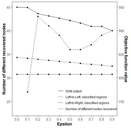
Figure 3: We run our proposed algorithm using the seeded GMMF algorithm with 500 restarts and 5 seeds selected from the node pairs $\{(s_{j},w_{j})\}_{j=1}^{6}$ as described in III-C, taking the result with highest objective function value (Eq. 2) as the output. For each $\varepsilon$, we compute the GM objective function value (left axis) of the resulting matrix with the template; we also computed the objective function value with respect to the alignment given by the template to the same classified brain region in the left hemisphere in $B$ (Left–to–Left in the plot), as well as the objective function value given by the template to the symmetric region from the right hemisphere in $B$ (Left–to–right in the plot). Also for $\varepsilon>0$, we calculated the number of novel nodes recovered in each matching compared to the subgraph detected with $\varepsilon=0$ (right axis).

III-C MRI Brain data

We now apply the proposed algorithm to a real data set of human connectomes from [40], where we consider the BNU1 test-retest connectomes processed via the pipeline at [15] (see http://fcon_1000.projects.nitrc.org/indi/CoRR/html/bnu_1.html and https://neurodata.io/mri/ for more detail). The dataset consist of test-retest DTI data for each patient processed into connectome graphs. Moreover, the brain graphs here are segmented into regions of interest and contain $(x,y,z)$ DTI coordinates. We chose patient “subj1” for our present experiment. In the first connectome, which contains 1128 nodes, we select a region (region 30) with 46 nodes from the left hemisphere to act as our template. We then extracted the subgraph induced by the selected region and considered it as our graph $A$. The entire graph of the other brain scan from the same patient, which contains 1129 nodes, was designated as our graph $B.$ Our goal is to recover both the same region of interest in the left hemisphere (we consider this the “strong” embedded template) and the corresponding region (region 65) in the right hemisphere (the “weak” embedded template).

To construct the similarity matrix, we consider the $(x,y,z)$ coordinates of each node in the processed MRI scan from graphs $A$ and $B$. Subsequently, we randomly selected 12 nodes, denoted as $s=\{s_{1},\ldots,s_{12}\}$, from graph $A$. For nodes ${s_{1},\ldots,s_{6}}$, we identified the corresponding nodes ${w_{1},\ldots,w_{6}}$ from the same region, same hemisphere, in graph $B$. Whereas for nodes ${s_{7},\ldots,s_{12}}$, we identified the corresponding nodes ${w_{7},\ldots,w_{12}}$ from the corresponding region in the other hemisphere relative in graph $B$. Note, these are not seeded vertices, but are simply used to construct the similarity matrix $S$. Informally, we consider each pair of $(s_{i},w_{i})$ as a “bridge” which has distance 0; allowing us to define a suitable distance across hemispheres for any nodes $u\in A$ and $v\in B$ as follows. Setting the distance between corresponding seeded nodes across hemispheres to be $0$, we define the distance via

$$d(u,v)=\min_{j\in[12]}\{\|u-s_{i}\|_{2}+\|v-w_{i}\|_{2}\}$$

Here, $\|\cdot\|_{2}$ represents the standard Euclidean distance. We defined our similarity matrix such that $S_{ij}\propto-d(u_{i},v_{j})$.

We executed our proposed algorithm using the seeded GMMF algorithm with 500 restarts, with 5 seeds selected out of the node pairs $\{(s_{j},w_{j})\}_{j=1}^{6}$, so the seeds exist in the left-hemisphere only; and we selected the result with the highest objective function value (in Eq. 2 using naive padding with $\lambda=0.1$ as the final match; see appendix V-B3 for the case of $\lambda=1$). Naive padding worked well with the irregular structure of the brain networks here, and we are actively researching whether centered or naive padding is more appropriate in non edge-independent models. For each $\varepsilon$, (plotted in Figure 3) we compute the GM objective function value (right axis) of the resulting matrix with the template; we also computed the objective function value with respect to the alignment given by the template to the same classified brain region in the left hemisphere in $B$ (Left–to–Left in the plot), as well as the objective function value given by the template to the symmetric region from the right hemisphere in $B$ (Left–to–Right in the plot). Also for $\varepsilon>0$, we calculated the number of novel nodes recovered in each matching compared to the subgraph detected with $\varepsilon=0$ (left axis, “Number of different nodes recovered” in the plot). As expected, the objective function value obtained from the output of the seeded GMMF algorithm is better than the ground truth alignment. Furthermore, by increasing $\varepsilon$ beyond 0.1, we observed a deviation from the original recovered template, leading to the discovery of a new subgraph matching the template close to optimally. We comment that the decrease in the objective function value based on the alignment provided by the classified brain regions across the scans is a result of the seeds in the SGM algorithm, where the similarity scores between these 5 seeds pairs decrease as $\varepsilon$ increases.

III-D Template discovery in TKBs

For our second real data example, we consider the transactional knowledge base (TKB) of [26]. The graph is constructed from a variety of information sources including news articles, Reddit, Venmo, and bibliographic data. Moreover, nodes and edges are richly attributed. Node attributes include a unique node ID, node type (according to a custom ontology), free text value, entry ID (used to identify the node in the Wikidata Knowledge Base), date and latitude/longitude. Edge attributes include a unique edge ID, edge type (according to a custom ontology), and edge argument (providing additional edge information). See [26] for more information on the construction of this network and details on the custom ontological structure.

Along with the large background graph, [26] describes the creation of multiple signal templates to search for in the background, each with varying levels of noise. In addition to perfectly aligned templates (i.e., subgraphs of the background isomorphic to the template), templates are embedded with different and varying noise levels, necessitating noisy template recovery.

The full graph has 14,220,800 nodes and 157,823,262 edges. For each template, we do some simple preprocessing of the graphs that reduces their size (for instance, removing node types that do not appear in the template, removing dangling edges, etc). This preprocessing yields the pruned graphs that are fed into our matching algorithm, which have approximately $13\times 10^{6}$ nodes and $32\times 10^{6}$ edges. As in [24], we create a multiplex network from this TKB by dividing edge types (from the different sources) and different ontological edge types into multiple weighted graph layers (weighted based on a measure of ontological similarity), and using node features to define a node–to–node similarity matrix. Note that we use naive padding here, as the edge structure is naturally weighted and optimal centering in the weighted case is nuanced and the subject of present study. The multiplex adaptation of the GMMF procedure can be found in [24], and amounts to adapting the Frank-Wolfe approach to the objective functions (recall $P=\bordermatrix{&n\cr m&P_{(1)}\cr n-m&P_{(2)}}$):

$$\underset{P\in\Pi_{n}}{\text{argmax}}\operatorname{trace}\Big{(}\Big{[}A^{(i)}\oplus 0_{n-m,n-m}\Big{]}PB^{(i)}P^{T}\Big{)}$$

$$+ \lambda\operatorname{trace}\left(SP_{(1)}\right)$$

where $A^{(i)}$ (resp., $B^{(i)}$) represent the template structure (resp., background structure) in layer $i$ of the multiplex graph and where nodes with a common label across layers are assumed aligned.

We show the effect of the solution diversification via the following experiment. To measure the fidelity of recovered templates when no ground truth is present, we use the graph edit distance (GED) metric outlined in [10]. We run 32 random restarts of the GMMF algorithm for each template recovery (we plot results for template 1A, 1B, 1C, 1D here; results for templates 2 and 3 can be found in Appendix V-B4), plotting the empirical CDF of the GED of the recovered templates; results are plotted in Figure 4. Different penalization values are represented with different colors in the plot.

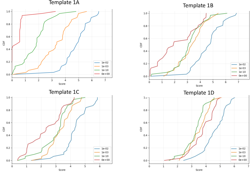
Figure 4: We run 32 random restarts of the GMMF algorithm for each template recovery, plotting the empirical CDF of the GED of the recovered templates. Different penalization values are represented with different colors in the plot.

Note that in each template, version A has an isomorphic copy in the background while this is not guaranteed for the other templates (as they have noise introduced in the embeddings). From Figure 4, we see that the solution diversification is successful at yielding recovered templates including our optimal fits (the best recovered templates in the $\epsilon=0$ case) and templates that are close to optimal by GED. These templates further recover significant signal not recovered in the $\epsilon=0$ case; see Table I. In the table, for each vertex in the template we show how many vertices in the background have similarity greater than 0 (i.e., are potential matches)—this is shown in the #$>0$ row. We see that the solution diversification is successful at recovering additional possible matches in the suboptimal recovered templates. We also see that too severe of a penalty (here the $\epsilon=0.01$ case) yields fewer unique nodes and worse GED fits. While choosing an optimal $\epsilon$ is of paramount importance, we do not have a fully principled recommendation for a best choice. We do recommend smaller penalty combined with more random restarts which achieved our best results.

node	1	2	3	4	5	6	7	8	9	10	11	12	13	14	15
$\epsilon=0$	1	8	1	3	20	1	1	1	3	1	14	2	1	1	5
$\epsilon=0.01$	1	23	2	15	32	1	1	1	8	1	24	5	4	1	24
$\epsilon=10^{-3}$	4	21	20	29	32	5	5	4	27	1	26	5	27	3	31
$\epsilon=10^{-10}$	4	32	30	32	31	5	5	4	32	5	30	5	32	4	32
#$>0$	4	32	32	32	32	5	5	4	32	5	32	5	32	4	32
node	16	17	18	19	20	21	22	23	24	25	26	27	28	29	30
$\epsilon=0$	1	1	1	1	2	3	1	3	19	1	1	1	3	4	1
$\epsilon=0.01$	1	1	1	1	3	16	1	14	32	1	2	2	5	18	1
$\epsilon=10^{-3}$	1	4	4	3	3	27	5	26	31	12	5	4	5	27	4
$\epsilon=10^{-10}$	4	20	4	3	3	32	5	32	32	29	5	4	5	32	4
#$>0$	4	32	4	3	3	32	5	32	32	32	5	4	5	32	4
node	31	32	33	34	35	36	37
$\epsilon=0$	3	4	1	2	4	1	1
$\epsilon=0.01$	3	25	1	2	5	1	1
$\epsilon=10^{-3}$	13	31	4	15	5	5	6
$\epsilon=10^{-10}$	28	32	4	31	5	5	21
#$>0$	32	32	4	32	5	5	32

TABLE I: In Template 1A, we list for each node how many vertices in the background have similarity greater than 0 (i.e., are potential matches)—this is shown in the #$>0$ row). We then show for the different penalization levels, how many of these possible matches were recovered across the 32 random restarts.

IV Conclusion and discussion

In this paper, we have introduced a workflow for iteratively identifying multiple instances of noisy embedded templates within a large graph. Our approach extends the matched-filters-based method for noisy subgraph detection by considering both the edgewise structure and node feature similarities. By incorporating these factors, we have achieved a more diversified and scalable approach to effectively uncover embeddings of noisy copies of graph templates. The theoretical analysis of our algorithm demonstrates that, under the assumption of a strong correlation between the edgewise structural similarities and node-wise feature similarities, our approach can successfully identify multiple embedded templates within a large network. To validate the effectiveness of our proposed workflow, we conducted experiments using simulations based on Multiple Erdős Rényi models, as well as real-world data sets such as human brain connectomes and the TKB dataset.

Furthermore, we present several intriguing questions that merit further exploration. In particular, the manuscript assumes an agreement between edge-structural similarity and node feature similarity. It would be valuable to investigate scenarios where such an agreement is absent, specifically identifying sharp parameter thresholds that lead to edge-structure dominated recovery, node-feature dominated recovery, and mixed-effect recovery. In all three cases, it is crucial to establish robust measures for evaluating the correctness of edge-wise matching between the template and the recovered template. Additionally, we highlight the issue of overlapping nodes between two embedded templates. The reliability of our algorithm relies on the ratio of overlapping parts between the templates being moderate. However, if the ratio is excessively high, penalizing already recovered templates may lead to sub-optimal results. To address this concern, it would be beneficial to develop methods that specifically target penalization on the non-overlapping regions while preserving the signal of the overlapping region, thereby enhancing the algorithm’s performance.

V Appendix

Herein, we collect proofs of our main theoretical results as well as additional experiments.

V-A Proof of Theorem 2:

We restate Theorem 2 here before providing a proof.

Theorem 2: Let $A$ and $B$ be two graphs constructed as above. If there is a constant $\alpha\in[1/2,1)$ such that

• $m-k=\Theta(m)$; $m^{1-\alpha}=\omega(\log^{4}n)$

• $\lambda=m^{\alpha}$;

• $(r_{1}-r_{3})\ll m^{\alpha-1}$; $r_{1}>r_{2}>r_{3}$ are bounded away from $0$ and $1$;

• $\mu_{3}>(1-\varepsilon)\mu_{1}$ and $(1-\varepsilon)\mu_{2}>\mu_{4}$; the differences $\mu_{3}-(1-\varepsilon)\mu_{1}$, $(1-\varepsilon)\mu_{2}-\mu_{4}$, and $\mu_{3}-\mu_{4}$ are bounded away from 0;

• $p=p_{n}$ is bounded away from $0$ and $1$;

then if $\widetilde{\Pi}$ is the set of permutations perfectly aligning the weakly embedded template, we have that

$$\mathbb{P}(\text{argmax}_{P\in\Pi}f_{\varepsilon,\lambda}(P)\subset\widetilde{\Pi})\geq 1-e^{-\omega(\log n)}.$$

Proof.

Let $P^{*}$ be (any one of) the permutation that maps $A$ to the strongly embedded template in $B$, and $\widetilde{P}$ (any one of) the permutation that maps $A$ to the weakly embedded template in $B$. Finally, let $P$ be an arbitrary permutation in $\Pi_{n}$ that does not map $A$ to the weakly embedded template in $B$. We first calculate the expected value of the objective function, where $\sigma_{P}$ is the permutation described by the matrix $P$.

We first consider the contribution to the objective function of the edge disagreement induced by $P$. Let $C_{v}=p(1-p)$. Let $T_{1}$ be the set of nodes that $P$ correctly aligns within the strongly embedded template, and $T_{2}$ the set of nodes that $P$ matches correctly to the weakly embedded template. Now, we have

$$\mathbb{E}\left\{\operatorname{tr}\left(\widetilde{A}P\widetilde{B}P^{T}\right)\right\}= \mathbb{E}\left\{\sum_{i=1}^{m}\sum_{j=1}^{m}(2A_{ij}-1)(2B_{\sigma_{P}(j)\sigma_{P}(i)}-1)\right\}$$

$$= \sum_{i=1}^{m}\sum_{j=1}^{m}\mathbb{E}\left[4A_{ij}B_{\sigma_{P}(j)\sigma_{P}(i)}-2A_{ij}-2B_{\sigma_{P}(j)\sigma_{P}(i)}+1\right]$$

Thus,

$$\mathbb{E}\left\{\operatorname{tr}\left(\widetilde{A}P\widetilde{B}P^{T}\right)\right\}= 8\binom{m}{2}(p^{2}-p)+4\sum_{i=1}^{m}\sum_{j=1}^{m}r_{g_{ij}}C_{v}+m^{2}$$

where

$$g_{ij}=\begin{cases}1,&\text{if }\{i,j\}\in\binom{T_{1}}{2}\setminus\binom{T_{2}}{2};\\ 2,&\text{if }\{i,j\}\in\binom{T_{1}}{2}\cap\binom{T_{2}}{2};\\ 3,&\text{if }\{i,j\}\in\binom{T_{2}}{2}\setminus\binom{T_{1}}{2};\\ 0,&\text{otherwise}.\end{cases}$$

Let the counts of the correctly recovered template edges via $P$ and $\tilde{P}$ be denoted

	Recovers edges in $\binom{T_{1}}{2}\cap\binom{T_{2}}{2}$	Recovers edges in $\binom{T_{2}}{2}\setminus\binom{T_{1}}{2}$
Recovers edges in $\binom{T_{1}}{2}\setminus\binom{T_{2}}{2}$	$0$	$h_{1}$
Recovers edges in $\binom{T_{1}}{2}\cap\binom{T_{2}}{2}$	$j_{1}$	$0$
Recovers edges in $\binom{T_{2}}{2}\setminus\binom{T_{1}}{2}$	$0$	$h_{2}$
Misaligned template edges	$j_{2}$	$h_{3}$

Also, let $D_{E}(P):=\operatorname{tr}\left(\widetilde{A}\widetilde{P}\widetilde{B}\widetilde{P}^{T}\right)-\operatorname{tr}\left(\widetilde{A}P\widetilde{B}P^{T}\right)$, then

$$\mathbb{E}(D_{E}(P)) =\mathbb{E}\left\{\operatorname{tr}\left(\widetilde{A}\widetilde{P}\widetilde{B}\widetilde{P}^{T}\right)-\operatorname{tr}\left(\widetilde{A}P\widetilde{B}P^{T}\right)\right\}$$

$$=8C_{v}\left\{j_{2}r_{2}+h_{1}(r_{3}-r_{1})+h_{3}r_{3}\right\}$$

where we recall $C_{v}=p(1-p)$. We also know $j_{1}+j_{2}=k(k-1)/2,0\leq h_{1},h_{2}\leq\frac{m(m-1)}{2}-\frac{k(k-1)}{2}=\frac{(m-k)(m+k-1)}{2}$ and $\sum_{i=1}^{3}h_{i}=\frac{(m-k)(m+k-1)}{2}$.

We next consider the contribution to the objective function of the features/similarity induced by $P$. Now, we consider $S$ of the form

$$S=\bordermatrix{&m-k&k&m-k&n-2m+k\cr m-k&S^{(11)}&S^{(12)}&S^{(13)}&S^{(14)}\cr k&S^{(21)}&S^{(22)}&S^{(23)}&S^{(24)}}$$

where all entries of $S$ are independent—bounded in $[0,1]$—random variables, and where

$$\text{ the diagonal elements of }S^{(11)}\text{ have mean }\mu_{1}$$

$$\text{ the diagonal elements of }S^{(22)}\text{ have mean }\mu_{2}$$

$$\text{ the diagonal elements of }S^{(13)}\text{ have mean }\mu_{3}$$

and all other entries have mean $\mu_{4}$.

If the strongly embedded template is penalized, then $S$ is weighted via (where “$\circ$” is the matrix Hadamard product)

$${S^{(2,\epsilon)}}=\bordermatrix{&m-k&k&m-k&n-2m+k\cr m-k&(\mathbf{1}_{m-k,m-k}-\epsilon I_{m-k})\circ S^{(11)}&S^{(12)}&S^{(13)}&S^{(14)}\cr k&S^{(21)}&(\mathbf{1}_{k,k}-\epsilon I_{k})\circ S^{(22)}&S^{(23)}&S^{(24)}}$$

Now, we have

$$\mathbb{E}\left[\operatorname{tr}\left(S^{(2,\epsilon)}P^{T}\right)\right]= \mathbb{E}\left\{\sum_{i=1}^{m}(1-\varepsilon)^{\mathbbm{1}\{\sigma_{P}(i)=\sigma_{P^{*}}(i)\}}S_{i,\sigma_{P}(i)}\right\}$$

$$= \sum_{i=1}^{m}(1-\varepsilon)^{\mathbbm{1}\{\sigma_{P}(i)=\sigma_{P^{*}}(i)\}}\mathbb{E}(S_{i,\sigma_{P}(i)})$$

$$= \sum_{i=1}^{m}(1-\varepsilon)^{\mathbbm{1}\{\sigma_{P}(i)=\sigma_{P^{*}}(i)\}}\mu_{h_{i}}$$

where

$$h_{i}=\begin{cases}1,&\text{if }i\in T_{1}\setminus T_{2};\\ 2,&\text{if }i\in T_{1}\cap T_{2};\\ 3,&\text{if }i\in T_{2}\setminus T_{1};\\ 4,&\text{otherwise}.\end{cases}$$

Now, consider $D_{F}(P):=\operatorname{tr}\left(S^{(2,\epsilon)}\tilde{P}^{T}\right)-\operatorname{tr}\left(S^{(2,\epsilon)}P^{T}\right)$. Let the counts of the recovered template nodes via $P$ and $\tilde{P}$ be denoted

	Recovers $T_{1}\cap T_{2}$	Recovers $T_{2}\setminus T_{1}$
Recovers $T_{1}\setminus T_{2}$	$0$	$b_{1}$
Recovers $T_{1}\cap T_{2}$	$a_{1}$	$0$
Recovers $T_{2}\setminus T_{1}$	$0$	$b_{2}$
Misaligned template node	$a_{2}$	$b_{3}$

so that

$$\mathbb{E}(D_{F}(P)) =\mathbb{E}\left\{\operatorname{tr}\left(S^{(2,\epsilon)}\tilde{P}^{T}\right)-\operatorname{tr}\left(S^{(2,\epsilon)}P^{T}\right)\right\}$$

$$=a_{2}[(1-\varepsilon)\mu_{2}-\mu_{4}]+b_{1}[\mu_{3}-(1-\varepsilon)\mu_{1}]+b_{3}[\mu_{3}-\mu_{4}].$$

Note the following hold as well: $0\leq a_{1}\leq k,a_{1}+a_{2}=k,0\leq b_{1},b_{2}<m-k$ and $\sum_{i=1}^{3}b_{i}=m-k$. Also, note that

$$\binom{a_{1}}{2} =j_{1},\quad\binom{a_{2}}{2}+a_{1}a_{2}=j_{2},\quad\binom{b_{2}}{2}+b_{2}a_{1}=h_{2},$$

$$\binom{b_{1}}{2}+b_{1}a_{1} =h_{1},\quad\binom{b_{3}}{2}+b_{1}b_{2}+b_{1}b_{3}+b_{2}b_{3}+a_{2}(m-k)+b_{3}a_{1}=h_{3}.$$

We next note that if

$$P=\bordermatrix{&n&\cr m&P_{(1)}\cr n-m&P_{(2)}},\text{ and }P^{\prime}=\bordermatrix{&n&\cr m&P_{(1)}\cr n-m&P^{\prime}_{(2)}},$$

then $f(P)=f(P^{\prime})$ regardless of whether $P_{(2)}=P_{(2)}^{\prime}$ or not. Also, note that the number of $P$ with the first $m$ rows exactly equal to $P_{(1)}$ is bounded above by (where $H(\cdot)$ is the binomial entropy function)

$$\binom{k}{a_{1}}\binom{m-k}{b_{1}}\binom{m-k}{b_{2}}n^{a_{2}+b_{3}}\leq 2^{kH\left(\frac{a_{1}}{k}\right)+(m-k)H\left(\frac{b_{1}}{m-k}\right)+(m-k)H\left(\frac{b_{2}}{m-k}\right)}n^{a_{2}+b_{3}}.$$

Let $g(P,\tilde{P})=f(P)-f(\tilde{P})$ so that

$$\mathbb{E}g(P,\widetilde{P}) =\mathbb{E}(D_{E}(P)+\lambda D_{F}(P))$$

$$=8C_{v}\Big{\{}\left(\binom{a_{2}}{2}+a_{1}a_{2}\right)r_{2}+\left(\binom{b_{1}}{2}+b_{1}a_{1}\right)(r_{3}-r_{1})$$

$$\hskip 14.22636pt+\left(\binom{b_{3}}{2}+b_{1}b_{2}+b_{1}b_{3}+b_{2}b_{3}+a_{2}(m-k)+b_{3}a_{1}\right)r_{3}\Big{\}}$$

$$\hskip 14.22636pt+\lambda(a_{2}[(1-\varepsilon)\mu_{2}-\mu_{4}]+b_{1}[\mu_{3}-(1-\varepsilon)\mu_{1}]+b_{3}[\mu_{3}-\mu_{4}])$$

$$\geq 8C_{v}\Big{\{}\underbrace{\left(\binom{b_{1}+a_{2}+b_{3}}{2}+(b_{1}+a_{2}+b_{3})(b_{2}+a_{1})\right)}_{:=n_{E}}r_{3}-\left(\binom{b_{1}}{2}+b_{1}a_{1}\right)r_{1}\Big{\}}$$

$$\hskip 14.22636pt+\lambda(\underbrace{a_{2}+b_{1}+b_{3}}_{:=n_{F}})*\underbrace{\min([(1-\varepsilon)\mu_{2}-\mu_{4}],[\mu_{3}-(1-\varepsilon)\mu_{1}],[\mu_{3}-\mu_{4}])}_{:=c_{\varepsilon}}$$

$$=8C_{v}\left(n_{E}r_{3}-\left(\binom{b_{1}}{2}+b_{1}a_{1}\right)r_{1}\right)+\lambda n_{F}c_{\varepsilon}.$$

Considering the case where $b_{1}=m-k$ and $a_{1}=k$, we see that for the above expectation to be diverging to infinity, it suffices that

$$\lambda c_{\varepsilon}\gg(r_{1}-r_{3})(m{+}k)C_{v};$$ (3)

we will assume this holds for the remainder of the proof.

From the forms of $D_{E}(P)$ and $D_{F}(P)$, we have that $g(P,\widetilde{P})$ is a function of at most (as $P$ and $\widetilde{P}$ agree on $b_{2}+a_{1}$ template vertices and disagree on the rest)

$$\underbrace{2m-2b_{2}-2a_{1}}_{\text{from }D_{F}(P)}+\underbrace{\binom{m-b_{2}-a_{1}}{2}+(m-b_{2}-a_{1})(b_{2}+a_{1})}_{\text{from }D_{E}(P)}$$

random variables, and changing any of the variables from $D_{F}(P)$ can change $g(P,\widetilde{P})$ by at most $4\lambda$, and changing any of the variables from $D_{E}(P)$ can change $g(P,\widetilde{P})$ by at most a bounded constant (bounded above by 8 for example). Lastly, note that $m-b_{2}-a_{1}=b_{1}+b_{3}+a_{2}=n_{F}$ and

$$\binom{m-b_{2}-a_{1}}{2}+(m-b_{2}-a_{1})(b_{2}+a_{1})=\binom{b_{1}+a_{2}+b_{3}}{2}+(b_{1}+a_{2}+b_{3})(b_{2}+a_{1})=n_{E}.$$

Note that

$$n_{E}=n_{F}\left(\frac{n_{F}-1}{2}+b_{2}+a_{1}\right)$$

Assume that $\varepsilon$ is such that $(1-\varepsilon)\mu_{2}>\mu_{4}$ and $(1-\varepsilon)\mu_{1}<\mu_{3}$, and that the differences

$$(1-\varepsilon)\mu_{2}-\mu_{4},\quad\mu_{3}-\mu_{4},\text{ and }\mu_{3}-(1-\varepsilon)\mu_{1}$$

are bounded away from $0$. Note that if Eq. (3) holds, then

$$\lambda n_{F}c_{\varepsilon} \gg n_{F}(r_{1}-r_{3})(m+k)C_{v}$$

$$\gtrsim\binom{b_{1}}{2}(r_{1}-r_{3})C_{v}$$

$$\gtrsim C_{v}\left(\left(\binom{b_{1}}{2}+b_{1}a_{1}\right)r_{1}-r_{3}n_{E}\right)$$

and $\mathbb{E}g(P,\widetilde{P})=\Omega(\lambda n_{F}c_{\varepsilon})$. An application of McDiarmid’s inequality then yields that for $n$—and hence $m=m_{n}$—sufficiently large, (where $\xi>0$ is a constant that can change line–to–line)

$$\mathbb{P} (|g(P,\widetilde{P})|\geq 0)\leq\mathbb{P}(|g(P,\widetilde{P})-\mathbb{E}[g(P,\widetilde{P})]|\geq\mathbb{E}[g(P,\widetilde{P})])$$

$$\leq 2\exp\left\{-\xi\frac{C_{v}^{2}\left(n_{E}r_{3}-\left(\binom{b_{1}}{2}+b_{1}a_{1}\right)r_{1}\right)^{2}+\lambda^{2}n_{F}^{2}c_{\varepsilon}^{2}}{n_{E}+\lambda^{2}n_{F}}\right\}$$

$$\leq 2\exp\left\{\!-\xi\frac{C_{v}^{2}\!\left(\left(b_{3}^{2}+a_{2}^{2}\!+\!(b_{1}\!+\!b_{3}\!+\!a_{2})(b_{2}+a_{1})\right)r_{3}\!-\!b_{1}^{2}(r_{1}\!-\!r_{3})\right)^{2}\!+\!m^{2\alpha}n_{F}^{2}c_{\varepsilon}^{2}}{m^{2\alpha}n_{F}}\right\}$$ (4)

Recall that $\lambda=m^{\alpha}$, so that Eq. (3) requires $(r_{1}-r_{3})=o(m^{\alpha-1})$. A union bound over all $P$ with the same counts ($a$’s and $b$’s) as $P$, modulo the equivalence between permutations with the same first $m$ rows, and a union bound over all possible counts of the $a$’s and $b$’s then yields (where $\xi>0$ is a constant that can change line–to–line)

$$\mathbb{P}(\exists\,P\neq\widetilde{P}\text{ s.t. }|g(P,\widetilde{P})|\geq 0)\leq$$

$$\sum_{a_{1}=0}^{k}\sum_{b_{1}=0}^{m-k}\sum_{b_{2}=0}^{m-k-b_{1}}2\exp\Bigg{\{}\!-\xi\frac{C_{v}^{2}\!\left(\left(b_{3}^{2}+a_{2}^{2}\!+\!(b_{1}\!+\!b_{3}\!+\!a_{2})(b_{2}+a_{1})\right)r_{3}\!-\!b_{1}^{2}(r_{1}\!-\!r_{3})\right)^{2}\!+\!m^{2\alpha}n_{F}^{2}c_{\varepsilon}^{2}}{m^{2\alpha}n_{F}}$$

$$\hskip 28.45274pt+kH\left(\frac{a_{1}}{k}\right)\log(2)+(m-k)H\left(\frac{b_{1}}{m-k}\right)\log(2)+(m-k)H\left(\frac{b_{2}}{m-k}\right)\log(2)$$

$$\hskip 28.45274pt+(a_{2}+b_{3})\log(n)\Bigg{\}}$$ (5)

To tackle the above Eq. (5), we consider several cases:

• If $b_{3}^{2}=\Omega(m^{3/2+\alpha/2})$ or $a_{2}^{2}=\Omega(m^{3/2+\alpha/2})$, then the exponential in Eq. (5) can be bounded above by (where $\xi>0$ is a constant that can change line–to–line)

  $$2\exp\left\{-\xi\frac{C_{v}^{2}m^{3+\alpha}}{m^{2\alpha}n_{F}}+m\log n\right\}\leq 2\exp\Big{\{}-\xi C_{v}^{2}m(\underbrace{m^{2-\alpha}-\log n}_{:=\Theta(m^{2-\alpha})})\Big{\}}=e^{-\omega(\log n)}$$ (6)

• We next consider the case where both $b_{3}^{2}=o(m^{3/2+\alpha/2})$ and $a_{2}^{2}=o(m^{3/2+\alpha/2})$, in this case either $b_{1}=\Theta(m)$, $b_{2}=\Theta(m)$, or both are $\Theta(m)$.

  • $b_{1}=\Theta(m)$ and $b_{2}=\Theta(m)$: Then the $b_{1}*b_{2}$ term in the exponent in Eq. (5) yields the upper bound (where $\xi>0$ is a constant that can change line–to–line)

    $$2\exp\left\{-\xi\frac{C_{v}^{2}m^{4}}{m^{2\alpha}n_{F}}+m\log n\right\}\leq 2\exp\Big{\{}-\xi C_{v}^{2}m(\underbrace{m^{3-2\alpha}-\log n}_{:=\Theta(m^{3-2\alpha})})\Big{\}}=e^{-\omega(\log n)}$$ (7)

  • $b_{2}=o(m)$: In this case, $b_{1}(1+o(1))=m-k$. Note that if $x(1+o(1))=y$, then $x/y(1+o(1))=1$. If $x\leq y$, then $1-x/y=o(1)$. As $\lim_{z\rightarrow 0}-z\log_{2}z=0$, we then have

    $$yH(x/y) =y\left[\frac{x}{y}\underbrace{\left[-\log_{2}\left(\frac{x}{y}\right)\right]}_{=o(1)}+\underbrace{\left[-\left(1-\frac{x}{y}\right)\log_{2}\left(1-\frac{x}{y}\right)\right]}_{=o(1)}\right]$$

    $$=o(y)$$

    Similarly, if $y=\omega(1)$ and $x=o(y)$, then

    $$yH(x/y) =y\Bigg{[}\underbrace{-\frac{x}{y}\log_{2}\left(\frac{x}{y}\right)}_{=o(1)}+\left(1-\frac{x}{y}\right)\underbrace{\left[-\log_{2}\left(1-\frac{x}{y}\right)\right]}_{=o(1)}\Bigg{]}$$

    $$=o(y)$$

    The $n_{F}^{2}*m^{2\alpha}$ term in the exponent in Eq. (5) yields the upper bound (where $\xi>0$ is a constant that can change line–to–line; note by assumption $c_{\varepsilon}$ is bounded away from $0$)

    $$2\exp\Big{\{}-\xi\frac{n_{F}^{2}*m^{2\alpha}c_{\varepsilon}^{2}}{m^{2\alpha}n_{F}}+kH\left(\frac{a_{1}}{k}\right)\log(2)+(m-k)H\left(\frac{b_{1}}{m-k}\right)\log(2)$$

    $$\hskip 28.45274pt+(m-k)H\left(\frac{b_{2}}{m-k}\right)\log(2)+(a_{2}+b_{3})\log(n)\Bigg{\}}$$

    $$\leq 2\exp\Big{\{}-\xi mc_{\varepsilon}^{2}+o(m)+o(m^{3/4+\alpha/4}\log(n))\Bigg{\}}=2e^{-\omega(\log n)}$$ (8)

  • $b_{1}=o(m)$: In this case, $b_{2}(1+o(1))=(m-k)$. We make use here of the alternate bound where if $y=\omega(1)$ and $x=o(y)$, then (as $\lim_{z\rightarrow 0}-\log_{2}(1-z)/z=1/\log(2)$)

    $$yH(x/y) =y\Bigg{[}-\frac{x}{y}\log_{2}\left(\frac{x}{y}\right)-\left(1-\frac{x}{y}\right)\log_{2}\left(1-\frac{x}{y}\right)\Bigg{]}$$

    $$=O(x\log_{2}(y))+O\left(y\frac{x}{y}\left(1-\frac{x}{y}\right)\right)=O(x\log(y)).$$

    We also note that here

    $$( m-k)H\left(\frac{b_{2}}{m-k}\right)$$

    $$=(m-k)H\left(1-\frac{b_{1}+b_{3}}{m-k}\right)$$

    $$=(m-k)\left[-\left(1-\frac{b_{1}+b_{3}}{m-k}\right)\log_{2}\left(1-\frac{b_{1}+b_{3}}{m-k}\right)-\left(\frac{b_{1}+b_{3}}{m-k}\right)\log_{2}\left(\frac{b_{1}+b_{3}}{m-k}\right)\right]$$

    $$=O\left((m-k)\frac{b_{1}+b_{3}}{m-k}\left(1-\frac{b_{1}+b_{3}}{m-k}\right)\right)+O((b_{1}+b_{3})\log_{2}(m-k))$$

    $$=O((b_{1}+b_{3})\log(m-k))$$

    The $n_{F}^{2}*b_{2}^{2}$ term in the exponent in Eq. (5) yields the upper bound (where $\xi>0$ is a constant that can change line–to–line, and we use $kH\left(\frac{a_{1}}{k}\right)=kH\left(1-\frac{a_{2}}{k}\right)$ as above)

    $$2\exp\Big{\{}-\xi n_{F}m^{2-2\alpha}+kH\left(\frac{a_{1}}{k}\right)\log(2)+(m-k)H\left(\frac{b_{1}}{m-k}\right)\log(2)$$

    $$\hskip 28.45274pt+(m-k)H\left(\frac{b_{2}}{m-k}\right)\log(2)+(a_{2}+b_{3})\log(n)\Bigg{\}}$$

    $$\leq 2\exp\Big{\{}-\xi n_{F}m^{2-2\alpha}+O((b_{1}+b_{3}+a_{2})\log(m))+n_{F}\log(n)\Bigg{\}}=2e^{-\omega(\log n)}$$ (9)

Therefore, we have that Eq. (5) is bound above by

$$\mathbb{P}(\exists\,P\neq\widetilde{P}\text{ s.t. }|g(P,\widetilde{P})|\geq 0)\leq 2e^{-\omega(\log n)+\log k+2\log m}=2e^{-\omega(\log n)}$$

as desired. ∎

V-B More Experiments

V-B1 Additional two overlapping templates experiments

We first plot the cases of $k=15,k=40$ using the seeded GMMF algorithm with 5 seeds randomly selected from the overlapping nodes of $B^{(1)}$ and $B^{(2)}$, for the same parameters as described in III-A.

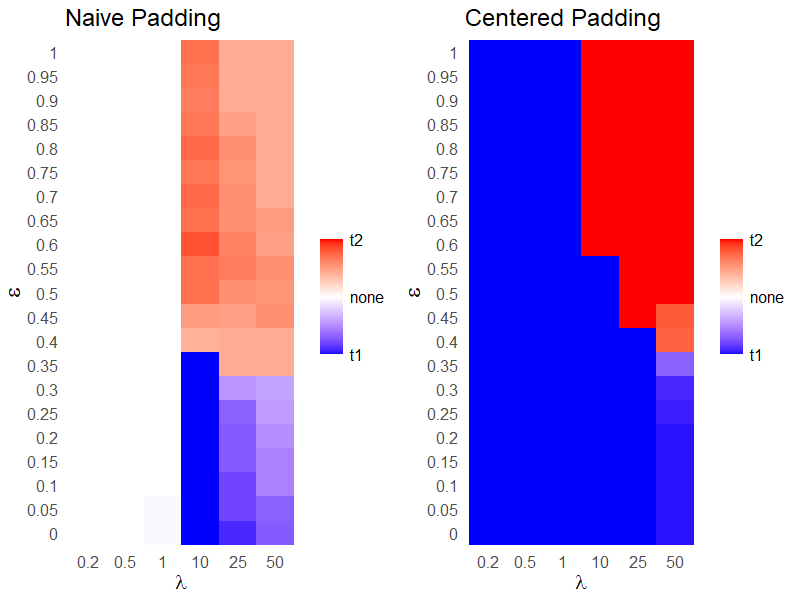
Figure 5: We fix $k=15$ and use the seeded GMMF algorithm to match $A$ with $B$ using 5 seeds randomly selected from the overlapping nodes of $B^{(1)}$ and $B^{(2)}$ as described in Section III-A. We plot the recovering results over $\varepsilon$ (here $\varepsilon$ is used to penalize the stronger of the two embedded templates) and $\lambda$, averaged by 20 Monte-Carlo simulations, where lighter means the recovered template is closer to $B^{(1)}$ (the stronger embedded template) and darker means the recovered template is closer to $B^{(2)}$ (the weaker embedded template).

V-B2 Additional three overlapping templates experiments

We first plot the simulated results where the parameters correspond to Figure 2 of III-B but with the naive padding.

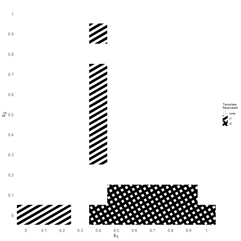
Figure 7: We fix $k=10,\lambda=25$ and use the seeded GMMF algorithm with the naive padding to match $A$ with $B$ using 5 seeds randomly selected from the overlapping nodes of $B^{(1)},B^{(2)}$ and $B^{(3)}$, where $B^{(1)},B^{(2)}$ and $B^{(3)}$ are induced subgraph of $B$ such that graphs $A$ and $B$ follows multiple correlated ER model as described in Section III-B. We plot the recovering results over $\varepsilon_{1}$ (penalty applied to the diagonal elements of $S^{(11)},S^{(22)}$) and $\varepsilon_{2}$ (penalty applied to the diagonal elements of $S^{(13)},S^{(22)}$), averaged by 20 Monte-Carlo simulations. In the figure, the different patterns represent which template was recovered (in majority): t1 for template 1, t2 for template 2, and we fail to recover template 3, with white squares corresponding to the case when none of the three templates was recovered.

Next, with the same correlation parameters $\{r_{j}\}_{j=1}^{4}$ and feature mean parameters $\{\mu_{j}\}_{j=1}^{5}$, we plot the simulated results for $k=10,\lambda=10$ and $k=40,\lambda=25$ using the centered padding.

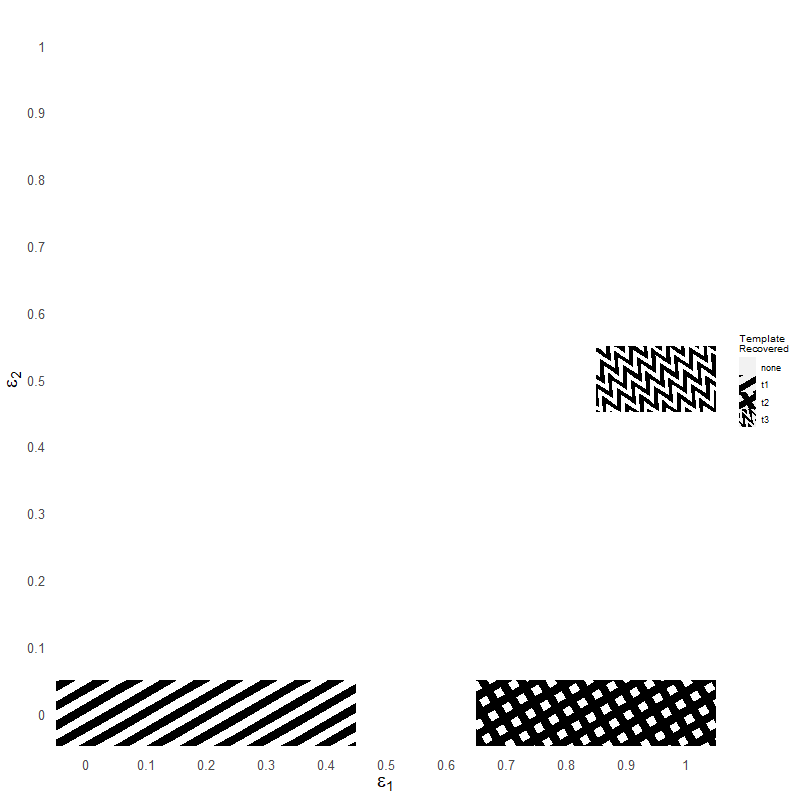
Figure 8: We fix $k=10,\lambda=10$ and use the seeded GMMF algorithm with the centered padding to match $A$ with $B$ using 5 seeds randomly selected from the overlapping nodes of $B^{(1)},B^{(2)}$ and $B^{(3)}$, where $B^{(1)},B^{(2)}$ and $B^{(3)}$ are induced subgraph of $B$ such that graphs $A$ and $B$ follows multiple correlated ER model as described in Section III-B. We plot the recovering results over $\varepsilon_{1}$ (penalty applied to the diagonal elements of $S^{(11)},S^{(22)}$) and $\varepsilon_{2}$ (penalty applied to the diagonal elements of $S^{(13)},S^{(22)}$), averaged by 20 Monte-Carlo simulations. In the figure, the different patterns represent which template was recovered (in majority): t1 for template 1, t2 for template 2, and t3 for template 3, with white squares corresponding to the case when none of the three templates was recovered.

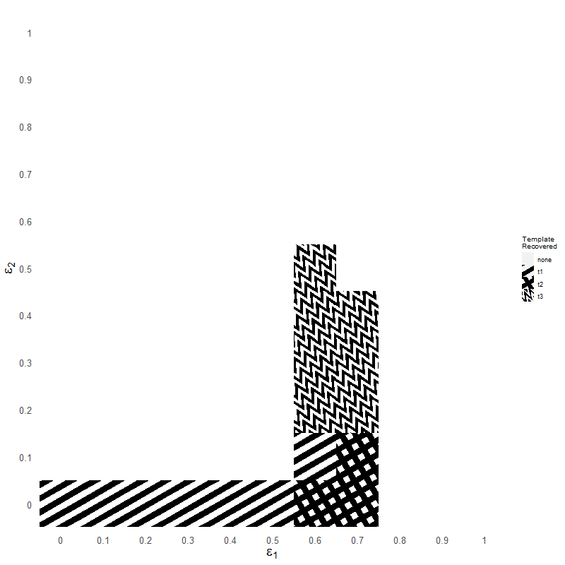
Figure 9: We fix $k=40,\lambda=25$ and use the seeded GMMF algorithm with the centered padding to match $A$ with $B$ using 5 seeds randomly selected from the overlapping nodes of $B^{(1)},B^{(2)}$ and $B^{(3)}$, where $B^{(1)},B^{(2)}$ and $B^{(3)}$ are induced subgraph of $B$ such that graphs $A$ and $B$ follows multiple correlated ER model as described in Section III-B. We plot the recovering results over $\varepsilon_{1}$ (penalty applied to the diagonal elements of $S^{(11)},S^{(22)}$) and $\varepsilon_{2}$ (penalty applied to the diagonal elements of $S^{(13)},S^{(22)}$), averaged by 20 Monte-Carlo simulations. In the figure, the different patterns represent which template was recovered (in majority): t1 for template 1, t2 for template 2, and t3 for template 3, with white squares corresponding to the case when none of the three templates was recovered.

V-B3 Additional Brain MRI plots

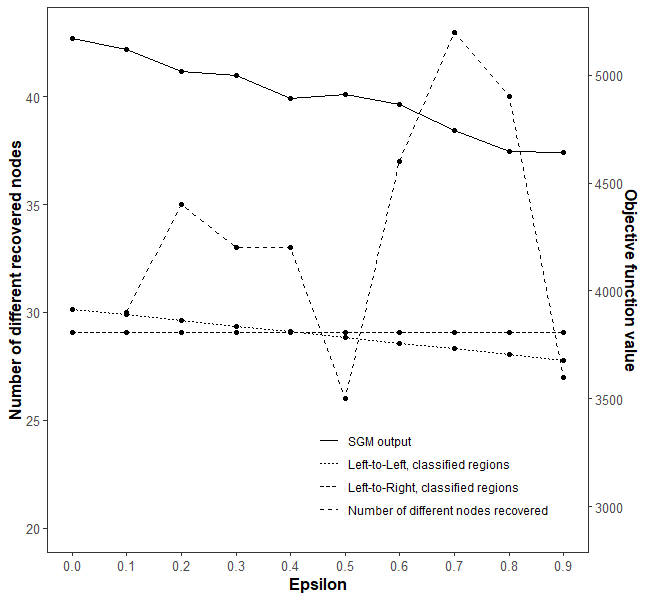
Figure 10: We run our proposed algorithm using the seeded GMMF algorithm with 500 restarts and 5 seeds selected from the node pairs $\{(s_{j},w_{j})\}_{j=1}^{6}$ as described in III-C, taking the result with highest objective function value (Eq. 2, $\lambda=1$) as the output. For each $\varepsilon$, we compute the GM objective function value (left axis) of the resulting matrix with the template; we also computed the objective function value with respect to the alignment given by the template to the same classified brain region in the left hemisphere in $B$ (Left–to–Left in the plot), as well as the objective function value given by the template to the symmetric region from the right hemisphere in $B$ (Left–to–right in the plot). Also for $\varepsilon>0$, we calculated the number of novel nodes recovered in each matching compared to the subgraph detected with $\varepsilon=0$ (right axis).

V-B4 Additional TKB templates

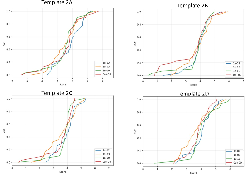
Figure 11: We run 32 random restarts of the GMMF algorithm for each template recovery, plotting the empirical CDF of the GED of the recovered templates. Different penalization values are represented with different colors in the plot.

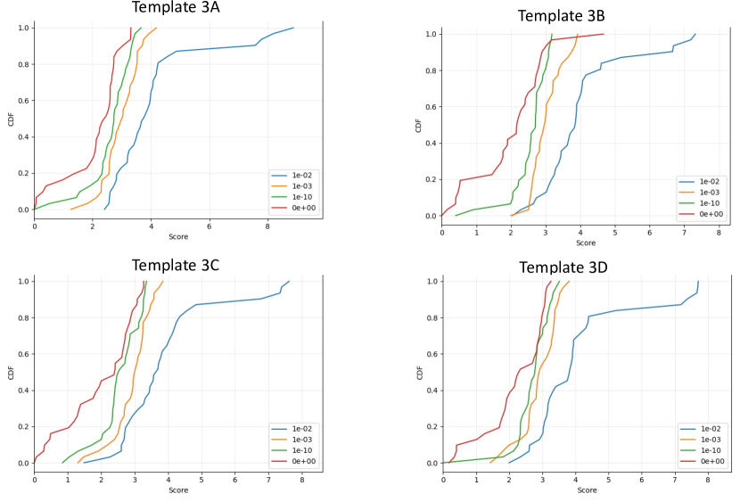
Figure 12: We run 32 random restarts of the GMMF algorithm for each template recovery, plotting the empirical CDF of the GED of the recovered templates. Different penalization values are represented with different colors in the plot.

References

- [1] M. A. Abdulrahim and M. Misra. A graph isomorphism algorithm for object recognition. Pattern Analysis and Applications, 1:189–201, 1998.
- [2] L. Babai. Graph isomorphism in quasipolynomial time. In Proceedings of the forty-eighth annual ACM symposium on Theory of Computing, pages 684–697, 2016.
- [3] S. Bhamidi, R. Van der Hofstad, and G. Hooghiemstra. First passage percolation on the Erdős–Rényi random graph. Combinatorics, Probability and Computing, 20(5):683–707, 2011.
- [4] J Bijsterbosch and A Volgenant. Solving the rectangular assignment problem and applications. Annals of Operations Research, 181:443–462, 2010.
- [5] B. Bollobás. Random graphs. Springer, 1998.
- [6] B. Bollobás, S. Janson, and O. Riordan. The phase transition in inhomogeneous random graphs. Random Structures and Algorithms, 31:3–122, 2007.
- [7] D. Conte, P. Foggia, C. Sansone, and M. Vento. Thirty years of graph matching in pattern recognition. International journal of pattern recognition and artificial intelligence, 18(03):265–298, 2004.
- [8] D. Cullina and N. Kiyavash. Improved achievability and converse bounds for erdos-renyi graph matching. In ACM SIGMETRICS Performance Evaluation Review, volume 44 (1), pages 63–72. ACM, 2016.
- [9] D. Cullina and N. Kiyavash. Exact alignment recovery for correlated erdos renyi graphs. arXiv preprint arXiv:1711.06783, 2017.
- [10] C. L. Ebsch, J. A. Cottam, N. C. Heller, R. D. Deshmukh, and G. Chin. Using graph edit distance for noisy subgraph matching of semantic property graphs. In 2020 IEEE international conference on big data (big data), pages 2520–2525. IEEE, 2020.
- [11] P. Erdős and A. Rényi. Asymmetric graphs. Acta Mathematica Academiae Scientiarum Hungarica, 14(3–4):295–315, 1963.
- [12] D.E. Fishkind, S. Adali, H.G. Patsolic, L. Meng, D. Singh, V. Lyzinski, and C.E. Priebe. Seeded graph matching. Pattern Recognition, 87:203 – 215, 2019.
- [13] M. Frank and P. Wolfe. An algorithm for quadratic programming. Naval Research Logistics Quarterly, 3(1-2):95–110, 1956.
- [14] A. Frieze and M. Karoński. Introduction to random graphs. Cambridge University Press, 2016.
- [15] G. Kiar, E. W. Bridgeford, W. R. G. Roncal, V. Chandrashekhar, D. Mhembere, S. Ryman, X. Zuo, D. S. Margulies, R. C. Craddock, C. E. Priebe, R. Jung, V. Calhoun, B. Caffo, R. Burns, M. P. Milham, and J. Vogelstein. A high-throughput pipeline identifies robust connectomes but troublesome variability. bioRxiv, page 188706, 2018.
- [16] H. W. Kuhn. The Hungarian method for the assignment problem. Naval Research Logistic Quarterly, 2:83–97, 1955.
- [17] V. Lyzinski. Information recovery in shuffled graphs via graph matching. IEEE Trans. on Information Theory, 64(5):3254–3273, 2018.
- [18] C. Mao, Y. Wu, J. Xu, and S. H. Yu. Random graph matching at otter’s threshold via counting chandeliers. arXiv preprint arXiv:2209.12313, 2022.
- [19] J. D. Moorman, Q. Chen, T. K. Tu, Z. M. Boyd, and A. L. Bertozzi. Filtering methods for subgraph matching on multiplex networks. In 2018 IEEE International Conf. on Big Data (Big Data), pages 3980–3985. IEEE, 2018.
- [20] J. D. Moorman, Q. Chen, T. K. Tu, Z. M. Boyd, and A. L. Bertozzi. Filtering methods for subgraph matching on multiplex networks. In 2018 IEEE International Conf. on Big Data (Big Data), pages 3980–3985, Dec 2018.
- [21] J. D. Moorman, T. Tu, Q. Chen, X. He, and A. Bertozzi. Subgraph matching on multiplex networks. IEEE Trans. on Network Science and Engineering, 2021.
- [22] E. Mossel and J. Xu. Seeded graph matching via large neighborhood statistics. Random Structures & Algorithms, 57(3):570–611, 2020.
- [23] D. R. Musser. Introspective sorting and selection algorithms. Software: Practice and Experience, 27(8):983–993, 1997.
- [24] K. Pantazis, D. L. Sussman, Y. Park, Z. Li, C. E. Priebe, and V. Lyzinski. Multiplex graph matching matched filters. Applied Network Science, 7(1):1–35, 2022.
- [25] J. D. Power, A. L. Cohen, S. M. Nelson, G. S. Wig, K. A. Barnes, J. A. Church, A. C. Vogel, T. O. Laumann, F. M. Miezin, B. L. Schlaggar, and S. E. Petersen. Functional network organization of the human brain. Neuron, 72(4):665–678, 2011.
- [26] S. Purohit, P. Mackey, W. Smith, M. Dunning, M. J. Orren, T. M. Langlie-Miletich, R. D. Deshmukh, A. Bohra, T. J. Martin, and D. J. Aimone. Transactional knowledge graph generation to model adversarial activities. In 2021 IEEE International Conference on Big Data (Big Data), pages 2662–2671. IEEE, 2021.
- [27] L. Ramshaw and R. E. Tarjan. On minimum-cost assignments in unbalanced bipartite graphs. HP Labs, Palo Alto, CA, USA, Tech. Rep. HPL-2012-40R1, 20, 2012.
- [28] K. Riesen, X. Jiang, and H. Bunke. Exact and inexact graph matching: Methodology and applications. Managing and mining graph data, pages 217–247, 2010.
- [29] C. Solnon. Experimental evaluation of subgraph isomorphism solvers. In Graph-Based Representations in Pattern Recognition: 12th IAPR-TC-15 International Workshop, GbRPR 2019, Tours, France, June 19–21, 2019, Proceedings 12, pages 1–13. Springer, 2019.
- [30] S. Sun and Q. Luo. In-memory subgraph matching: An in-depth study. In Proceedings of the 2020 ACM SIGMOD International Conference on Management of Data, pages 1083–1098, 2020.
- [31] D. L. Sussman, V. Lyzinski, Y. Park, and C. E. Priebe. Matched filters for noisy induced subgraph detection. IEEE Trans. on Pattern Analysis and Machine Intelligence, 42(11):2887–2900, 2019.
- [32] C. J. Thies, V. H. Metzler, T. M. Lehmann, and T. Aach. Formal extraction of biomedical objects by subgraph matching in attributed hierarchical region adjacency graphs. In Medical Imaging 2004: Image Processing, volume 5370, pages 1498–1508. SPIE, 2004.
- [33] T. K. Tu, J. D. Moorman, D. Yang, Q. Chen, and A. L. Bertozzi. Inexact attributed subgraph matching. In 2020 IEEE International Conf. on Big Data (Big Data), pages 2575–2582. IEEE, 2020.
- [34] Julian R Ullmann. An algorithm for subgraph isomorphism. Journal of the ACM (JACM), 23(1):31–42, 1976.
- [35] M. Wu, X. Li, C. Kwoh, and S. Ng. A core-attachment based method to detect protein complexes in ppi networks. BMC bioinformatics, 10(1):1–16, 2009.
- [36] Y. Wu, J. Xu, and S. H. Yu. Settling the sharp reconstruction thresholds of random graph matching. IEEE Transactions on Information Theory, 68(8):5391–5417, 2022.
- [37] J. Yan, X. Yin, W. Lin, C. Deng, H. Zha, and X. Yang. A short survey of recent advances in graph matching. In Proc. of the 2016 ACM on International Conf. on Multimedia Retrieval, pages 167–174. ACM, 2016.
- [38] D. Yang, Y. Ge, T. Nguyen, D. Molitor, J. D. Moorman, and A. L. Bertozzi. Structural equivalence in subgraph matching. IEEE Transactions on Network Science and Engineering, 2023.
- [39] S. Zhang, D. Zhou, M. Y. Yildirim, S. Alcorn, J. He, H. Davulcu, and H. Tong. Hidden: Hierarchical dense subgraph detection with application to financial fraud detection. In SDM, 2017.
- [40] X. Zuo, J. S. Anderson, P. Bellec, R. M. Birn, B. B. Biswal, J. Blautzik, J. Breitner, R. L. Buckner, V. D. Calhoun, F. X. Castellanos, et al. An open science resource for establishing reliability and reproducibility in functional connectomics. Scientific data, 1(1):1–13, 2014.