Density calculations of NGC 3783 warm absorbers using a time-dependent photoionization model

Outflowing wind as one type of AGN feedback, which involves noncollimated ionized winds prevalent in Seyfert-$1$ AGNs, impacts their host galaxy by carrying kinetic energy outwards. However, the distance of the outflowing wind is poorly constrained due to a lack of direct imaging observations, which limits our understanding of their kinetic power and therefore makes the impact on the local galactic environment unclear. One potential approach involves a determination of the density of the ionized plasma, making it possible to derive the distance using the ionization parameter $\xi$, which can be measured based on the ionization state. Here, by applying a new time-dependent photoionization model, tpho, in SPEX, we define a new approach, the tpho-delay method, to calculate/predict a detectable density range for warm absorbers of NGC $3783$. The tpho model solves self-consistently the time-dependent ionic concentrations, which enables us to study delayed states of the plasma in detail. We show that it is crucial to model the non-equilibrium effects accurately for the delayed phase, where the non-equilibrium and equilibrium models diverge significantly. Finally, we calculate the crossing time to consider the effect of the transverse motion of the outflow on the intrinsic luminosity variation. It is expected that future spectroscopic observations with more sensitive instruments will provide more accurate constraints on the outflow density, and thereby on the feedback energetics.

1 Introduction

Outflows from Active galactic nuclei (AGNs) have been found to carry significant kinetic energy, and thereby impact their host galaxy in a cosmic feedback mechanism, which usually shows imprint on the absorption spectrum in the UV and/or X-ray wavelength band (Laha et al., 2021).

With the assumption of spherical outflow (Blustin et al., 2005), the mass outflow rate can be estimated via

$$\dot{M}_{\rm out}=1.23\,r^{2}\,m_{p}\,n(r)\,v_{\rm out}\,C_{v}(r)\,\Omega\,,$$ (1)

where the factor 1.23 takes into account the cosmic elemental abundances, $m_{p}$ is the mass of a proton, $n(r)$ is the density of the outflow at radius $r$, $C_{v}(r)$ is the volume filling factor as a function of distance and $\Omega$ is the solid angle subtended by the outflow. Subsequently, the kinetic luminosity $L_{\rm KE}=\frac{1}{2}\dot{M}_{\rm out}v_{\rm out}^{2}$ can be derived. From the spectral fitting of absorption lines/edges in UV/optical and X-rays, one obtains the ionization parameter ($\xi$), the column density ($N_{\rm H}$) which rely on $C_{v}(r)$ together with $\Omega$, and the outflow velocity ($v_{\rm out}$). However, the lack of spatial resolution in the inner parsec of the central engines, makes it difficult to view these flows directly, further impeding us to measure the impact of AGN feedback.

The ionization parameter (Tarter et al., 1969; Krolik et al., 1981) conveniently quantifies the ionization status of the outflows photoionized by the intense radiation from the accretion-driven central source, which is defined as:

$$\xi=\frac{L_{\rm ion}}{n_{\rm H}\times r^{2}}\,,$$ (2)

where $L_{\rm ion}$ is the $1$-$1000\rm\,Ryd$ (or $\rm 13.6\,eV$–$\rm 13.6\,keV$) band luminosity of the ionizing source, $n_{\rm H}$ the hydrogen number density of the ionized plasma, and $r$ the distance of the plasma to the ionizing source. Therefore, the distances can be constrained indirectly through the measurements of ionization parameter, ionizing luminosity, and density.

Up to now, assessing the density of the outflow accurately remains challenging. One approach is to use density sensitive lines from a spectral analysis. The He-like triplet emission lines (Porquet et al., 2010) and the absorption lines from the metastable levels (Arav et al., 2015), among many other transitions, are considered to have a sensitivity to density. Mao et al. (2017) explored the density diagnostics through the use of the metastable absorption lines of Be-, B-, and C- like ions for the AGN outflows, and found that in the same isoelectronic sequence, different ions cover not only a wide range of ionization parameters but also an extensive density range. Less ionized ions probe lower density and smaller ionization parameters within the same isonuclear sequence (Mao et al., 2017). The implementation of this method requires high-quality spectroscopic data of the outflows.

An alternative approach, spectral-timing analysis, mainly focuses on the variability of ionizing luminosity, involving investigating the changes in the outflows over time which can be a density-dependent response to the variation in the ionizing luminosity (Kaastra et al., 2012; Rogantini et al., 2022). How fast the ionized plasma responds is dependent on the comparison of recombination timescale and variability of the ionizing source. Warm absorber (hereafter, WA) as one kind of outflowing wind, can be studied using this technique. Through observations, it has been established that the response of WA to the continuum change provides valuable insight into the origin and acceleration mechanisms of WA (Laha et al., 2021). Ebrero et al. (2016) estimated the lower limits on the density of WA of NGC $5548$ with long-term variability using the photoionization code Cloudy (Ferland et al., 1998). Time-dependent photoionization modelling has been applied to Mrk $509$ (Kaastra et al., 2012) and NGC $4051$ (Silva et al., 2016), respectively, to constrain the density of WAs. It has been shown that the equilibrium model might become insufficient when it comes to detailed diagnostics of the outflows. The non-equilibrium model is needed to interpret high-quality data including those obtained from future missions such as Athena (Sadaula et al., 2022; Juráňová et al., 2022).

Recently, Rogantini et al. (2022) build up a new time-dependent photoionization model, tpho, which performs a self-consistent calculation solving the full time-dependent ionization state for all ionic species and therefore allows investigating time-dependent ionic concentrations. The tpho model keeps the SED shape constant, while the luminosity is able to be changed by following the input light curve variation. In this paper, we apply this method with a realistic example of an AGN.

NGC 3783, with redshift $z=0.009730$ (Theureau et al., 1998), hosts one of the most luminous local AGNs, with a bolometric AGN luminosity off log $L_{\rm AGN}\sim 44.5\,\rm erg\,\rm s^{-1}$ at a distance of $38.5$ Mpc (Davies et al., 2015) as well as hosting a supermassive black hole of $M_{\rm BH}=3\times 10^{7}M_{\sun}$ (Vestergaard & Peterson, 2006), and has been studied extensively, most notably for its ionised outflows (especially X-ray warm absorbers) and variability. In the X-ray band, $10$ photoionized components have been found (Mehdipour et al., 2017; Mao et al., 2019). The spectral energy distribution (hereafter, SED) measured by Mehdipour et al. (2017) and power spectral density (hereafter, PSD) shape derived by Markowitz (2005), both in the unobscured state of NGC $3783$, give us realistic parameters to feed the tpho model.

In this study, we execute time-dependent photoionization calculations using the tpho model (Rogantini et al., 2022) in SPEX version $3.07.01$ (Kaastra et al., 2022) and adopt a realistic SED with variability as well as ionization parameters of $10$ WA components of NGC $3783$ based on previous observations (Markowitz, 2005; Mehdipour et al., 2017; Mao et al., 2019). In Section 2, we reproduce the measured SED and present the simulated light curve. In Section 3, we show tpho calculation results and execute a cross-correlation function to quantify the density-dependent lag, as well as compare tpho with pion (photoionization equilibrium model in SPEX). In Section 4 and Section 5, we discuss and conclude our current work.

2 Method

We first produce a representative SED based on previous measurements, and simulate a realistic light curve corresponding to the PSD shape for NGC $3783$. We assume that the shape of the SED stays the same during the variations. The tpho model calculates the evolution of ionic concentration for all available elements and all components of the WA. Finally, we convert the ion concentration variation to the change of average charge states.

2.1 Modelling the NGC 3783 SED

We adopt the parameterized unobscured SED model of NGC $3783$ determined by Mehdipour et al. (2017) for the unobscured state from $2000-2001$ mainly based on the archival data taken by XMM-Newton ($2000$ and $2001$) and Chandra HETGS ($2000$, $2001$).

This model has a SED consisting of an optical/UV thin disk component, an X-ray power-law continuum, a neutral X-ray reflection component, and a warm Comptonization component for the soft X-ray excess (Figure 1).

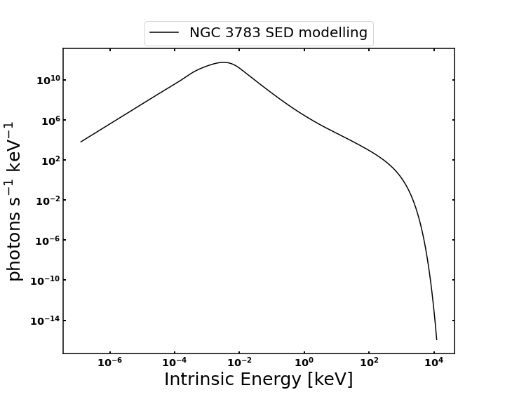
Figure 1: SED of NGC 3783 used in this work, based on Mehdipour et al. (2017) for the $2000-2001$ observation in an unobscured state.

2.2 Source simulated light curve

We use a doubly broken power spectral density (PSD, see Eq. 3) model to simulate the NGC $3783$ light curve (Markowitz, 2005),

$$P(f)=\begin{cases}A_{l},&f\leq f_{l},\\ A(f/f_{h})^{-1},&f_{l}<f\leq f_{h},\\ A(f/f_{h})^{-\beta},&f>f_{h},\end{cases}$$ (3)

where $A_{l}$ is the PSD amplitude below the low-frequency break $f_{l}=2\times 10^{-7}$ Hz, here the PSD has zero slopes. $A=A_{l}(f_{h}/f_{l})^{-1}$ is the PSD amplitude at the high-frequency break $f_{h}=4\times 10^{-6}$ Hz. We adopt the best-fit Monte Carlo results from Markowitz (2005) Table $2$ and set the slope value $\beta=2.6$ as well as the power amplitude $A=7200\,\rm Hz^{-1}$ to simulate the source light curve with variability in the energy band of $0.2-12$ keV. The range between $\rm 2.5\times 10^{5}\,s$ and $\rm 5\times 10^{6}\,s$ becomes the typical timescale where high fluctuation occurs.

Figure 2 shows that the relative root-mean-square fluctuations decrease significantly as the binning time (hereafter $t_{\rm bin}$) increases from $10^{5}$ to $10^{7}\rm\,s$, while the variations on timescale $\rm\leq 10^{4}\,s$ remain nearly constant. Therefore, we 1) sample the light curve with bin size of $\rm 10^{4}\,s$ and length of $\rm 10^{10}\,s$ or approximately $10^{6}\,t_{\rm bin}$, 2) and rebin the light curve to $10^{5}$ and/or $10^{6}\,\rm s$ bins for simulations with lower gas densities. For any densities of interest, the sampling time bin $t_{\rm bin}$ is shorter than the typical recombination timescale of the WA.

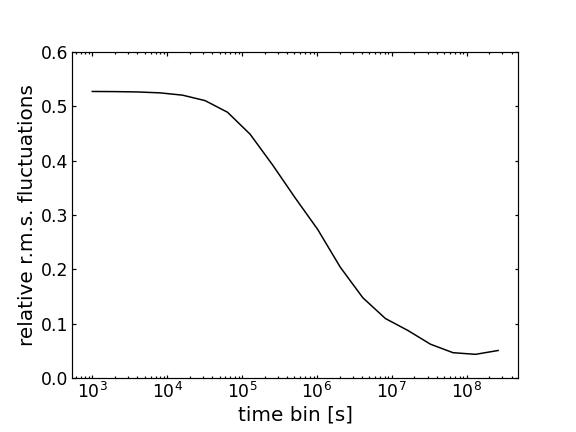
Figure 2: The relative root-mean-square of fluctuations for different binning time of NGC $3783$ based on Eq. 3.

2.3 10 WA components

We use the modelling based on the extensive observations with Chandra and XMM-Newton (Mehdipour et al., 2017). By analyzing the archival Chandra and XMM-Newton grating data taken in $2000$, $2001$ and $2013$ when the AGN was in an unobscured state, Mao et al. (2019) found $9$ photoionized absorption components with different ionization parameters and kinematics. We incorporate them as components $1-9$ in our current work. In the obscured state of the December $2016$ data, Mehdipour et al. (2017) find evidence of a strong high-ionisation component (abbreviation HC in their Fig. 4), which is designated as component $0$ in our present work. AGN SEDs do not normally change their shape a lot, unless there is strong X-ray obscuration, like in the above case. But the component $0$, due to its high-ionization state, is likely located near the center and therefore is not shielded by the obscurer. So it is reasonable to assume that both component $0$ and components $1-9$ experience the same unobscured SED.

Table 1 shows the parameters of the $10$ WA components obtained with the pion model of SPEX. We use them as initial conditions for our tpho calculations.

Table 1: The pion good-fit parameters of $10$ X-ray WAs components of NGC 3783 (see Mehdipour et al., 2017 Table 1 $\&$ Mao et al., 2019 Table 3). $N_{\rm H}$ is column density in unit of $10^{26}\,\rm m^{-2}$, $\rm log\xi$ is ionized parameter in logarithm scale. $v_{\rm out}$ is the outflow velocity, $\sigma_{v}$ is RMS velocity.

Comp	$N_{\rm H}$	log$\xi$	$v_{\rm out}$	$\sigma_{v}$
	[$10^{26}\,\rm m^{-2}$]	[nWm]	[$\rm km\,s^{-1}$]	[$\rm km\,s^{-1}$]
0	16	3.61	-2300	2500
1	1.11	3.02	-480	120
2	0.21	2.74	-1300	120
3	0.61	2.55	-830	46
4	1.24	2.40	-460	46
5	0.5	1.65	-575	46
6	0.12	0.92	-1170	46
7	0.015	0.58	-1070	46
8	0.007	-0.01	-1600	790
9	0.044	-0.65	-1100	790

2.4 Recombination timescale

Photoionization or recombination of the ionized gas in response to changes in the ionising continuum will occur. For each specific ion $X_{\rm i}$, the recombination timescale $t_{\rm rec}$ is the time that gas needs to respond to a decrease of the continuum. It depends on the local density and the ion population, following the equation (Bottorff et al., 2000, Ebrero et al., 2016):

$$t_{\rm rec}(X_{\rm i})=\left(\alpha_{r}(X_{\rm i})n_{\rm e}\left[\frac{f(X_{\rm i+1})}{f(X_{\rm i})}-\frac{\alpha_{r}(X_{\rm i-1})}{\alpha_{r}(X_{\rm i})}\right]\right)^{-1},$$ (4)

where $\alpha_{r}(X_{\rm i})$ is the recombination rate from ion $X_{\rm i-1}$ to ion $X_{\rm i}$, and $f(X_{\rm i})$ is the fraction of element $X$ at the ionization level $i$. The recombination rates $\alpha_{r}$ are known from atomic physics, and the fractions $f$ can be determined from the ionization balance of the source. $n_{\rm e}$ is the electron density.

For a cloud with known ionization structure, $t_{\rm rec}\propto 1/n_{\rm e}$. We show in Table 2 the column densities of the most relevant ions for each WA component, calculated using the model presented in Table 1 in an equilibrium state. Ebrero et al. (2016) use the ionic column densities of these most important ions to compute $n_{\rm e}\times t_{\rm rec}$, and they averaged the $n_{\rm e}\times t_{\rm rec}$ of all used ion to estimate it for the relevant WA component. The recombination timescale is defined this way through Eq. 4, however, changes sign near the ion with the highest relative concentration and becomes very large in the absolute value. This makes this definition of the recombination timescale not very useful.

Table 2: Ion column density $N_{\rm X}$ in $[10^{20}\,\rm m^{-2}]$ of the $10$ WA components for the specified Fe, S, Si, Mg, O, N ions. The results are obtained from our pion calculation and $N_{\rm H}$ and $\rm log\xi$ of Table 1 as the input value. For each component and each element, we show the column densities of the top three maxima abundance ions.

Comp 0 Comp 1 Comp 2 Comp 3 Comp 4 Comp 5 Comp 6 Comp 7 Comp 8 Comp 9 Z ion $N_{\rm X}$ Z ion $N_{\rm X}$ Z ion $N_{\rm X}$ Z ion $N_{\rm X}$ Z ion $N_{\rm X}$ Z ion $N_{\rm X}$ Z ion $N_{\rm X}$ Z ion $N_{\rm X}$ Z ion $N_{\rm X}$ Z ion $N_{\rm X}$ Fe 27 322.37 Fe 25 15.45 Fe 20 1.91 Fe 19 7.17 Fe 19 15.50 Fe 10 5.68 Fe 8 2.91 Fe 8 0.40 Fe 8 0.13 Fe 7 0.57 Fe 26 167.41 Fe 24 7.08 Fe 21 1.76 Fe 20 5.38 Fe 18 12.73 Fe 9 4.63 Fe 9 0.71 Fe 7 0.05 Fe 7 0.08 Fe 6 0.54 Fe 25 31.98 Fe 23 4.50 Fe 19 1.29 Fe 18 3.42 Fe 20 5.68 Fe 11 3.04 Fe 10 0.15 Fe 9 0.04 Fe 6 0.01 Fe 8 0.19 S 17 252.27 S 17 10.08 S 16 1.52 S 15 5.00 S 15 9.71 S 11 2.50 S 8 0.98 S 8 0.14 S 7 0.05 S 4 0.36 S 16 7.11 S 16 6.64 S 15 1.20 S 16 3.17 S 14 3.05 S 10 2.41 S 9 0.66 S 7 0.06 S 8 0.02 S 6 0.10 S 15 0.10 S 15 1.25 S 17 0.58 S 14 0.78 S 16 2.95 S 9 1.44 S 7 0.17 S 9 0.03 S 6 0.02 S 5 0.09 Si 15 609.58 Si 15 32.54 Si 14 3.68 Si 14 10.88 Si 13 23.76 Si 9 6.85 Si 8 2.57 Si 7 0.29 Si 6 0.12 Si 5 0.79 Si 14 7.14 Si 14 9.46 Si 15 3.11 Si 13 7.49 Si 14 16.42 Si 10 6.26 Si 7 1.45 Si 8 0.20 Si 7 0.10 Si 6 0.59 Si 13 0.05 Si 13 0.78 Si 13 1.26 Si 15 4.63 Si 15 3.39 Si 8 2.77 Si 9 0.41 Si 6 0.07 Si 5 0.03 Si 4 0.14 Mg 13 632.70 Mg 13 39.29 Mg 13 5.38 Mg 13 10.88 Mg 12 23.91 Mg 11 6.59 Mg 7 1.98 Mg 7 0.24 Mg 6 0.12 Mg 5 0.88 Mg 12 2.79 Mg 12 4.64 Mg 12 2.62 Mg 12 10.58 Mg 11 12.92 Mg 9 5.05 Mg 8 1.40 Mg 6 0.22 Mg 5 0.12 Mg 4 0.63 Mg 11 0.01 Mg 11 0.15 Mg 11 0.33 Mg 11 2.71 Mg 13 11.86 Mg 10 3.70 Mg 6 0.72 Mg 8 0.07 Mg 7 0.03 Mg 6 0.19 O 9 9682.56 O 9 665.86 O 9 122.21 O 9 341.28 O 9 638.38 O 8 153.22 O 7 47.82 O 7 4.19 O 5 1.62 O 4 17.14 O 8 2.81 O 8 6.04 O 8 4.87 O 8 27.52 O 8 108.38 O 7 89.37 O 6 12.09 O 6 2.67 O 4 1.37 O 3 4.61 – – – O 7 0.03 O 7 0.04 O 7 0.46 O 7 3.86 O 9 57.77 O 8 7.82 O 5 1.63 O 6 0.85 O 5 4.15 N 8 1306.38 N 8 90.32 N 8 16.87 N 8 48.22 N 8 94.58 N 7 19.21 N 6 6.25 N 6 0.85 N 6 0.20 N 4 1.83 N 7 0.14 N 7 0.32 N 7 0.27 N 7 1.59 N 7 6.59 N 8 17.44 N 7 2.75 N 5 0.17 N 5 0.17 N 3 1.14 – – – N 6 0.00 N 6 0.00 N 6 0.01 N 6 0.09 N 6 4.15 N 5 0.47 N 7 0.15 N 4 0.17 N 5 0.47

Table 3: Ion species recombination timescale $t_{\rm rec}$ and element charge time $t_{C}$ using pion calculation for WA component $0$ with $\rm log\xi=3.61$ as well as $n_{\rm H}=10^{10}\,\rm m^{-3}$.

WA component 0 of NGC 3783
ion	$t_{\rm rec}\,[\rm s]$	$t_{C}\,[\rm s]$
Fe XXVII	$-2.23\times 10^{7}$
Fe XXVI	$1.98\times 10^{7}$
Fe XXV	$6.17\times 10^{6}$	$2.45\times 10^{7}$
S XVII	$-8.13\times 10^{7}$
S XVI	$2.38\times 10^{7}$	$8.07\times 10^{7}$
Si XV	$-1.18\times 10^{8}$
Si XIV	$1.40\times 10^{6}$	$1.17\times 10^{8}$
Mg XIII	$-1.82\times 10^{8}$
Mg XII	$8.10\times 10^{5}$	$1.81\times 10^{8}$
O IX	$-6.00\times 10^{8}$	$5.99\times 10^{8}$

Hence we simply define the recombination time scale of an element by the time that the ionized plasma needs to change the average charge of the element by one charge state, namely:

$$t_{C}=\frac{1}{dC/dt}\,\,.$$ (5)

The average charge $C$ is defined by

$$C=\frac{\sum_{i=1}^{n}f(X_{i})\times(i-1)}{\sum_{i=1}^{n}f(X_{i})}\,\,,$$ (6)

and

$$\frac{dC}{dt}=\sum_{i=1}^{n}[f(X_{\rm i+1})\alpha_{r}(X_{\rm i+1})-f(X_{\rm i})\alpha_{r}(X_{\rm i})]i\,\,,$$ (7)

where the denotation of $f(X_{\rm i})$ and $\alpha_{r}(X_{i})$ are same as shown in the Eq. 4. Table 3 shows examples of $t_{\rm C}$ and $t_{\rm rec}$ where consistency between the two values can be seen. Following the above calculation, we replace the previous definition of $t_{\rm rec}$ by $t_{\rm C}$ to characterize the recombination timescale.

To quantity the relation between $t_{\rm C}$ and $n_{\rm e}$, we use the logarithm of their product using the following equation

$$\rm log(\it t_{C}\times n_{\rm e})=K(\xi,Z)\,\,,$$ (8)

where we express $t_{\rm C}$ in second and $n_{\rm e}$ in $\rm m^{-3}$. Table 4 shows the $K(\xi,Z)$ value for the 10 WA components from a pion calculation using Eq. 5 for Fe, S, Si, Mg, O, N.

Table 4: The quantity $K(\xi,Z)$ for the 10 WA components.

Comp	$K(\xi,\rm Fe)$	$K(\xi,\rm S)$	$K(\xi,\rm Si)$	$K(\xi,\rm Mg)$	$K(\xi,\rm O)$	$K(\xi,\rm N)$
0	17.39	17.91	18.23	18.26	18.78	18.95
1	16.58	17.22	17.33	17.47	17.91	18.06
2	16.10	16.96	17.25	17.18	17.57	17.71
3	16.13	16.80	16.99	17.11	17.46	17.59
4	16.13	16.40	16.77	16.98	17.30	17.42
5	15.31	16.06	15.98	16.23	17.00	17.08
6	15.74	16.29	16.22	16.22	16.71	16.94
7	16.02	16.47	16.42	16.30	16.60	16.84
8	16.43	16.56	16.71	16.52	16.55	16.68
9	16.70	16.63	16.94	16.84	16.76	16.73

2.5 TPHO calculation

We now apply the tpho model to calculate the time evolution of each WA component of NGC 3783. Starting point of the tpho calculation is an equilibrium solution which can be obtained from the pion model, ideally using the luminosity averaged over the entire simulation. Figure 3 shows the simulated light curve with a $t_{\rm bin}$ of $10^{4}$ s, $512$ data points resulting in a duration of $5.12\times 10^{6}\rm\,s$. The initial parameters, such as ionization parameter $\xi$ and column density $N_{\rm H}$, are taken from Table 1. We explore a range of hydrogen number density ($n_{\rm H}$) from $10^{8}\,\rm m^{-3}$ to $10^{15}\,\rm m^{-3}$.

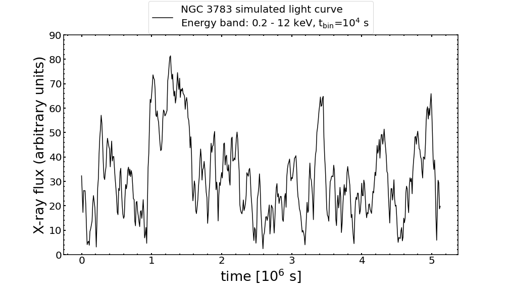
Figure 3: NGC 3783 simulated light curve in the $0.2-12$ keV band from the PSD shape of Markowitz (2005).

If the photoionized plasma is too far away from the nucleus and/or the density of the plasma is too low, the plasma is in a quasi-steady state with its ionization state varying slightly around the mean value corresponding to the mean ionizing flux level over time; whereas for high density the ion concentration will simultaneously follow the ionizing luminosity variation in a near-equilibrium state (Krolik & Kriss, 1995; Nicastro et al., 1999; Kaastra et al., 2012; Silva et al., 2016). Here we select the density range from $10{{}^{8}}\,\rm m^{-3}$ to $10^{15}\,\rm m^{-3}$ that encompasses the steady state, delayed state and nearby equilibrium state (see Sect. 3.1) as follows from our tpho calculation.

To further investigate the delayed state and to apply density diagnostics, it is needed to set up the simulation with the following conditions,

$$t_{\rm bin}<<t_{\rm var}(\sim t_{\rm C})<<t_{\rm tot}\,\,.$$ (9)

It is necessary to have $t_{\rm bin}<<t_{\rm var}$, which guarantees that the variability of the ionizing luminosity is sufficiently sampled. With $t_{\rm var}<<t_{\rm tot}$, each simulation run would then contain multiple ionization-recombination periods to get better constraints. As will be addressed below, significant lags between the outflows and the central source are likely to be observed when $t_{\rm var}$ approaches the recombination time $t_{\rm C}$.

To be specific, we use $t_{\rm bin}=10^{4},10^{5},10^{6}\,\rm s$ for density $10^{12},10^{11},10^{10}\,\rm m^{-3}$, respectively.

3 Results

We calculate the thermal stability curve of the $10$ WA components by computing the temperature for a range of $\xi$ values using the pion model made with our SED. From this, we determine the pressure ionization parameter, the ratio of radiation pressure to gas pressure, $\Xi$ defined as (Krolik et al., 1981)

$$\Xi=L/4\pi r^{2}cp=\xi/4\pi ckT\,\,.$$ (10)

The shape of this curve in general depends on the precise form of the incoming X-ray spectrum. In this equation, $p$ is the gas pressure, $c$ is the speed of light, $k$ is the constant of Boltzmann, and $T$ is the electron temperature. Figure 4 shows a plot of $\rm log\it T$ versus $\rm log\Xi$. Note that in general for a single value of $\Xi$ more temperature solutions are possible (in particular when log$\Xi$ is close to $1$). Only solutions with $dT/d\Xi>0$ are stable. Hence it seems that components $1$ and $4$ are in an unstable state.

Figure 4: The electron temperature in $\rm log\it T$ versus pressure ionization parameter in $\rm log\Xi$ (”S” curve in black). The colored dots show the $10$ X-ray WA components.

Using the light curve described in Sect. 2.2 and the SED described in Sect. 2.1, we apply the tpho model for a range of densities for each WA component. The ion concentration is changing over time because the gas ionises when the flux rises, and recombines when the flux goes down. The recombination is responsible for the lag between the light curve and the ion concentration variability. We also investigate the relationship between density and lag time scales to further characterize this phenomenon. Here we present the Component 0 results in more detail as an example.

3.1 Delayed state in ion concentration

Due to its high ionization state, Component $0$ predominately produces absorption lines in the Fe-K band, hence we focus on Fe. We use the light curve with $t_{\rm bin}=10^{4}\,\rm s$ for the density ranging from $10^{8}\,\rm m^{-3}$ to $10^{15}\,\rm m^{-3}$ in this section.

Fig 5 shows the ion concentrations of the most importannt Fe ions and the temperature as a function of time for three different densities. When the luminosity increases, the Fe XXVII concentration increases, of the expense of Fe XXIV - Fe XXVI due to conservation of the total number of Fe nuclei.

For a density of $1\times 10^{12}\,\rm m^{-3}$, the Fe XXVII ion concentration shows clear lag with respect to the light curve. The lag arises mainly from the recombination timescale of the plasma, which depends inversely on the density (see Eq. 4). Therefore with increasing density, the Fe XXVII ion concentration (from blue, red to orange curve) will correspond to smaller lag timescale. For a higher density of $1\times 10^{14}\rm\,m^{-3}$ , the variability of Fe XXVII becomes well synchronized with the light curve. That is also the reason why the ion concentrations show smoother appearance from high to low density. And the standard deviation amplitude of Fe XXVII for $10^{10},10^{12},10^{14}\,\rm m^{-3}$, is $0.007$, $0.14$ and $0.27$ respectively.

In Fig. 5, the last panel shows the time-evolved electron temperature $T$ profile. For low density, e.g. $10^{10},10^{12}\,\rm m^{-3}$, there are no variations and the temperature is constant over time, because cooling rate almost equals the heating rate within the duration of the light curve. For higher density, e.g. $10^{14}\,\rm m^{-3}$, the electron temperature lags due to the cooling time $\sim 10^{6}\,\rm s$. Both time dependencies of the ion concentration and electron temperature are in agreement with Rogantini et al. (2022) (see their Figure $7\,\&\,8$).

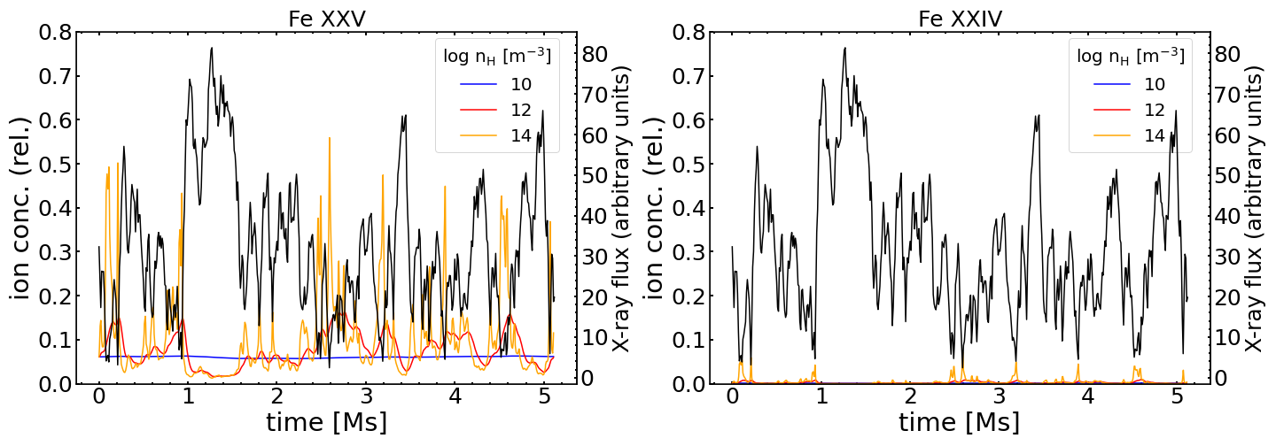
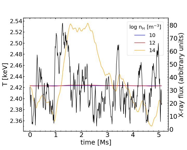
Figure 5: The tpho calculation of the X-ray WA component $0$ of NGC $3783$ based on the simulated light curve (Fig. 3) and SED (Fig. 1). The time-dependent ion concentration of Fe XXVII, Fe XXVI, Fe XXV, Fe XXIV are shown for hydrogen number density of $\rm 10^{10},10^{12},10^{14}\,m^{-3}$ in blue, red and orange, respectively. The last figure shows the electron temperature $T$ of the plasma of Component $0$ as a function of time.

3.2 Density-dependent lag

The lag between the ionizing luminosity and ion concentration as shown in Fig. 5 is caused by delayed recombination. To quantify the lag in our current work, we determine the cross-correlation function (CCF) between the average charge of Fe and the ionizing luminosity as shown in Fig. 6. The Fe average charge $C_{\rm Fe}$ is derived using Eq. 6 for each time bin. The ionizing luminosity $L$ is also the value for each time bin. For both quantities, we calculate the relative variation by subtracting the long-term average. The CCF is a measure of the similarity of two series as a function of the displacement of one relative to the other as shown in the following equation:

$$((L-\overline{L})*(C-\overline{C}))[\Delta t]=\sum_{-\infty}^{\infty}\overline{(L-\overline{L})[t]}(C-\overline{C})[t+\Delta t]\,.$$ (11)

$\Delta t$ is defined as the displacement, also known as the lag. We compute the CCF using the procedure of the website of Scipy-correlation between the quantity $(C_{\rm j}-\overline{C})_{\rm Fe}$ and mean-subtracted ionizing luminosity ($L_{\rm j}-\overline{L}$). $\overline{C}$ and $\overline{L}$ here are the average value calculated from all bins. We take the lag value corresponding to the largest correlativity for each calculation (see red curve at the bottom of Fig. 6).

Figure 6 shows the CCF for a hydrogen number density of $10^{12}\,\rm m^{-3}$ and component 0. We see here a lag timescale of $5\times 10^{4}\,\rm s$ (16 hours or more than half a day) for a density of $\rm 10^{12}\,m^{-3}$. There are lag timescale of $1\times 10^{6},2\times 10^{5}\,\rm s$ for the density of $10^{10},10^{11}\,\rm m^{-3}$, respectively. The uncertainties in the simulated light curve, derived from the power spectral density of Markowitz (2005), can introduce errors in the lag measurement. To account for this, we perform re-simulations of the light curves by considering the errors in the observed PSD. By comparing the resulting lag times obtained from different light curves, we determine an uncertainty of roughly $10\%$.

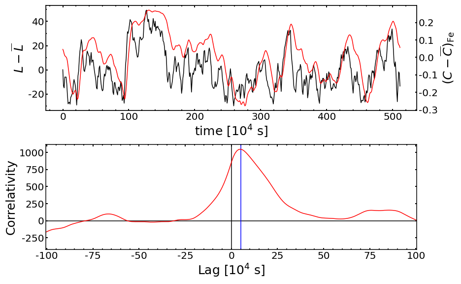
Figure 6: Cross correlation of the Fe average charge with ionizing luminosity for Component 0 of NGC $3783$. Top panel: Fe mean-subtracted average change (red curve) from tpho calculation with hydrogen number density of $\rm 10^{12}\,m^{-3}$, and with ionizing luminosity in black ($t_{\rm bin}=10^{4}\,\rm s$). Bottom: cross correlation versus lag. The blue vertical line marks the lag timescale of $5\times 10^{4}\,\rm s$ corresponding to the largest correlation.

The lag timescale in our work detected by the CCF method is the net effect of the recombination and ionization periods. Similar to $t_{\rm rec}\sim 1/n$, the lag timescale decreases with increasing hydrogen number density due to the shorter recombination timescale as shown in the top panel of Figure 7. We fit these three data points (see black dot line) with a power law

$$t_{lag_{\rm Fe}}=10^{b}\times n_{\rm H}^{k}\,,$$ (12)

and find $\rm k=-0.651$ and $\rm b=12.489$. Here, we find for Component 0, $t_{lag_{\rm Fe}}\varpropto 1/n_{\rm H}^{0.651}$. The observed lag, which is a result of both recombination and ionization, is described by a power index of less than $1$. We take here as a typical minimum useful lag the time scale of $\rm 10^{4}\,s$, which is approximately the timescale necessary for relevant AGN observations, i.e. the time needed to obtain a spectrum with sufficient quality.

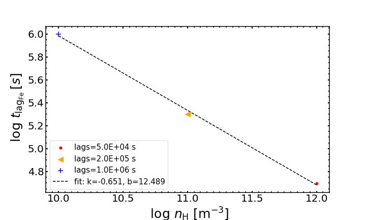
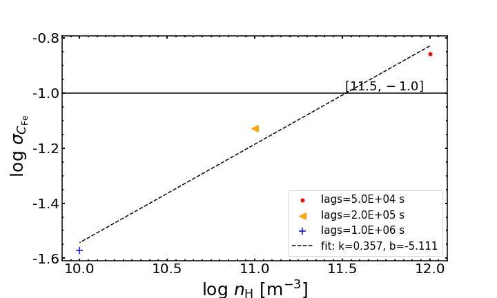
Figure 7: Top: The relation of lag timescale vs. hydrogen number density based on Fig. 6 for Component $0$. Bottom: The relation of $\sigma_{C}$ for Fe vs. density for Component $0$.

To scale the amplitude to the mean-substracted average charge, we use root-mean-square $\rm\sigma_{C}=\sqrt{\frac{\sum_{j=1}^{j=n}(C_{\rm j}-\overline{C})^{2}}{n}}$, where $C_{\rm j}$ means average charge in the $j^{\rm th}$ time binsize and $n$ means the numbers of time bins. Hence, for each calculation from tpho, we further calculate the $\rm\sigma_{C}$ of the Fe ion concentration. At the bottom of Figure 7, we show the relation between $\sigma_{C}$ of Fe and hydrogen number density. We find that relatively high density corresponds to a relative large $\sigma_{C}$ value, as well as a shorter lag time. We fit these three data points (see black dot line) with a power-law

$$\sigma_{C_{\rm Fe}}=10^{\rm b}\times n_{\rm H}^{\rm k}\,,$$ (13)

and find $\rm k=0.357$ and $\rm b=-5.111$. We assume that we can observe in practice significant change in absorption line spectra where $\sigma_{C_{\rm Fe}}>0.1$; as for lower densities or longer lags, the amplitude of the charge variations become practically too small for effective measurement. $10\%$ serves as an empirical standard. A $10\%$ change in average change for one element corresponds typically to changes of order $10\%$ in the ion concentration and hence ionic column densities and line optical depth. This is approximately true based on the observed Fe ion concentrations reported in Kaspi et al. (2002). For component $0$, for Fe, we find a density of (about) $\rm 3\times 10^{11}\,m^{-3}$ (see the black horizontal line) when $\sigma=0.1$.

From the constraints of lag larger than $10^{4}\,\rm s$ and $\sigma_{\rm C}$ larger than $10\%$, for component $0$ and Fe, lags can be detected for densities roughly between $3\times 10^{11}$ and $\rm 1\times 10^{13}\,m^{-3}$.

Hence, the above method, dubbed here, tpho-delay method, can be used to constrain the density range of the outflowing wind when the source variability timescale is comparable to the recombination time, i.e. ionized plasma in delayed state. The same calculation has been carried out for the other $9$ components.

3.3 Constraint on the WA density

Apart from the constraint that can be obtained from the spectral-timing analysis, i.e. tpho-delay method of Section 3.2 in our current work, we take into account other astrophysical conditions. A lower limit to the density is obtained by assuming that the thickness ($\Delta r$) of the WA plasma can not exceed its distance ($r$) to the SMBH (Krolik & Kriss, 2001; Blustin et al., 2005), namely $\Delta r\leq r$, so we can derive the lower limit of the physical density by:

$$n_{\rm H,low}=\frac{\xi\times N_{\rm H}^{2}}{L}\,,$$ (14)

where $N_{\rm H}$ is the column density.

The upper limit to the density can be obtained based on the assumption that the outflow velocity $v_{\rm out}$ of the wind is larger than or equal to the escape velocity ($v_{\rm esc}=\sqrt{2GM_{\rm BH}/r}$ ), e.g. Blustin et al. (2005). It gives,

$$n_{\rm H,upp}=\frac{L\times{v_{\rm out}^{4}}}{{4\times(G\times M_{\rm BH})^{2}}\times\xi}\,,$$ (15)

Using $M_{\rm BH}=3\times 10^{7}\,M_{\sun}$ (Vestergaard & Peterson, 2006) and other parameters from Table 1, we compute $n_{\rm H,low}$ and $n_{\rm H,upp}$.

Following the technique introduced in Mao et al. (2017), we calculate the ranges of detectable densities using absorption lines from meta-stable levels in C- like ions for NGC $3783$. The parameter range covered by this method exhibits dependence on ionization parameter and density, as depicted in the colored rectangles of Figure 8.

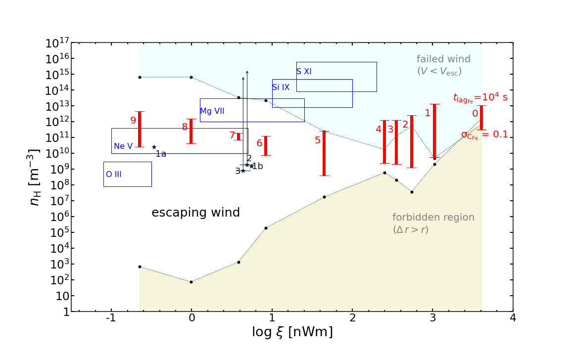
Figure 8: The detectable density ranges of $10$ X-ray WA components in the unobscured state of NGC $3783$. The $10$ WAs are marked in red. Upper black points and line: outflow velocity equals the escape velocity. For higher densities, winds cannot escape i.e. they are failed winds as shown in the light azure shaded region. Lower black points and line: the thickness of the wind equals its distance to the core. For lower densities, no solution exists, i.e. forbidden region shown in the yellow region. Red vertical solid lines: the detectable density range by the tpho-delay method for all $10$ X-ray WAs. The upper limit: lag equals $10^{4}\rm\,s$. For higher densities, lags are shorter and more difficult to measure due to photon statistics. The lower limit: relative variations of the charge of Fe ions is $10\%$. For lower densities, variations become too small to measure. Navy stars and lines with labels $1a$ to $3$: density measurements or lower limits from Gabel et al. (2005). $\xi$ values converted for models with the SED of Mehdipour et al. (2017). Rectangular boxes: regions where density-sensitive X-ray lines can be used to measure densities.

Figure 8 shows a comprehensive constraint on the density ranges for all 10 WA components as derived from the methods described above.

The margins for a failed wind and the forbidden region obtained based on previous observations present the upper and lower limits density for $V=V_{\rm esc}$ and $\Delta r=r$, respectively. For X-ray component $0$, we find that $10^{12.2}<n_{\rm H}<10^{11.8}\,\rm m^{-3}$ i.e. the lower limit is higher than the upper limit. It means that perhaps X-ray component $0$ is a candidate for a failed wind.

We see that for the components with a relatively narrow physical density range as well as higher ionization parameters, such as components $1-4$, the tpho-delay method provides powerful diagnostics for the failed wind scenario. The detectable density range of the tpho-delay method for these components $2-5$ covers most of their available physical density range, hence their density can be determined well using our method. Starting from component $5$, metastable density works, Si IX and S XI can diagnose whether component $5$ is failed wind or not.

For components $6-9$ with a relatively broad allowed physical density range and a low ionization parameter, we can combine the tpho-delay method with metastable C-like ions to give density constraints in the X-ray band. For components $7-9$, we can have a cross-check between tpho-delay and the Ne V metastable lines. Mg VII and Ne V as well as O III metastable lines also expand the detectable density range for components $6-9$.

Gray stars and lines represent the density measurements or lower limit from UV observations using the UV metastable absorption lines (Table $3$ in Gabel et al., 2005). Their ionization parameter $U_{\rm H}=Q_{\rm H}/4\pi cn_{\rm H}r^{2}$ was converted into $\xi$ for the models with the SED and luminosity of Mehdipour et al. (2017). We will discuss UV components further in Section 5.

We note that here we use $t_{lag_{\rm Fe}}$, the lag timescale of the Fe average charge, to give the detectable density range for components at different ionization states. However, the other elements would complement Fe in particular for the low ionization components. To fully comprehend the behaviour of the WA outflows, we will need to conduct similar calculations for other critical elements, such as C, O, N, Mg and Si, among others.

3.4 TPHO vs. PION

Figure 9: Ionization parameter and Fe ion average charge comparisons for tpho and pion for X-ray WA component $0$ of NGC $3783$ for three different densities ($10^{10},10^{11}$ and $10^{12}\,\rm m^{-3}$ from top to bottom). In the left panels: the black dots represent the $\xi$ values of pion that are needed to obtain are the same Fe average charge as for the tpho model. $\xi_{\rm TPHO}$ is a luminosity-dependent quantity in tpho calculations (See Eq. 16). The red line represents the condition where the $\rm log\xi$ from pion is equal to tpho. The right panels show $\rm log\xi$ versus $C_{\rm Fe}$, where the blue dots represent the pion $\rm log\xi$ and red dots represent the tpho $\rm log\xi$ respectively.

In our current work, we derive the density of ionized plasma using the tpho model. In tpho calculations, the $\rm\xi$ value simply scales with the time-dependent luminosity value, assuming that the product $n_{\rm H}\times r^{2}$ remains constant over time. Thus,

$$\xi_{\rm TPHO}(t)\equiv\frac{L(t)}{L_{\circ}}\times\xi_{\circ}\,,$$ (16)

where $L_{\circ}$ and $\xi_{\circ}$ are the luminosity and ionization parameter at $t=0$, which is assumed to be in equilibrium state.

The pion model assumes photoionization equilibrium, and the ionization parameter $\rm\xi$ is obtained by fitting the observed spectra. Once the $\rm\xi$ value is known, the ion concentrations of different elements are known and the corresponding elemental average charge is also determined. So there is a one-to-one relation of $\xi_{\rm PION}$ to the element average charge in the pion equilibrium state.

In the left panels of Figure 9, the black dots represent the $\xi$ values of the pion model that are needed to yield the same Fe average charge value as the $C_{\rm Fe}(t)$ from the tpho simulation, represented by $\xi_{\rm TPHO}(t)$. The red line corresponds to equal values of both quantities. Only a small fraction of data points are located on the red line, which corresponds to the equilibrium state.

This figure also shows the limitations of applying an equilibrium (pion) model to a source that in reality has time-dependent photoionization, as represented by the realistic tpho model. This holds in particular for periods of low luminosity (low $\xi_{\rm TPHO}(t)$). In the right panels of Fig. 9, for example, $n_{\rm H}=10^{12}\,\rm m^{-3}$, the data point with the lowest $\xi_{\rm TPHO}$ value of $2.75$ (in the log) has an average charge for Fe of $25.4$; if the corresponding spectrum would be fitted with an equilibrium pion model, this average charge would yield $\rm log\xi=3.5$, a $\xi$ value that is $5.6$ times larger than the tpho value. Because the observer would like to use the measured luminosity for this data point to derive the product $n_{\rm H}\times r^{2}=L_{\rm ion}/\xi$, both the lower $L$ and larger $\xi$ would lead to an underestimate of $n_{\rm H}\times r^{2}$ by more than an order of magnitude.

4 Discussion

4.1 NGC $3783$ $10$ WAs geometry distance

We use the Eq. 2 to derive the detectable distance based on our lag density relation in current work and compare it with the NGC $3783$ intrinsic structure measured by GRAVITY Collaboration et al. (2021) as shown in Fig. 10. Component $0$ exhibits a detectable distance very close to the broad line region, while components $1-2$ can be constrained within the host dust structure. Component $1-4$ shows a relatively large detectable distance range, typically within or around $1$ parsec, which corresponds to the torus structure. Additionally, the distances of components $5-9$ are detectable with our method only when they locate outside the torus.

Figure 10: NGC $3783$ $10$ WAs predict detectable distance range with tpho-delay method in colored dash line. The vertical dash line are main components of structure measured by GRAVITY Collaboration et al. (2021).

4.2 Correspondence with the UV-X-ray absorbers

In addition to the $10$ X-ray WAs, there are absorbers detected in UV (Kraemer et al., 2001; Gabel et al., 2005) that exhibit a bit of common features as the chosen X-ray counterpart. Figure 8 shows three UV absorbers reported in Gabel et al. (2005), in which the component $1$ is composed of two physically distinct regions ($1a$ and $1b$) detected by the difference in covering factor and kinematic structure. It denotes that both components $1a$ and $1b$ are assumed that they are colocated based on a decrease in radial velocities of lines in both components together with the same outflowing velocity (bottom panel of Fig. 11), while the ionization parameter for component $1b$ derived in the unsaturated red wing of C IV and N V is higher than that of $1a$, and therefore component $1b$ has lower density and column density (top panel of Fig. 11). The electron density of the lower ionization component $1a$, $\sim 3\times 10^{10}\,\rm m^{-3}$, obtained directly from the individual meta-stable levels, falls in the range where the tpho-delay method, as well as the metastable lines of Ne V, can provide useful constraints. Moreover, UV component $1a$ appears to be intimately linked to the component $9$ in the X-ray. Therefore, UV component $1a$ can serve as a calibration for density diagnostic using an X-ray detector.

UV components $2$ and $3$ do not have direct estimates of the density and thus are less well constrained than component $1$ (Fig. 8). The lower limits on their densities are derived based on the basis of the observed variability. The ionization parameters from higher ionization UV absorbers, components $1b$, $2$, and $3$ with $\rm log\xi\sim 0.7$, are close to the X-ray component $7$ with $\rm log\xi\sim 0.6$. Nevertheless, the latter has a smaller total column density (Fig. 11).

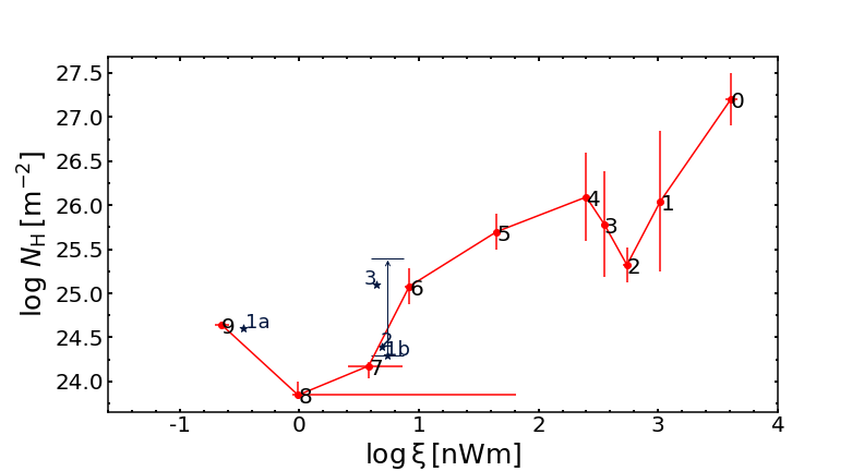
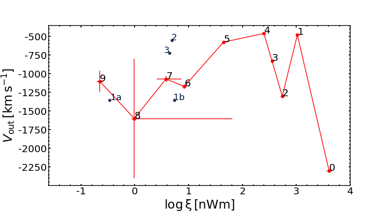
Figure 11: The $10$ X-ray WA components and $4$ UV components (Gabel et al., 2005) in NGC $3783$ observations. Top panel: $N_{\rm H}$ versus $\rm log\,\xi$. Bottom panel: $V_{\rm out}$ versus $\rm log\xi$.

Although the hints mentioned above suggest a possible connection between the UV absorbers and the lowly ionized X-ray counterparts, it is not yet established due to poor X-ray constraints. This hypothesis can be addressed through the high-resolution X-ray data that will be obtained with the upcoming XRISM (XRISM Science Team, 2022) and Athena missions (Nandra et al., 2013).

4.3 Crossing time

X-ray variability from black holes is generally characterized as a red noise process (Uttley et al., 2014), which can be contributed by different physical radiation processes (Cackett et al., 2021). Gabel et al. (2003) note that the observed changes in the absorption components could be due to the transverse motion of the clumping wind that moves across the line of sight, except for the intrinsic luminosity variability. To determine the potential impact of Keplerian motions on WA variability, we have calculated the crossing time of outflows and compared them with the recombination time.

The X-ray emitting region has a scale no larger than $20$ gravitational radii (Reis & Miller, 2013) as shown in the following equation,

$$s=\frac{20*G*M_{\rm BH}}{c^{2}}\,\,.$$ (17)

Therefore the crossing time $t_{\rm cross}$ can be computed,

$$t_{\rm cross}=\frac{s}{V_{\rm kepler}}\,\,,$$ (18)

where $V_{\rm kepler}=\sqrt{\frac{G\times M_{\rm BH}}{R_{\rm WA}}}$. Substituting Eq. 2 and Eq. 17 into Eq. 18, we come to,

$$t_{\rm cross}=\frac{20}{c^{2}}\,(G\times M_{\rm BH})^{1/2}\,(\frac{L_{\circ}}{\xi_{\circ}})^{1/4}\,n_{\rm H}^{-1/4}\,\,.$$ (19)

Here $L_{\circ}=6.36\times 10^{36}\,\rm W$ (Mehdipour et al., 2017), $\xi_{\circ}$ from Table 1.

The three timescales in Fig. 12, charge time $t_{C_{\rm Fe}}$, lag timescale $t_{lag_{\rm Fe}}$, crossing time $t_{\rm cross}$, are density-dependent. We also present the positions of density constraints from tpho-delay and other methods.

It shows that the density ranges where our tpho-delay method can offer useful constraints likely satisfy $t_{C_{\rm Fe}}<t_{\rm cross}$. This indicates that the transverse motion of the outflows could not have a significant impact on the density diagnostics obtained assuming luminosity variation, i.e. the ionization variation is mainly/likely caused by the variability, not the transverse motions. Hence, we consider the tpho-delay methods to be largely valid, even when accounting for the potential variability driven by motion.

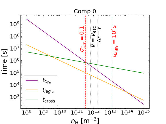
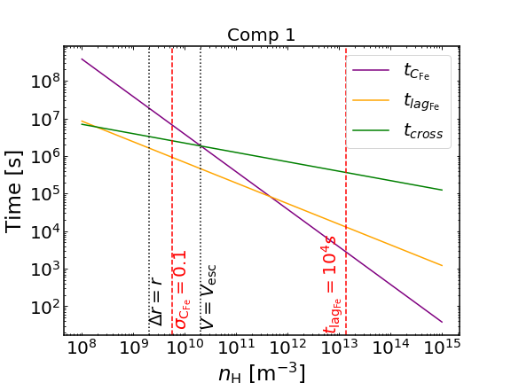
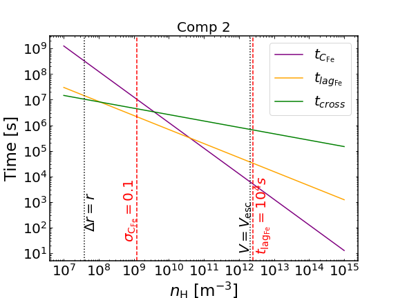
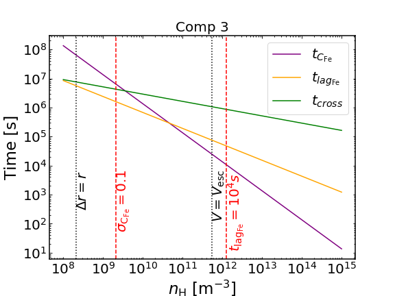
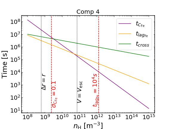
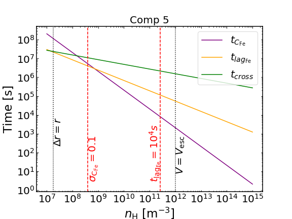
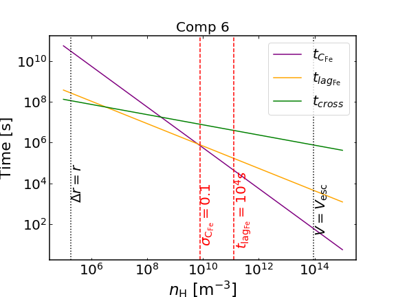
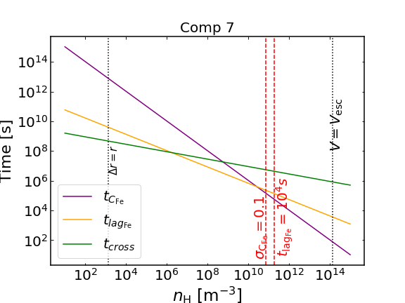
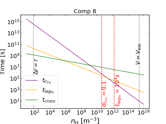
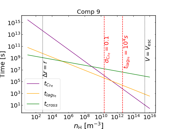
Figure 12: Comparing $t_{C_{\rm Fe}}$, $t_{lag_{\rm Fe}}$ and $t_{\rm cross}$ of NGC 3783 10 X-ray WAs. The dash and dot lines notations same as Fig.8.

4.4 SED and light curve of NGC 3783

The AGN SEDs do not normally change their shape a lot unless something dramatic happens: like in changing-look AGN where the accretion rate and the X-ray corona emission decline. Or if there is strong X-ray obscuration, and the difference between the impact of obscured and unobscured SED on the ionization state is significant, as shown in NGC $5548$ (Mehdipour et al., 2016). Here, the SED we used is uniformly derived from an unobscured state to study the $10$ WA components ionization state. Because the component $0$ is in the obscured state but not shielded by the obscurer, it is reasonable to assume that the same SED can be used for component $0$ and components $1-9$. NGC $3783$ is a Seyfert-$1$ galaxy without extreme changing-look accretion events observed until now. So it is reasonable to say that it is the normalization that is mostly changing in an unobscured state. Of course, individual SED components (like the soft excess) show some special variability, but usually this does not cause the shape to change too much such that it would impact photoionization. Thus for tpho to assume that only the normalization of the SED is changing is a good enough approximation in this case. We also note that deriving the variability of the SED shape (with limited data) has its challenges and assumptions which are highly model dependent.

4.5 Comparison with other time-resolved analyses

Time-dependent photoionization modelling for outflowing winds has been described in other papers, but with different model constructions. Silva et al. (2016) and Juráňová et al. (2022) carry out time-dependent photoionization modeling using pre-calculated runs from Cloudy, assuming equilibrium conditions. The tpho model Rogantini et al. (2022) however takes into account non-equlibrium state conditions and tracks the time-dependency of the heating and cooling process according to the lightcurve of the ionizing SED.

We point out that, without considering the non-equilibrium time-dependency of heating and cooling process, to some extent, it will affect the resulting calculation of ion concentration, because recombination rates are not only a function of density but also temperature. A long light curve history is required for tpho input, and the upcoming new satellite XRISM can provide good spectra to compare with the models. It is expected that tpho can be used to fit the observational data in the case that AGNs SED do not change their shape too much.

5 Conclusions

By utilizing a realistic SED with variability from a realistic PSD, and WA physical parameters based on previous X-ray observations, we performed a theoretical tpho model calculation to investigate the time-dependent photoionization plasma state of 10 WA components of NGC 3783. We have employed cross-correlation calculations to measure the correlation between response lag time and the outflow density for all WA components. By doing so, we have determined the ranges of density for which the tpho model can yield practical constraints, and we have compared our results with those obtained from metastable absorptions lines in X-ray and UV bands. We further prove that the Keplerian motion would have negligible impact on the density measurement for our range of interest. It is expected that our technique will be applied to the new data obtained with upcoming X-ray missions including XRISM and Athena.