Dynamic Residual Classifier for Class Incremental Learning

Abstract

The rehearsal strategy is widely used to alleviate the catastrophic forgetting problem in class incremental learning (CIL) by preserving limited exemplars from previous tasks. With imbalanced sample numbers between old and new classes, the classifier learning can be biased. Existing CIL methods exploit the long-tailed (LT) recognition techniques, e.g., the adjusted losses and the data re-sampling methods, to handle the data imbalance issue within each increment task. In this work, the dynamic nature of data imbalance in CIL is shown and a novel Dynamic Residual Classifier (DRC) is proposed to handle this challenging scenario. Specifically, DRC is built upon a recent advance residual classifier with the branch layer merging to handle the model-growing problem. Moreover, DRC is compatible with different CIL pipelines and substantially improves them. Combining DRC with the model adaptation and fusion (MAF) pipeline, this method achieves state-of-the-art results on both the conventional CIL and the LT-CIL benchmarks. Extensive experiments are also conducted for a detailed analysis. The code is publicly available.

1 Introduction

Deep models are prone to forgetting previously learned knowledge when sequentially fine-tuned on different tasks. Severe performance degradation on the old tasks can be observed. It is also known as catastrophic forgetting [17, 18]. Class incremental learning (CIL) methods [9, 35] aim to handle this issue and equip deep models with the capacity to continuously learn new categories without forgetting the old ones. The rehearsal strategy [37, 49, 38, 42, 44] has been widely used to achieve this goal. Specifically, a limited amount of exemplars from previous tasks are stored in a memory buffer and replayed when learning new tasks.

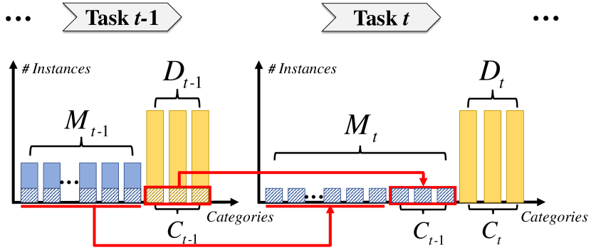
Figure 1: Data imbalance of CIL. With the exemplars of previous tasks buffered, the training data within each task is imbalanced. As the task increment proceeds, more categories appear in a fixed-size memory. Such imbalance becomes more severe.

Due to the relatively small size of the memory buffer, the training samples of a new class are far more than the old ones. Therefore, adopting the rehearsal strategy can introduce the data imbalance problem to CIL. Two kinds of long-tailed recognition techniques, the adjusted losses [36, 8] and the data re-sampling [28], are exploited by many CIL methods [25, 42, 3, 44] to learn the classifier with less bias. These methods alleviate the data imbalance within each increment task independently.

However, the data imbalance in CIL is dynamic and becomes more extreme as the task increment proceeds, as illustrated in Fig. 1. A novel dynamic residual classifier (DRC) is proposed in this work to handle this challenging scenario. Inspired by the recent advance residual classifier (RC) [7], a lightweight branch layer is inserted before the classifier to encode the task-specific knowledge. This new architecture enables the residual fusion of classifier outputs to alleviate the data imbalance effectively. However, directly applying RC for CIL leads to the model-growing problem, i.e., the growing overhead from the additional branch layers assigned to the new tasks. The proposed DRC handles this dynamic increment issue via the simple yet effective branch layer merging.

DRC is directly applicable to different CIL pipelines by simply replacing the fully connected (fc) classifiers. Three typical CIL pipelines, i.e., the Model Direct Transfer (MDT) [37, 15], the Model Expansion and Compression (MEC) [42, 44] and the Model Adaptation and Fusion (MAF) [24, 5], as shown in Fig. 2, are chosen to be combined with DRC. They can consistently benefit from such combinations, with clear improvements observed. The details and comparisons on such combinations are given in Sec. 3.3. More importantly, DRC is most compatible with MAF among the three pipelines. The resulting MAFDRC method achieves state-of-the-art performance under both conventional CIL and long-tailed CIL (LT-CIL) settings. Extensive analyzes are conducted to provide insights into each part. The main contributions are three-fold:

• We show the data imbalance issue in CIL rehearsal is dynamic across tasks rather than static within each task. The proposed dynamic residual classifier (DRC) aims to handle this challenging scenario from the perspective of classifier architecture, which is complementary to existing efforts in CIL;

• The branch layer architecture and residual fusion mechanism from a recent long-tailed classifier (RC) [7] are adopted by DRC to alleviate the negative impact of data imbalance on CIL for the first time. More importantly, the model-growing problem of the vanilla RC under the CIL setting is handled with the simple yet effective branch layer merging in DRC;

• The proposed DRC is generalizable. On the one hand, incorporating DRC brings clear improvements to different CIL pipelines. On the other hand, the effectiveness of DRC is demonstrated in both the CIL and the LT-CIL settings.

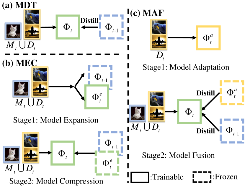
Figure 2: Illustrations of three CIL pipelines. (a) is the Model Direct Transfer (MDT). (b) depicts the Model Expansion and Compression (MEC). (c) shows the Model Adaptation and Fusion (MAF). $\Phi_{t}$ indicates the classification model of task $t$. $D_{t}$ and $M_{t}$ represent the new data and memory data of task $t$ respectively. Blue indicates old knowledge, yellow indicates new one and green represents a mixture of both.

2 Related Work

Class Incremental Learning (CIL) is one of the major settings in continual learning [41, 10]. It aims to equip deep models with the capacity to continually learn from a sequence of tasks with disjoint classes and avoids the Catastrophic Forgetting [17] of previously learned knowledge. Rehearsal-based methods  [37, 34, 49, 43, 38, 27] preserve very limited exemplars from previous tasks and replaying them in the new task to defy forgetting. Exemplars are selected by different strategies. iCaRL [37] stores a subset of samples per class by selecting the good approximations to class means in the feature space. RWalk [4] selects exemplars with higher entropy or those close to the classification boundary. Instead of storing raw data samples, DGR [40] exploits the synthetic instances from a generative model [19]. In this work, we use the rehearsal strategy as in [37]. The data imbalance caused by limited rehearsal memory is a challenge for Classifier Learning in CIL. To learn a less biased classifier, the adjusted losses [36, 8] are exploited by existing CIL methods. A margin ranking loss proposed by [25] encourages the old and new classes to be better separated and avoid ambiguities. The adjusted classification loss of FOSTER [42] aims to re-balance the logits of the rare (old) and dominant (new) classes. Based on a balanced training subset sampled [28], an independent classifier learning stage is introduced to alleviate the impact of data imbalance. For example, EEIL [3] finetunes its classifier while DER [44] trains a new one from scratch with such balanced data. Moreover, different post-hoc corrections are applied to the classifiers learned from the imbalanced data. The output logits of the new classifier are rescaled by a simple affine function in BiC [43]. The norms of the classifier weight vectors for the new and old classes are aligned in WA [49]. The proposed dynamic residual classifier (DRC) aims to handle the data imbalance of CIL with a new classifier of dynamic architecture. Therefore, it is complementary to the relevant CIL methods mentioned above.

Besides the rehearsal strategy, distillation techniques [23, 48] are used by different CIL pipelines to transfer the discriminative knowledge of preceding categories from the old models to the new ones, resulting in the Distillation-based methods [37, 15, 42, 24, 5]. Under the Model Direct Transfer (MDT) pipeline, the model is finetuned with both the new data and the distilled knowledge from the retained old model. The changes in attention maps between the new and old models are penalized via distillation in LwM [13]. Distillation also can be conducted on the prediction scores [37] or spatial features [15]. The Model Expansion and Compression (MEC) pipeline consists of two stages. In the first stage, the old model is retained and expanded with new modules for the learning of a new task. Such a model expansion stage is also known as the parameter isolation methods [32, 26, 44, 42, 16]. The feature representations from the old frozen model and the newly added one are concatenated and trained on the new task, as in DER [44] and FOSTER [42]. A dynamic model expansion strategy based on the ViT architecture [14] is proposed in DyTox [16]. In the next stage, the model compression, e.g., distillation [23] or network pruning [39], is applied to control the size of the expanded model. Under the Model Adaptation and Fusion (MAF) pipeline, a model optimized on the new task only is obtained at the adaptation stage. The new knowledge within this adapted model together with the old knowledge from either the exemplars [24] or the old model [5] are integrated into a single model via distillation. A neural network is split into two partitions in [30] for training the new task separated from the old task and reconnecting them to fuse the knowledge across tasks. The proposed DRC is compatible with the three pipelines and clearly improves their performance.

Long-tailed (LT) Recognition [47, 45] is an active research topic under Data Imbalance [29, 21]. The adjusted losses [36, 8, 46] and the data re-samling [1, 2, 12, 28] are two kinds of important techniques for Long-tailed Recognition. They are adopted by many CIL methods [3, 25, 49, 44, 42] to independently handle the data imbalance within each incremental task, as detailed above. In this work, we show the data imbalance of CIL can be more challenging than that of LT, as the former is dynamic across incremental tasks while the latter is static. Recently, a novel classifier architecture [7] has been proposed for LT recognition. We find its branch layer architecture and residual fusion mechanism are effective under the CIL setting. However, directly applying this classifier for CIL raises the model-growing problem. The proposed DRC handles it with the branch layer merging and becomes an effective and efficient classifier for CIL. Moreover, a new CIL setting, long-tailed CIL (LT-CIL), has been proposed in [33], where the new task data obeys a long-tailed distribution as well. Our DRC is found effective in this setting.

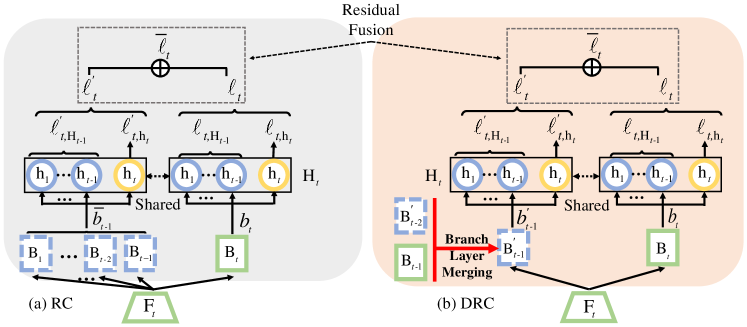
Figure 3: Illustrations of the residual classifier (RC) and the proposed dynamic residual classifier (DRC) for CIL at task $t$. The residual fusion of overall logits, ${{{\rm{\bar{\ell}}}}_{t}}$, is shown. $\operatorname{F}_{t}$ is the backbone feature extractor.

3 Methodology

In class incremental learning, a model is learned from a sequence of ${T}$ tasks, where the task ${t}$ has a set of $n_{t}$ different classes ${C_{t}}=\{c_{t,1},c_{t,2},\cdots,c_{t,n_{t}}\}$. The classes in different tasks are disjoint, ${C_{i}}\cap{C_{j}}=\emptyset,\forall i,j\in\{1,...,T\}$. The training data of task $t$ denotes as ${D_{t}}$. It contains data tuples in the form of $(x,y)$ where $x$ is the image and $y$ is its ground-truth class label. When training on task ${t}$, the model can only access to ${D_{t}}$. With rehearsal applied, data samples from previous tasks are maintained in a memory buffer $M_{t}$ with a relatively small size, i.e., $|{M_{t}}|\ll|{D_{t}}|$. $M_{t}$ is also included in the learning procedure of task $t$. Updates of the memory buffer are dynamic when the task increment proceeds, as shown in Fig. 1. During testing, data samples are from all observed classes so far with balanced distributions.

3.1 Residual Classifier for CIL

The residual classifier (RC) [7] is with the branch layer architecture and residual fusion mechanism. RC can be used to handle the dynamic data imbalance of CIL. Specifically, the classification model $\Phi_{t}$ with RC consists of three parts, the feature extractor $\operatorname{F}_{t}$, the branch layers ${\operatorname{B}_{1},\cdots,\operatorname{B}_{t}}$ and the classifier heads $\operatorname{H}_{t}=\{{\operatorname{h}_{1}},{\operatorname{h}_{2}},\cdots,{\operatorname{h}_{t}}\}$, as illustrated in Fig. 3(a). The feature representation of an input image $x$ is

$$f=\operatorname{F}_{t}(x),$$ (1)

where $f\in\mathbb{R}^{d}$ and $\operatorname{F}_{t}$ is parameterized with $\theta_{t}$. The branch layers are task-specific under the CIL setting. $\operatorname{B}_{1},\cdots,\operatorname{B}_{t-1}$ are inherited from the previous model $\Phi_{t-1}$ to preserve the old knowledge. Therefore, they are frozen at the new task $t$. $\operatorname{B}_{t}$ is for task $t$ and learned with other parts of $\Phi_{t}$. All branches are lightweight, i.e., the $1\times 1$ convolutional layers without bias terms, to alleviate the growing overhead of model parameters. The output of the branch layer $\operatorname{B}_{i}$ is

$$b_{i}=\operatorname{B}_{i}(f)=\omega_{\operatorname{B}_{i}}\cdot f,$$ (2)

where $\omega_{\operatorname{B}_{i}}$ is the weight of branch layer and $\cdot$ is matrix multiplication, $i=1,\cdots,t$. To encode the knowledge of all previous tasks, their outputs are averaged,

$$\bar{b}_{t-1}=\frac{b_{1}+\cdots+b_{t-1}}{t-1},$$ (3)

with $t\geq 2$. $\operatorname{H}_{t}$ is a set of task-specific classifiers ${{\operatorname{h}_{1}},{\operatorname{h}_{2}},\cdots,{\operatorname{h}_{t}}}$, where $\operatorname{h}_{i}$ corresponds to the classifier of task $i,i=1,\cdots,t$. $\operatorname{h}_{i}$ is an FC layer with output dimension $|C_{i}|$. Different logits of classifiers are computed via

$$\left\{{\begin{array}[]{*{20}{l}}\ell^{{}^{\prime}}_{t,\operatorname{H}_{t-1}}=\operatorname{H}_{t-1}(\bar{b}_{t-1}),\\ \ell^{{}^{\prime}}_{t,h_{t}}=h_{t}(\bar{b}_{t-1}),\\ \ell_{t,\operatorname{H}_{t-1}}=\operatorname{H}_{t-1}(b_{t}),\\ \ell_{t,h_{t}}=h_{t}(b_{t}),\end{array}}\right.$$ (4)

as depicted in Fig. 3(a). $\ell_{t}$ and $\ell^{{}^{\prime}}_{t}$ are the overall logits of two branches respectively. Taking $\ell_{t}$ as an example, its computation is

$$\ell_{t}=\operatorname{H}_{t}(b_{t})=[\operatorname{H}_{t-1}(b_{t}),\ell_{t,h_{t}}]=[\ell_{t,\operatorname{H}_{t-1}},\ell_{t,h_{t}}]$$ (5)

where $[\cdot]$ is the concatenate operation and $\ell_{t}\in\mathbb{R}^{|C_{1}|+\cdots+|C_{t}|}$ covers all classes seen so far. The probabilistic output of $\ell_{t}$ is $p_{t}=\operatorname{Softmax}(\ell_{t})$. $\ell^{{}^{\prime}}_{t}$ can be obtained in the similar way with $\bar{b}_{t-1}$ as input.

The residual fusion is applied to the corresponding logits between the two branches. Three fused logits are computed via

$$\left\{{\begin{array}[]{*{20}{l}}{{{{\rm{\bar{\ell}}}}_{t}}=\frac{1}{2}({\ell_{t}}+\ell_{t}^{{}^{\prime}})},\\ {{{{\rm{\bar{\ell}}}}_{t,{\operatorname{H}_{t-1}}}}=\frac{1}{2}({\ell_{t,{\operatorname{H}_{t-1}}}}+\ell_{t,{\operatorname{H}_{t-1}}}^{{}^{\prime}})},\\ {{{{\rm{\bar{\ell}}}}_{t,{\operatorname{h}_{t}}}}=\frac{1}{2}({\ell_{t,{\operatorname{h}_{t}}}}+\ell_{t,{\operatorname{h}_{t}}}^{{}^{\prime}})}.\end{array}}\right.$$ (6)

$\bar{\ell}_{t}$ is the fused logits of all categories till task $t$. $\bar{\ell}_{t,\operatorname{H}_{t-1}}$ fuses the logits of old tasks. $\bar{\ell}_{t,\operatorname{h}_{t}}$ is the logits for new categories at task $t$.

3.2 Dynamic Residual Classifier

The residual classifier (RC) still suffers from the growing storage and computation overhead as more task-specific branch layers are introduced under the CIL setting. Dynamic Residual Classifier is proposed to handle this issue via the branch layer merging in an iterative manner. Assuming the task increment proceeds from $t-1$ to $t$, $\operatorname{B}^{{}^{\prime}}_{t-2}$ and $\operatorname{B}_{t-1}$ are the two branch layers inherited from task $t-1$. As the branch layers are instantiated with the lightweight $1\times 1$ convolutional layer without bias term, $\operatorname{B}^{{}^{\prime}}_{t-2}$ and $\operatorname{B}_{t-1}$ are parameterized by the weight matrices $\omega_{\operatorname{B}^{{}^{\prime}}_{t-2}}$ and $\omega_{\operatorname{B}_{t-1}}$ respectively. A new branch layer $\operatorname{B}^{{}^{\prime}}_{t-1}$ is obtained by merging $\operatorname{B}^{{}^{\prime}}_{t-2}$ and $\operatorname{B}_{t-1}$ in the parameter space,

$${\omega_{\operatorname{B}_{t-1}^{{}^{\prime}}}}=\frac{{\omega_{{\operatorname{B}_{t-1}}}}+{\omega_{\operatorname{B}_{t-2}^{{}^{\prime}}}}}{2}.$$ (7)

$\operatorname{B}^{{}^{\prime}}_{t-1}$ is frozen to preserve the discriminative knowledge learned from previous tasks, as shown in Fig. 3(b). The model-growing problem in RC is thus handled by DRC with only two branch layers, $\operatorname{B}^{{}^{\prime}}_{t-1}$ and $\operatorname{B}_{t}$, included for each task. Moreover, it is interesting to show that the final logit $\bar{\ell}_{t-1}$ of the previous model $\Phi_{t-1}$ is consistent with the output logit $\ell^{{}^{\prime}}_{t,\operatorname{H}_{t-1}}$ of branch $\operatorname{B}^{{}^{\prime}}_{t-1}$ at task $t$,

$$\begin{array}[]{l}\bar{\ell}_{t-1}=\frac{1}{2}({\operatorname{H}_{t-1}}({\operatorname{B}_{t-1}}(f))+{\operatorname{H}_{t-1}}(\operatorname{B}_{t-2}^{{}^{\prime}}(f)))\\ =\frac{1}{2}({\operatorname{H}_{t-1}}({\omega_{{\operatorname{B}_{t-1}}}}\cdot f)+{\operatorname{H}_{t-1}}({\omega_{\operatorname{B}_{t-2}^{{}^{\prime}}}}\cdot f))\\ ={\omega_{{\operatorname{H}_{t-1}}}}\cdot(\frac{1}{2}({\omega_{{\operatorname{B}_{t-1}}}}+{\omega_{\operatorname{B}_{t-2}^{{}^{\prime}}}})\cdot f)+{{\kappa_{{\operatorname{H}_{t-1}}}}}\\ ={\omega_{{\operatorname{H}_{t-1}}}}\cdot({\omega_{\operatorname{B}_{t-1}^{{}^{\prime}}}}\cdot f)+{{\kappa}_{{\operatorname{H}_{t-1}}}}\\ ={\operatorname{H}_{t-1}}(\operatorname{B}_{t-1}^{{{}^{\prime}}}(f))\\ =\ell^{{}^{\prime}}_{t,\operatorname{H}_{t-1}},\end{array}$$ (8)

where ${\omega_{{\operatorname{H}_{t-1}}}}$ and ${{\kappa_{{\operatorname{H}_{t-1}}}}}$ are the weight and bias of the classifier ${\operatorname{H}_{t-1}}$ respectively. The effectiveness of simple branch layer merging can be further demonstrated by this observation. The output logits of the DRC are also computed with the residual fusion mechanism as in Eq. 6.

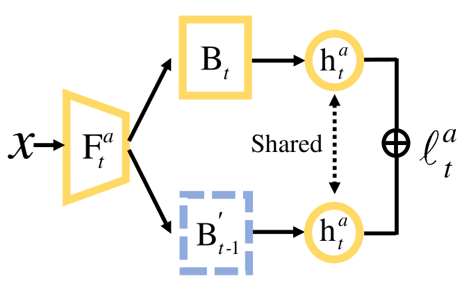
Figure 4: Model $\Phi_{t}^{a}$ with DRC for Adaptation.

3.3 CIL Pipelines with DRC

The combinations between DRC and three CIL pipelines, the model adaptation and fusion (MAF), the model direct transfer (MDT), and the model expansion and compression (MEC), are presented. The resulting methods, MAFDRC, MDTDRC, and MECDRC, are also compared.

MAFDRC  The MAF pipeline consists of two successive stages, the model adaptation and then fusion, as shown in Fig. 2(c). In the adaptation stage, a trainable model $\Phi^{a}_{t}$ with DRC is depicted as in Fig. 4. Specifically, $\operatorname{B}_{t-1}^{{}^{\prime}}$ is obtained via the branch layer merging as Eq. 7 and fixed. $\ell_{t}^{a}$ is the residual fusion between the output logits of the two branches. With cross-entropy as the learning objective,

$$\mathcal{L}_{c}^{a}=\sum\limits_{(x,y)\in{D_{t}}}{\operatorname{CE}(\ell_{t}^{a},y)},$$ (9)

$\Phi_{t}^{a}$ is end-to-end optimized on current task $t$ with $D_{t}$ only.

In the model fusion stage, our aim is to integrate the knowledge from different models, i.e., $\Phi_{t-1}$ and $\Phi_{t}^{a}$, into a single $\Phi_{t}$ while reducing the impact of data imbalance. $\Phi_{t}$ is instantiated with the model architecture as in Fig. 3(b). $\operatorname{B}_{t-1}^{{}^{\prime}}$ is from the branch layer merging and $\operatorname{B}_{t}$ is initialized with the corresponding branch of $\Phi_{t}^{a}$. The classification loss $\mathcal{L}_{c}^{branch}$ consists of two terms,

$$\mathcal{L}_{c}^{branch}=\sum\limits_{(x,y)\in{D_{t}}\cup{M_{t}}}{\operatorname{CE}(\ell_{t},y)}+\sum\limits_{(x,y)\in{M_{t}}}{\operatorname{CE}(\ell_{t,\operatorname{H}_{t-1}}^{{}^{\prime}},y)}.$$ (10)

They guide the learning of the two branches and encourage parameter specialization for old and new classes respectively. ${L_{c}^{fusion}}$ is proposed to optimize the model over all the classes across tasks, with the fused logit $\bar{\ell}_{t}$ from Eq. 6,

$$\begin{split}{\mathcal{L}_{c}^{fusion}}=\sum\limits_{(x,y)\in{D_{t}}\cup{M_{t}}}{\operatorname{CE}(\bar{\ell}_{t},y)}.\end{split}$$ (11)

Moreover, the discriminative knowledge from $\Phi_{t}^{a}$ and $\Phi_{t-1}$ are distilled into the final model $\Phi_{t}$ with the loss,

$$\begin{split}\mathcal{L}_{distil}=\sum\limits_{(x,y)\in{D_{t}}\cup{M_{t}}}\operatorname{KL}(p_{t-1}||\bar{p}_{t,\operatorname{H}_{t-1}})+\operatorname{KL}(p_{t}^{a}||\bar{p}_{t,\operatorname{h}_{t}}),\end{split}$$ (12)

where $\bar{p}_{t,\operatorname{H}_{t-1}}$ can be represented by $\operatorname{S}(\bar{\ell}_{t,\operatorname{H}_{t-1}})$, and $\bar{p}_{t,\operatorname{h}_{t}}$ can be represented by $\operatorname{S}(\bar{\ell}_{t,\operatorname{h}_{t}})$). In the model fusion step, $\Phi_{t}$ is optimized on the overall loss,

$${\mathcal{L}_{all}}=(1-\alpha){\mathcal{L}_{c}^{fusion}}+\alpha{\mathcal{L}_{c}^{branch}+\beta{\mathcal{L}_{distil}}},$$ (13)

with balancing hyper-parameters $0\leq\alpha\leq 1$ and $\beta$.

MDTDRC  In the MDT pipeline, distillation loss is used to directly transfer the knowledge of the previous task from $\Phi_{t-1}$ (the teacher) to $\Phi_{t}$ (the student) and prevent the representations of previous data from drifting too much during new task learning, as illustrated in Fig. 2(a). The proposed DRC is enabled by introducing the branch layers, $\operatorname{B}_{t}$ and $\operatorname{B}_{t-1}^{{}^{\prime}}$. The parameters of $\operatorname{B}_{t-1}^{{}^{\prime}}$ are obtained via Eq. 7 and $\operatorname{B}_{t}$ for the new task is random initialized.

MECDRC  In the model expansion stage, the previous model is frozen and expanded with a new trainable one by concatenating their feature representations. The resulting larger model is then trained with $D_{t}$ and $M_{t}$, as shown in Fig. 2(b). The proposed DRC is also introduced at this stage to boost the performance of the large model across tasks. In the mode compression stage, the expanded model is distilled into the final model with a smaller size.

Comparisons among Three Pipelines  MDT usually impose a challenge to find the balance between learning novel classes and preserving old knowledge simultaneously within a single model. Model expansion can achieve better balance at the price of storage and computation overhead, while model compression may neutralize the improvements from expansion. In MAF, $\Phi_{t}^{a}$ is optimized with only new data $D_{t}$ in the first stage. $\Phi_{t-1}$ preserves the knowledge of previous tasks. The complementary knowledge in $\Phi_{t}^{a}$ and $\Phi_{t-1}$ is then fused into $\Phi_{t}$ by distillation to improve performance on both old and new tasks. Moreover, DRC is integrated into both stages of MAF rather than a single stage of MEC or MDT. To this end, MAFDRC is chosen as our main method.

4 Experiments

Methods	ImageNet100 B0						ImageNet100 B50				ImageNet1000
	5 steps		10 steps		20 steps		5 steps		10 steps		10 steps
	Avg	Last	Avg	Last	Avg	Last	Avg	Last	Avg	Last	Avg	Last
iCaRL [37]	74.87	63.36	70.35	55.78	67.80	51.78	64.69	54.46	57.92	50.52	54.15	36.25
BiC [43]	77.11	67.10	70.98	52.00	63.79	41.70	68.51	54.36	60.73	43.04	61.66	41.30
WA [49]	77.59	68.36	73.59	60.78	68.81	57.16	68.49	59.74	62.10	54.42	59.23	40.92
PODNet [15]	76.73	64.90	70.13	53.30	62.78	47.10	78.41	69.18	75.97	66.50	-	-
DER w/o p [44]	81.03	74.44	78.30	70.40	78.22	71.40	80.30	74.28	78.58	71.66	67.41	58.56
FOSTER B4 [42]	79.59	72.58	76.54	67.08	74.21	62.16	79.93	72.48	76.27	67.04	68.34	58.53
FOSTER [42]	78.38	71.38	76.22	66.70	73.95	62.42	79.56	71.18	75.79	66.90	-	-
MAFDRC	82.22	76.01	79.66	70.41	75.21	63.59	81.37	74.86	77.95	71.26	69.37	59.59

Table 1: Results on ImageNet100 B0, B50 and ImageNet1000 B0 settings. DER w/o P means DER without pruning. FOSTER B4 means the model before feature compression.

(a) ImageNet100 B0 10 steps

(b) ImageNet100 B50 10 steps

(c) ImageNet1000 B0 10 steps

Figure 5: Incremental Accuracy on ImageNet. The top-1 accuracy (%) after learning each task is shown.

4.1 Experimental Setup and Details

Datasets  ImageNet1000 [11] is a large-scale dataset with 1,000 classes that includes 1.28 million images for training and 50,000 images for validation. ImageNet100 [11] is made up of 100 randomly selected classes from ImageNet1000. CIFAR100 [31] consists of 100 classes and each class has 600 images, of which 500 are used as the training set and 100 are used as the test set.

Protocols  For ImageNet100 and CIFAR100, we validate the proposed method in two widely used CIL protocols: (1) B0 (base 0) [37]: In this protocol, a model is gradually trained on 5 steps (20 new classes per step), 10 steps (10 new classes per step) and 20 steps (5 new classes per step) with the fixed memory size of 2,000 exemplars. (2) B50 (base 50) [25]: A model is trained first on 50 classes. The remaining 50 classes are used for continual learning with 5, 10 classes per step. The memory size is fixed to 20 exemplars per class. For ImageNet1000, we evaluate our method on the protocol [37] where a model is trained on all 1,000 classes with 100 classes per step (10 steps in total). The fixed memory size is 20,000 exemplars. We also carried out the LT-CIL experiments on CIFAR100 and ImageNet100 following the protocol [33]. Two classification accuracy are reported. ”Avg” is the average accuracy over incremental steps. ”Last” is the accuracy of the last step.

Implementation Details  Our method is implemented with PyTorch [20] and PyCIL [50]. The standard 18-layer ResNet [22] is used as the backbone feature extractor for ImageNet. For CIFAR100, a modified 32-layer ResNet [37] is used instead. In our experiments, the MDT setting follows [37], that of MEC is from [42], and the MAF one is based on [24] in all experiments. Integrating the proposed DRC with the MAF pipeline results in our main method, MAFDRC. For different CIL settings, similar optimization is used. In model adaptation, the SGD optimizer with a momentum of 0.9 is used for training 70 epochs in total. The initial learning rate is set to 0.1 and gradually reduces to zero with a cosine annealing scheduler. In model fusion, the above settings are followed, but training 130 epochs in total. For data augmentation, we follow the practice in FOSTER [42], where the AutoAugment [6] is used along with the common random cropping and horizontal flip. For a fair comparison, the reported CIL results of all competitors in this work are reproduced with such an augmentation. In the LT-CIL scenario, our experimental setting is exactly the same as in [33]. The balancing hyperparameters ${\alpha}$ and $\beta$ in Eq. 13 are set to 0.2 and 4 respectively via cross-validation.

Methods	CIFAR100 B0						CIFAR100 B50
	5 steps		10 steps		20 steps		5 steps		10 steps
	Avg	Last	Avg	Last	Avg	Last	Avg	Last	Avg	Last
iCaRL  [37]	69.29	57.03	68.37	53.04	67.43	49.65	62.21	53.63	53.65	47.18
BiC  [43]	68.66	58.22	67.75	53.31	65.41	47.12	63.92	54.18	59.68	48.04
WA  [49]	72.09	61.49	70.88	56.74	68.10	49.60	67.30	59.37	61.86	50.86
PODNet  [15]	69.32	57.75	63.17	47.49	58.26	40.62	70.40	62.49	69.20	60.14
DER w/o P  [44]	75.83	68.95	75.71	65.85	74.04	62.53	72.95	68.06	72.50	67.37
FOSTER B4  [42]	74.53	65.31	73.13	61.81	70.64	56.84	71.31	64.66	68.90	61.41
FOSTER  [42]	72.46	63.35	71.80	60.15	69.56	56.50	70.09	63.63	68.05	60.71
MAFDRC	74.87	66.45	73.97	62.04	71.75	57.65	71.65	65.09	70.21	62.20

Table 2: Results on CIFAR100 B0, B50 setting.

(a) B0 10 steps

(b) B0 20 steps

(c) B50 10 steps

Figure 6: Incremental Accuracy on CIFAR100. The top-1 accuracy (%) after learning each task is shown.

		CIFAR100		ImageNet100
Methods		5 steps	10 steps	5 steps	10 steps
	EEIL	38.46	37.50	50.68	50.63
	+Two Stage[33]	38.97	37.58	51.36	50.74
	LUCIR	42.69	42.15	52.91	52.80
	+Two Stage[33]	45.88	45.73	54.22	55.41
	PODNet	44.07	43.96	58.78	58.94
	+Two Stage[33]	44.38	44.35	58.82	59.09
	MAF	35.92	33.70	46.62	35.83
Ordered LT-CIL	MAFDRC	53.13	49.01	60.69	59.65
	EEIL	31.91	32.44	42.87	43.72
	+Two Stage[33]	34.19	33.70	49.31	48.26
	LUCIR	35.09	34.59	45.80	46.52
	+Two Stage[33]	39.40	39.00	52.08	51.91
	PODNet	34.64	34.84	49.69	51.05
	+Two Stage[33]	36.37	37.03	51.55	52.60
	MAF	31.63	30.18	41.53	39.92
Shuffled LT-CIL	MAFDRC	41.41	41.84	52.49	56.35

Table 3: LT-CIL [33] results with average accuracy reported.

4.2 Main Results

The results of different CIL methods on both the ImageNet100 and ImageNet1000 are shown in Tab. 1. The proposed MAFDRC achieves the same level of performance as the strong competitors, i.e., FOSTER [42] and DER [44], and becomes one of the state-of-the-art (SOTA) methods. Our method consistently surpasses the FOSTER and its uncompressed variant, FOSTER B4, with clear margins. For example, MAFDRC is better than FOSTER B4 with $3.12\%$ and $1.68\%$ improvements in the averaged accuracy under the B0 10 steps and the B50 10 steps of ImageNet100, respectively. On the large-scale ImageNet1000, such improvement is still more than $1\%$. Similar results are obtained by MAFDRC and the DER w/o P (DER without pruning). Note that DER w/o P is a strong CIL method that keeps expanding its feature extractors and ends up with a much larger model size than ours with the fixed numbers of parameters and feature dimensions across tasks. However, MAFDRC still achieves better results than DER w/o P in multiple settings, including the challenging ImangeNet1000, with nontrivial improvement (usually more than $1\%$). Detailed comparisons among different methods along the incremental learning procedure are illustrated in Fig. 5.

The CIL results on CIFAR100 are shown in Tab. 2 and Fig. 6. DER achieves the best performance at the price of a much larger model size than the proposed method, i.e., the model parameters in DER are rough $k$ times of those in MAFDRC under $k$ steps. Our method achieves the second-best results and is better than other SOTA methods with similar model sizes, e.g., FOSTER.

The proposed method is also validated on a new CIL setting, LT-CIL [33], with other SOTA results reported in Tab. 3. Our MAFDRC consistently achieves the new SOTA results on both datasets and settings. More importantly, the proposed method boosts its baseline, the MAF pipeline, with more than $10\%$ in most cases. It suggests the effectiveness of the proposed dynamic residual classifier (DRC) in handling the data imbalance issue.

4.3 Detailed Analysis

The results of CIFAR100 B0 10 steps and ImageNet100 B0 10 steps are reported by default. More results can be found in the Supplementary Material.

Components			CIFAR100		ImageNet100
MAF	DRC	LA	Avg	Last	Avg	Last
			65.59	50.56	68.95	54.18
✓			69.61	54.84	72.01	58.76
✓	✓		72.80	60.92	78.65	69.88
✓	✓	✓	73.97	62.04	79.66	70.41

Table 4: Contributions of different components in MAFDRC.

Methods	CIFAR100		ImageNet100
	Avg	Last	Avg	Last
MAF	69.61	54.84	72.01	58.76
MAFRC	74.07	61.91	79.26	70.54
MAFDRC	73.97	62.04	79.66	70.41

Table 5: The results of MAF with residual classifier (RC) and dynamic residual classifier (DRC).

Contributions of different components  The results are shown in Tab. 4. The MAF pipeline achieves clearly better results than the finetuning baseline since such a pipeline is a CIL method itself, as discussed in Sec. 2. The proposed DRC brings substantial improvements. For example, DRC enhances MAF results with $6.64\%$ average accuracy and $11.12\%$ last accuracy on ImageNet100. By replacing the conventional classification loss with the adjusted loss, logit adjustment (LA) [36], provides positive effects and results in the proposed method, MAFDRC.

Branch Layer Merging  As shown in Tab. 5, MAFRC clearly improves the baseline. Therefore, the effectiveness of the branch layer architecture and residual fusion mechanism in RC is demonstrated. However, with the increasing task-specific branch layers, MAFRC suffers from the problem of growing model size. DRC handles this issue with branch layer merging, resulting in a more efficient model, MAFDRC. Moreover, MAFDRC is as effective as MAFRC, as suggested by their performance in Tab. 5.

Model	CIFAR100		ImageNet100
	Avg	Last	Avg	Last
MAF	69.61	54.84	72.01	58.76
+DRC	72.80 ($\uparrow$3.19)	60.92 ($\uparrow$6.08)	78.65 ($\uparrow$6.64)	69.88 ($\uparrow$11.12)
MEC	69.02	52.86	70.08	55.06
+DRC	70.25 ($\uparrow$1.23)	54.76 ($\uparrow$1.90)	71.41 ($\uparrow$1.33)	58.54 ($\uparrow$3.48)
MDT	67.69	52.56	69.40	54.68
+DRC	70.80 ($\uparrow$3.11)	58.28 ($\uparrow$5.72)	71.31 ($\uparrow$1.91)	59.34 ($\uparrow$4.66)

Table 6: The results of different pipelines with DRC.

CIL Pipelines with DRC  As shown in Tab. 6, DRC is compatible with all three pipelines and clearly boosts their performance. MAF benefits the most.

Methods	CIFAR100		ImageNet100
	Avg	Last	Avg	Last
MAF	69.61	54.84	72.01	58.76
MAF+BFT [28]	69.75	55.19	73.08	59.96
MAF+WA [49]	70.14	56.23	73.94	62.14
MAF+DRC	72.80	60.92	78.65	69.88

Table 7: The results of different imbalanced methods.

Data Imbalanced Methods  The balanced fine-tuning (BFT) [28] and the weight aligning (WA) [49] are alternatives to DRC for handling the data imbalance in CIL. As shown in Tab. 7, both BFT and WA bring some improvements to the MAF pipeline but are inferior to our DRC.

Hyper-parameters  The memory size of the B0 protocol [37] is reduced to 20 exemplars per class. The results are reported in Tab. 8. Our MAFDRC still achieves the SOTA level performance. The performance of our methods with different hyper-parameter values of Eq. 13 are shown in Fig. 7. Our method is not sensitive to such changes.

Methods	CIFAR100		ImageNet100
	Avg	Last	Avg	Last
DER w/o P	71.99	62.66	76.49	69.42
FOSTER B4	71.16	59.40	75.63	64.90
FOSTER	69.79	58.33	74.58	64.72
MAFDRC	71.24	59.73	77.88	69.64

Table 8: CIL results with reserving 20 exemplars per class.

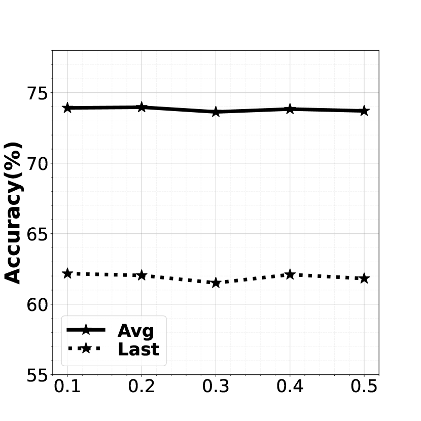
(a) $\alpha$

(b) $\beta$

Figure 7: Impacts of $\alpha$s and $\beta$s. CIFAR100 B0 10 steps is used.

5 Conclusion

In this paper, the dynamic nature of the data imbalance in the widely used CIL rehearsal strategy is shown. We aim to handle this challenging scenario with a novel dynamic residual classifier (DRC). This is complementary to the adjusted losses and data re-samplings used by many CIL methods based on the static viewpoint. The proposed DRC adopts the branch layer architecture and the residual fusion mechanism of a recent advance residual classifier (RC) and handles the model-growing problem with the branch layer merging. As a generalizable method, DRC substantially improves the performance of different CIL pipelines and achieves SOTA performance under both the CIL and LT-CIL settings.

Acknowledgement  This research is supported partly by the National Science Foundation for Young Scientists of China (No. 62106289), partly by National Natural Science Foundation of China (No. 62232008), partly by Guangdong HUST Industrial Technology Research Institute, Guangdong Provincial Key Laboratory of Manufacturing Equipment Digitization (2020B1212060014).

References

- [1] Mateusz Buda, Atsuto Maki, and Maciej A Mazurowski. A systematic study of the class imbalance problem in convolutional neural networks. Neural Networks, 2018.
- [2] Jonathon Byrd and Zachary Lipton. What is the effect of importance weighting in deep learning? In International Conference on Machine Learning (ICML), 2019.
- [3] Francisco M Castro, Manuel J Marín-Jiménez, Nicolás Guil, Cordelia Schmid, and Karteek Alahari. End-to-end incremental learning. In Proceedings of the European Conference on Computer Vision (ECCV), 2018.
- [4] Arslan Chaudhry, Puneet K Dokania, Thalaiyasingam Ajanthan, and Philip HS Torr. Riemannian walk for incremental learning: Understanding forgetting and intransigence. In Proceedings of the European Conference on Computer Vision (ECCV), 2018.
- [5] Yoojin Choi, Mostafa El-Khamy, and Jungwon Lee. Dual-teacher class-incremental learning with data-free generative replay. In Proceedings of the IEEE Conference on Computer Vision and Pattern Recognition (CVPR), 2021.
- [6] Ekin D Cubuk, Barret Zoph, Dandelion Mane, Vijay Vasudevan, and Quoc V Le. Autoaugment: Learning augmentation strategies from data. In Proceedings of the IEEE Conference on Computer Vision and Pattern Recognition (CVPR), 2019.
- [7] Jiequan Cui, Shu Liu, Zhuotao Tian, Zhisheng Zhong, and Jiaya Jia. Reslt: Residual learning for long-tailed recognition. IEEE Transactions on Pattern Analysis and Machine Intelligence (TPAMI), 2022.
- [8] Yin Cui, Menglin Jia, Tsung-Yi Lin, Yang Song, and Serge Belongie. Class-balanced loss based on effective number of samples. In Proceedings of the IEEE Conference on Computer Vision and Pattern Recognition (CVPR), 2019.
- [9] Matthias De Lange, Rahaf Aljundi, Marc Masana, Sarah Parisot, Xu Jia, Aleš Leonardis, Gregory Slabaugh, and Tinne Tuytelaars. A continual learning survey: Defying forgetting in classification tasks. IEEE Transactions on Pattern Analysis and Machine Intelligence (TPAMI), 2021.
- [10] Matthias De Lange, Rahaf Aljundi, Marc Masana, Sarah Parisot, Xu Jia, Aleš Leonardis, Gregory Slabaugh, and Tinne Tuytelaars. A continual learning survey: Defying forgetting in classification tasks. IEEE Transactions on Pattern Analysis and Machine Intelligence (TPAMI), 2021.
- [11] Jia Deng, Wei Dong, Richard Socher, Li-Jia Li, Kai Li, and Li Fei-Fei. Imagenet: A large-scale hierarchical image database. In Proceedings of the IEEE Conference on Computer Vision and Pattern Recognition (CVPR), 2009.
- [12] Debashree Devi, Biswajit Purkayastha, et al. Redundancy-driven modified tomek-link based undersampling: A solution to class imbalance. Pattern Recognition Letters, 2017.
- [13] Prithviraj Dhar, Rajat Vikram Singh, Kuan-Chuan Peng, Ziyan Wu, and Rama Chellappa. Learning without memorizing. In Proceedings of the IEEE Conference on Computer Vision and Pattern Recognition (CVPR), 2019.
- [14] Alexey Dosovitskiy, Lucas Beyer, Alexander Kolesnikov, Dirk Weissenborn, Xiaohua Zhai, Thomas Unterthiner, Mostafa Dehghani, Matthias Minderer, Georg Heigold, Sylvain Gelly, et al. An image is worth 16x16 words: Transformers for image recognition at scale. In Proceedings of the International Conference on Learning Representations (ICLR), 2021.
- [15] Arthur Douillard, Matthieu Cord, Charles Ollion, Thomas Robert, and Eduardo Valle. Podnet: Pooled outputs distillation for small-tasks incremental learning. In Proceedings of the European Conference on Computer Vision (ECCV), 2020.
- [16] Arthur Douillard, Alexandre Ramé, Guillaume Couairon, and Matthieu Cord. Dytox: Transformers for continual learning with dynamic token expansion. In Proceedings of the IEEE Conference on Computer Vision and Pattern Recognition (CVPR), 2022.
- [17] Robert M French. Catastrophic forgetting in connectionist networks. Trends in Cognitive Sciences, 1999.
- [18] Robert M French and Nick Chater. Using noise to compute error surfaces in connectionist networks: A novel means of reducing catastrophic forgetting. Neural Computation, 2002.
- [19] Ian Goodfellow, Jean Pouget-Abadie, Mehdi Mirza, Bing Xu, David Warde-Farley, Sherjil Ozair, Aaron Courville, and Yoshua Bengio. Generative adversarial networks. Communications of the ACM, 2020.
- [20] Stephen T Grossberg. Studies of mind and brain: Neural principles of learning, perception, development, cognition, and motor control. Springer Science & Business Media, 2012.
- [21] Haibo He and Edwardo A Garcia. Learning from imbalanced data. IEEE Transactions on Knowledge and Data Engineering (TKDE), 2009.
- [22] Kaiming He, Xiangyu Zhang, Shaoqing Ren, and Jian Sun. Deep residual learning for image recognition. In Proceedings of the IEEE Conference on Computer Vision and Pattern Recognition (CVPR), 2016.
- [23] Geoffrey Hinton, Oriol Vinyals, Jeff Dean, et al. Distilling the knowledge in a neural network. arXiv preprint arXiv:1503.02531, 2015.
- [24] Saihui Hou, Xinyu Pan, Chen Change Loy, Zilei Wang, and Dahua Lin. Lifelong learning via progressive distillation and retrospection. In Proceedings of the European Conference on Computer Vision (ECCV), 2018.
- [25] Saihui Hou, Xinyu Pan, Chen Change Loy, Zilei Wang, and Dahua Lin. Learning a unified classifier incrementally via rebalancing. In Proceedings of the IEEE Conference on Computer Vision and Pattern Recognition (CVPR), 2019.
- [26] Ching-Yi Hung, Cheng-Hao Tu, Cheng-En Wu, Chien-Hung Chen, Yi-Ming Chan, and Chu-Song Chen. Compacting, picking and growing for unforgetting continual learning. In Advances in Neural Information Processing Systems (NeurIPS), 2019.
- [27] David Isele and Akansel Cosgun. Selective experience replay for lifelong learning. In Proceedings of the AAAI Conference on Artificial Intelligence (AAAI), 2018.
- [28] Bingyi Kang, Saining Xie, Marcus Rohrbach, Zhicheng Yan, Albert Gordo, Jiashi Feng, and Yannis Kalantidis. Decoupling representation and classifier for long-tailed recognition. In Proceedings of the International Conference on Learning Representations (ICLR), 2020.
- [29] Harsurinder Kaur, Husanbir Singh Pannu, and Avleen Kaur Malhi. A systematic review on imbalanced data challenges in machine learning: Applications and solutions. ACM Computing Surveys (CSUR), 2019.
- [30] Jong-Yeong Kim and Dong-Wan Choi. Split-and-bridge: Adaptable class incremental learning within a single neural network. In Proceedings of the AAAI Conference on Artificial Intelligence (AAAI), 2021.
- [31] Alex Krizhevsky, Geoffrey Hinton, et al. Learning multiple layers of features from tiny images. Technical Report TR-2009, University of Toronto, Toronto, 2009.
- [32] Xilai Li, Yingbo Zhou, Tianfu Wu, Richard Socher, and Caiming Xiong. Learn to grow: A continual structure learning framework for overcoming catastrophic forgetting. In International Conference on Machine Learning (ICML), 2019.
- [33] Xialei Liu, Yu-Song Hu, Xu-Sheng Cao, Andrew D Bagdanov, Ke Li, and Ming-Ming Cheng. Long-tailed class incremental learning. In Proceedings of the European Conference on Computer Vision (ECCV), 2022.
- [34] David Lopez-Paz and Marc’Aurelio Ranzato. Gradient episodic memory for continual learning. In Advances in Neural Information Processing Systems (NeurIPS), 2017.
- [35] Marc Masana, Xialei Liu, Bartlomiej Twardowski, Mikel Menta, Andrew D Bagdanov, and Joost van de Weijer. Class-incremental learning: survey and performance evaluation on image classification. IEEE Transactions on Pattern Analysis and Machine Intelligence (TPAMI), 2022.
- [36] Aditya Krishna Menon, Sadeep Jayasumana, Ankit Singh Rawat, Himanshu Jain, Andreas Veit, and Sanjiv Kumar. Long-tail learning via logit adjustment. In Proceedings of the International Conference on Learning Representations (ICLR), 2021.
- [37] Sylvestre-Alvise Rebuffi, Alexander Kolesnikov, Georg Sperl, and Christoph H Lampert. icarl: Incremental classifier and representation learning. In Proceedings of the IEEE Conference on Computer Vision and Pattern Recognition (CVPR), 2017.
- [38] David Rolnick, Arun Ahuja, Jonathan Schwarz, Timothy Lillicrap, and Gregory Wayne. Experience replay for continual learning. In Advances in Neural Information Processing Systems (NeurIPS), 2019.
- [39] Joan Serra, Didac Suris, Marius Miron, and Alexandros Karatzoglou. Overcoming catastrophic forgetting with hard attention to the task. In International Conference on Machine Learning (ICML), 2018.
- [40] Hanul Shin, Jung Kwon Lee, Jaehong Kim, and Jiwon Kim. Continual learning with deep generative replay. In Advances in Neural Information Processing Systems (NeurIPS), 2017.
- [41] Gido M Van de Ven and Andreas S Tolias. Three scenarios for continual learning. In Advances in Neural Information Processing Systems (NeurIPS) Workshop, 2019.
- [42] Fu-Yun Wang, Da-Wei Zhou, Han-Jia Ye, and De-Chuan Zhan. Foster: Feature boosting and compression for class-incremental learning. In Proceedings of the European Conference on Computer Vision (ECCV), 2022.
- [43] Yue Wu, Yinpeng Chen, Lijuan Wang, Yuancheng Ye, Zicheng Liu, Yandong Guo, and Yun Fu. Large scale incremental learning. In Proceedings of the IEEE Conference on Computer Vision and Pattern Recognition (CVPR), 2019.
- [44] Shipeng Yan, Jiangwei Xie, and Xuming He. Der: Dynamically expandable representation for class incremental learning. In Proceedings of the IEEE Conference on Computer Vision and Pattern Recognition (CVPR), 2021.
- [45] Lu Yang, He Jiang, Qing Song, and Jun Guo. A survey on long-tailed visual recognition. International Journal of Computer Vision (IJCV), 2022.
- [46] Xiao Zhang, Zhiyuan Fang, Yandong Wen, Zhifeng Li, and Yu Qiao. Range loss for deep face recognition with long-tailed training data. In Proceedings of the IEEE Conference on Computer Vision and Pattern Recognition (CVPR), 2017.
- [47] Yifan Zhang, Bingyi Kang, Bryan Hooi, Shuicheng Yan, and Jiashi Feng. Deep long-tailed learning: A survey. arXiv preprint arXiv:2110.04596, 2021.
- [48] Borui Zhao, Quan Cui, Renjie Song, Yiyu Qiu, and Jiajun Liang. Decoupled knowledge distillation. In Proceedings of the IEEE Conference on Computer Vision and Pattern Recognition (CVPR), 2022.
- [49] Bowen Zhao, Xi Xiao, Guojun Gan, Bin Zhang, and Shu-Tao Xia. Maintaining discrimination and fairness in class incremental learning. In Proceedings of the IEEE Conference on Computer Vision and Pattern Recognition (CVPR), 2020.
- [50] Da-Wei Zhou, Fu-Yun Wang, Han-Jia Ye, and De-Chuan Zhan. Pycil: A python toolbox for class-incremental learning. CoRR, abs/2112.12533, 2021.