Age of Information Diffusion on Social Networks: Optimizing Multi-Stage Seeding Strategies

Abstract.

To promote viral marketing, major social platforms (e.g., Facebook Marketplace and Pinduoduo) repeatedly select and invite different users (as seeds) in online social networks to share fresh information about a product or service with their friends. Thereby, we are motivated to optimize a multi-stage seeding process of viral marketing in social networks and adopt the recent notions of the peak and the average age of information (AoI) to measure the timeliness of promotion information received by network users. Our problem is different from the literature on information diffusion in social networks, which limits to one-time seeding and overlooks AoI dynamics or information replacement over time. As a critical step, we manage to develop closed-form expressions that characterize and trace AoI dynamics over any social network. For the peak AoI problem, we first prove the NP-hardness of our multi-stage seeding problem by a highly non-straightforward reduction from the dominating set problem, and then present a new polynomial-time algorithm that achieves good approximation guarantees (e.g., less than 2 for linear network topology). To minimize the average AoI, we also prove that our problem is NP-hard by properly reducing it from the set cover problem. Benefiting from our two-side bound analysis on the average AoI objective, we build up a new framework for approximation analysis and link our problem to a much simplified sum-distance minimization problem. This intriguing connection inspires us to develop another polynomial-time algorithm that achieves a good approximation guarantee. Additionally, our theoretical results are well corroborated by experiments on a real social network.

1. Introduction

Today, omnipresent online social networks (e.g., Facebook and WeChat) have revolutionized the way that people interact and share information, creating viral marketing opportunities for social commerce platforms (e.g., Facebook Marketplace and Pinduoduo) (Chang et al., 2020). Pinduoduo, for example, promotes its products by selecting and inviting its users to push and share promotion information via their WeChat accounts (Pinduoduo, 2023), and these users are well motivated to share with their friends to earn free products and coupons. As promotion information becomes outdated over time, Pinduoduo periodically selects different users as seeds to update promotions to their friends and friends’ friends in the social network timely. Thereby, we are motivated to optimize a practical multi-stage seeding process of viral marketing to keep promotion information that is received by users in social networks as fresh as possible.

To evaluate information freshness from receivers’ perspectives, age of information (AoI), which is coined in (Kaul et al., 2012), is widely adopted as a standard performance metric in the literature (Tripathi and Modiano, 2022; Yates et al., 2021; Talak et al., 2017; Hsu et al., 2017; Xu and Gautam, 2020). AoI measures the time elapsed since the latest information reached its intended user. In the literature, most AoI works either study broadcasting networks where a base station sends time-sensitive information to its clients (e.g., (Bastopcu and Ulukus, 2019; Hsu et al., 2017; Kadota et al., 2018b; Liu et al., 2021)), or focus on monitoring networks where clients coordinate to transmit their collected information to the base station timely (e.g., (Kadota et al., 2018a; Bedewy et al., 2019; Li et al., 2022)). In the context of broadcasting networks, Hsu et al. (Hsu et al., 2017) proposed an MDP-based scheduling algorithm to minimize the long-run average AoI for noiseless channels, and Kadota et al. (Kadota et al., 2018b) minimized the expected weighted sum AoI of the clients for unreliable channels via transmission scheduling. In the context of monitoring networks, Tripathi et al. (Tripathi et al., 2021) studied a mobile agent’s randomized trajectory to mine the data from ground terminals and optimize average AoI. In (Tripathi and Modiano, 2022), Tripathi et al. further studied the correlation among multiple coupled sources and provided an approximation solution for minimizing the weighted-sum average AoI. Besides average AoI, the peak AoI also emerges as another important measure that quantifies the worst case AoI in a fair manner (Tripathi et al., 2021; Xu and Gautam, 2020). In priority queueing systems where a data source sends updates to a single processor, Xu and Gautam (Xu and Gautam, 2020) derived closed-form expressions of the peak AoI, which further allows for analyzing the effects of specific service strategies. It is clear that prior AoI literature does not study fresh information diffusion in a general social network or optimize any seeding strategies over time.

Our multi-stage seeding problem is also different from the traditional social network literature about information diffusion, which only limits to one-time seeding and overlooks AoI dynamics or information replacement over time. When information diffusion meets social networks, Lu et al. (Lu et al., 2015) proposed heuristic algorithms that achieve good performances in certain scenarios. Ioannidis et al. (Ioannidis et al., 2009) studied the problem of dynamic content dissemination in a complete contact (social) graph among users. Yet our social graph is not restricted to being complete and our model needs to consider the AoI process of each node of the entire time horizon rather than solely the final moment, both making our problem and analysis more difficult. For a more comprehensive understanding of social information diffusion, we refer interested readers to some survey works (Bartal and Jagodnik, 2021; Banerjee et al., 2020). The most related classical problem to ours is the NP-hard social influence maximization (SIM) problem (Kempe et al., 2003), which seeks a subset $S\subseteq V$ of cardinality $k$ at a time to maximize the influence spread function $\sigma(S)$ of the given social graph $G=(V,E)$. The submodularity of the objective function yields an approximation ratio of around $1-\frac{1}{e}$ (Nemhauser et al., 1978; Kempe et al., 2003), where $e$ is the base of natural logarithm. Different from ours, SIM overlooks the dynamic information updates in the network (where new information will replace the outdated one) and considers a one-time seeding strategy only, both of which obviously simplifies the algorithm design and theoretical analysis. The other related works include the $k$-median (Cohen-Addad et al., 2022) and the $k$-center problems (Panigrahy and Vishwanathan, 1998; Lu et al., 2015). For symmetric (Hochbaum and Shmoys, 1985) and asymmetric (Panigrahy and Vishwanathan, 1998) graphs, the $k$-center problem achieves an approximation of a constant and an iterated logarithm of the number of nodes, respectively. Since different sequences of dynamically selected seeds make a huge difference in our AoI problem, all the above approximation algorithms and results turn out to be infeasible for our problem.

Our key novelty and main contributions are summarized below.

• Optimizing the Age of Information Diffusion on Social Networks via Multi-stage Seeding Process. To the best of our knowledge, our work is the first to model and optimize a multi-stage information seeding process on social networks (see Section  2). We practically allow fresh information to replace any outdated information during the network diffusion, and our multi-stage seeding process over any social network topology makes it intricate to trace the network AoI dynamics. By considering two different objectives, i.e., the peak and the average AoI of the network, we study the dynamic optimization problem comprehensively.

• Closed-form Characterization of AoI Tracing and NP-hardness Proofs. As a critical step, we successfully derive closed-form expressions that trace the average and peak AoI objectives of any social network in Section  3, respectively, which is highly non-trivial due to the dynamics in the multi-stage seeding process. By non-trivial reductions from the dominating set and set cover problems, respectively, we prove that both of our problems for peak and average AoI minimization are NP-hard.

• Fast Algorithm for peak AoI minimization with Provable Approximation Guarantee. By focusing on a fine-tuned set of seed candidates along the social graph diameter, we design a new polynomial-time algorithm that guarantees good approximations as compared to the optimum (see Section  4). Particularly, our algorithm is proven to achieve an approximation of less than 2 for linear network topology. For a general network topology, we equivalently reduce it to a special histogram structure and analytically provide a provable approximation guarantee.

• Fast Algorithm for average AoI minimization with Provable Approximation Guarantee. As the average AoI explicitly takes into account every user’s AoI dynamics, it is more involved to optimize. We further provide two-side bound analysis to build up a new framework for average AoI approximation analysis (see Section  5). This enables us to link our problem to a remarkably simplified sum-distance minimization problem and helps design a polynomial-time algorithm that achieves a good approximation guarantee. Section 6 validates our theoretical results via experiments on a realistic social network.

Due to page limits, we move omitted proofs and discussions to the appendix.

2. System Model and Problem Statement

We consider a budget-aware viral marketing platform (e.g., Facebook Marketplace and Pinduoduo) that periodically selects $k$ users as seeds to dynamically diffuse $k$ latest promotion updates over the social network. Figure  1 displays the system configuration.

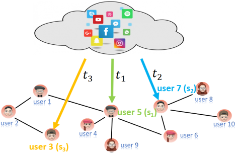
Figure 1. An illustrative example of the viral marketing system where the time gap between two consecutive seeding timestamps is $\Delta=2$. Here, we consider three rounds of seeding as $(s_{1},s_{2},s_{3})=(v_{5},v_{7},v_{3})$ to dynamically choose users 5, 7, 3 at time $t_{1}=1$, $t_{2}=3$ and $t_{3}=5$ for information diffusion.

Formally, we model the social network as an undirected and connected graph $G=(V,E)$, where a node $v\in V$ represents a distinctive user in the network and an edge $(v_{i},v_{j})\in E$ tells a social connection between two users $v_{i}$ and $v_{j}$ to share messages. Suppose the network involves $n$ users and $m$ social connections, i.e., $|V|=n$ and $|E|=m$. We consider discretely slotted time horizon of $T$ slots and index current time by $t\in\{0,1,...,T\}$.

Denote $S_{k}=(s_{1},...,s_{k})$ as the sequence of $k$ seeds that the platform dynamically selects from $V$ to diffuse the latest promotion information within the time horizon. As many viral marketing promotions are practically scheduled in a periodic way (Raja, 2012), we denote the time gap between any two consecutive promotion updates as $\Delta$. That is, at each timestamp $t_{j}=(j-1)\cdot\Delta+1$ with $j\in\{1,...,k\}$, the platform selects a user as seed for viral-marketing.   Table  1 summarizes the key notation of this paper.

Now, we introduce the social information diffusion and AoI models under multi-stage seeding. For any user $v_{i}\in V$ at time $t$, its real-time AoI is denoted as $A(v_{i},t)$ and evolves as follows.

1. When $t=0$, the AoI of each user $v_{i}\in V$ is denoted to be a constant $A_{0}$, i.e., $A(v_{i},0)=A_{0}$. Note that we can easily extend our solution to different initial ages, as shown in Section 6.

2. After a node is selected as the $j$-th seed $s_{j}$ with new source information at timestamp $t_{j}$, the AoI of the node (i.e., seed $s_{j}$) drops to 1 immediately at $t_{j}$, i.e., $A(s_{j},t_{j})=1$ as in (Wang and Duan, 2022; Tripathi and Modiano, 2022).

3. Each seed node will disseminate the new information to its neighbors in the network. Consequently, each neighbor of the seed, after receiving the updated information, will further disseminate the information to her neighbors, and so on and so forth. The information dissemination through each social connection (i.e., edge) consumes a normalized unit of time.

4. At any time, if a node receives multiple information updates from its neighbors, it takes the freshest information and its AoI is reduced to be the smallest age of such updates; otherwise, the AoI of the node will increase linearly over time.

Let us consider an illustrative example of information diffusion and AoI evolution in Figure 1: user 5 is firstly selected as a seed at timestamp $t_{1}=1$, resulting in its AoI to be $A(v_{5},t_{1})=1$ (i.e., user 5’s AoI at time $t_{1}$ is updated to 1). The updated information in green (which is from seed user 5) will reach user 5’s social neighbors (i.e., users 1, 4, 6, 9) after a unit time slot, and the AoI of these neighbor users will be updated to two (which is the age of the green information at time $2$) at time $t_{1}+1=2$. User 5’s social neighbors will further disseminate the information to their neighbors accordingly. Furthermore, when some new information reaches a node, the node will replace its old information with the new one. For instance, at time $t_{1}+2=3$, the green information will reach user 7 by disseminating from user  6. In the meantime of $t_{2}=1+\Delta=3$, user  7 is selected as a new seed to disseminate the new information in blue. Consequently, user  7 will replace its green information with the blue one, yielding $A(v_{7},t_{2})=1$.

Given our practical multi-stage seeding process and involved social network topology, it is difficult to directly trace and analyze interrelated AoI dynamics among network nodes. Later in Section  3, We will propose a new method that accurately traces the AoI dynamics of each network node in closed form. Before that, we proceed with problem formulation.

Table 1. Summary of key notation in this paper.

Notation	Physical meaning
$n\triangleq|V|$	The order of $G$ or overall user number.
$m\triangleq|E|$	The edge size of $G$ or overall social connections.
$dist(u,v)$	The shortest path connecting $u$ and $v$ in $G$.
$diam(G)$	The diameter of the graph $G$ or diameter path.
$T$	Time horizon considered in this paper.
$k$	Number of seeds to be selected within $T$ slots.
$\Delta$	Time gap between consecutive seeding time.
$t_{i}$	The $i$th timestamp to select the $i$th seed.
$s_{i}$	The $i$th seed which is selected at timestamp $t_{i}$.
$S_{i}\triangleq(s_{1},...,s_{i})$	The first $i$ selected seeds.
$A(v_{i},t)$	The real-time AoI of a node $v_{i}\in V$ at time $t$.

In this paper, we comprehensively consider two optimization objectives by considering fairness and efficiency: the peak AoI and the average AoI, both of which are determined over the time horizon $[0,T]$.

The peak AoI of the network $A^{\rm peak}$ is defined as

(1) $$A^{\rm peak}=\max\limits_{v_{i}\in V}\{A_{i}^{\rm peak}\},$$

in which $A_{i}^{\rm peak}\triangleq\max\limits_{t\in[0,T]}\{A(v_{i},t)\}$ denotes the peak AoI of node $v_{i}\in V$ over the time horizon.

And the average AoI of the network $A^{\rm avg}$ is defined as

(2) $$A^{\rm ave}=\frac{1}{n}\sum\limits_{v_{i}\in V}A_{i}^{\rm ave},$$

where $A_{i}^{\rm ave}\triangleq\frac{1}{T}\int_{t=0}^{T}A(v_{i},t)dt$ denotes the average AoI of node $v_{i}\in V$ over the time horizon. Accordingly, we aim to minimize the following two objectives via multi-stage seeding with $(s_{1},...,s_{k})$, respectively:

Peak AoI Minimization Objective:

(3) $$\min\limits_{(s_{1},...,s_{k})}\max\limits_{v_{i}\in V}\max\limits_{0\leq t\leq T}\{A(v_{i},t)\}.$$

Average AoI Minimization Objective:

(4) $$\min\limits_{(s_{1},...,s_{k})}\frac{\sum\limits_{v_{i}\in V}\int_{t=0}^{T}A(v_{i},t)dt}{n\cdot T}.$$

In this paper, we aim to design tractable algorithms that could guarantee good peak/average AoI performance even in the worst-case scenario. Accordingly, we adopt a standard analysis metric for evaluating the performance-guaranteed algorithms, which is approximation ratio. Given an instance $I(G,T,\Delta,A_{0})$ of the problem, denote $A^{\rm peak}_{\rm ALG}(I)$ and $A^{\rm peak}_{\rm OPT}(I)$ as the peak AoI performance that is generated by our algorithm (ALG) and an optimal solution (OPT) on the same instance $I$, respectively. The approximation ratio of our algorithm ALG for the peak AoI minimization problem in (3), denoted as $\gamma_{\rm ALG}^{\rm peak}$, is defined as the supremum of the ratio of ALG’s peak AoI over OPT’s peak AoI among all possible instances $I$, i.e.,

(5) $$\gamma_{\rm ALG}^{\rm peak}=\sup\limits_{I(G,\Delta)}\frac{A^{\rm peak}_{\rm ALG}(I)}{A^{\rm peak}_{\rm OPT}(I)}.$$

Denote $A^{\rm avg}_{\rm ALG}(I)$ and $A^{\rm avg}_{\rm OPT}(I)$ as the average AoI that are generated by ALG and OPT on the same instance $I$, respectively. Similar to (5), the approximation ratio for the average AoI minimization problem (4) is defined as

(6) $$\gamma_{\rm ALG}^{\rm avg}=\sup\limits_{I(G,\Delta)}\frac{A^{\rm avg}_{\rm ALG}(I)}{A^{\rm avg}_{\rm OPT}(I)}.$$

In other words, we pursue fast (polynomial-time) algorithms that guarantee good approximation ratios of small (5) and (6) for the two problems (3) and (4), respectively. Note that the AoI optimization objectives in problems (3) and (4) are not quantified yet. As a critical step, we first need to quantify AoI objectives in the next section, followed by which we provide a theoretical foundation by proving the NP-hardness of our problems and designing approximation algorithms.

3. AoI Tracing and NP-hardness

To obtain the exact AoI objective expressions as a prerequisite for analyzing problems (3) and (4), we need to consider the real-time AoI dynamics of each node. Based on our information diffusion model as aforementioned in Section 2, the AoI $A(v_{i},t)$ of a node $v_{i}\in V$ drops only when $v_{i}$ is updated by some of its neighbors with fresher information at some time $t$, and increases linearly otherwise. Observe that, at any time, the AoI of all those nodes that hold the same information keeps the same. That is, the age of any updated information can be traced back to the seed of that information.

Thereby, it is critical to figure out which seed of $S_{k}=(s_{1},...,s_{k})$ leads to $v_{i}$’ AoI reduction at time $t$. Indeed, any of such seeds, say $s_{x}$, must admit the following two facts: first, the information update from seed $s_{x}$ will reach $v_{i}$ exactly at time $t$, i.e., $t=t_{x}+dist(s_{x},v_{i})$. This implies that $s_{x}$ is selected no later than time $t$, i.e., $1\leq t_{x}\leq t$; second, the information update from seed $s_{x}$ is fresher than what $v_{i}$ received before, that is

(7) $$1+t-t_{x}\leq A(v_{i},t-1).$$

Note that such a seed is possibly not unique. In the following set $\Omega(v_{i},t)$, we summarize all those seeds that possibly lead to $v_{i}$’s information update at time $t$:

$$\Omega(v_{i},t)\triangleq{\{s_{x}|1\leq t_{x}\leq t,\;t-t_{x}=dist(v_{i},s_{x})\leq A(v_{i},t-1)-1\}}.$$

In light of $\Omega(v_{i},t)$, we can trace and formulate $v_{i}$’s AoI over time $[0,T]$ directly by the following Lemma 1 (as proved in Appendix A.1), where user $v_{i}$ will update its AoI at time $t$ by the freshest information it receives at time $t$.

Lemma 0.

Given $S_{k}=(s_{1},...,s_{k})$ of dynamically selected seeds, the real-time AoI pattern $A(v_{i},t)$ of node $v_{i}\in V$ at time $t$ is equal to

$$\left\{\begin{matrix}A(v_{i},0)+t,&{\rm\;if\;}t\in[0,1),\\ A(v_{i},\left\lfloor t\right\rfloor-1)+1+t-\left\lfloor t\right\rfloor,&{\rm\;if\;}\Omega(v_{i},\left\lfloor t\right\rfloor)=\varnothing,t\in[1,T],\\ \min\limits_{s_{x}\in\Omega(v_{i},\left\lfloor t\right\rfloor)}\{1+dist(v_{i},s_{x})\}+t-\left\lfloor t\right\rfloor,&{\rm\;if\;}\Omega(v_{i},\left\lfloor t\right\rfloor)\neq\varnothing,t\in[1,T].\end{matrix}\right.$$

However, Lemma 1 could not be applied directly to estimate the peak and average AoI for problems (3) and (4), albeit it gives us a sense of the AoI evolution over network and time domains. Thereby, we need to further figure out those time points at which $v_{i}$’s AoI are really reduced. For this purpose, we introduce the following definition of discontinuity points for each node $v_{i}$.

Definition 0 (Discontinuity point).

A time point $t$ is called a discontinuity point to node $v_{i}$ if $\Omega(v_{i},t)\neq\varnothing$. That is, when $\Omega(v_{i},t)\neq\varnothing$ at some time $t$, $v_{i}$ will reduce its AoI from some of its neighbors at $t$.

To find de facto discontinuity points of a node $v_{i}$, we give the following Lemmas  3 and  4 as guidance, which are proved in Appendices A.2 and A.3, respectively. For short, we use $[k]$ to refer to the index set $\{1,...,k\}$.

Lemma 0.

Given $S_{k}=(s_{1},...,s_{k})$ of selected seeds, any of $v_{i}$’s discontinuity points appears in $\{t_{x}+dist(s_{x},v_{i})|x\in[k]\}$.

Intuitively, Lemma 3 gives us a ground set $\{t_{x}+dist(s_{x},v_{i})|x\in[k]\}$ from which we can search and obtain all possible discontinuity points to each user node $v_{i}\in V$. To pin down exactly those discontinuity points of a node $v_{i}$, let us consider such two seeds, say $s_{j}$ and $s_{y}$ for example, satisfying that seed $s_{y}$’s information is fresher than seed $s_{j}$’s and reaches node $v_{i}$ earlier than $s_{j}$’s diffusion. It is clear that $v_{i}$ will update its AoI by $s_{y}$’s information rather than $s_{j}$’s. With this observation, we have the following lemma to guide us to figure out de facto non-discontinuity points from the ground set $\{t_{x}+dist(s_{x},v_{i})|x\in[k]\}$.

Lemma 0.

An element $t_{j}+dist(s_{j},v_{i})\in\{t_{x}+dist(s_{x},v_{i})|x\in[k]\}$ is not de facto $v_{i}$’s discontinuity point, if there exists some other element $t_{y}+dist(s_{y},v_{y})\in\{t_{x}+dist(s_{x},v_{i})|x\in[k]\}$) satisfying that $t_{y}>t_{j}$ and $t_{y}+dist(s_{y},v_{y})\leq t_{j}+dist(s_{j},v_{i})$.

Data: $v_{i}\in V$, $S_{k}=(s_{1},...,s_{k})$.

Result: discontinuity points of $v_{i}$, i.e., $(s_{i_{1}},...,s_{i_{k_{i}}})$.

1 Initialize $U_{i}\leftarrow\{t_{x}+dist(s_{x},v_{i})|x\in[k]\}$.

2 forall $p=1,...,k-1$ do

3       forall $q=p+1,...,k$ do

4             if $t_{q}+dist(s_{q},v_{i})\leq t_{p}+dist(s_{p},v_{i})$ then

5                   $U_{i}\leftarrow U_{i}-\{t_{p}+dist(s_{p},v_{i})\}$.

6                   Break.

7             end if

8            

9       end forall

10      

11 end forall

Algorithm 1 Discontinuity Point Finder

Built upon the above Lemmas  3 and  4, we propose Algorithm  1 to quickly find all discontinuity points of each node $v_{i}\in V$, which removes from the ground set $\{t_{x}+dist(s_{x},v_{i})|x\in[k]\}$ all those non-discontinuity points of $v_{i}$ one by one. Due to its dominating Steps 2-9 of the nested for-loop, Algorithm  1 totally runs in $O(k^{2})$ time. In addition, we also discuss the possibility of further improving Algorithm  1 in Appendix A.4. With discontinuity points returned by our Algorithm  1, we are ready to characterize the expressions of the peak and average AoI objectives in the following subsection, respectively.

3.1. Closed-Form Characterization of Peak and Average AoI Objectives

Now, we are ready to propose our new analytical approaches for precisely tracing the peak and average AoI objectives. For node $v_{i}\in V$, denote $k_{i}$ as the overall number of discontinuity points in $A(v_{i},t)$ over time horizon $[0,T]$, and denote $t_{i_{j}}$ as the selection timestamp of the seed that leads to the $j$th discontinuity point of $v_{i}$ (in $A(v_{i},t)$ pattern). In this way, we can write the set of all $v_{i}$’s discontinuity points as $\{t_{x}+dist(s_{x},v_{i})|x\in\{i_{1},...,i_{k_{i}}\}\}$, where we note that $i_{k_{i}}=k$ because the information updated from final seed $s_{k}$ is the freshest of all time. By taking into account the discontinuity points of $v_{i}$ in $\{t_{x}+dist(s_{x},v_{i})|x\in\{i_{1},...,i_{k_{i}}\}\}$ in Lemma  1, we have the following proposition.

Proposition 0.

Given $S_{k}=(s_{1},...,s_{k})$ of dynamically selected seeds, $A(v_{i},t)$ is piece-wise over time $t\in[0,T]$, given by:

(8) $$\begin{split}&\left\{\begin{matrix}A_{0}+t,&{\rm if\;}t\in[0,t_{i_{1}}+dist(s_{i_{1}},v_{i})),\\ 1+t-t_{i_{1}},&{\rm if\;}t\in[t_{i_{1}}+dist(s_{i_{1}},v_{i}),t_{i_{2}}+dist(s_{i_{2}},v_{i})),\\ \vdots&\vdots\\ 1+t-t_{i_{k_{i}-1}},&{\rm if\;}t\in[t_{i_{k_{i}-1}}+dist(s_{i_{k_{i}-1}},v_{i}),t_{i_{{k_{i}}}}+dist(s_{i_{k_{i}}},v_{i})),\\ 1+t-t_{i_{k_{i}}},&{\rm if\;}t\in[t_{i_{k_{i}}}+dist(s_{i_{k_{i}}},v_{i}),T].\end{matrix}\right.\end{split}$$

in which $(s_{i_{1}},...,s_{i_{k_{i}}})$ are obtained by running Algorithm  1 on $S_{k}$,

According to Proposition 5, the new AoI dynamics in (8) depends solely on discontinuity points returned by our Algorithm  1. This enables us to precisely trace the AoI pattern of each node. Particularly, in each time interval of (8), the expression of $A(v_{i},t)$ becomes regular, which paves the way for us to characterize the peak and average AoI objectives in closed-form below. Consequently, we have the following Theorems  6 and  7, which are proved in appendices  A.5 and  A.6,

Theorem 6.

Given $S_{k}$ of dynamically selected seeds, the peak AoI objective of the network is given in closed form as follows:

(9) $$\begin{split}A^{\rm peak}=\max\limits_{v_{i}\in V}\{&A_{0}+t_{i_{1}}+dist(s_{i_{1}},v_{i}),1+T-t_{i_{k_{i}}},\\ &\max\limits_{j\in\{2,...,{k_{i}}\}}\{1+dist(s_{i_{j}},v_{i})+t_{i_{j}}-t_{i_{j-1}}\}\}.\end{split}$$

Theorem 7.

Given $S_{k}$ of dynamically selected seeds, the average AoI objective of the network is given in closed form as follows:

(10) $$A^{\rm avg}=\frac{1}{nT}\sum\limits_{i=1}^{n}\sum\limits_{j=1}^{k_{i}+1}\frac{(2A_{i{j-1}}+\Lambda_{ij})\cdot\Lambda_{ij}}{2},$$

where

(11) $$A_{ij}=\left\{\begin{matrix}A_{0},&j=0,\\ 1+dist(s_{i_{j}},v_{i})&j=1,...,k_{i},\\ \end{matrix}\right.$$

and

$$\Lambda_{ij}=\left\{\begin{matrix}1+(i_{1}-1)\cdot\Delta+dist(s_{i_{1}},v_{i}),&j=1,\\ (i_{j}-i_{j-1})\Delta+dist(s_{i_{j}},v_{i})-dist(s_{i_{j-1}},v_{i}),&j=2,....,k_{i},\\ T-1-(i_{k_{i}}-1)\cdot\Delta-dist(s_{i_{k_{i}}},v_{i}),&j=k_{i}+1.\end{matrix}\right.$$

3.2. NP-hardness for Peak and Average AoI Minimization Problems

Theorems  6 and  7 above are essential to analyzing our problems (3) and (4). Prior to our solutions in Sections 4 and 5, using (9) and (10) we prove the NP-hardness of our problems as follows.

Theorem 8.

The peak AoI minimization problem (3) is NP-hard.

Proof.

We show the NP-hardness of the peak AoI minimization problem by a highly non-trivial reduction from the NP-hard dominating set problem in decision version (Garey and Johnson, 2002). Given an undirected graph $G(V,E)$ and a constant integer $k$, the decision version of the dominating set problem answers “yes” if and only if there exists a subset $S\subseteq V$ of size $k$ such that each node $v\in V$ is either in $S$ or is a neighbor of some $s\in S$. For example, in the graph of Figure  1 with $k=3$, user nodes 2, 5, and 7 could form de facto a dominating set.

Given an instance of the dominating set problem, we reduce it to our peak AoI minimization problem (where we set a large $A_{0}=T+diam(G)$ and a small $\Delta\rightarrow 0$) on the same graph example $G=(V,E)$ with budget $k$. The weight of each edge in $E$ is set as 1, i.e., $dist(v_{x},v_{y})=1,{\rm\;if\;}(v_{x},v_{y})\in E.$ When $\Delta\rightarrow 0$, all the $k$ seeds could be regarded as being selected together at time $1$. As a result,

(12) $$s_{i_{1}}=\arg\min\limits_{s_{j}\in S_{k}}\{t_{j}+dist(s_{j},v_{i})\}=\arg\min\limits_{s_{j}\in S_{k}}\{dist(s_{j},v_{i})\},$$

As we set $A_{0}=T+diam(G)$, Theorem  6 further infers that the peak AoI of the graph now depends on the first term of (9), i.e.,

(13) $$\begin{split}A^{\rm peak}(S_{k})=\max\limits_{v_{i}\in V}\{A_{0}+t_{i_{1}}+dist(s_{i_{1}},v_{i})\}.\end{split}$$

By substituting (12) into (13), we obtain

(14) $$\begin{split}A^{\rm peak}(S_{k})=A_{0}+1+\max\limits_{v_{i}\in V}\min\limits_{s_{j}\in S_{k}}\{dist(v_{i},s_{j})\}.\end{split}$$

The decision version of our peak AoI problem aims to answer whether the optimal solution is equal to or less than $A_{0}+2$. By applying a well-known binary search approach to solutions for our decision problem, one can obtain in polynomial-time a solution to our optimization problem. Reversely, given a solution to our optimization problem, one can directly obtain a solution to the decision problem. The above two facts reveal the equivalence relation between the decision and optimization versions of our AoI problem. Further, our NP-hardness can be proved readily with the following Lemma  9.

Lemma 0.

The dominating set problem answers “yes” iff the decision version of our problem on the same input answers “yes”.

Proof of Lemma 9.

We have two cases.

Case 1. (“$\Rightarrow$”.) When the dominating set problem answers “yes”, there exists a subset $S^{\prime}_{k}\subseteq V$ with size $k$ such that

(15) $$\max\limits_{v_{i}\in V}\min\limits_{s\in S^{\prime}_{k}}dist(s,v_{i})\leq 1.$$

By applying (15) to (14), we have $A^{\rm peak}\leq A_{0}+1+1=A_{0}+2$, telling that our AoI problem answers “yes” as well.

Case 2. (“$\Leftarrow$”.) If our AoI problem answers “yes”, then (14) implies $\max\limits_{v_{i}\in V}\min\limits_{s\in S_{k}}dist(s,v_{i})\leq 1$, yielding that each node $v\in V$ is either a node in set $S_{k}$ or a neighbor of a node in $S_{k}$. That is, the dominating set problem answers “yes”. ∎

Lemma  9 concludes our proof of Theorem 8. ∎

In the average AoI minimization problem (4), each node’s AoI dynamics truly affect the AoI objective in (10). This thus makes our average AoI minimization problem more involved as compared to our peak AoI minimization problem. In fact, our average AoI problem using (10) can be carefully reduced from the NP-hard set cover problem, yielding the following Theorem  10 (as proved in Appendix  A.7).

Theorem 10.

The average AoI minimization problem (4) is NP-hard.

Our proof, which benefits from a key graph construction from a given set cover problem, is even more involved than the problem reduction in Theorem 8 for peak AoI.

4. Peak AoI Minimization Algorithms

To solve the NP-hard peak AoI minimization problem (3), we propose Algorithm  2 that seeds in a round-robin way from a fine-tuned set of candidates along the diameter. The rationale behind Algorithm 2’s focus on seeding users on the diameter is twofold: first, seeding on the diameter will directly expedite the information dissemination among nodes on the graph diameter, which usually takes a considerable time; second, seeded users on the diameter are able to relay information to users in other branches, thereby improving the overall efficiency of information propagation within the entire graph.

Data: $G(V,E)$, $k$.

Result: $S_{k}=(s_{1},...,s_{k})$.

1 Index nodes on $diam(G)$ sequentially from one side to the other in set $V_{\rm diam}\triangleq(v_{1},...,v_{|diam(G)|+1})$.

2 From $V_{\rm diam}$, select a sequence of seed candidates as $\Omega$.

Seed sequentially and recursively from $\Omega$.

Algorithm 2 Cyclic Seeding for peak AoI minimization

In general, our Algorithm  2 consists of the following three steps, where we use $diam(G)$ to refer to the diameter path of graph $G$.

Step 1. Index nodes on the diameter path $diam(G)$ sequentially from one side to the other as in $V_{\rm diam}\triangleq(v_{1},...,v_{|diam(G)|+1})$, in which $|diam(G)|+1$ reflects the number of nodes on $diam(G)$.

Step 2. Select from $V_{\rm diam}$ an integer number $\underline{\mu}$ of seed candidates in set $\Omega\triangleq(\omega_{1},...,\omega_{\underline{\mu}})\subseteq V_{\rm diam}$, in which the maximum sub-index $\underline{\mu}$ and specific locations of $\Omega$ will be optimized later in Proposition 1.

Step 3. Seed sequentially from $(\omega_{1},...,\omega_{\underline{\mu}})$ in the following round-robin manner: denote ${\rm mod}(x,y)$ as the number of $x$ modulo $y$, then, each seed $s_{i}\in S_{k}$ with $i\in\{1,...,k\}$ is selected to be $\omega_{{\rm mod}(i-1,k)+1}$.

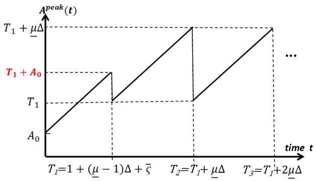
Figure 2. Peak AoI of Algorithm  2 in a line-type network.

As Algorithm  2 seeds in a round-robin way from a well-designed set $\Omega$ of seed candidates, one may imagine a periodic pattern of the peak AoI dynamics $A^{\rm peak}(t)=\max\limits_{v_{i}\in V}A(v_{i},t)$ in after some initial time under Algorithm  2. In fact, our later Theorem 4 will prove that this is true to follow Figure  2 with the periodic pattern since time $T_{1}$. To minimize the peak AoI in (9), we show, by the following Proposition 1 (with proof given in Appendix B.1), that it is equivalent to minimizing $1+(\underline{\mu}^{\prime}-1)\Delta+\overline{\varsigma}^{\prime}$ by choosing number $\underline{\mu}^{\prime}$ of seeds selected up to time $T_{1}$ in Step 2 of Algorithm  2.

Proposition 0.

In Algorithm  2, the optimal ($\underline{\mu},\overline{\varsigma}$) should be chosen by solving the following problem:

(16) $$\min\limits_{(\overline{\varsigma}^{\prime},\underline{\mu}^{\prime})}\quad T_{1}=1+(\underline{\mu}^{\prime}-1)\Delta+\overline{\varsigma}^{\prime}$$

(17) s.t. $$\underline{\mu}^{\prime}+\Delta(\underline{\mu}^{\prime}-1)\underline{\mu}^{\prime}+2\overline{\varsigma}^{\prime}\underline{\mu}^{\prime}\geq|diam(G)|+1,\quad$$

(18) $$0\leq\overline{\varsigma}^{\prime}<\Delta,$$

(19) $$\overline{\varsigma}^{\prime},\underline{\mu}^{\prime}{\rm\;are\;both\;integers},$$

in which (17) ensures that all nodes on $diam(G)$ are updated by time $T_{1}$. The optimal solution $(\overline{\varsigma},\underline{\mu})$ to Problem (16)-(19) is given by:

(20) $$\underline{\mu}=(\left\lfloor\frac{\Delta-1+\sqrt{\Delta^{2}+2\Delta+4|diam(G)|\Delta+1}}{2\Delta}\right\rfloor,$$

and

(21) $$\overline{\varsigma}=\left\lceil\frac{|diam(G)|+1-(\underline{\mu}^{2}\Delta-\underline{\mu}\Delta+\underline{\mu})}{2\underline{\mu}}\right\rceil).$$

In view of Proposition 1, the optimal solution ($\underline{\mu},\overline{\varsigma}$) to Problem (16)-(19) tells that Algorithm  2 achieves the earliest time when all each node on $diam(G)$ is updated. Given (20) and (21), we are ready to run Algorithm  2 optimally, where the configuration of each seed candidate $\omega_{x}=v_{\zeta(x)}$ in its Step 2 is finalized by: $\zeta(x)=\Delta(\underline{\mu}-x+1)^{2}+\underline{\mu}-x+1+(2\underline{\mu}-2x+1)\overline{\varsigma}$.

4.1. Approximation Analysis in Line-type Networks

To evaluate the approximation guarantee achieved by Algorithm  2, we start off with a line-type (or linear) network topology as defined below. It is simple but fundamental to inspire our performance analysis in a general graph as discussed later in Section 4.2.

Definition 0 (Line-type social network (Krawczyk et al., 2011)).

A line-type social network consists of a set of sequentially connected users/nodes, which resembles a line.

Given the NP-hard nature of our peak AoI minimization problem (3), one can hardly find an optimal solution. Instead, we establish a lower bound approximation for the optimum solution by the following lemma (with its proof given in Appendix B.2), which draws upon our closed-form expression (9).

Lemma 0.

In line-type social networks, an optimal solution to the peak AoI minimization problem yields that

(22) $$A^{\rm peak}_{\rm OPT}\geq\max\{A_{0}+\overline{\varsigma},\left\lfloor{\xi}\right\rfloor\Delta\}+1+\underline{\mu}\Delta.$$

in which $\xi=\frac{-(1+3\Delta)+\sqrt{(1+3\Delta)^{2}+4\Delta(1+2\underline{\mu}\Delta)}}{2\Delta}$.

In fact, Lemma 3 provides us with a comparison benchmark in deriving the approximation of our Algorithm  2, as discussed in the following Theorem 4 as proved in Appendix B.3.

Theorem 4.

For a line-type social network, Algorithm  2 runs in $O(mn)$-time and guarantees an approximation $\frac{1+2\underline{\mu}\Delta+\overline{\varsigma}}{1+\underline{\mu}\Delta+\left\lfloor{\xi}\right\rfloor\Delta}$ of the optimum, which is strictly smaller than 2. Particularly, Algorithm  2 is optimal for $n\leq\frac{A_{0}^{2}+A_{0}(1-\Delta)}{\Delta}$.

In view of Lemma 3, the low time complexity and approximation tell decent performances of our Algorithm  2, which even achieves optimality for small networks. It is worth noting that the de facto approximation of our Algorithm  2 especially for large networks could be improved by a math program as formulated in Appendix LABEL:appendix_improved_theorem_for_the.

4.2. Analysis Extension to General Social Networks

In general networks, social connections are more complicated and AoI updates among network nodes may become more interrelated. Note that Algorithm 2 solely seeds on the diameter of a general graph, making its corner nodes suffer from larger delay than its middle nodes. Besides, any social connection between nodes outside $diam(G)$ will evidently accelerate our algorithm’s information diffusion and consequently ameliorate our algorithm’s performance. As such, when analyzing Algorithm 2’s worst-case performance, it is sufficient to focus on the histogram (as defined below and shown in Figure 3) that is reduced from a given general graph. Our subsequent Theorem 7 corroborates this claim.

Definition 0 (Histogram-type graph $H(V_{H},E_{H})$).

In a histogram-type network $H(V_{H},E_{H})$, each node $v\in V_{H}$ follows

(23) $$\min\limits_{v^{\prime}\in diam(H)}dist(v^{\prime},v)\leq\min\{dist(v_{\perp},v_{\vdash}),dist(v_{\perp},v_{\dashv})\},$$

where $v_{\vdash}$ and $v_{\dashv}$ indicate the left- and the right-most nodes on the diameter path $diam(H)$ of graph $H$, respectively, and $v_{\perp}$ denotes the closest node to $v$ on $diam(H)$, i.e., $v_{\perp}\triangleq\arg\min\limits_{v^{\prime}\in diam(H)}dist(v^{\prime},v)$.

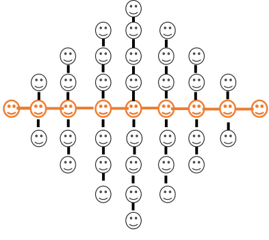
Figure 3. Illustration of a histogram network structure in which nodes on the diameter path are highlighted in orange.

Data: A general graph $\{G\}$.

Result: A reduced histogram graph $H(V_{H},E_{H})$ corresponding to $G$.

1 Find an arbitrary diameter path $diam(G)$ (if multiple exist) of the given graph $G$.

2 Let $V(diam(G))$ summarize those nodes that appear on $diam(G)$, and let $W\triangleq V-V(diam(G))$ summarize those nodes that do not appear on $diam(G)$.

3 Initialization. $V_{H}=V(diam(G)),E_{H}=E(diam(G))$.

4 forall $v_{i}\in W$ do

5       Find $v^{*}_{i}\triangleq\arg\min\limits_{v\in V_{H}}\{dist(v,v_{i})\}$ (if multiple $v^{*}_{i}$ exist, higher priority is given to a node on $diam(G)$).

6       Update $V_{H}=V_{H}+\{v_{i}\}$ and $E_{H}=E_{H}+\{(v_{i},v^{*}_{i})\}$.

7 end forall

Algorithm 3 Graph Reducing Approach

The following lemma with its proof moved to Appendix LABEL:apppendix_reduce_generagraph_lemma gives us a clue for subsequent approximation analysis.

Lemma 0.

The approximation of CyclicSelction in a general social network suffices from being checked in a histogram-type social network with the same diameter.

In Algorithm  3, we reduce a given general graph $G$ to a corresponding histogram graph $H(G)$, which eases our approximation analysis but has no bearing on our approximation result. At the high level, Algorithm 3 first copies $diam(G)$ to $H(G)$; then, for each node $v_{i}$ of $G$ but outside $diam(G)$, Algorithm 3 finds in the current node set $V_{H}$ the node $v^{*}_{i}$ that is closest to $v_{i}$ under graph $G$, and adds node $v_{i}$ and edge $(v_{i},v_{i}^{*})$ to $V_{H}$ and $E_{H}$ of graph $H(G)$, respectively.

Then it becomes tractable to analyze the performance of our Algorithm 3 for $H(G)$ here. Evidently, Algorithm 3’s peak AoI in general graphs would not exceed $A_{0}+diam(G)$. Considering the information diffusion among nodes solely on the diameter path of a general graph, one can also apply the right-hand-side of (22) in Lemma 3 as a lower bound on the optimum peak AoI for a general graph. Thus, one can obtain Algorithm  2’s approximation guarantee for general graphs in the following Theorem 7 (with proof moved to Appendix LABEL:appendix_general_peak_approximation).

Theorem 7.

For the peak AoI minimization problem (3), Algorithms  2 and  3 guarantee an approximation ratio

$$\frac{diam(G)+A_{0}}{\max\{A_{0}+\overline{\varsigma},\left\lfloor{\xi}\right\rfloor\Delta\}+1+\underline{\mu}\Delta}.$$

Next, we present our solution to the average AoI problem (4).

5. Average AoI Minimization Algorithms

Unlike the peak AoI problem (3), optimizing average AoI is more involved as it explicitly takes into account the AoI dynamics of every user. Despite our closed-form expression (10) of the average AoI objective in Theorem  7, finding a feasible solution to our problem is still challenging due to its NP-hard combinatorial nature.

Thereby, we equivalently transform the objective in (10) to the one in the following Proposition  1 (which is proved in Appendix  LABEL:appendix_proof_for_reformulated_avgaoi). With this transformation, we can develop efficient approximation algorithms that provide near-optimal solutions.

Proposition 0.

Given $S_{k}=(s_{1},...,s_{k})$ of dynamically selected seeds,

(24) $$\begin{split}A^{\rm avg}&=\eta+\frac{1}{n}\sum\limits_{v_{i}\in V}\Big{\{}\underbrace{2A_{0}\cdot[\Delta i_{1}+dist(s_{i_{1}},v_{i})]}_{\rm denoted\;as\;term\;1}\\ &\;\;\;+\underbrace{2\Delta\cdot\sum\limits_{j=1}^{k_{i}}[(i_{j}-i_{j-1})\cdot dist(s_{i_{j}},v_{i})]}_{\rm denoted\;as\;term\;2}+\underbrace{\Delta^{2}\sum\limits_{j=1}^{k_{i}}(i_{j}-i_{j-1})^{2}}_{\rm denoted\;as\;term\;3}\Big{\}},\end{split}$$

where $i_{0}=1$ initially, indices in set $\{i_{1},...i_{k_{i}}\}$ are obtained by running Algorithm  1 on $S_{k}$, and

(25) $$\eta=\frac{1}{2T}[2A_{0}-2\Delta A_{0}+T^{2}+2\Delta T+\Delta^{2}-2\Delta+2(\Delta-T\Delta-\Delta^{2})k+\Delta^{2}k^{2}].$$

As $\eta$ in (25) is a constant, we focus on the other three terms in (24) and aim to rigorously lower and upper bounding each of the three terms in (24) for further approximation analysis, respectively. Consequently, we have the following lemma (with its proof moved to Appendix LABEL:appendix_lemma_boundingterm1).

Lemma 0.

Given $S_{k}=(s_{1},...,s_{k})$, the followings hold:

$$A_{0}\Delta\leq A_{0}\cdot[i_{1}\Delta+dist(s_{i_{1}},v_{i})]\leq A_{0}\Delta+A_{0}\cdot dist(s_{1},v_{1}),$$

$${\color[rgb]{0,0,0}\Delta\cdot\sum\limits_{j=1}^{k}\frac{dist(s_{j},v_{i})}{\beta}}\leq\Delta\cdot\sum\limits_{j=1}^{k_{i}}[(i_{j}-i_{j-1})\cdot dist(s_{i_{j}},v_{i})]\leq\Delta\cdot\sum\limits_{j=1}^{k}dist(s_{j},v_{i}),$$

$$\frac{(k-1)^{2}\Delta^{2}}{2k_{i}}\leq\frac{1}{2}\Delta^{2}\sum\limits_{j=1}^{k_{i}}(i_{j}-i_{j-1})^{2}\leq{\color[rgb]{0,0,0}\frac{(k-1)^{2}\Delta^{2}}{2}},$$

where $\beta$ is the longest distance between a seed in $S_{k}$ and any node in $V$ and is less than $|diam(G)|$.

By applying Lemma 2 back to (24) of Proposition  1, we rigorously achieve a two-sided bound on the objective $A^{\rm avg}$ as in the following Theorem 3 (with its proof given in Appendix LABEL:avg_lowerbound_ratio_appendix).

Theorem 3.

Given $S_{k}=(s_{1},...,s_{k})$ of dynamically selected seeds, the average AoI objective (24) can be lower and upper bounded as:

(26) $$A^{\rm avg}\geq 2A_{0}\Delta+\frac{n(k-1)^{2}\Delta^{2}}{\sum\limits_{v_{i}\in V}k_{i}}+\frac{2\Delta}{n\beta}\sum\limits_{v_{i}\in V}\sum\limits_{s_{j}\in S_{k}}dist(s_{j},v_{i})+\eta,$$

and

(27) $$\begin{split}A^{\rm avg}\leq&2A_{0}\Delta+(k-1)^{2}\Delta^{2}+\frac{2A_{0}}{n}\sum\limits_{v_{i}\in V}dist(s_{1},v_{i})\\ &+\frac{2\Delta}{n}\sum_{v_{i}\in V}\sum_{s_{j}\in S_{k}}dist(s_{j},v_{i})+\eta.\end{split}$$

In the lower bound (26) and upper bound (27) above, we observe a common summation term $\sum\limits_{v_{i}\in V}\sum\limits_{s_{j}\in S_{k}}dist(s_{j},v_{i})$. This enables us to links our problem to the following Problem  1, which is significantly simplified and can be solved efficiently.

Problem 1 (Sum-distance minimization problem).

Given a graph $G(V,E)$, the objective is to select a subset $S\subseteq V$ with size $k$ to minimize the sum distance $\sum\limits_{s_{j}\in S_{k}}\sum\limits_{v_{i}\in V}dist(s_{j},v_{i})$.

Data: $G=(V,E)$, $k$.

Result: $S_{k}$.

1 Initialize the distance matrix $\bm{M_{G}}=(dist(v_{i},v_{j}))_{n\times n}$ of graph $G$ and unit vector $\bm{M_{1}}=(1)_{n\times 1}$.

2 Compute $\bm{M_{S}}\leftarrow\bm{M_{G}}\cdot\bm{M_{1}}$.

3 Find in $\bm{M_{S}}$ indices corresponding to the first $k$ smallest entries, resulting in sequence $\Theta$.

Select in set $V$ the $k$ nodes indexed by indices of $\Theta$ sequentially, forming $S_{k}$.

Algorithm 4 $k$-minisum for average AoI minimization

Our intriguing connection to Problem  1 successfully provides a tractable way for our algorithm design and approximation analysis. In Algorithm  4, we present our approach to minimizing $A^{\rm avg}$. Generally, Algorithm  4 first constructs the distance matrix $\bm{M_{G}}=(dist(v_{i},v_{j}))_{n\times n}$ that contains all pairwise shortest distances among nodes in the social network (Chan, 2012); then, according to the sum distance of a node over all the other nodes, Algorithm  4 seeds sequentially in decreasing order of nodes’ sum distances.

Theorem 4.

For the average AoI minimization problem (4), Algorithm  4 runs in $O(mn\cdot\frac{\log\log n}{\log n}+n^{2}\cdot\frac{\log^{2}\log n}{\log n})$-time, which is less than $O(mn)$, and guarantees an approximation ratio

$$\max\bigg{\{}\beta+\frac{A_{0}\beta}{k\Delta},\frac{2A_{0}\Delta+\eta+(k-1)^{2}\Delta^{2}}{2A_{0}\Delta+\eta+\frac{(k-1)^{2}\Delta^{2}}{k}}\bigg{\}}.$$

Proof.

The running time of Algorithm  4 is dominated by its Step 1 in returning all-pairs-shortest-path (APSP) distances of a given graph $G(V,E)$. Thanks to the state-of-art result for APSP (Chan, 2012), our Algorithm  4 totally runs in $O(mn\cdot\frac{\log\log n}{\log n}+n^{2}\cdot\frac{\log^{2}\log n}{\log n})$-time.

Next, we prove the approximation guaranteed by Algorithm  4. Denote $S_{k}=(s_{1},...,s_{k})$ and $S_{k}^{*}=(s_{1}^{*},...,s_{k}^{*})$ as the $k$ seeds that are dynamically-selected by Algorithm  4 and an optimal solution, respectively. Recall that $A^{\rm avg}_{\rm OPT}$ and $A^{\rm avg}_{\rm ALG}$ denote the average AoI results of an optimal solution and our algorithm, respectively. According to Theorem  3, we have

(28) $$A^{\rm avg}_{\rm OPT}\geq\underbrace{2A_{0}\Delta+\eta+\frac{n(k-1)^{2}\Delta^{2}}{\sum\limits_{v_{i}\in V}k_{i}^{*}}}_{{\rm denoted,\;for\;short,\;as\;}A^{\rm avg}_{\rm OPT}|_{1}}+\underbrace{\frac{2\Delta}{n\beta}\sum\limits_{v_{i}\in V}\sum\limits_{s_{j}^{*}\in S_{k}^{*}}dist(s_{j}^{*},v_{i})}_{{\rm denoted,\;for\;short,\;as\;}A^{\rm avg}_{\rm OPT}|_{2}},$$

(29) $$\begin{split}A^{\rm avg}_{\rm ALG}\leq&\underbrace{2A_{0}\Delta+(k-1)^{2}\Delta^{2}+\eta}_{{\rm denoted,\;for\;short,\;as\;}A^{\rm avg}_{\rm ALG}|_{1}}\\ &+\underbrace{\frac{2A_{0}}{n}\sum\limits_{v_{i}\in V}dist(s_{1},v_{i})+\frac{2\Delta}{n}\sum_{v_{i}\in V}\sum_{s_{j}\in S_{k}}dist(s_{j},v_{i})}_{{\rm denoted,\;for\;short,\;as\;}A^{\rm avg}_{\rm ALG}|_{2}}.\end{split}$$

By applying (28) and (29) into (6), we further obtain

(30) $$\begin{split}\frac{A^{\rm avg}_{\rm ALG}}{A^{\rm avg}_{\rm OPT}}\leq\frac{A^{\rm avg}_{\rm ALG}|_{1}+A^{\rm avg}_{\rm ALG}|_{2}}{A^{\rm avg}_{\rm OPT}|_{1}+A^{\rm avg}_{\rm OPT}|_{2}}\leq\max\{\frac{A^{\rm avg}_{\rm ALG}|_{1}}{A^{\rm avg}_{\rm OPT}|_{1}},\frac{A^{\rm avg}_{\rm ALG}|_{2}}{A^{\rm avg}_{\rm OPT}|_{2}}\},\end{split}$$

where the first inequality holds by (28) and (29), and the second inequality is due to the fact that $\frac{x_{1}+x_{2}}{y_{1}+y_{2}}\leq\max\{\frac{x_{1}}{y_{1}},\frac{x_{2}}{y_{2}}\}$ holds for any four positive numbers $x_{1},y_{1},x_{2},y_{2}$. On one hand, note that the seed set $S_{k}$ selected by our Algorithm  4 also minimizes Problem  1, i.e.,

(31) $$\sum_{v_{i}\in V}\sum_{s_{j}\in S_{k}}dist(s_{j},v_{i})\leq\sum_{v_{i}\in V}\sum_{s_{j}^{*}\in S_{k}^{*}}dist(s_{j}^{*},v_{i}).$$

Due to Step 3 of our Algorithm  4, we have on the other hand that

(32) $$\sum\limits_{s_{j}\in S_{k}}\sum\limits_{v_{i}\in V}dist(s_{j},v_{i})\geq k\cdot\sum\limits_{v_{i}\in V}dist(s_{1},v_{i}).$$

Considering the fact that $\sum\limits_{v_{i}\in V}dist(s_{1},v_{i})\leq\sum\limits_{v_{i}\in V}dist(s_{j},v_{i})$ holds for each $s_{j}\in S_{k}$, the following which stems from (28) and (29) holds:

(33) $$\begin{split}\frac{A^{\rm avg}_{\rm ALG}|_{2}}{A^{\rm avg}_{\rm OPT}|_{2}}&\leq\frac{(\frac{2A_{0}}{nk}+\frac{2\Delta}{n})\cdot\sum\limits_{v_{i}\in V}\sum\limits_{s_{j}\in S_{k}}dist(s_{j},v_{i})}{\frac{2\Delta}{n\beta}\sum\limits_{v_{i}\in V}\sum\limits_{s_{j}^{*}\in S_{k}^{*}}dist(s_{j}^{*},v_{i})}\\ &\leq\frac{(\frac{2A_{0}}{nk}+\frac{2\Delta}{n})\cdot\sum\limits_{v_{i}\in V}\sum\limits_{s_{j}^{*}\in S_{k}^{*}}dist(s_{j}^{*},v_{i})}{\frac{2\Delta}{n\beta}\sum\limits_{v_{i}\in V}\sum\limits_{s_{j}^{*}\in S_{k}^{*}}dist(s_{j}^{*},v_{i})}=\frac{A_{0}\beta}{k\Delta}+\beta,\end{split}$$

in which the first and the second inequalities are due to (32) and (31), respectively. Since $\sum\limits_{v_{i}\in V}k^{*}_{i}\leq\sum\limits_{v_{i}\in V}k=nk$, we also have

(34) $$\frac{A^{\rm avg}_{\rm ALG}|_{1}}{A^{\rm avg}_{\rm OPT}|_{1}}\leq\frac{2A_{0}\Delta+(k-1)^{2}\Delta^{2}+\eta}{2A_{0}\Delta+\eta+\frac{n(k-1)^{2}\Delta^{2}}{\sum\limits_{v_{i}\in V}k_{i}^{*}}}\leq\frac{2A_{0}\Delta+\eta+(k-1)^{2}\Delta^{2}}{2A_{0}\Delta+\eta+\frac{(k-1)^{2}\Delta^{2}}{k}}$$

By applying (33) and (34) to (30), the proof completes. ∎

Theorem 4 demonstrates that the performance gap between our algorithm and the optimum is not big and does not increase rapidly with the size of the social network. The value of $\beta$ in the approximation guarantee is much smaller than the diameter of the network, which tells our algorithm’s good approximation performance even for large networks. The approximation guarantee also tells that expanding the time horizon $T=1+(k-1)\Delta$ with more promotion updates $k$ will narrow the gap between our algorithm’s solution and the optimum, yielding our solution’s better approximation performance. This is because larger $T$ will lead to a larger $\eta$, which is a common part of the average AoI under any solution.

6. Experiments

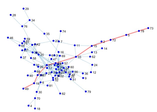
Figure 4. Social network visualization.

In this section, we empirically evaluate our algorithms by experiments on a real data set of Facebook social circles (Leskovec and Mcauley, 2012; Stanford, 2023). In the following implementation, we consider the typical 100 users with their IDs $\{1,2,...,100\}$ in the original data set (Leskovec and Mcauley, 2012; Stanford, 2023), from which we remove some isolated users that have no bearing on our experiment results. Consequently, our social network $G(V,E)$ is visualized in Figure  4, where the diameter path $diam(G)$ is highlighted in thick red.

Since it is NP-hard to find optimal $A^{\rm peak}_{\rm OPT}$ and $A^{\rm avg}_{\rm OPT}$, we are inspired by Theorems  6 and 9 to apply the following lower bounds ${\rm LB_{peak}}$ and ${\rm LB_{avg}}$ as our algorithms’ comparison benchmarks, respectively:

(35) $$\begin{split}{\rm LB}_{\rm peak}&=A_{0}+1+\frac{1}{n(n-1)}\sum\limits_{v_{j}\in V}\sum\limits_{v_{i}\in V-\{v_{j}\}}dist(v_{j},v_{i})\\ &\leq A_{0}+1+\max\limits_{v_{i},v_{j}\in V}\{dist(v_{j},v_{i})\}\overset{(\ref{eq_peak_vi})}{\leq}A^{\rm peak}_{\rm OPT}.\end{split}$$

(36) $${\rm LB_{avg}}=2A_{0}\Delta+\eta+\frac{(k-1)^{2}\Delta^{2}}{k}+\frac{2\Delta P_{1}(G)}{n\cdot|diam(G)|}\overset{(\ref{lowerbound_eq_avg})}{\leq}A^{\rm avg}_{\rm OPT},$$

where $\eta$ refers to (25) and $P_{1}(G)\triangleq\min\limits_{V^{\prime}\subseteq V,|V^{\prime}|=k}\sum\limits_{v_{i}\in V}\sum\limits_{v_{j}\in V^{\prime}}dist(v_{i},v_{j})$ indicates the optimum of the sum-distance minimization problem in Problem 1 on graph $G$. It is important to note that both ${\rm LB_{peak}}$ and ${\rm LB_{avg}}$ are independent of how an optimal solution seeds, since they are general lower bounds on our peak and average AoI objectives.

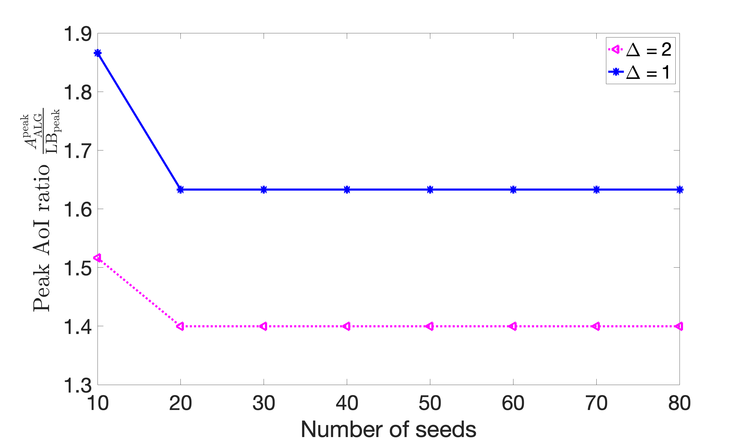
Figure 5. Peak AoI performance ratio $\frac{A^{\rm peak}_{\rm ALG}}{{\rm LB}_{\rm peak}}$.

For peak AoI minimization, we implement our Algorithm 2 with different settings of the seeding interval $\Delta=1$ and $\Delta=2$, respectively, and vary the time horizon till $T=80$ time slots. Our experiment results are presented in Figure  5. Since our empirical peak AoI ratio in Figure  5 is close to one, telling the near-optimal performance of our Algorithm 2 in practical scenarios. The reason for the early drop in Figure  5 is two-fold: first, our benchmark ${\rm LB_{peak}}$ is chosen as a constant value that is smaller than $A^{\rm peak}_{\rm OPT}$; second, our algorithm could achieve better performance when the overall seed number $k$ increases in an early stage. Once $k$ rises above a threshold 20, our empirical peak AoI ratio’s pattern decreases as the time horizon $T=1+(k-1)\Delta$ expands. This validates our theoretical finding as aforementioned in Section 4 that Algorithm 2 results in a periodic pattern in its peak AoI dynamics. Recall in Proposition 1 that the optimized $\underline{\mu}$ in (20) decreases as $\Delta$ increases, i.e., our Algorithm 2 selects fewer candidates on $diam(G)$ as seeding interval $\Delta$ enlarges. This implies that larger $\Delta$ will induce a larger peak AoI approximation in our Algorithm 2, as shown in Figure  5.

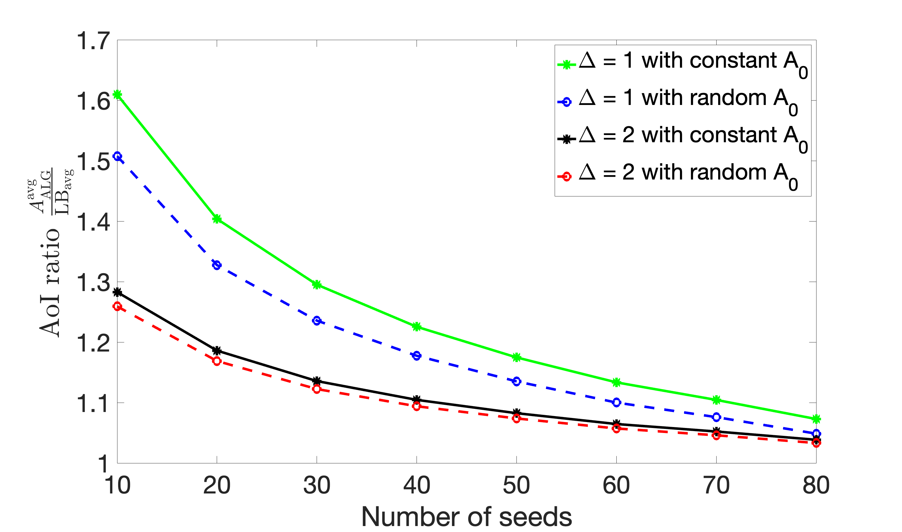
Figure 6. Average AoI performance $\frac{A^{\rm avg}_{\rm ALG}}{{\rm LB}_{\rm avg}}$.

For average AoI minimization, we not only evaluate our solutions under constant initial age $A_{0}$ as modeled in Section  2, but also extends to a more general setting where users’ different initial ages are randomly generated with the mean equal to the constant $A_{0}$. We test our Algorithm  4 by varying the time horizon till $T=80$ time slots and present corresponding experiment results in Figure  6, by comparing with the optimum’s lower bound (36) in a ratio. Regardless of random or deterministic $A_{0}$ distribution for each user, Figure  6 shows that our Algorithm  4’s empirical average AoI ratio is small and close to one, revealing Algorithm  4’s near-optimal performance in practical scenarios. As seed number $k$ or time horizon $T$ increases with more information updates, the ratio telling the performance gap between our Algorithm  4 and the optimum (bound) further reduces. This also corroborates our theoretical findings in Theorem 4 as aforementioned in Section 5.In addition, Figure  6 shows that our Algorithm  4 performs even better as the seeding interval $\Delta$ increases since larger $\Delta$ creates more opportunities for us to chase the optimal $A^{\rm avg}_{\rm OPT}$ by diffusing to more nodes in each seeding interval.

7. Concluding Remarks

To the best of our knowledge, we initiate the theoretical study of optimizing information diffusion on social networks with a multi-stage seeding process. By considering a coupling metric bridging AoI and approximation analysis, we comprehensively study two objectives (i.e., the peak and average AoI) of the problem and prove that our problem is NP-hard in general. As a critical step, we first manage to derive closed-form expressions that trace the AoI dynamics of the network, which is highly non-trivial due to a multi-stage seeding process and the involved topology of a general social network. By focusing on a fine-tuned set of seed candidates on the diameter path, we design a fast algorithm that guarantees decent approximations as compared to the optimum for the peak AoI minimization problem. To minimize the average AoI, we develop a new framework that allows for algorithm design and approximation analysis, which benefits from our rigorous two-side bound analysis on the average AoI objective. Our framework enables us to achieve a polynomial-time algorithm that guarantees a good approximation. Our theoretical findings are corroborated by experiments that are conducted on a real social network.

Appendix A Missed Proofs in Section  3

A.1. Proof of Lemma  1

Proof.

Recall that the AoI of each node $v_{i}$ will increase linearly in each time slot $[t,t+1)$ for $t=\{0,...,T-1\}$, see Section  2. Given the set $S_{x}$ of dynamically selected seed nodes, we now discuss in the following the AoI of a node $v_{i}$ at an integer time point $\overline{t}$, i.e., $A(v_{i},\overline{t})$. Since $A(v_{i},0)=A_{0}$, we only need to discuss the AoI of $v_{i}$ at time $\overline{t}\in\{1,...,T-1\}$. Accordingly, we discuss the following two cases.

Case 1. $\Omega(v_{i},\overline{t})$ is empty.

Since no seed is available to update $v_{i}$ at time $\overline{t}$, the AoI of $v_{i}$ will increase linearly based on $A(v_{i},\overline{t}-1)$, i.e.,

(37) $$A(v_{i},\overline{t})=A(v_{i},\overline{t}-1)+1.$$

Case 2. $\Omega(v_{i},\overline{t})$ is not empty.

There exist seeds from set $\Omega(v_{i},\overline{t})$ that update de facto the AoI of $v_{i}$ at time $\overline{t}$. Further, $A(v_{i},\overline{t})$ will be updated by the freshest information up to time $\overline{t}$. Accordingly, we have

(38) $$A(v_{i},\overline{t})=\min\limits_{s_{x}\in\Omega}\{1+\overline{t}-t_{x}\}=\min\limits_{s_{x}\in\Omega}\{1+dist(v_{i},s_{x})\},$$

where the second equation is due to the fact that $\overline{t}=t_{x}+dist(s_{x},v_{i})$. In summary, we have the AoI of $v_{i}$ at an arbitrary integer time point $\overline{t}$ as follows:

(39) $$A(v_{i},\overline{t})=\left\{\begin{matrix}A_{0},&{\rm\;if\;}\overline{t}=0,\\ A(v_{i},\overline{t}-1)+1,&{\rm\;if\;}\overline{t}\geq 1{\rm\;and\;}\Omega(v_{i},\overline{t})=\varnothing,\\ \min\limits_{s_{x}\in\Omega(v_{i},\overline{t})}\{1+dist(v_{i},s_{x})\},&{\rm\;if\;}\overline{t}\geq 1{\rm\;and\;}\Omega(v_{i},\overline{t})\neq\varnothing.\end{matrix}\right.$$

Furthermore, at an arbitrary time $t$, $A(v_{i},t)$ (i.e., the AoI of an arbitrary node $v_{i}$) can be written as shown in Lemma  1. ∎

A.2. Missed Proof in Lemma  3

Proof.

Note that, within the time horizon $[0,T]$, $A(v_{i},t)$ drops only when $v_{i}$ is updated its AoI by some seed. Since each seed $s_{x}\in S_{k}$ is selected at timestamp $t_{x}$ and the AoI of $v_{i}$ takes unit time to disseminate along each edge, $v_{i}$ would be updated by $s_{x}$ at time $t_{x}+dist(s_{x},v_{i})$. This further implies that any discontinuity point of $v_{i}$ can be found in the following set

(40) $$\{t_{x}+dist(s_{x},v_{i})|x\in{1,...,k}\}.$$

This concludes the proof. ∎

A.3. Missed Proof in Lemma  4

Proof.

According to Definition  1, we know that a time point $t_{j}+dist(s_{j},v_{i})$ is not a discontinuity point if

(41) $$\Omega(v_{i},t_{j}+dist(s_{j},v_{i}))=\varnothing.$$

Since $1\leq t_{j}<t_{j}+dist(s_{j},v_{i})$, we further have

(42) $$\begin{split}&\Omega(v_{i},t_{j}+dist(s_{j},v_{i}))=\varnothing\\ &\Rightarrow dist(v_{i},s_{j})\geq A(v_{i},t_{j}+dist(s_{j},v_{i})-1)\\ &\Rightarrow\underbrace{1+dist(v_{i},s_{j})}_{{\rm AoI\;of\;}s_{j}{\rm\;at\;}t_{j}+dist(s_{j},v_{i})}\geq\underbrace{A(v_{i},t_{j}+dist(s_{j},v_{i})-1)+1}_{{\rm AoI\;of\;some\;other\;source\;at\;}t_{j}+dist(s_{j},v_{i})}.\end{split}$$

implying that there exists a seed node, denoted as $s_{y}$, that is selected later than $s_{j}$ but diffuses its information to $v_{i}$ no later than time $t_{j}+dist(s_{j},v_{i})$, i.e.,

(43) $$t_{y}>t_{j}{\rm\;and\;}t_{y}+dist(s_{y},v_{i})\leq t_{j}+dist(s_{j},v_{i}).$$

This completes our proof. ∎

A.4. Improved Discontinuity Points Finder

Note that our Algorithm  1 only removes, in each iteration of its nested for-loop, at most one element from $\{t_{x}+dist(s_{x},v_{i})|x\in[k]\}$, leading to low time-efficiency in most cases.

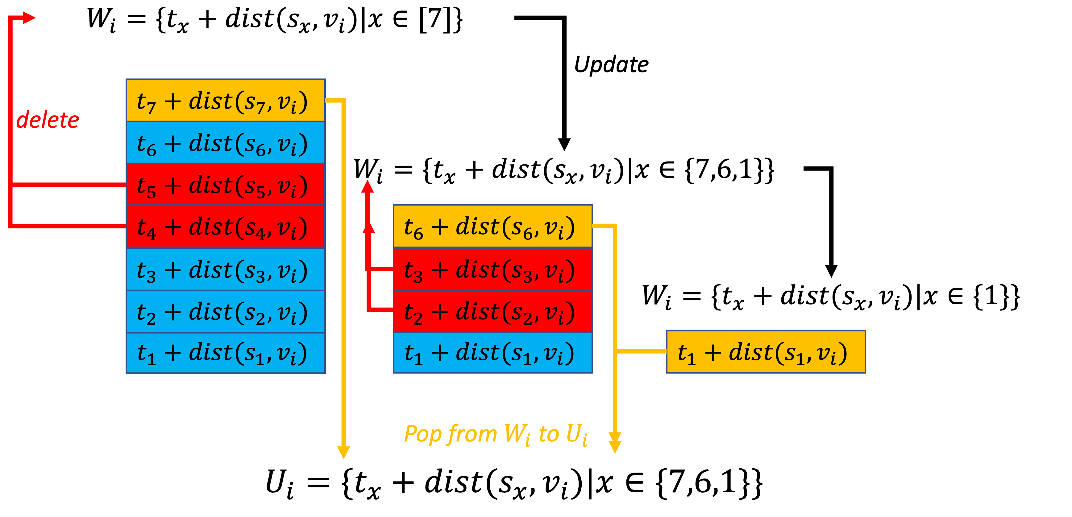
Figure 7. Illustration example of Algorithm  5, where $k=7$, $t_{1}+dist(s_{1},v_{i})<t_{6}+dist(s_{6},v_{i})<t_{2}+dist(s_{2},v_{i})<t_{3}+dist(s_{3},v_{i})<t_{7}+dist(s_{7},v_{i})<t_{4}+dist(s_{4},v_{i})<t_{5}+dist(s_{5},v_{i})$.

Data: $v_{i}\in V$, $S_{k}=\{s_{1},...,s_{k}\}$.

Result: $U_{i}$.

1 Initialization. $U_{i}\leftarrow\varnothing$, $W_{i}\leftarrow\{t_{x}+dist(s_{x},v_{i})|x\in[k]\}$.

2 while $W_{i}\neq\varnothing$ do

3       Find among elements in $W_{i}$ the index $l\triangleq\arg\max\limits_{t_{x}+dist(s_{x},v_{i})\in W_{i}}\{x\}$.

4       Update $U_{i}\leftarrow U_{i}+\{t_{l}+dist(s_{l},v_{i})\}$ and $W_{i}\leftarrow W_{i}-\{t_{l}+dist(s_{l},v_{i})\}$.

5       forall $t_{x}+dist(s_{x},v_{i})\in W_{i}$ do

6             if $t_{x}+dist(s_{x},v_{i})\geq t_{l}+dist(s_{l},v_{i})$ then

7                   Update $W_{i}\leftarrow W_{i}-\{t_{x}+dist(s_{x},v_{i})\}$.

8             end if

9            

10       end forall

11      

12 end while

Algorithm 5 Improved Discontinuity Finder

Below, we introduce a new Algorithm  5 that could remove several non-discontinuity points from $\{t_{x}+dist(s_{x},v_{i})|x\in[k]\}$ at each iteration, which significantly improves de facto the efficiency of Algorithm  1 in average cases.

Basically, our new Algorithm  5 finds all the discontinuity points of $v_{i}$ one by one in decreasing order of their corresponding time. More specifically, Algorithm  5 first initializes a stack $W_{i}$ which is constructed by pushing elements in $\{t_{x}+dist(s_{x},v_{i})|x\in[k]\}$ sequentially in increasing order of $x$ (the index of the seed leading to the potential discontinuity point). In each iteration, Algorithm  5 pops the top element, which is denoted as $t_{l}+dist(s_{l},v_{i})$, from the stack. Since $t_{l}+dist(s_{l},v_{i})$ corresponds to the seed $s_{l}$ with the freshest information among the others of $W_{i}$, it is de facto a discontinuity point due to Lemma  4. For each $t_{x}+dist(s_{x},v_{i})\in W_{i}$, its corresponding seed $s_{x}$ does not update $v_{i}$ if $t_{x}+dist(s_{x},v_{i})\geq t_{l}+dist(s_{l},v_{i})$. This is because that $s_{l}$ has updated $v_{i}$ some fresher information than $s_{x}$ by time $t_{x}+dist(s_{x},v_{i})$. With this observation, we remove, by the for-loop of Algorithm  5, all such elements from $W_{i}$. The algorithm iterates until finding all discontinuity points of $v_{i}$ when $W_{i}=\varnothing$. An example of Algorithm  5 can be found in Figure  7.

A.5. Missed Proof in Theorem  6

Proof.

Given $S_{k}$ of selected seeds, we first discuss the peak AoI of an arbitrary node $v_{i}\in V$. By Proposition  5, we know that the $A(v_{i},t)$ achieves a supremum at the right-endpoint in each of the following time intervals, respectively.

(44) $$\begin{split}&[0,t_{i_{1}}+dist(s_{i_{1}},v_{i})),\\ &[t_{i_{1}}+dist(s_{i_{1}},v_{i}),t_{i_{2}}+dist(s_{i_{2}},v_{i}))\\ &,...,\\ &[t_{i_{k_{i}-1}}+dist(s_{i_{k_{i}-1}},v_{i}),t_{i_{k_{i}}}+dist(s_{i_{k_{i}}},v_{i})),\\ &[t_{i_{k_{i}}}++dist(s_{i_{k_{i}}},v_{i}),T].\end{split}$$

With this insight, we further get

(45) $$\begin{split}A_{i}^{\rm peak}&=\sup\limits_{t\in[0,T]}\{A(v_{i},t)\}\\ &=\max\{\max\limits_{j\in\{1,...,k_{i}\}}\{A(v_{i},t_{i_{j}}+dist(s_{i_{j}},v_{i}))\},A(v_{i},T)\}.\end{split}$$

By substituting (45) back to (1), the $A^{\rm peak}$ over the time horizon $[0,T]$ can be expressed as follows

(46) $$\begin{split}A^{\rm peak}=\max\limits_{v_{i}\in V}\{A^{\rm peak}_{i}\}=(\ref{eq_peak_vi}),\end{split}$$

in which the second equation is due to Equation (8). ∎

A.6. Missed Proof in Theorem  7

Proof.

According to (2), we have

(47) $$A^{\rm avg}=\frac{1}{nT}\sum\limits_{v_{i}\in V}\int_{t=0}^{T}A(v_{i},t)dt.$$

Note that $A(v_{i},t)$ is a non-negative piece-wise function over the whole time horizon $[0,T]$. Given $S_{k}$ of dynamically selected seeds, we first look at the average AoI of a node $v_{i}\in V$. To this end, we partition the horizon $[0,T]$ into the following three intervals

(48) $$\begin{split}&[0,t_{i_{1}}+dist(s_{i_{1}},v_{i})),\\ &[t_{i_{1}}+dist(s_{i_{1}},v_{i}),t_{i_{k_{i}}}+dist(s_{i_{k_{i}}},v_{i})),\\ &[t_{i_{k_{i}}}+dist(s_{i_{k_{i}}},v_{i}),T].\end{split}$$

Due to Proposition  5, we now take integrals of function $A(v_{i},t)$ over the three intervals above in the above (48), respectively:

(49) $$\int\limits_{t=0}^{t_{i_{1}}+dist(s_{i_{1}},v_{i})}A(v_{i},t)dt=\frac{(t_{i_{1}}+dist(s_{i_{1}},v_{i}))\cdot(2A_{0}+t_{i_{1}}+dist(s_{i_{1}},v_{i}))}{2},$$

and

(50) $$\int\limits_{t=t_{i_{1}}+dist(s_{i_{1}},v_{i})}^{t_{i_{k_{i}}}+dist(s_{i_{k}},v_{i})}A(v_{i},t)dt=\sum\limits_{j=2}^{i_{k_{i}}}\frac{(2+2\cdot dist(s_{i_{j-1}},v_{i})+\Lambda_{ij})\cdot\Lambda_{ij}}{2},$$

where for $\Lambda_{ij}=t_{i_{j}}-t_{i_{j-1}}+dist(s_{i_{j}},v_{i})-dist(s_{i_{j-1}},v_{i})$ holds for each $j\in\{2,...,k_{i}\}$, and

(51) $$\begin{split}&\int_{t=t_{i_{k_{i}}}+dist(s_{i_{k_{i}}},v_{i})}^{T}A(v_{i},t)dt\\ &=\frac{(T-t_{i_{k_{i}}}-dist(s_{i_{k_{i}}},v_{i}))\cdot(3+2\cdot dist(s_{i_{k_{i}}},v_{i}))}{2}.\end{split}$$

By applying (49),(50), and (51) to Equation (47), the average AoI of the network follows

(52) $$\begin{split}&A^{\rm avg}\\ &=\frac{1}{nT}\sum_{v_{i}\in V}\int_{t=0}^{T}A(v_{i},t)dt\\ &=\frac{1}{nT}\sum_{v_{i}\in V}\sum\limits_{j=1}^{k_{i}+1}\frac{(2A_{i{j-1}}+\Lambda_{ij})\cdot\Lambda_{ij}}{2},\end{split}$$

in which $A_{ij}$ and $\Lambda_{ij}$ refer to Equation (11) and Theorem 7, respectively. The proof completes. ∎

A.7. Missed Proof in Theorem  10

Proof.

The NP-hardness of the average AoI minimization problem is shown by a reduction from the well-known NP-hard set cover problem. Given a ground set $U=\{u_{1},...,u_{q}\}$ of $q$ elements and a collection $\mathcal{U}=\{U_{1},...,U_{p}\}$ of $p$ subsets of $U$, the set cover problem aims to find $k$ ($<p$) subsets from $\mathcal{U}$ such that their union is equal to $U$. Given an instance of the set cover problem, we construct a graph of our problem by the following steps, where we set $T=3$ and $\Delta\rightarrow 0$.

• Step 1. Construct a set $V_{1}$ of $q$ nodes that correspond to those $q$ elements in the ground set $U$, respectively. Please refer to the top row of circles in Figure  8.

• Step 2. Construct a set $V_{2}$ of $p$ nodes that correspond to those $p$ subsets in $\mathcal{U}$, respectively. Please refer to those rectangles in the middle of Figure  8.

• Step 3. For each $u_{x}\in V_{1}$ and each $U_{y}\in V_{2}$, an edge $(u_{x},U_{y})$ is constructed if $u_{x}\in U_{y}$. Accordingly, we obtain our first edge set as $E_{1}$.

• Step 4. Find, in the current graph $G(V_{1}\cup V_{2},E_{1})$, the maximum degree of a node of $V_{1}$, which is denoted as

  (53) $$\alpha=\max\limits_{u_{x}\in V_{1}}\{deg(u_{x})\}.$$

  For each $U_{y}\in V_{2}$, we construct a set $\{v^{y}_{1},...,v^{y}_{\alpha+1}\}$ of ($\alpha+1$) dummy nodes that correspond to $U_{y}$. Accordingly, we obtain another node set $V_{3}$ consisting of all the dummy nodes, i.e.,

  $$V_{3}\triangleq\mathop{\cup}\limits_{j\in[p]}\{v^{j}_{1},...,v^{j}_{\alpha+1}\}$$

  .

• Step 5. For each $U_{y}\in V_{2}$ and each $v\in V_{3}$, we construct an edge $(U_{y},v)$. Accordingly, we have another edge set $E_{2}$.

By the five steps above, we obtain our graph as $G(V_{1}\cup V_{2}\cup V_{3},E_{1}\cup E_{2})$. Figure  8 illustrates an example of our graph construction that is converted from the set cover problem (where $U=\{u_{1},u_{2},....,u_{5}\}$, $\mathcal{U}=\{\{u_{1},u_{3},u_{5}\},\{u_{2},u_{4}\},\{u_{3},u_{5}\}\}$, and $k=2$).

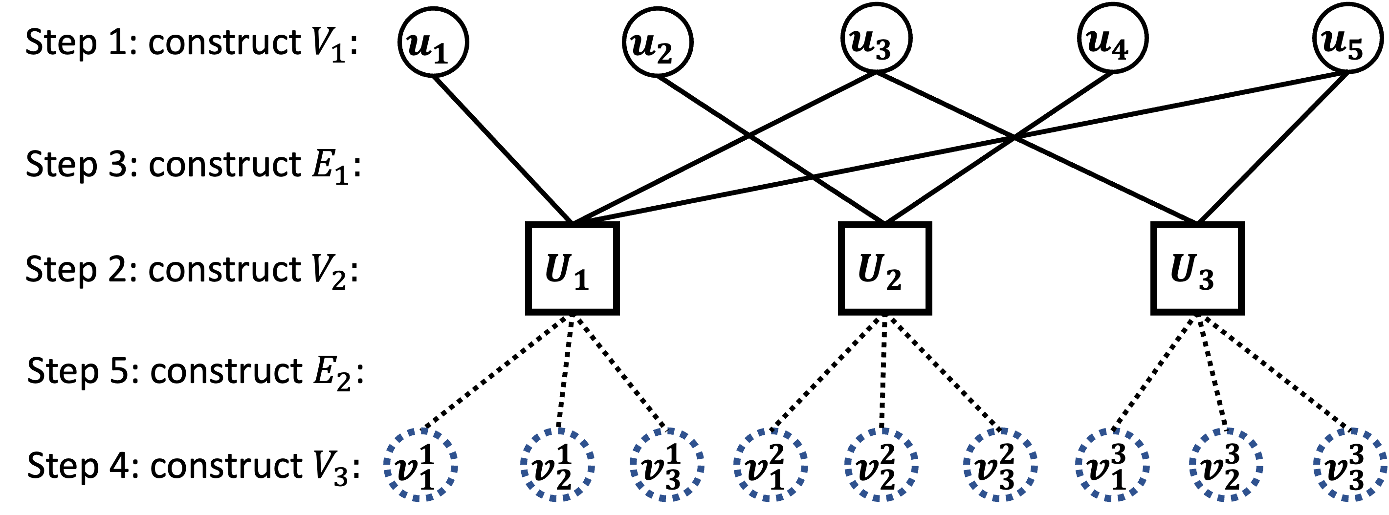
Figure 8. The graph converted from the set cover problem.

Now, we consider the average AoI of our graph $G(V_{1}\cup V_{2}\cup V_{3},E_{1}\cup E_{2})$. Since $\Delta\rightarrow 0$, the $k$ seeds could be regarded to be selected together, implying by Lemma  3 that the AoI of each node in $G(V_{1}\cup V_{2}\cup V_{3},E_{1}\cup E_{2})$ drops at most once in the time horizon $[0,3)$. For ease of exposition, we partition nodes in the graph into the following types according to their average AoI (as per Theorem  6).

• Nodes of type one refer to those seed nodes that share a common average AoI as $\frac{A_{0}+A_{0}+1}{2}+\frac{(1+3)\cdot 2}{2}=A_{0}+4.5$. Clearly, there are $k$ nodes of type one.

• Nodes of type two refer to those non-seed nodes that have at least one neighbor node selected as a seed, i.e., type-two nodes share a common average AoI as $2A_{0}+4.5$. Totally, there are are $|N_{G}(S_{k})|$ nodes of type two.

• Nodes of type three refer to those non-seed nodes that have no neighbor node selected as a seed. That is, type-three nodes share a common average AoI as $3A_{0}+4.5$. Totally, the number of type three nodes is

  (54) $$q+(\alpha+2)\cdot p-k-|N_{G}(S_{k})|.$$

By Theorem  7, we further have

(55) $$\begin{split}&A^{\rm avg}\\ &=\frac{4.5(2p+p\alpha+q)+A_{0}(6p+3\alpha p+3q-2k-|N_{G}(S_{k})|)}{3q+3p\alpha+6p}\\ &=\frac{(9+4.5\alpha+6A_{0}+3\alpha A_{0})p+(4.5+3A_{0})q-2A_{0}k-A_{0}\cdot|N_{G}(S_{k})|}{3q+3p\alpha+6p}\\ &=C_{1}-C_{2}\cdot|N_{G}(S_{k})|,\end{split}$$

in which

$$C_{1}=\frac{1}{3q+3p\alpha+6p}\cdot[(9+4.5\alpha+6A_{0}+3\alpha A_{0})p+(4.5+3A_{0})q-2A_{0}k]$$

and $C_{2}=\frac{A_{0}}{3q+3p\alpha+6p}>0$ are both constant. The following proposition characterizes an optimal solution of ours.

Proposition 0.

In our average AoI minimization problem (that is converted from the set cover problem), an optimal solution only seeds in $V_{2}$.

Proof of Proposition 1.

For sake of contradiction, suppose that there exists an optimal solution that seeds some $s_{j}$ which is not in $V_{2}$, i.e., $s_{j}\in V_{1}\cup V_{3}$. For analytical tractability, we denote $\overline{V_{2}}\triangleq V_{2}-V_{2}\cap S_{k}$ as the set of nodes in $V_{2}$ that are not selected as seeds. Note that $p>k$, which tells $\overline{V_{2}}\neq\varnothing$. Denote the set of nodes in $V_{2}$ that are associated with $v_{j}$ as

(56) $$\widetilde{V_{2}}(v_{j})\triangleq\{U_{x}\in V_{2}|(U_{x},v_{j})\in E_{1}\cup E_{2}\}.$$

Beow, we discuss two cases.

Case 1. (There exists a node in the intersection $\widetilde{V_{2}}(v_{j})\cap\overline{V_{2}}$, say $U_{x}$, that is associated with $v_{j}$ but not selected as a seed)

By seeding $U_{x}$ as the $j$-th seed $s_{j}$ instead, we know $|N_{G}(S_{k})|$ does not decrease since the $U_{x}$ is the only neighbor of the old $s_{j}$.

Case 2. ($\widetilde{V_{2}}(v_{j})\cap\overline{V_{2}}=\varnothing$)

According to the pigeonhole principle, we know that there exists at least one node in $\overline{V}_{2}$, say $U_{y}$, such that none of its corresponding nodes in $\{v^{y}_{1},...,v^{y}_{\alpha+1}\}$ is selected as a seed. By seeding $U_{y}$ as $s_{j}$, Further, we know that $|N_{G}(S_{k})|$ increase by at least one, which is because

$$deg(v_{j})\leq\alpha<\alpha+1=deg(U_{y})$$

where $deg(v)$ indicates the number of edges that are incident to a vertex $v$. Hence, according to (55), we know that the average AoI of the network will increase when replacing a seed outside $V_{2}$ by someone in $V_{2}$.

This concludes the proof. ∎

With Proposition  1, Equation (55) is equivalent to

(57) $$A^{\rm avg}=C_{1}-C_{2}\cdot[(\alpha+1)\cdot k+|N_{G}(S_{k})\cup V_{1}|]$$

Since $C_{2}=C_{1}-C_{2}\cdot k\cdot(\alpha+1)$ in (57) is a constant, $A^{\rm avg}$ decreases linearly with $|N_{G}(S_{k})\cup V_{1}|$ (which indicates the number of nodes in $V_{1}$ that are associated with at least one selected node in $V_{2}$). Hence,

(58) $$\begin{split}&\arg\min\limits_{S_{k}\subseteq V_{1}\cup V_{2}\cup V_{3},|S_{k}|=k}A^{\rm avg}(S_{k})\\ &=\arg\max\limits_{S_{k}\subseteq V_{1}\cup V_{2}\cup V_{3},|S_{k}|=k}|N_{G}(S_{k})\cup V_{1}|,\end{split}$$

indicating that an optimal solution to our problem is exactly an optimal solution to the given set cover problem. ∎

Appendix B Missed Proof in Section 4

B.1. Missed Proof in Proposition 1

Proof.

Intuitively, Problem (16)-(19) in Proposition 1 tries to minimize the earliest time (denoted as $T_{1}$) when all nodes on the diameter path $diam(G)$ is updated.

Suppose, w.l.o.g., that $T_{1}=1+(\underline{\mu}^{\prime}-1)\Delta+\overline{\varsigma}^{\prime}$, where $\underline{\mu}^{\prime}$ and $\overline{\varsigma}^{\prime}$ are integers and $0\leq\overline{\varsigma}^{\prime}\leq\Delta-1$. This also implies that there are $\underline{\mu}^{\prime}$ seeds selected before time $T_{1}$ to diffuse promotion information.

We note that, by fine-tuning the allocations of seed candidates on the diameter path $diam(G)$, it could be guaranteed that different seeds (among those selected by time $T_{1}$) will diffuse their information to different user nodes on $diam(G)$ by time $T_{1}$. That is, we can manage to ensure that nodes on $diam(G)$ that are updated by different seeds by time $T_{1}$ are disjoint, which is as discussed in Proposition 1 and later in this proof.

Next, we proceed with showing the feasibility of Problem (16)-(19), followed by which we will show the optimality of our solution ($\underline{\mu},\overline{\varsigma}$) as presented in (20) and (21), respectively.

• Problem Feasibility. Since our algorithm only seeds on $diam(G)$, it is clear that each seed could update nodes on its both sides simultaneously. Thereby, by time $T_{1}$, each of the first $\underline{\mu}^{\prime}$ seeds, say $s_{i}$, could update the following number of nodes.

  (59) $$\underbrace{1}_{\rm i.e.,\;itself}+\underbrace{2[(\underline{\mu}^{\prime}-i)\Delta+\overline{\varsigma}^{\prime}]}_{\rm i.e.,\;new\;nodes\;on\;diameter}$$

  By summing up (59) over all $\underline{\mu}^{\prime}$ seeds (that are selected by time $T_{1}$), we have the overall number of nodes updated by those $\underline{\mu}^{\prime}$ seeds as follows

  (60) $$\begin{split}\sum\limits_{i=1}^{\underline{\mu}^{\prime}}\bigg{(}1+2[(\underline{\mu}^{\prime}-i)\Delta+\overline{\varsigma}^{\prime}]\bigg{)}&=\sum\limits_{j=1}^{\underline{\mu}^{\prime}}\bigg{(}1+2(j-1)\Delta+2\overline{\varsigma}^{\prime}\bigg{)}\\ &=\underline{\mu}^{\prime}+\Delta(\underline{\mu}^{\prime}-1)\underline{\mu}^{\prime}+2\overline{\varsigma}^{\prime}\underline{\mu}^{\prime}\end{split}$$

  in which the first equation is by letting $\underline{\mu}^{\prime}-i=j-1$. This implies our constraint (17), which guarantees that all nodes on $diam(G)$ are updated by time $T_{1}$.

• Solution Optimality: by relaxing constraint (19) to allow $\underline{\mu}^{\prime}$ and $\overline{\varsigma}$ to be real number, one can easily find an optimal solution as

  (61) $$(\underline{\mu}^{*},\overline{\varsigma}^{*})=(\frac{\Delta-1+\sqrt{\Delta^{2}+2\Delta+4|diam(G)|\Delta+1}}{2\Delta},0)$$

  Further, by applying a rounding technique on (61), we get an optimal solution to the original Problem (16)-(19) as in (20) and (21).

Finally, by carefully select seed candidate as $\omega_{x}=v_{\zeta(x)}$ where sub-index of each $\omega_{x}$ follows

$$\zeta(x)=\Delta(\underline{\mu}-x+1)^{2}+\underline{\mu}-x+1+(2\underline{\mu}-2x+1)\overline{\varsigma}.$$

we could guarantee that nodes updated by different seeds by time $T_{1}=1+(\underline{\mu}-1)\Delta+\overline{\sigma}$ do not overlap. This completes the proof. ∎

B.2. Missed Proof in Lemma  3

Proof.

We will be showing that in a line-type social network, the peak AoI $A^{\rm peak}$ of any solution (including the optimal solution) follows

$$A^{\rm peak}\geq\max\{A_{0}+\overline{\varsigma},\underline{\xi}\Delta\}+1+\underline{\mu}\Delta,$$

where

$$\xi=\frac{-(1+3\Delta)+\sqrt{((1+3\Delta))^{2}+4\Delta(1+2\underline{\mu}\Delta)}}{2\Delta}.$$

To this end, we first prove the following Lemma 1.

Lemma 0.

A line-type social network yields $A^{\rm peak}_{\rm OPT}\geq 1+A_{0}+\underline{\mu}\Delta+\overline{\varsigma}$.

Proof of Lemma 1.

To prove Lemma 1, it suffices to show that, in a line-type network, the time when every node is updated at least once is not earlier than ($1+\underline{\mu}\Delta+\overline{\varsigma}$). Denote $T_{1}$ as the earliest time when each node on a line-type social network is updated at least once. In a line-type social network, each seed could update nodes on its both sides simultaneously. Before time $1+\underline{\mu}\Delta$, there are at most $\underline{\mu}$ seeds $S_{\underline{\mu}}=\{s_{1},...,s_{\underline{\mu}}\}$ selected to disseminate information updates. By time $1+\underline{\mu}\Delta$, each seed $s_{i}\in S_{\underline{\mu}}$ could update at most $1+2\Delta\cdot(\underline{\mu}+1-i)$ nodes including $s_{i}$ itself. Totally, the number of nodes that seeds in $S_{\underline{\mu}}$ could update by time $1+\underline{\mu}\Delta$ can be written as

(62) $$\begin{split}\sum\limits_{i=1}^{\underline{\mu}}1+2\Delta(\underline{\mu}+1-i)&=\underline{\mu}+\Delta(\underline{\mu}+1)\underline{\mu}\leq\mu+\Delta(\mu+1)\mu=n.\end{split}$$

in which the last equation is due to (20).

On the other hand, we know that there are $\overline{\mu}$ seeds in $S_{\overline{\mu}}=\{s_{1},...,s_{\overline{\mu}}\}$ selected by time $1+\overline{\mu}\Delta$. Accordingly, the number of nodes that seeds in $S_{\overline{\mu}}$ update by time $1+\overline{\mu}\Delta$ follows

(63) $$\begin{split}\sum\limits_{i=1}^{\overline{\mu}}1+2\Delta(\overline{\mu}+1-i)=\overline{\mu}+\Delta(\overline{\mu}+1)\overline{\mu}\geq\mu+\Delta(\mu+1)\mu=n.\end{split}$$

By (62) and (63), we know that

(64) $$T_{1}\in[1+\underline{\mu}\Delta,1+\overline{\mu}\Delta].$$

To further figure out the exact $T_{1}$, we discuss two cases.

Case 1. $\mu$ is an integer.

Then, $\underline{\mu}=\overline{\mu}=\mu$, yielding that $T_{1}=1+\underline{\mu}\Delta$. Since $\mu+\Delta(\mu+1)\mu=n$, we have

(65) $$\overline{\varsigma}=\left\lceil\frac{n-(\underline{\mu}\Delta+1)(\underline{\mu}+1)}{2(\underline{\mu}+1)}\right\rceil=0.$$

In other words, $T_{1}=1+\underline{\mu}\Delta+\overline{\varsigma}$.

Case 2. $\mu$ is not an integer.

We have $\sum\limits_{i=1}^{\underline{\mu}}1+2\Delta(\underline{\mu}+1-i)<n$, implying that $T_{1}>1+\underline{\mu}\Delta$. This tells that there are $\underline{\mu}+1$ seeds $S_{\underline{\mu}+1}$ selected by time $T_{1}$. By time $1+\underline{\mu}\Delta+\underline{\varsigma}$, each seed $s_{i}\in S_{\underline{\mu}+1}$ could update at most $1+2[(\underline{\mu}+1-i)\Delta+\underline{\varsigma}]$ nodes, including $s_{i}$ itself. Then, we know, on one hand, that the number of nodes that seeds in $S_{\underline{\mu}+1}$ could update by time $1+\underline{\mu}\Delta+\underline{\varsigma}$ can be written as

(66) $$\begin{split}&\sum\limits_{i=1}^{\underline{\mu}+1}1+2[(\underline{\mu}+1-i)\Delta+\underline{\varsigma}]\\ &=\underline{\mu}+1+2\underline{\varsigma}(1+\underline{\mu})+\Delta(\underline{\mu}+1)\underline{\mu}\\ &\leq\underline{\mu}+1+2\varsigma(1+\underline{\mu})+\Delta(\underline{\mu}+1)\underline{\mu}=n.\end{split}$$

On the other hand, by time $1+\underline{\mu}\Delta+\overline{\varsigma}$, the number of nodes that seeds in $S_{\underline{\mu}+1}$ could update can be written as

(67) $$\begin{split}&\sum\limits_{i=1}^{\underline{\mu}+1}1+2[(\underline{\mu}+1-i)\Delta+\overline{\varsigma}]\\ &=\underline{\mu}+1+2\overline{\varsigma}(1+\underline{\mu})+\Delta(\underline{\mu}+1)\underline{\mu}\\ &\geq\underline{\mu}+1+2\varsigma(1+\underline{\mu})+\Delta(\underline{\mu}+1)\underline{\mu}=n.\end{split}$$

To update every node in a line-type network at least once, (66) and (67) tells the earliest time is

(68) $$T_{1}=1+\underline{\mu}\Delta+\overline{\varsigma}.$$

Therefore, we have

(69) $$\begin{split}A^{\rm peak}\geq\max\limits_{v_{i}\in V}\{A_{0}+T_{1}\}\geq A_{0}+1+\underline{\mu}\Delta+\overline{\varsigma},\end{split}$$

in which the first inequality holds by Theorem  6. Lemma 1 holds readily. ∎

Further, we will be showing that $A^{\rm peak}\geq 1+\underline{\mu}\Delta+\underline{\xi}\Delta$.Denote, for ease of exposition, $num_{t}^{\geq x}$ and $num_{t}^{\leq x}$ as the number of nodes whose AoI at time $t$ are no less than and no more than $x$, respectively. Particularly, $num_{t}^{x}$ denotes the number of nodes whose AoI at time $t$ are exactly $x$. To prove Lemma 3, we have the following lemma to serve as a key ingredient.

Lemma 0.

At time $1+\underline{\mu}\Delta$, any solution to our peak AoI minimization problem admits

• $num_{1+\underline{\mu}\Delta}^{1+i\Delta}\leq 1+2i\Delta$ holds for any $i\in\{1,...,\underline{\mu}\}$,

• $num_{1+\underline{\mu}\Delta}^{\geq 1+(\underline{\mu}-j)\Delta}\geq(j+1)(1+2\Delta\underline{\mu}-j\Delta)$ holds for any $j\in\{0,...,\underline{\mu}-1\}$.

Proof of Lemma 2.

To begin with, one can easily find that, at time $1+\underline{\mu}\Delta$, a node with AoI ($1+i\Delta$) is updated by the ($\underline{\mu}+1-i$)th selected seed instead of any of the following set

(70) $$\{S_{\underline{\mu}},...,S_{\underline{\mu}+1-i}\}.$$

Up to time $1+\underline{\mu}\Delta$, note that the ($\underline{\mu}+1-i$)th selected seed could update at most $1+2i\Delta$ nodes, including the seed itself. This implies, for any $i\in\{1,...,\underline{\mu}\}$, that

(71) $$num_{1+\underline{\mu}\Delta}^{1+i\Delta}\leq 1+2i\Delta.$$

Due to Lemma  1, there are still some nodes that are not updated by time $1+\underline{\mu}\Delta$, yielding

(72) $$num_{1+\underline{\mu}\Delta}^{A_{0}+1+\underline{\mu}\Delta}>0,$$

which tells that the AoI of those nodes at time $1+\underline{\mu}\Delta$ becomes $A_{0}+1+\underline{\mu}\Delta$.

For each $j\in\{0,...,\underline{\mu}-1\}$, we have

(73) $$\begin{split}&num_{1+\underline{\mu}\Delta}^{\geq 1+(\underline{\mu}-j)\Delta}\\ &=n-num_{1+\underline{\mu}\Delta}^{\leq 1+(\underline{\mu}-j-1)\Delta}\\ &=n-\sum\limits_{i=1}^{\underline{\mu}-j-1}num_{1+\underline{\mu}\Delta}^{1+i\Delta}\\ &\geq n-[\underline{\mu}-j-1+\Delta(\underline{\mu}-j-1)(\underline{\mu}-j)]\\ &\geq n-[\mu-j-1+\Delta(\mu-j-1)(\mu-j]\\ &=j+1+2\Delta[(j+1)\mu-\frac{j(j+1)}{2}]\\ &\geq j+1+2\Delta[(j+1)\underline{\mu}-\frac{j(j+1)}{2}]\\ &=(j+1)(1+2\Delta\underline{\mu}-j\Delta),\end{split}$$

in which the first two equations hold because, at time $1+\underline{\mu}\Delta$, the AoI of any node can be found in $\{1+\Delta,1+2\Delta,...,1+\underline{\mu}\Delta,A_{0}+1+\underline{\mu}\Delta\}$, the third equation holds by $\mu+(\mu^{2}+\mu)\Delta=n$, the first inequality holds by (71), and the last two inequalities hold since $\mu\geq\underline{\mu}$. This concludes Lemma 2. ∎

Now, we proceed with proving Lemma  3. Denote $\Phi$ as the set of nodes whose AoI is no less than $1+\underline{\mu}\Delta$ at time $1+\underline{\mu}\Delta$. We look at the earliest time (denoted as $T_{2}$) when each node is updated at least twice. Clearly, $T_{2}$ is strictly larger than time $1+\underline{\mu}\Delta$. By time $T_{2}$, suppose there are $y$ new seeds that are selected after time $T_{1}$, implying by our model that $T_{2}\in[1+(y+\underline{\mu})\Delta,1+(1+y+\underline{\mu})\Delta)$. In other words, the peak AoI in time period $[1+\underline{\mu}\Delta,T_{2}]$ follows

(74) $$A^{\rm peak}\geq 1+(\underline{\mu}+y)\Delta.$$

Due to Lemma  2, we have

(75) $$|\Phi|=num_{1+\underline{\mu}\Delta}^{\geq 1+(\underline{\mu})\Delta}\geq 1+2\Delta\underline{\mu}.$$

Observe, in $\Phi$, that there are at least $1+2\Delta\underline{\mu}$ nodes that are head-to-tail connected. Besides being updated by those new seeds selected in the time window $[1+\underline{\mu}\Delta,T_{2}]$, nodes in $\Phi$ could also be updated by other nodes with smaller AoI than ($1+\underline{\mu}\Delta$) at the time ($1+\underline{\mu}\Delta$). This implies

(76) $$\begin{split}&2\overline{\xi}\Delta+\sum\limits_{i=1}^{\overline{\xi}}(1+2i\Delta)=(2\Delta+1)\overline{\xi}+\Delta(\overline{\xi}+1)\overline{\xi}\geq(2\Delta+1)\xi+\Delta(\xi+1)\xi=1+2\underline{\mu}\Delta,\end{split}$$

and

(77) $$\begin{split}&2\underline{\xi}\Delta+\sum\limits_{i=1}^{\underline{\xi}}(1+2i\Delta)=(2\Delta+1)\underline{\xi}+\Delta(\underline{\xi}+1)\underline{\xi}\leq(2\Delta+1)\xi+\Delta(\xi+1)\xi=1+2\underline{\mu}\Delta.\end{split}$$

Hence, at time $1+(\underline{\mu}+\underline{\xi})\Delta$, there are still some node in $\Phi$ that has not been updated since time $1+\underline{\mu}\Delta$, i.e.,

(78) $$A^{\rm peak}_{\rm OPT}\geq 1+(\underline{\mu}+\underline{\xi})\Delta.$$

Together with Lemma  1, we have

(79) $$A^{\rm peak}_{\rm OPT}\geq\max\{A_{0}+\overline{\varsigma},\underline{\xi}\Delta\}+1+\underline{\mu}\Delta.$$

This completes proving Lemma 3. ∎

B.3. Omitted Proof in Theorem 4

Proof.

In a line-type social network, a middle node can disseminate information on both sides simultaneously. Next, we will show that the peak network AoI led by our algorithm follows a periodic pattern as shown in Figure  2. To start with, we partition the time horizon $[1,T]$ into multiple intervals as follows,

(80) $$T_{i}=[1+(i-1)\underline{\mu}\Delta+\overline{\varsigma},1+i\underline{\mu}\Delta+\overline{\varsigma}),$$

for $i=\{1,2,3,...\}$, i.e., $[1,T]=\bigcup\limits_{i\geq 1}T_{i}$. Now, we discuss two cases.

Case 1. ($t\in T_{1}$). Since Cyclic Seeding selects seed $s_{i}=\omega_{i}$ at time $1+(i-1)\Delta$, due to our information diffusion model, the number of nodes updated by $\omega_{i}$ at time ($1+\underline{\mu}\Delta+\overline{\varsigma}$) follows

$$\begin{split}1+2[1+\underline{\mu}\Delta+\overline{\varsigma}-1-(i-1)\Delta]=1+2(\underline{\mu}-i+1)\Delta+2\overline{\varsigma}.\end{split}$$

Due to our seed candidates fine-tuned by Algorithm 2, we can rewrite each seed $\omega_{\underline{\mu}-j}$ (where $j\in\{0,...,\underline{\mu}-1\}$) as follows

(81) $$\omega_{\underline{\mu}-j}=v_{\Delta(j+1)^{2}+(j+1)+(2j+1)\overline{\varsigma}}.$$

As a result, it is easy to check that, at time ($1+\underline{\mu}\Delta+\overline{\varsigma}$), each seed $\omega_{\underline{\mu}-j}$ could update the following set of head-to-tail nodes

(82) $$\begin{split}\{v_{(j+1)j\Delta+(j+1)+2j\overline{\varsigma}},...,v_{(j+1)(j+2)\Delta+(j+1)+(2j+2)\overline{\varsigma}}\},\end{split}$$

for each $j\in\{0,...,\underline{\mu}-1\}$. See Figure  LABEL:peak_linetype_socialgraph_cyclic, the following node of the right-most node updated by seed $\omega_{\underline{\mu}-j}$ is just the left-most node updated by seed $\omega_{\underline{\mu}-(j-1)}$, implying that the family of sets (82) are disjoint when $j\in\{0,...,\underline{\mu}-2\}$. By taking the union operation over sets  82where $j\in\{0,...,\underline{\mu}-2\}$, we observe from Figure  LABEL:peak_linetype_socialgraph_cyclic that those head-to-tail nodes in the following set are updated by seeds $\{\omega_{2},...,\omega_{\underline{\mu}}\}$ up to time $1+\underline{\mu}\Delta+\overline{\varsigma}$,

(83) $$\{v_{1},...,v_{(\underline{\mu}-1)\underline{\mu}\Delta+\underline{\mu}-1+(2\underline{\mu}-2)\overline{\varsigma}}\}$$

which totally covers a number $((\underline{\mu}-1)\underline{\mu}\Delta+\underline{\mu}-1+(2\underline{\mu}-2)\overline{\varsigma})$ of nodes. Accordingly, the remaining number of nodes that are not updated by $\{\omega_{2},...,\omega_{\underline{\mu}}\}$ follows

(84) $$\begin{split}&n-((\underline{\mu}-1)\underline{\mu}\Delta+\underline{\mu}-1+(2\underline{\mu}-2)\overline{\varsigma})\\ &\leq n-((\underline{\mu}-1)\underline{\mu}\Delta+\underline{\mu}-1+(2\underline{\mu}-2)\varsigma)\\ &=1+2\underline{\mu}\Delta+2\varsigma.\end{split}$$

implying that seed $\omega_{1}$ could update all the nodes outside those in (83).