Hyperbolic Random Forests

Abstract

Hyperbolic space is becoming a popular choice for representing data due to the hierarchical structure — whether implicit or explicit — of many real-world datasets. Along with it comes a need for algorithms capable of solving fundamental tasks, such as classification, in hyperbolic space. Recently, multiple papers have investigated hyperbolic alternatives to hyperplane-based classifiers, such as logistic regression and SVMs. While effective, these approaches struggle with more complex hierarchical data. We, therefore, propose to generalize the well-known random forests to hyperbolic space. We do this by redefining the notion of a split using horospheres. Since finding the globally optimal split is computationally intractable, we find candidate horospheres through a large-margin classifier. To make hyperbolic random forests work on multi-class data and imbalanced experiments, we furthermore outline a new method for combining classes based on their lowest common ancestor and a class-balanced version of the large-margin loss. Experiments on standard and new benchmarks show that our approach outperforms both conventional random forest algorithms and recent hyperbolic classifiers.

Introduction

Machine learning in hyperbolic space is gaining more and more attention, and hyperbolic representations of data have already found success in numerous domains, such as natural language processing (Nickel and Kiela 2017; Tai, Li, and Ku 2022) computer vision (Ahmad and Lecue 2022; Khrulkov et al. 2020; Ghadimi Atigh, Keller-Ressel, and Mettes 2021), graphs (Chami et al. 2019; Liu, Nickel, and Kiela 2019; Sun et al. 2021b), recommender systems (Sun et al. 2021a), and more. Hyperbolic space is a natural choice for data with a hierarchical structure due to the fact that the available space grows exponentially when moving away from the origin. Therefore, it can be seen as a continuous version of a graph-theoretical tree (Nickel and Kiela 2018).

With the rise of datasets embedded in hyperbolic space comes a need for algorithms that can successfully operate on them (Cho et al. 2019). As a result, many methods specifically designed for hyperbolic space have been proposed that tackle a variety of machine learning tasks, such as clustering (Monath et al. 2019), regression (Marconi, Ciliberto, and Rosasco 2020), and classification (Ganea, Bécigneul, and Hofmann 2018b; Chien et al. 2021; Cho et al. 2019; Pan et al. 2023; Weber et al. 2020).

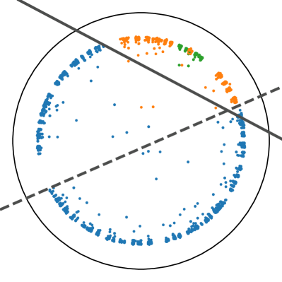
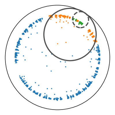
(a)	(b)

Figure 1: Motivation for hyperbolic random forests. The two splits of (a) an oblique Euclidean and (b) a hyperbolic decision tree of depth two with the highest information gain. The data is a tree embedded in hyperbolic space, split into three nested classes. The inductive biases of linear decision boundaries are not appropriate for the underlying geometry.

Current hyperbolic classification algorithms, such as hyperbolic support vector machines (Fan, Yang, and Vemuri 2023) or hyperbolic logistic regression (Ganea, Bécigneul, and Hofmann 2018b) have shown promising results, but still struggle with complex datasets. In Euclidean space, there is a long history of success of tree-based random forest algorithms in this regard (Caruana and Niculescu-Mizil 2006; Fernández-Delgado et al. 2014). We argue that decision trees and, by extension, random forests are well-suited for hyperbolic space due to their shared hierarchical structure. However, to the best of our knowledge, no hyperbolic variant of random forests exists to date. We strive to fill this gap.

Figure 1 illustrates the need for a classifier that fits the underlying geometry, and the benefits of a hyperbolic tree-based classifier. Euclidean hyperplane splits (Figure 1(a)) are ineffective at capturing the structure of the data. In contrast, our hyperbolic splits (Figure 1(b)) are more appropriate for the data, where the nested splits clearly show how the smallest, yellow class is a subtree of the larger, green one.

Tree-based algorithms are built by recursively applying a splitting function; hence, in order to generalize the concept of a tree-based classifier to hyperbolic space, we need to define a hyperbolic splitting function. For this purpose, we propose to use horospheres, which share several desirable properties with the hyperplanes used in Euclidean trees. Due to a combinatorial explosion, finding the optimal horosphere by enumeration is computationally intractable. Instead, we employ a binary classifier to find candidate horospheres. In addition, we introduce two extensions that allow us to find good splits in multi-class and imbalanced scenarios: a heuristic to partition the data into hyperclasses and a class-balanced loss function.

We extensively evaluate our approach on two canonical benchmarks from previous works on hyperbolic classification. Additionally, we introduce three new multi-class hierarchical classification experiments. We show that our method is superior to both competing hyperbolic classifiers as well as their Euclidean counterparts in these settings. Summarized, our contributions are (1) a generalization of random forests to hyperbolic space using horospheres, dubbed HoroRF, (2) two extensions to enable effective learning in multi-class and imbalanced settings, and (3) a thorough evaluation of HoroRF, showing its advantage over other methods, both Euclidean and hyperbolic.

Related Work

Hyperbolic machine learning

Machine learning in hyperbolic space has gained traction due to its inherent hierarchical and compact nature. Foundational work showed that for embedding hierarchies in a continuous space, hyperbolic space is superior to Euclidean space, allowing for embeddings with minimal distortion (Nickel and Kiela 2017; Ganea, Bécigneul, and Hofmann 2018a). Empowered by these results, learning with hyperbolic embeddings has recently been successfully used for various problems. Chami et al. (2019) and Liu, Nickel, and Kiela (2019) showed how to generalize graph networks to hyperbolic space, while Tifrea, Bécigneul, and Ganea (2019) showed the potential of hyperbolic word embeddings. In the visual domain, hyperbolic embeddings have been shown to improve image segmentation (Ghadimi Atigh et al. 2022), zero-shot recognition (Liu et al. 2020), image-text representation learning (Desai et al. 2023), and more. Hyperbolic embeddings have also been effective for biology (Klimovskaia et al. 2020) and in recommender systems (Sun et al. 2021a). We refer to recent surveys for a more complete overview (Peng et al. 2021; Yang et al. 2022; Mettes et al. 2023).

For classification specifically, various traditional classifiers such as logistic regression (Ganea, Bécigneul, and Hofmann 2018b), neural networks (Ganea, Bécigneul, and Hofmann 2018b; Shimizu, Mukuta, and Harada 2021; van Spengler, Berkhout, and Mettes 2023), and support vector machines (SVM) (Cho et al. 2019; Fan, Yang, and Vemuri 2023; Fang, Harandi, and Petersson 2021; Weber et al. 2020) now have counterparts in hyperbolic space. In this work, we strive to go beyond single hyperplane/gyroplane decision boundaries per class and bring random forests to hyperbolic space.

Our method is built on the concept of horospheres, which are the level sets of the Busemann function to ideal points. Ideal points have recently found success in many ways, for instance in supervised classification (Ghadimi Atigh, Keller-Ressel, and Mettes 2021) and self-supervised learning (Durrant and Leontidis 2023). Horospheres, in particular, have found applications in dimensionality reduction (Chami et al. 2021), as well as generalizing SVMs (Fan, Yang, and Vemuri 2023) and neural networks (Sonoda, Ishikawa, and Ikeda 2022) to hyperbolic space, but we are the first to use them as building blocks for random forests.

Random Forests

Random Forests remain a popular choice of classifier to this day due to their high performance, speed, and insensitivity to hyperparameters (Grinsztajn, Oyallon, and Varoquaux 2022). In their original paper (Breiman 2001), two versions of random forests were proposed: one with axis-aligned splits based on a single feature and one with oblique splits based on linear combinations of features. While the optimal axis-aligned split can be found by exhaustive search, finding the optimal oblique split is NP-complete (Heath, Kasif, and Salzberg 1993). As a result, many works have developed heuristics to find good oblique splits in a reasonable time.

One line of work makes use of meta-heuristics such as hill climbing (Murthy et al. 1993), simulated annealing (Heath, Kasif, and Salzberg 1993), or genetic algorithms (Cantú-Paz and Kamath 2003). Other approaches train one or more binary classifiers at every node and choose among the resulting hyperplanes to split the data. Examples include using linear discriminant analysis, ridge regression (Menze et al. 2011), or support vector machines (Do et al. 2010). For multi-class cases, typically, heuristics are employed to partition them into two hyperclasses (Katuwal and Suganthan 2018). We follow the binary classifier approach for our hyperbolic random forests, and we introduce a hyperclass heuristic specifically designed for hyperbolic space.

Hyperbolic Random Forests

The Poincaré ball model

We follow the convention from previous works using horospheres (Chami et al. 2021; Fan, Yang, and Vemuri 2023) and hyperbolic machine learning more broadly (Ganea, Bécigneul, and Hofmann 2018b; Khrulkov et al. 2020; Chien et al. 2021; Shimizu, Mukuta, and Harada 2021) and make use of the Poincaré ball model of hyperbolic space. The Poincaré ball model is defined by the metric space $(\mathds{B}^{n}_{c},g^{\mathds{B}}_{c})$ for a given negative curvature $c$, which we set to 1 throughout this work, where

$$\mathds{B}^{n}_{1}=\{\mathbf{x}\in\mathds{R}^{n}:\|\mathbf{x}\|<1\}$$ (1)

with $\|\cdot\|$ the standard Euclidean norm, and

$$g^{\mathds{B}}_{1}(\mathbf{x})=\frac{2}{1-\|\mathbf{x}\|^{2}}\mathbf{I}_{n}.$$ (2)

From here on, we will omit the curvature subscript for clarity. The distance between two points is given by

$$d_{\mathds{B}}(\mathbf{a},\mathbf{b})=\operatorname{arcosh}\left(1+2\frac{\|\mathbf{a}-\mathbf{b}\|^{2}}{(1-\|\mathbf{a}\|^{2})(1-\|\mathbf{b}\|^{2})}\right),$$ (3)

which is the length of the geodesic arc connecting them. Extending geodesics to infinity in one direction leads to a point on the boundary of the Poincaré ball. These points on the boundary are known as ideal points. The set of all ideal points thus lies on the hypersphere $\mathds{S}^{n-1}$, and they can be interpreted as directions in hyperbolic space (Chami et al. 2021).

HoroRF

In order to generalize random forests to hyperbolic space, we require a way to split data points recursively for any number of classes, regardless of the class frequency distribution, into two partitions with low impurity. In Euclidean space, this splitting function outputs hyperplanes to split the data. For hyperbolic random forests, we propose to use horospheres instead, which can be viewed as hyperbolic variants of Euclidean hyperplanes (Chami et al. 2021).

Formalization

Horospheres are the level sets of the Busemann function (Busemann 1955), which calculates the normalized distance to infinity in a given direction. It can be expressed in closed form in the Poincaré model:

$$B_{\mathbf{w}}(x)=\log\frac{\|\mathbf{w}-\mathbf{x}\|^{2}}{1-\|\mathbf{x}\|^{2}}.$$ (4)

As a result, horospheres $\pi_{\mathbf{w},b}$ are parameterized by an ideal point $\mathbf{w}\in\mathds{R}^{n}$, and a distance to that point $b\in\mathds{R}$, which is the radius of the horosphere. Our goal is to find the optimal horosphere $\pi_{\mathbf{w},b}^{\prime}$ that minimizes the impurity of the resulting partitions or, equivalently, maximizes the information gain. Consider a node $S$ with data $\{(\mathbf{x}_{i},y_{i})\}_{i=1}^{N}$ with $\mathbf{x}\in\mathds{B}^{n}$ and $y\in Y$. The optimal horosphere is given by

$$\pi_{\mathbf{w},b}^{\prime}=\operatorname*{arg\,max}_{\pi_{\mathbf{w},b}}(H(S)-I_{in}-I_{out}),$$ (5)

where $H$ is an impurity measure, and $I_{in}$ and $I_{out}$ give the impurity of the set of points inside and outside of the horosphere, respectively:

$$I_{in} =\frac{N_{in}}{N}H(\{x\in S|B_{w}(x)<b\}),$$

$$I_{out} =\frac{N_{out}}{N}H(\{x\in S|B_{w}(x)\geq b\}).$$ (6)

Here, $N_{in}$ and $N_{out}$ denote the number of samples inside and outside the horosphere. Similar to oblique decision trees in Euclidean space, finding the globally optimal horosphere is computationally infeasible. As such, we need to find approximate solutions.

Finding approximate solutions

Akin to many works on oblique decision trees (e.g., Do et al. (2010); Menze et al. (2011); Katuwal, Suganthan, and Zhang (2020)), we employ a binary classifier at every node to find candidate solutions.

For this, we build upon HoroSVM (Fan, Yang, and Vemuri 2023). HoroSVM uses horospheres to create a large-margin classifier for hyperbolic space. For a labeled dataset $D=\{(\mathbf{x}_{i},y_{i})\}_{i=1}^{N}$ with $\mathbf{x}_{i}\in\mathds{B}^{n}$ and $y_{i}\in\{-1,1\}$, it optimizes the convex loss function

$$\boldsymbol{\ell}(\mu,w,o;D)=\frac{1}{2}\mu^{2}+$$

$$C\sum^{N}_{i=1}\max \left(0,1-y_{i}(\mu(B_{w}^{-1}(\mathbf{x}_{i}))-o)\right),$$ (7)

where

$$B_{\mathbf{w}}^{-1}(\mathbf{x})=\log\frac{1-\|\mathbf{x}\|^{2}}{\|\mathbf{w}-\mathbf{x}\|^{2}},$$ (8)

with $\mu,o\in\mathds{R}^{+}$ and $w\in\mathds{S}^{n-1}$. The slack hyperparameter C controls the trade-off between misclassification tolerance and margin size. Solving for HoroSVM thus results in the three parameters $\mu,\mathbf{w}$, and $o$. In order to transform these results into a horosphere $\pi_{\mathbf{w},b}$, we set $b=-\frac{o}{\mu}$ and use $\mathbf{w}$ directly.

We repeat the classification $K$ times in a one-versus-rest setting, with $K$ the number of classes, and compute the information gain for all resulting horospheres. We select the horosphere with the highest information gain to split the data. We refer to this splitting procedure as the HoroSplitter. While this base version of the HoroSplitter already achieves competitive results, it struggles with imbalanced data, and the one-versus-rest set-up limits its effectiveness in multi-class settings. For that reason, we introduce two additional components to the HoroSplitter that make it more appropriate specifically as a building block for hyperbolic decision trees.

Combining classes

The default HoroSplitter uses a one-versus-rest approach to deal with multi-class data. As a result, it can only find one-versus-rest splits. Nonetheless, a horosphere split with a high information gain could have more than a single class in either partition. To be able to find good splits with multiple classes while avoiding searching over all possible combinations, only the most promising combinations should be evaluated. For this, we design a heuristic that transforms the multi-class problem into a hierarchical set of binary problems by iteratively grouping classes together into two hyperclasses based on their lowest common ancestor (LCA). Then, these binary combinations are added to the pool of one-versus-rest experiments and evaluated for their information gain.

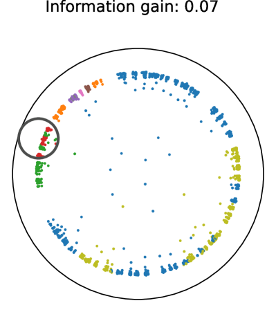
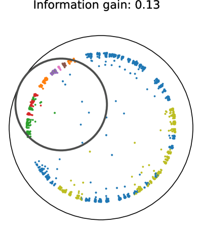
(a)	(b)

Figure 2: Information gain from hierarchical splits. The best (a) one-versus-rest split and (b) split found with our hyperclass heuristic. By considering splits where more than one class is seen as positive, we find splits with a higher information gain.

Recall the connection of hyperbolic space to graph-theoretical trees. In a tree, similar leaf nodes lie in a small subtree and have their LCA at a high depth. In contrast, dissimilar nodes will have their LCA close to the root of the tree. We exploit the analog of this property in hyperbolic space to cluster together the most similar classes first, as similar classes are likely to be capturable by a single horosphere.

We represent each cluster by its hyperbolic mean. As computing the average in the Poincaré model involves the computationally expensive Fréchet mean (Lou et al. 2020), we instead use the Einstein midpoint after transforming the data to Klein coordinates. Specifically, data is transformed into Klein space $\mathds{K}$ with

$$\mathbf{x}_{\mathds{K}}=\frac{2\mathbf{x}_{\mathds{B}}}{1+\|\mathbf{x}_{\mathds{B}}\|^{2}},$$ (9)

and we compute the average $\mathbf{\boldsymbol{\phi}}_{y}$ for class $y$ using

$$\mathbf{\boldsymbol{\phi}}_{y}=\frac{\sum_{i=1}^{N}\mathds{1}_{[y_{i}=y]}\gamma_{i}\mathbf{x}_{i}}{\sum_{i=1}^{N}\gamma_{i}},$$ (10)

where $\gamma_{i}=\frac{1}{\sqrt{1-\|\mathbf{x}_{i}\|^{2}}}$. Afterward, the mean is transformed back to the Poincaré ball with

$$\mathbf{x}_{\mathds{B}}=\frac{\mathbf{x}_{\mathds{K}}}{1+\sqrt{1-\|\mathbf{x}_{\mathds{K}}\|^{2}}}.$$ (11)

We compute all similarities in a pairwise manner and iteratively group the two most similar classes together, where the similarity is based on the LCA of the means of the two classes. The LCA for two points in hyperbolic space is the point that is closest to the origin on the geodesic between them (Chami et al. 2020). As a result, the distance of the LCA from the origin can be seen as a similarity measure. Given two means $\mathbf{\boldsymbol{\phi}}_{i}$ and $\mathbf{\boldsymbol{\phi}}_{j}$, we can calculate their similarity by

$$\textrm{sim}(\mathbf{\boldsymbol{\phi}}_{i},\mathbf{\boldsymbol{\phi}}_{j})=2\tanh^{-1}\left(\sqrt{R^{2}+1}-R\right)$$ (12)

with

$$R=\sqrt{\left(\frac{\|\mathbf{\boldsymbol{\phi}}_{i}\|^{2}+1}{2\|\mathbf{\boldsymbol{\phi}}_{i}\|\cos(\alpha)}\right)^{2}-1}$$ (13)

and

$$\alpha=\tan^{-1}\left(\frac{1}{\sin(\theta)}\left(\frac{\|\mathbf{\boldsymbol{\phi}}_{i}\|(\|\mathbf{\boldsymbol{\phi}}_{j}\|^{2}+1)}{\|\mathbf{\boldsymbol{\phi}}_{j}\|(\|\mathbf{\boldsymbol{\phi}}_{i}\|^{2}+1)}-\cos(\theta)\right)\right),$$ (14)

where $\theta$ is the angle between $\mathbf{\boldsymbol{\phi}}_{i}$ and $\mathbf{\boldsymbol{\phi}}_{j}$. We repeat this until only two hyperclasses are left, for $K-2$ iterations total. As a result, we only evaluate $K+K-2$ horospheres per node. We show an example where evaluating hyperclasses is beneficial in Fig. 2.

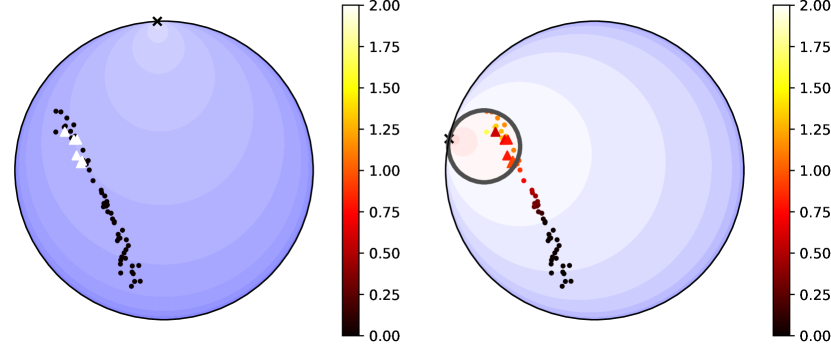
Figure 3: Importance of class balancing. The optimal solution on a binary classification problem found (left) without and (right) with class-balancing. The left horosphere has a large negative $\mathbf{b}$ and does not split the data. In contrast, the right horosphere has a higher loss but a positive information gain. Class labels are given by marker shape, the ideal point given by the x. The points and color bar are colored by loss; the background is colored by distance to the horosphere.

Imbalanced data

SVM-based methods are known to behave poorly on imbalanced data, and HoroSplitter is no exception. We address this by proposing a class-balanced version of the HoroSplitter. Specifically, the problem comes from Eq. (Finding approximate solutions) finding an optimal solution that does not split the data and has an information gain of zero as a result. As an example, consider the binary problem in Figure 3. The optimal horosphere has its ideal point on the top of the Poincaré ball, a $\mu$ very close to 0 and $o$ very close to 1. From Eq. (Finding approximate solutions), it follows that the loss almost reduces to

$$\boldsymbol{\ell}_{\textrm{imbalanced}}(\mu,w,o;D)\approxeq C\sum^{N}_{i=1}\max(0,1+y_{i}),$$ (15)

i.e., approximately 0 for all samples of the negative class and approximately 2 for all samples of the positive class. Thus, in cases where the negative class greatly outnumbers the positive class, the optimal solution finds a very small horosphere for which samples from the positive class get a slightly less confident prediction to be the negative class than samples from the negative class.

We remedy this limitation by incorporating class-balancing into HoroSplitter’s loss function (Cui et al. 2019). We rewrite the loss function in Eq. (Finding approximate solutions) as

$$\boldsymbol{\ell}(\mu,w,o;D)=\frac{1}{2}\mu^{2}+$$ (16)

$$C\sum^{N}_{i=1}\frac{1-\beta}{1-\beta^{n_{y}}} \max(0,1-y_{i}(\mu(B_{w}^{-1}(\mathbf{x}_{i}))-o)),$$

where $n_{y}$ gives the number of training samples belonging to $y$ and $\beta$ is a hyperparameter. By adding more emphasis on the loss for samples of the minority class, we are able to find horospheres that split the data even in imbalanced cases.

Training and inference

We build horospherical decision trees (HoroDT) by repeated application of the HoroSplitter. This process is repeated until all nodes are pure, i.e. contain one class, or a stopping criterion is met. Example stopping criteria include stopping when a node reaches a certain number of samples or no split with an information gain higher than a threshold can be found. By combining multiple HoroDTs into an ensemble, we form a horospherical Random Forest (HoroRF). Each tree is trained on a randomly sampled (with replacement) subset of the data, and a subsample of the features is considered at every split. Predictions are made by a majority vote among the HoroDTs.

Experiments

	Binary		Multi-class
	Karate	Polbooks	Football	Polblogs
Euclidean
LinSVM	95.4$\pm$2.3	92.4$\pm$0.3	33.2$\pm$5.1	85.5$\pm$0.9
RBFSVM	95.4$\pm$2.3	92.4$\pm$0.3	35.5$\pm$4.7	84.4$\pm$1.9
RF	94.3$\pm$3.1	92.1$\pm$0.3	36.2$\pm$4.9	85.1$\pm$2.1
OblRF	94.8 $\pm$2.2	92.1 $\pm$0.3	36.7 $\pm$2.7	84.4 $\pm$1.3
Hyperbolic
HypMLR	93.1$\pm 3.4$	90.9$\pm 0.7$	40.2$\pm 2.5$	81.5$\pm 1.5$
HoroSVM	95.4$\pm$2.3	92.4$\pm$0.2	34.3$\pm$1.8	85.3$\pm$0.8
HoroRF	95.4$\pm$2.3	92.5$\pm$0.3	38.3$\pm$1.8	86.1$\pm$1.0

Table 1: Comparative evaluation on network datasets. We report the mean and standard deviation of the micro-f1 score over five trials of 5-fold stratified cross-validation on four datasets. Underlined gives the best hyperbolic method, Bold denotes the best method overall. HoroRF obtains the best performance on aggregate over the datasets.

	Animal	Group	Worker	Mammal	Tree	Solid	Occupation	Rodent
Euclidean
LinSVM	2.5$\pm 0.0$	6.0$\pm 0.6$	0.7$\pm 0.0$	0.7$\pm 0.0$	0.6$\pm 0.0$	0.8$\pm 0.0$	0.2$\pm 0.0$	0.1$\pm 0.0$
RBFSVM	2.5$\pm 0.0$	6.0$\pm 0.6$	0.7$\pm 0.0$	0.7$\pm 0.0$	0.6$\pm 0.0$	0.8$\pm 0.0$	0.2$\pm 0.0$	0.1$\pm 0.0$
RF	98.6$\pm$0.2	96.6$\pm$0.4	70.0$\pm 3.1$	99.3$\pm$0.3	75.8$\pm 2.0$	92.5$\pm$ 1.2	59.8$\pm 1.1$	34.5$\pm 3.0$
OblRF	98.4$\pm$0.1	96.7 $\pm$0.3	73.3$\pm$1.3	98.8$\pm$0.3	76.2$\pm$3.2	92.9$\pm$1.7	65.0$\pm$2.4	38.2$\pm$0.9
Hyperbolic
HypMLR	3.2 $\pm$0.1	6.5 $\pm$0.0	1.2 $\pm$0.2	0.9 $\pm$0.0	1.3$\pm$0.8	1.0 $\pm$0.2	0.9$\pm$0.9	0.4 $\pm$0.4
HoroSVM	92.4$\pm 1.3$	71.0$\pm 0.5$	39.9$\pm 3.6$	89.8$\pm 0.9$	41.5$\pm 1.0$	65.7$\pm 0.9$	13.0$\pm 1.5$	13.6$\pm 2.0$
HoroRF	98.5$\pm$0.2	96.6$\pm$0.4	73.4$\pm$ 1.7	99.3$\pm$0.4	76.6$\pm$ 3.8	93.5$\pm$ 1.3	65.6$\pm$ 1.5	39.0$\pm$ 2.4

Table 2: Comparative evaluation on binary WordNet experiments. We report the mean and standard deviation of the AUPR on eight experiments averaged over three runs. Underlined gives the best hyperbolic method, Bold denotes the best method overall. On aggregate across the experiments, HoroRF obtains the best performance.

Datasets & Evaluation

We evaluate HoroRF on two canonical hyperbolic classification benchmarks: network node classification and WordNet subtree classification (Cho et al. 2019; Fan, Yang, and Vemuri 2023). Additionally, we introduce three new multi-class WordNet experiments.

Networks

We run node classification experiments on four real-world network datasets embedded into hyperbolic space: karate (34 nodes, 2 classes; Zachary (1977)), polblogs (1224 nodes, 2 classes; Adamic and Glance (2005)), football (115 nodes, 12 classes; Girvan and Newman (2002)), and polbooks (105 nodes, 3 classes).

We use the public embeddings provided by Cho et al. (2019). For each dataset, there are five sets of embeddings; each obtained using the method of Chamberlain, Clough, and Deisenroth (2017). Following previous work (Fan, Yang, and Vemuri 2023), we run a grid search with 5-fold stratified cross-validation and report the best average micro-f1 score over five seeds, where a different embedding is used for each seed.

WordNet

We run binary classification experiments on the nouns of WordNet (Fellbaum 2010), embedded into hyperbolic space using hyperbolic entailment cones (Ganea, Bécigneul, and Hofmann 2018a). The goal is to identify whether a sample belongs to a semantic category (i.e., a subtree of the hyperbolic embeddings). Following (Fan, Yang, and Vemuri 2023), we split the data into 80% for training and 20% for testing and report the results over three runs in AUPR. We find that three of the larger subtrees typically used for these experiments (animal.n.01, group.n.01, mammal.n.01) can be solved near-perfectly with random forests, both Euclidean and hyperbolic. For that reason, we add experiments on two additional subtrees, occupation.n.01 and rodent.n.01, which are smaller than the subtrees evaluated in this type of experiment so far.

Multi-class WordNet

We propose three new multi-class WordNet experiments aimed at evaluating three distinct qualities. In the first experiment, the task is to classify samples into one of multiple subtrees that have the same parent. In the second experiment, we pick nested subtrees, and samples have to be classified into the smallest subtree they belong to. The third experiment combines the two previous experiments with nested classes of multiple subtrees. Unlike previous benchmarks, these are difficult multi-class experiments on large, imbalanced datasets. We provide the full details of the experiments in the appendix.

The datasets are split into train, validation, and test sets with a ratio of 60:20:20. A hyperparameter search is done on the validation set, and the macro-f1 score over three trials on the test set is reported.

	Same	Nested	Both
	level
Euclidean
LinSVM	48.8 $\pm$0.9	59.7 $\pm$0.5	35.6 $\pm$0.2
RBFSVM	80.0 $\pm$1.8	89.8 $\pm$1.1	70.8 $\pm$0.6
RF	89.7$\pm$0.7	91.7$\pm$0.3	81.5$\pm$1.5
OblRF	91.3$\pm$0.6	93.0$\pm$0.2	81.3$\pm$1.4
Hyperbolic
HypMLR	29.0 $\pm$4.5	57.6 $\pm$0.5	35.9 $\pm$6.7
HoroSVM	50.2 $\pm$2.2	56.0 $\pm$0.7	35.2 $\pm$0.5
HoroRF	91.3$\pm$0.3	93.3$\pm$1.1	81.9$\pm$1.5

Table 3: Comparative evaluation on multi-class WordNet. We report results over three trials in macro-f1 score on three experiments. Underlined gives the best hyperbolic method, Bold denotes the best method overall. HoroRF performs best in all settings.

Baselines

We evaluate HoroRF against six baselines, split into two sets. The first set covers hyperbolic classifier baselines, namely hyperbolic multiple logistic regression (HypMLR; Ganea, Bécigneul, and Hofmann (2018b)) and the state-of-the-art hyperbolic SVM, HoroSVM (Fan, Yang, and Vemuri 2023). The second set of baselines comprises Euclidean counterparts of the hyperbolic classifiers, namely a linear SVM (LinSVM), an SVM with an RBF kernel (RBFSVM; (Cortes and Vapnik 1995)), an axis-aligned random forest (RF) (Breiman 2001), and an oblique random forest (OblRF) with a similar set-up to HoroRF. The OblRF uses a cost-balanced linear SVM to find optimal splits (see e.g. (Do et al. 2010)). If the SVM fails to converge, it defaults to using the best axis-aligned split. It finds hyperclasses by iteratively merging the two classes with the closest means.

As is common practice (Cho et al. 2019; Fan, Yang, and Vemuri 2023), the Euclidean baselines are run on the same hyperbolic embeddings as the hyperbolic methods, which we find to perform better compared to mapping the embeddings back to Euclidean space first. Moreover, as the SVMs, HypMLR, and HoroSVM baselines are negatively affected by the class imbalance in the WordNet experiments, we report cost-balanced results on those benchmarks, where the loss is weighted inversely proportional to the class frequency.

Implementation Details

We use 100 trees for HoroRF and all other tree-based methods. We use the Gini impurity to calculate the information gain. At every node, we set $C$ to $2^{n}$ where $n$ is randomly sampled from $\{-3,-2,\ldots,5\}$. We stop splitting when a node reaches a certain number of samples $m$. In the case of ties in information gain between possible splits, a random split is selected. If the HoroSplitter fails to converge, we choose the best horosphere from a small number of random ideal points. We set $m$ and the class-balancing hyperparameter $\beta$ via grid search. Further details are given in the appendix.

Results

Ideal	Hyper-	Class-	f1
Points	classes	balanced
Axis-aligned	✗	✗	9.9
HoroSplitter	✗	✗	35.7
HoroSplitter	✗	✓	36.5
HoroSplitter	✓	✗	37.4
HoroSplitter	✓	✓	38.3

Table 4: Ablating the HoroSplitter in HoroRF on the football dataset. Scores are the micro-f1 score on five times 5-fold stratified cross-validation. Our splitting function, hyperclass-based aggregation, and class balancing are all important for effective hyperbolic random forests.

Networks

The results on the network datasets are shown in Table 1. Our HoroRF outperforms the Euclidean methods in all cases, besides matching the SVMs on karate, showing that the choice of horospheres over hyperplanes results in better performance on data lying in hyperbolic space.

As for the hyperbolic methods, HypMLR is outclassed by both HoroRF and HoroSVM in all cases except football. HoroSVM and HoroRF perform similarly in the binary experiments, with a slight edge for HoroRF on polblogs. In contrast, for the multi-class experiments football and polbooks, HoroRF outclasses HoroSVM by 4.0 and 0.6, respectively, confirming the benefit of HoroRF over HoroSVM in more complex cases.

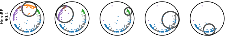
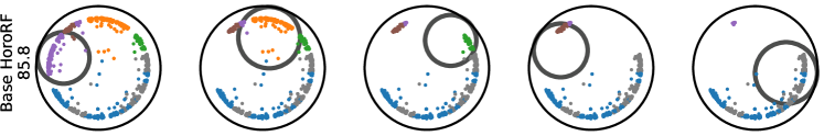
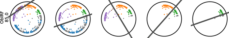
Figure 4: Visualizing HoroRF splits. We show five levels of splits for HoroRF, a base HoroRF without class-balancing and hyperclasses, and OblRF. The dataset is a tree embedded in hyperbolic space, grouped into five classes from two different depths. At every level, the split with the highest impurity is chosen for the visualization of the next level. The performance in macro-f1 is given below the names. All forests consist of one tree and have a maximum depth of six. Splitting in hyperbolic space with balanced and multi-level horospheres obtains the best scores for hierarchical classification data.

WordNet

The results for the WordNet subtree classification experiments are shown in Tab. 2. The Euclidean SVMs are unable to handle the large imbalance in the datasets, despite the loss re-weighting, unlike the tree-based methods. Nonetheless, the results show that HoroRF outperforms the Euclidean tree-based methods in most cases. The differences are most pronounced in the hardest experiments, occupation and rodent, while on the saturated experiments with close to perfect scores, i.e. animal, group, and mammal, we find the tree-based methods to perform similarly.

Similar to the Euclidean SVMs and HypMLR, HoroSVM struggles with the imbalanced data, despite the loss re-weighting, and is not able to approach the performance of HoroRF. We argue this is because real-world data cannot be distinguished with a single horosphere, but requires recursive horospherical separation as done in HoroRF.

Multi-class WordNet

The results for the multi-class WordNet experiments are shown in Table 3, which paint a similar picture as the previous benchmarks. For the Euclidean methods, the tree-based methods outperform the SVMs, with OblRF on average having a slight edge over the axis-aligned random forest. HoroRF outperforms the SVMs and axis-aligned RF in all three cases, and despite reaching an equal score on the first experiment, it is able to outperform OblRF in the remaining two. Compared to the other hyperbolic classifiers, HoroRF is able to reach a far higher performance on these complex imbalanced multi-class experiments, on which both HypMLR and HoroSVM struggle greatly. In conclusion, HoroRF is the most consistent and best-performing classifier across all benchmarks.

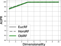
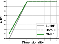
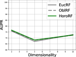
(a)	(b)	(c)

Figure 5: Effect of embedding dimensionality. Performance of HoroRF and OblRF in AUPR on 2, 5, and 10-dimensional WordNet embeddings for the (a) solid, (b) occupation, and (c) tree subtrees.

Ablations and visualizations

Ablating hyperclasses and balancing.

We perform an ablation study to validate our choices on the football dataset. From Tab. 4, we find there is a large benefit in using our HoroSplitter to find splits, as opposed to enumerating all possible horospheres at axis-aligned ideal points. Furthermore, we show how both our hyperclass and class-balancing additions improve upon the base HoroSplitter, and their combination enables us to reach the best performance.

Visualizing splits

In Fig. 6, we show how HoroRF, HoroRF without additions, and OblRF find splits on a 5-way classification task. HoroRF reaches the highest performance due to its hyperclass-based splitting, unlike HoroRF without additions, and by using splits appropriate for the underlying geometry, unlike OblRF.

Higher dimensional embeddings

We show how the performance of HoroRF is affected by increasing the dimensionality of the WordNet embeddings in Fig. 5. For most cases, increasing the dimensionality leads to a trivial problem with a near-perfect AUPR. An exception is tree, where the AUPR on both the 5-dimensional and 10-dimensional embeddings is lower than on the 2-dimensional one. We find that RF and OblRF also suffer in this setting, highlighting limitations in the embeddings themselves.

Conclusion

We presented HoroRF, a random forest algorithm in hyperbolic space. Its trees are constructed by repeated application of the HoroSplitter, which finds horosphere-based splits with high information gain. We show the benefits of additional components aimed at improving performance on imbalanced and multi-class datasets. Extensive experiments on two established and one newly introduced benchmark show its superiority over both existing hyperbolic classifiers as well as their Euclidean counterparts. Further advances in hyperbolic classification can easily be incorporated into the framework, as HoroRF is in no way restricted to a single type of classifier. In future work, we aim to investigate the benefits of combining multiple types of splits, for example by including hyperbolic logistic regression to provide additional splits to include next to the horosphere splits.

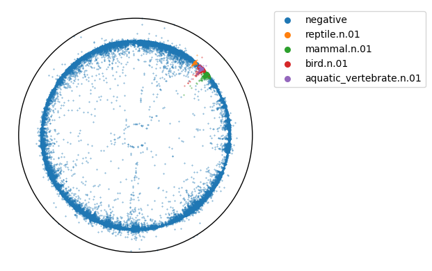
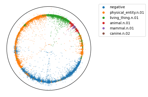
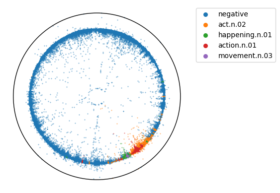
(a)	(b)	(c)

Figure 6: Visualizing the multi-class WordNet experiments. We embed all WordNet nouns into two dimensions with hyperbolic entailment cones (Ganea, Bécigneul, and Hofmann 2018a) and color the different classes of our three multi-class WordNet experiments.

Appendix A Supplementary Material

Multi-class WordNet details

For the first experiment, we take four subtrees of the vertebrate.n.01 subtree: reptile.n.01, mammal.n.01, bird.n.01, and aquatic_vertebrate.n.01. Together with the negative class, this leads to a 5-way classification problem.

For the second experiment, we take nested subtrees: physical_entity.n.01: living_thing.n.01, animal.n.01, mammal.n.01, and canine.n.01. Together with the negative class, this leads to a 6-way classification problem.

For the third experiment, we combine the two. We take the act.n.01 subtree, as well as its subtree happening.n.01. Additionally, we include action.n.01 and its subtree movement.n.03. Together with the negative class, this leads to a 5-way classification problem. Visualizations in 2D for the three experiments are given in Fig. 6.

Full implementation details

We run a grid search for all methods. For the linear SVM, we search over $C\in\{-5,-4,\cdots,15\}$. For the RBF SVM, we search over $C\in\{-5,-1,\cdots,15\}$ and $\gamma\in\{-15,-11,\cdots,1,3\}$. For the random forest and oblique random forest, we search over the hyperparameter that controls at what number of samples to stop splitting a node $m\in\{1,3,5\}$ on the small network datasets and $m\in\{3,7,11\}$ on the larger WordNet datasets. For the hyperbolic logistic regression, we search over the learning rate $lr\in\{0.1,0.01,0.001\}$, and the batch size $bs\in\{16,32,64\}$ on the network datasets and $bs\in\{128,256,512\}$ on the WordNet datasets. For HoroSVM, we search over $C\in\{-5,-4,\cdots,15\}$. For HoroRF, we search over $\beta\in\{0,0.9,\cdots,0.9999\}$, and $m\in\{1,3,5\}$ on the network datasets and $m\in\{3,7,11\}$ on the WordNet datasets.

We run all our experiments on a machine running CentOS 7.9.2009 with an AMD EPYC 7302 16-Core Processor with access to 48GB of memory. We set our seeds such that our implementation of the HoroSVM baseline resembles the results on the network datasets reported in its original publication.

References

- Adamic and Glance (2005) Adamic, L. A.; and Glance, N. 2005. The political blogosphere and the 2004 US election: divided they blog. In Proceedings of the 3rd international workshop on Link discovery, 36–43.
- Ahmad and Lecue (2022) Ahmad, O.; and Lecue, F. 2022. FisheyeHDK: Hyperbolic deformable kernel learning for ultra-wide field-of-view image recognition. In Proceedings of the AAAI Conference on Artificial Intelligence, volume 36, 5968–5975.
- Breiman (2001) Breiman, L. 2001. Random forests. Machine learning, 45: 5–32.
- Busemann (1955) Busemann, H. 1955. The geometry of geodesics. Academic Press.
- Cantú-Paz and Kamath (2003) Cantú-Paz, E.; and Kamath, C. 2003. Inducing oblique decision trees with evolutionary algorithms. IEEE Transactions on Evolutionary Computation, 7(1): 54–68.
- Caruana and Niculescu-Mizil (2006) Caruana, R.; and Niculescu-Mizil, A. 2006. An empirical comparison of supervised learning algorithms. In Proceedings of the 23rd international conference on Machine learning, 161–168.
- Chamberlain, Clough, and Deisenroth (2017) Chamberlain, B. P.; Clough, J.; and Deisenroth, M. P. 2017. Neural embeddings of graphs in hyperbolic space. arXiv preprint arXiv:1705.10359.
- Chami et al. (2020) Chami, I.; Gu, A.; Chatziafratis, V.; and Ré, C. 2020. From trees to continuous embeddings and back: Hyperbolic hierarchical clustering. Advances in Neural Information Processing Systems, 33: 15065–15076.
- Chami et al. (2021) Chami, I.; Gu, A.; Nguyen, D. P.; and Ré, C. 2021. Horopca: Hyperbolic dimensionality reduction via horospherical projections. In International Conference on Machine Learning, 1419–1429. PMLR.
- Chami et al. (2019) Chami, I.; Ying, Z.; Ré, C.; and Leskovec, J. 2019. Hyperbolic graph convolutional neural networks. Advances in neural information processing systems.
- Chien et al. (2021) Chien, E.; Pan, C.; Tabaghi, P.; and Milenkovic, O. 2021. Highly scalable and provably accurate classification in poincaré balls. In 2021 IEEE International Conference on Data Mining (ICDM), 61–70. IEEE.
- Cho et al. (2019) Cho, H.; DeMeo, B.; Peng, J.; and Berger, B. 2019. Large-margin classification in hyperbolic space. In The 22nd international conference on artificial intelligence and statistics, 1832–1840. PMLR.
- Cortes and Vapnik (1995) Cortes, C.; and Vapnik, V. 1995. Support-vector networks. Machine learning, 20: 273–297.
- Cui et al. (2019) Cui, Y.; Jia, M.; Lin, T.-Y.; Song, Y.; and Belongie, S. 2019. Class-balanced loss based on effective number of samples. In Proceedings of the IEEE/CVF conference on computer vision and pattern recognition, 9268–9277.
- Desai et al. (2023) Desai, K.; Nickel, M.; Rajpurohit, T.; Johnson, J.; and Vedantam, S. R. 2023. Hyperbolic image-text representations. In International Conference on Machine Learning.
- Do et al. (2010) Do, T.-N.; Lenca, P.; Lallich, S.; and Pham, N.-K. 2010. Classifying very-high-dimensional data with random forests of oblique decision trees. Advances in knowledge discovery and management, 39–55.
- Durrant and Leontidis (2023) Durrant, A.; and Leontidis, G. 2023. HMSN: Hyperbolic Self-Supervised Learning by Clustering with Ideal Prototypes. arXiv preprint arXiv:2305.10926.
- Fan, Yang, and Vemuri (2023) Fan, X.; Yang, C.-H.; and Vemuri, B. C. 2023. Horocycle Decision Boundaries for Large Margin Classification in Hyperbolic Space. arXiv preprint arXiv:2302.06807.
- Fang, Harandi, and Petersson (2021) Fang, P.; Harandi, M.; and Petersson, L. 2021. Kernel methods in hyperbolic spaces. In Proceedings of the IEEE/CVF International Conference on Computer Vision, 10665–10674.
- Fellbaum (2010) Fellbaum, C. 2010. Princeton university: About wordnet.
- Fernández-Delgado et al. (2014) Fernández-Delgado, M.; Cernadas, E.; Barro, S.; and Amorim, D. 2014. Do we need hundreds of classifiers to solve real world classification problems? The journal of machine learning research, 15(1): 3133–3181.
- Ganea, Bécigneul, and Hofmann (2018a) Ganea, O.; Bécigneul, G.; and Hofmann, T. 2018a. Hyperbolic entailment cones for learning hierarchical embeddings. In International Conference on Machine Learning, 1646–1655. PMLR.
- Ganea, Bécigneul, and Hofmann (2018b) Ganea, O.; Bécigneul, G.; and Hofmann, T. 2018b. Hyperbolic neural networks. Advances in neural information processing systems, 31.
- Ghadimi Atigh, Keller-Ressel, and Mettes (2021) Ghadimi Atigh, M.; Keller-Ressel, M.; and Mettes, P. 2021. Hyperbolic Busemann Learning with Ideal Prototypes. Advances in Neural Information Processing Systems, 34: 103–115.
- Ghadimi Atigh et al. (2022) Ghadimi Atigh, M.; Schoep, J.; Acar, E.; Van Noord, N.; and Mettes, P. 2022. Hyperbolic image segmentation. In Proceedings of the IEEE/CVF conference on computer vision and pattern recognition.
- Girvan and Newman (2002) Girvan, M.; and Newman, M. E. 2002. Community structure in social and biological networks. Proceedings of the national academy of sciences, 99(12): 7821–7826.
- Grinsztajn, Oyallon, and Varoquaux (2022) Grinsztajn, L.; Oyallon, E.; and Varoquaux, G. 2022. Why do tree-based models still outperform deep learning on typical tabular data? Advances in Neural Information Processing Systems, 35: 507–520.
- Heath, Kasif, and Salzberg (1993) Heath, D.; Kasif, S.; and Salzberg, S. 1993. Induction of oblique decision trees. In IJCAI, volume 1993, 1002–1007. Citeseer.
- Katuwal and Suganthan (2018) Katuwal, R.; and Suganthan, P. N. 2018. Enhancing multi-class classification of random forest using random vector functional neural network and oblique decision surfaces. In 2018 International Joint Conference on Neural Networks, 1–8. IEEE.
- Katuwal, Suganthan, and Zhang (2020) Katuwal, R.; Suganthan, P. N.; and Zhang, L. 2020. Heterogeneous oblique random forest. Pattern Recognition, 99: 107078.
- Khrulkov et al. (2020) Khrulkov, V.; Mirvakhabova, L.; Ustinova, E.; Oseledets, I.; and Lempitsky, V. 2020. Hyperbolic image embeddings. In Proceedings of the IEEE/CVF Conference on Computer Vision and Pattern Recognition, 6418–6428.
- Klimovskaia et al. (2020) Klimovskaia, A.; Lopez-Paz, D.; Bottou, L.; and Nickel, M. 2020. Poincaré maps for analyzing complex hierarchies in single-cell data. Nature communications, 11(1): 2966.
- Liu, Nickel, and Kiela (2019) Liu, Q.; Nickel, M.; and Kiela, D. 2019. Hyperbolic graph neural networks. Advances in neural information processing systems.
- Liu et al. (2020) Liu, S.; Chen, J.; Pan, L.; Ngo, C.-W.; Chua, T.-S.; and Jiang, Y.-G. 2020. Hyperbolic visual embedding learning for zero-shot recognition. In Proceedings of the IEEE/CVF conference on computer vision and pattern recognition.
- Lou et al. (2020) Lou, A.; Katsman, I.; Jiang, Q.; Belongie, S.; Lim, S.-N.; and De Sa, C. 2020. Differentiating through the fréchet mean. In International Conference on Machine Learning.
- Marconi, Ciliberto, and Rosasco (2020) Marconi, G.; Ciliberto, C.; and Rosasco, L. 2020. Hyperbolic manifold regression. In International Conference on Artificial Intelligence and Statistics, 2570–2580. PMLR.
- Menze et al. (2011) Menze, B. H.; Kelm, B. M.; Splitthoff, D. N.; Koethe, U.; and Hamprecht, F. A. 2011. On oblique random forests. In Machine Learning and Knowledge Discovery in Databases: European Conference, ECML PKDD 2011, Athens, Greece, September 5-9, 2011, Proceedings, Part II 22, 453–469. Springer.
- Mettes et al. (2023) Mettes, P.; Atigh, M. G.; Keller-Ressel, M.; Gu, J.; and Yeung, S. 2023. Hyperbolic Deep Learning in Computer Vision: A Survey. arXiv preprint arXiv:2305.06611.
- Monath et al. (2019) Monath, N.; Zaheer, M.; Silva, D.; McCallum, A.; and Ahmed, A. 2019. Gradient-based hierarchical clustering using continuous representations of trees in hyperbolic space. In Proceedings of the 25th ACM SIGKDD International Conference on Knowledge Discovery & Data Mining, 714–722.
- Murthy et al. (1993) Murthy, S. K.; Kasif, S.; Salzberg, S.; and Beigel, R. 1993. OC1: A randomized algorithm for building oblique decision trees. In Proceedings of AAAI, volume 93, 322–327. Citeseer.
- Nickel and Kiela (2017) Nickel, M.; and Kiela, D. 2017. Poincaré embeddings for learning hierarchical representations. In Advances in neural information processing systems, volume 30.
- Nickel and Kiela (2018) Nickel, M.; and Kiela, D. 2018. Learning continuous hierarchies in the lorentz model of hyperbolic geometry. In International conference on machine learning.
- Pan et al. (2023) Pan, C.; Chien, E.; Tabaghi, P.; Peng, J.; and Milenkovic, O. 2023. Provably accurate and scalable linear classifiers in hyperbolic spaces. Knowledge and Information Systems, 1–34.
- Peng et al. (2021) Peng, W.; Varanka, T.; Mostafa, A.; Shi, H.; and Zhao, G. 2021. Hyperbolic deep neural networks: A survey. IEEE Transactions on pattern analysis and machine intelligence, 44(12): 10023–10044.
- Shimizu, Mukuta, and Harada (2021) Shimizu, R.; Mukuta, Y.; and Harada, T. 2021. Hyperbolic neural networks++. In International Conference on Learning Representations.
- Sonoda, Ishikawa, and Ikeda (2022) Sonoda, S.; Ishikawa, I.; and Ikeda, M. 2022. Fully-Connected Network on Noncompact Symmetric Space and Ridgelet Transform based on Helgason-Fourier Analysis. In International Conference on Machine Learning, 20405–20422. PMLR.
- Sun et al. (2021a) Sun, J.; Cheng, Z.; Zuberi, S.; Pérez, F.; and Volkovs, M. 2021a. Hgcf: Hyperbolic graph convolution networks for collaborative filtering. In Proceedings of the Web Conference 2021.
- Sun et al. (2021b) Sun, L.; Zhang, Z.; Zhang, J.; Wang, F.; Peng, H.; Su, S.; and Philip, S. Y. 2021b. Hyperbolic variational graph neural network for modeling dynamic graphs. In Proceedings of the AAAI Conference on Artificial Intelligence, volume 35, 4375–4383.
- Tai, Li, and Ku (2022) Tai, C.-Y.; Li, M.-Y.; and Ku, L.-W. 2022. Hyperbolic disentangled representation for fine-grained aspect extraction. In Proceedings of the AAAI Conference on Artificial Intelligence, volume 36, 11358–11366.
- Tifrea, Bécigneul, and Ganea (2019) Tifrea, A.; Bécigneul, G.; and Ganea, O.-E. 2019. Poincaré glove: Hyperbolic word embeddings. International Conference on Learning Representations.
- van Spengler, Berkhout, and Mettes (2023) van Spengler, M.; Berkhout, E.; and Mettes, P. 2023. Poincaré ResNet. In International Conference on Computer Vision.
- Weber et al. (2020) Weber, M.; Zaheer, M.; Rawat, A. S.; Menon, A. K.; and Kumar, S. 2020. Robust large-margin learning in hyperbolic space. Advances in Neural Information Processing Systems, 33: 17863–17873.
- Yang et al. (2022) Yang, M.; Zhou, M.; Li, Z.; Liu, J.; Pan, L.; Xiong, H.; and King, I. 2022. Hyperbolic graph neural networks: a review of methods and applications. arXiv preprint arXiv:2202.13852.
- Zachary (1977) Zachary, W. W. 1977. An information flow model for conflict and fission in small groups. Journal of anthropological research, 33(4): 452–473.