Simulating LDPC code Hamiltonians on 2D lattices

Abstract

While LDPC codes have been demonstrated with desirable error correcting properties, this has come at a cost of diverging from the geometrical constraints of many hardware platforms. Viewing codes as the groundspace of a Hamiltonian, we consider engineering a simulation Hamiltonian reproducing some relevant features of the code. Techniques from Hamiltonian simulation theory are used to build a simulation of LDPC codes using only 2D nearest-neighbour interactions at the cost of an energy penalty polynomial in the system size. We derive guarantees for the simulation that allows us to approximately reproduce the ground state of the code Hamiltonian, approximating a $[[N,\Omega(\sqrt{N}),\Omega(\sqrt{N})]]$ code in 2D. The key ingredient is a new constructive tool to simulate an $l$-long interaction between two qubits by a 1D chain of $l$ nearest-neighbour interacting qubits using $\operatorname{\mathrm{poly}}(l)$ interaction strengths. This is an exponential advantage over the existing gadgets for this routine which facilitates the first $\epsilon$-simulation of arbitrary sparse Hamiltonian on $n$ qubits with a Hamiltonian on a 2D lattice of $O(n^{2})$ qubits with interaction strengths scaling as $O\left(\mathrm{poly}(n,1/\epsilon)\right)$.

1 Introduction

As quantum computers are inherently sensitive to noise, quantum codes have become an important primitive in their engineering. However, despite their apparent necessity, they are also expected to incur significant overhead. There is thus a strong interest in understanding the most efficient codes an architecture can operate [1, 2], in the hope of limiting these additional costs. One of the major results from this line of research is that geometrically local architectures can only be so efficient. For example, most codes can be defined as the groundstate of a sparse Hamiltonian $H=\sum_{i}h_{i}$, and if additionally constrained to be a 2D commuting projector Hamiltonian – the case for a large number of codes known and used today – obey $kd^{2}\in O(n),d\in O(\sqrt{n})$ [1, 2]. Here $k$ is the number of logical qubits, $d$ is the distance, and $n$ is the number of physical qubits used in the $[[n,k,d]]$ quantum code.

On the other hand, if the geometrical restriction is dropped, quantum codes can achieve parameters scaling as $[[n,\Theta(n),\Theta(n)]]$ [3, 4]. There thus exists a landscape of parameters $k,d$ between 2D commuting projector Hamiltonians, and sparse Hamiltonians in general. In this work we contribute to the exploration of this landscape by proving that an arbitrary quantum LDPC code can be simulated by a 2D nearest-neighbour Hamiltonian $\tilde{H}=\sum\tilde{h}_{j}$ acting on $O(n^{2})$ qubits, with an interaction strength $\norm{\tilde{h}_{j}}$ that scales polynomially with the system size and the reciprocal of the simulation error.

When codes are expressed as a Hamiltonian groundspace, the computations that run within this subspace will be protected from ambient errors. Errors translate into excitations of the Hamiltonian and measuring these excitations can be used to correct those errors. So naturally, operating a quantum code requires the ability to reliably produce these ground states and hence requires our simulation to not only preserve the eigenspectrum but also the eigenstates. This is in stark contrast with the usual simulation results, which guarantee a small difference in energy eigenvalues between the simulator Hamiltonian and original code Hamiltonian – however, that alone is trivial since all $[[n,k,d]]$ codes are unitarily equivalent.

Our simulation successfully overcomes these limitations, more precisely we show that:

Theorem 21 (Simulating LDPC codes (informal) Theorem 21).

Given a Hamiltonian $H=\sum_{i}h_{i}$ corresponding to an arbitrary LDPC code $\mathcal{C}$ acting on register $\mathcal{H}$ of $n$ qubits . $\exists$ a 2D nearest-neighbour Hamiltonian, $\tilde{H}=\sum_{j}\tilde{h}_{j}$, acting on an augmented register $\mathcal{H}\otimes\mathcal{A}$ of $N\in O(n^{2})$ qubits such that,

1. The interaction strength of $\tilde{H}$ scales as $\operatorname{\mathrm{poly}}(n,\zeta^{-1}))$.

2. States close to the groundstates of $\tilde{H}$ are close to the groundstate of $H$. I.e. If $\rho$ is a low-energy state in $\mathcal{H}\otimes\mathcal{A}$ with $\tr(\rho\tilde{H})\leq E$, then $\tr(\rho_{\mathcal{H}}H)\in O(E+\zeta)$.

3. All ground states of $H$ are close to the groundstates of $\tilde{H}$ given the right ancilla state. I.e. Let $\sigma$ be a state in the support of $\mathcal{S}(\mathcal{H})$ then, $\exists$ $\tilde{\sigma}\in\mathcal{S}(\mathcal{H}\otimes\mathcal{A})$, close to $\sigma$ on the original register $\norm{\tr_{\mathcal{A}}(\tilde{\sigma})-\sigma}_{1}\in O(\zeta)$ where $\absolutevalue{\tr(\tilde{\sigma}\tilde{H})-\tr(\sigma H)}\leq\zeta.$

4. The low-energy eigenspectrum of $\tilde{H}$ $\zeta$-approximates the eigenspectrum of $H$.

for any $\zeta,E\geq 0$ where $\mathcal{S}(\mathcal{H})$ denotes the set of states acting on $\mathcal{H}$.

In error correcting terms, item 2 states that low-energy states of $\tilde{H}$ have a small syndrome with respect to the code Hamiltonian $H$. And conversely, item 3 states that all code states in the ground space of $H$ can be found in the ground space of $\tilde{H}$, up to a small controllable error. Together, those properties show that the low-energy space of $\tilde{H}$ is precisely the low-syndrome space of $H$, up to a small error.

We are free to tune error parameter $\zeta$ to reduce this error at the expense of increasing the interaction strength. Since we use $N\in O(n^{2})$ qubits in total, we effectively simulate a $[[N,\Omega(\sqrt{N}),\Omega(\sqrt{N})]]$ code in 2D. The fact that the groundspace of LDPC codes can be made accessible to 2D architecture is surprising, as they generally require either long-range interactions, or instantaneous classical communications.

The proof of this result heavily relies on tools from the literature on analogue simulation of quantum systems, specifically perturbation gadgets. Emerging from Hamiltonian complexity theory [5], perturbation gadgets are one of a handful of constructive simulation techniques. The gadgets iteratively morph sections of Hamiltonian interaction graphs at the cost of additional qubits. This allows restricted Hamiltonians to emulate the physics of a larger range of more complex systems in the low energy regime. However, the interaction strengths involved to apply multiple rounds of perturbation theory are in general impractical to implement: a $\zeta$-simulation involving $r$ rounds of perturbation on a $n$-qubit Hamiltonian requires strengths of $O\left(\left(\zeta^{-1}\mathrm{poly}(n)\right)^{6^{r}}\right)$. Nevertheless, if the number of rounds of perturbation theory is restricted to $O(1)$ then simulator Hamiltonian weights are ‘only’ polynomially growing with the system size.

LDPC codes are described by general sparse Hamiltonians whereby the degree and locality is bounded by a constant, but when planarised the interaction graph edges can be $O(n)$ long. These long-range interactions are integral for expansion which is closely linked to good error correcting properties. Using existing gadgets fitting these $O(n)$-long range interactions onto a lattice required $O(\log n)$ rounds of perturbation theory and hence $\exp(n)$ interaction strengths. It was unclear whether this energy resource was a necessary requirement for the perturbative simulation. Our main technical contribution is to develop a new gadget that in a single step simulates a 2-qubit interaction with a chain of $n$, 2-qubit interactions using strengths scaling as $O(\mathrm{poly}(n,\zeta^{-1}))$ - an exponential improvement.

History state simulations [6, 7] provide an alternative to perturbative techniques. In these works the target Hamiltonian is encoded into a 1D quantum phase estimation circuit before obtaining the simulator Hamiltonian from the Feynman-Kitaev circuit-to-Hamiltonian construction [8]. [9] recently constructed the first protocol for simulating a general local Hamiltonian with a geometrically local Hamiltonian with polynomial resources using these ideas. The simulator Hamiltonian in this construction acts on $\mathrm{poly}(n,\zeta^{-1})$ qubits and therefore the lattice size depends on the simulation error. While our technique additionally requires the target Hamiltonian to be sparse (each qubit acted on non-trivially by a constant number of Hamiltonian terms), the simulator acts on only $O(n^{2})$ qubits independent of the simulation error so the same lattice can be used while taking the error arbitrarily small. The quadratic ancillas in this work is also a polynomial improvement over the general poly in [9].

This work was motivated by LDPC codes however, the technique provides a general protocol for constructing a 2D lattice simulator Hamiltonian of arbitrary sparse Hamiltonians using only polynomial interaction strengths and quadratically many ancilla qubits. Analogue simulation is an important near-term application of quantum computers hence the broader simulation result is of interest independently of code Hamiltonians.

Corollary 18 (Simulating sparse Hamiltonians (informal)).

Given a Pauli Hamiltonian, $H=\sum_{i}h_{i}$, acting on $n$ qubits that is sparse: $O(1)$-local and the maximum degree is $O(1)$.

$\exists$ a nearest-neighbour Hamiltonian, $\tilde{H}=\sum_{j}\tilde{h}_{j}$, acting on a 2D lattice of $N=O(n^{2})$ qubits, $\tilde{H}=\sum_{j}\tilde{h}_{j}$, that is a simulation of $H$ with interaction strength scaling polynomially in $n$ and inverse polynomially with the precision of the simulation.

1.1 Open questions

The main drawback of our construction is the polynomial interaction strength it incurs. Having $\norm{h_{i}}$ depend solely on $\zeta$ instead would be highly desirable and constitute a natural research question: can the dependence be improved, or is it possible to lower bound $\norm{h_{i}}$? Unfortunately, we show in Appendix B that superficial improvements to our gadget cannot yield this scaling. We first highlight two weakenings of our main result that do not disrupt the application to codes (and remain interesting in an analogue simulation context) but may reduce the required resources:

Open Problem 1.

To what extend can the construction be improved assuming that the target Hamiltonian is commuting and sparse? – as is the case for most codes studied.

Open Problem 2.

To what extend can the construction be improved if we are solely interested in preserving the properties of the ground state?

To exemplify 2 consider the 4-body Hamiltonian $H=Z_{1}Z_{2}Z_{3}Z_{4}$, introduce three ancilla qubits $\mathcal{H}_{a},\mathcal{H}_{b},\mathcal{H}_{c}$, and consider the simulation Hamiltonian $H^{\prime}=Z_{1}Z_{2}Z_{a}+Z_{3}Z_{4}Z_{b}+Z_{a}Z_{b}Z_{c}+Z_{c}$. Then for any state in the ground space of $H^{\prime}$, its restriction on the data qubits is also in the ground space of $H$. Conversely, for any state in the ground space of $H$, there exists a state on the ancilla subsystem such that the state is in the groundspace of $H^{\prime}$.

This example falls outside of known universal simulation methods, and indeed it seems unlikely that simulating even just the groundstate of sparse commuting Hamiltonians could generally be done with constant interaction strength. The argument for this pessimism takes inspiration from Appendix B: consider the target Hamiltonian $H=-ZZ-XX$, which stabilizes $|00\rangle+|11\rangle$. If the two qubits are $\Omega(n)$ far from each other, the correlation between the two qubits has to decay slowly with the distance. It follows from the exponential clustering theorem [10], that the interaction strength $\mu$ of any simulation Hamiltonian with a unique ground state reproducing the ground state of $H$ has to obey $\mu\in\tilde{\Omega}(n)$. Although allowing degeneracy in the ancilla subsystem would circumvent this line of reasoning, the uniqueness is a fundamental resource in current constructions – particularly in the eigenstate correspondence.

We now turn to the question of how this construction could be used to reliably store information. In particular, it is clear that if the target Hamiltonian has an energy barrier, then the simulation Hamiltonian also does. To what extent are other properties preserved?

Open Problem 3.

the target Hamiltonian is quantum memory, does the simulation behave similarly? In general, does this construction preserve topological phases?

Open Problem 4.

Can a decoder for the target Hamiltonian be mapped to a decoder for the simulation Hamiltonian? Can the simulation be used in a fault-tolerant context?

Considering adiabatic computing, our results could be used to simulate arbitrary sparse Hamiltonians on these platforms even when their connectivity is limited. Whether this can be utilised as a practical tool for interesting simulations on near-term hardware remains to be seen. This would require keeping track of error terms explicitly to get a handle of the constants involved in our asymptotic scalings.

Open Problem 5.

Are there any physically relevant sparse Hamiltonians where our protocol newly facilitates a practical simulation implementation on current quantum analogue platforms?

Finally, it might be of independent interest to note that our long-range gadgets provide new proofs of known results, [5]. Indeed since the $k$-local problem on sparse Hamiltonians is QMA-complete [11], our result naturally shows that this hardness extends to 2D spin systems.

2 Hamiltonian simulation

Hamiltonian simulation, as referred to in this work, involves engineering a Hamiltonian that exhibits approximately the same physical properties as a target Hamiltonian, while the structure and features of the two Hamiltonians may be vastly different. This section introduces some definitions and key results from Hamiltonian simulation literature that we will employ in this work.

Formally an approximate simulation is defined as,

Definition 6 (Approximate simulation [12]).

We say that $H_{\textup{sim}}$ is a $(\Delta,\eta,\epsilon)$-simulation of $H_{\textup{target}}$ if there exists a local encoding $\mathcal{E}(M)=T\left(M\otimes P+\overline{M}\otimes Q\right)T^{\dagger}$ such that:

1. There exists an encoding $\tilde{\mathcal{E}}(M)=\tilde{T}\left(M\otimes P+\overline{M}\otimes Q\right)\tilde{T}^{\dagger}$ such that $\tilde{T}\mathds{1}\tilde{T}^{\dagger}$ is the projector into the low ($<\Delta$) energy subspace of $H_{\textup{sim}}$ and $\norm{\tilde{T}-T}_{\infty}\leq\eta$

2. $\norm{(H_{\textup{sim}})_{\leq\Delta}-\tilde{\mathcal{E}}(H_{\textup{target}})}_{\infty}\leq\epsilon$.

An encoding is a map $\mathcal{E}:\textup{Herm}_{n}\mapsto\textup{Herm}_{m}$ of the form: $\tilde{\mathcal{E}}(M)=\tilde{T}\left(M\otimes P+\overline{M}\otimes Q\right)\tilde{T}^{\dagger}$ where $P$, $Q$ are orthogonal complementary projectors ($P+Q=\mathds{1}$), $T$ is an isometry and overline denote complex conjugation.

This definition has three parameters describing the approximation in the simulation. The physics of the target system is encoded in the subspace of $H_{\text{sim}}$ with energy less that $\Delta$, the high energy subspace simulator Hamiltonian contributes inaccuracies to the physics observed hence in good simulations $\Delta$ is taken large to minimise these effects. $\eta$ describes the error in the eigenstates since the local encoding describing the simulation does not map perfectly into the low energy subspace but instead is close to a general encoding that does. Finally $\epsilon$ describes the error in the eigenspectrum, a simple consequence of (ii) is that the low energy spectrum of the simulator is $\epsilon$-close to the spectrum of the target. Given small $\epsilon$ and $\eta$ the eigenspectrum and corresponding states of the target are well approximated by the simulator. In [12] it is shown that approximate simulations preserves important physical quantities up to controllable errors:

Lemma 7 ([12, Lem. 27, Prop. 28, Prop. 29]).

Let $H$ act on $(\mathbb{C}^{d})^{\otimes n}$. Let $H^{\prime}$ act on $(\mathbb{C}^{d^{\prime}})^{\otimes m}$, such that $H^{\prime}$ is a $(\Delta,\eta,\epsilon)$-simulation of $H$ with corresponding local encoding $\mathcal{E}(M)=T(M\otimes P+\overline{M}\otimes Q)T^{\dagger}$. Let $p=\rank(P)$ and $q=\rank(Q)$. Then the following holds true.

1. Denoting with $\lambda_{i}(H)$ (resp. $\lambda_{i}(H^{\prime})$) the $i$^th-smallest eigenvalue of $H$ (resp. $H^{\prime}$), then for all $1\leq i\leq d^{n}$, and all $(i-1)(p+q)\leq j\leq i(p+q)$, $|\lambda_{i}(H)-\lambda_{j}(H^{\prime})|\leq\epsilon$.

2. The relative error in the partition function evaluated at $\beta$ satisfies

   $$\frac{|\mathcal{Z}_{H^{\prime}}(\beta)-(p+q)\mathcal{Z}_{H}(\beta)|}{(p+q)\mathcal{Z}_{H}(\beta)}\leq\frac{(d^{\prime})^{m}\mathrm{e}^{-\beta\Delta}}{(p+q)d^{n}\mathrm{e}^{-\beta\|H\|}}+(\mathrm{e}^{\epsilon\beta}-1).$$

3. For any density matrix $\rho^{\prime}$ in the encoded subspace for which $\mathcal{E}(\mathds{1})\rho^{\prime}=\rho^{\prime}$, we have

   $$\|\mathrm{e}^{-\mathrm{i}H^{\prime}t}\rho^{\prime}\mathrm{e}^{\mathrm{i}H^{\prime}t}-\mathrm{e}^{-\mathrm{i}\mathcal{E}(H)t}\rho^{\prime}\mathrm{e}^{\mathrm{i}\mathcal{E}(H)t}\|_{1}\leq 2\epsilon t+4\eta.$$

Perturbation gadgets offer a means to construct approximate simulations. Perturbation theory, commonly employed in physics, provides an approximation technique for solving complex problems within specific regimes such as low energy and weak couplings. In practice, this is accomplished by introducing ancilla qubits with neighbouring interactions into the interaction graph of the Hamiltonian. The gadget Hamiltonian consists of a ‘heavy’ Hamiltonian than projects the ancilla qubits into their ground state in the low energy regime, and a ‘perturbative’ Hamiltonian that couples the ancilla qubits to the original register and facilitate a new effective interaction. Different gadgets are employed to reduce locality, remove crossings or reduce the degree of a qubit etc - see Appendix A for examples. In general, they are second order simulations and require that $\epsilon,\eta=1/\operatorname{\mathrm{poly}}(\Delta)$.

Lemma 8 (Second order simulation [13]).

The Hilbert space $\mathcal{H}$ is decomposed as $\mathcal{H}=\mathcal{H}_{-}\oplus\mathcal{H}_{+}$ with associated projectors $\Pi_{-}$ and $\Pi_{+}$. The unperturbed Hamiltonian $H=\Delta H_{0}$ and the perturbation $V=H_{1}+\sqrt{\Delta}H_{2}$ have support (in the $\Pi_{+}$, $\Pi_{-}$ basis),

$$H_{0}=\left(\begin{array}[]{c|c}(H_{0})_{++}&0\\ \hline\cr 0&0\end{array}\right)$$

$$H_{1}=\left(\begin{array}[]{c|c}(H_{1})_{++}&0\\ \hline\cr 0&(H_{1})_{--}\end{array}\right)$$

$$H_{2}=\left(\begin{array}[]{c|c}(H_{2})_{++}&(H_{2})_{+-}\\ \hline\cr(H_{2})_{-+}&0\end{array}\right).$$

Where $\lambda_{\textup{min}}((H_{0})_{++})\geq 1$ and $\max\{\norm{H_{1}},\norm{H_{2}}\}\leq\Lambda$.

Suppose $\exists$ an isometry $T$ s.t. $\operatorname{Im}(T)=\mathcal{H}_{-}$ and

$$\norm{TH_{\textup{target}}T^{\dagger}-H_{1--}+H_{2-+}(H_{0++})^{-1}H_{2+-}}_{\infty}\leq\frac{\epsilon}{2},$$

then $\tilde{H}=H+V$ is a $(\Delta/2,\eta,\epsilon)-$simulation of $H_{\textup{target}}$ if $\Delta\geq O\left(\frac{\Lambda^{6}}{\epsilon^{2}}+\frac{\Lambda^{2}}{\eta^{2}}\right)$.

Approximate simulation is transitive as shown by the following lemma:

Lemma 9 ([12, Lem. 25]).

Let $A$, $B$, $C$ be Hamiltonians such that $A$ is a $(\Delta_{A},\eta_{A},\epsilon_{A})$-simulation of $B$ and $B$ is a $(\Delta_{B},\eta_{B},\epsilon_{B})$-simulation of $C$. Suppose $\epsilon_{A},\epsilon_{B}\leq\norm{C}$ and $\Delta_{B}\geq\norm{C}+2\epsilon_{A}+\epsilon_{B}$. Then $A$ is a $(\Delta,\eta,\epsilon)$-simulation of $C$, where $\Delta\geq\Delta_{B}-\epsilon_{A}$,

$$\eta=\eta_{A}+\eta_{B}+O\left(\frac{\epsilon_{A}}{\Delta_{B}-\norm{C}+\epsilon_{B}}\right)\quad and\quad\epsilon=\epsilon_{A}+\epsilon_{B}+O\left(\frac{\epsilon_{A}\norm{C}}{\Delta_{B}-\norm{C}+\epsilon_{B}}\right).$$

Gadgets can also be applied in parallel (see [14]). Given $n$ qubits partitioned into $(k+1)$ disjoint subsets labelled $S_{i}$ with $i=1,2,...,k,k+1$. Denote by $H_{0}^{(i)}$ the heavy interaction only acting non-trivially on $S_{i}$ with $P_{-}^{(i)}$ the projector into its groundspace. Let $V^{(i)}$ be the interaction term with only non-trivial action on $S_{i}\cup S_{k+1}$. By [14] the effective Hamiltonian simulated by $V=\sum_{i}V^{(i)}$ and $H_{0}=\sum_{i}H_{0}^{(i)}$ is the sum of the interactions simulated individually by $V^{(i)}$ and $H_{0}^{(i)}$. Now $P_{-}=\prod_{i}P_{-}^{(i)}$ is the projector into the groundspace of $H_{0}$. Morally applying gadgets to different interactions can be done in a single round of perturbation and therefore implementing multiple gadgets in parallel has a negligible effect on the strengthd required compared to multiple rounds.

2.1 Previous simulation constructions

Simulating general Hamiltonians using a Hamiltonian restricted to a 2D planar has been previously studied [5, 12]. They show that simulating any Hamiltonian $H$ on $n$ qubits with a Hamiltonian on a square lattice of $\operatorname{\mathrm{poly}}(n)$ qubits requires interaction strengths of $O\left(\left(n,\mu_{0},\left(\frac{1}{\epsilon^{2}}+\frac{1}{\eta^{2}}\right)\right)^{\operatorname{\mathrm{poly}}(n)}\right)$ where $\mu_{0}$ is the maximum interaction strength in $H$. Interesting gadgets exist [15] that circumvent exponential interaction strengths by using exponential ancillas and allowing the degree of the graph to increase exponentially. However simulating general sparse Hamiltonians using previous perturbative techniques required exponential resources of some kind [5, 12, 15, 16, 14].

If we then consider a Hamiltonian from the restricted class that acts on a spatially sparse interaction graph (Definition 10), the interaction strengths required in the 2D lattice simulating Hamiltonian only need to be $O\left(\operatorname{\mathrm{poly}}(n,\mu_{o},\left(\frac{1}{\epsilon^{2}}+\frac{1}{\eta^{2}}\right))\right)$.

Definition 10 (Spatial sparsity, [5]).

A spatially sparse interaction graph $G$ on $n$ vertices is defined as a graph in which (i). every vertex participates in $O(1)$ edges, (ii). there is a straight-line drawing in the plane such that every edge overlaps with $O(1)$ other edges and the length of every edge is $O(1)$.

History state constructions [6, 7] are non-perturbative simulations satsifying first order simulation (see [13] Lemma 4). In [9] these techniques were used to construct the first geometrically local simulators of general local Hamiltonians with polynomial resources:

Theorem 11 (Proposition 2 [9]).

Given any $O(1)$-local $n$-qudit Hamiltonian with $\norm{H}=O(\mathrm{poly}(n))$, one can construct a spatially sparse 5-local Hamiltonian $H_{\textup{circuit}}$ that efficiently simulates $H$ to precision $(\Delta,\eta,\epsilon)$, with $\Delta=O(\epsilon^{-1}\norm{H}^{2}+\eta^{-1}\norm{H]})$. $H_{\textup{circuit}}$ has $O(\mathrm{poly}(n,\epsilon^{-1}))$ terms and qubits and interaction energy at most $O(\mathrm{poly}(n,\epsilon^{-1},\eta^{-1}))$.

This breakthrough exponentially improved the energy resource required for this protocol. Note also that this result simulates general local Hamiltonians whereas this paper is concerned with sparse Hamiltonians – local Hamiltonians with the additional constraint that each qubit is qubit in the target Hamiltonian is acted on non-trivially by $O(1)$ terms. However, the simulator Hilbert space in Theorem 11 depends on the accuracy of the simulation so increasing the precision of the simulator will require a new lattice and Hamiltonian, a practical limitation. An advantage of perturbative simulations is that the error can be improved without changing the simulator lattice size or Hamiltonian structure and just requires increasing the strengths of the terms.

3 Long-range gadget

In this section we prove the main technical contribution of the work: a perturbation gadget to simulate a 2-local interaction with a 1D chain of $n$ 2-local interactions using polynomial interaction strengths – see Fig. 1.

Figure 1: Long range gadget

This is achieved by inserting $n$ ancillas in a single round of perturbation theory. To facilitate an effective interaction through this chain of ancillas, the heavy Hamiltonian ground state must have long-range correlations in the ancilla chain while being itself geometrically local. Demonstrating such a Hamiltonian exists (additionally with reasonable interaction strengths and a spectral gap) is the key technical challenge to this gadget; taking inspiration from tensor network literature we will show such a parent Hamiltonian for the W state.

Definition 12 (Generalised W state).

The generalised W state on $n$ qubits (denoted $|W_{n}\rangle$) is the normalised superposition of all computational basis states with a single $1$ and $(n-1)$ $0$’s,

$$|W_{n}\rangle:=\frac{1}{\sqrt{n}}\left(|100...\rangle+|010...\rangle+...+|0...001\rangle\right).$$

The first step in the proof is to construct a 2-local parent Hamiltonian for the generalised W state that will be the heavy Hamiltonian in our gadget.

3.1 Parent Hamiltonian of the W state

We study a parent Hamiltonian of the generalised $W$ state, $H_{W}$, to use as a heavy Hamiltonian in our gadget construction. The construction of the gadget also requires that $H_{W}$ be gapped and have reasonably scaling interactions. The Hamiltonian we will need is encapsulated in the following theorem.

Theorem 14 (W state parent Hamiltonian).

Define the Hamiltonian acting on $n$ qubits

$$H_{W}=\Gamma\cdot\sum_{i=1}^{n-1}P_{i,i+1}+\mathds{1}-\sum_{i=1}^{n}(\mathds{1}-Z_{i})/2$$

where $\Gamma\in O(\operatorname{\mathrm{poly}}(n))$, $Z$ is the Pauli Z operator and $P$ is the two qubit projector,

$$P_{i,i+1}=\begin{pmatrix}0&0&0&0\\ 0&\frac{1}{2}&-\frac{1}{2}&0\\ 0&-\frac{1}{2}&\frac{1}{2}&0\\ 0&0&0&1\\ \end{pmatrix}$$

acting on the $i$-th and $(i+1)$-th qubits (matrix in the computational basis).

Then $H_{W}$ satisfies the following properties:

1. $|W_{n}\rangle$ is the unique ground state of $H_{W}$, with eigenvalue $0$;

2. $H_{W}$ is gapped.

For the proof of the above we first examine a simpler Hamiltonian, $H_{W,0}$. The construction of this Hamiltonian was inspired by the literature on parent Hamiltonians of matrix product states (MPS) [17, 18]. $H_{W,0}$ is a gapless uncle Hamiltonian of the W state with a degenerate ground state that will be a useful building block towards proving Theorem 14.

Theorem 13.

Define a Hamiltonian acting on $n$ qubits

$$H_{\textup{W},0}=\sum_{i=1}^{n-1}P_{i,i+1}$$

where $P_{i,i+1}$ is the projector acting on qubits $i$ and $(i+1)$,

$$P_{i,i+1}=\begin{pmatrix}0&0&0&0\\ 0&\frac{1}{2}&-\frac{1}{2}&0\\ 0&-\frac{1}{2}&\frac{1}{2}&0\\ 0&0&0&1\end{pmatrix}.$$

This Hamiltonian, $H_{W,0}$

1. is frustration free with a ground state spanned by $\{|0^{\otimes n}\rangle,|W_{n}\rangle\}$;

2. is gapless with a spectral gap $\Delta$ scaling as $\Delta=\Omega\left(\frac{1}{\operatorname{\mathrm{poly}}(n)}\right)$.

Proof.

Begin by writing the SWAP operation between qubits $i$ and $j$ as:

$$\text{SWAP}_{i,j}:=\begin{pmatrix}1&0&0&0\\ 0&0&1&0\\ 0&1&0&0\\ 0&0&0&1\\ \end{pmatrix}\ .$$ (1)

With this notation, rewrite $H_{\textup{W},0}$ as follows:

$$H_{\textup{W},0} =\sum_{i=1}^{n-1}P_{i,i+1}$$ (2)

$$=\sum_{i=1}^{n-1}(\mathds{1}-\text{SWAP}_{i,i+1})/2+\sum_{i=1}^{n-1}\outerproduct{11}{11}_{i,i+1}$$ (3)

$$=H_{\text{SWAP}}+H_{\outerproduct{11}{11}}.$$ (4)

First note that $[H_{\text{SWAP}},H_{\outerproduct{11}{11}}]\neq 0$ so in general the two components are not simultaneously diagonalisable.

Despite this, observe that $H_{W,0}$ cannot change the Hamming weight of a computational basis state and therefore $H_{W,0}$ is block diagonal in this basis. Additionally computational basis states with Hamming weight $\leq 1$ are clearly in the kernel of $H_{\outerproduct{11}{11}}$. Hence for states with Hamming weight $\leq 1$ the two Hamiltonians are simultaneously diagonalisable.

We are now in a position to prove the first statement.

Proof of (i.)

First focus on the eigenspectrum of $H_{\text{SWAP}}$. Because SWAP has eigenvalues $\pm 1$, $(\mathds{1}-\text{SWAP}_{i,j})/2$ is the projector on its $-1$ eigenspace. Then by definition, the ground space of $H_{\text{SWAP}}$ is spanned by states invariant under the permutation of two neighbouring qubits, i.e. they need to satisfy $\text{SWAP}_{i,i+1}|\phi\rangle=|\phi\rangle$.

Since $\text{SWAP}_{i,i+1}\text{SWAP}_{i+1,i+2}=\text{SWAP}_{i,i+2}$, the ground space is invariant under arbitrary permutation of the qubits. Conclude that any $|\phi\rangle$ in the ground space obeys,

$$|\phi\rangle\propto\sum_{\pi\in S_{n}}\pi|\phi\rangle,$$ (5)

where $S_{n}$ is a representation of the permutation group acting on $n$ qubits. Hence, the frustration free groundspace of $H_{\textup{SWAP}}$ is $n$ dimensional and spanned by the uniform superposition of computational computational basis states with Hamming weight $w\in[1,n]$.

Since $H_{\textup{SWAP}}$ and $H_{\outerproduct{11}{11}}$ are simultaneously diagonalisable on states with Hamming weight $w\leq 1$, conclude that $|0^{\otimes n}\rangle$ and $|W_{n}\rangle$ are frustration free groundstates of the total Hamiltonian.

We argue that these two states fully span the groundspace of $H$ by considering the subspaces spanned by computational basis states with Hamming weight $w>1$. While the Hamiltonians do not commute on these spaces the energy of a state $|\psi\rangle$ is given by,

$$\bra{\psi}H|\psi\rangle=\bra{\psi}H_{\textup{SWAP}}|\psi\rangle+\bra{\psi}H_{\outerproduct{11}{11}}|\psi\rangle.$$ (6)

Let $\mathcal{F}$ be the set states that is not permutation invariant under SWAP such that for all $|x\rangle\in\mathcal{F}:$ $\bra{x}H_{\textup{SWAP}}|x\rangle>0$. Let $\mathcal{G}$ be states where $\exists$ $i\in[1,n]$ for all $|y\rangle\in\mathcal{G}$ such that $\outerproduct{11}{11}_{i,i+1}|y\rangle=|y\rangle$ and therefore $\bra{y}H_{\outerproduct{11}{11}}|y\rangle>0$.

If $\absolutevalue{\innerproduct{y}{x}}>0$ where $|y\rangle$ is a state in the computational basis with Hamming weight at least 2, then there exists a state $|y^{\prime}\rangle=\pi|y\rangle\in\mathcal{G}$, where $\absolutevalue{\innerproduct{y^{\prime}}{\phi}}>0$. Hence the intersection of $\mathcal{F}^{c}\cap\mathcal{G}^{c}=\emptyset$ when looking at the subspace with Hamming weight $w>1$ and all states not in $\mathrm{supp}\{|0^{\otimes n}\rangle,|W_{n}\rangle\}$ have finite energy with respect to $H_{W,0}$.

Proof of (ii.)

Throughout this section of the proof, $\mathcal{A},\mathcal{B}\subset\Lambda$ will be two contiguous subset of qubits of the $1D$ line $\Lambda=[1,...,m]$ such that $\mathcal{A}\cup\mathcal{B}=\Lambda$. Denote the Hamiltonian $H_{W,0}$ restricted to a subset of qubits $\mathcal{C}$ as $H_{\mathcal{C}}$. We will show the gap is closing with polynomial scaling by employing the results from [19]. They introduce a measure of the overlap of ground states between different regions,

$$\delta(\mathcal{A},\mathcal{B}):=\norm{(\Pi_{\mathcal{A}}-\Pi_{\mathcal{A}\cup\mathcal{B}})(\Pi_{\mathcal{B}}-\Pi_{\mathcal{A}\cup\mathcal{B}}}_{\infty},$$ (7)

where $\Pi_{\mathcal{C}}$ is the orthogonal projector onto the groundspace of the Hamiltonian $H_{\mathcal{C}}$. Note that since $H$ in this case is frustration free so $\Pi_{\mathcal{A}}\Pi_{\mathcal{A}\cup\mathcal{B}}=\Pi_{\mathcal{A}\cup\mathcal{B}}\Pi_{\mathcal{A}}=\Pi_{\mathcal{A}\cup\mathcal{B}}$, and therefore, $\delta(\mathcal{A},\mathcal{B})=\norm{\Pi_{\mathcal{A}}\Pi_{\mathcal{B}}-\Pi_{\mathcal{A}\cup\mathcal{B}}}$. [19] equation 27 uses this measure to bound the first non-trivial eigenvalue of the Hamiltonian on $\mathcal{A}\cup\mathcal{B}$ by the lowest non-trivial eigenvalue of the Hamiltonian on $\mathcal{A}$ and $\mathcal{B}$ separately,

$$\lambda_{\mathcal{A}\cup\mathcal{B}}\geq\frac{1-2\delta(\mathcal{A},\mathcal{B})}{2}\min(\lambda_{\mathcal{A}},\lambda_{\mathcal{B}}).$$ (8)

Consequently demonstrating a polynomially decreasing gap reduces to calculating $\delta_{\mathcal{A},\mathcal{B}}$ for our Hamiltonian.

From (i.) the projector $\Pi_{\mathcal{C}}$ on the groundspace of the Hamiltonian, $H_{W,0}$ restricted to $\mathcal{C}\subset\Lambda$ is given by,

$$\Pi_{\mathcal{C}}=(\outerproduct{0}{0}_{\mathcal{C}}+\outerproduct{W}{W}_{\mathcal{C}})\otimes\mathds{1}_{\Lambda\setminus\mathcal{C}}.$$ (9)

Write $|W\rangle_{\mathcal{C}}=\frac{1}{\sqrt{\absolutevalue{\mathcal{C}}}}\left(|1000...\rangle_{\mathcal{C}}+|0100...\rangle_{\mathcal{C}}+...+|0000...1\rangle_{\mathcal{C}}\right)$ for the generalised W state on any subset $\mathcal{C}\subset\Lambda$. Denote by $\absolutevalue{\mathcal{C}}$ the number of qubits in the subset $\mathcal{C}$. The $W$ state on $\mathcal{A}$ can be expressed as

$$|W\rangle_{\mathcal{A}}=\frac{1}{\sqrt{\absolutevalue{\mathcal{A}}}}\left(\sqrt{\absolutevalue{\mathcal{A}\cap\mathcal{B}|}}|W\rangle_{\mathcal{A}\cap\mathcal{B}}|0\rangle_{\bar{\mathcal{B}}}+\sqrt{\absolutevalue{\bar{\mathcal{B}}}}|0\rangle_{\mathcal{A}\cap\mathcal{B}}|W\rangle_{\bar{\mathcal{B}}}\right),$$ (10)

where $\bar{\mathcal{B}}$ denotes $\Lambda\setminus\mathcal{B}$. Equivalently,

$$|W\rangle_{\mathcal{B}}=\frac{1}{\sqrt{\absolutevalue{\mathcal{B}}}}\left(\sqrt{\absolutevalue{\mathcal{A}\cap\mathcal{B}}}|W\rangle_{\mathcal{A}\cap\mathcal{B}}|0\rangle_{\bar{\mathcal{A}}}+\sqrt{\absolutevalue{\bar{\mathcal{A}}}}|0\rangle_{\mathcal{A}\cap\mathcal{B}}|W\rangle_{\bar{\mathcal{A}}}\right),$$ (11)

where note that $\bar{\mathcal{A}}\cap\mathcal{B}=\bar{\mathcal{A}}$ since $\mathcal{A}\cup\mathcal{B}=\Lambda$.

Let $a=\absolutevalue{\mathcal{A}}$, $b=\absolutevalue{\mathcal{B}}$, $\bar{a}=\absolutevalue{\Lambda\setminus\mathcal{A}}=\absolutevalue{\bar{\mathcal{A}}}$, $\bar{b}=\absolutevalue{\Lambda\setminus\mathcal{B}}=\absolutevalue{\bar{\mathcal{B}}}$ and $l=\absolutevalue{\mathcal{A}\cap\mathcal{B}}$. There are two ways of expressing $|W\rangle_{\Lambda}$:

$$|W\rangle_{\Lambda} =\frac{1}{\sqrt{m}}\left(\sqrt{a}|W\rangle_{\mathcal{A}}|0\rangle_{\bar{\mathcal{A}}}+\sqrt{\bar{a}}|W\rangle_{\bar{\mathcal{A}}}|0\rangle_{\mathcal{A}}\right)$$ (12)

$$=\frac{1}{\sqrt{m}}\left(\sqrt{b}|W\rangle_{\mathcal{B}}|0\rangle_{\bar{\mathcal{B}}}+\sqrt{\bar{b}}|W\rangle_{\bar{\mathcal{B}}}|0\rangle_{\mathcal{B}}\right).$$ (13)

Then

$$\begin{multlined}\outerproduct{W}{W}_{\Lambda}=\frac{1}{m}\left(\sqrt{a\bar{b}}|W\rangle_{\mathcal{A}}|0\rangle_{\bar{\mathcal{A}}}\bra{W}_{\bar{\mathcal{B}}}\bra{0}_{\mathcal{B}}+\sqrt{ab}|W\rangle_{\mathcal{A}}|0\rangle_{\bar{\mathcal{A}}}\bra{0}_{\bar{\mathcal{B}}}\bra{W}_{\mathcal{B}}\right.\\ \left.+\sqrt{\bar{a}\bar{b}}|0\rangle_{\mathcal{A}}|W\rangle_{\bar{\mathcal{A}}}\bra{W}_{\bar{\mathcal{B}}}\bra{0}_{\mathcal{B}}+\sqrt{\bar{a}b}|0\rangle_{\mathcal{A}}|W\rangle_{\bar{\mathcal{A}}}\bra{0}_{\bar{\mathcal{B}}}\bra{W}_{\mathcal{B}}\right).\end{multlined}\outerproduct{W}{W}_{\Lambda}=\frac{1}{m}\left(\sqrt{a\bar{b}}|W\rangle_{\mathcal{A}}|0\rangle_{\bar{\mathcal{A}}}\bra{W}_{\bar{\mathcal{B}}}\bra{0}_{\mathcal{B}}+\sqrt{ab}|W\rangle_{\mathcal{A}}|0\rangle_{\bar{\mathcal{A}}}\bra{0}_{\bar{\mathcal{B}}}\bra{W}_{\mathcal{B}}\right.\\ \left.+\sqrt{\bar{a}\bar{b}}|0\rangle_{\mathcal{A}}|W\rangle_{\bar{\mathcal{A}}}\bra{W}_{\bar{\mathcal{B}}}\bra{0}_{\mathcal{B}}+\sqrt{\bar{a}b}|0\rangle_{\mathcal{A}}|W\rangle_{\bar{\mathcal{A}}}\bra{0}_{\bar{\mathcal{B}}}\bra{W}_{\mathcal{B}}\right).$$ (14)

Using eq. 9 we have:

$$\Pi_{\mathcal{A}}\Pi_{\mathcal{B}}=\left[(\outerproduct{0}{0}_{\mathcal{A}}+\outerproduct{W}{W}_{\mathcal{A}})\otimes\mathds{1}_{\bar{\mathcal{A}}}\right]\cdot\left[(\outerproduct{0}{0}_{\mathcal{B}}+\outerproduct{W}{W}_{\mathcal{B}})\otimes\mathds{1}_{\bar{\mathcal{B}}}\right]$$ (15)

Expanding the above and examining the terms individually,

$$\outerproduct{0}{0}_{\mathcal{A}}\otimes\mathds{1}_{\bar{\mathcal{A}}}\cdot\mathds{1}_{\bar{\mathcal{B}}}\otimes\outerproduct{0}{0}_{\mathcal{B}}=\outerproduct{0}{0}_{\mathcal{A}\cup\mathcal{B}}$$ (16)

$$\left(\outerproduct{0}{0}_{\mathcal{A}}\otimes\mathds{1}_{\bar{\mathcal{A}}}\right)\cdot\left(\mathds{1}_{\bar{\mathcal{B}}}\otimes\outerproduct{W}{W}_{\mathcal{B}}\right)=(|0\rangle_{\mathcal{A}}\otimes\mathds{1}_{\bar{\mathcal{A}}})(\bra{0}_{A}\otimes\mathds{1}_{\bar{\mathcal{A}}})(\mathds{1}_{\bar{\mathcal{B}}}\otimes|W\rangle_{\mathcal{B}})(\mathds{1}_{\bar{\mathcal{B}}}\otimes\bra{W}_{\mathcal{B}}).$$ (17)

Using eq. 11 this can be rewritten

$$\begin{multlined}(\bra{0}_{\mathcal{A}}\otimes\mathds{1}_{\bar{\mathcal{A}}})\ (\mathds{1}_{\bar{\mathcal{B}}}\otimes|W\rangle_{\mathcal{B}})\\ =(\bra{0}_{\mathcal{A}}\otimes\mathds{1}_{\bar{\mathcal{A}}})\ \left(\mathds{1}_{\bar{\mathcal{B}}}\otimes\frac{1}{\sqrt{b}}(\sqrt{l}|W\rangle_{A\cap\mathcal{B}}|0\rangle_{\bar{\mathcal{A}}}+\sqrt{\bar{a}}|0\rangle_{\mathcal{A}\cap\mathcal{B}}|W\rangle_{\bar{\mathcal{A}}})\right).\end{multlined}(\bra{0}_{\mathcal{A}}\otimes\mathds{1}_{\bar{\mathcal{A}}})\ (\mathds{1}_{\bar{\mathcal{B}}}\otimes|W\rangle_{\mathcal{B}})\\ =(\bra{0}_{\mathcal{A}}\otimes\mathds{1}_{\bar{\mathcal{A}}})\ \left(\mathds{1}_{\bar{\mathcal{B}}}\otimes\frac{1}{\sqrt{b}}(\sqrt{l}|W\rangle_{A\cap\mathcal{B}}|0\rangle_{\bar{\mathcal{A}}}+\sqrt{\bar{a}}|0\rangle_{\mathcal{A}\cap\mathcal{B}}|W\rangle_{\bar{\mathcal{A}}})\right).$$ (20)

Since $(\bra{0}_{\mathcal{A}}\otimes\mathds{1}_{\bar{\mathcal{A}}})\ \mathds{1}_{\bar{\mathcal{B}}}\otimes|W\rangle_{\mathcal{A}\cap\mathcal{B}}|0\rangle_{\bar{\mathcal{A}}}=(\bra{0}_{\bar{\mathcal{B}}}\bra{0}_{\mathcal{A}\cap\mathcal{B}}\otimes\mathds{1}_{\bar{\mathcal{A}}})\ \mathds{1}_{\bar{\mathcal{B}}}\otimes|W\rangle_{\mathcal{A}\cap\mathcal{B}}|0\rangle_{\bar{\mathcal{A}}}=0$, substituting into eq. 17 gives

$$\left(\outerproduct{0}{0}_{\mathcal{A}}\otimes\mathds{1}_{\bar{\mathcal{A}}}\right)\cdot\left(\mathds{1}_{\bar{\mathcal{B}}}\otimes\outerproduct{W}{W}_{\mathcal{B}}\right) =\sqrt{\frac{\bar{a}}{b}}\left(|0\rangle_{\mathcal{A}}\bra{0}_{\mathcal{A}}\otimes\mathds{1}_{\bar{\mathcal{A}}}\right)\left(\mathds{1}_{\bar{\mathcal{B}}}\otimes|0\rangle_{\mathcal{A}\cap\mathcal{B}}|W\rangle_{\bar{\mathcal{A}}}\right)\bra{W}_{\mathcal{B}}$$ (21)

$$=\sqrt{\frac{\bar{a}}{b}}(|0\rangle_{\mathcal{A}}\otimes|W\rangle_{\bar{\mathcal{A}}})(\bra{0}_{\bar{\mathcal{B}}}\otimes\bra{W}_{\mathcal{B}}).$$ (22)

Similarly, we can obtain

$$\left(\outerproduct{W}{W}_{\mathcal{A}}\otimes\mathds{1}_{\bar{\mathcal{A}}}\right)\cdot\left(\mathds{1}_{\bar{\mathcal{B}}}\otimes\outerproduct{0}{0}_{\mathcal{B}}\right)=\sqrt{\frac{\bar{b}}{a}}|W\rangle_{\mathcal{A}}|0\rangle_{\bar{\mathcal{A}}}\bra{W}_{\bar{\mathcal{B}}}\bra{0}_{\mathcal{B}}.$$ (23)

Finally,

$$\left(\outerproduct{W}{W}_{\mathcal{A}}\otimes\mathds{1}_{\bar{\mathcal{A}}}\right)\cdot\left(\mathds{1}_{\bar{\mathcal{B}}}\otimes\outerproduct{W}{W}_{\mathcal{B}}\right)=\sqrt{\frac{\bar{a}\bar{b}}{ab}}|W\rangle_{\mathcal{A}}|W\rangle_{\bar{\mathcal{A}}}\bra{W}_{\bar{B}}\bra{W}_{\mathcal{B}}+\frac{l}{\sqrt{ab}}|W\rangle_{\mathcal{A}}|0\rangle_{\bar{\mathcal{A}}}\bra{0}_{\bar{\mathcal{B}}}\bra{W}_{\mathcal{B}}.$$ (24)

Compiling everything together, yields

$$\begin{multlined}\Pi_{\mathcal{A}}\Pi_{\mathcal{B}}=\outerproduct{0}{0}_{\Lambda}+\sqrt{\frac{\bar{a}}{b}}|0\rangle_{\mathcal{A}}|W\rangle_{\bar{\mathcal{A}}}\bra{0}_{\bar{\mathcal{B}}}\bra{W}_{\mathcal{B}}+\sqrt{\frac{\bar{b}}{a}}|W\rangle_{\mathcal{A}}|0\rangle_{\bar{\mathcal{A}}}\bra{W}_{\bar{\mathcal{B}}}\bra{0}_{\mathcal{B}}\\ +\sqrt{\frac{\bar{a}\bar{b}}{ab}}|W\rangle_{\mathcal{A}}|W\rangle_{\bar{\mathcal{A}}}\bra{W}_{\bar{\mathcal{B}}}\bra{W}_{\mathcal{B}}+\frac{l}{\sqrt{ab}}|W\rangle_{\mathcal{A}}|0\rangle_{\bar{\mathcal{A}}}\bra{0}_{\bar{\mathcal{B}}}\bra{W}_{\mathcal{B}}.\end{multlined}\Pi_{\mathcal{A}}\Pi_{\mathcal{B}}=\outerproduct{0}{0}_{\Lambda}+\sqrt{\frac{\bar{a}}{b}}|0\rangle_{\mathcal{A}}|W\rangle_{\bar{\mathcal{A}}}\bra{0}_{\bar{\mathcal{B}}}\bra{W}_{\mathcal{B}}+\sqrt{\frac{\bar{b}}{a}}|W\rangle_{\mathcal{A}}|0\rangle_{\bar{\mathcal{A}}}\bra{W}_{\bar{\mathcal{B}}}\bra{0}_{\mathcal{B}}\\ +\sqrt{\frac{\bar{a}\bar{b}}{ab}}|W\rangle_{\mathcal{A}}|W\rangle_{\bar{\mathcal{A}}}\bra{W}_{\bar{\mathcal{B}}}\bra{W}_{\mathcal{B}}+\frac{l}{\sqrt{ab}}|W\rangle_{\mathcal{A}}|0\rangle_{\bar{\mathcal{A}}}\bra{0}_{\bar{\mathcal{B}}}\bra{W}_{\mathcal{B}}.$$ (25)

Then recalling,

$$\Pi_{\mathcal{A}\cup\mathcal{B}} =\outerproduct{0}{0}_{\mathcal{A}\cup\mathcal{B}}+\outerproduct{W}{W}_{\mathcal{A}\cup\mathcal{B}}$$ (26)

$$=\outerproduct{0}{0}_{\mathcal{A}\cup\mathcal{B}}+\frac{1}{m}\left(\sqrt{a\bar{b}}|W\rangle_{\mathcal{A}}|0\rangle_{\bar{\mathcal{A}}}\bra{W}_{\bar{\mathcal{B}}}\bra{0}_{\mathcal{B}}+\sqrt{ab}|W\rangle_{A}|0\rangle_{\bar{\mathcal{A}}}\bra{0}_{\bar{\mathcal{B}}}\bra{W}_{\mathcal{B}}\right.$$

$$\hskip 42.67912pt\left.+\sqrt{\bar{a}\bar{b}}|0\rangle_{\mathcal{A}}|W\rangle_{\bar{\mathcal{A}}}\bra{W}_{\bar{\mathcal{B}}}\bra{0}_{\mathcal{B}}+\sqrt{\bar{a}b}|0\rangle_{\mathcal{A}}|W\rangle_{\bar{\mathcal{A}}}\bra{0}_{\bar{\mathcal{B}}}\bra{W}_{\mathcal{B}}\right)$$ (27)

finally, we can compute

$$\begin{multlined}\Pi_{\mathcal{A}\cup\mathcal{B}}-\Pi_{\mathcal{A}}\Pi_{\mathcal{B}}=\left(\frac{\sqrt{a\bar{b}}}{m}-\sqrt{\frac{\bar{b}}{a}}\right)|W\rangle_{\mathcal{A}}|0\rangle_{\bar{\mathcal{A}}}\bra{W}_{\bar{\mathcal{B}}}\bra{0}_{\mathcal{B}}+\left(\frac{\sqrt{ab}}{m}-\frac{l}{\sqrt{ab}}\right)|W\rangle_{\mathcal{A}}|0\rangle_{\bar{\mathcal{A}}}\bra{0}_{\bar{\mathcal{B}}}\bra{W}_{\mathcal{B}}\\ +\left(\frac{\sqrt{\bar{a}b}}{m}-\sqrt{\frac{\bar{a}}{b}}\right)|0\rangle_{\mathcal{A}}|W\rangle_{\bar{\mathcal{A}}}\bra{0}_{\bar{\mathcal{B}}}\bra{W}_{\mathcal{B}}+\frac{\sqrt{\bar{a}\bar{b}}}{m}|0\rangle_{\mathcal{A}}|W\rangle_{\bar{\mathcal{A}}}\bra{W}_{\bar{\mathcal{B}}}\bra{0}_{\mathcal{B}}-\frac{\sqrt{\bar{a}\bar{b}}}{\sqrt{ab}}|W\rangle_{\mathcal{A}}|W\rangle_{\bar{\mathcal{A}}}\bra{W}_{\bar{\mathcal{B}}}\bra{W}_{\mathcal{B}}.\end{multlined}\Pi_{\mathcal{A}\cup\mathcal{B}}-\Pi_{\mathcal{A}}\Pi_{\mathcal{B}}=\left(\frac{\sqrt{a\bar{b}}}{m}-\sqrt{\frac{\bar{b}}{a}}\right)|W\rangle_{\mathcal{A}}|0\rangle_{\bar{\mathcal{A}}}\bra{W}_{\bar{\mathcal{B}}}\bra{0}_{\mathcal{B}}+\left(\frac{\sqrt{ab}}{m}-\frac{l}{\sqrt{ab}}\right)|W\rangle_{\mathcal{A}}|0\rangle_{\bar{\mathcal{A}}}\bra{0}_{\bar{\mathcal{B}}}\bra{W}_{\mathcal{B}}\\ +\left(\frac{\sqrt{\bar{a}b}}{m}-\sqrt{\frac{\bar{a}}{b}}\right)|0\rangle_{\mathcal{A}}|W\rangle_{\bar{\mathcal{A}}}\bra{0}_{\bar{\mathcal{B}}}\bra{W}_{\mathcal{B}}+\frac{\sqrt{\bar{a}\bar{b}}}{m}|0\rangle_{\mathcal{A}}|W\rangle_{\bar{\mathcal{A}}}\bra{W}_{\bar{\mathcal{B}}}\bra{0}_{\mathcal{B}}-\frac{\sqrt{\bar{a}\bar{b}}}{\sqrt{ab}}|W\rangle_{\mathcal{A}}|W\rangle_{\bar{\mathcal{A}}}\bra{W}_{\bar{\mathcal{B}}}\bra{W}_{\mathcal{B}}.$$ (28)

Now pick $\mathcal{A}$ and $\mathcal{B}$ such that $l=\gamma m,a=b=\frac{1+\gamma}{2}m,\bar{a}=\bar{b}=\frac{1-\gamma}{2}m$, for $\gamma\in(0,1)$. By the triangle inequality,

$$\norm{\Pi_{\mathcal{A}\cup\mathcal{B}}-\Pi_{\mathcal{A}}\Pi_{\mathcal{B}}}\leq \absolutevalue{\frac{\sqrt{a\bar{b}}}{m}-\sqrt{\frac{\bar{b}}{a}}}+\absolutevalue{\frac{\sqrt{ab}}{m}-\frac{l}{\sqrt{ab}}}+\absolutevalue{\frac{\sqrt{\bar{a}b}}{m}-\sqrt{\frac{\bar{a}}{b}}}+\absolutevalue{\frac{\sqrt{\bar{a}\bar{b}}}{m}}+\absolutevalue{\frac{\sqrt{\bar{a}\bar{b}}}{\sqrt{ab}}}$$ (29)

$$\leq \absolutevalue{\frac{\sqrt{(1+\gamma)(1-\gamma)}}{2}-\sqrt{\frac{1-\gamma}{1+\gamma}}}+\absolutevalue{\frac{1+\gamma}{2}-\frac{2\gamma}{1+\gamma}}+\frac{1-\gamma}{2}$$

$$+\absolutevalue{\frac{\sqrt{(1-\gamma)(1+\gamma)}}{2}-\sqrt{\frac{1-\gamma}{1+\gamma}}}+\frac{1-\gamma}{1+\gamma}$$ (30)

$$\leq 5\frac{1-\gamma}{1+\gamma},$$ (31)

where the final line follows from, $\frac{1-\gamma}{2}\leq\frac{1-\gamma}{1+\gamma}$, $\frac{1+\gamma}{2}-\frac{2\gamma}{1+\gamma}$ and $\absolutevalue{\frac{\sqrt{(1+\gamma)(1-\gamma)}}{2}-\sqrt{\frac{1-\gamma}{1+\gamma}}}\leq\frac{1-\gamma}{1+\gamma}$.

Then consider eq. 8 and note that if $\gamma=\gamma^{*}>9/11$ then $\delta(\mathcal{A},\mathcal{B})<1/2$ and,

$$\lambda_{\mathcal{A}\cup\mathcal{B}}\geq\epsilon\min(\lambda_{\mathcal{A}},\lambda_{\mathcal{B}}),$$ (32)

where $\epsilon=\frac{1}{2}-5\frac{1-\gamma^{*}}{1+\gamma^{*}}$ is a constant $>0$.

This expression can be used to obtain a lower bound on $\lambda_{\Lambda}$. Consider $f(n)=\epsilon f(\frac{1+\gamma^{*}}{2}n)$, with $f(O(1))\in\Omega(1)$, then solving the recurrence relation gives

$$f(n)\in\Omega\left((\epsilon^{-1})^{\log(n)/\log((1+\gamma)/2)}\right)$$ (33)

which gives $\lambda_{\Lambda}\geq f(n)\in\Omega(1/\operatorname{\mathrm{poly}}(n))$ and the result. ∎

Note that by computing the operator norm exactly – see Appendix C – the exponent is at least $-6.13$ i.e. $\lambda_{\Lambda}\in\Omega(n^{-6.13})$.

$H_{\textup{W},0}$ is a step towards a good candidate for $H_{0}$ in Lemma 8: $|W_{n}\rangle$ state is in the ground space and while it is gapless, we have some control of how quickly the gap closes with $n$. However, the degeneracy in the ground state between $|0^{\otimes n}\rangle$ and $|W_{n}\rangle$ makes it unsuitable to be used in Lemma 8 with a simple isometry. Constructing the W state parent Hamiltonian requires a final step to lift this degeneracy.

Theorem 14 (W state Parent Hamiltonian).

Define the Hamiltonian acting on $n$ qubits

$$H_{W}=\Gamma\cdot\sum_{i=1}^{n-1}P_{i,i+1}+\mathds{1}-\sum_{i=1}^{n}(\mathds{1}-Z_{i})/2$$

where $\Gamma\in O(\operatorname{\mathrm{poly}}(n))$, $Z$ is the Pauli Z operator and $P$ is the two qubit projector,

$$P_{i,i+1}=\begin{pmatrix}0&0&0&0\\ 0&\frac{1}{2}&-\frac{1}{2}&0\\ 0&-\frac{1}{2}&\frac{1}{2}&0\\ 0&0&0&1\\ \end{pmatrix}$$

acting on the $i$-th and $i+1$-th qubits (matrix in the computational basis).

Then $H_{W}$ satisfies the following properties:

1. $|W_{n}\rangle$ is the unique ground state of $H_{W}$, with eigenvalue $0$;

2. $H_{W}$ is gapped.

Proof.

Recall from Theorem 13 that $H_{W}$ can be rewritten as

$$H_{W}=\Gamma\cdot H_{W,0}+H_{Z},$$ (34)

where $H_{Z}=\mathds{1}-\sum_{i=1}^{i=n}(\mathds{1}-Z_{i})/2$. Since note that $[H_{W,0},H_{Z}]=0$ their spectra can be analysed separately.

The behaviour of $H_{W,0}$ is sufficiently well understood by Theorem 13, so we are left to address the rightmost part of the expression. $H_{Z}$ acting on the groundstates of $H_{W,0}$ is,

$$\left(\mathds{1}-\sum_{i=1}^{n}(\mathds{1}_{i}-Z_{i})/2\right)\ |0^{\otimes n}\rangle=|0^{\otimes n}\rangle$$ (35)

$$\left(\mathds{1}-\sum_{i=1}^{n}(\mathds{1}_{i}-Z_{i})/2\right)\ |W_{n}\rangle=0.$$ (36)

This yeilds

$$H_{W}|0^{\otimes n}\rangle=|0^{\otimes n}\rangle$$ (37)

$$H_{W}|W_{n}\rangle=0.$$ (38)

However, we are no longer dealing with a frustration free Hamiltonian and $H_{Z}$ clearly has negative eigenvalues. So while we have lifted the degeneracy of $\{|W_{n}\rangle,|0\rangle\}$ we need to examine whether $|W_{n}\rangle$ with energy $0$ is the groundstate or there is an eigenvalue smaller than $0$.

Since $\norm{\sum_{i=1}^{n}(\mathds{1}_{i}-Z_{i})/2}=n$, for any state $\rho$ not in the support of $\textup{span}\{|0^{\otimes n}\rangle,|W_{n}\rangle\}$, we have:

$$\tr(H_{W}\rho) =\Gamma\cdot\tr(H_{\textup{W},0}\rho)-\tr(\left(-\mathds{1}+\sum_{i}(\mathds{1}_{i}-Z_{i})/2\right)\rho)$$ (39)

$$\geq\Gamma\Delta+1-n$$ (40)

where $\Delta$ is the spectral gap of $H_{W,0}$.

So long as $\Gamma\Delta>n$ the Hamiltonian has a constant spectral gap and $|W_{n}\rangle$ is the unique groundstate. We know from Theorem 13 that $\Delta\in\Omega(1/\operatorname{\mathrm{poly}}(n))$. Therefore one can chose a $\Gamma\in O(\operatorname{\mathrm{poly}}(n))$ such that $\Gamma\Delta>n$ and the two statements are verified. ∎

3.2 Gadget construction

Before proving the theorem we need a technical lemma bounding a coefficient appearing in the gadget Hamiltonian.

Lemma 15.

Define,

$$C:=\frac{1}{n}\left(2+\sum_{a,b=1}^{n}\bra{a,i}(H_{W++})^{-1}|b,j\rangle+\sum_{a^{\prime},b^{\prime}=1}^{n}\bra{a^{\prime},j}(H_{W++})^{-1}|b^{\prime},i\rangle\right)$$

where $|a,i\rangle$ denotes the computational basis state on $n$ qubits with 1 at positions $\{a,i\}$ and 0 elsewhere. $H_{W}$ is the Hamiltonian from Theorem 14 acting on $n$ qubits with spectral gap $\Delta$,

$$H_{W}=\Gamma\cdot\sum_{i=1}^{n-1}P_{i,i+1}+\mathds{1}-\sum_{i=1}^{n}(\mathds{1}-Z_{i})/2$$

and $H_{W++}=\Pi_{+}H_{W}\Pi_{+}$ with $\Pi_{+}=\mathds{1}-\outerproduct{W_{n}}{W_{n}}$. Then $\frac{1}{n}\leq C,$ if $(\Gamma\Delta+1)>5n$.

Proof.

Denote the unnormalised state $|\psi\rangle=\sum_{a=1}^{n}|a,i\rangle$ and note that $\text{SWAP}_{i,j}|\psi\rangle=\sum_{b=1}^{n}|b,j\rangle$. Let

$$P_{-} =\frac{1}{2}(\mathds{1}_{i,j}-\text{SWAP}_{i,j})\otimes\mathds{1}_{\{n\}/i,j}$$ (41)

$$P_{+} =\frac{1}{2}(\mathds{1}_{i,j}+\text{SWAP}_{i,j})\otimes\mathds{1}_{\{n\}/i,j},$$ (42)

be projectors onto the $-1$, $+1$ eigenspace of $\text{SWAP}_{i,j}$ respectively.

We can then write,

$$\sum_{a,b=1}^{n} \bra{a,i}(H_{W++})^{-1}|b,j\rangle+\sum_{a^{\prime},b^{\prime}=1}^{n}\bra{a^{\prime},j}(H_{W++})^{-1}|b^{\prime},i\rangle$$

$$=\bra{\psi}(H_{W++})^{-1}\text{SWAP}_{i,j}|\psi\rangle+\bra{\psi}\text{SWAP}_{i,j}(H_{W++})^{-1}|\psi\rangle$$ (43)

$$=\bra{\psi}(H_{W++})^{-1}P_{+}+P_{+}(H_{W++})^{-1}|\psi\rangle-\bra{\psi}(H_{W++})^{-1}P_{-}+P_{-}(H_{W++})^{-1}|\psi\rangle$$ (44)

$$=\bra{\psi}(H_{W+^{\prime}+^{\prime}})^{-1}P_{+}+P_{+}(H_{W+^{\prime}+^{\prime}})^{-1}|\psi\rangle-\bra{\psi}(H_{W+^{\prime}+^{\prime}})^{-1}P_{-}+P_{-}(H_{W+^{\prime}+^{\prime}})^{-1}|\psi\rangle.$$ (45)

In the final line, $\Pi_{+}$ is replaced with $\Pi_{+^{\prime}}$ the projector onto the orthogonal subspace of $\{|0\rangle,|W_{n}\rangle\}$ which does not affect the values since $\bra{\psi}\ket{W_{n}}=\bra{\psi}\ket{0}=\bra{\psi}P_{\pm}|W_{n}\rangle=\bra{\psi}P_{\pm}|0\rangle=0$.

Note that $A_{\pm}=(H_{W+^{\prime}+^{\prime}})^{-1}P_{\pm}+P_{\pm}(H_{W+^{\prime}+^{\prime}})^{-1}$ has largest eigenvalue (in absolute value) upper bounded by,

$$\norm{A_{\pm}}_{\infty} \leq\norm{(H_{W+^{\prime}+^{\prime}})^{-1}P_{\pm}}_{\infty}+\norm{P_{\pm}(H_{W+^{\prime}+^{\prime}})^{-1}}_{\infty}$$ (46)

$$\leq 2\norm{P_{\pm}}_{\infty}\norm{(H_{W+^{\prime}+^{\prime}})^{-1}}_{\infty}.$$ (47)

Then use work from Theorem 14 to upper bound $\norm{(H_{W+^{\prime}+^{\prime}})^{-1}}$. Write $H_{W}=\sum_{i=0}^{2^{n}}\lambda_{i}\outerproduct{i}{i}$ in its spectral decomposition where $\lambda_{0}=0$ is the ground state eigenvalue and $\lambda_{1}$ is the eigenvalue associated with $|0^{\otimes n}\rangle$. Then the restricted inverse can be written as, $(H_{W+^{\prime}+^{\prime}})^{-1}=\sum_{i=2}^{2^{n}}\frac{1}{\lambda_{i}}\outerproduct{i}{i}$. The largest eigenvalue of $(H_{W+^{\prime}+^{\prime}})^{-1}$ is $\frac{1}{\lambda_{2}}$ which from eq. 40 is lower bounded by,

$$\lambda_{2}\geq\Gamma\Delta+1-n.$$ (48)

From the theorem statement $\Gamma>\frac{(5n-1)}{\Delta}$ – note this is possible while $\Gamma\in O(\operatorname{\mathrm{poly}}(n))$ since $\Delta\in\Omega(1/\operatorname{\mathrm{poly}}(n))$ (see Theorem 14) – therefore $\norm{(H_{W+^{\prime}+^{\prime}})^{-1}}_{\infty}=\frac{1}{\lambda_{2}}\leq\frac{1}{4n}$. Substituting into the above yeilds,

$$\norm{A_{\pm}}\leq 2\cdot 1\cdot\frac{1}{4n}=\frac{1}{2n}.$$ (49)

Therefore

$$\sum_{a,b=1}^{n} \bra{a,i}(H_{W++})^{-1}|b,j\rangle+\sum_{a^{\prime},b^{\prime}=1}^{n}\bra{a^{\prime},j}(H_{W++})^{-1}|b^{\prime},i\rangle$$

$$=\bra{\psi}A_{+}|\psi\rangle-\bra{\psi}A_{-}|\psi\rangle$$ (50)

$$\geq-2\innerproduct{\psi}{\psi}\norm{A_{\pm}}$$ (51)

$$\geq-1,$$ (52)

in the final line since $|\psi\rangle$ is un-normalised $\innerproduct{\psi}{\psi}=n$. Finally,

$$C\geq\frac{1}{n}(2-1)=\frac{1}{n}.$$ (53)

∎

Theorem 16 (Long-range gadget).

The Hamiltonian,

$$H_{\textup{target}}=H_{\textup{else}}+P_{A}\otimes P_{B},$$

is $(\Delta/2,\eta,\epsilon)$-simulated by the $n$ long-range Hamiltonian , $\tilde{H}=H+V$, (qubits $A$ and $B$ are connected via a 1d chain of $n$ qubits) where

$$H=\Delta H_{W}$$

$$V=H_{1}+\sqrt{\Delta}H_{2}$$

$$H_{1}=H_{\textup{else}}+\frac{1D}{2C}(P_{A}^{2}\otimes P_{B}^{2})$$

$$H_{2}=\frac{1}{\sqrt{C}}\left(P_{A}\otimes X_{i}-P_{B}\otimes X_{j}\right),$$

for any choice of $i,j\in[1,n]$ with $i\neq j$ in particular when $i=1$ and $j=n$ so that the simulating Hamiltonian is $n$ long range. Where,

$$C:=\frac{1}{n}\left(2+\sum_{a,b=1}^{n}\bra{a,i}(H_{W++})^{-1}|b,j\rangle+\sum_{a^{\prime},b^{\prime}=1}^{n}\bra{a^{\prime},j}(H_{W++})^{-1}|b^{\prime},i\rangle\right)$$

$$D:=2\bra{W_{n}}X_{i}(H_{W++})^{-1}X_{i}|W_{n}\rangle$$

and can be chosen to be $C\geq\frac{1}{n}$, $D\leq 2$ while $\norm{H_{W}}\in O(\operatorname{\mathrm{poly}}(n))$.

Proof.

Let $\Pi_{-}=|W_{n}\rangle\bra{W_{n}}$ and $\Pi_{+}=\mathds{1}-\Pi_{-}$ be its complement. Theorem 14 shows that $H_{W}$ is block diagonal in the $\Pi_{+},\Pi_{-}$ basis with $(H_{W})_{--}=0$ (since $|W_{n}\rangle$ is the unique ground state with eigenvalue 0) and $\lambda_{\textup{min}}((H_{W})_{++})\geq 1$ (since there is constant spectral gap). Hence the conditions of Lemma 8 are satisfied and the task reduces to showing that,

$$\norm{TH_{\textup{target}}T^{\dagger}-H_{1--}+H_{2-+}(H_{W++})^{-1}H_{2+-}}_{\infty}\leq\frac{\epsilon}{2}.$$ (54)

We start by examining the final term in the normed expression,

$$H_{2-+}(H_{W++})^{-1}H_{2+-}= \frac{1}{C}\left[\mathbf{1}_{AB}\otimes\left(\Pi_{-}X_{i}\Pi_{+}H_{W}^{-1}\Pi_{+}X_{i}\Pi_{-}+\Pi_{-}X_{j}\Pi_{+}H_{W}^{-1}\Pi_{+}X_{j}\Pi_{-}\right)\right.$$

$$\left.-P_{A}\otimes P_{B}\otimes\left(\Pi_{-}X_{i}\Pi_{+}H_{W}^{-1}\Pi_{+}X_{j}\Pi_{-}+\Pi_{-}X_{j}\Pi_{+}H_{W}^{-1}\Pi_{+}X_{i}\Pi_{-}\right)\right].$$ (55)

A single Pauli $X$ acting on $|W_{n}\rangle$,

$$X_{i}|W_{n}\rangle=\frac{1}{\sqrt{n}}\left(\sum_{a=1}^{n}|a,i\rangle+|0^{\otimes n}\rangle\right)$$ (56)

is completely contained in $\mathcal{H}_{+}$, i.e. $\Pi_{+}X_{i}|W_{n}\rangle=X_{i}|W_{n}\rangle$.

The Hamiltonian written in its spectral decomposition is $H_{W}=\sum_{l}\lambda_{l}|l\rangle\bra{l}$ where $\{|l\rangle\}$ is an orthogonal basis of $\mathcal{H}_{+}$. Then,

$$\Pi_{-}X_{i}\Pi_{+}H_{0}^{-1}\Pi_{+}X_{j}\Pi_{-}$$

$$=|W_{n}\rangle\bra{W_{n}}X_{i}\Pi_{+}\sum_{l}\lambda_{l}^{-1}|l\rangle\bra{l}\Pi_{+}X_{j}|W_{n}\rangle\bra{W_{n}}$$ (57)

$$=\frac{1}{n}|W_{n}\rangle\left(\sum_{a=1}^{n}\bra{a,i}+\bra{0^{\otimes n}}\right)\sum_{l}\lambda_{l}^{-1}|l\rangle\bra{l}\left(\sum_{b=1}^{n}|b,i\rangle+|0^{\otimes n}\rangle\right)\bra{W_{n}}$$ (58)

$$=\frac{1}{n}|W_{n}\rangle\left(\sum_{a=1}^{n}\bra{a,i}+\bra{0^{\otimes n}}\right)\left(\lambda_{1}^{-1}|0^{\otimes n}\rangle\bra{0^{\otimes n}}+\sum_{l=2}\lambda_{l}^{-1}|l\rangle\bra{l}\right)\left(\sum_{b=1}^{n}|b,i\rangle+|0^{\otimes n}\rangle\right)\bra{W_{n}}$$ (59)

$$=\frac{1}{n}\left(\frac{1}{\lambda_{1}}\absolutevalue{\innerproduct{0^{\otimes n}}{0^{\otimes n}}}^{2}+\sum_{a,b=1}^{n}\bra{a,i}(H_{W++})^{-1}|b,j\rangle\right)|W_{n}\rangle\bra{W_{n}}$$ (60)

$$=\frac{1}{n}\left(1+\sum_{a,b=1}^{n}\bra{a,i}(H_{W++})^{-1}|b,j\rangle\right)\Pi_{-}.$$ (61)

Similarly, $\Pi_{-}X_{j}\Pi_{+}H_{0}^{-1}\Pi_{+}X_{i}\Pi_{-}=\frac{1}{n}\left(1+\sum_{a,b=1}^{n}\bra{a,j}(H_{W++})^{-1}|b,i\rangle\right)\Pi_{-}$.

Substituting into subsection 3.2

$$\left(\Pi_{-}X_{i}\Pi_{+}H_{W}^{-1}\Pi_{+}X_{j}\Pi_{-}+\Pi_{-}X_{j}\Pi_{+}H_{W}^{-1}\Pi_{+}X_{i}\Pi_{-}\right)=C\Pi_{-},$$ (62)

where Lemma 15 gives the lower bound on $C$ quoted in the theorem.

Setting $i=j$ gives

$$\left(\Pi_{-}X_{i}\Pi_{+}H_{W}^{-1}\Pi_{+}X_{i}\Pi_{-}+\Pi_{-}X_{j}\Pi_{+}H_{W}^{-1}\Pi_{+}X_{j}\Pi_{-}\right) =2\bra{W_{n}}X_{i}(H_{W++})^{-1}X_{i}|W_{n}\rangle\Pi_{-}$$ (63)

$$=D\Pi_{-},$$ (64)

where $D\leq 2$ since we have chosen $\Gamma\Delta-n>1$ so that the spectral gap of $H_{W}$ is $\geq 1$.

Defining the isometry $T:|\psi\rangle_{AB}\mapsto|\psi\rangle_{AB}\otimes|W_{n}\rangle$, and substituting the above into Lemma 8

$$\begin{multlined}\norm{TH_{\textup{target}}T^{\dagger}-H_{1--}+H_{2-+}(H_{W++})^{-1}H_{2+-}}\\ =(H_{\textup{else}}+P_{A}\otimes P_{B})\otimes\Pi_{-}-H_{\textup{else}}\otimes\Pi_{-}-\frac{D}{C}\mathbf{1}_{AB}\otimes\Pi_{-}+\frac{D}{C}\mathbf{1}_{AB}\otimes\Pi_{-}\\ -P_{A}\otimes P_{B}\otimes\Pi_{-}=0.\end{multlined}\norm{TH_{\textup{target}}T^{\dagger}-H_{1--}+H_{2-+}(H_{W++})^{-1}H_{2+-}}\\ =(H_{\textup{else}}+P_{A}\otimes P_{B})\otimes\Pi_{-}-H_{\textup{else}}\otimes\Pi_{-}-\frac{D}{C}\mathbf{1}_{AB}\otimes\Pi_{-}+\frac{D}{C}\mathbf{1}_{AB}\otimes\Pi_{-}\\ -P_{A}\otimes P_{B}\otimes\Pi_{-}=0.$$ (65)

Lemma 8 is therefore satisfied for all $\epsilon\geq 0$. So, provided a $\Delta$ is picked which satisfies the conditions of Lemma 8, $\tilde{H}$ is a $(\Delta/2,\eta,\epsilon)$-simulation of $H_{\textup{target}}$. ∎

Note that since $C\geq\frac{1}{n}$ and $D\leq 2$ the interaction strengths appearing in the perturbation are upper bounded,

$$\norm{H_{1}} \leq\norm{H_{\textup{else}}}+2n$$ (66)

$$\norm{H_{2}} \leq 2\sqrt{n}.$$ (67)

4 Improved Hamiltonian Simulation Protocol

The new method for simulating $n$-long range 2-qubit interactions using the gadget in Theorem 16 can now be employed in a sequence of gadgets to localise a general Hamiltonian. Previously, simulating a $n$-long range 2-qubit interaction with a chain of $n$ 2-qubit interactions required recursive applications of the subdivision gadget. Each time the subdivision gadget is applied the length of the interaction is halved and one ancillary qubit is inserted. It therefore requires $O(\log n)$ rounds of perturbation theory to reduce an edge of length $O(n)$, to $O(n)$ edges of length $O(1)$. $O(\log(n))$ rounds of perturbation theory in turn requires simulation interaction strengths scaling as $O(\exp(n))$. With the new gadget introduced, we can perform the same subroutine with only $O(\operatorname{\mathrm{poly}}(n))$ strengths. Table 1 gives a summary of the steps involved in constructing this simulation. The rest of the localisation recycles the results and techniques of [5, 12].

	Action	Gadgets	# rounds	# ancillas
Step 1	$\kappa$-local $\mapsto$	Subdivision & 3-to-2	$O(\log(\kappa))$	$O(n\kappa\delta)$
	2-local
Step 2	Degree-$O(\delta)$ $\mapsto$	Triangle	$O(\log(\delta))$	$O(n\kappa\delta^{2})$
	Degree-4
Step 3a	Interaction length $O(n\kappa\delta)$ $\mapsto$	Mthd 1: Subdivision	$O(\log(n\kappa\delta))$	$O(n\kappa\delta)$
	Interaction length $O(1)$	Mthd 2: Long-range	$O(1)$	$O(n\kappa\delta)$
Step 3b	$O(n^{2}\kappa^{2}\delta^{2})$ crossings $\mapsto$	Crossing	$O(1)$	$O(n^{2}\kappa^{2}\delta^{2})$
	No crossings

Table 1: Simulation sequence to transform a graph on $n$ qubits that is $\kappa$-local and has maximum degree $\delta$ into a geometrically 2-local graph on a $O(n\kappa\delta)\times O(n\kappa\delta)$ square lattice. To highlight the contribution of this work, in Step 3a we include two methods for the reduction : the previous standard using the subdivision gadget recursively; and our new gadget.

Theorem 17 (Simulating general Hamiltonians).

Given a Hamiltonian, $H=\sum_{i}h_{i}$ where $h_{i}$ is a Pauli rank one operator. $H$ acts on $n$ qubits and is $\kappa$-local (i.e. $\forall i$, $h_{i}$ only has non-trivial support on $\kappa$ qubits) and the maximum degree is $\delta$ (i.e. each qubit is involved in $\leq\delta$ non-trivial interactions).

$\exists$ a nearest neighbour Hamiltonian acting on a 2D lattice of $N=O(n^{2}\kappa^{2}\delta^{2})$ qubits, $\tilde{H}=\sum_{j}\tilde{h}_{j}$, that is a $(\Delta,\eta,\epsilon)$-simulation of $H$ with,

$$\mu \in O\left(\left[\operatorname{\mathrm{poly}}(n,\delta,\kappa)\mu_{0}\left(\frac{1}{\epsilon^{2}}+\frac{1}{\eta^{2}}\right)\right]^{6(\log(\kappa)+\log(\delta)+O(1))}\right)$$

$$\Delta =\mu/2$$

where $\mu=\max_{j}\norm{\tilde{h}_{j}}$, and $\mu_{0}=\max_{i}\norm{h_{i}}$. Further, the encoding isometry has the form $T:|\psi\rangle\longrightarrow|\psi\rangle\otimes|\textup{anc}\rangle$ for some state of the ancillary qubits $|\textup{anc}\rangle$.

Proof.

This proof goes via applying a sequence of perturbation gadgets to the target Hamiltonian, $H=H_{\textup{target}}$. We remind the reader of Lemma 8 as we will repeatedly use it: $\tilde{H}=H+V$ will $(\Delta/2,\epsilon,\eta)$ - simulate $H_{\textup{target}}$ if,

$$\Delta\geq O\left(\frac{\Lambda^{6}}{\epsilon^{2}}+\frac{\Lambda^{2}}{\eta^{2}}\right),$$ (68)

where $\Lambda\geq\max\{\norm{H_{1}},\norm{H_{2}}\}$.

The sequence of perturbation gadgets we apply to $H_{\textup{target}}$ is as follows, where we employ that approximate simulation is transitive (Lemma 9) and disjoint gadgets can be applied in parallel.

Step 1 - Reduce locality

$H_{\textup{target}}$ contains $O(n\delta)$ operators of weight $O(\kappa)$.

We will use the subdivision gadget recursively followed by a single application of the 3-to-2 gadget if necessary (see Appendix A) to obtain a two-local simulator Hamiltonian $H^{\prime}$. See Fig. 2 for reference.

Reducing the locality from $\kappa$ to 2 local requires $O(\log\kappa)$ rounds of perturbation and $O(\kappa)$ ancillas. Applying this step to every interaction in $H_{\textup{target}}$ requires a total of $O(n\delta\kappa)$ ancillas.

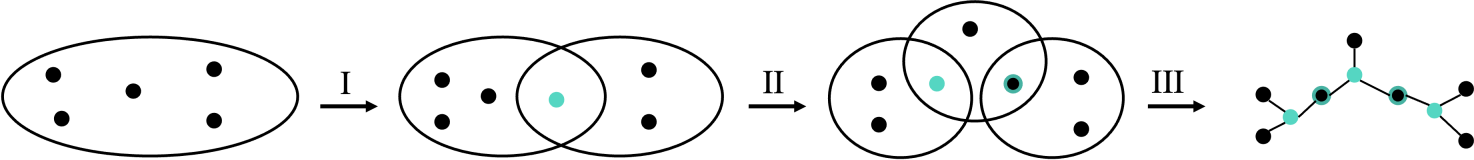
Figure 2: Example of reducing locality. Given a $\kappa=5$-local interaction on the Hamiltonian hypergraph. Applying the subdivision gadget from Lemma 22 reduces the locality to $\lceil 5/2\rceil=3$ (labelled I). Applying the subdivision gadget a further $O(\log\kappa)$ times yields a 3-local hypergraph (after II). Then the 3-to-2 gadget finally gives a 2-local Hamiltonian interaction graph (step III).

Interaction strength

By the triangle inequality $\norm{H_{\textup{target}}}=O(n\delta\mu_{0})$. The first round of perturbation theory has $\norm{H_{2}}<\norm{H_{1}}=O(\norm{H_{\textup{target}}})=O(n\delta\mu_{0})$ since $H_{1}$ includes $H_{\textup{else}}$. Hence $\Lambda_{1}=O(\norm{H_{\textup{target}}})=O(n\delta\mu_{0})$. For the first round of simulation, we can pick $\mu_{1}\propto\Lambda_{1}^{6}(\frac{1}{\epsilon^{2}}+\frac{1}{\eta^{2}})$ by Lemma 8.

For the second round, the new target Hamiltonian has $O(n\delta)+O(n\delta)$ terms of strength $O(\mu_{1})$, as each application of subdivision gadget adds $O(1)$ terms. Again $\norm{H_{1}}>\norm{H_{2}}$ giving $\Lambda_{2}\propto n\delta\mu_{1}$ and $\mu_{2}\propto\Lambda_{2}^{6}(\frac{1}{\epsilon^{2}}+\frac{1}{\eta^{2}})$.

Since this gadget will be applied $O(\kappa)$ times (some are applied in parallel so only $O(\log\kappa)$ rounds of perturbation in total), we can upper bound the number of terms by $O(n\delta\kappa)$. After $r$ rounds of simulation the interaction strength is

$$\mu_{r} \propto(n\delta\kappa)^{6r+1}\mu_{0}^{6r}\left(\frac{1}{\epsilon^{2}}+\frac{1}{\eta^{2}}\right)^{6(r-1)+1}$$ (69)

$$\in O\left((n\delta\kappa)^{6r+1}\left[\mu_{0}\left(\frac{1}{\epsilon^{2}}+\frac{1}{\eta^{2}}\right)\right]^{6r}\right)$$ (70)

$$\in O\left(\left[\operatorname{\mathrm{poly}}(n,\delta,\kappa)\mu_{0}\left(\frac{1}{\epsilon^{2}}+\frac{1}{\eta^{2}}\right)\right]^{6r}\right).$$ (71)

After the $\log(\kappa)$ rounds required to obtain a 2-local Hamiltonian, we obtain an interaction strength of

$$\mu\in O\left(\left[\operatorname{\mathrm{poly}}(n,\delta,\kappa)\mu_{0}\left(\frac{1}{\epsilon^{2}}+\frac{1}{\eta^{2}}\right)\right]^{6\log(\kappa)}\right).$$ (72)

Step 2 - Reduce degree

The ancillas introduced in step 1 have a maximum degree of $6$. After step 1 the degree of the original qubits is at most $3\delta$. We will use the triangle gadget (see Appendix A) to simulate $H^{\prime}$ by a 2-local Hamiltonian with degree $4$ denoted $H^{\prime\prime}$.

Lay out the $O(n\delta\kappa)$ qubits of $H^{\prime}$ in a line where each vertex in the graph has $O(\delta)$ incoming edges. Subdivide each edge just once so that the vertices with degree $>2$ are isolated on the line and interact only with an ancilla with degree 2 (this requires one round of simulation and $O(n\delta\kappa)$ ancillas). See Fig. 3 step I for reference.

Consider a given degree-$\delta$ vertex and the $O(\delta)$ ancillas it is directly connected to. $O(\log\delta)$ applications of the triangle gadget in parallel introduces $\log\delta$ ancillas and reduces the high degree vertex to $\delta/2$. Recursively iterating this procedure $O(\log\delta)$ times requires $O(\delta)$ ancillas and produces a tree of depth $O(\log\delta)$ which can be placed on a square lattice, resulting in an interaction graph with maximum degree $4$. See Fig. 3 step II for reference.

Individually executing this procedure for all high degree qubits in $H^{\prime}$ requires $O(n\kappa\delta^{2})$ ancillas and $O(\log\delta)$ rounds of perturbation.

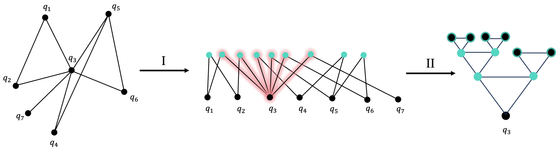
Figure 3: Example of reducing the degree in an interaction graph. Step I depicts subdividing all interactions once so every original qubit only shares an edge with a new ancilla (drawn in turquoise) that has degree 2. Each high degree qubit (in black) is then separately iterated with $O(\log\delta)$ applications of the triangle gadget (Lemma 23) yielding a graph with maimum degree 4. In II we have shown this procedure for one qubit $q_{3}$ but it will occur in parallel for all qubits on the line.

Interaction strength

After $\log(\delta)$ rounds, we will have introduced at most $O(n\delta\kappa)$ ancillas, and each has constant degree, thus the bound $\Lambda_{i+1}\propto n\delta\kappa\mu_{i}$ still holds, and we obtain

$$\mu\in O\left(\left[\operatorname{\mathrm{poly}}(n,\delta,\kappa)\mu_{0}\left(\frac{1}{\epsilon^{2}}+\frac{1}{\eta^{2}}\right)\right]^{6(\log(\kappa)+\log(\delta))}\right).$$ (73)

Step 3 - Making geometrically local

Now lay out the Hamiltonian from Step 2 on a 2D grid of size $O(n\kappa\delta)\times O(n\kappa\delta)$ Fig. 4. All interactions are 2 local and the maximum degree is 4. However the Hamiltonian graph is not geometrically local as interactions between qubits highlighted in blue may be $O(n\kappa\delta)$ long and there are many crossings.

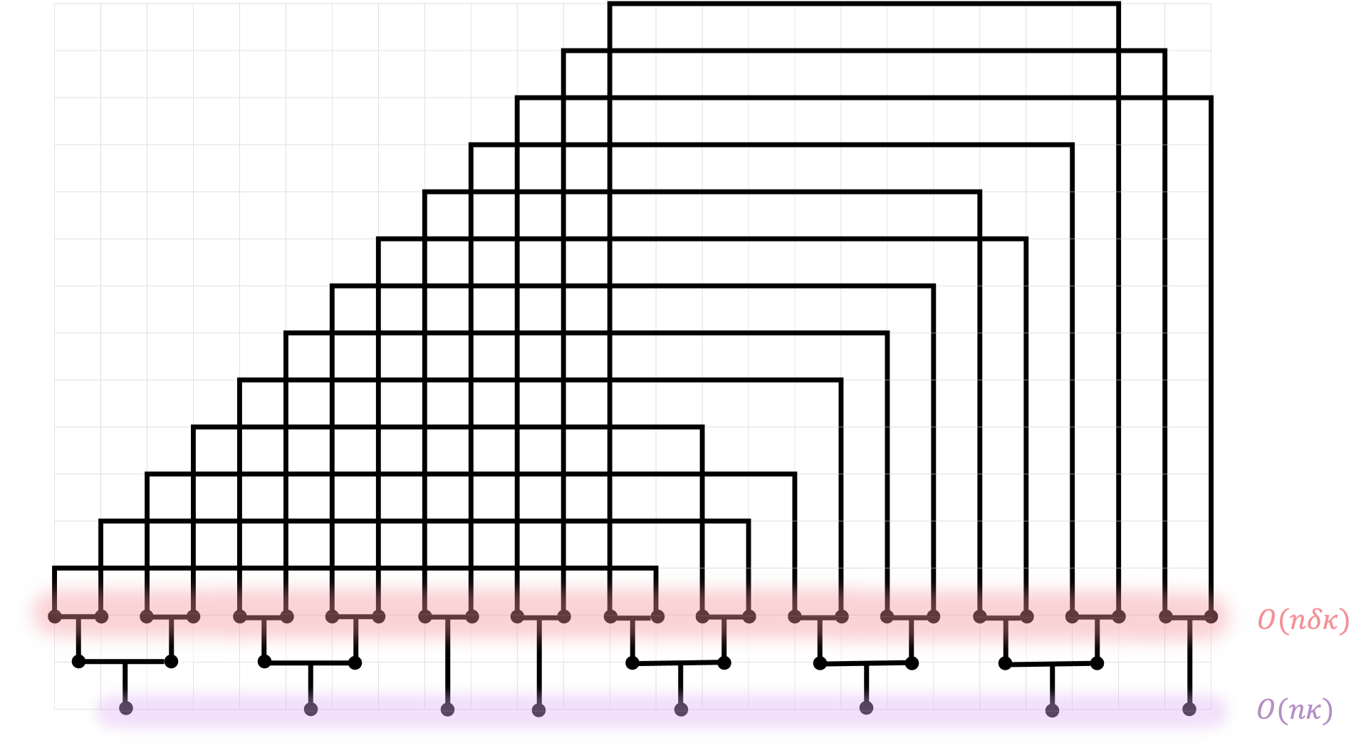
Figure 4: Lay out the Hamiltonian from step 2 on a 2d lattice. The qubits highlighted in pink are the qubits from step 1. In this example the maximum degree of the original graph was 4. The graph is not geometrically local due to the interactions between the blue qubits.

Step 3a - Remove long-range interactions

Generally the length of the edges in the graph after step 2 will be $O(n\kappa\delta)$, and these must now be fitted onto edges of the square lattice.

We can use one application of the newly introduced long-range gadget per long interaction which introduces the $O(n\kappa\delta)$ ancillas in a single round of perturbation.

Interaction strength

After applying a long-range gadget to each long-range edge on the interaction graph, we obtain at most $\propto(n\kappa\delta)^{2}$ ancillas – in the worst case filling up the $O(n\kappa\delta)\times O(n\kappa\delta)$ grid. Hence the norm of the Hamiltonian to be simulated at step $i$ is $\propto(n\delta\kappa)^{2}\mu_{i}$. However, we need to verify that $\Lambda_{i+1}$ upper bounds $\norm{H_{1}},\norm{H_{2}}$. $\norm{H_{2}}$ scales as $O(\sqrt{1/C})=O(\sqrt{n})$ from Lemma 15, and since $\norm{H_{1}}\leq\norm{H_{\textup{else}}}+\frac{D}{C}\propto(n\kappa\delta)^{2}\mu_{i}$, then $\max\{\norm{H_{1}},\norm{H_{2}}\}\leq(n\delta\kappa)^{2}\mu_{i}\propto\Lambda_{i+1}$. This does little to change the scaling of $\mu$: as we only need $O(1)$ rounds of simulation, obtaining

$$\mu\in O\left(\left[\operatorname{\mathrm{poly}}(n,\delta,\kappa)\mu_{0}\left(\frac{1}{\epsilon^{2}}+\frac{1}{\eta^{2}}\right)\right]^{6(\log(\kappa)+\log(\delta)+O(1))}\right).$$ (74)

Step 3b - Remove crossings

We have introduced a potential $O(n\kappa\delta)$ crossings per qubit at the leaves of the tree. Hence $O(n^{2}\kappa^{2}\delta^{2})$ crossings in the whole interaction graph.

Each crossing can be removed individually by $O(n^{2}\kappa^{2}\delta^{2})$ parallel applications of the crossing gadget (Appendix A). This introduces $O((n\kappa\delta)^{2})$ new ancillas but only requires $O(1)$ round of perturbation.

Interaction strength

The argument follows identically to the previous step. We obtain

$$\mu\in O\left(\left[\operatorname{\mathrm{poly}}(n,\delta,\kappa)\mu_{0}\left(\frac{1}{\epsilon^{2}}+\frac{1}{\eta^{2}}\right)\right]^{6(\log(\kappa)+\log(\delta)+O(1))}\right).$$ (75)

At the end of this procedure we obtain $H_{\textup{sim}}$ acting on a 2D grid of $O(n\kappa\delta)\times O(n\kappa\delta)$ qubits that simulates $H_{\textup{target}}$ with simulation parameters $(\mu/2,\eta,\epsilon)$. At each stage of simulation we use a perturbation gadget (Lemmas 22, 23, 16 and 24) which fit the definition of an approximate simulation (Definition 6) with $p=1$, $q=0$ and the isometry $T|\psi\rangle\mapsto|\psi\rangle\otimes|\text{anc}\rangle$. We either apply these gadgets in parallel (see Section 2 and references within) or in series requiring multiple rounds of perturbation.

The isometry for the simulation describing all gadgets applied in parallel is again of the form $T:|\psi\rangle\mapsto|\psi\rangle\otimes|\text{anc}\rangle$ if this is the case for each individual gadget. This can be seen since the projector into the joint ancillary groundspace is given by $P_{-}=\prod_{i}P_{-}^{(i)}$. All $P_{-}^{(i)}$ are rank one projectors acting on the subset $S_{i}$ and act trivially on the rest of the ancillas where $S_{i}$ are disjoint subsets of ancillary qubits. Thus, $P_{-}$ is a rank one projector acting on all ancillas inserted at that level: $S_{1}\cup S_{2}\cup...\cup S_{k}$. Similarly the isometry of the simulation describing the concatenation of two simulations is of the form $T:|\psi\rangle\mapsto|\psi\rangle\otimes|\text{anc}\rangle$ if this is the case for the component simulations. When we concatenate approximate simulations i.e. let A be a simulation of B and B be a simulation of C as in Lemma 9 we use the composed encoding map $\mathcal{E}=\mathcal{E}_{A}\circ\mathcal{E}_{B}$. Where $\mathcal{E}_{B}:\mathcal{H}\mapsto\mathcal{H}\otimes\mathcal{B}$ and $\mathcal{E}_{A}:(\mathcal{H}\otimes\mathcal{B})\mapsto(\mathcal{H}\otimes\mathcal{B})\otimes\mathcal{A}$ with $\mathcal{E}_{B}(M)=T_{B}MT_{B}^{\dagger}=M\otimes P_{B}$ and $\mathcal{E}_{A}(M)=T_{A}MT_{A}^{\dagger}=M\otimes P_{A}$. Then $\mathcal{E}_{A}\circ\mathcal{E}_{B}(M)=M\otimes P_{A}\otimes P_{B}$ and again due to multiplicative rank under Kronecker product $P_{A}\otimes P_{B}$ is rank 1 and we can describe $\mathcal{E}(M)=TMT^{\dagger}$ where $T:|\psi\rangle\mapsto|\psi\rangle\otimes|\text{anc}\rangle_{AB}$ for some pure state $|\text{anc}\rangle$. ∎

4.1 Arbitrary sparse Hamiltonians

Previously ‘efficient’ simulations by 2D lattice Hamiltonians constructed from gadgets were accessible to spatially sparse Hamiltonians (see Lemma 47 of [12]) but introducing long interactions caused an exponential increase in the required interaction strengths. [9] constructed efficient simulations for all local Hamiltonians using a history state method. Our new gadget is an exponential advantage over existing gadgets for this reduction and a polynomial improvement on the ancillas required compared to the previous efficient simulation. This facilitates a constructive simulation of arbitrary sparse Hamiltonians on a 2D lattice using only polynomial interaction strengths and quadratically many ancillas. Furthermore the number of ancillas in this work is independent of the simulation error. This is interesting from an analogue simulation perspective since general sparse Hamiltonians are now – at lease theoretically – accessible to restricted simulator Hamiltonians with simple connectivity.

We summarise this as a simple corollary of Theorem 17:

Corollary 18 (Simulating sparse Hamiltonians).

Given a Hamiltonian, $H=\sum_{i}h_{i}$, acting on $n$ qubits where $h_{i}$ is a Pauli rank one operator. Let be $H$ be sparse: $O(1)$-local and the maximum degree is $O(1)$.

$\exists$ a nearest neighbour Hamiltonian acting on a 2D lattice of $N=O(n^{2})$ qubits, $\tilde{H}=\sum_{j}\tilde{h}_{j}$, that is a $(\Delta,\eta,\epsilon)$-simulation of $H$ with,

$$\mu \in O\left(\operatorname{\mathrm{poly}}\left(n,\mu_{0}\left(\frac{1}{\epsilon^{2}}+\frac{1}{\eta^{2}}\right)\right)\right)$$

$$\Delta =\mu/2$$

where $\mu=\max_{j}\norm{\tilde{h}_{j}}$, and $\mu_{0}=\max_{i}\norm{h_{i}}$. Further the encoding isometry has the form $T:|\psi\rangle\longrightarrow|\psi\rangle\otimes|\textup{anc}\rangle$ for some state of the ancillary qubits $|\textup{anc}\rangle$.

Proof.

The proof is immediate by employing Theorem 17 setting $\delta,\kappa\in O(1)$. ∎

5 LDPC codes in 2D

A code can be associated with a Hamiltonian. Given a generating set of stabilizers for a CSS code,

$$A_{r}\equiv\prod_{n\in N_{r}}X_{n} \qquad 1\leq r\leq R$$ (76)

$$B_{s}\equiv\prod_{n\in N_{s}}Z_{n} \qquad 1\leq s\leq S,$$ (77)

where $[A_{r},B_{s}]=0$ for all $r\in[1,R]$ and $s\in[1,S]$. The code Hamiltonian reads,

$$H=-a\sum_{r=1}^{R}A_{r}-b\sum_{s=1}^{S}B_{s},$$ (78)

for $a,b>0$.

We begin with the Hamiltonian $H_{\textup{LDPC}}$, corresponding to a good LDPC code acting on $n$ qubits. It has been shown by [3, 4] that ‘good’ codes exist with $O(n)$ stabilizers of constant weight. Consequently we obtain a $\kappa$-local Hamiltonian with $\kappa=O(1)$ with respect to $n$. Furthermore each qubit is acted on non-trivially by a constant number of the stabilizer terms and so the maximum degree of the interaction graph is $\delta=O(1)$ with respect to $n$. Crucially these codes do not have so called ‘spatially sparse’ interaction hypergraphs, since when planarised the edges are of length $O(n)$ with many crossings. Instead they have the key property of being expander. Hence using previous gadget techniques to planarise these Hamiltonians would require interaction strengths and therefore energy scaling exponentially in $n$.

Employing Corollary 18 to sparse Hamiltonians describing ‘good’ codes immediately gives us a 2D geometrically local Hamiltonian with approximately the same energy landscape using only polynomial interaction strengths. Crucially we also need to examine the eigenstates of the simulation and show that they are closely related to the eigenstates of the code.

We will use the Gentle Measurement Lemma to quantify how a measurement does not drastically disturb a state if the probability of a given outcome is high:

Lemma 19 (Gentle Measurement Lemma: [20]).

Consider a density operator $\rho$ and a measurement operator $M$ where $0\geq M\geq\mathds{1}$ (could be an element of a POVM). Suppose that $M$ has a large probability of detecting state $\rho$

$$\tr[M\rho]\geq 1-\epsilon,$$

where $0<\epsilon\leq 1$. Then the post measurement state $\rho^{\prime}:=\frac{\sqrt{M}\rho\sqrt{M}}{\tr[M\rho]}$ is close to the original state,

$$\norm{\rho-\rho^{\prime}}_{1}\leq 2\sqrt{\epsilon}.$$

In the following result we show two complementary conditions satisfied by simulations where the isometry is particularly simple (of the form $T:|\psi\rangle\mapsto|\psi\rangle\otimes|\textup{anc}\rangle$) – as is the case for all the gadgets used in Theorem 17. The first is that for any low energy state in the simulation subspace, their energy as measured by the simulation Hamiltonian is close to what would be measured by the target Hamiltonian. In particular, we would like to ensure that the ground states of $H_{\textup{sim}}$ are almost ground states of $H_{\textup{target}}$, hence "soundness". Conversely, we would also like to ensure that all ground states of $H_{\textup{target}}$ are indeed also ground states of $H_{\textup{sim}}$, hence "completeness".

Lemma 20.

Let $H_{s}$ be a ($\Delta,\epsilon,\eta$)- simulation of the target Hamiltonian $H_{t}$. The local Encoding $\mathcal{E}:\mathcal{H}\mapsto\mathcal{H}\otimes\mathcal{A}$ is described by $\mathcal{E}(M)=TMT^{\dagger}=M\otimes P_{A}$ where $M\in\mathcal{H}$ and $P_{A}\in\mathcal{A}$ and $P_{A}$ is a rank one projector. The general encoding mapping into the low-energy subspace is given by $\tilde{\mathcal{E}}(M)=\tilde{T}M\tilde{T}^{\dagger}$ with $\norm{T-\tilde{T}}\leq\eta$(see Definition 6).

Then, for all sufficiently small $\eta$, we have

1. Let $\rho\in\mathcal{S}(\mathcal{H}\otimes\mathcal{A})$ be low energy energy state $\tr(\rho H_{s})\leq\epsilon^{\prime}$ (with $\epsilon^{\prime}\ll\Delta$), then

   $$\tr(\tr_{\mathcal{A}}(\rho)H_{t})\leq 5\epsilon^{\prime}+\epsilon+O_{\downarrow}\left(\sqrt{\eta}\right)\norm{H_{t}}.$$

   A condition we call ‘soundness’.

2. For any state $\sigma\in\mathcal{S}(\mathcal{\mathcal{H}})$, there exists a state $\tilde{\sigma}\in\mathcal{S}(\mathcal{H}\otimes\mathcal{A})$, such that

   $$\norm{\tr_{\mathcal{A}}(\tilde{\sigma})-\sigma}_{1}\in O_{\downarrow}(\eta),$$

   and

   $$\absolutevalue{\tr(\tilde{\sigma}H_{s})-\tr(\sigma H_{t})}\leq\epsilon.$$

   A condition we call ‘completeness’.

Where $g(x)\in O_{\downarrow}(f(x))$ if there exists $c,$ $\delta$ such that for all $0<\absolutevalue{x}<\delta$ we have $\absolutevalue{g(x)}\leq c\cdot f(x)$. $\mathcal{S}(\mathcal{H})$ denotes the states in the Hilbert space $\mathcal{H}$.

Proof.

For the sake of clarity, we will use the notation $g(x)\in O_{\downarrow}(f(x))$ since we are interested in the small $\eta$, $\epsilon$ regime.

We prove the two statements in turn,

Proof of soundness

Denote by $\mathcal{D}$ the subset of states in $\mathcal{S}(\mathcal{H}\otimes\mathcal{A})$ that are in $\mathrm{supp}(P_{\leq\Delta})$. Then $\rho=(1-p)\rho_{1}+p\rho_{2}$ where $p\in[0,1]$ and $\rho_{1}\in\mathcal{D}$, $\rho_{2}\in\mathcal{S}(\mathcal{H}\otimes\mathcal{A})\setminus\mathcal{D}$. Due to the definition of simulation the energy of $\rho_{2}$ is lower bounded by $\tr(\rho_{2}H_{s})\geq\Delta$.

Since $\rho$ is a low energy state the probability of being in $\mathcal{S}(\mathcal{H}\otimes\mathcal{A})\setminus\mathcal{D}$ is then necessarily small, $p\leq\frac{\epsilon^{\prime}}{\Delta}$. Therefore $\exists$ a state $\phi\in\mathcal{D}$ that is close to $\rho$ in trace distance:

$$\norm{\rho-\phi}_{1}\leq\frac{2\epsilon^{\prime}}{\Delta}.$$ (79)

Given such a state $\phi$:

$$\tr(TT^{\dagger}\phi TT^{\dagger})=\tr(\tilde{T}\tilde{T}^{\dagger}\phi\tilde{T}^{\dagger}\tilde{T})+\tr(TT^{\dagger}\phi T^{\dagger}T-\tilde{T}\tilde{T}^{\dagger}\phi\tilde{T}^{\dagger}\tilde{T}).$$ (80)

We have $\tilde{T}\tilde{T}^{\dagger}\phi\tilde{T}\tilde{T}^{\dagger}=\phi$, since $\tilde{T}\tilde{T}^{\dagger}=\tilde{\mathcal{E}}(\mathds{1})=P_{\leq\Delta}$, therefore $\tr(\tilde{T}\tilde{T}^{\dagger}\phi\tilde{T}^{\dagger}\tilde{T})=1$. Since $\norm{\tilde{T}-T}\leq\eta$, using the triangle inequality we can see that that $\norm{\tilde{T}\tilde{T}^{\dagger}-{T}{T}^{\dagger}}\leq 2\eta+\eta^{2}$. This gives

$$\tr({T}{T}^{\dagger}\phi{T}{T}^{\dagger})\geq 1-r,$$ (81)

where $r=2\eta+\eta^{2}$. Finally by the Gentle Measurement Lemma 19,

$$\norm{\phi-\frac{{T}{T}^{\dagger}\phi{T}{T}^{\dagger}}{\tr({T}{T}^{\dagger}\phi{T}{T}^{\dagger})}}_{1}\leq 2\sqrt{r}.$$ (82)

Note that $\frac{{T}{T}^{\dagger}\phi{T}{T}^{\dagger}}{\tr({T}{T}^{\dagger}\phi{T}{T}^{\dagger})}=\tau\otimes P_{A}$. Let $\phi=\tau\otimes P_{A}+\delta$, and $\tr_{\mathcal{A}}(\phi)=\tau+\delta^{\prime}$, since the trace distance decreases under CPTP maps, we get $\norm{\delta^{\prime}}_{1}\leq\norm{\delta}_{1}\leq 2\sqrt{r}$.

Now, write $H_{s}|_{\leq\Delta}={T}H_{t}{T}^{\dagger}+H_{A}$, and claim that $\norm{H_{A}}\leq\epsilon+2\eta\norm{H_{t}}$ since

$$\norm{H_{s}|_{\leq\Delta}-{T}H_{t}{T}^{\dagger}} =\norm{H_{s}|_{\leq\Delta}-\mathcal{E}(H_{t})+\tilde{\mathcal{E}}(H_{t})-\tilde{\mathcal{E}}(H_{t})}$$ (83)

$$\leq\norm{H_{s}|_{\leq\Delta}-\tilde{\mathcal{E}}(H_{t})}+\norm{-\mathcal{E}(H_{t})+\tilde{\mathcal{E}}(H_{t})}$$ (84)

$$\leq\epsilon+2\eta\norm{H_{t}},$$ (85)

where the final line uses that $\norm{TH_{t}T^{\dagger}-\tilde{T}H_{t}\tilde{T}^{\dagger}}\leq(\norm{T}+\norm{\tilde{T}})\norm{T-\tilde{T}}\norm{H_{t}}$ (Lemma 18 from [12]) and $\norm{H_{s}|_{\leq\Delta}-\tilde{\mathcal{E}}(H_{t})}\leq\epsilon$ by definition.

We are now in a position to prove the first statement,

$$\absolutevalue{\tr(\rho H_{s})-\tr(\tr_{\mathcal{A}}(\rho)H_{t})} =\absolutevalue{\tr((\rho-\phi)H_{s})+\tr(\phi(H_{s}))-\tr(\tr_{\mathcal{A}}(\phi)H_{t})+\tr((\tr_{\mathcal{A}}(\phi)-\tr_{\mathcal{A}}(\rho))H_{t})}$$ (86)

$$\leq 2\epsilon^{\prime}+\frac{2\epsilon^{\prime}\norm{H_{t}}}{\Delta}+\absolutevalue{\tr(\phi(H_{s}))-\tr(\tr_{\mathcal{A}}(\phi)H_{t}))}.$$ (87)

We can upper bound,

$$\absolutevalue{\tr(\phi(H_{s}))-\tr(\tr_{\mathcal{A}}(\phi)H_{t}))} =\absolutevalue{\tr(\phi(TH_{t}T^{\dagger}+H_{A}))-\tr((\tau+\delta^{\prime})H_{t})}$$ (88)

$$=\absolutevalue{\tr((\tau\otimes P_{A}+\delta)(H_{t}\otimes P_{A}))+\tr(\phi H_{A}))-\tr(\tau H_{t})-\tr(\delta^{\prime}H_{t})}$$ (89)

$$=\absolutevalue{\tr(\tau H_{t})+\tr(\delta(H_{t}\otimes P_{A}))+\tr(\phi H_{A}))-\tr(\tau H_{t})-\tr(\delta^{\prime}H_{t})}$$ (90)

$$\leq\norm{\delta}_{1}\norm{H_{t}\otimes P_{A}}+\norm{\phi}_{1}\norm{H_{A}}+\norm{\delta^{\prime}}_{1}\norm{H_{t}}$$ (91)

$$\leq 2\sqrt{r}\norm{H_{t}}+\epsilon+2\eta\norm{H_{t}}+2\sqrt{r}\norm{H_{t}}$$ (92)

$$\leq\epsilon+(4\sqrt{r}+2\eta)\norm{H_{t}},$$ (93)

where eq. 90 uses that $\tr(P_{A}^{2})=1$ since it is a rank one projector.

Combining eq. 87 and eq. 93 gives the result.

Proof of completeness

For any state $\sigma\in\mathcal{S}(\mathcal{H})$

$$\tr(\tilde{T}\sigma\tilde{T}^{\dagger}H_{s}) =\tr(\tilde{T}\sigma\tilde{T}^{\dagger}H_{s}|_{\leq\Delta})$$ (94)

$$=\tr(\tilde{T}\sigma\tilde{T}^{\dagger}\tilde{T}H_{t}\tilde{T}^{\dagger})+\tr(\tilde{T}\sigma\tilde{T}^{\dagger}H_{B})$$ (95)

$$=\tr(\sigma H_{t})+\tr(\tilde{T}\sigma\tilde{T}^{\dagger}H_{B})$$ (96)

where $H_{s}|_{\leq\Delta}=\tilde{T}H_{t}\tilde{T}^{\dagger}+H_{B}$, where $\norm{H_{B}}\leq\epsilon$ by the definition of a $(\Delta,\epsilon,\eta)$-simulation We conclude that $\absolutevalue{\tr(\tilde{T}\sigma\tilde{T}^{\dagger}H_{s})-\tr(\sigma H_{t})}\leq\epsilon$ .

Write $\tilde{\sigma}=\tilde{T}\sigma\tilde{T}^{\dagger}$, then we also have

$$\norm{\tr_{\mathcal{A}}(\tilde{\sigma})-\sigma}_{1} \leq\norm{\tilde{\sigma}-\sigma\otimes P_{A}}_{1}$$ (97)

$$=\norm{\tilde{T}\sigma\tilde{T}^{\dagger}-T\sigma T^{\dagger}}_{1}$$ (98)

$$\in O_{\downarrow}(\eta).$$ (99)

∎

We can now summarise our main result concerning simulating LDPC codes in the following theorem.

Theorem 21 (Simulating LDPC codes).

Given a Pauli Hamiltonian $H=\sum_{i}h_{i}$ corresponding to an arbitrary LDPC code $\mathcal{C}$ acting on $n$ qubits, $\mathcal{H}=(\mathbb{C}^{2})^{\otimes n}$. There $\exists$ a 2D nearest-neighbour Hamiltonian, $\tilde{H}=\sum_{j}\tilde{h}_{j}$, acting on a lattice of $N\in O(n^{2})$ qubits, $\mathcal{H}\otimes\mathcal{A}=(\mathbb{C}^{2})^{\otimes N}$. $\tilde{H}$ is a $(\Delta,\eta,\epsilon)$-simulation of $H$ such that,

1. The interaction strength of $\tilde{H}$, denoted $\tilde{\mu}$, scales polynomially with $n$:

   $$\mu\in O\left(\operatorname{\mathrm{poly}}\left(n,\mu_{0}\left(\frac{1}{\epsilon^{2}}+\frac{1}{\eta^{2}}\right)\right)\right)$$

   where $\mu_{0}$ is the interaction strength of $H$.

2. The low-energy eigenspectrum of $\tilde{H}$ for eigenvalues $<\Delta$, for $\Delta=\mu/2$ is a controllable approximation of $H$:

   $$\absolutevalue{\lambda_{i}(H)-\lambda_{i}(\tilde{H})}\leq\epsilon,$$

   where we denote by $\lambda_{i}(H)$ the $i^{\text{th}}$ smallest eigenvalue of $H$.

3. The eigenvectors corresponding to the low energy subspace of $\tilde{H}$ (again $<\Delta$) are close to the corresponding eigenvectors of $H$. For sufficiently small

   1. Soundness: Let $\rho\in\mathcal{S}(\mathcal{H}\otimes\mathcal{A})$ be low energy energy state $\tr(\rho H_{s})\leq\epsilon^{\prime}$, then

      $$\tr(\tr_{\mathcal{A}}(\rho)H_{t})\leq 5\epsilon^{\prime}+\epsilon+O_{\downarrow}\left(\sqrt{\eta}\right)\norm{H_{t}}.$$

   2. Completeness: For any state $\sigma\in\mathcal{S}(\mathcal{\mathcal{H}})$, there exists a state $\tilde{\sigma}\in\mathcal{S}(\mathcal{H}\otimes\mathcal{A})$, such that

      $$\norm{\tr_{\mathcal{A}}(\tilde{\sigma})-\sigma}_{1}\in O_{\downarrow}(\eta),$$

      and

      $$\absolutevalue{\tr(\tilde{\sigma}H_{s})-\tr(\sigma H_{t})}\leq\epsilon.$$

   Where we denote by $\mathcal{S}(\mathcal{H})$ the set of states in the Hilbert space $\mathcal{H}$ and $g(x)\in O_{\downarrow}(f(x))$ if there exists $c,$ $\delta$ such that for all $0<\absolutevalue{x}<\delta$ we have $\absolutevalue{g(x)}\leq c\cdot f(x)$.

Proof.

In order to be LDPC the interaction graph of $H$ has locality $k\in O(1)$, maximum degree $\delta\in O(1)$ and is therefore sparse. We can thus use Corollary 18 to construct a 2D nearest neighbour $(\Delta,\eta,\epsilon)$-simulating Hamiltonian with interaction strengths as quoted in point (1).

For all the gadgets used $p=1$ and $q=0$, hence as a direct result of point (i) from Lemma 7 we find the low energy eigenspectrum is approximately preserved – point (2).

To prove (3) we use Lemma 20 and the form of the isometry given for the encoding in Corollary 18 is $T:|\psi\rangle\mapsto|\psi\rangle\otimes|\text{anc}\rangle$ and hence $\mathcal{E}(H)=THT^{\dagger}=H\otimes P_{A}$ where $P_{A}$ is a rank one projector. Finally to demonstrate the eigenvector relation we employ Lemma 20 which immediately gives the result. ∎

Additionally we can consider applying Lemma 20 to [9]. In the history state construction the isometry mapping from the target Hilbert space to the enlarged simulator Hilbert space can be made close to the form $V|\psi\rangle\mapsto|\psi\rangle\otimes|\text{anc}\rangle$ by increasing the idling time. Therefore, the simulation obeys the constraints of Lemma 20. This would yield a result similar in spirit to Theorem 21 with the key difference that the simulator Hamiltonian acts on $O(\mathrm{poly}(n,\epsilon^{-1}))$ qubits. The key advantage of using our perturbative protocol is the number of ancillas involved: the polynomial scaling has bounded degree 2 and is independent of the simulation error. Having a single lattice and Hamiltonian structure for different error tolerances is practially desirable for this application. We leave considering whether the techniques of [9] could be optimised for codes to future work.

Appendix A Other perturbative gadgets

In this section we give as reference proofs of the perturbation gadgets used in Theorem 17 that were taken directly from the literature. They all first appeared in [5], however the phrasing and proof technique given here follows [21]. The mechanism of these simpler gadgets is a useful insight into how the long-range gadget is constructed.

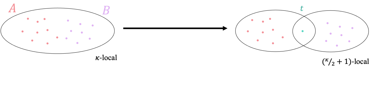
Figure 5: Subdivision gadget

Lemma 22 (Qubit subdivision gadget [21]).

The $\kappa$-local Hamiltonian,

$$H_{\textup{target}}=H_{\textup{else}}+P_{A}\otimes P_{B},$$ (100)

is $(\Delta/2,\eta,\epsilon)$-simulated by a $(\lfloor\kappa/2\rfloor+1)$-local Hamiltonian, $\tilde{H}=H+V$ where,

$$H=\Delta\Pi_{+}$$ (101)

$$V=H_{1}+\sqrt{\Delta}H_{2}$$ (102)

$$H_{1}=H_{\textup{else}}+\frac{1}{2}\left(P_{A}^{2}+P_{B}^{2}\right)$$ (103)

$$H_{2}=\frac{1}{\sqrt{2}}\left(P_{A}\otimes X_{t}-P_{B}\otimes X_{t}\right).$$ (104)

Hilbert space decomposition is given by,

$$\Pi_{-}=|0\rangle\bra{0}_{t}$$ (105)

$$\Pi_{+}=|1\rangle\bra{1}_{t}.$$ (106)

Proof.

Using the projectors given,

$$H_{1--}=\left(H_{\textup{else}}+2\mathds{1}\right)\otimes|0\rangle\bra{0}_{t}$$ (107)

$$H_{2-+}=H_{2+-}=\frac{1}{\sqrt{2}}\left(P_{A}-P_{B}\right)\otimes|0\rangle\bra{1}_{t}.$$ (108)

Therefore,

$$H_{2-+}H_{0}^{-1}H_{2+-} =\frac{1}{2}(P_{A}^{2}-P_{B}^{2})\otimes|0\rangle\bra{0}_{t}$$ (109)

$$=\left(\frac{1}{2}P_{A}^{2}-P_{A}\otimes P_{B}+\frac{1}{2}P_{B}^{2}\right)\otimes|0\rangle\bra{0}_{t}$$ (110)

Defining the isometry $T|\psi\rangle_{AB}=|\psi\rangle_{AB}|0\rangle_{t}$,

$$\norm{TH_{\textup{target}}T^{\dagger}-H_{1--}+H_{2-+}(H_{0++})^{-1}H_{2+-}}_{\infty}=0.$$ (111)

Therefore by Lemma 8 $\tilde{H}$ simulated $H_{\textup{target}}$ for any $\epsilon>0$ given an appropriate choice of $\Delta$. ∎

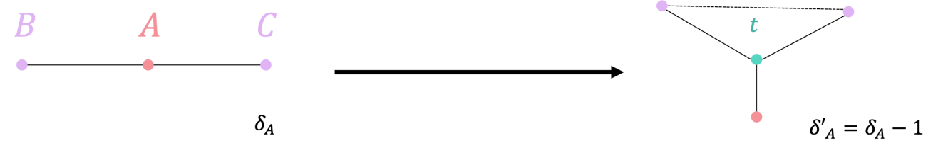
Figure 6: Triangle gadget

Lemma 23 (Triangle qubit gadget [21]).

The Hamiltonian where qubit $A$ has degree $\delta$ in the interaction graph,

$$H_{\textup{target}}=H_{\textup{else}}+\alpha_{ab}P_{A}\otimes P_{B}+\alpha_{ac}P_{A}\otimes,$$ (112)

is $(\Delta/2,\eta,\epsilon)$-simulated by a Hamiltonian, $\tilde{H}=H+V$, where qubit $A$ has degree $(\delta-1)$.

$$H=\Delta\Pi_{+}$$ (113)

$$V=H_{1}+\sqrt{\Delta}H_{2}$$ (114)

$$H_{1}=H_{\textup{else}}+\alpha_{ab}\alpha_{bc}P_{B}\otimes P_{C}^{\dagger}+\frac{1}{2}\left(1+\alpha_{ab}^{2}+\alpha_{bc}^{2}\right)\mathds{1}$$ (115)

$$\begin{multlined}H_{2}=\frac{1}{\sqrt{2}}\left(-P_{A}+\alpha_{ab}P_{B}+\alpha_{ac}P_{C}\right)\otimes X_{t}^{\dagger},\end{multlined}H_{2}=\frac{1}{\sqrt{2}}\left(-P_{A}+\alpha_{ab}P_{B}+\alpha_{ac}P_{C}\right)\otimes X_{t}^{\dagger},$$ (117)

where $X$ is the qubit Pauli X operator. Hilbert space decomposition is again given by,

$$\Pi_{-}=|0\rangle\bra{0}_{t}$$ (118)

$$\Pi_{+}=|1\rangle\bra{1}_{t}.$$ (119)

Proof.

Again using the projectors given,

$$H_{1--}=H_{1}\otimes|0\rangle\bra{0}_{t}$$ (120)

$$\begin{multlined}H_{2-+}=\frac{1}{\sqrt{2}}\left(-P_{A}+\alpha_{ab}P_{B}+\alpha_{ac}P_{C}\right)\otimes|0\rangle\bra{p-1}_{t}.\end{multlined}H_{2-+}=\frac{1}{\sqrt{2}}\left(-P_{A}+\alpha_{ab}P_{B}+\alpha_{ac}P_{C}\right)\otimes|0\rangle\bra{p-1}_{t}.$$ (122)

Therefore,

$$\begin{multlined}(H_{2})_{-+}(H_{0})^{-1}(H_{2})_{+-}=\frac{1}{2}(P_{A}^{2}+\alpha_{ab}^{2}P_{B}^{2}+\alpha_{bc}^{2}P_{C}^{2})-2\alpha_{ab}P_{A}\otimes P_{B}-2\alpha_{ac}P_{A}\otimes P_{C}\\ +2\alpha_{ab}\alpha_{bc}P_{B}\otimes P_{C}.\end{multlined}(H_{2})_{-+}(H_{0})^{-1}(H_{2})_{+-}=\frac{1}{2}(P_{A}^{2}+\alpha_{ab}^{2}P_{B}^{2}+\alpha_{bc}^{2}P_{C}^{2})-2\alpha_{ab}P_{A}\otimes P_{B}-2\alpha_{ac}P_{A}\otimes P_{C}\\ +2\alpha_{ab}\alpha_{bc}P_{B}\otimes P_{C}.$$ (123)

Defining the isometry $T|\psi\rangle_{AB}=|\psi\rangle_{AB}|0\rangle_{t}$,

$$\norm{TH_{\textup{target}}T^{\dagger}-H_{1--}+H_{2-+}(H_{0++})^{-1}H_{2+-}}_{\infty}=0.$$ (124)

Therefore by Lemma 8 $\tilde{H}$ simulated $H_{\textup{target}}$ for any $\epsilon>0$ given an appropriate choice of $\Delta$. ∎

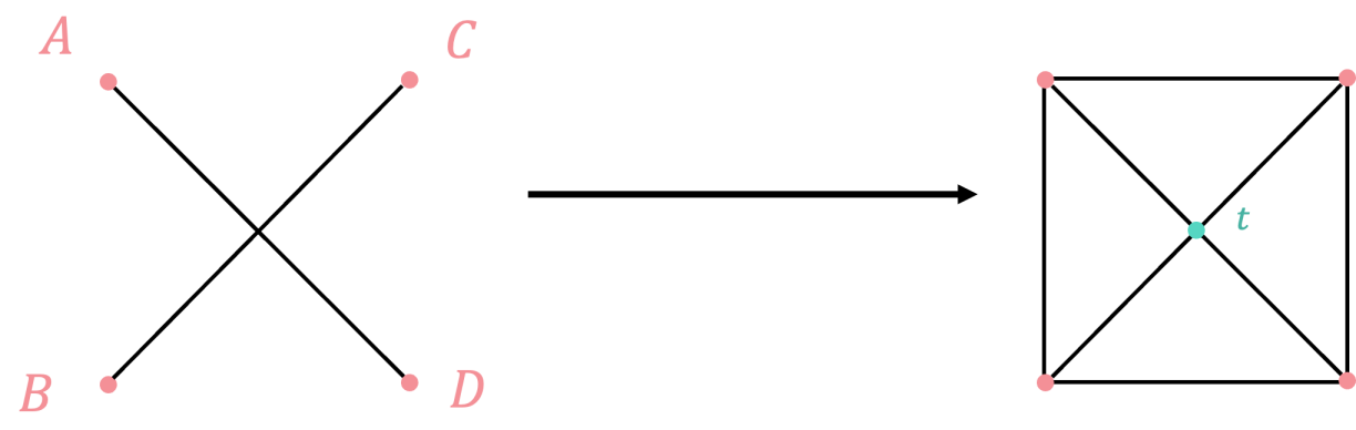
Figure 7: Crossing gadget

Lemma 24 (Qubit crossing gadget [5]).

The ‘crossed’ Hamiltonian,

$$H_{\textup{target}}=H_{\textup{else}}+\alpha_{ad}P_{A}\otimes P_{D}+\alpha_{bc}P_{B}\otimes P_{C},$$ (125)

is $(\Delta/2,\eta,\epsilon)$-simulated by a geometrically local Hamiltonian, $\tilde{H}=H+V$ where,

$$H=\Delta\Pi_{+}$$ (126)

$$V=H_{1}+\sqrt{\Delta}H_{2}$$ (127)

$$\begin{multlined}H_{1}=H_{\textup{else}}+\frac{1}{2}\left(\alpha_{ad}P_{A}^{2}+\alpha_{bc}P_{B}^{2}+P_{C}^{2}+P_{D}^{2}\right)-\alpha_{ad}\alpha_{bc}P_{A}\otimes P_{B}+\alpha_{ad}P_{A}\otimes P_{C}\\ +\alpha_{bc}P_{B}\otimes P_{D}-P_{C}\otimes P_{D}\end{multlined}H_{1}=H_{\textup{else}}+\frac{1}{2}\left(\alpha_{ad}P_{A}^{2}+\alpha_{bc}P_{B}^{2}+P_{C}^{2}+P_{D}^{2}\right)-\alpha_{ad}\alpha_{bc}P_{A}\otimes P_{B}+\alpha_{ad}P_{A}\otimes P_{C}\\ +\alpha_{bc}P_{B}\otimes P_{D}-P_{C}\otimes P_{D}$$ (130)

$$H_{2}=\frac{1}{\sqrt{2}}\left(-\alpha_{ad}P_{A}\otimes X_{t}-\alpha_{bc}P_{B}\otimes X_{t}+P_{C}\otimes X_{t}+P_{D}\otimes X_{t}\right).$$ (131)

Hilbert space decomposition is given by,

$$\Pi_{-}=|0\rangle\bra{0}_{t}$$ (132)

$$\Pi_{+}=|1\rangle\bra{1}_{t}.$$ (133)

Proof.

This is a second order simulation.

$$(H_{2})_{-+}=\frac{1}{\sqrt{2}}\left[-\alpha_{ad}P_{A}\otimes-\alpha_{bc}P_{B}+P_{C}+P_{D}\right]|0\rangle\bra{1}_{t}.$$ (134)

Therefore,

$$\begin{multlined}(H_{2})_{-+}(H_{0})^{-1}(H_{2})_{+-}=\frac{1}{2}\left[\alpha_{ad}^{2}P_{A}^{2}+\alpha_{bc}^{2}P_{B}^{2}+P_{C}^{2}+P_{D}^{2}+2\alpha_{ad}\alpha_{bc}P_{A}\otimes P_{B}-2\alpha_{ad}P_{A}\otimes P_{C}\right.\\ \left.-2\alpha_{ad}P_{A}\otimes P_{D}-2\alpha_{bc}P_{B}\otimes P_{C}-2\alpha_{bc}P_{B}\otimes P_{D}+2P_{c}\otimes P_{D}\right]|0\rangle\bra{0}_{t}.\end{multlined}(H_{2})_{-+}(H_{0})^{-1}(H_{2})_{+-}=\frac{1}{2}\left[\alpha_{ad}^{2}P_{A}^{2}+\alpha_{bc}^{2}P_{B}^{2}+P_{C}^{2}+P_{D}^{2}+2\alpha_{ad}\alpha_{bc}P_{A}\otimes P_{B}-2\alpha_{ad}P_{A}\otimes P_{C}\right.\\ \left.-2\alpha_{ad}P_{A}\otimes P_{D}-2\alpha_{bc}P_{B}\otimes P_{C}-2\alpha_{bc}P_{B}\otimes P_{D}+2P_{c}\otimes P_{D}\right]|0\rangle\bra{0}_{t}.$$ (135)

Defining the isometry $T:|\psi\rangle_{ABCD}\mapsto|\psi\rangle_{ABCD}\otimes|0\rangle_{t}$ then,

$$\norm{TH_{\textup{target}}T^{\dagger}-H_{1--}+H_{2-+}(H_{0++})^{-1}H_{2+-}}_{\infty}=0.$$ (136)

Therefore by Lemma 8 $\tilde{H}$ simulated $H_{\textup{target}}$ for any $\epsilon>0$ given an appropriate choice of $\Delta$. ∎

Lemma 25 (Third order simulation [13]).

Let $V=H_{1}+\Delta^{\frac{1}{3}}H_{1}^{\prime}+\Delta^{\frac{2}{3}}H_{2}$ be a perturbation action on the same space as $H_{0}$ such that $\max\{\norm{H_{1}},\norm{H_{1}^{\prime}},\norm{H_{2}}\}\leq\Lambda$; $H_{1}$ and $H_{1}^{\prime}$ are block diagonal with respect to the split $\mathcal{H}=\mathcal{H}_{-}\oplus\mathcal{H}_{+}$ and $(H_{2})_{--}=0$. Suppose there exists an isometry $T$ such that $\operatorname{Im}(T)=\mathcal{H}_{-}$ and:

$$\norm{TH_{\textup{target}}T^{\dagger}-(H_{1})_{--}+(H_{2})_{-+}H_{0}^{-1}(H_{2})_{++}H_{0}^{-1}(H_{2})_{+-}}_{\infty}\leq\frac{\epsilon}{2}$$ (137)

and also that:

$$(H_{1}^{\prime})_{--}=(H_{2})_{{}_{+}}H_{0}^{-1}(H_{2})_{+-}.$$ (138)

Then $\tilde{H}$ is a $\left(\frac{\Delta}{2},\eta,\epsilon\right)$-simulation of $H_{\textup{target}}$ provided that $\Delta\geq O\left(\frac{\Lambda^{12}}{\epsilon^{3}}+\frac{\Lambda^{3}}{\eta^{3}}\right)$.

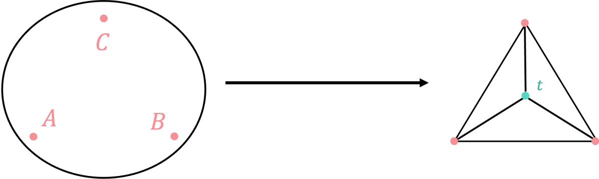
Figure 8: 3-to-2 qubit gadget.

Lemma 26 (Qubit 3-to-2 gadget [5]).

The $3$-local Hamiltonian,

$$H_{\textup{target}}=H_{\textup{else}}+P_{A}\otimes P_{B}\otimes P_{C},$$ (139)

is $(\Delta/2,\eta,\epsilon)$-simulated by a $2$-local Hamiltonian, $\tilde{H}=H+V$ where,

$$H=\Delta\Pi_{+}$$ (140)

$$V=H_{1}+\Delta^{1/3}H_{1}^{\prime}+\Delta^{2/3}H_{2}$$ (141)

$$H_{1}=H_{\textup{else}}+\frac{1}{2}\left(P_{A}^{2}+P_{B}^{2}\right)\otimes P_{C}$$ (142)

$$H_{1}^{\prime}=\frac{1}{2}\left(-P_{A}+P_{B}\right)^{2}$$ (143)

$$H_{2}=P_{C}\otimes|1\rangle\bra{1}_{t}+\frac{1}{\sqrt{2}}\left(-P_{A}\otimes X_{t}+P_{B}\otimes X_{t}\right).$$ (144)

Hilbert space decomposition is given by,

$$\Pi_{-}=|0\rangle\bra{0}_{t}$$ (145)

$$\Pi_{+}=|1\rangle\bra{1}_{t}.$$ (146)

Proof.

This is a third order simulation so to prove the above we need to demonstrate the construction satisfies the two conditions of Lemma 25.

$$(H_{2})_{-+}=\frac{1}{\sqrt{2}}\left[(-P_{A}+P_{B})\otimes|0\rangle\bra{1}_{t}\right],$$ (147)

Therefore,

$$(H_{2})_{-+}H_{)}^{-1}(H_{2})_{+-}=\frac{1}{2}\left[(-P_{A}+P_{B})^{2}\otimes|0\rangle\bra{0}_{t}\right]=(H_{1}^{\prime})_{--}.$$ (148)

Then,

$$(H_{2})_{++}=P_{C}\otimes|1\rangle\bra{1}_{t},$$ (149)

so that,

$$(H_{2})_{-+}H_{0}^{-1}(H_{2})_{++}H_{0}^{-1}(H_{2})_{+-} =\frac{1}{2}\left[(-P_{A}+P_{B})\otimes|0\rangle\bra{1}_{w}\right]\left[P_{C}\otimes|1\rangle\bra{1}_{w}\right]\left[(-P_{A}+P_{B})\otimes|1\rangle\bra{0}\right]$$ (150)

$$=\left[-P_{A}\otimes P_{B}\otimes P_{C}+\frac{1}{2}(P_{A}^{2}+P_{B}^{2})\otimes P_{C}\right]\otimes|0\rangle\bra{0}_{t}.$$ (151)

Defining the isometry $T|\psi\rangle_{ABC}=|\psi\rangle_{ABC}|0\rangle_{t}$, eq. 137 vanishes,

$$\norm{TH_{\textup{target}}T^{\dagger}-(H_{1})_{--}+(H_{2})_{-+}H_{0}^{-1}(H_{2})_{++}H_{0}^{-1}(H_{2})_{+-}}_{\infty}=0.$$ (152)

Therefore by Lemma 25 $\tilde{H}$ simulated $H_{\textup{target}}$ for any $\epsilon>0$ given an appropriate choice of $\Delta$. ∎

Appendix B Impossibility of a gapped Hamiltonian

This section considers the extent to which our result can be improved using similar methods. In particular, one could

1. Substitute $X_{i},X_{j}$ for different operators $\Gamma_{i},\Gamma_{j}$ that potentially act on multiple qubits

2. Pick a better ancilla state than $|W\rangle$, or a better parent Hamiltonian for $H_{W}$, or a combination of both.

Unfortunately, we will show that even given this flexibility, the interaction strength of the simulation Hamiltonian of the long range gadget has to scale like $\widetilde{\Omega}(n)$.

Henceforth consider $\Gamma_{i},\Gamma_{j}$ operators acting on a disc of radius $O(1)$. Instead of $|W\rangle$, we focus on $|\psi\rangle$, the unique ground state of an arbitrary Hamiltonian $H_{\psi}$ with spectral gap at least $1$. For simplicity, we take $H_{\textup{else}}=0$, and following the method of Section 3 we assume that the simulation Hamiltonian obeys :

$$H_{1}=\frac{D^{\prime}}{C^{\prime}}(P_{A}^{2}\otimes P_{B}^{2})$$ (153)

$$H_{2}=\frac{1}{\sqrt{C^{\prime}}}(P_{A}\otimes\Gamma_{i}-P_{B}\otimes\Gamma_{j}),$$ (154)

with

$$D^{\prime} =\bra{\psi}\Gamma_{i}(H_{\psi++})^{-1}\Gamma_{i}|\psi\rangle+\bra{\psi}\Gamma_{j}(H_{\psi++})^{-1}\Gamma_{j}|\psi\rangle$$ (155)

$$C^{\prime} =\bra{\psi}\Gamma_{i}(H_{\psi++})^{-1}\Gamma_{j}|\psi\rangle+\bra{\psi}\Gamma_{j}(H_{\psi++})^{-1}\Gamma_{i}|\psi\rangle.$$ (156)

It would technically be possible to pick different pre-factors for $H_{1},H_{2}$ but the end result would not be significantly affected. Similarly to Theorem 16, we define $\Pi_{-}=\outerproduct{\psi}{\psi}$, $\Pi_{+}=\mathds{1}-\Pi_{-}$, and $H_{\psi++}=\Pi_{+}H_{\psi}\Pi_{+}$,

$$\begin{multlined}H_{2-+}(H_{W++})^{-1}H_{2+-}=\frac{1}{C^{\prime}}\left[\mathbf{1}_{AB}\otimes\left(\Pi_{-}\Gamma_{i}\Pi_{+}(H_{\psi++})^{-1}\Pi_{+}\Gamma_{i}\Pi_{-}+\Pi_{-}\Gamma_{j}\Pi_{+}(H_{\psi++})^{-1}\Pi_{+}\Gamma_{j}\Pi_{-}\right)\right.\\ \left.-P_{A}\otimes P_{B}\otimes\left(\Pi_{-}\Gamma_{i}\Pi_{+}(H_{\psi++})^{-1}\Pi_{+}\Gamma_{j}\Pi_{-}+\Pi_{-}\Gamma_{j}\Pi_{+}(H_{\psi++})^{-1}\Pi_{+}\Gamma_{i}\Pi_{-}\right)\right].\end{multlined}H_{2-+}(H_{W++})^{-1}H_{2+-}=\frac{1}{C^{\prime}}\left[\mathbf{1}_{AB}\otimes\left(\Pi_{-}\Gamma_{i}\Pi_{+}(H_{\psi++})^{-1}\Pi_{+}\Gamma_{i}\Pi_{-}+\Pi_{-}\Gamma_{j}\Pi_{+}(H_{\psi++})^{-1}\Pi_{+}\Gamma_{j}\Pi_{-}\right)\right.\\ \left.-P_{A}\otimes P_{B}\otimes\left(\Pi_{-}\Gamma_{i}\Pi_{+}(H_{\psi++})^{-1}\Pi_{+}\Gamma_{j}\Pi_{-}+\Pi_{-}\Gamma_{j}\Pi_{+}(H_{\psi++})^{-1}\Pi_{+}\Gamma_{i}\Pi_{-}\right)\right].$$ (157)

Assuming that $C^{\prime}\neq 0$, we can verify that the gadget works via Lemma 8, as:

$$\norm{TH_{\textup{target}}T^{\dagger}-H_{1--}+H_{2-+}(H_{W++})^{-1}H_{2+-}}=0.$$ (158)

We can now detail our argument. The interaction strength of the simulation Hamiltonian is lower bounded by $\max(1/\sqrt{C^{\prime}},\mu_{\psi})$, where $\mu_{\psi}$ is the interaction strength of $H_{\psi}$. Since $\tilde{H}=\Delta H_{0}+H_{1}+\sqrt{\Delta}H_{2}$ and we have assumed $\Delta\geq 1$. Obtaining a large $C^{\prime}$ requires that $H_{\psi}$ has large interaction strength. The crux of the argument is that $\bra{\psi}\Gamma_{i}(H_{\psi++})^{-1}\Gamma_{j}|\psi\rangle$ is essentially a correlation function weighted by the inverse Hamiltonian, and systems with a large correlation functions need large interaction strengths.

Recall from the definition of $C^{\prime}$,

$$C^{\prime} =\bra{\psi}\Gamma_{i}(H_{\psi++})^{-1}\Gamma_{j}|\psi\rangle+\bra{\psi}\Gamma_{j}(H_{\psi++})^{-1}\Gamma_{i}|\psi\rangle$$ (159)

$$=2\textup{Re}(\bra{\psi}\Gamma_{i}(H_{\psi++})^{-1}\Gamma_{j}|\psi\rangle)$$ (160)

$$\leq 2|\bra{\psi}\Gamma_{i}(H_{\psi++})^{-1}\Gamma_{j}|\psi\rangle|$$ (161)

$$=2\sqrt{\bra{\psi}\Gamma_{i}(H_{\psi++})^{-1}\Gamma_{j}|\psi\rangle\bra{\psi}\Gamma_{j}(H_{\psi++})^{-1}\Gamma_{i}|\psi\rangle}.$$ (162)

Now we focus on the operator $(H_{\psi++})^{-1}\Gamma_{j}|\psi\rangle\bra{\psi}\Gamma_{j}(H_{\psi++})^{-1}$, since

$$\norm{H_{\psi++}}^{-1}\Pi_{+}\leq(H_{\psi++})^{-1}\leq\Pi_{+},$$ (163)

where for two operators $A,B$, we say $A\geq B$ if $A-B\geq 0$, i.e. if $A-B$ is positive semi-definite. Then

$$\norm{H_{\psi++}}^{-2}\Pi_{+}\Gamma_{j}|\psi\rangle\bra{\psi}\Gamma_{j}\Pi_{+}\leq(H_{\psi++})^{-1}\Gamma_{j}|\psi\rangle\bra{\psi}\Gamma_{j}(H_{\psi++})^{-1}\leq\Pi_{+}\Gamma_{j}|\psi\rangle\bra{\psi}\Gamma_{j}\Pi_{+}$$ (164)

We get

$$\bra{\psi}\Gamma_{i}(H_{\psi++})^{-1}\Gamma_{j}|\psi\rangle\bra{\psi}\Gamma_{j}(H_{\psi++})^{-1}\Gamma_{i}|\psi\rangle\leq\bra{\psi}\Gamma_{i}\Pi_{+}\Gamma_{j}|\psi\rangle\bra{\psi}\Gamma_{j}\Pi_{+}\Gamma_{i}|\psi\rangle.$$ (165)

Note that $\bra{\psi}\Gamma_{i}\Pi_{+}\Gamma_{j}|\psi\rangle=\bra{\psi}\Gamma_{i}\otimes\Gamma_{j}|\psi\rangle-\bra{\psi}\Gamma_{i}\outerproduct{\psi}{\psi}\Gamma_{j}|\psi\rangle$ is indeed the usual correlation function. From Theorem 4 of [10] and the fact that without loss of generality, we can take the distance between $\Gamma_{i}$ and $\Gamma_{j}$ to be $\Omega(n)$ – we obtain:

$$\absolutevalue{\bra{\psi}\Gamma_{i}\Pi_{+}\Gamma_{j}|\psi\rangle}\in O\left(\norm{\Gamma_{i}}\norm{\Gamma_{j}}e^{-\Omega(n/\mu_{\psi})}\right).$$ (166)

This yields the desired result:

$$C^{\prime}\in O\left(\norm{\Gamma_{i}}\norm{\Gamma_{j}}e^{-\Omega(n/\mu_{\psi})}\right).$$ (167)

Assuming that $\norm{\Gamma_{i}},\norm{\Gamma_{j}}$ scale at most polynomially, the interaction strength of the simulation Hamiltonian can be lower bounded by

$$\max\left(\mu_{\psi},\Omega(e^{\Omega(n/\mu_{\psi})}/\operatorname{\mathrm{poly}}(n))\right)\leq\max\norm{\tilde{h}_{i}}.$$ (168)

We can read off from the above equation that $\mu_{\psi}$ has to scale like $\in\widetilde{\Omega}(n)$ for $1/\sqrt{C^{\prime}}$ to scale polynomially.

Appendix C Tighter estimation of the gap

We remind the reader of the following expression for $\Pi_{\mathcal{A}\cup\mathcal{B}}-\Pi_{\mathcal{A}}\Pi_{\mathcal{B}}$:

$$\begin{multlined}\Pi_{\mathcal{A}\cup\mathcal{B}}-\Pi_{\mathcal{A}}\Pi_{\mathcal{B}}=\left(\frac{\sqrt{a\bar{b}}}{m}-\sqrt{\frac{\bar{b}}{a}}\right)|W\rangle_{\mathcal{A}}|0\rangle_{\bar{\mathcal{A}}}\bra{W}_{\bar{\mathcal{B}}}\bra{0}_{\mathcal{B}}+\left(\frac{\sqrt{ab}}{m}-\frac{l}{\sqrt{ab}}\right)|W\rangle_{\mathcal{A}}|0\rangle_{\bar{\mathcal{A}}}\bra{0}_{\bar{\mathcal{B}}}\bra{W}_{\mathcal{B}}\\ +\left(\frac{\sqrt{\bar{a}b}}{m}-\sqrt{\frac{\bar{a}}{b}}\right)|0\rangle_{\mathcal{A}}|W\rangle_{\bar{\mathcal{A}}}\bra{0}_{\bar{\mathcal{B}}}\bra{W}_{\mathcal{B}}+\frac{\sqrt{\bar{a}\bar{b}}}{m}|0\rangle_{\mathcal{A}}|W\rangle_{\bar{\mathcal{A}}}\bra{W}_{\bar{\mathcal{B}}}\bra{0}_{\mathcal{B}}-\frac{\sqrt{\bar{a}\bar{b}}}{\sqrt{ab}}|W\rangle_{\mathcal{A}}|W\rangle_{\bar{\mathcal{A}}}\bra{W}_{\bar{\mathcal{B}}}\bra{W}_{\mathcal{B}}.\end{multlined}\Pi_{\mathcal{A}\cup\mathcal{B}}-\Pi_{\mathcal{A}}\Pi_{\mathcal{B}}=\left(\frac{\sqrt{a\bar{b}}}{m}-\sqrt{\frac{\bar{b}}{a}}\right)|W\rangle_{\mathcal{A}}|0\rangle_{\bar{\mathcal{A}}}\bra{W}_{\bar{\mathcal{B}}}\bra{0}_{\mathcal{B}}+\left(\frac{\sqrt{ab}}{m}-\frac{l}{\sqrt{ab}}\right)|W\rangle_{\mathcal{A}}|0\rangle_{\bar{\mathcal{A}}}\bra{0}_{\bar{\mathcal{B}}}\bra{W}_{\mathcal{B}}\\ +\left(\frac{\sqrt{\bar{a}b}}{m}-\sqrt{\frac{\bar{a}}{b}}\right)|0\rangle_{\mathcal{A}}|W\rangle_{\bar{\mathcal{A}}}\bra{0}_{\bar{\mathcal{B}}}\bra{W}_{\mathcal{B}}+\frac{\sqrt{\bar{a}\bar{b}}}{m}|0\rangle_{\mathcal{A}}|W\rangle_{\bar{\mathcal{A}}}\bra{W}_{\bar{\mathcal{B}}}\bra{0}_{\mathcal{B}}-\frac{\sqrt{\bar{a}\bar{b}}}{\sqrt{ab}}|W\rangle_{\mathcal{A}}|W\rangle_{\bar{\mathcal{A}}}\bra{W}_{\bar{\mathcal{B}}}\bra{W}_{\mathcal{B}}.$$ (169)

This can be rewriten as

$$\Pi_{\mathcal{A}\cup\mathcal{B}}-\Pi_{\mathcal{A}}\Pi_{\mathcal{B}}=\lambda_{1}A_{1}+\lambda_{2}A_{2}+\lambda_{3}A_{3}+\lambda_{4}A_{4}+\lambda_{5}A_{5}$$ (170)

where $\lambda_{1}=\frac{\sqrt{a\bar{b}}}{m}-\sqrt{\frac{\bar{b}}{a}}$, $A_{1}=|W\rangle_{\mathcal{A}}|0\rangle_{\bar{\mathcal{A}}}\bra{W}_{\bar{\mathcal{B}}}\bra{0}_{\mathcal{B}}$, and similarly for the rest. Then,

$$\norm{\Pi_{\mathcal{A}\cup\mathcal{B}}-\Pi_{\mathcal{A}}\Pi_{\mathcal{B}}}_{\infty}= \norm{\sum_{i}\lambda_{i}A_{i}}=\max_{|x\rangle}\norm{\sum_{i}\lambda_{i}A_{i}|x\rangle}$$ (171)

$$= \max_{|x\rangle}\sqrt{\bra{x}\sum_{i}\lambda_{i}A_{i}^{\dagger}\sum_{j}\lambda_{j}A_{j}|x\rangle}.$$ (172)

Straightforward computation gives,

$$\sum_{i}\lambda_{i}A_{i}^{\dagger}\sum_{j}\lambda_{j}A_{j}=A^{\prime}\oplus A^{\prime\prime},$$ (173)

where

$$\begin{multlined}A^{\prime}=(\lambda_{2}^{2}+\lambda_{3}^{2})\outerproduct{0}{0}_{\bar{\mathcal{B}}}\otimes\outerproduct{W}{W}_{\mathcal{B}}+(\lambda_{1}\lambda_{2}+\lambda_{3}\lambda_{4})|0\rangle\bra{W}_{\bar{\mathcal{B}}}\otimes|W\rangle\bra{0}_{\mathcal{B}}\\ +(\lambda_{1}\lambda_{2}+\lambda_{3}\lambda_{4})|W\rangle\bra{0}_{\bar{\mathcal{B}}}\otimes|0\rangle\bra{W}_{\mathcal{B}}+(\lambda_{1}^{2}+\lambda_{4}^{2})\outerproduct{W}{W}_{\bar{\mathcal{B}}}\otimes\outerproduct{0}{0}_{\mathcal{B}},\end{multlined}A^{\prime}=(\lambda_{2}^{2}+\lambda_{3}^{2})\outerproduct{0}{0}_{\bar{\mathcal{B}}}\otimes\outerproduct{W}{W}_{\mathcal{B}}+(\lambda_{1}\lambda_{2}+\lambda_{3}\lambda_{4})|0\rangle\bra{W}_{\bar{\mathcal{B}}}\otimes|W\rangle\bra{0}_{\mathcal{B}}\\ +(\lambda_{1}\lambda_{2}+\lambda_{3}\lambda_{4})|W\rangle\bra{0}_{\bar{\mathcal{B}}}\otimes|0\rangle\bra{W}_{\mathcal{B}}+(\lambda_{1}^{2}+\lambda_{4}^{2})\outerproduct{W}{W}_{\bar{\mathcal{B}}}\otimes\outerproduct{0}{0}_{\mathcal{B}},$$ (174)

and

$$A^{\prime\prime}=\lambda_{5}^{2}\outerproduct{W}{W}_{\bar{\mathcal{B}}}\otimes\outerproduct{W}{W}_{\mathcal{B}}.$$ (175)

Since $A^{\prime}$ is hermitian, it can be diagonalized, $A^{\prime}=u_{1}\outerproduct{u_{1}}{u_{1}}+u_{2}\outerproduct{u_{2}}{u_{2}}$. Writing $p=\lambda_{2}^{2}+\lambda_{3}^{2}$, $q=\lambda_{1}^{2}+\lambda_{4}^{2}$, and $r=\lambda_{1}\lambda_{2}+\lambda_{3}\lambda_{4}$, we get

$$u_{1} =\frac{1}{2}(-\sqrt{p^{2}-2pq+q^{2}+4r^{2}}+p+q)$$ (176)

$$u_{2} =\frac{1}{2}(\sqrt{p^{2}-2pq+q^{2}+4r^{2}}+p+q).$$ (177)

Since $\sum_{i}\lambda_{i}A_{i}^{\dagger}\sum_{j}\lambda_{j}A_{j}$ can be diagonalized as ${u_{1}\outerproduct{u_{1}}{u_{1}}+u_{2}\outerproduct{u_{2}}{u_{2}}+\lambda_{5}^{2}\outerproduct{W}{W}_{\bar{\mathcal{B}}}\otimes\outerproduct{W}{W}_{\mathcal{B}}}$, then

$$\max_{|x\rangle}\bra{x}\sum_{i}\lambda_{i}A_{i}^{\dagger}\sum_{j}\lambda_{j}A_{j}|x\rangle=\max(u_{1},u_{2},\lambda_{5}^{2}).$$ (178)

We conclude that $\norm{\Pi_{\mathcal{A}\cup\mathcal{B}}-\Pi_{\mathcal{A}}\Pi_{\mathcal{B}}}_{\infty}=\max(\sqrt{u_{1}},\sqrt{u_{2}},\absolutevalue{\lambda_{5}})$. Using this expression, and plotting the exponent $\log_{\frac{1+\gamma}{2}}(\epsilon^{-1})$ as a function of $\gamma$, we find that $\lambda_{\Lambda}\in\Omega(n^{-6.13})$ for $\gamma=0.552$.

References

- [1] Sergey Bravyi and Barbara Terhal “A no-go theorem for a two-dimensional self-correcting quantum memory based on stabilizer codes” In New Journal of Physics 11.4 IOP Publishing, 2009, pp. 043029 DOI: 10.1088/1367-2630/11/4/043029
- [2] Sergey Bravyi, David Poulin and Barbara Terhal “Tradeoffs for Reliable Quantum Information Storage in 2D Systems” In Physical Review Letters 104.5 American Physical Society (APS), 2010 DOI: 10.1103/physrevlett.104.050503
- [3] Pavel Panteleev and Gleb Kalachev “Asymptotically Good Quantum and Locally Testable Classical LDPC Codes” arXiv, 2021 DOI: 10.48550/ARXIV.2111.03654
- [4] Nikolas P Breuckmann and Jens N Eberhardt “Balanced Product Quantum Codes” arXiv:2012.09271v3
- [5] Roberto Oliveira and Barbara M Terhal “The complexity of quantum spin systems on a two-dimensional square lattice”, 2008
- [6] Dorit Aharonov and Leo Zhou “Hamiltonian Sparsification and Gap-Simulation” Schloss Dagstuhl - Leibniz-Zentrum fuer Informatik GmbH, Wadern/Saarbruecken, Germany, 2018 DOI: 10.4230/LIPICS.ITCS.2019.2
- [7] Tamara Kohler, Stephen Piddock, Johannes Bausch and Toby Cubitt “Translationally-Invariant Universal Quantum Hamiltonians in 1D”, 2020 arXiv:2003.13753v1
- [8] Alexei Y. Kitaev, A. H. Shen and Mikhail N. Vyalyi “Classical and Quantum Computation” In Graduate Studies in Mathematics, 2002 URL: https://api.semanticscholar.org/CorpusID:119772104
- [9] Leo Zhou and Dorit Aharonov “Strongly Universal Hamiltonian Simulators” arXiv:2102.02991v1
- [10] Bruno Nachtergaele and Robert Sims “Lieb-Robinson Bounds in Quantum Many-Body Physics”, 2010 arXiv:1004.2086v1
- [11] A. Kitaev, A. Shen and M. Vyalyi “Classical and Quantum Computation” American Mathematical Society, 2002 DOI: 10.1090/gsm/047
- [12] Toby Cubitt, Ashley Montanaro and Stephen Piddock “Universal quantum Hamiltonians”, 2019 arXiv:1701.05182v4
- [13] Sergey Bravyi and Matthew Hastings “On complexity of the quantum Ising model”, 2014 arXiv:1410.0703v1
- [14] Stephen Piddock and Ashley Montanaro “Universal qudit Hamiltonians”, 2018 arXiv:1802.07130v1
- [15] Yudong Cao and Daniel Nagaj “Perturbative gadgets without strong interactions”, 2018 arXiv:1408.5881v1
- [16] Stephen Piddock and Johannes Bausch “Universal Translationally-Invariant Hamiltonians”, 2020 arXiv:2001.08050v1
- [17] M. Sanz et al. “Entanglement classification with matrix product states” In Scientific Reports 6.4, 2016, pp. 1–14 DOI: 10.1038/srep30188
- [18] C Fernández-González, N Schuch, M M Wolf, J I Cirac and D Pérez-García “Frustration free gapless Hamiltonians for Matrix Product States” arXiv:1210.6613v2
- [19] Michael J Kastoryano and Angelo Lucia “Divide and conquer method for proving gaps of frustration free Hamiltonians”, 2018 arXiv:1705.09491v2
- [20] Andreas Winter “Coding Theorem and Strong Converse for Quantum Channels” In IEEE Transactions of Information Theory 45.7, 2014 arXiv:1409.2536v1
- [21] Tamara Kohler and Toby Cubitt “Toy Models of Holographic Duality between local Hamiltonians”, 2019 arXiv:1810.08992v3