A Game of Bundle Adjustment - Learning Efficient Convergence

Abstract

Bundle adjustment is the common way to solve localization and mapping. It is an iterative process in which a system of non-linear equations is solved using two optimization methods, weighted by a damping factor. In the classic approach, the latter is chosen heuristically by the Levenberg-Marquardt algorithm on each iteration. This might take many iterations, making the process computationally expensive, which might be harmful to real-time applications. We propose to replace this heuristic by viewing the problem in a holistic manner, as a game, and formulating it as a reinforcement-learning task. We set an environment which solves the non-linear equations and train an agent to choose the damping factor in a learned manner. We demonstrate that our approach considerably reduces the number of iterations required to reach the bundle adjustment’s convergence, on both synthetic and real-life scenarios. We show that this reduction benefits the classic approach and can be integrated with other bundle adjustment acceleration methods.

1 Introduction

Simultaneous Localization And Mapping (SLAM) is successfully used in numerous fields, including computer vision [27], augmented reality [1, 22, 32] and autonomous driving [22, 32, 23]. Its input is a series of 2D images of a scene taken by a single camera from different viewpoints, from which a set of 2D matches are extracted. The goal is to estimate the objects’ 3D locations, and the camera’s poses (locations and angles) throughout the capturing according to the 2D matches. See Fig.1 where the 3D locations appear in black and the camera’s poses form the trajectory in red. Structure From Motion (SFM) is a similar process where the images are taken by several cameras [34, 33, 22, 8].

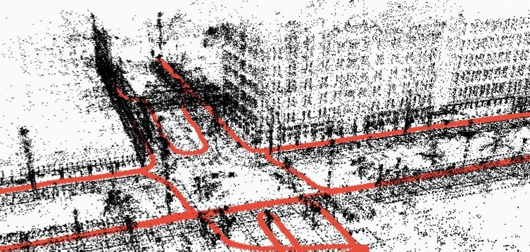
Figure 1: Given a series of 2D images taken by a camera from different positions, the iterative Bundle Adjustment (BA) process evaluates the 3D locations of the objects in the images (in black) and the camera’s poses, as seen in the red trajectory. We propose a method to accelerate the process by reducing the number iterations required for the solving.

SLAM is commonly solved using the iterative Bundle Adjustment (BA) process [9, 21]. In fact, BA occupies roughly $60\%$–$80\%$ of the execution time needed for the mapping [25]. On each iteration the 3D locations and camera poses are first evaluated by a combination of two optimization methods: Gradient descend (GD) and Gauss-Newton (GN), which are weighted according to a damping factor, termed $\lambda$. Then, the evaluated locations are projected into 2D according to the evaluated poses. The stopping criterion (convergence) of this iterative process is usually met when the difference between the evaluated 2D projections and the initially extracted 2D matches (termed projection error) is lower than a certain threshold. Due to computational constraints, if convergence is not achieved within a fixed number of iterations, the process is stopped.

Two main factors influence the execution time: (1) the duration of a single iteration, which is mainly affected by the Hessian’s calculation that GN entails; (2) the required number of iterations to reach convergence, caused by inefficient choosing of $\lambda$. Some previous BA acceleration methods focus on the first factor and reduce the duration of each iteration, by suggesting efficient ways to calculate and invert the sparse Hessian [32, 13]. The focus of this paper is on the second factor—decreasing the number of iterations.

In the classic approach, the value of $\lambda$ is determined heuristically by the Levenberg-Marquardt (LM) algorithm [21] on each iteration. It may change only by one of two specific constant factors between consecutive iterations. This limits the ability to efficiently change the optimization scheme between GD and GN, even when it can be beneficial. We propose to address this problem differently.

Our key idea is to learn a dynamic value of $\lambda$. As the choice of $\lambda$’s value on each iteration may influence the solving for several iterations, we propose to view the process in a new light. Differently from previous approaches, we view the BA process in a holistic manner as a game. We show how a simple Reinforcement Learning (RL) framework suffices to achieve a solution that upholds a dynamic and efficient weighting of GD and GN, which is determined by $\lambda$. Briefly, RL tasks are defined by an environment and an agent. The agent learns to preform actions according to the environment’s response to these actions (at the form of rewards). The agent aims to maximize the sum of the expected rewards, which is the key to handling delayed and sparse rewards like the BA’s single and delayed convergence. In our case, the environment solves the BA problem and its step performs a single BA iteration. As we aim at a learned $\lambda$, we chose to represent the value of $\lambda$ as the agent’s action. The reward is positive only on the iteration convergence is achieved and is negative otherwise. Therefore, in every iteration convergence is not achieved the agent gets a negative reward as a ”fine”. Since the agent aims at maximizing the sum of the expected rewards, it is encouraged to find a valid solution (reach convergence) within as few iterations as possible.

Our method is shown to reduce the number of iterations required to achieve the BA convergence by a factor of $3$-$5$ on both KITTI [10] and BAL [1] benchmarks. Furthermore, our approach is likely to impact common real-life BA problems, whose solving may require much time due to their large size. In addition, we demonstrate that our agent could be trained in a time-efficient manner on small synthetic scenes of randomly chosen locations and camera’s poses, and still accelerate the solving of real-life scenarios. Finally, our approach may be integrated and added to previous works that focus on reducing the time of each iteration [32, 13], but might be less beneficial to other methods such as [23] that suggest hardware-based BA optimizations.

Hence our work makes the following contributions:

1. We propose a general and unified approach that learns the ideal value of $\lambda$. It can be integrated within other BA acceleration methods.

2. We propose a network that utilizes this approach using Reinforcement Learning. We show that it achieves a significant reduction in the number of iterations and running time. On the KITTI benchmark for instance, a $1/5$ of the iterations were required, which led to an overall speedup of $~{}3$.

2 Related Work

Bundle Adjustment (BA). This is a known method to address Simultaneous Localization And Mapping (SLAM) [1, 22, 27, 31, 32] problems. Given a set of 2D key-points (matches), BA [9, 21] aims to solve a system of non-linear equations to evaluate the 3D locations and camera poses according to those matches. Due to the non-linear nature of the equations BA is solved iteratively. On each iteration a Reduced Camera System [14, 19] is solved by two optimization methods that are weighted by a damping factor, $\lambda$. $\lambda$’s value is determined by the Levenberg-Marquardt (LM) [21] algorithm’s heuristic on each iteration as follows: $\lambda$ is multiplied by $1/2$ if the current iteration’s estimation error is larger than that of the previous iteration, or by $2$ otherwise.

Bundle Adjustment Acceleration. As BA is a fundamental problem in various fields and a main efficiency bottleneck for many real-time applications, several works that accelerate it were introduced  [13, 23, 25, 32, 6, 5]. Each work faces the acceleration challenge differently. Tanaka et al. [25] try to replace the BA process entirely by splitting the solving into smaller (”local”) parts, and solve each local part using a Neural Network (NN). ang and Tan [26] also use a NN to solve BA, and learn $\lambda$’s value for a constant number of iterations ($5$). Von Stumberg et al. [29] introduce a Gauss-Newton loss to learn SLAM solving. Oritz et al. [23] replace LM with Gaussian Belief Propagation (GBP) which requires a separate damping factor for each key-point, and use Intelligence Processing Unit (IPU) hardware to improve parallelism capabilities. In [6, 5] Demmel et al. utilize fixed point approximations to accelerate the solving. Other methods focus on accelerating the time of a single iteration. Both Clark et al. [4] and Zhou et al. [32] use a NN to calculate the Jacobian matrix. For instance,  [32] split the BA into smaller problems via clustering. Huang et al. [13] use domain decomposition to split the solving into smaller clusters.  [2, 11] may also be used to optimize BA’s performance. Unlike past works, we focus on reducing the sheer number of iterations of the LM based BA solving. Our iteration reduction could therefore benefit several previous approaches and be added to them.

Reinforcement Learning (RL). This is a growing field of research in machine leaning that has been used for many applications [18, 24, 28, 17, 20, 15, 22]. RL problems are commonly represented by an agent and an environment. Each time the agent preforms an action ($a$), the environment responds by preforming a step according to that action and returns an observation (state $s$) and a reward ($r$). RL problems are defined by their actions, states and rewards that can be either discrete or continuous and of any dimension. The agent chooses its actions according to a stochastic policy $\pi$, which determines the probability to choose each action in the action space. The state provides information about the environment, like the estimation error in our case, while the reward encourages the agent to reach convergence. Value functions ($v$) evaluate the sum of expected future rewards, and are evaluated according to a specific policy, i.e. $v_{\pi}$.

RL is used in various fields including games [24], robotics [16], Natural Language Processing (NLP) [28] and Computer Vision (CV) [17]. It is also used for hyper-parameter tuning of both classic [20] and Deep Leaning (DL) [15] optimization methods. This work is among the first to utilize Deep Reinforcement Learning to choose $\lambda$’s value to accelerate the BA’s optimization problem solving.

Soft Actor Critic (SAC). This is a RL framework that aims at augmenting the standard RL maximum reward objective with an entropy maximization term, which leads to a substantial improvement in exploration [12, 3]. In their work, Haarnoja et al. [12] show that SAC achieves fast and stable convergence on various RL tasks. We chose SAC as our RL framework as it is stable and suites continuous state and action spaces, like in our BA problem. Furthermore, the large number of parameters that need to be updated and estimated on each BA iteration results in many possible solutions. Such a large and complex problem could greatly benefit from SAC’s extensive and sophisticated exploration.

3 Method

Given a series of 2D images taken by a single camera, the Bundle Adjustment (BA) iterative optimization process aims at evaluating the camera’s poses and objects’ 3D locations. Two optimization methods are used for the evaluation on each iteration: Gradient Descend (GD) and Gauss-Newton (GN), that are weighted by a damping factor, $\lambda$.

Although both GD and GN advance in the direction of the gradient, they differ in nature. Generally speaking, the GN takes a bigger step than the GD and is well suited to explore parabolic functions. But, if the local function is not parabolic in nature, the big GN step might divert the solution away from the true minima. In such cases the GD is more effective. But relying on the small GD step alone could lead to a slow and inefficient solving. Therefore, efficient BA solving requires efficient weighing between GD and GN, which is determined by $\lambda$. Recall that in the classic approach, $\lambda$’s value is set by the Levenberg-Marquardt (LM) algorithm and may change by one of two constant factors between consecutive iterations. This may result in inefficient weighting of GD and GN and consequently in a large number of iterations until convergence is achieved.

Our key idea is therefore to learn a dynamic value of $\lambda$, to dynamically weight the two optimization methods in an efficient manner. This is not straight-forward as the BA’s convergence (or failure) is achieved only once at the very end of the solving process, and since each choice of $\lambda$ may affect the solving for several iterations. Therefore, as we aim to reduce the total number of iterations required to reach convergence, the learning of the ideal value of $\lambda$ requires viewing the solving process as a whole.

Hence, differently from previous methods, we propose to view the BA solving process in a new and holistic manner as a game. We may draw an analogy to a chess game, where victory (convergence) is achieved only once at the very end of the game, while each turn (iteration) may go better or worse (estimation error) and the choosing of $\lambda$’s value is analogous to choosing a chess piece and moving it.

Fortunately, Reinforcement Learning (RL) methods are designed to handle continuous processes, such as the BA’s convergence, while producing long-term decisions. This is done by viewing each process in holistic manner, that enables handling sparse and delayed rewards. Hence, RL could be harnessed to learn the optimal value of $\lambda$. Thus, we formulate the BA problem in RL terms by defining states, actions and rewards. As our method is not limited by two constant factors between iterations, it enables a dynamic and efficient weighting of GD and GN along the solving. This may reduce the number of iterations required for convergence and result in a more time-efficient solving process.

We use the Soft Actor Critic (SAC) RL framework, as it is stable and adjusted to continuous state and action spaces like our problem entails, and for its extensive exploration which is beneficial in our highly complex and multi-variable problem [12]. Our method consists of two main parts. The first is an environment which solves a single BA iteration on each step and provides a state and a reward according to it. The second is the SAC agent that predicts the value of $\lambda$ as its action; see Fig. 2. We elaborate on each part hereafter.

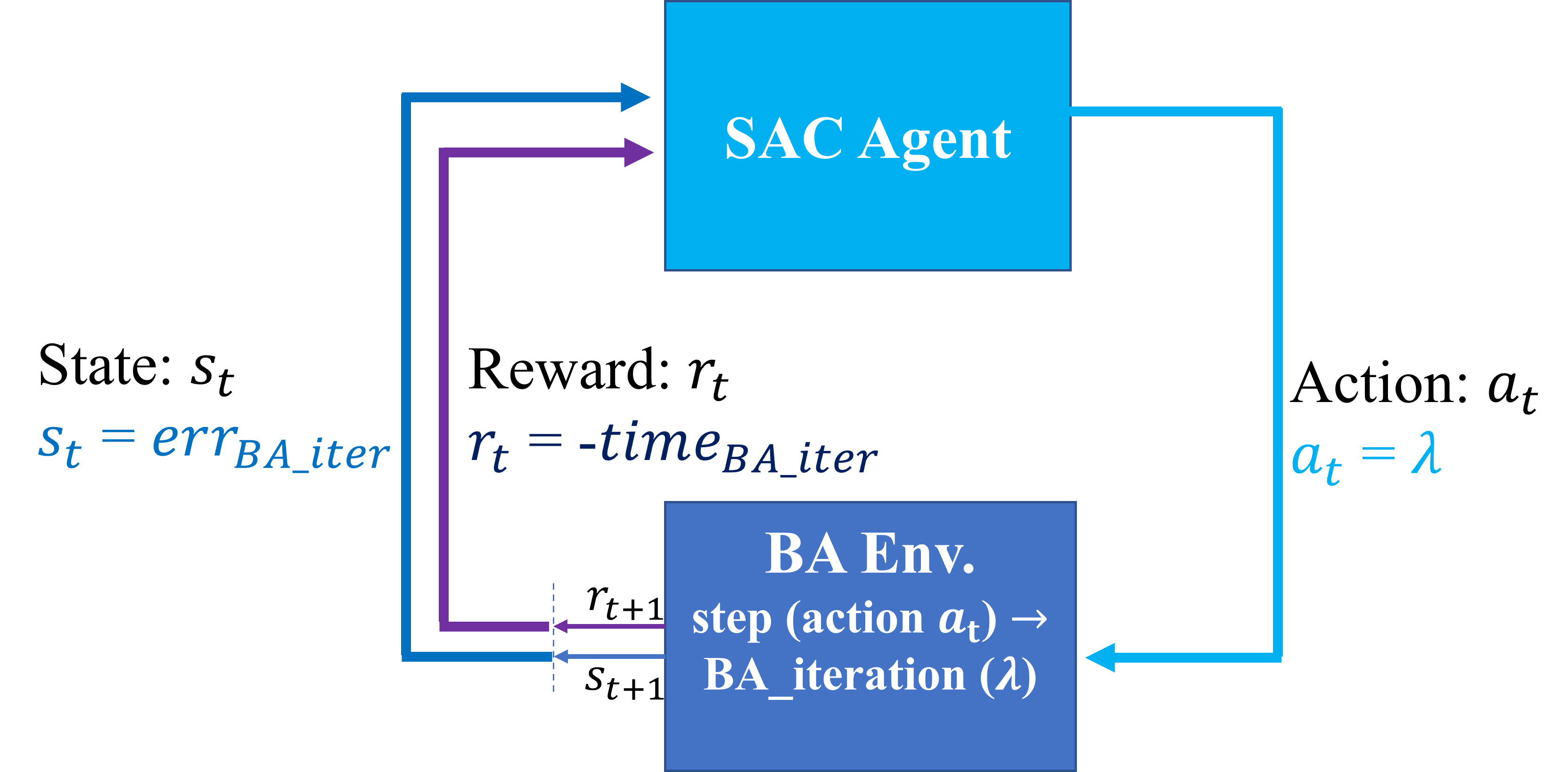
Figure 2: BA problem in RL terms. The SAC agent chooses $\lambda$’s value as its action ($a$), and then the environment preforms a single BA iteration (step), where GD and GN are weighted according to $\lambda$. The environment responds with: 1. a state ($s$) which represents the estimation error of the BA’s iteration; 2. a reward ($r$) that represents the iteration’s duration as a negative (in seconds), except for the iteration convergence is met, where $r$ serves as a positive convergence bonus. As the agent aims at maximizing the sum of expected rewards, it is encouraged to choose $\lambda$ in a manner that reduces the number of solving iterations.

Environment. The environment solves a BA problem. During its initialization, the environment gets a set of 2D matches, representing the projections of the objects’ locations onto the images’ planes, achieved by some key-point based matching process.

On each step (BA iteration), the environment receives $\lambda$ as an action and weighs the GD and GN according to it, as is done in the classic LM scheme. It then estimates the 3D locations of the objects and the camera poses, and projects these locations into 2D according to the estimated poses. The stopping criterion is met when the estimation error is smaller than a certain threshold.

The environment provides an observation (state $s$) and a reward ( $r$) on each iteration (step). Let $z_{ij}$ be the ground truth pixel (match) in which key-point $j$ appeared in image $i$. We model it as a noised projection of 3D-point $q_{j}$ on camera $c_{i}$ with a $w$ Gaussian projection noise, i.e $z_{ij}=Proj(c_{i},q_{j})+w$. Let $\hat{c_{i}},\hat{q_{j}}$ be the current iteration’s estimated poses of the camera $i$ and location of 3D-point $j$ accordingly, and let $\hat{z_{ij}}$ be the respective projection i.e $\hat{z_{ij}}=Proj(\hat{c_{i}},\hat{q_{j}})$. Let $\Delta z_{ij}$ be the difference between the ground truth projection and the estimated projection, i.e. $\Delta z_{ij}=z_{ij}-\hat{z_{ij}}$. Let $C,Q$ be all the estimated camera poses and all the estimated 3D locations respectively. The estimation error is set as the sum of $\Delta z_{ij}$, as follows:

$$\begin{split}&Estimation\,error=\Sigma_{ci}^{C}\Sigma_{qj}^{Q}||{\mathbb{\Sigma}}^{-1/2}\Delta z_{ij}||^{2}\\ &BA_{objective}=argmin_{CQ}[Estimation\,error],\end{split}$$ (1)

where $\mathbb{\Sigma}$ is the covariance matrix, and the state ($s$) is set as a vector of the $5$ last consecutive errors, in order to enable the agent to learn the influence of the choice of $\lambda$ over a few iterations. This forms the connection between the BA solving and the estimation error.

The reward ($r$) is set as the negative of the duration of each iteration (in seconds), apart from the convergence iteration (terminal state) where the reward is set as positive. In standard RL problems the agent is encouraged to maximize the sum of expected rewards:

$$\begin{split}&E_{\pi}=\sum_{t=0}^{\infty}{r_{t}}\\ &r_{t}=-time_{BAiter_{t}}[seconds],\end{split}$$ (2)

where $r_{t}$ is the reward at time step (iteration) $t$ received according to policy $\pi$. In our case, the agent is encouraged to minimize the overall processing time by reaching convergence, which indirectly minimizes the number of iterations.

Soft Actor Critic (SAC). Our SAC framework consists of five networks that are updated according to the known actor-critic iterative optimization scheme:

1. an actor policy network that learns the actions. As we aim at a learned $\lambda$ choosing, we chose the value of $\lambda$ as the one dimensional, real action;

2. two on-policy soft-critic networks, similar in structure, which evaluate the value function and differ in a time-delay;

3. an off-policy value network that evaluates the value function;

4. a target network that converges the values predicted by the on-policy and off-policy networks into a single target value required for the actor-critic optimization.

As the action represents the value of $\lambda$, it influences the optimization process directly. Let $x$ be all the estimated camera’s poses and 3D locations in the BA problem, $J$ be the Jacobin, $H$ be the Hessian, $\Delta z$ be a vector whose entries are $\Delta z_{ij}$ defined before, $\mathbb{\Sigma}$ be the covariance matrix and $\lambda$ be the agent’s action (damping factor). The optimization step taken on each iteration to update $x$ is defined as:

$$\begin{split}&\Delta x=-\frac{1}{\lambda}J(x)^{T}\mathbb{\Sigma}^{-1}\Delta z\\ &{\text{O}ptimization_{gradient}}=-(H+\lambda I)\Delta x.\end{split}$$ (3)

This equation shows $\lambda$’s influence on the Jacobian $J$ and on the Hessian $H$, which impact the GD and GN, respectively.

Following  [7]’s implementation, both soft-critic networks and value network have similar architecture: three FC layers (dim $256$), with Relu as the activation function, as seen in Fig. 3. The value network gets only the state as input, while the two soft-critic networks get both the state and the action. The two differ in a $\tau$ iterations time difference (delay) only, and if one of them reaches a sub-optimal evaluation the other is used instead on each iteration. The target network gets the values (predictions) of the value network and the chosen critic network and predicts a target (value) according to both on each iteration, and has a similar structure to that shown in Fig. 3. The policy network consists of four FC layers (dim $256$) with Relu as the activation function, gets the state as input and predicts the next action. The loss functions of all networks are set to MSE.

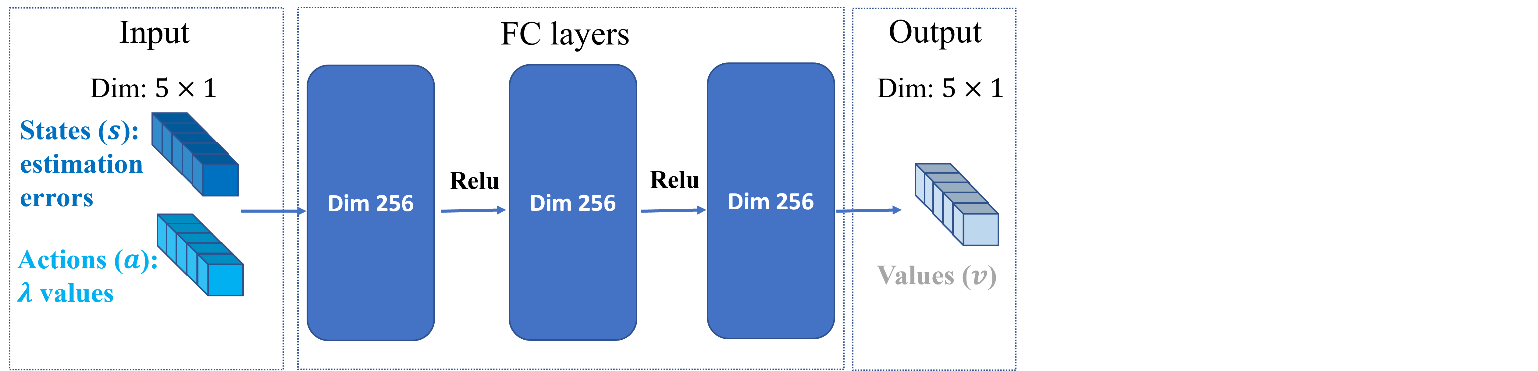
Figure 3: Soft-critic networks and Value network architecture. The networks are similar in structure: $3$ Fully-Connected (FC) layers with Relu as the activation function, following  [7]’s implementation. The value network receives the state vector (dim $5X1$) as input, while both soft-critic networks networks receive the state and the action vectors (dim $5X2$) as input.

4 Experiments

Datasets. We ran our experiments on two real-life large datasets: KITTI [10] and BAL [1], in which each scene may include tens of thousands of points. While BAL provides both the camera poses and the 3D objects’ key-points, KITTI provides only the camera poses with a series of images from which the key-points are extracted.

Results. We compare our results to those of the classic BA approach with LM python implementation [21] and to two recent BA acceleration methods [32, 13]. For each dataset we compare the results to the works that ran on that specific dataset. The stopping condition threshold was set to $1e^{-}6$ for all datasets. As common, if the problem is not solved within $100$ iterations, it is considered as a failure. We use this definition to compare the success rate, but note that all methods achieved $100\%$ success rate on both KITTI [10] and BAL [1]. All time measurements are reported in seconds. Each of the reported times includes both the approach’s set-up time and its BA solving time.

Table 1 compares our results on the KITTI dataset. Our method required $1/5$ of the iterations to succeed in approximately $1/3$ of the time, with the same success rate. Similar results are attained when comparing our results to other approaches on the BAL dataset, as shown in Table 2.

Method	$\#$Iterations	avg. time
[32]	$80$	$287.4$ $[240]$
Ours +  [32]	$16$	$110.0$
Classic	$75$	$340.0$
Ours + classic	$14$	$100.2$

Table 1: Average efficiency improvement - KITTI. Our approach accelerated the solving process by reducing number of iterations of other methods by a factor of $5$. The total time diminished by a factor of $2.5$-$3.2$. The time in the brackets is reported in [32], whereas the time listed is for [32]’s implementation on our hardware.

Method	$\#$Iterations	avg. time
[13]	$15$	$40.75$ $[25.2]$
Ours +  [13]	$5$	$20.3$
Ceres	$20$	$46.7$
Ceres + ours	$4$	$20.75$
Classic	$20$	$110.0$
Ours + classic	$4$	$62.04$

Table 2: Average efficiency improvement - BAL. Our approach accelerated solving process by reducing the number of iterations of other methods by a factor of $3$-$5$. The total time diminished by a factor of $2$. The time in the brackets is reported in [13], whereas the time listed is for [13]’s implementation on our hardware.

We compared the MSE between the final estimations and the ground truth on the BAL [1] dataset, when using [13]’s method with our acceleration. We got similar results (difference $<$ 0.003) to those reported by [13] on the same dataset. This is not surprising as our method accelerates existing approaches and is not supposed to impact their accuracy.

Acceleration based on synthetic data. Both KITTI [10] and BAL [1] contain large scenes, and the scenes sizes directly affect the duration of each BA iteration. Generally speaking, the bigger the scene the longer each iteration is. Hence, utilizing either of these datasets for training requires a considerable amount of time. We created a synthetic random points dataset to simulate smaller scenes, where the duration of each iteration is shorter, which highly reduces the overall training time. This dataset was created by randomly selecting 3D locations (as points) and camera poses. We created $10$ different trajectories, where each trajectory consisted of $10$ camera poses and $10$ locations, which differed between the different trajectories. We used these trajectories to train our agent, which was then tested on KITTI [10] and BAL [1].

Method	Train data	Inference data	$\#$Iterations
Ours +  [32]	Synthetic	KITTI	$16$
Ours + classic	Synthetic	KITTI	$17$
Ours +  [13]	Synthetic	BAL	$5$
Ours + classic	Synthetic	BAL	$5$

Table 3: Average acceleration using synthetic data for training. Our method is able to accelerate the solving of [32, 13] and of the classic approach when trained on synthetic data. The acceleration is similar to that achieved when using KITTI [10] and BAL [1] for training (see Tables 1 and 2), and reduced the number of required iterations by a factor of $3$-$5$.

Table 3 shows that using the synthetic data for training achieves similar acceleration to training on the original datasets. Hence, our solution could be efficiently trained (time wise) on small synthetic scenes, and still successfully accelerate large real-life BA problems.

Comparison to Ceres PCG on BAL. We compare Agarwal et al.’s [1] Ceres PCG C++ implementation to  [13] accelerated by our method over the different BAL dataset’s sub-problems. Table 4 demonstrates that our method leads to a considerable acceleration.

Sub-problem	Ceres-CG	[13]	[13] + ours
Trafalgar	$65.1$	$10.2[1.81]$	$5.6$
Ladybug	$46.7$	$15.35[5.00]$	$8.1$
Dubrovnik	$320$	$10.0[3.14]$	$4.1$
Venice	$1992$	$60[14.2]$	$31.4$
Final	$3897$	$65[24.4]$	$33.7$

Table 4: Acceleration of BAL’s sub-problems. Comparison of the different BAL sub-problems between Agarwal et al.’s [1] Ceres PCG C++ implementation to Huang et al.’s [13] accelerated by our method. All times are reported in seconds. The times in the brackets are reported in [13], whereas the times listed are for  [13]’s run time on our hardware.

Implementation details. Following [7]’s PyTorch implementation, the SAC’s training starts from a series of randomly chosen actions. We used $500$ random choosings. For the classic approach the initial value of $\lambda$ was set to $1/4$. We used a continuous observation space that was set between $-\infty$ and $1000$ and a continuous action space that was set between $0$ and $\infty$. The finish (convergence) bonus reward was set to $10$. The time delay ($\tau$) between the soft-critic networks was set to $5$ iterations. The Adam optimizer was used for all networks. We used a single NVIDIA RTX 3090 GPU for all experiments.

5 Ablation Study

Comparison to a non-holistic learning scheme. Our key idea is to view the BA solving process in a holistic manner and to use RL to learn the ideal value of $\lambda$. We compared our RL approach to a non-holistic learning scheme that tries to learn the value of $\lambda$ by minimizing the estimation error received on each iteration. For fair comparison, we used a network with three FC layers, each at the size of $1280$, so it would have a similar number of parameters to that of the SAC framework. Its input was set as three vectors, representing the last $5$ states, actions and rewards, so it would get the same information as the SAC framework. We term it Zero-net as it aims to minimize the estimation error.

Method	$\#$Iterations
Classic	$20$
Zero-Net + classic	$8$
Ours (holistic) + classic	$\mathbf{4}$

Table 5: Comparison to a non-holistic learning scheme on BAL. Our holistic RL based acceleration method is better than that of the non-holistic Zero-Net method.

We compared Zero-net and our method on the BAL dataset [1]. Our method achieved superior results as seen in Table 5, thus proving the importance of viewing the BA process in a holistic manner.

Method	Batch size	$\#$Iterations
Classic	$-$	$20$
Ours + classic	$1$	$7.5$
Ours + classic	$5$	$\mathbf{4}$
Ours + classic	$10$	$4.5$
Ours + classic	$20$	$5$

Table 6: Acceleration with different state sizes on BAL. The classic approach is accelerated by our method using different state sizes. $5$ achieves the best results.

State size effect. Each state represents $5$ consecutive estimation errors, to enable the agent to learn the influence $\lambda$’s value has over a few iterations. To verify that $5$ iterations are sufficient, we trained our agent on the BAL dataset [1] with different state sizes. The maximal size was set to $20$, as that is the number of iterations the classic approach required for BAL’s solving. Table 6 verifies that $5$ is the optimal state size to enable the learning of $\lambda$’s value.

On the roles of the state and the reward. This work proposes a method to reduce the overall time of the BA process, whilst maintaining the high accuracy that previous methods upheld. We chose to represent the state as the estimation error and to represent the reward as the time. Could these roles be reversed? Could we use the time to represent the state and the estimation error to represent the reward?

Method	$\#$Iterations	Success rate
Classic	$20$	$100\%$
Ours + classic	$\mathbf{4}$	$100\%$
Reversed + classic	$10$	$70\%$

Table 7: Acceleration with opposite state and reward roles. The classic approach is accelerated by our agent and by a ”reversed” agent, which gets each iteration’s duration as a state and the estimation error as a reward. The ”reversed” agent accelerates the solving less than our method and reaches a lower success rate.

We ran such an experiment, attempting to accelerate the solving of the classic approach on the BAL dataset [1], using the duration of each iteration (as a negative) as the state and the estimation error as the reward (with the same finishing bonus). Table 7 compares our acceleration of the classic approach with that of the described ”reversed” environment and agent. The ”reversed” agent accelerated the solving less efficiently than our method, and achieved only $70\%$ success rate which is $30\%$ lower than any other approach. This is probably since the ”reversed” agent aims to minimize the overall error even at the expense of the solving’s duration.

On the choice of the reward. Apart from the convergence iteration (terminal state) where the reward is set as a positive convergence bonus, our reward was set as the duration of each iteration as a negative, which slightly differs between iterations. This raises a question of whether using a constant value as a negative reward ($-1$ in this experiment) instead of the duration would also suffice. Another common reward format in RL is reward reduction, where the reward is set as $0$ in all iterations (states) but convergence (terminal state), and the positive finishing bonus is reduced (by $1\%$ of its value in this experiment) on every iteration. In both cases, the longer it takes the agent to reach convergence, the smaller the sum of its rewards would be. This encourages the agent to reach convergence within as few iterations as possible.

Method	$\#$Iterations
Classic	$20$
Our reward	$\mathbf{4}$
Constant negative reward	$5$
Reward reduction	$4.2$

Table 8: Acceleration with different rewards on BAL. The classic approach is accelerated by our method using different rewards. Using our reward produces better results than using a constant negative value as a reward and from using reward reduction.

Table 8 compares the acceleration results when using all three types of rewards on the BAL dataset [1]. The convergence bonus was set to $10$ in all cases. All reward options successfully accelerated the solving, but our reward achieved the best results, probably due to the extra knowledge about the iterations duration that our reward provides.

Comparison to a constant (non-dynamic) scheduler. As discussed previously, $\lambda$ weights between GD and GN, which impacts the number of iterations required to reach convergence. There seems to be a pattern to the chosen $\lambda$ values. In all the experiments descried in Tables 1 and 2, two small (close to $0$) values of $\lambda$ were chosen, followed by two bigger values.

This raises a question of whether the optimal solution requires a dynamic value of $\lambda$, or would scheduling a series of increasing and decreasing constant values of $\lambda$ suffice to reduce the number of iterations. We tried to use the classic approach with such a scheduler on the BAL dataset [1]. We ran the classic approach accelerated by our method on BAL and extracted a constant series of four $\lambda$ values, that were taken as the average of the test scenes ([$1e-15$, $1e-15$, $0.194$, $0.551$]).

Method	$\#$Iterations	avg. time
Classic	$20$	$110.0$
Constant scheduler	$12$	$80.1$
Classic + ours	$\mathbf{4}$	$\mathbf{62.04}$

Table 9: Comparison to a constant scheduler (non-dynamic method) on BAL. When comparing our method’s acceleration of the classic approach to that of a constant scheduler on the BAL dataset, our dynamic method achieves superior results. The time is reported in seconds.

This four long series was then used repetitively, as a constant (non-dynamic) scheduler to the classic approach. Table 9 shows that our approach needed only a $1/5$ of the iterations required by the classic approach to reach convergence and only a $1/3$ of the iterations required by the constant scheduler. This proves the importance of learning a dynamic value of $\lambda$ which dynamically weights GD and GN. Figure 4 shows an example of one of the described runs, where the value of $\lambda$ changed by a constant factor by the classic approach. On the other hand, our dynamic method enabled $\lambda$’s value remain the same along three consecutive iterations which would not have been possible if a non-dynamic approach was used.

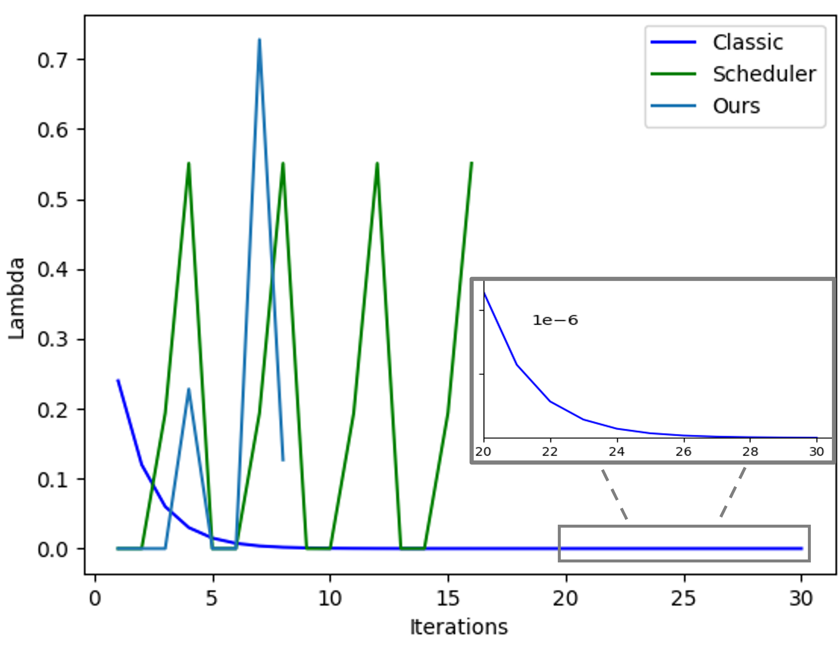
Figure 4: Chosen $\lambda$ values. An example of the chosen $\lambda$ values in a single test case. The classic approach requires $30$ iterations, the scheduler requires $16$ and our approach requires only $8$. We zoom into the last $10$ iterations to demonstrate the decay of $\lambda$’s value to nearly $0$ by the classic approach.

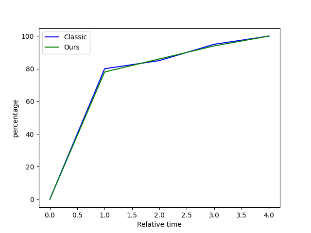
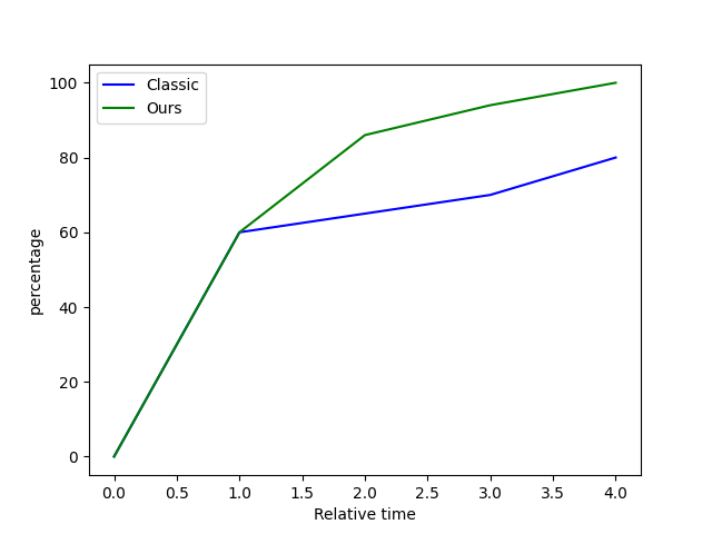
(a) tolerance $\tau=0.1$	(b) tolerance $\tau=0.001$

Figure 5: Performance profile on BAL. (a) When a high tolerance ($\tau=0.1$) is used, the classic solution achieves a full solution very fast and our acceleration is not required. (b) When a more accurate ($\tau=0.001$) solution is required, our method accelerated the solving and reached a more accurate solution.

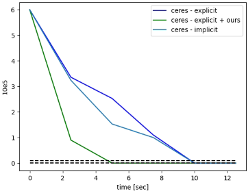
Figure 6: Convergence plot of Ladybug-1197 from BAL. The dashed lines are of tolerances $0.1$ and $0.001$, where explicit stands for PCG and implicit stands for Cholesky’s method.

Convergence plot and performance profile on BAL. Each BA solver requires a different amount of time to solve a given BA problem. Let $\alpha$ be the time required by the fastest solver (e.g. minimal time required) to solve a given BA-problem. Following  [30]’s formulation, performance profiles are used to compare how much of a given BA problem (in percentage) is solved by different solvers, while using $\alpha$ as the relative time. Fig LABEL:fig:tolerence_graphs demonstrates that when a very high threshold ($\tau=0.1$ tolerance) is used, the classic approach reaches a solution within very little time and requires no acceleration. However, when a more accurate solving is required ($\tau=0.001$ tolerance), our acceleration enables reaching higher accuracy within less time.

Convergence plots are used to evaluate the performance of different solvers without using relative time. An example of a convergence plot of scene 1197 from BAL’s Ladybug sub-problem is shown in Fig. 6

Limitations. When considering small BA problems or high tolerance ($\tau=0.1$ threshold for instance), which are commonly solved in a few iterations by the classic approach, we cannot improve them to the same extent as bigger BA problems. For instance, when $5$ random points and $5$ random camera poses are used, the classic approach reaches convergence within $5$ iterations on average while our method required $4$ iterations on average. Furthermore, our method’s overall solving time was $1/2$ a second longer than that of the classic approach in this case, due to the agent’s inference time. Therefore, when considering small or inaccurate solving of BA problems our method is less effective, and may even perform worse on extremely small problems.

6 Conclusion

Localization and mapping are key problems in many real time applications, that are commonly solved using the iterative Bundle Adjustment (BA) process. On each BA iteration, a system of non-linear equations is solved using two optimization methods: Gradient Descend (GD) and Gauss-Newton (GN), each better suited for different parts of the solving. In the classic approach, these two methods are weighted by a damping factor, $\lambda$, that may change by one of two constant factors between consecutive iterations. This may prevent the classic approach from efficiently weighting between GD and GN which might result in many iterations.

Our key idea is therefore to learn a dynamic value of $\lambda$ in order to reduce the sheer number of iterations required to reach convergence by efficiently weighting GD and GN. This is not trivial as the solving needs to be considered as a whole in order to learn from it. Hence, differently from past approaches, we propose to view the BA process in a holistic manner as a game. We use a Reinforcement Learning (RL) based method to learn $\lambda$, as it can handle sparse and delayed rewards like the BA’s convergence and views the BA process as a whole. We use the Soft Actor Critic (SAC) RL framework as it is stable, well suited for continuous state and action spaces, and for its extensive exploration.

We set an environment that solves the non-linear equations system, and an agent who’s action determines the value of $\lambda$. The reward is set as negative in all iterations, apart from the convergence iteration where the reward serves as a positive convergence bonus. As the agent aims at maximizing the sum of expected rewards, it is encouraged to solve the problem within as few iterations as possible. This is the key to our method’s time reduction.

Our RL based solving approach is shown to reduce the number of iterations required to reach convergence by a factor of $3-5$ on both known KITTI [10] and BAL [1] benchmarks. Our reduction could be especially meaningful in real life scenarios that may require much time to solve due to their large size. Our agent may also be trained on small synthetic scenes, which is highly time-efficient, and still accelerate the solving of bigger real-life scenarios. Moreover, our approach may be added to previous acceleration methods that focus on reducing the time of each iteration, as demonstrated on two different methods. However, hardware based BA optimization methods such as [30, 23, 6] may benefit less from our acceleration.

For future work we would like to further optimize the agent’s architecture to the task at hand, and extend this method to other optimization problems, such as SfM.

Acknowledgements. We gratefully acknowledge the support of the Israel Science Foundation (ISF) 2329/22. We thank Evyatar Bluzer, Maurizio Monge, True Price, Ruibin Ma, Jonathan Zeltser, Omri Carmi and Jan-Michael Frahm for their valuable comments and assistance.

References

- [1] Sameer Agarwal, Noah Snavely, Steven M Seitz, and Richard Szeliski. Bundle adjustment in the large. In European conference on computer vision, pages 29–42. Springer, 2010.
- [2] Brandon Amos and J. Zico Kolter. Optnet: Differentiable optimization as a layer in neural networks. CoRR, abs/1703.00443, 2017.
- [3] Petros Christodoulou. Soft actor-critic for discrete action settings. arXiv preprint arXiv:1910.07207, 2019.
- [4] Ronald Clark, Michael Bloesch, Jan Czarnowski, Stefan Leutenegger, and Andrew J. Davison. Ls-net: Learning to solve nonlinear least squares for monocular stereo. CoRR, abs/1809.02966, 2018.
- [5] Nikolaus Demmel, David Schubert, Christiane Sommer, Daniel Cremers, and Vladyslav Usenko. Square root marginalization for sliding-window bundle adjustment. In Proceedings of the IEEE/CVF International Conference on Computer Vision (ICCV), pages 13260–13268, October 2021.
- [6] Nikolaus Demmel, Christiane Sommer, Daniel Cremers, and Vladyslav Usenko. Square root bundle adjustment for large-scale reconstruction. In Proceedings of the IEEE/CVF Conference on Computer Vision and Pattern Recognition (CVPR), pages 11723–11732, June 2021.
- [7] Zihan Ding. Popular-rl-algorithms. https://github.com/quantumiracle/Popular-RL-Algorithms, 2019.
- [8] Meiling Fang, Thomas Pollok, and Chengchao Qu. Merge-sfm: Merging partial reconstructions. In BMVC, page 29, 2019.
- [9] F Dan Foresee and Martin T Hagan. Gauss-newton approximation to bayesian learning. In Proceedings of international conference on neural networks (ICNN’97), volume 3, pages 1930–1935. IEEE, 1997.
- [10] Andreas Geiger, Philip Lenz, Christoph Stiller, and Raquel Urtasun. Vision meets robotics: The kitti dataset. The International Journal of Robotics Research, 32(11):1231–1237, 2013.
- [11] Edward Grefenstette, Brandon Amos, Denis Yarats, Phu Mon Htut, Artem Molchanov, Franziska Meier, Douwe Kiela, Kyunghyun Cho, and Soumith Chintala. Generalized inner loop meta-learning. CoRR, abs/1910.01727, 2019.
- [12] Tuomas Haarnoja, Aurick Zhou, Kristian Hartikainen, George Tucker, Sehoon Ha, Jie Tan, Vikash Kumar, Henry Zhu, Abhishek Gupta, Pieter Abbeel, et al. Soft actor-critic algorithms and applications. arXiv preprint arXiv:1812.05905, 2018.
- [13] Jingwei Huang, Shan Huang, and Mingwei Sun. Deeplm: Large-scale nonlinear least squares on deep learning frameworks using stochastic domain decomposition. In Proceedings of the IEEE/CVF Conference on Computer Vision and Pattern Recognition, pages 10308–10317, 2021.
- [14] Yekeun Jeong, David Nister, Drew Steedly, Richard Szeliski, and In-So Kweon. Pushing the envelope of modern methods for bundle adjustment. IEEE transactions on pattern analysis and machine intelligence, 34(8):1605–1617, 2011.
- [15] Hadi S. Jomaa, Josif Grabocka, and Lars Schmidt-Thieme. Hyp-rl : Hyperparameter optimization by reinforcement learning. CoRR, abs/1906.11527, 2019.
- [16] Jens Kober, J Andrew Bagnell, and Jan Peters. Reinforcement learning in robotics: A survey. The International Journal of Robotics Research, 32(11):1238–1274, 2013.
- [17] Ngan Le, Vidhiwar Singh Rathour, Kashu Yamazaki, Khoa Luu, and Marios Savvides. Deep reinforcement learning in computer vision: A comprehensive survey. CoRR, abs/2108.11510, 2021.
- [18] Yuxi Li. Deep reinforcement learning: An overview. arXiv preprint arXiv:1701.07274, 2017.
- [19] Manolis IA Lourakis and Antonis A Argyros. Sba: A software package for generic sparse bundle adjustment. ACM Transactions on Mathematical Software (TOMS), 36(1):1–30, 2009.
- [20] Nina Mazyavkina, Sergey Sviridov, Sergei Ivanov, and Evgeny Burnaev. Reinforcement learning for combinatorial optimization: A survey. Computers & Operations Research, 134:105400, 2021.
- [21] Jorge J Moré. The levenberg-marquardt algorithm: implementation and theory. In Numerical analysis, pages 105–116. Springer, 1978.
- [22] Kai Ni, Drew Steedly, and Frank Dellaert. Out-of-core bundle adjustment for large-scale 3d reconstruction. In 2007 IEEE 11th International Conference on Computer Vision, pages 1–8. IEEE, 2007.
- [23] Joseph Ortiz, Mark Pupilli, Stefan Leutenegger, and Andrew J Davison. Bundle adjustment on a graph processor. In Proceedings of the IEEE/CVF Conference on Computer Vision and Pattern Recognition, pages 2416–2425, 2020.
- [24] Richard S Sutton and Andrew G Barto. Reinforcement learning: An introduction. MIT press, 2018.
- [25] Tetsuya Tanaka, Yukihiro Sasagawa, and Takayuki Okatani. Learning to bundle-adjust: A graph network approach to faster optimization of bundle adjustment for vehicular slam. In Proceedings of the IEEE/CVF International Conference on Computer Vision, pages 6250–6259, 2021.
- [26] Chengzhou Tang and Ping Tan. BA-net: Dense bundle adjustment networks. In International Conference on Learning Representations, 2019.
- [27] Bill Triggs, Philip F McLauchlan, Richard I Hartley, and Andrew W Fitzgibbon. Bundle adjustment—a modern synthesis. In International workshop on vision algorithms, pages 298–372. Springer, 1999.
- [28] Víctor Uc-Cetina, Nicolás Navarro-Guerrero, Anabel Martín-González, Cornelius Weber, and Stefan Wermter. Survey on reinforcement learning for language processing. CoRR, abs/2104.05565, 2021.
- [29] Lukas von Stumberg, Patrick Wenzel, Qadeer Khan, and Daniel Cremers. Gn-net: The gauss-newton loss for deep direct SLAM. CoRR, abs/1904.11932, 2019.
- [30] Simon Weber, Nikolaus Demmel, Tin Chon Chan, and Daniel Cremers. Power bundle adjustment for large-scale 3d reconstruction, 2023.
- [31] Changchang Wu, Sameer Agarwal, Brian Curless, and Steven M Seitz. Multicore bundle adjustment. In CVPR 2011, pages 3057–3064. IEEE, 2011.
- [32] Lei Zhou, Zixin Luo, Mingmin Zhen, Tianwei Shen, Shiwei Li, Zhuofei Huang, Tian Fang, and Long Quan. Stochastic bundle adjustment for efficient and scalable 3d reconstruction. In European Conference on Computer Vision, pages 364–379, 2020.
- [33] Siyu Zhu, Tianwei Shen, Lei Zhou, Runze Zhang, Jinglu Wang, Tian Fang, and Long Quan. Parallel structure from motion from local increment to global averaging. arXiv preprint arXiv:1702.08601, 2017.
- [34] Siyu Zhu, Runze Zhang, Lei Zhou, Tianwei Shen, Tian Fang, Ping Tan, and Long Quan. Very large-scale global sfm by distributed motion averaging. In Proceedings of the IEEE conference on computer vision and pattern recognition, pages 4568–4577, 2018.